Abstract

The precise knowledge of the QED initial state corrections is of instrumental importance in studying high luminosity measurements in $e^{+}e^{-}$ annihilation at facilities like LEP, the International Linear Collider ILC, CLIC, a Giga-$Z$ facility, and the planned FCC_ee. Logarithmic corrections of up to $O(\alpha^{6}L^{5})$ are necessary with various subleading terms taken into account. This applies to both the inclusive measurement of processes like $e^{+}e^{-}\rightarrow\gamma^{*}/Z^{*}$ and also the forward–backward asymmetry. As has been shown recently, techniques from massive QCD, such as the computation of massive on–shell operator matrix elements, can be used for these calculations. We give an introduction to this topic and present both the calculation methods and the numerical corrections having been reached so far.

1 Introduction

The precision physics for the process $e^{+}e^{-}\rightarrow\gamma^{*}/Z^{*}$ started at LEP-1 in the early 1990ies leading to a highly precise measurement of the $Z$–peak [1]. Among other radiative corrections the QED initial state corrections are of high importance in these measurements, since they change the shape–parameters of the $Z$–peak significantly. The most far–reaching calculation of the initial state QED corrections (ISR) of $O(\alpha^{2})$, with $\alpha=4\pi a$ the fine structure constant, had been performed in Ref. [2] at that time, which had been a theoretical challenge and milestone. This calculation has never been checked until 2011, some time after LEP had already been ended, when the same result was derived using massive operator matrix elements (OMEs) in Ref. [3]. Massive operator elements were known to present all contributions except power corrections in QCD in the cases with external massless partons [4]. Therefore, one could try to apply this method also in the case of massive fermions, the electrons. However, the present case is one with also massive external lines. After correcting typographical errors in [2] all logarithmic contributions of both calculations [2, 3] and the constant term at $O(\alpha)$ agreed, but not the result for the constant term of $O(\alpha^{2})$. Furthermore, in one of the subprocesses Ref. [2] agreed with [5]. Due to this, one option to explain the observed differences has been that the method of massive OMEs does not work in the case of massive external lines, or, otherwise, that the results in Refs. [2, 5] need corrections.

One way to unambiguously resolve these discrepancies has been to repeat the complete calculation to $O(\alpha^{2})$ without neglecting any term at intermediate steps and carry out the limit $m_{e}^{2}/s\rightarrow 0$ for the power corrections only in the final results. Such a calculation has not been fully possible in 2011, but became accessible in 2019, again working on complete QCD calculation in which specific phase space integrals occurred. The organization of these integrals as iterated integrals over various root–valued letters, cf. e.g. [6, 7], and their reduction using shuffle algebras [8], brought the solution to also organize the phase–space integrals in the case of QED. In this way, we firstly found the correct results for the fermionic non–singlet corrections of [2, 5], if the radiated particles are electrons, but not muons, [9]. While our result agreed with [2, 5] for muons, it disagreed for electron radiation, since there electron mass terms had been neglected too early in Refs. [2, 5]. For Ref. [2] this also applied to the pure singlet channel, which has been calculated earlier in the massless case in QCD in Ref. [10], and been used as such in [2]. However, also here electron mass terms cannot be neglected. We also newly calculated the bosonic contributions in [11, 12], and fully confirmed the results given in Ref. [3] by the phase space integration method intended to be used in Ref. [2]. Through this we proofed that the method of massive OMEs can also be used in the case of external massive fermionic lines.

The technique of massive OMEs now also allows to access logarithmically enhanced terms through the renormalization group. With the known pieces it is possible to obtain three consecutive logarithmic orders in all higher orders in $\alpha$, as e.g. $O(\alpha^{3}L^{3}),O(\alpha^{3}L^{2}),O(\alpha^{3}L)$, etc., with $L=\ln(s/m_{e}^{2})$ and $s$ the $cms$ energy. We applied this technique to all corrections up to $O(\alpha^{6}L^{5})$ in Ref. [13] and to higher order corrections to the forward–backward asymmetry [14], although in this case new contributions have to be calculated. We also note that the universal QED corrections $O(\alpha^{k}L^{k})$ are known to at least fifth order $k=5$, cf. [15, 16, 17, 18, 19, 20, 21, 22]. Highly precise QED radiative corrections are of importance for the analysis of the precision measurements at LEP, [1], the planned international linear collider, ILC, [23, 24, 25] CLIC [26], the FCC_ee [27] and muon colliders [28].

The paper is organized as follows. In Section 2 we describe the direct calculation of the $O(\alpha^{2})$ corrections due to initial state radiation and the factorized approach by using massive OMEs, which lead to the same results. For the $O(\alpha^{2})$ ISR corrections we present numerical results on the $Z^{0}$-peak and width, for the process $e^{+}e^{-}\rightarrow Z^{0}H$ and $t\bar{t}$ production in the threshold region. The method of massive OMEs is then extended to higher orders for the leading and two subleading logarithmic terms in Section 3. In Section 4 we present precision results for the forward–backward asymmetry and Section 5 contains the conclusions. We also present numerical results on the calculated radiative corrections for different key observables.

2 Two–loop Corrections

After observing the differences in the results of Refs. [3] and [2], the only way to clarify this consisted in a direct calculation of the complete $O(a^{2})$ initial state corrections to $e^{+}e^{-}\rightarrow\gamma^{*}/Z^{*}$ annihilation. Its result confirmed the results of Ref. [3]. Due to this the explicit high energy factorization could be shown to $O(a^{2})$ also for massive external fermions. Assuming this factorization to even higher orders, allows to calculate the first three logarithmic correction terms to even higher order. These results are reported in Section 3. In the following we first summarize the complete $O(a^{2})$ calculation in Section 2.1 and turn then to the calculation based on massive OMEs in Section 2.2. Finally, we derive numerical results on the $O(a^{2})$ corrections for a series of key processes to be measured at future facilities.

2.1 Two–loop Corrections: the Direct Calculation

Upon neglecting power corrections of $O(m_{e}^{2}/s)$ the initial state QED corrections can be written in terms of the following functions

$$H\left(z,\alpha,\frac{s}{m^{2}}\right) = \delta(1-z)+\sum_{k=1}^{\infty}\left(\frac{\alpha}{4\pi}\right)^{k}C_{k}\left(z,\frac{s}{m^{2}}\right)$$ (1)

$$C_{k}\left(z,\frac{s}{m^{2}}\right) = \sum_{l=0}^{k}\ln^{k-l}\left(\frac{s}{m^{2}}\right)c_{k,l}(z),$$ (2)

which yield the respective differential cross sections by

$$\frac{d\sigma_{e^{+}e^{-}}}{ds^{\prime}}=\frac{1}{s}\sigma_{e^{+}e^{-}}(s^{\prime})H\left(z,\alpha,\frac{s}{m^{2}}\right),$$ (3)

with $\sigma_{e^{+}e^{-}}(s^{\prime})$ the scattering cross section without the ISR corrections, $\alpha\equiv\alpha(s)$ the fine structure constant and $z=s^{\prime}/s$, where $s^{\prime}$ is the invariant mass of the produced (off-shell) $\gamma/Z$ boson.

The Born cross section is given by

$$\sigma^{(0)}_{e^{+}e^{-}}(s) = \frac{4\pi\alpha^{2}}{3s}N_{C,f}\sqrt{1-\frac{4m_{f}}{s}}\left[\left(1+\frac{2m_{f}^{2}}{s}\right)G_{1}(s)-6\frac{m_{f}^{2}}{s}G_{2}(s)\right],$$ (4)

see e.g. [29], where $N_{C,f}$ denotes the color factor for the final state fermions, i.e. $N_{C}=3$ for quarks and $N_{C}=1$ for leptons. The effective couplings $G_{i}(s)|_{i=1...2}$ read

$$G_{1}(s) = Q_{e}^{2}Q_{f}^{2}+2Q_{e}Q_{f}v_{e}v_{f}{\sf Re}[\chi_{Z}(s)]+(v_{e}^{2}+a_{e}^{2})(v_{f}^{2}+a_{f}^{2})|\chi_{Z}(s)|^{2},$$ (5)

$$G_{2}(s) = (v_{e}^{2}+a_{e}^{2})a_{f}^{2}|\chi_{Z}(s)|^{2},$$ (6)

where the reduced $Z$–propagator is given by

$$\chi_{Z}(s)=\frac{s}{s-M_{Z}^{2}+iM_{Z}\Gamma_{Z}},$$ (7)

with $M_{Z}$ and $\Gamma_{Z}$ the mass and the with of the $Z$–boson and $m_{f}$ is the mass of the final state fermion. $Q_{e,f}$ are the electromagnetic charges of the electron $(Q_{e}=-1)$ and the final state fermion, respectively, and the electro–weak couplings $v_{i}$ and $a_{i}$ are given by

$$v_{e} = \frac{1}{\sin\theta_{w}\cos\theta_{w}}\left[I^{3}_{w,e}-2Q_{e}\sin^{2}\theta_{w}\right],$$ (8)

$$a_{e} = \frac{1}{\sin\theta_{w}\cos\theta_{w}}I^{3}_{w,e},$$ (9)

$$v_{f} = \frac{1}{\sin\theta_{w}\cos\theta_{w}}\left[I^{3}_{w,f}-2Q_{f}\sin^{2}\theta_{w}\right],$$ (10)

$$a_{f} = \frac{1}{\sin\theta_{w}\cos\theta_{w}}I^{3}_{w,f}\leavevmode\nobreak\ ,$$ (11)

where $\theta_{w}$ is the weak mixing angle, and $I^{3}_{w,i}=\pm 1/2$ the third component of the weak isospin for up and down particles, respectively.

One may distinguish four processes: i) photon radiation, ii) $e^{+}e^{-}$ pair emission, iii) fermionic pure singlet corrections, and iv) the interference terms between the diagrams contributing to ii) and iii). Furthermore, there is also $\mu^{+}\mu^{-}$ initial state radiation and that of light quarks. The latter contribution belongs to the QCD corrections, and we will label the one of $\mu^{+}\mu^{-}$ pair emission as process v). It has been described in Refs. [2, 5] correctly, as has been confirmed in Ref. [9, 11]. We will consider the processes i)–iv) in the following.

The phase–space integrals to be performed are organized as iterated integrals over a set of letters, which are found by solving associated differential equations, cf. [30]. The alphabet consists of letters forming generalized harmonic polylogarithms [31], but also of elliptic letters. Since all integrations are indefinite, still iterative integrals are obtained. We therefore call the corresponding integrals Kummer–elliptic integrals. The respective iterative integrals have the structure

$$H_{b,\vec{a}}(z)=\int_{0}^{z}dyf_{b}(y)H_{\vec{a}}(y).$$ (12)

Examples for these letters are, cf. [11] (using the abbreviation $f_{b}(t;z,\rho)\equiv f_{b}$),

$$d_{24} = \frac{1}{\big{(}t^{2}(1-z)^{2}-8\rho(1+z)t+4tz+16\rho^{2}\big{)}\sqrt{t^{2}(1-z)^{2}-8\rho t(1+z)+16\rho^{2}}},$$ (13)

$$d_{26} = \frac{1}{\sqrt{1-t}\big{(}t^{2}(1-z)^{2}-8\rho(1+z)t+4tz+16\rho^{2}\big{)}\sqrt{t^{2}(1-z)^{2}-8\rho t(1+z)+16\rho^{2}}}.$$ (14)

These integrals depend on the tiny parameter $\rho=m_{e}^{2}/s$ and one may now expand in $\rho$ controlling the accuracy by high precision numerics for the unexpanded integrals at each step. One finally arrives at iterated integrals which integrate in terms of harmonic polylogarithms or even classical polylogarithms and Nielsen integrals [32, 33, 34, 35, 36, 37].

The size of the amplitudes to be dealt with amounts to 10 Gb (process i)), 25 kb (process ii)), 56 kb (process iii)) and 124 kb (process iv)), requiring several months for code design and 30h of computation time. The calculation could only be done by using computer–algorithmic methods, which have been developed very recently.

The 2–loop corrections for process i) consist out of soft (S), virtual (V) and hard (H) corrections and their interference terms [11] which can be written schematically by

$$R^{\gamma\gamma}_{2}=T_{2}^{\rm S_{2}}+T_{2}^{\rm V_{2}}+T_{2}^{\rm S_{1}V_{1}}+T_{2}^{\rm S_{1}H_{1}}+T_{2}^{\rm V_{1}H_{1}}+T_{2}^{\rm H_{2}}.$$ (15)

We agree with [2] for all but the virtual–hard contributions, i.e. $T_{2}^{\rm V_{1}H_{1}}$. The radiator $R_{2}^{\gamma\gamma}$ is given by

$$R^{\it i)}_{2}(z) = R_{2}^{\gamma\gamma}(z)$$ (16)

$$= \delta(1-z)\Bigl{\{}32(L-1)^{2}\ln^{2}(\varepsilon)+\big{(}48L^{2}-(112-64\zeta_{2})L+64-64\zeta_{2}\big{)}\ln(\varepsilon)$$

$$+(18-32\zeta_{2})L^{2}-(45-88\zeta_{2}-48\zeta_{3})L+76+(6-96\ln(2))\zeta_{2}-72\zeta_{3}-\frac{96}{5}\zeta_{2}^{2}\Bigr{\}}$$

$$+\theta(1-z-\varepsilon)\Bigl{\{}64(L-1)^{2}{\cal D}_{1}+\big{(}48L^{2}-(112-64\zeta_{2})L+64-64\zeta_{2}\big{)}{\cal D}_{0}$$

$$-L^{2}\biggl{(}8(5+z)+32(1+z)\ln(1-z)+\frac{8\big{(}1+3z^{2}\big{)}}{1-z}\ln(z)\biggr{)}+L\biggl{(}8(14+z)$$

$$+\frac{8\big{(}5+2z+7z^{2}\big{)}}{1-z}\ln(z)-\frac{4\big{(}1+3z^{2}\big{)}}{1-z}\ln^{2}(z)+\frac{16\big{(}1+z^{2}\big{)}}{1-z}\text{Li}_{2}(1-z)$$

$$-32(1+z)\zeta_{2}+\biggl{[}64(1+z)+\frac{16\big{(}1+z^{2}\big{)}}{1-z}\ln(z)\biggr{]}\ln(1-z)\biggr{)}-\frac{8\big{(}18+z-15z^{2}\big{)}}{3(1-z)}$$

$$-\frac{8\big{(}1+z^{2}\big{)}}{3(1-z)}\ln^{3}(z)+\frac{4}{3(1-z)^{3}}\big{(}12-33z+51z^{2}-51z^{3}+13z^{4}\big{)}\ln^{2}(z)$$

$$+\frac{32}{3}(3+8z)\zeta_{2}-32(1+z)\zeta_{3}-\biggl{(}16(1+3z)+\frac{8\big{(}2+6z-3z^{2}\big{)}}{1-z}\ln(z)$$

$$-\frac{8\big{(}3-z^{2}\big{)}}{1-z}\ln^{2}(z)\biggr{)}\ln(1-z)+16z\ln^{2}(1-z)-\biggl{(}\frac{8\big{(}6+3z+26z^{2}-27z^{3}\big{)}}{3(1-z)^{2}}$$

$$+\frac{16\big{(}1-3z^{2}\big{)}}{1-z}\zeta_{2}\biggr{)}\ln(z)+\biggl{(}-\frac{8\big{(}9+19z-13z^{2}\big{)}}{3(1-z)}-16(1+z)\ln(1-z)$$

$$+\frac{8\big{(}5-3z^{2}\big{)}}{1-z}\ln(z)\biggr{)}\text{Li}_{2}(1-z)+24(1+z)\text{Li}_{3}(1-z)+32(1+z)\text{Li}_{3}(z)\Bigr{\}},$$

with

$${\cal D}_{k}(z)=\left(\frac{\ln^{k}(1-z)}{1-z}\right)_{+}.$$ (17)

Here the separation parameter $\varepsilon$ has been introduced to realize the $+$-distributions in terms of functions. It disappears after the $z$-integral has been performed.

Another radiator is the one of the non–singlet process for $e^{+}e^{-}$ emission, $R^{\it ii)}_{2}$. The correction to the scattering cross section for electron pair emission is given by

$$R_{2}^{\it ii)}(z) =\Biggl{\{}\frac{64}{3}z(1-z)(1+z-4\rho){\rm H}^{*}_{v_{4},d_{7}}+\frac{256}{3}z\rho(1+z-4\rho){\rm H}^{*}_{v_{4},d_{6}}$$

$$+\frac{128z(1-4\rho^{2})(1-z+2\rho)(1-z-4\rho)}{3(1-z)^{2}}{\rm H}^{*}_{d_{8},d_{7}}$$

$$+\frac{512z\rho(1-4\rho^{2})(1-z+2\rho)(1-z-4\rho)}{3(1-z)^{3}}{\rm H}^{*}_{d_{8},d_{6}}$$

$$+\frac{16}{9(1-z)^{2}}\Bigl{[}(1+z)^{2}\big{(}4-9z+4z^{2}\big{)}+2\big{(}9-16z+13z^{2}-2z^{3}\big{)}\rho+32\rho^{2}\Bigr{]}{\rm H}^{*}_{d_{2}}$$

$$+\frac{512z\rho}{9(1-z)^{4}}\Bigl{[}3(1-z)^{4}z-(1-z)^{3}\big{(}4+z^{2}\big{)}\rho-2\big{(}9-29z+38z^{2}-17z^{3}+3z^{4}\big{)}\rho^{2}$$

$$-4(2-z)\big{(}3+6z-5z^{2}\big{)}\rho^{3}+16\big{(}7-8z+9z^{2}\big{)}\rho^{4}+128(3-z)\rho^{5}\Bigr{]}{\rm H}^{*}_{d_{4}}$$

$$-\frac{16}{9(1-z)^{4}}\Bigl{[}3-34z+129z^{2}-212z^{3}+129z^{4}-34z^{5}+3z^{6}+8\big{(}2-16z+9z^{2}$$

$$+4z^{3}-5z^{4}+2z^{5}\big{)}\rho+16z\big{(}12-13z+18z^{2}-z^{3}\big{)}\rho^{2}+32\big{(}1+22z-7z^{2}\big{)}\rho^{3}\Bigr{]}{\rm H}^{*}_{d_{1}}$$

$$-\frac{128z}{9(1-z)^{4}}\Bigl{[}1+7z-47z^{2}+86z^{3}-47z^{4}+7z^{5}+z^{6}-2\big{(}7-55z+54z^{2}$$

$$+16z^{3}-17z^{4}+3z^{5}\big{)}\rho-4\big{(}39-16z+16z^{2}+4z^{3}+5z^{4}\big{)}\rho^{2}$$

$$+16\big{(}8-23z+22z^{2}+9z^{3}\big{)}\rho^{3}+128\big{(}7+2z-z^{2}\big{)}\rho^{4}\Bigr{]}{\rm H}^{*}_{d_{5}}-\frac{64}{3}(2z+(1-z)\rho){\rm H}^{*}_{d_{3}}$$

$$+\biggl{[}\frac{16}{3\sqrt{1-4\rho}}(1+z-4\rho){\rm H}^{*}_{v_{4}}+\frac{32(1-4\rho^{2})(1-z+2\rho)(1-z-4\rho)}{3(1-z)^{3}\sqrt{1-4\rho}}{\rm H}^{*}_{d_{8}}\biggr{]}$$

$$\times\ln\left(\frac{1-z-4\rho-\sqrt{1-4\rho}\sqrt{(1-z)^{2}-8(1+z)\rho+16\rho^{2}}}{1-z-4\rho+\sqrt{1-4\rho}\sqrt{(1-z)^{2}-8(1+z)\rho+16\rho^{2}}}\right)\Biggr{\}}.$$ (18)

It can even be obtained without expanding in the parameter $\rho$. Here the iterative integrals ${\rm H}^{*}$ read

$${\rm H}^{*}_{b,\vec{a}}(z)=\int_{z}^{1}dyf_{b}(y){\rm H}^{*}_{\vec{a}}(y)\leavevmode\nobreak\$$ (19)

and the respective letters are given in Ref. [11].

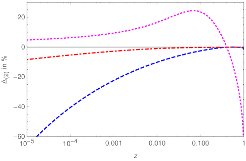
Figure 1: Relative deviations of the results of Ref. [2] from the exact result in % for the $O(\alpha^{2})$ corrections. The non–singlet contribution (process II): dash-dotted line; the pure singlet contribution (process III): dashed; the interference term between both contributions (process IV): dots; for $s=M_{Z}^{2}$, $M_{Z}=91.1879$ GeV; from [9].

After the expansion in $\rho$ one obtains

$$R_{2}^{\it ii)}(z) =\frac{8\big{(}1+z^{2}\big{)}}{3(1-z)}L^{2}+\biggl{[}-\frac{16\big{(}11-12z+11z^{2}\big{)}}{9(1-z)}+\frac{32\big{(}1+z^{2}\big{)}}{3(1-z)}\ln(1-z)$$

$$-\frac{16\big{(}1+z^{2}\big{)}}{3(1-z)}\ln(z)\biggr{]}L+\frac{32\big{(}1+z^{2}\big{)}}{3(1-z)}\ln^{2}(1-z)-\frac{16z^{2}}{3(1-z)}\text{Li}_{2}(1-z)$$

$$+\frac{32}{9(1-z)^{3}}\big{(}7-13z+8z^{2}-13z^{3}+7z^{4}\big{)}-\frac{16z}{9(1-z)^{4}}\big{(}3-36z+94z^{2}$$

$$-72z^{3}+19z^{4}\big{)}\ln(z)-\frac{32\big{(}1+z^{2}\big{)}}{3(1-z)}\zeta_{2}-\biggl{(}\frac{32\big{(}11-12z+11z^{2}\big{)}}{9(1-z)}$$

$$+\frac{32\big{(}1+z^{2}\big{)}}{3(1-z)}\ln(z)\biggr{)}\ln(1-z)-\frac{8z^{2}}{3(1-z)}\ln^{2}(z)+\mathcal{O}\left(\rho L^{2}\right).$$ (20)

This expression differs from those given in [2, 5]. The other radiators are given in Ref. [11].

Let us compare the fermionic corrections to the non–logarithmic contributions at $O(a^{2})$ for processes ii)–iv) of Refs. [2] and [9, 11]. In Figure 1 we show the relative deviation of the former result from the latter.

Both the non–singlet and pure singlet terms grow towards small values of $z$. In the latter case this is caused also by a deviation in the $1/z$ contributions in [2]. The difference in the interference term, showing various structural differences, first grows and then drops in the large $z$ region, taking negative values.

Figure 2 shows the non–logarithmic contributions to the radiators at $O(a^{2})$, weighted by the function $z(1-z)$ for convenience, to illustrate the relative impact of the contributions from processes ii)–iv).

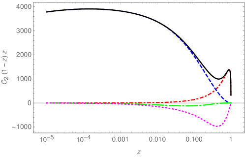
Figure 2: The initial state $O(\alpha^{2})$ corrections to $\gamma^{*}/Z^{*}$ production due to $e^{+}e^{-}$ pair production multiplied by $z(1-z)$. The non–singlet contribution (process II): dash-dotted line; the pure singlet contribution (process III): dashes; the interference term between both contributions (process IV) $\times 10$: dotted; the vector contributions implied by process B, Ref. [38], and interferences $\times 100$: long dash-dotted; all contributions: full line for $s=M_{Z}^{2}$; from [9].

In the small $z$ region up to about $z\sim 0.2$ the pure singlet contribution dominates. For still larger values, the non–singlet contribution dominates and at intermediate values there is a negative contribution due to the interference terms of both. There is another contribution at $O(a^{2})$ having no logarithmic parts, which has not been considered in [2] but in [38], which is rather small. We would also like to mention that the radiative corrections are different for the vector–axial vector interference contributions if compared to the pure vector and pure axial vector contributions, which has been considered in Refs. [9, 11].

In this and the subsequent calculations reported in this survey we have extensively used the packages FORM [39] Sigma [40, 41], EvaluateMultiSum [42], HarmonicSums [43, 8, 49, 31, 44, 46, 47, 48, 45], HolonomicFunctions [50], and private implementations [30] to calculate the respective integrals analytically.

2.2 The Method of Massive Operator Matrix Elements

The method of massive operator matrix elements has been introduced in QCD to calculate heavy flavor corrections to deep–inelastic scattering at two–loop order for all but contributions due to power corrections of $O((m^{2}_{Q}/Q^{2})^{k}),k\geq 1$, with $Q^{2}$ the virtuality of the exchanged gauge boson and $m_{Q}$ the heavy quark mass [4]. It is also applicable to massive Drell–Yan processes as studied in the present paper and has been applied in [2], showing that it works at one–loop order and for all logarithmic contributions at two–loop order. However, there has not been a clear conclusion in [2], whether it works also for the non–logarithmic contribution at $O(a^{2})$. It has been found in [3], that the $O(a^{2})$ terms given in [2] are indeed not reproduced. For us it initially caused doubts on its inapplicability, because this factorization might not be present in the massive Drell–Yan process, although it is expected. The complete result obtained in Ref. [6], see Section 2.1, has then fully confirmed our earlier result in the factorized approach [3]. In the following we will outline the different steps in this approach in detail, also for later use at even higher orders [13], see Section 3.

The general decomposition of the scattering cross section in Mellin space is given by, cf. [3]

$$\frac{d\sigma_{e^{+}e^{-}}}{ds^{\prime}} = \frac{1}{s}\sigma^{(0)}(s^{\prime})\Biggl{[}\Gamma_{e^{+}e^{+}}\left(N,\frac{\mu^{2}}{m_{e}^{2}}\right)\tilde{\sigma}_{e^{+}e^{-}}\left(N,\frac{s^{\prime}}{\mu^{2}}\right)\Gamma_{e^{-}e^{-}}\left(N,\frac{\mu^{2}}{m_{e}^{2}}\right)$$ (21)

$$+\Gamma_{\gamma e^{+}}\left(N,\frac{\mu^{2}}{m_{e}^{2}}\right)\tilde{\sigma}_{e^{-}\gamma}\left(N,\frac{s^{\prime}}{\mu^{2}}\right)\Gamma_{e^{-}e^{-}}\left(N,\frac{\mu^{2}}{m_{e}^{2}}\right)$$

$$+\Gamma_{e^{+}e^{+}}\left(N,\frac{\mu^{2}}{m_{e}^{2}}\right)\tilde{\sigma}_{e^{+}\gamma}\left(N,\frac{s^{\prime}}{\mu^{2}}\right)\Gamma_{\gamma e^{-}}\left(N,\frac{\mu^{2}}{m_{e}^{2}}\right)$$

$$+\Gamma_{\gamma e^{+}}\left(N,\frac{\mu^{2}}{m_{e}^{2}}\right)\tilde{\sigma}_{\gamma\gamma}\left(N,\frac{s^{\prime}}{\mu^{2}}\right)\Gamma_{\gamma e^{-}}\left(N,\frac{\mu^{2}}{m_{e}^{2}}\right)\Biggr{]}.$$

The terms in the brackets $[...]$ are Mellin–convoluted. Only massive OMEs of the kind $\Gamma_{e^{\pm}e^{\pm}}$ and $\Gamma_{\gamma e^{\pm}}$ contribute because the process considered has electron–positron initial states and the $\tilde{\sigma}_{\gamma\gamma}$ terms appear only from $O(a^{4})$ onward. In the factorization also the massless Wilson coefficients for the Drell-Yan process $\tilde{\sigma}_{ij}$, $i,j=e^{\pm},\gamma$ contribute. The factorization scale $\mu$ cancels after expanding in $a_{0}=a(m_{e}^{2})$. The following expansions hold for the massive OMEs and massless Wilson coefficients

$$\Gamma_{li}\left(N,\frac{\mu^{2}}{m_{e}^{2}}\right) = \delta_{li}+\sum_{r=1}^{\infty}a^{r}(\mu^{2})\sum_{n=0}^{r}a_{li;nr}(N)\Lambda^{n}$$ (22)

$$\tilde{\sigma}_{lk}\left(N,\frac{s^{\prime}}{\mu^{2}}\right) = \delta_{lk}+\sum_{r=1}^{\infty}a^{r}(\mu^{2})\sum_{n=0}^{r}b_{lk;nr}(N)\lambda^{n},$$ (23)

with the logarithms $\Lambda$ and $\lambda$ given by

$$\Lambda=\ln\left(\frac{\mu^{2}}{m_{e}^{2}}\right),\leavevmode\nobreak\ \leavevmode\nobreak\ \leavevmode\nobreak\ \leavevmode\nobreak\ \leavevmode\nobreak\ \leavevmode\nobreak\ \leavevmode\nobreak\ \lambda=\ln\left(\frac{s^{\prime}}{\mu^{2}}\right).$$ (24)

The massive OMEs $\Gamma_{ij}$ and massless Wilson coefficients $\tilde{\sigma}_{kl}$ fulfill the following renormalization group equations, cf. [51],

$$\left[\left(\frac{\partial}{\partial\Lambda}+\beta(a)\frac{\partial}{\partial a}\right)\delta_{kl}+\frac{1}{2}\gamma_{kl}(N,a)\right]\Gamma_{li}\left(N,a,\frac{\mu^{2}}{m_{e}^{2}}\right) = 0$$ (25)

$$\left[\left(\frac{\partial}{\partial\lambda}-\beta(a)\frac{\partial}{\partial a}\right)\delta_{kl}\delta_{jm}+\frac{1}{2}\gamma_{kl}(N,a)\delta_{jm}+\frac{1}{2}\gamma_{jm}(N,a)\delta_{kl}\right]\tilde{\sigma}_{lj}\left(N,a,\frac{s^{\prime}}{\mu^{2}}\right) = 0\leavevmode\nobreak\ ,$$ (26)

and the QED $\beta$ function has the representation

$$\beta(a)=-\sum_{k=0}^{\infty}\beta_{k}a^{k+2},$$ (27)

with $\beta_{0}=-4/3,\leavevmode\nobreak\ \beta_{1}=-4$.

The calculation of the scattering cross section (21) to $O(a_{0}^{2})$ requires the knowledge of the expansion coefficients of the massless Drell–Yan cross section [38, 54, 9] to $O(a_{0}^{2})$, the one– and two–loop anomalous dimensions $\gamma_{ij}^{(k)}$ [55], and the massive OMEs $\Gamma_{ee}^{(0)},\Gamma_{e\gamma}^{(0)}$ and $\Gamma_{ee}^{(1)}$. The latter quantity needs to be known in its contributions to processes i) + iv), ii) and iii). The major task in Ref. [3] has been to calculate $\Gamma_{ee}^{(1)}$. At that time, many of the automated methods and function spaces found in later massive calculations have been not yet known, cf. [56], and majorly hypergeometric integration techniques [57] were used. Checks have been performed using the package tarcer [58] and detailed lists of special integrals had to be calculated, cf. [3].

As an example, we show the massive OME $\hat{\hat{A}}_{ee}^{\rm III}$, from which $\Gamma_{ee}^{\rm III}$ is obtained,

$$\hat{\hat{A}}_{ee}^{(2),\rm III} = S_{\varepsilon}^{2}\int^{1}_{0}dx\,\,x^{N}\frac{1+(-1)^{N}}{2}\left\{\phantom{\rule{0.28453pt}{16.21828pt}}\!\right.\frac{8}{\varepsilon^{2}}\left[\frac{1-x}{3x}(4x^{2}+7x+4)+2(1+x)\ln(x)\right]$$ (28)

$$\phantom{\int^{1}_{0}dx\,\,x^{n}\left\{\phantom{\rule{0.28453pt}{16.21828pt}}\!\right.}+\frac{4}{\varepsilon}\left[\phantom{\rule{0.28453pt}{15.93347pt}}\!\right.5(1+x)\ln^{2}(x)-\frac{1+x}{3x}(8x^{2}-17x-16)\ln(x)+\frac{4(1-x)}{9x}(5x^{2}$$

$$\phantom{\int^{1}_{0}dx\,\,x^{n}\left\{\phantom{\rule{0.28453pt}{16.21828pt}}\!\right.}+23x+14)\left.\!\phantom{\rule{0.28453pt}{15.93347pt}}\right]+\frac{2}{x}(1-x)(4x^{2}+13x+4)\zeta_{2}+\frac{1}{3x}(8x^{3}+135x^{2}+75x$$

$$\phantom{\int^{1}_{0}dx\,\,x^{n}\left\{\phantom{\rule{0.28453pt}{16.21828pt}}\!\right.}+32)\ln^{2}(x)+\left[\frac{304}{9x}-\frac{80}{9}x^{2}-\frac{32}{3}x+108-\frac{32}{1+x}-\frac{64(1+2x)}{3(1+x)^{3}}\right]\ln(x)$$

$$\phantom{\int^{1}_{0}dx\,\,x^{n}\left\{\phantom{\rule{0.28453pt}{16.21828pt}}\!\right.}-\frac{224}{27}x^{2}+16\frac{1-x}{3x}(x^{2}+4x+1)\left[2\ln(x)\ln(1+x)-{\rm Li}_{2}(1-x)\right.$$

$$\phantom{\int^{1}_{0}dx\,\,x^{n}\left\{\phantom{\rule{0.28453pt}{16.21828pt}}\!\right.}\left.+2{\rm Li}_{2}(-x)\right]+(1+x)\left[\phantom{\rule{0.28453pt}{15.93347pt}}\!\right.4\zeta_{2}\ln(x)+\frac{14}{3}\ln^{3}(x)-32\ln(x){\rm Li}_{2}(-x)$$

$$\phantom{\int^{1}_{0}dx\,\,x^{n}\left\{\phantom{\rule{0.28453pt}{16.21828pt}}\!\right.}-16\ln(x){\rm Li}_{2}(x)+64{\rm Li}_{3}(-x)+32{\rm Li}_{3}(x)+16\zeta_{3}\left.\!\phantom{\rule{0.28453pt}{15.93347pt}}\right]-\frac{182}{3}x+50$$

$$\phantom{\int^{1}_{0}dx\,\,x^{n}\left\{\phantom{\rule{0.28453pt}{16.21828pt}}\!\right.}-\frac{32}{1+x}+\frac{800}{27x}+\frac{64}{3(1+x)^{2}}\left.\!\phantom{\rule{0.28453pt}{15.93347pt}}\right\}m_{e}^{2\varepsilon}(\Delta\cdot p)^{N}\leavevmode\nobreak\ .$$

Here $\Delta$ is a light–like vector, $p$ the external momentum of the OME, $N$ labels the Mellin moment, $\varepsilon=D-4$ is the dimensional parameter, and $S_{\varepsilon}=\exp[(\varepsilon/2)(\gamma_{E}-\ln(4\pi))]$ is the spherical factor, with $\gamma_{E}$ the Euler–Mascheroni constant.

After all building blocks which enter (21) have been calculated, one can perform the corresponding Mellin transforms analytically and obtain all the radiators, which were also obtained in the direct calculation, presented in Section 2.1.

2.3 Numerical Results at $O(\alpha^{2})$

The initial state QED corrections can be written in terms of the radiator functions introduced in Section 2.1, which we use in the following to calculate the ISR corrections to different processes.

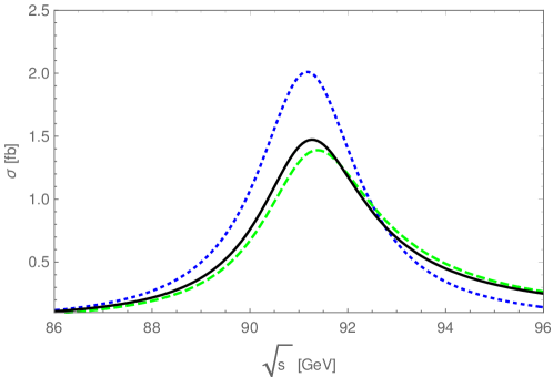
Figure 3: The $Z$-resonance in $e^{+}e^{-}\rightarrow\mu^{+}\mu^{-}$. Dotted line: Born cross section; Dashed line: $O(\alpha)$ ISR corrections; Full line: $O(\alpha^{2})$ + soft resummation ISR corrections, with $s_{0}=4m_{\tau}^{2}$; from Ref. [12].

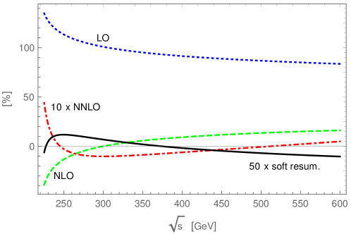
Figure 4: Relative contributions of the ISR QED corrections to the cross section for $e^{+}e^{-}\rightarrow ZH$ in %. Dotted line: $O(\alpha^{0})$; Dashed line: $O(\alpha)$; Dash-dotted line: $O(\alpha^{2})$; Full line: soft resummation beyond $O(\alpha^{2})$, with $s_{0}=4m_{\tau}^{2}$; from Ref. [12].

Here we consider the contribution to $O(\alpha^{2})$ only and turn to higher order corrections in Section 3. We discuss the ISR corrections for the $Z$ peak and its surrounding, the process $e^{+}e^{-}\rightarrow ZH$, and $t\bar{t}$ production in the threshold region, cf. Ref. [12]. The ISR corrections depend on the experimental cut $s_{0}$. In the LEP1 analysis it has been chosen $s_{0}=4m_{\tau}^{2}$ or $s_{0}=0.01M_{Z}^{2}$ [1]. Furthermore, one considers the cases of a fixed $Z$-width or the $s$-dependent $Z$-width, leading to a peak shift of $34.2$ MeV and a shift of the width of 1 MeV, in accordance with Refs. [59]. We illustrate the different QED ISR corrections to $e^{+}e^{-}\rightarrow Z^{*}/\gamma^{*}$ around the $Z$ peak in Figure 3. The ISR corrections change the profile of the resonance, i.e. the peak position, height and the half width. The effect of soft resummation beyond $O(\alpha^{2})$ are nearly invisible.

More detailed effects, also due to higher order corrections, are discussed in Table 1 in Section 3. The new results, compared with [2], imply a relative shift in the $Z$-width by $\sim$4 MeV for $s_{0}=4m_{\tau}^{2}$, being larger than the current value of $\Delta\Gamma_{Z}=\pm 2.3$ MeV [60], which may require a reanalysis of the LEP data to obtain consistent results.

For the study of the radiative corrections to the process $e^{+}e^{-}\rightarrow ZH$ we refer to the Born cross section in [61]. The anticipated experimental accuracy for this process should reach 1% [62] at future colliders like the ILC, CLIC, and even $0.4\%$ at the FCC_ee [63]. Figure 4 shows the relative corrections of ISR corrections.

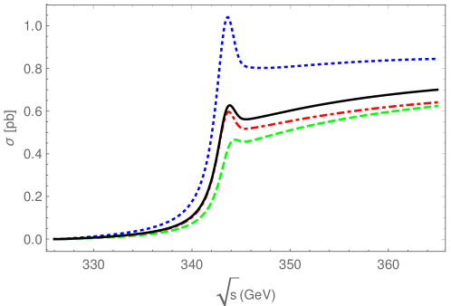
Figure 5: The QED ISR corrections to $e^{+}e^{-}\rightarrow t\overline{t}$ ($s$-channel photon exchange) in the threshold region for a PS-mass of $m_{t}=172\leavevmode\nobreak\ \mathrm{GeV}$. Dotted line $O(\alpha^{0})$; Dashed line $O(\alpha)$; Dash-dotted line $O(\alpha^{2})$; Full line $O(\alpha^{2})$ + soft resummation; from Ref. [12].

The NNLO corrections vary between +4.8% and $-1\%$ and are thus larger or of the size of the expected experimental errors, which might imply the need of higher order corrections. On the other hand, the soft resummation contributions are of $O(\pm 0.2\%)$ and reach half of the projected accuracy.

The QED corrections to $t\bar{t}$ production in the threshold region are shown in Figure 5. For the cross section at threshold we use the N³LO QCD corrections implemented in the code QQbar_threshold [64, 65, 66] without QED corrections. Figure 5 illustrates the convergence of the corrections from the uncorrected cross section to the one with the $O(\alpha^{2})$ corrections and higher order soft resummation, which is stable up to the peak region an displays still some shift towards the continuum region. Accuracy studies for this process have been made in Refs. [67, 68].

The full two–loop QED corrections are mandatory down to the constant contribution to match the anticipated experimental accuracy for key processes to be measured at future $e^{+}e^{-}$ colliders and they were mandatory in the analysis of the LEP experiments. Given the luminosity projected for future experiments, even higher order corrections will become necessary, to which we turn now.

3 The Higher Order Corrections

In the previous section it has been shown, that the method of massive OMEs provides an equivalent way to calculate the initial state corrections in the limit $m_{e}^{2}/s\rightarrow 0$. This is fully justified in particular for inclusive calculations, where the power corrections being neglected do not play any role as e.g. in high energy electron-positron collisions. However, the constant part is still important. One arrives at hierarchies of the kind $O(\alpha^{k}L^{k}),O(\alpha^{k}L^{k-1}),O(\alpha^{k}L^{k-2}),...,O(\alpha^{k})$. By using the renormalization group equation one can now derive three consecutive corrections, for which all massive OMEs are available together with the two–loop corrections to the massless Drell–Yan cross section [38, 54, 9]. In Ref. [13] we have calculated all the corresponding corrections up to $O(\alpha^{6}L^{5})$.

To obtain the leading logarithmic contributions to the radiators we solve (21) to the desired order and calculate the coefficients of the expansion of the inclusive radiator given in Eqs. (1,2) in Mellin space. While at lower orders all terms are obtained, at three–loop order we get the coefficients $c_{3,3},c_{3,2}$ and $c_{3,1}$ only, etc. For example we obtain

$$c_{3,1} = -\gamma_{ee}^{(2)}-2\Gamma_{ee}^{(0)}\gamma_{ee}^{(1)}-\Gamma_{ee}^{(0)}\gamma_{e\gamma}^{(0)}\Gamma_{\gamma e}^{(0)}-\gamma_{e\gamma}^{(1)}\Gamma_{\gamma e}^{(0)}-\gamma_{e\gamma}^{(0)}\Gamma_{\gamma e}^{(1)}-\beta_{1}\sigma_{ee}^{(0)}-\gamma_{ee}^{(1)}\sigma_{ee}^{(0)}$$ (29)

$$-\gamma_{e\gamma}^{(0)}\Gamma_{\gamma e}^{(0)}\sigma_{ee}^{(0)}-2\Gamma_{ee}^{(0)}\gamma_{\gamma e}^{(0)}\sigma_{e\gamma}^{(0)}-\gamma_{\gamma e}^{(1)}\sigma_{e\gamma}^{(0)}-\Gamma_{\gamma e}^{(0)}\gamma_{\gamma\gamma}^{(0)}\sigma_{e\gamma}^{(0)}-\gamma_{\gamma e}^{(0)}\sigma_{\gamma e}^{(1)}+\beta_{0}\Bigl{[}-2\Gamma_{ee}^{(0)}\sigma_{ee}^{(0)}$$

$$-2\sigma_{ee}^{(1)}-2\Gamma_{\gamma e}^{(0)}\sigma_{e\gamma}^{(0)}\Bigr{]}-\gamma_{ee}^{(0)}\left[{\Gamma_{ee}^{(0)}}^{2}+2\Gamma_{ee}^{(1)}+2\Gamma_{ee}^{(0)}\sigma_{ee}^{(0)}+\sigma_{ee}^{(1)}+\Gamma_{\gamma e}^{(0)}\sigma_{e\gamma}^{(0)}\right].$$

The calculation is best carried out in Mellin space and the $z$–space representation is finally obtained by an analytic Mellin inversion using the tools of the package HarmonicSums.

As can be seen from Eq. (29), starting with three–loop order the expansion coefficient $\Gamma_{\gamma e}^{(1)}$ contributes. In Mellin space it is obtained from the massive OME $A_{\gamma e}^{(2)}$, cf. [13],

$$A_{\gamma e}^{(2)}(N) = \Biggl{[}\frac{\big{(}N^{2}+N+2\big{)}\big{(}N^{2}+N+6\big{)}}{3(N-1)N^{2}(N+1)^{2}}-\frac{4\big{(}N^{2}+N+2\big{)}}{(N-1)N(N+1)}S_{1}\Biggr{]}L^{2}$$ (30)

$$-\Biggl{[}\frac{2P_{2}}{9(N-1)^{2}N^{3}(N+1)^{3}}-\frac{4P_{1}}{3(N-1)N^{2}(N+1)^{2}}S_{1}+\frac{12\big{(}N^{2}+N+2\big{)}}{(N-1)N(N+1)}S_{1}^{2}$$

$$+\frac{12\big{(}N^{2}+N+2\big{)}}{(N-1)N(N+1)}S_{2}\Biggr{]}L+\frac{P_{8}}{27(N-4)(N-3)(N-2)(N-1)N^{4}(N+1)^{4}}$$

$$+\biggl{(}\frac{2P_{7}}{9(N-4)(N-3)(N-2)(N-1)N^{3}(N+1)^{3}}+\frac{2\big{(}N^{2}+N+2\big{)}}{(N-1)N(N+1)}S_{2}\biggr{)}S_{1}$$

$$+\frac{P_{3}}{3(N-2)(N-1)N(N+1)^{2}}S_{1}^{2}+\frac{2\big{(}N^{2}+N+2\big{)}}{3(N-1)N(N+1)}S_{1}^{3}$$

$$+\frac{P_{6}}{3(N-2)(N-1)N^{2}(N+1)^{2}}S_{2}+\frac{4\big{(}N^{2}+N+2\big{)}}{3(N-1)N(N+1)}S_{3}$$

$$-\frac{48\big{(}N^{2}+N+2\big{)}}{(N-1)N(N+1)}S_{2,1}+\frac{3\cdot 2^{6+N}}{(N-2)(N+1)^{2}}S_{1,1}\biggl{(}\frac{1}{2},1\biggr{)}$$

$$+\frac{2^{6-N}P_{5}}{3(N-3)(N-2)(N-1)^{2}N^{2}}\biggl{(}S_{2}(2)+S_{1}S_{1}(2)-S_{1,1}(1,2)-S_{1,1}(2,1)\biggr{)}$$

$$-\frac{32\big{(}N^{2}+N+2\big{)}}{(N-1)N(N+1)}\biggl{[}S_{1}(2)S_{1,1}\biggl{(}\frac{1}{2},1\biggr{)}+S_{1,2}\biggl{(}\frac{1}{2},2\biggr{)}-S_{1,1,1}\biggl{(}\frac{1}{2},1,2\biggr{)}$$

$$-S_{1,1,1}\biggl{(}\frac{1}{2},2,1\biggr{)}-\frac{\zeta_{2}}{2}S_{1}(2)\biggr{]}+\frac{4P_{4}}{(N-2)(N-1)N^{2}(N+1)^{2}}\zeta_{2},$$

with the polynomials

$$P_{1} = 25N^{4}+44N^{3}+87N^{2}+56N+12,$$ (31)

$$P_{2} = 112N^{7}+194N^{6}+347N^{5}+339N^{4}+93N^{3}-293N^{2}-60N+36,$$ (32)

$$P_{3} = 17N^{4}-66N^{3}-179N^{2}-272N-212,$$ (33)

$$P_{4} = N^{5}+4N^{4}+25N^{3}+14N^{2}+12N+8-3\cdot 2^{N+3}N^{2}\bigl{(}N-1\bigr{)},$$ (34)

$$P_{5} = 9N^{5}-24N^{4}+8N^{3}+4N^{2}+33N-18,$$ (35)

$$P_{6} = 11N^{5}-90N^{4}-329N^{3}-356N^{2}-284N-48,$$ (36)

$$P_{7} = 17N^{9}+213N^{8}-1729N^{7}+2329N^{6}-5196N^{5}+7898N^{4}+16196N^{3}$$ (37)

$$+12528N^{2}-4896N-3456,$$

$$P_{8} = -509N^{11}+2365N^{10}+2797N^{9}-13158N^{8}+31274N^{7}-4694N^{6}-64636N^{5}$$ (38)

$$-107861N^{4}-14622N^{3}+6588N^{2}-2376N-2592.$$

The radiators are obtained in terms of harmonic sums [46, 47] and generalized harmonic sums [31] or harmonic polylogarithms [48] $H_{\vec{a}}(z)$ and $H_{\vec{a}}(1-z)$ weighted by rational coefficients. The choice of arguments has been made to avoid the occurrence of more general iterated integrals. As usual, the radiators in $z$-space are distribution valued. We show the coefficient $c_{3,1}$ in Mellin space as an example,

$$c_{3,1} = \Biggl{\{}\frac{\big{(}2+N+N^{2}\big{)}2^{8-N}[S_{2}(2)-S_{1,1}(1,2)-S_{1,1}(2,1)]Q_{36}}{3(N-3)(N-2)(N-1)^{2}N^{3}(N+1)(N+2)}$$ (39)

$$+\frac{16S_{2,1}Q_{54}}{9(N-1)N^{2}(N+1)^{2}(N+2)}+\frac{8S_{3}Q_{91}}{27(N-1)N^{2}(N+1)^{2}(N+2)}$$

$$+\frac{Q_{206}}{81(N-4)(N-3)(N-2)(N-1)^{2}N^{5}(N+1)^{5}(N+2)^{3}}$$

$$+\Biggl{[}\Biggl{[}-\frac{64S_{1}Q_{119}}{3(N-1)N^{2}(N+1)^{2}(N+2)^{2}}+\frac{32Q_{144}}{9(N-1)N^{3}(N+1)^{3}(N+2)^{2}}$$

$$+\frac{768(N+3)\big{(}2+N^{2}\big{)}S_{1}^{2}}{(N-1)N(N+1)(N+2)}\Biggr{]}S_{-2}+\Biggl{[}-\frac{32(N+3)\big{(}2+N^{2}\big{)}\big{(}6+13N+13N^{2}\big{)}}{3(N-1)N^{2}(N+1)^{2}(N+2)}$$

$$+\frac{128(N+3)\big{(}2+N^{2}\big{)}S_{1}}{(N-1)N(N+1)(N+2)}\Biggr{]}S_{-3}+\frac{64(N+3)\big{(}2+N^{2}\big{)}\big{(}6+13N+13N^{2}\big{)}S_{-2,1}}{(N-1)N^{2}(N+1)^{2}(N+2)}$$

$$-\frac{768(N+3)\big{(}2+N^{2}\big{)}S_{1}S_{-2,1}}{(N-1)N(N+1)(N+2)}+\Biggl{[}-\frac{32S_{1}Q_{119}}{3(N-1)N^{2}(N+1)^{2}(N+2)^{2}}$$

$$+\frac{16Q_{144}}{9(N-1)N^{3}(N+1)^{3}(N+2)^{2}}+\frac{384(N+3)\big{(}2+N^{2}\big{)}S_{1}^{2}}{(N-1)N(N+1)(N+2)}\Biggr{]}\zeta_{2}$$

$$+\Biggl{[}\frac{32(N+3)\big{(}2+N^{2}\big{)}\big{(}6+13N+13N^{2}\big{)}}{(N-1)N^{2}(N+1)^{2}(N+2)}-\frac{384(N+3)\big{(}2+N^{2}\big{)}S_{1}}{(N-1)N(N+1)(N+2)}\Biggr{]}\zeta_{3}\Biggr{]}(-1)^{N}$$

$$+\Biggl{[}-\frac{64S_{2,1}Q_{6}}{3(N-1)N(N+1)}+\frac{\big{(}2+N+N^{2}\big{)}2^{8-N}S_{1}(2)Q_{36}}{3(N-3)(N-2)(N-1)^{2}N^{3}(N+1)(N+2)}$$

$$-\frac{64S_{3}Q_{20}}{9(N-1)N}-\frac{16S_{2}Q_{132}}{27(N-1)N^{2}(N+1)^{2}(N+2)^{2}}$$

$$-\frac{8Q_{201}}{81(N-4)(N-3)(N-2)(N-1)^{2}N^{4}(N+1)^{4}(N+2)^{3}}-1152S_{2}^{2}-384S_{4}$$

$$-1280S_{3,1}-1024S_{-2,-1}+768S_{2,1,1}\Biggr{]}S_{1}+\Biggl{[}\frac{32S_{2}Q_{8}}{(N-1)N(N+1)}-256S_{2,1}$$

$$+\frac{16Q_{150}}{27(N-2)(N-1)^{2}N^{3}(N+1)^{3}(N+2)^{2}}\Biggr{]}S_{1}^{2}+\Biggl{[}-\frac{64Q_{40}}{27(N-1)N^{2}(N+1)^{2}(N+2)}$$

$$-128S_{2}\Biggr{]}S_{1}^{3}+\frac{512}{9}S_{1}^{4}+\Biggl{[}\frac{4Q_{175}}{27(N-2)(N-1)^{2}N^{3}(N+1)^{3}(N+2)^{2}}-384S_{3}\Biggr{]}S_{2}$$

$$+\frac{32\big{(}54+97N+97N^{2}\big{)}S_{2}^{2}}{3N(N+1)}+\frac{32(2+5N)(3+5N)S_{4}}{N(N+1)}+384S_{5}$$

$$+\Biggl{[}\Biggl{[}-\frac{256\big{(}2+3N+3N^{2}\big{)}}{N(N+1)}+1024S_{1}\Biggr{]}S_{-1}-256S_{-2,1}\Biggr{]}S_{-2}+640S_{-3}S_{-2}+192S_{-2}^{2}$$

$$+\frac{64\big{(}30+11N+11N^{2}\big{)}S_{3,1}}{3N(N+1)}-384S_{3,2}-384S_{4,1}+\frac{256\big{(}2+3N+3N^{2}\big{)}S_{-2,-1}}{N(N+1)}$$

$$-\frac{64\big{(}6+11N+11N^{2}\big{)}S_{2,1,1}}{N(N+1)}+768S_{3,1,1}-1024S_{-2,1,-2}$$

$$+\frac{3\big{(}2+N+N^{2}\big{)}2^{8+N}S_{1,1}\big{(}\frac{1}{2},1\big{)}}{(N-2)N(N+1)^{3}(N+2)}-\frac{128\big{(}2+N+N^{2}\big{)}^{2}S_{1}(2)S_{1,1}\big{(}\frac{1}{2},1\big{)}}{(N-1)N^{2}(N+1)^{2}(N+2)}$$

$$-\frac{128\big{(}2+N+N^{2}\big{)}^{2}(S_{1,2}\big{(}\frac{1}{2},2\big{)}-S_{1,1,1}\big{(}\frac{1}{2},1,2\big{)}-S_{1,1,1}\big{(}\frac{1}{2},2,1\big{)})}{(N-1)N^{2}(N+1)^{2}(N+2)}$$

$$+\Biggl{[}-\frac{32S_{1}^{2}Q_{12}}{3(N-1)N(N+1)}-\frac{4Q_{174}}{27(N-2)(N-1)^{2}N^{3}(N+1)^{3}(N+2)^{2}}$$

$$+\ln(2)\Biggl{[}-\frac{576\big{(}2+3N+3N^{2}\big{)}}{N(N+1)}+2304S_{1}\Biggr{]}$$

$$+128S_{1}^{3}+\Biggl{[}\frac{16Q_{133}}{27(N-1)N^{2}(N+1)^{2}(N+2)^{2}}+2432S_{2}\Biggr{]}S_{1}-\frac{64\big{(}19+30N+30N^{2}\big{)}S_{2}}{N(N+1)}$$

$$+576S_{3}+\Biggl{[}-\frac{128\big{(}2+3N+3N^{2}\big{)}}{N(N+1)}+512S_{1}\Biggr{]}S_{-1}+192S_{-2}+320S_{-3}$$

$$-640S_{-2,1}+\frac{64\big{(}2+N+N^{2}\big{)}^{2}S_{1}(2)}{(N-1)N^{2}(N+1)^{2}(N+2)}+160\zeta_{3}\Biggr{]}\zeta_{2}$$

$$+\Biggl{[}\frac{16\big{(}588+1171N+1171N^{2}\big{)}}{15N(N+1)}-\frac{6272}{5}S_{1}\Biggr{]}\zeta_{2}^{2}+\Biggl{[}\frac{64S_{1}Q_{34}}{3(N-1)N(N+1)}+512S_{1}^{2}$$

$$-\frac{16Q_{85}}{9(N-1)N^{2}(N+1)^{2}(N+2)}-192S_{2}+192S_{-2}\Biggr{]}\zeta_{3}-416\zeta_{5}\Biggr{\}},$$

with $Q_{i}$ polynomials in $N$, cf. [13].

The numerical effect of the corrections of up to $O(\alpha^{6}L^{5})$ are illustrated in Table 1 describing the $Z^{0}$-peak both in the case of a fixed width and the $s$ dependent width. The radiative corrections change both the peak positions and the width. The corrections due to the different orders may be positive or negative. We list the individual contributions.

At $O(\alpha^{6}L^{6})$ the corrections to the peak are 7 keV and to the width 27 keV. The next subleading correction serves as a control term. For measurements at the future FCC_ee statistical accuracies of $\Delta M_{Z}=50\leavevmode\nobreak\ \mathrm{keV}\leavevmode\nobreak\ {\rm[stat]},\Delta\Gamma_{Z}=8\leavevmode\nobreak\ \mathrm{keV}\leavevmode\nobreak\ {\rm[stat]}$ are estimated [69]. This precision level is about reached in the case of the present corrections. In the case a further logarithmic order is needed, one needs to calculated both, one more order for the Drell–Yan process and one more for the massive OMEs. Furthermore, the electro–weak corrections and QCD corrections have to be pushed to higher orders. All of this will meet theoretical and technological (i.e. mathematical and computer–algebraic) challenges.

	Fixed width		$s$ dep. width
	Peak	Width	Peak	Width
	(MeV)	(MeV)	(MeV)	(MeV)
$O(\alpha)$ correction	185.638	539.408	181.098	524.978
$O(\alpha^{2}L^{2})$:	– 96.894	–177.147	– 95.342	–176.235
$O(\alpha^{2}L)$:	6.982	22.695	6.841	21.896
$O(\alpha^{2})$:	0.176	– 2.218	0.174	– 2.001
$O(\alpha^{3}L^{3})$:	23.265	38.560	22.968	38.081
$O(\alpha^{3}L^{2})$:	– 1.507	– 1.888	– 1.491	– 1.881
$O(\alpha^{3}L)$:	– 0.152	0.105	– 0.151	– 0.084
$O(\alpha^{4}L^{4})$:	– 1.857	0.206	– 1.858	0.146
$O(\alpha^{4}L^{3})$:	0.131	– 0.071	0.132	– 0.065
$O(\alpha^{4}L^{2})$:	0.048	– 0.001	0.048	0.001
$O(\alpha^{5}L^{5})$:	0.142	– 0.218	0.144	– 0.212
$O(\alpha^{5}L^{4})$:	– 0.000	0.020	– 0.001	0.020
$O(\alpha^{5}L^{3})$:	– 0.008	0.009	– 0.008	0.008
$O(\alpha^{6}L^{6})$:	– 0.007	0.027	– 0.007	0.027
$O(\alpha^{6}L^{5})$:	– 0.001	0.000	– 0.001	0.000

Table 1: Shifts in the $Z$-mass and the width due to the different contributions to the ISR QED radiative corrections for a fixed width of $\Gamma_{Z}=2.4952\leavevmode\nobreak\ \mathrm{GeV}$ and $s$-dependent width using $M_{Z}=91.1876\leavevmode\nobreak\ \mathrm{GeV}$ [60] and $s_{0}=4m_{\tau}^{2}$, cf. [1]; from [13].

The method of massive OMEs has been also applied to calculate the massive Wilson coefficients for deep inelastic scattering in the region $Q^{2}\gg m_{Q}^{2}$ in the single and two–mass cases at three–loop order analytically in Refs. [70].

4 The Forward-Backward Asymmetry

A high luminosity measurement of the forward–backward asymmetry provides an excellent possibility for a precision measurement of the fine structure constant at high energy [71]. This is important because of its hadronic contributions [72]. The calculation of the forward–backward asymmetry at one–loop order has been performed in [73, 79, 78, 80, 74, 75, 76, 77], and the leading logarithmic two–loop corrections were computed in [79]. More recently the leading logarithmic contributions to $O(\alpha^{6}L^{6})$ have been calculated in Ref. [14]. Also the initial–final state interference terms, final state corrections, electro–weak and QCD corrections are known at lower orders, cf. [14].

The forward–backward asymmetry is defined as ratio over the difference and the sum of the angular integrals over the respective hemispheres measuring the final state muons,

$$\sigma_{F}=2\pi\int\limits_{0}^{1}{\rm d}\cos(\theta)\frac{{\rm d}\sigma}{{\rm d}\Omega},\leavevmode\nobreak\ \leavevmode\nobreak\ \leavevmode\nobreak\ \leavevmode\nobreak\ \leavevmode\nobreak\ \leavevmode\nobreak\ \sigma_{B}=2\pi\int\limits_{-1}^{0}{\rm d}\cos(\theta)\frac{{\rm d}\sigma}{{\rm d}\Omega}\,.$$ (40)

The angle $\theta$ is defined between the incoming electron $e^{-}$ and the outgoing muon $\mu^{-}$ from $\gamma^{*}/Z^{*}$ decay, with

$$A_{\text{FB}}(s) = \frac{\sigma_{F}(s)-\sigma_{B}(s)}{\sigma_{T}(s)},$$ (41)

and $\sigma_{T}(s)=\sigma_{F}(s)+\sigma_{B}(s)$. At Born level this reduces to [29]

$$\sigma_{\rm FB}^{(0)}(s) = \sigma_{F}^{(0)}(s)-\sigma_{B}^{(0)}(s)=\frac{\pi\alpha^{2}}{s}N_{C,f}\left(1-\frac{4m_{f}^{2}}{s}\right)G_{3}(s)\,,$$ (42)

$$\sigma_{T}^{(0)}(s) = \sigma_{F}^{(0)}(s)+\sigma_{B}^{(0)}(s)=\frac{4\pi\alpha^{2}}{3s}N_{C,f}\sqrt{1-\frac{4m_{f}^{2}}{s}}\left[\left(1+\frac{2m_{f}^{2}}{s}\right)G_{1}(s)-6\frac{m_{f}^{2}}{s}G_{2}(s)\right],$$

with $m_{f}$ the final state fermion mass, $m_{f}\equiv m_{\mu}$ and

$$G_{3}(s) = 2Q_{e}Q_{f}a_{e}a_{f}{\sf Re}[\chi_{Z}(s)]+4v_{e}v_{f}a_{e}a_{f}|\chi_{Z}(s)|^{2}.$$ (44)

The initial state corrections to $A_{\rm FB}$ at leading logarithmic level are described by two radiator functions $H_{e}^{LL}$ and $H_{FB}^{LL}$ [79], using the notation in [73],

$$A_{\text{FB}}(s) = \frac{1}{\sigma_{T}(s)}\int\limits_{z_{0}}^{1}{\rm d}z\,\frac{4z}{(1+z)^{2}}\tilde{H}_{e}^{LL}(z)\sigma_{\rm FB}^{(0)}(zs),\leavevmode\nobreak\ \leavevmode\nobreak\ \leavevmode\nobreak\ \leavevmode\nobreak\ \leavevmode\nobreak\ \leavevmode\nobreak\ \sigma_{T}(s)=\int\limits_{z_{0}}^{1}{\rm d}z\,H_{e}(z)\sigma_{T}^{(0)}(zs)\,,$$ (45)

with

$$\tilde{H}_{e}^{LL}(z)=\left[H_{e}^{LL}(z)+H_{FB}^{LL}(z)\right],$$ (46)

where the parameter $z_{0}$ plays the role of an energy cut and $z=s^{\prime}/s$. Here $H_{e}^{LL}$ is angular independent, and denotes the leading logarithmic contributions of the radiators of Section 2, while $H_{FB}^{LL}$ is angular dependent and obtained by the following integral

$$H_{FB}^{LL}(z)=\int\limits_{0}^{1}{\rm d}x_{1}\int\limits_{0}^{1}{\rm d}x_{2}\left(\frac{(1+z)^{2}}{(x_{1}+x_{2})^{2}}-1\right)\Gamma_{ee}^{LL}(x_{2})\Gamma_{ee}^{LL}(x_{1})\delta(x_{1}x_{2}-z).$$ (47)

Here $\Gamma_{ee}^{LL}(x_{i})$ denote the massive operator matrix elements and (47) is expanded in $(\alpha L)$ to the desired order. It is convenient to consider first the Mellin–transform

$$\mathcal{M}[H_{FB}^{LL}(z)](n) = \int\limits_{0}^{1}{\rm d}zz^{n}H_{FB}^{LL}(z)=\int\limits_{0}^{1}{\rm d}x_{1}\int\limits_{0}^{1}{\rm d}x_{2}x_{1}^{n}x_{2}^{n}\left(\frac{(1+x_{1}x_{2})^{2}}{(x_{1}+x_{2})^{2}}-1\right)\Gamma_{ee}^{LL}(x_{2})\Gamma_{ee}^{LL}(x_{1})$$

and to calculate the generating function

$$\mathcal{G}[H_{FB}^{LL}(z)](t) = \sum\limits_{n=0}^{\infty}t^{n}\mathcal{M}[H_{FB}^{LL}(z)](n),$$ (49)

from which we then obtain the individual radiators. They can be expressed by harmonic and cyclotomic harmonic polylogarithms [49] over the alphabet

$$\mathfrak{A}=\left\{f_{0}=\frac{1}{z},f_{1}=\frac{1}{1-z},f_{-1}=\frac{1}{1+z},f_{\{4,0\}}=\frac{1}{1+z^{2}},f_{\{4,1\}}=\frac{z}{1+z^{2}}\right\}.$$ (50)

$H_{FB}^{LL}$ starts at $O(\alpha^{2}L^{2})$.

	$A_{\rm FB}(s_{-})$	$A_{\rm FB}(M_{Z}^{2})$	$A_{\rm FB}(s_{+})$
$\mathcal{O}(\alpha^{0})$	$-0.3564803$	$0.0225199$	$0.2052045$
$\mathcal{O}(\alpha L^{1})$	$-0.2945381$	$-0.0094232$	$0.1579347$
$\mathcal{O}(\alpha L^{0})$	$-0.2994478$	$-0.0079610$	$0.1611962$
$\mathcal{O}(\alpha^{2}L^{2})$	$-0.3088363$	$0.0014514$	$0.1616887$
$\mathcal{O}(\alpha^{3}L^{3})$	$-0.3080578$	$0.0000198$	$0.1627252$
$\mathcal{O}(\alpha^{4}L^{4})$	$-0.3080976$	$0.0001587$	$0.1625835$
$\mathcal{O}(\alpha^{5}L^{5})$	$-0.3080960$	$0.0001495$	$0.1625911$
$\mathcal{O}(\alpha^{6}L^{6})$	$-0.3080960$	$0.0001499$	$0.1625911$

Table 2: $A_{\rm FB}$ evaluated at $s_{-}=(87.9\,{\rm GeV})^{2}$, $M_{Z}^{2}$ and $s_{+}=(94.3\,{\rm GeV})^{2}$ for the cut $z>4m_{\tau}^{2}/s$ from Ref. [14].

;

As an example $H_{FB}^{(3),LL}$ reads

$$H_{FB}^{(3),LL}(z) = -\frac{16(1-z)\big{(}4+11z+4z^{2}\big{)}}{3z}-\pi\biggl{[}\frac{4\big{(}2-3z-2z^{2}-3z^{3}+2z^{4}\big{)}}{3z^{3/2}}$$ (51)

$$+\frac{4(1-z)(1+5z)}{\sqrt{z}}H_{0}+\frac{16(1-z)^{2}}{\sqrt{z}}H_{\{4,1\}}\biggr{]}+\biggl{[}\frac{4(1+z)\big{(}5-18z-19z^{2}\big{)}}{3z}$$

$$-\frac{16(1-z)(1-7z)}{\sqrt{z}}H_{\{4,0\}}-96(1+z)H_{\{4,1\}}\biggr{]}H_{0}-8(1+z)H_{0}^{2}$$

$$+\biggl{[}\frac{16(1-z)(1+z)^{2}}{z}-\frac{64(1-z)^{2}}{\sqrt{z}}H_{\{4,0\}}\biggr{]}H_{1}+\biggl{[}\frac{16\big{(}2-3z-2z^{2}-3z^{3}+2z^{4}\big{)}}{3z^{3/2}}$$

$$+\frac{64(1-z)^{2}}{\sqrt{z}}H_{\{4,1\}}\biggr{]}H_{\{4,0\}}+\biggl{[}-\frac{16(1-z)(1+z)^{2}}{z}+64(1+z)H_{0}$$

$$+\frac{64(1-z)^{2}}{\sqrt{z}}H_{\{4,0\}}\biggr{]}H_{-1}-64(1+z)H_{0,1}+\frac{32(1-z)^{2}}{\sqrt{z}}H_{0,\{4,0\}}+96(1+z)H_{0,\{4,1\}}$$

$$+\frac{64(1-z)^{2}}{\sqrt{z}}H_{1,\{4,0\}}-\frac{64(1-z)^{2}}{\sqrt{z}}H_{\{4,0\},\{4,1\}}-64(1+z)H_{-1,0}$$

$$-\frac{64(1-z)^{2}}{\sqrt{z}}H_{-1,\{4,0\}}+20(1+z)\zeta_{2},$$

with $H_{\vec{w}}\equiv H_{\vec{w}}(\sqrt{z})$ and $\zeta_{k},k\in\mathbb{N},k\geq 2$ are the values of Riemann’s $\zeta$ function at integer argument.

Let us give some numerical illustration. We compute $A_{\rm FB}(s)$ for different values around the $Z^{0}$-peak as suggested in [71] to higher orders and see the corresponding improvement in Table 2. Comparing the results at one–loop to the highest order we obtain corrections of $-3$ % for $s_{-}$ and $-1\%$ for $s_{+}$. More numerical studies are presented in Ref. [14].

5 Conclusions

The precision calculations of the QED initial state corrections to the process $e^{+}e^{-}\rightarrow\gamma^{*}/Z^{*}$ are an essential ingredient for the planned key measurements at high energy $e^{+}e^{-}$ colliders such as the ILC, CLIC, FCC_ee, and future muon colliders. Due to the smallness of the ratio $m_{l}^{2}/s$, with $m_{l}$ the initial charged lepton mass, the logarithmic and constant term corrections in a massive environment are sufficient. It therefore has been important to clarify the differences between Ref. [2] and Ref. [3] at $O(a^{2})$. The differences found do in principle require to repeat the LEP electro–weak analysis, given the current accuracy of the $Z^{0}$ peak and width, because of the respective theoretical shifts. Since the codes TOPAZ0 [81, 80] and ZFITTER [82] contain the results of [2], they have to be updated for the use in further experimental analyses.

The agreement between Refs. [11] and [3] allowed to use the method of massive OMEs for even higher order corrections in the fine structure constant. Having available all OMEs which contribute at two–loop order, the first three logarithmic expansion coefficients are available through the renormalization group equations to any order in the fine structure constant, i.e. two further orders beyond the leading logarithmic approximation. The calculation of one more order seems to be technically possible. The presently available corrections reach the projected accuracies at the FCC_ee and need to be supplemented by corresponding QCD and electro–weak corrections.

For the forward–backward asymmetry, which might allow a precision measurement of the fine structure constant in the future, the leading logarithmic corrections have been extended to $O((\alpha L)^{6})$ and one might want to consider sub–leading corrections. Beyond the corrections in the leading logarithmic approximation, where harmonic sums are sufficient to express the radiators in Mellin space, one also finds generalized and cyclotomic harmonic sums, forming a part of the function spaces having been already revealed in other analytic massive single–scale calculations [56, 70]. We are still in the early phase to calculate the necessary radiative corrections for the high–luminosity measurements at the FCC_ee and will view more theoretical results during the decades ahead.

Acknowledgments.
We would like to thank A. De Freitas, W.L. van Neerven, and C.G. Raab for collaboration on the present topic and P. Janot and G. Passarino for discussions. This project has received funding from the European Union’s Horizon 2020 research and innovation programme under the Marie Sklodowska-Curie grant agreement No. 764850, SAGEX.

References

• [1] S. Schael et al., Phys. Rept.  427 (2006) 257–454 [hep-ex/0509008].
• [2] F.A. Berends, W.L. van Neerven and G.J.H. Burgers, Nucl. Phys. B 297 (1988) 429–478. Erratum: [Nucl. Phys. B 304 (1988) 921–922].
• [3] J. Blümlein, A. De Freitas and W.L. van Neerven, Nucl. Phys. B 855 (2012) 508–569 [arXiv:1107.4638 [hep-ph]].
• [4] M. Buza, Y. Matiounine, J. Smith, R. Migneron and W. L. van Neerven, Nucl. Phys. B 472 (1996) 611–658 [hep-ph/9601302].
• [5] B.A. Kniehl, M. Krawczyk, J.H. Kühn and R.G. Stuart, Phys. Lett. B 209 (1988) 337–342.
• [6] J. Blümlein, A. De Freitas, C.G. Raab and K. Schönwald, Nucl. Phys. B 945 (2019) 114659 [arXiv:1903.06155 [hep-ph]].
• [7] J. Blümlein, C.G. Raab and K. Schönwald, Nucl. Phys. B 948 (2019) 114736 [arXiv:1904. 08911 [hep-ph]].
• [8] J. Blümlein, Comput. Phys. Commun.  159 (2004) 19–54 [hep-ph/0311046].
• [9] J. Blümlein, A. De Freitas, C.G. Raab and K. Schönwald, Phys. Lett. B 791 (2019) 206–209 [arXiv:1901.08018 [hep-ph]].
• [10] A.N.J.J. Schellekens, Perturbative QCD and Lepton Pair Production, PhD Thesis, U. Nijmegen, 1981;
A.N. Schellekens and W.L. van Neerven, Phys. Rev. D 21 (1980) 2619–2630; Phys. Rev. D 22 (1980) 1623–1628.
• [11] J. Blümlein, A. De Freitas, C.G. Raab and K. Schönwald, Nucl. Phys. B 956 (2020) 115055 [arXiv:2003.14289 [hep-ph]].
• [12] J. Blümlein, A. De Freitas, C.G. Raab and K. Schönwald, Phys. Lett. B 801 (2020) 135196 [arXiv:1910.05759 [hep-ph]].
• [13] J. Ablinger, J. Blümlein, A. De Freitas and K. Schönwald, Nucl. Phys. B 955 (2020) 115045 [arXiv:2004.04287 [hep-ph]].
• [14] J. Blümlein, A. De Freitas and K. Schönwald, Phys. Lett. B 816 (2021) 136250 [arXiv: 2102.12237 [hep-ph]].
• [15] M. Skrzypek, Acta Phys. Polon.  B23 (1992) 135–172.
• [16] M. Jezabek, Z. Phys.  C56 (1992) 285–288.
• [17] M. Przybycien, Acta Phys. Polon. B 24 (1993) 1105–1114 [hep-th/9511029].
• [18] J. Blümlein, S. Riemersma and A. Vogt, Eur. Phys. J. C 1 (1998) 255–259 [hep-ph/9611214].
• [19] A.B. Arbuzov, Phys. Lett. B 470 (1999) 252–258 [hep-ph/9908361].
• [20] A.B. Arbuzov, JHEP 0107 (2001) 043 [hep-ph/9907500].
• [21] J. Blümlein and H. Kawamura, Nucl. Phys. B 708 (2005) 467–510 [hep-ph/0409289].
• [22] J. Blümlein and H. Kawamura, Eur. Phys. J.  C 51 (2007) 317–333 [hep-ph/0701019].
• [23] E. Accomando et al. Phys. Rept.  299 (1998) 1–78 [hep-ph/9705442];
J.A. Aguilar-Saavedra et al. hep-ph/0106315;
International Linear Collider Reference Design Report, ILC-REPORT-2007-001, Eds. J. Brau, Y. Okada, and N. Walker; Vol. 1–4.
G. Aarons et al. [ ILC Collaboration ], International Linear Collider Reference Design Report Volume 2: Physics At The ILC, [arXiv:0709.1893 [hep-ph]];
http://www.linearcollider.org/ILC.
• [24] H. Aihara et al. [Linear Collider Collaboration], The International Linear Collider. A Global Project, arXiv:1901.09829 [hep-ex].
• [25] J. Mnich, The International Linear Collider: Prospects and Possible Timelines, arXiv: 1901.10206 [hep-ex].
• [26] S. van der Meer, The CLIC Project and the Design for an $e^{+}e^{-}$ Collider, CLIC-NOTE-68, (1988);
R.W. Assmann et al., CLIC Study Team, A 3 TeV $e^{+}e^{-}$ Linear Collider Based on CLIC Technology, CERN 2000-008;
E. Accomando et al. [CLIC Physics Working Group], Physics at the CLIC multi-TeV linear collider, hep-ph/0412251;
P. Roloff et al. [CLIC and CLICdp Collaborations], The Compact Linear e+e- Collider (CLIC): Physics Potential, arXiv:1812.07986 [hep-ex].
• [27] http://tlep.web.cern.ch/
• [28] J.P. Delahaye et al., Muon Colliders, arXiv:1901.06150 [physics.acc-ph].
• [29] M. Böhm, A. Denner, and H. Joos, Gauge Theories of the Strong and Electroweak Interaction, (B.G. Teubner, Stuttgart, 2001).
• [30] C.G. Raab, unpublished.
• [31] J. Ablinger, J. Blümlein and C. Schneider, J. Math. Phys. 54 (2013) 082301 [arXiv:1302.0378 [math-ph]].
• [32] N. Nielsen Nova Acta Leopold. XC (1909) Nr. 3, 125–211.
• [33] K.S. Kölbig, J.A. Mignoco and E. Remiddi, BIT 10 (1970) 38–74.
• [34] K.S. Kölbig, SIAM J. Math. Anal. 17 (1986) 1232–1258.
• [35] A. Devoto and D.W. Duke, Riv. Nuovo Cim. 7N6 (1984) 1–39.
• [36] L. Lewin, Dilogarithms and associated functions, (Macdonald, London, 1958).
• [37] L. Lewin, Polylogarithms and associated functions, (North Holland, New York, 1981).
• [38] R. Hamberg, W.L. van Neerven and T. Matsuura, Nucl. Phys. B 359 (1991) 343–405 Erratum: [Nucl. Phys. B 644 (2002) 403–404].
• [39] J.A.M. Vermaseren, New features of FORM [arXiv:math-ph/0010025];
M. Tentyukov and J.A.M. Vermaseren, Comput. Phys. Commun. 181 (2010) 1419–1427 [hep-ph/0702279].
• [40] C. Schneider, Sém. Lothar. Combin. 56 (2007) 1–36 article B56b.
• [41] C. Schneider, Simplifying Multiple Sums in Difference Fields, in: Computer Algebra in Quantum Field Theory: Integration, Summation and Special Functions Texts and Monographs in Symbolic Computation eds. C. Schneider and J. Blümlein (Springer, Wien, 2013) 325–360 [arXiv:1304.4134 [cs.SC]].
• [42] J. Ablinger, J. Blümlein, S. Klein and C. Schneider, Nucl. Phys. Proc. Suppl.  205-206 (2010) 110–115 [arXiv:1006.4797 [math-ph]];
J. Blümlein, A. Hasselhuhn and C. Schneider, PoS (RADCOR 2011) 032 [arXiv:1202.4303 [math-ph]];
C. Schneider,Computer Algebra Rundbrief 53 (2013) 8–12;
C. Schneider, J. Phys. Conf. Ser.  523 (2014) 012037 [arXiv:1310.0160 [cs.SC]].
• [43] J. Ablinger, J. Blümlein and C. Schneider, J. Phys. Conf. Ser. 523 (2014) 012060 [arXiv:1310.5645 [math-ph]];
J. Ablinger, PoS (LL2014) 019 [arXiv:1407.6180[cs.SC]]; A Computer Algebra Toolbox for Harmonic Sums Related to Particle Physics, Diploma Thesis, JKU Linz, 2009, arXiv:1011.1176[math-ph]; Computer Algebra Algorithms for Special Functions in Particle Physics, Ph.D. Thesis, Linz U. (2012) arXiv:1305.0687[math-ph]; PoS (LL2016) 067; Experimental Mathematics 26 (2017) [arXiv:1507.01703 [math.CO]]; PoS (RADCOR2017) 001 [arXiv:1801.01039 [cs.SC]]; arXiv:1902.11001 [math.CO]; PoS (LL2018) 063.
• [44] J. Ablinger, J. Blümlein, C.G. Raab and C. Schneider, J. Math. Phys. 55 (2014) 112301 [arXiv:1407.1822 [hep-th]].
• [45] J. Blümlein, Comput. Phys. Commun. 180 (2009) 2218–2249 [arXiv:0901.3106 [hep-ph]].
• [46] J. Vermaseren, Int. J. Mod. Phys. A14 (1999) 2037–2076 [hep-ph/9806280].
• [47] J. Blümlein and S. Kurth, Phys. Rev. D60 (1999) 014018 [hep-ph/9810241].
• [48] E. Remiddi and J.A.M. Vermaseren, Int. J. Mod. Phys. A15 (2000) 725–754 [hep-ph/ 9905237].
• [49] J. Ablinger, J. Blümlein and C. Schneider, J. Math. Phys. 52 (2011) 102301 [arXiv:1105.6063 [math-ph]].
• [50] C. Koutschan, HolonomicFunctions (User’s Guide), Technical report no. 10-01 RISC, University of Linz, Austria; ACM Communications in Computer Algebra archive 47 (2013) 179.
• [51] J. Blümlein, V. Ravindran and W.L. van Neerven, Nucl. Phys. B 586 (2000) 349–381 [hep-ph/0004172].
• [52] J. Blümlein and A. Vogt, Phys. Rev. D 58 (1998) 014020 [hep-ph/9712546].
• [53] R. K. Ellis, Z. Kunszt and E. M. Levin, Nucl. Phys. B 420 (1994) 517–549 [Erratum: Nucl. Phys. B 433 (1995) 498].
• [54] R.V. Harlander and W.B. Kilgore, Phys. Rev. Lett.  88 (2002) 201801 [hep-ph/0201206].
• [55] E.G. Floratos, D. A.Ross and C.T. Sachrajda, Nucl. Phys. B 129 (1977) 66–88 Erratum: [Nucl. Phys. B 139 (1978) 545–546]; 152 (1979) 493–520;
A. Gonzalez-Arroyo and C. Lopez, Nucl. Phys. B 166 (1980) 429–459;
A. Gonzalez-Arroyo, C. Lopez and F. J. Yndurain, Nucl. Phys. B 159 (1979) 512–527;
A. Gonzalez-Arroyo, C. Lopez and F. J. Yndurain, Nucl. Phys. B 153 (1979) 161–186;
G. Curci, W. Furmanski and R. Petronzio, Nucl. Phys. B 175 (1980) 27–92;
W. Furmanski and R. Petronzio, Phys. Lett. B 97 (1980) 437–442;
E.G. Floratos, C. Kounnas and R. Lacaze, Nucl. Phys. B 192 (1981) 417–462;
R. Hamberg and W.L. van Neerven, Nucl. Phys. B 379 (1992) 143–171;
R.K. Ellis and W. Vogelsang, The Evolution of parton distributions beyond leading order: The Singlet case, hep-ph/9602356;
S. Moch and J.A.M. Vermaseren, Nucl. Phys. B 573 (2000) 853–907 [hep-ph/9912355];
J. Blümlein, P. Marquard, C. Schneider and K. Schönwald, The Two-Loop Massless Off-Shell QCD Operator Matrix Elements to Finite Terms, arXiv:2202.03216 [hep-ph].
• [56] J. Blümlein and C. Schneider, Int. J. Mod. Phys. A 33 (2018) no.17, 1830015 [arXiv:1809.02889 [hep-ph]].
• [57] F. Klein, Vorlesungen über die hypergeometrische Funktion, Wintersemester 1893/94, Die Grundlehren der Mathematischen Wissenschaften 39, (Springer, Berlin, 1933);
W.N. Bailey, Generalized Hypergeometric Series, (Cambridge University Press, Cambridge, 1935);
L.J. Slater, Generalized hypergeometric functions, (Cambridge University Press, Cambridge, 1966).
• [58] R. Mertig and R. Scharf, Comput. Phys. Commun. 111 (1998) 265–273 [hep-ph/9801383] and private tarcer version containing necessary corrections by R. Mertig.
• [59] F.A. Berends, G. Burgers, W. Hollik and W.L. van Neerven, Phys. Lett. B 203 (1988) 177–182;
D.Y. Bardin, A. Leike, T. Riemann and M. Sachwitz, Phys. Lett. B 206 (1988) 539–542;
W. Beenakker and W. Hollik, Z. Phys. C 40 (1988) 141–148.
• [60] M. Tanabashi et al. (Particle Data Group), Phys. Rev. D 98 (2018) 030001 and 2019 update.
• [61] V.D. Barger, K.M. Cheung, A. Djouadi, B.A. Kniehl and P.M. Zerwas, Phys. Rev. D 49 (1994) 79–90 [hep-ph/9306270].
• [62] D. d’Enterria, in: Particle Physics at the Year of Light, (World Scientific, Singapore, 2017) 182–191, ed. A.I. Studentkin arXiv:1602.05043 [hep-ex]; Slides: Higgs Couplings ’17, Heidelberg Nov. 10, 2017.
• [63] M. Ruan, Nucl. Part. Phys. Proc.  273-275 (2016) 857–862 [arXiv:1411.5606 [hep-ex]].
• [64] M. Beneke, Y. Kiyo, A. Maier and J. Piclum, Comput. Phys. Commun.  209 (2016) 96–115 [arXiv:1605.03010 [hep-ph]].
• [65] M. Beneke, A. Maier, T. Rauh and P. Ruiz-Femenia, JHEP 1802 (2018) 125 [arXiv:1711. 10429 [hep-ph]].
• [66] M. Beneke, Y. Kiyo, P. Marquard, A. Penin, J. Piclum and M. Steinhauser, Phys. Rev. Lett.  115 (2015) no.19, 192001 [arXiv:1506.06864 [hep-ph]].
• [67] K. Seidel, F. Simon, M. Tesar and S. Poss, Eur. Phys. J. C 73 (2013) no.8, 2530 [arXiv: 1303.3758 [hep-ex]].
• [68] F. Simon, PoS (ICHEP2016) 872 [arXiv:1611.03399 [hep-ex]].
• [69] D. d’Enterria, Slides: Higgs Couplings ’17, Heidelberg Nov. 10, 2017;
http://dde.web.cern.ch/.
• [70] J. Ablinger, J. Blümlein, S. Klein, C. Schneider and F. Wißbrock, Nucl. Phys. B 844 (2011) 26–54 [arXiv:1008.3347 [hep-ph]];
J. Ablinger, J. Blümlein, A. De Freitas, A. Hasselhuhn, A. von Manteuffel, M. Round, C. Schneider and F. Wißbrock, Nucl. Phys. B 882 (2014) 263–288 [arXiv:1402.0359 [hep-ph]];
A. Behring, I. Bierenbaum, J. Blümlein, A. De Freitas, S. Klein and F. Wißbrock, Eur. Phys. J. C 74 (2014) no.9, 3033 [arXiv:1403.6356 [hep-ph]];
J. Ablinger, A. Behring, J. Blümlein, A. De Freitas, A. Hasselhuhn, A. von Manteuffel, M. Round, C. Schneider, and F. Wißbrock, Nucl. Phys. B 886 (2014) 733–823 [arXiv:1406.4654 [hep-ph]];
J. Ablinger, A. Behring, J. Blümlein, A. De Freitas, A. von Manteuffel and C. Schneider, Nucl. Phys. B 890 (2014) 48–151 [arXiv:1409.1135 [hep-ph]];
J. Ablinger, A. Behring, J. Blümlein, A. De Freitas, A. von Manteuffel and C. Schneider, Nucl. Phys. B 922 (2017) 1–40 [arXiv:1705.01508 [hep-ph]];
J. Ablinger, A. Behring, J. Blümlein, A. De Freitas, A. von Manteuffel, C. Schneider and K. Schönwald, Nucl. Phys. B 953 (2020) 114945 [arXiv:1912.02536 [hep-ph]];
A. Behring, J. Blümlein, A. De Freitas, A. Goedicke, S. Klein, A. von Manteuffel, C. Schneider and K. Schönwald, Nucl. Phys. B 948 (2019) 114753 [arXiv:1908.03779 [hep-ph]]l
J. Blümlein, A. De Freitas, M. Saragnese, C. Schneider and K. Schönwald, Phys. Rev. D 104 (2021) no.3, 034030 [arXiv:2105.09572 [hep-ph]];
J. Blümlein, J. Ablinger, A. Behring, A. De Freitas, A. von Manteuffel, and C. Schneider, PoS (QCDEV2017) 031 [arXiv:1711.07957 [hep-ph]];
J. Ablinger, J. Blümlein, A. De Freitas, A. Hasselhuhn, C. Schneider and F. Wißbrock, Nucl. Phys. B 921 (2017) 585–688 [arXiv:1705.07030 [hep-ph]];
J. Ablinger, J. Blümlein, A. De Freitas, C. Schneider and K. Schönwald, Nucl. Phys. B 927 (2018) 339–367 [arXiv:1711.06717 [hep-ph]];
J. Ablinger, J. Blümlein, A. De Freitas, A. Goedicke, C. Schneider and K. Schönwald, Nucl. Phys. B 932 (2018) 129–240 [arXiv:1804.02226 [hep-ph]];
J. Ablinger, J. Blümlein, A. De Freitas, M. Saragnese, C. Schneider and K. Schönwald, Nucl. Phys. B 952 (2020) 114916 [arXiv:1911.11630 [hep-ph]];
J. Ablinger, J. Blümlein, A. De Freitas, A. Goedicke, M. Saragnese, C. Schneider and K. Schönwald, Nucl. Phys. B 955 (2020) 115059 [arXiv:2004.08916 [hep-ph]].
• [71] P. Janot, JHEP 02 (2016) 053 [Erratum: JHEP 11 (2017) 164] [arXiv:1512.05544 [hep-ph]].
• [72] F. Jegerlehner, CERN Yellow Reports: Monographs 3 (2020) 9–37.
• [73] M. Böhm, W. Hollik, D.Y. Bardin, W. Beenakker, F.A. Berends, M.S. Bilenky, G. Burgers, J.E. Campagne, A. Djouadi, O. Fedorenko, et al., Forward-backward asymmetries, CERN-TH-5536-89.
• [74] M. Greco and A. F. Grillo, Lett. Nuovo Cim. 15 (1976) 174–178;
M. Greco, G. Pancheri-Srivastava and Y. Srivastava, Nucl. Phys. B 171 (1980) 118–140 [Erratum: Nucl. Phys. B 197 (1982) 543–454];
O. Nicrosini and L. Trentadue, Z. Phys. C 39 (1988) 479–486;
J. E. Campagne and R. Zitoun, Phys. Lett. B 222 (1989) 497–500;
O. Nicrosini and L. Trentadue, Structure functions techniques in $e^{+}e^{-}$ collisions in : Radiative corrections for $e^{+}e^{-}$ Collisions, (Springer, Berlin, 1989), Ed. J.H. Kühn, 25–54;
W. Beenakker, F.A. Berends and S.C. van der Marck, Phys. Lett. B 251 (1990) 299–304;
S. Jadach, B.F.L. Ward and Z. Was, Phys. Lett. B 257 (1991) 213–218;
S. Jadach and S. Yost, Phys. Rev. D 100 (2019) no.1, 013002 [arXiv:1801.08611 [hep-ph]].
• [75] D.Y. Bardin, M.S. Bilenky, A. Chizhov, A. Sazonov, Y. Sedykh, T. Riemann and M. Sachwitz, Phys. Lett. B 229 (1989) 405–408.
• [76] D.Y. Bardin, M.S. Bilenky, A. Sazonov, Y. Sedykh, T. Riemann and M. Sachwitz, Phys. Lett. B 255 (1991) 290–296 [hep-ph/9801209].
• [77] T. Riemann and Z. Was, Mod. Phys. Lett. A 4 (1989) 2487–2491;
Z. Was and S. Jadach, Phys. Rev. D 41 (1990) 1425–1437;
G. Montagna, O. Nicrosini and L. Trentadue, Phys. Lett. B 231 (1989) 492–496.
• [78] D.Y. Bardin, M. Grünewald and G. Passarino, Precision calculation project report, arXiv: hep-ph/9902452 [hep-ph].
• [79] W. Beenakker, F.A. Berends and W.L. van Neerven, Applications of renormalization group methods to radiative corrections, in : Radiative corrections for $e^{+}e^{-}$ Collisions, (Springer, Berlin, 1989), Ed. J.H. Kühn, 3–24. Print-89-0445 (Leiden).
• [80] D.Y. Bardin and G. Passarino, The standard model in the making: Precision study of the electroweak interactions, International series of monographs on physics. 104 (Calendron Press, Oxford, 1999).
• [81] G. Montagna, O. Nicrosini, F. Piccinini and G. Passarino, Comput. Phys. Commun. 117 (1999) 278–289 [hep-ph/9804211].
• [82] D.Y. Bardin, P. Christova, M. Jack, L. Kalinovskaya, A. Olchevski, S. Riemann and T. Riemann, Comput. Phys. Commun. 133 (2001) 229–395 [hep-ph/9908433];
A.B. Arbuzov, M. Awramik, M. Czakon, A. Freitas, M.W. Grünewald, K. Mönig, S. Riemann and T. Riemann, Comput. Phys. Commun. 174 (2006) 728–758 [hep-ph/0507146].