End-to-End Training of Both Translation Models in Back-Translation
with Categorical Reparameterization Trick

Abstract

Back-translation is an effective semi-supervised learning framework in neural machine translation (NMT). A pre-trained NMT model translates monolingual sentences and makes synthetic bilingual sentence pairs for the training of the other NMT model, and vice versa. Understanding the two NMT models as inference and generation models, respectively, previous works applied the training framework of variational auto-encoder (VAE). However, the discrete property of translated sentences prevents gradient information from flowing between the two NMT models. In this paper, we propose a categorical reparameterization trick that makes NMT models generate differentiable sentences so that the VAE’s training framework can work in the end-to-end fashion. Our experiments demonstrate that our method effectively trains the NMT models and achieves better BLEU scores than the previous baseline on the datasets of the WMT translation task.

1 Introduction

Supervised learning algorithms in the neural machine translation (NMT) task have shown outstanding performances along with successes in deep learning (Bahdanau et al., 2014; Vaswani et al., 2017). Those algorithms perform well if there is a large amount of bilingual corpus. However, just a few pairs of languages have large bilingual corpora, while most of the other pairs do not. In addition, even though a language pair has a large bilingual corpus, it should be updated on a regular basis because language is not static over time. New words appear, and existing words might disappear, corresponding to changes in culture, society, and generations. Therefore, supervised learning algorithms for the NMT task suffer endlessly from a data-hungry situation and expensive data collection for bilingual corpus.

Unlike bilingual corpus, a monolingual corpus is easy to collect. Therefore, semi-supervised learning algorithms that use additional monolingual corpora in various ways have been suggested (Gulcehre et al., 2015; Zhang & Zong, 2016; Currey et al., 2017; Domhan & Hieber, 2017; Skorokhodov et al., 2018). Alongside these methods, the back-translation (BT) methods have been proposed with showing significant performance improvements from the supervised learning algorithms (Sennrich et al., 2015; He et al., 2016; Hoang et al., 2018; Edunov et al., 2018; Zhang et al., 2018; Xu et al., 2020; Guo et al., 2021).

The central idea of the BT method is firstly proposed by (Sennrich et al., 2015). The pre-trained target-to-source NMT (TS-NMT) model, which is trained with only a bilingual corpus, translates target-language monolingual sentences to source-language sentences. Then, the translated source-language sentences are used as the synthetic pairs of the corresponding target-language monolingual input sentences. By adding these synthetic pairs to the original bilingual corpus, the size of the total training corpus increases, like the data augmentation (Goodfellow et al., 2016). Then, this large corpus is used to train the source-to-target NMT (ST-NMT) model. The same process with source-language monolingual sentences can be applied to train the TS-NMT model.

The theoretical background of the BT method has been developed based on the auto-encoding framework (Cotterell & Kreutzer, 2018; Zhang et al., 2018; Xu et al., 2020), such as variational auto-encoder (VAE) (Kingma & Welling, 2013). Considering the translated sentence as the inferred latent variable of the corresponding monolingual input sentence, BT can be understood as a reconstruction process. For example, the TS-NMT model infers a ‘latent sentence’ in the source-language domain given a target-language monolingual sentence as an input, then the ST-NMT model reconstructs the input target-language monolingual sentence from the latent sentence. This process is a target-to-source-to-target (TST) process. In this process, the TS-NMT model approximates the posterior of the latent sentence as an ‘inference model’, and the ST-NMT model estimates the likelihood of the monolingual sentence as a ‘generation model’. Likewise, the source-to-target-to-source (STS) process is conducted with the opposite order and roles with source-language monolingual corpus.

However, training the NMT models in the VAE framework is challenging for several reasons. First, the distribution of each word in the latent sentence is discrete categorical distribution, and the non-differentiable latent sentence makes the backpropagation impossible to train the inference model. Second, the latent sentence should be a realistic sentence in that language domain, not an arbitrary sentence, to guarantee translation quality. Note that in the conventional VAE models, the latent space is modeled to have an isotropic Gaussian distribution without any other regularizations on the space, though there are several works that regularize the space to disentangle the dimensions (Higgins et al., 2017; Kim & Mnih, 2018; Hahn & Choi, 2019). If we do not address this issue, the inference model can be trained to mistranslate the monolingual input sentence, just focusing on trivial reconstruction. Because of these challenges, previous works trained only the generation model iteratively. However, such optimization methods are not effective because the inference model cannot update its parameters directly along with the generation model with respect to the final objective function.

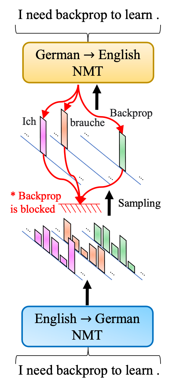
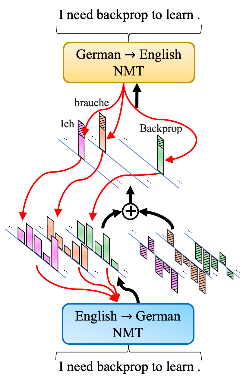
      (a) Previous BT                       (b) BT with CRT

Figure 1: Examples of English-to-German-to-English monolingual process of (a) previous BT and (b) BT with our proposed CRT. Given the English sentence, ’I need backprop to learn.’, they infer the German sentence, ’Ich brauche Backprop, um zu lemen.’ (only the first three words are illustrated for brevity). The solid black lines are forward propagations, and the thin red lines are backward propagations. While the sampling operation blocks the gradient flow in the previous works (a), the gradient flow detours to the inference model (English-to-German) in (b).

In this paper, we propose a new algorithm that handles the above challenges so that the two NMT models in the BT framework can be trained by end-to-end backpropagation, as in VAE. To overcome the non-differentiable issue, we propose a categorical reparameterization trick (CRT). By adding a conjugate part to the estimated categorical distribution, the CRT outputs an differentiable sentence, skipping the non-differentiable sampling process. Therefore, the end-to-end backpropagation finally updates the inference model to directly minimize with respect to the final objective function. The comparison of the previous BT works and the BT with our CRT is illustrated in Fig. 1. Additionally, we study the advantages of the CRT compared to the Gumbel-softmax trick (Jang et al., 2017), which is a popular reparameterization method for categorical distribution. In addition, in order to regularize the latent sentence to be realistic, we use the output distribution of the pre-trained language model (Bengio et al., 2003; Paszke et al., 2019) as the prior distribution of the latent sentence. Finally, we propose several regularization techniques that are advantageous to this unique framework.

In our experiments, we first analyze the benefits of our proposed method and regularizations with an ablation study on a custom low-resource dataset from the WMT18 translation task (Bojar et al., 2018). Then, we show that our proposed method improves the BLEU scores (Papineni et al., 2002) by around 0.29 and 0.80 on English-German and English-Turkish benchmark datasets, respectively. Based on these quantitative results, we demonstrate the advantage of end-to-end learning in the BT method and the importance of the CRT in this framework.

2 Related Works

2.1 Back-translation (BT) for NMT

Using a monolingual corpus for the NMT task often improves translation performance because it can give additional information for language understanding. As a practical method, the BT method was proposed (Sennrich et al., 2015) and the main idea is augmenting the bilingual corpus with synthetic pairs. While training ST-NMT, a pre-trained TS-NMT model, which was pre-trained by only bilingual corpus, translates target-language monolingual sentences into source-language synthetic sentences. Then, the synthetic source-language sentences and the corresponding target-language monolingual input sentences become synthetic pairs which are used as additional bilingual sentence pairs.

Several decoding methods have been used for the synthetic sentence’s translation, such as greedy, beam search, stochastic sampling, filtered sampling (Cheng, 2019; He et al., 2016; Imamura et al., 2018; Edunov et al., 2018; Fadaee & Monz, 2018; Graça et al., 2019; Caswell et al., 2019; Wu et al., 2019). Among them, stochastic sampling or filtered sampling demonstrated promising performances. However, it needs the condition that the pre-trained model should have been trained in enough iterations with enough size of the bilingual corpus. Otherwise, the noise can cause undesirable translation results because the initial translation quality of the pre-trained model is not acceptable. Therefore, selecting a translation method is still an undetermined topic.

To improve the translation performance, the iterative back-translation (IBT) method conducts a single BT training process multiple times (Hoang et al., 2018). In the IBT method, both ST-NMT and TS-NMT models are trained, given both languages of monolingual corpora. The synthetic sentences are iteratively updated by the improved NMT models, and the quality of the synthetic pairs improves gradually. As a result, it outperforms the single BT methods significantly. The IBT method can be divided into three ways according to the update timings of synthetic sentences: offline IBT, online IBT, and semi-online IBT. Offline IBT updates the whole synthetic sentences after the models converge within a single BT process. Different from the offline IBT, online IBT updates a mini-batch of the synthetic sentences in every iteration. Semi-online IBT follows the same strategy as the online IBT, but it sometimes loads previous synthetic sentences from memory given a pre-defined probability (Han et al., 2021). In this paper, we follow the online IBT method or the semi-online IBT for each translation task.

Following the IBT method, a probabilistic framework was proposed considering the translated synthetic sentence as an inferred latent variable that is the aligned representation of the monolingual input sentence (Cotterell & Kreutzer, 2018; Zhang et al., 2018). As described in Section 1, this BT framework is naturally connected to VAE based on the auto-encoding framework. For the sake of the reader’s understanding, we repeatedly summarize important terminologies in this paper. In the case of the source-to-target-to-source (STS) process, the ST-NMT model plays the role of the inference model (approximated posterior estimator), and it infers a latent sentence in the target-language domain given a source-language monolingual sentence. The TS-NMT model plays the role of the generation model (likelihood estimator), and it generates the input source-language monolingual sentence. In the target-to-source-to-target (TST) process, ST-NMT and TS-NMT play opposite roles.

However, it is still challenging to train the NMT models in the BT framework because of the non-differentiable latent sentences in the inference stage. Previous works proposed expectation-maximization algorithm (Cotterell & Kreutzer, 2018; Zhang et al., 2018) or backpropagation with ignoring the update of the inference model (Xu et al., 2020). In these cases, the inference model loses the learning signal that would have been propagated from the generation model. Therefore, it might find a worse local optimum because of the inefficient optimization. In this paper, we propose a new trick that reparameterizes the inferred latent sentence so that the end-to-end backpropagation can be feasible as in conventional VAE.

2.2 Binary Reparameterization Trick

Learning discrete representations in neural networks has several advantages. First, it is proper to represent discrete variables such as characters or words in natural language. Second, it can be efficiently implemented at the hardware-level. Lower memory cost and faster matrix multiplication than those of continuous representations are attractive properties (Hubara et al., 2016; Rastegari et al., 2016).

However, because of the non-differentiable property of the discrete representation, a gradient could not be backward propagated through it. To overcome this challenge, the straight-through estimator (STE) was proposed (Bengio et al., 2013), which estimates the gradient for discretizing operations (e.g., sampling or argmax operations) as 1 if the output is 1, otherwise it estimates 0. Although STE imposes a bias on the lower layer’s gradient estimation, it is empirically demonstrated as an effective gradient estimator in the training of existing binary neural networks (Hubara et al., 2016; Rastegari et al., 2016). The STE estimator can be implemented with automatic differentiation tools such as Pytorch (Raiko et al., 2014; Paszke et al., 2019). With a smart reparameterization technique, it outputs a differentiable binary representation as follows.

$$s \sim Bern(p),\quad s\in\{0,1\},$$ (1)

$$c =s(1-p)+(1-s)(-p),$$ (2)

$$z =p+\text{detach}(c),$$ (3)

where $p$ is a normalized probability of the binary variable. $Bern(p)$ and $s$ are the Bernoulli distribution with a parameter $p$ and its random variable. $\text{detach}(c)$ is the operation that detaches its input, $c$, from the gradient computation graph in backward propagation stage. As a result, the final output, $z$, is a binary variable, $z\in\{0,1\}$, and it can flow the gradient through the first term, $p$. As a variant of STE, it is easy to implement and work with other network architectures (Rim et al., 2021).

3 Proposed Method: E2E-BT

In this section, we propose a new method, E2E-BT, for end-to-end training of the BT framework like VAE. In Section 3.1, we propose the new reparameterization trick to handle the non-differentiable property of the latent sentence. In Section 3.2, we derive the objective functions for training in the BT framework with our proposed reparameterization trick. Also, we propose to use the language model’s output distribution as an appropriate prior distribution of the latent sentence. Finally, in Section 3.3, we propose several regularization techniques that can be advantageous to the BT framework.

3.1 Categorical Reparameterization Trick (CRT)

The distribution of a sentence is based on a sequence of categorical distributions of words, and a sampled sentence from the distribution is non-differentiable. To make backpropagation feasible through the sentence, we propose CRT, a reparameterization trick for categorical distribution, that is inspired by the binary reparameterization trick as in Section 2.2. Because we handle the categorical distribution (also called as Multinoulli distribution), the Bernoulli distribution in Eq. 1 is replaced by the Multinoulli distribution with the probability $\boldsymbol{p}$ computed by the inference model. Then, a one-hot vector for one word, $\boldsymbol{s}\in\{0,1\}^{|V|}$ s.t. $\sum_{i=1}^{|V|}{\boldsymbol{s}_{i}}=1$, is sampled from the distribution where $V$ is the vocabulary set. The CRT process can be formulated as follows.

$$\boldsymbol{s} \sim Mult(\boldsymbol{p}),$$ (4)

$$\boldsymbol{c} =\boldsymbol{s}\odot(\boldsymbol{1}-\boldsymbol{p})+(\boldsymbol{1}-\boldsymbol{s})\odot(-\boldsymbol{p}),$$ (5)

$$\boldsymbol{z} =\boldsymbol{p}+\text{detach}(\boldsymbol{c}),$$ (6)

where $\odot$ is the element-wise multiplication. $Mult(\boldsymbol{p})$ is the Multinoulli distribution given the normalized probability vector. Based on $\boldsymbol{p}$, we compute the non-differentiable conjugate part, $\boldsymbol{c}$, that is determined by the sample, $\boldsymbol{s}$. Finally, it outputs a one-hot encoded vector $\boldsymbol{z}$ which consists of the deterministic part $\boldsymbol{p}$ and the stochastic part $\boldsymbol{c}$ which is detached from the computation graph. Therefore, backpropagation can flow gradient into the lower layers through $\boldsymbol{p}$. Fig. 1 illustrates the whole process of this trick in the BT framework.

3.1.1 Comparison between Gumbel-Softmax Trick (GST)

One might ask “What is the benefit of the CRT compared to the Gumbel-softmax trick?” (Jang et al., 2017), which is a popular reparameterization trick for categorical distribution. We believe that the CRT has two benefits compared to the GST.

• Fast Computation: the CRT has less computation cost than the GST.

• Controllable Gradient: the CRT can control the amount of backward propagated gradient, while the GST cannot.

First, the CRT is computationally less expensive because the GST operates the softmax function twice while the CRT operates it only once. The two softmax operations of the GST are as follows: one for computing the normalized word probability vector to match the scale with Gumbel distribution’s sample and the other for the final output (Jang et al., 2017). The softmax function is expensive especially when the number of classes is large which is the case for natural language processing tasks. In experiments, we measured the spending times on reparameterization processes of the GST in Pytorch library’s implementation (Paszke et al., 2019) and our CRT. The vocabulary size, sentence length, and mini-batch size were set to 30000, 50, and 60, respectively. In the result, while the GST spent 3.35 seconds, our CRT spent 0.98 seconds, which is more than three times faster.

More importantly, the CRT can reparameterize any word, while the GST reparameterizes only the word with the maximum probability. That is, our CRT can select any word to reparameterize instead of using stochastic sampling methods or argmax in Eq. (4). This is a crucial property, especially when the BT framework is implemented with the Transformer architecture (Vaswani et al., 2017) which is the standard model in various natural language processing tasks these days. The inference process of the BT framework follows free-running where Transformer estimates every word’s probability multiple times until the translation finishes. At every step, Transformer estimates the distributions of all words, including the previous output words. Thus, it is possible that the distribution of the previous word changes due to the stochasticity of the model such as dropout (srivastava2014dropout). That is, the maximally probable words in the final estimation might not be the same as the word sampled previously (See Fig. 2). This situation may be even more frequent if we use stochastic sampling as the word sampling method. When there is discrepancy between the previous sampled words and the final words, it disturbs the gradient direction of the inference model in the wrong direction because the generation model computes and backpropagates the gradient based on the final output words, while the inference model receives the gradient assuming that it is computed based on the different words.

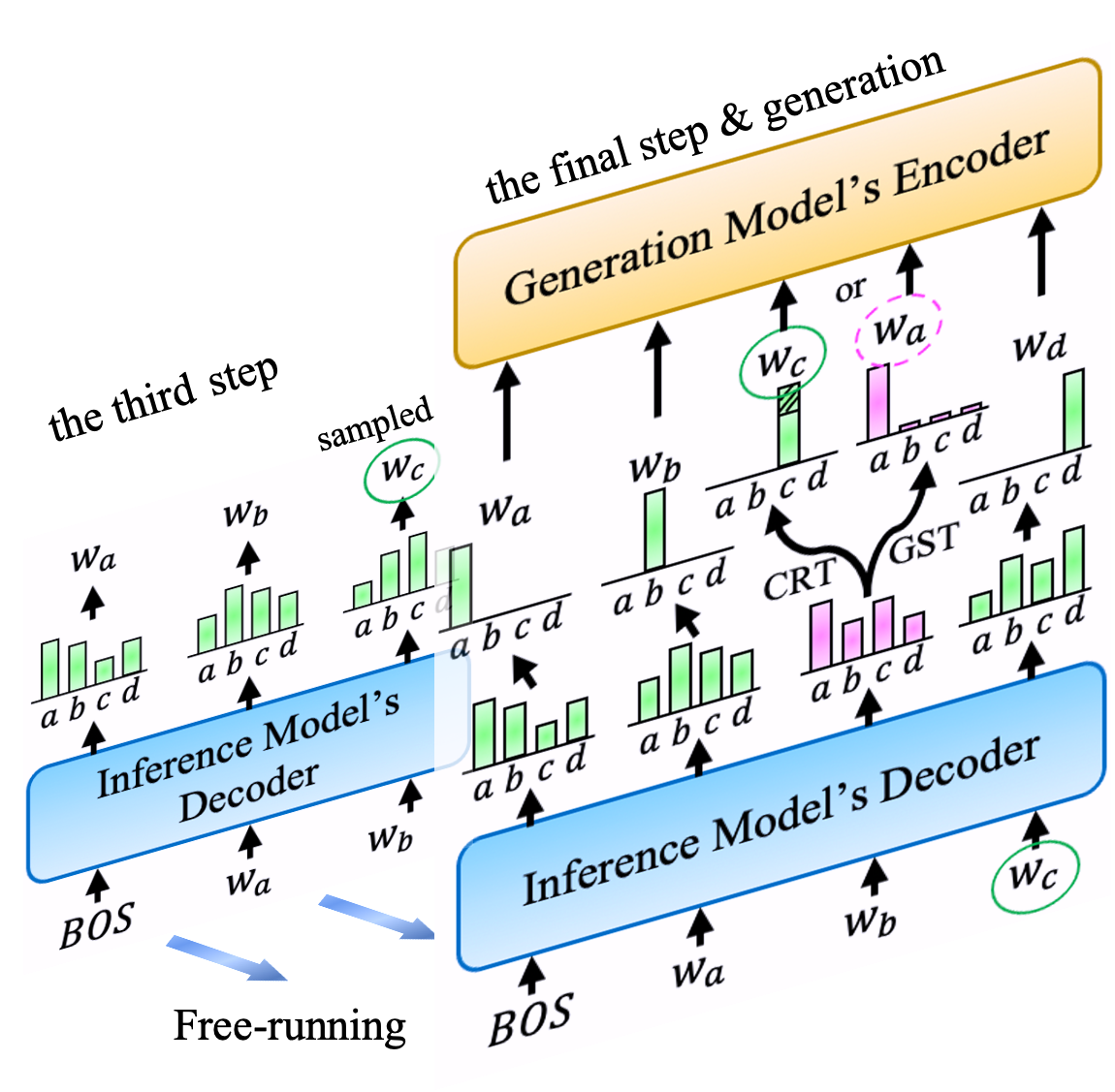
Figure 2: Example of the BT process with different reparameterization tricks, our CRT or the GST, where the third word’s distribution at the third step (green) changed at the next step (pink). Our CRT can output the previous word, $w_{c}$, while the GST only outputs the maximally probable word, $w_{a}$, as the final output.

Fig. 2 gives an example with the vocabulary set, $\{w_{a},w_{b},w_{c},w_{d}\}$. At the third step of the free-running inference, the word, $w_{c}$, is sampled from the third distribution (marked in green). However, in the next final step, the newly computed third distribution (marked in pink) is different from the previous one. Then, the GST samples a different word that has the maximum probability ($w_{a}$ in the figure) as the final output of the latent sentence, which is not the original conditional word, $w_{c}$, of the final estimation. Now, the generation model computes and backpropagates gradient through the last word, $w_{d}$, and it enforces the inference model to update its probability of $w_{d}$ given the final latent sentence, (BOS, $w_{a}$, $w_{b}$, $w_{a}$), as conditional words. However, the inference model will update assuming that the conditional words were (BOS, $w_{a}$, $w_{b}$, $w_{c}$). Contrary to the GST, our CRT can avoid this problem by just selecting $w_{c}$ instead of the maximum word.

In addition, our CRT can control simply the amount of backpropagated gradient. In practice, the backpropagation might lead the inference model to learn undesirable degenerating solutions, such as copying for the easiest reconstruction. Therefore, the scale of the gradient needs to be adjusted to find a desirable solution. The CRT can adjust the backward propagated gradient by just multiplying the word probability with a coefficient in the reparameterization process. Specifically, we multiply the coefficient, $\lambda$, to the probability term, $\boldsymbol{p}$, in Eqs. 5 and 6 as follows.

$$\boldsymbol{c} =\boldsymbol{s}\odot(\boldsymbol{1}-\lambda\boldsymbol{p})+(\boldsymbol{1}-\boldsymbol{s})\odot(-\lambda\boldsymbol{p}),$$ (7)

$$\boldsymbol{z} =\lambda\boldsymbol{p}+\text{detach}(\boldsymbol{c}).$$ (8)

Then, $\lambda$ plays a role of the additional learning rate only for the inference model. We can set two coefficients, $\lambda_{x}$ and $\lambda_{y}$, for two languages, respectively, if they need different controls. In the GST, this trick is hard to implement.

As a result of those disadvantages, we empirically show that the GST is not an appropriate reparameterization method in the BT framework, as shown in Table 1.

3.2 End-to-End Training in the BT Framework

In this section, we describe our objective functions for our end-to-end BT training. The final objective function can be decomposed into two terms with two types of processes: bilingual and monolingual processes. The first objective term for the bilingual process is cross-entropy as follows:

$$\mathcal{J}_{ST}(\theta) =-\sum_{(x^{b},y^{b})\in D^{b}}\log{p_{\theta}(y^{b}|x^{b})},$$ (9)

where $x^{b}$ and $y^{b}$ are a source-language and its paired target-language sentences in the bilingual corpus, $D^{b}$, respectively. $\theta$ is the parameter of the ST-NMT model. Likewise, the objective function for the TS-NMT model, $\mathcal{J}_{TS}(\phi)$, is computed in the same way by switching the source and target sentences and replacing the $\theta$ with the TS-NMT model’s parameter, $\phi$.

On the other hand, the objective function for the monolingual process is defined by the negative log likelihood of the monolingual sentence as follows:

$$\mathcal{J}_{TST} =-\sum_{y^{m}\in D^{y}}\log{p(y^{m})},$$ (10)

where $y^{m}$ is a target-language monolingual sentence in its monolingual corpus, $D^{y}$. The formulations are provided only for the TST process, but the STS process is simply symmetric to the TST process.

As usual, $\log{p(y^{m})}$ in Eq. 10 can be marginalized with latent sentences as follows:

$$\log{p(y^{m})} =\log{\sum_{\hat{x}\sim p(\hat{x})}p(y^{m}|\hat{x})p(\hat{x})},$$

where $\hat{x}$ is the inferred latent sentence that is the aligned representation of $y^{m}$ in the source language domain, and $p(\hat{x})$ is a prior distribution of $\hat{x}$. By introducing an approximated posterior distribution, $q(\hat{x}|y)$, which is easy to sample $\hat{x}$ given $y^{m}$, we can derive the evidence lower bound objective (ELBO) of the marginal probability, $\log{p(y^{m})}$, based on Jensen’s inequality as follows:

$$\log{p(y^{m})} \geq\sum_{\hat{x}\sim q(\hat{x}|y^{m})}q(\hat{x}|y^{m})\log{\frac{p(y^{m}|\hat{x})p(\hat{x})}{q(\hat{x}|y^{m})}},$$

$$\begin{split}&=\mathbb{E}_{\hat{x}\sim q(\hat{x}|y^{m})}[\log{p(y^{m}|\hat{x})}]\\ &\qquad-D_{KL}[q(\hat{x}|y^{m})\parallel p(\hat{x})],\end{split}$$

where $D_{KL}$ is Kullback-Liebler divergence (KL). In this TST process of the BT framework, the inference model, $q(\hat{x}|y^{m})$, is modeled by the TS-NMT model with parameter $\phi$. Also, the generation model, $p(y^{m}|\hat{x})$, is modeled by the ST-NMT with parameter $\theta$.

As we mentioned in the introduction section 1, the latent sentence, $\hat{x}$, should be a valid sentence in the source language domain. Therefore, we use the language model’s output distribution (Bengio et al., 2003; Paszke et al., 2019) as the prior distribution in the KL term, $p(\hat{x})$, instead of isotropic Gaussian in the conventional VAE. In practice, ELBO of the TST monolingual process can be formulated as follows:

$$\begin{split}\mathcal{J}^{ELBO}_{TST}(\phi,\theta)&=\sum_{y^{m}\in D^{y}}\mathbb{E}_{\hat{x}\sim q_{\phi}(\hat{x}|y^{m})}[\log{p_{\theta}(y^{m}|\hat{x})}]\\ &\quad-\alpha_{x}D_{KL}[q_{\phi}(\hat{x}|y^{m})\parallel p_{\psi_{x}}(\hat{x})],\end{split}$$ (11)

where $p_{\psi_{x}}(\hat{x})$ is the pre-trained and fixed source language model, and $\alpha_{x}$ is a hyperparameter to control the effect of the KL term in the final objective function. Importantly, to make backpropagation feasible through the latent sentence, we apply the CRT to the latent sentence, $\hat{x}$.

Finally, the total objective functions for $\theta$ and $\phi$ are as follows:

$$\mathcal{J}_{T}(\theta,\phi) =\mathcal{J}_{ST}(\theta)-\mathcal{J}^{ELBO}_{TST}(\phi,\theta),$$ (12)

$$\mathcal{J}_{S}(\phi,\theta) =\mathcal{J}_{TS}(\phi)-\mathcal{J}^{ELBO}_{STS}(\theta,\phi).$$ (13)

The parameters of the both translation models are updated by the two objective functions.

3.3 Regularization Techniques for BT

In this section, we propose additional regularization techniques that would improve performance of our proposed original approach in Section 3.2. Those regularizations are inspired by the peculiar characteristics of the BT framework, such as pairwise corpus utilization, shareable parameters, and stochasticity.

3.3.1 Freezing Evaluating Generation Model (FEG)

To maximize the utilization of pairwise corpus, our original approach in Section 3.2 first pre-train the parameters of both NMT models, $\theta$ and $\phi$, with the bilingual corpus. Therefore, in the BT framework, the generation model would enforce the inference model to infer desirable latent sentences from the beginning of the monolingual processes. However, this desirable enforcement could be faded as the training goes on. Therefore, we propose a novel regularization technique that can preserve this enforcement which is inspired by the target Q-network update technique in the deep Q-network algorithm (Mnih et al., 2013, 2015). We duplicate the generation model into two models, evaluating and learning, and freeze the parameter of the evaluating generation model for $k$ iterations. The evaluating generation model computes the loss that backpropagates to the inference model. On the other hand, the learning generation model computes the loss that is used to update its own parameters. The evaluating generation model’s parameters are updated every $k$-th iteration by copying it from the learning generation model, as in the deep Q-network algorithms. By doing this, the inference model can be trained with less faded desirable enforcement.

3.3.2 Sharing Embedding Parameters (SEP)

To improve the performance of our proposed method, we share the parameters between word embedding matrices of both NMT models. By doing this, not only reducing the number of parameters, but also we can expect the word embedding space to be regularized by both inference and generation models in iterations.

3.3.3 Annealing Stochasticity (AS)

Lastly, as argued in (Edunov et al., 2018), using stochastic sampling in the inference method gives more chances to find a better solution than the greedy method. However, adding more noise to the inference from the beginning of the training can cause the generation model to learn undesirable translation mapping, especially when the bilingual corpus is small. Therefore, we anneal the ratio of stochastic sampling during the training process as like the scheduled sampling approach in NMT (Bengio et al., 2015). That is, we infer the latent sentence by only the greedy method at the beginning and slowly increase the ratio of stochastic sampling as the training goes on.

4 Experiments and Results

Our experiments include an ablation study and benchmark experiments. The ablation study was conducted on a custom English-German dataset which is a small subset of WMT18 English-German dataset (Bojar et al., 2018). In the experiment, we analyze the advantages of our proposed methods individually in terms of tokenized BLEU score. After then, we evaluate our proposed method on large and small benchmark datasets, the English-German (En-De) and the English-Turkish (En-Tr) datasets from the WMT18 translation task. In these experiments, we demonstrate the advantages of our proposed method in terms of BLEU score compared to the baseline. The differences between the baseline and our BT method are the reparameterization, language model based prior distribution and regularization techniques described in Section 3.1.1 $\sim$ 3.3.

4.1 Ablation Study

As we described above, our ablation study was conducted on a small subset of the En-De dataset from the WMT18 translation task. After filtering out sentences longer than 50 words, the dataset contains 85K bilingual corpus and 464K monolingual corpus each for English and German. The total number of vocabulary (subwords) is 10,000. It was jointly used for both languages. We used ‘Newstest2017’ dataset as the validation dataset, which has 3,000 bilingual sentences.

For the NMT models, we used the Transformer model with only three encoder and decoder layers. The parameters of the NMT models were pre-trained by bilingual corpus only. For the language models used for the prior distribution estimator in Eq. (11), we adopted the Transformer-based language models (Paszke et al., 2019) which were pre-trained with bilingual and monolingual corpora for both languages respectively. Note that we did not use any other additional data to train the language models. We trained them with the same datasets that were used for the NMT’s pre-training and the main BT training.

For the optimization, we used the training strategy of fairseq toolkit (Ott et al., 2019). The optimizer was Adam (Kingma & Ba, 2014) with the learning rate of 0.001 and the mini-batch size was 60. In addition, the inverse root square scheduler was used for the learning rate schedule. This optimization setting was used for NMTs pre-training, language models pre-training, and main BT training.

For the main BT training, we followed the online IBT method (in Section 2.1). It is also important how mini-batch consists of bilingual and monolingual sentences. Following the empirical results of (Fadaee & Monz, 2018), each mini-batch consisted of 12 bilingual sentences and 48 monolingual sentences. About the configuration of our BT method, we set 0.01 for both $\lambda_{x}$ and $\lambda_{y}$. We set 0.0025 for both coefficients of the KL terms, $\alpha_{x}$ and $\alpha_{y}$. We individually applied the three regularization techniques described in Section 3.3. For FEG regularization, we set $k=75$ as the iteration number to freeze the evaluating generation model. For AS regularization, we linearly increased the ratio of stochastic sampling from 0 to 0.5 during 300K iterations.

Table 1: Ablation study results in terms of BLEU score. Models were trained on the custom En-De dataset, and validated with the ‘Newstest2017’. Then it was tested on ‘Newstest2018’. We used the beam search with a width of 5. In each evaluation, the left and right numbers of ‘$\mid$’ are En2De and De2En translation scores, respectively. We re-implemented the baseline models ‘Bilingual NMT (ours)’ and ‘Baseline BT (ours)’.

Model	Newstest 2017 (Validation)	Newstest 2018 (Test)
Bilingual NMT (ours)	10.53 $\mid$ 12.45	12.32 $\mid$ 14.19
Baseline BT (ours)	15.87 $\mid$ 18.87	19.97 $\mid$ 22.48
E2E BT w/ GST	2.05 $\mid$ 2.92	4.28 $\mid$ 5.46
E2E-BT	16.50 $\mid$ 19.67	20.91 $\mid$ 23.42
E2E-BT +FEG	16.36 $\mid$ 19.62	21.08 $\mid$ 23.36
E2E-BT +SEP	16.56 $\mid$ 20.28	20.96 $\mid$ 23.73
E2E-BT +AS	16.50 $\mid$ 20.04	20.80 $\mid$ 23.30

Table 2: Comparison on benchmark datasets, En-De and En-Tr, from the WMT18 translation task. ‘E2E-BT + Regs’ means our proposed BT method with additional regularizations, specifically FEG and AS. The scores of ‘Bilingual NMT@’ and ‘Baseline BT@’ are adapted from (Xu et al., 2020), and ‘Bilingual NMT (ours)’ and ‘Baseline BT (ours)’ are from our re-implementations. We used the beam search with a width of 5. In each evaluation of En-De ‘Newstest’, the left and right numbers of ‘$\mid$’ are En2De and De2En translation scores, respectively. It is the same order in the En-Tr evaluations (i.e., En2Tr $\mid$ Tr2En).

Model	En-De and De-En (Large Resource)				En-Tr and Tr-En (Small Resource)
	Newstest 2016	Newstest 2017	Newstest 2018	Avg.	Newstest 2017	Newstest 2018	Avg.
Bilingual NMT @	29.18 $\mid$ 31.95	23.46 $\mid$ 27.74	34.53 $\mid$ 34.59	30.24	11.17 $\mid$ 15.14	10.18 $\mid$ 15.95	13.11
Baseline BT @	29.99 $\mid$ 33.64	24.42 $\mid$ 29.13	35.60 $\mid$ 36.37	31.53	13.90 $\mid$ 17.18	11.84 $\mid$ 18.08	15.25
Bilingual NMT (ours)	31.12 $\mid$ 34.20	25.15 $\mid$ 30.19	37.05 $\mid$ 36.74	32.41	14.57 $\mid$ 15.08	13.60 $\mid$ 16.42	14.92
Baseline BT (ours)	32.20 $\mid$ 37.54	26.31 $\mid$ 32.50	38.39 $\mid$ 39.82	34.46	19.90 $\mid$ 21.05	17.66 $\mid$ 23.18	20.45
E2E-BT +Regs	32.09 $\mid$ 37.88	27.19 $\mid$ 32.76	39.08 $\mid$ 39.49	34.75	20.81 $\mid$ 21.82	18.47 $\mid$ 23.90	21.25

Table 1 presents the testing results of the ablation study on the ‘Newstest2017’ and ‘Newstest2018’ datasets, which were the validation and test datasets, respectively. Compared to ‘Bilingual NMT (ours)’, all of the BT methods significantly improves the performance, except the ‘E2E BT w/ GST’, which has the same training configuration as our ‘E2E-BT’ except that it uses GST instead of CRT as the reparameterization method. As we discussed in Section 3.1.1, we believe that the differences between CRT and GST were crucial in the BT training process and determined the end-to-end backpropagation’s feasibility. Compared to the ‘Baseline BT (ours)’, our proposed BT method without regularization techniques, ‘E2E-BT’, significantly improves the performance. In addition, when we add regularization techniques like ’+FEG’, ’+SEP’, or ’+AS’, they improve further.

4.2 Experiments on Benchmark Datasets

To validate the advantages of E2E-BT on benchmark datasets, we used En-De and En-Tr datasets from the WMT18 translation task after filtering out sentences that are longer than 50 words. The En-De dataset has 4.9M bilingual corpus, and the monolingual corpora for both languages have 4.8M sentences, respectively. The En-Tr dataset has 193K bilingual corpus, and the monolingual corpora of both languages have 4.4M sentences, respectively. We categorized the En-De and En-Tr datasets into large and small resource datasets, respectively. Like the ablation study, we used joined vocabulary sets with the sizes of 32,000 and 10,000 for En-De and En-Tr, respectively. For the validation sets, we used ‘Newstest2015 En-De’ (2,100 sentences) and ‘Newstest2016 En-Tr’ (3,000 sentences) for each language pair.

Unlike the ablation study, we used a bigger Transformer architecture that has 6 encoder and decoder layers. We used the same pre-training strategies as in the ablation study above. The configurations of the main BT training for the benchmark experiments are as follows. For the large En-De dataset, we set 0.01 for both $\lambda_{x}$ and $\lambda_{y}$, and 0.00005 for both coefficients of the KL terms, $\alpha_{x}$ and $\alpha_{y}$. Also, we used AS with the same configuration as the ablation study. For the small En-Tr dataset, we set 0.01 for both $\lambda$ terms, and 0.0001 for both coefficients of the KL terms. Like the En-De experiment, we used the AS regularization with the same configurations, except the FEG regularization with $k=100$. Additionally, we used the online IBT method for the En-Tr dataset, but for the En-De dataset, we set the semi-online method with a 75% probability of loading from memory after hyperparameter searching.

Table 2 presents the testing results on benchmark datasets. For a reliable evaluation, we tested on several ‘Newstest’ datasets. We reinforced the baseline models with our re-implementations ‘Bilingual NMT (ours)’ and ‘Baseline BT (ours)’, while the results of ‘Bilingual NMT @’ and ‘Baseline BT @’ are from the previous work (Xu et al., 2020). Our re-implementations show significantly better performances than the previous baseline models, because we used advanced training techniques from the fairseq toolkit such as learning rate schedule and checkpoint ensemble. In addition, we used a larger monolingual corpora for En-Tr experiment (4.4M vs. 0.8M). More importantly, ‘E2E-BT +Regs’, which is our proposed end-to-end training method, shows better performances in almost every evaluation. On average, our method improves 0.29 and 0.80 BLEU scores compared to the stronger baseline on En-De and En-Tr, respectively.

The results confirm that the end-to-end training fashion can find a better local optimum, as we discussed in earlier sections. Also, for the feasibility of end-to-end training, CRT could be an effective reparameterization method. Especially, our method shows a bigger improvement on the smaller dataset, which we think is because the end-to-end approach could correct unstable optimization caused by training on a small dataset.

5 Conclusion

In this paper, we proposed a categorical reparameterization trick that makes the translated sentences differentiable. Based on the trick, backpropagation became feasible through the sentences, and we used this trick to train both translation models in the end-to-end learning fashion for back-translation. To train the models together in back-translation, we developed the evidence lower bound objective, which could train the translation models in the semi-supervised learning fashion. In addition, we proposed several regularization techniques that are practically advantageous. Finally, our experimental results demonstrated that our proposed method is beneficial to learn better translation models which outperform the baselines.

References

- Bahdanau et al. (2014) Bahdanau, D., Cho, K., and Bengio, Y. Neural machine translation by jointly learning to align and translate. arXiv preprint arXiv:1409.0473, 2014.
- Bengio et al. (2015) Bengio, S., Vinyals, O., Jaitly, N., and Shazeer, N. Scheduled sampling for sequence prediction with recurrent neural networks. Advances in neural information processing systems, 28, 2015.
- Bengio et al. (2003) Bengio, Y., Ducharme, R., Vincent, P., and Jauvin, C. A neural probabilistic language model. Journal of machine learning research, 3(Feb):1137–1155, 2003.
- Bengio et al. (2013) Bengio, Y., Léonard, N., and Courville, A. Estimating or propagating gradients through stochastic neurons for conditional computation. arXiv preprint arXiv:1308.3432, 2013.
- Bojar et al. (2018) Bojar, O., Federmann, C., Fishel, M., Graham, Y., Haddow, B., Koehn, P., and Monz, C. Findings of the 2018 conference on machine translation (wmt18). In Proceedings of the Third Conference on Machine Translation, volume 2, pp. 272–307, 2018.
- Caswell et al. (2019) Caswell, I., Chelba, C., and Grangier, D. Tagged back-translation. arXiv preprint arXiv:1906.06442, 2019.
- Cheng (2019) Cheng, Y. Semi-supervised learning for neural machine translation. In Joint training for neural machine translation, pp. 25–40. Springer, 2019.
- Cotterell & Kreutzer (2018) Cotterell, R. and Kreutzer, J. Explaining and generalizing back-translation through wake-sleep. arXiv preprint arXiv:1806.04402, 2018.
- Currey et al. (2017) Currey, A., Miceli-Barone, A. V., and Heafield, K. Copied monolingual data improves low-resource neural machine translation. In Proceedings of the Second Conference on Machine Translation, pp. 148–156, 2017.
- Domhan & Hieber (2017) Domhan, T. and Hieber, F. Using target-side monolingual data for neural machine translation through multi-task learning. In Proceedings of the 2017 Conference on Empirical Methods in Natural Language Processing, pp. 1500–1505, 2017.
- Edunov et al. (2018) Edunov, S., Ott, M., Auli, M., and Grangier, D. Understanding back-translation at scale. arXiv preprint arXiv:1808.09381, 2018.
- Fadaee & Monz (2018) Fadaee, M. and Monz, C. Back-translation sampling by targeting difficult words in neural machine translation. arXiv preprint arXiv:1808.09006, 2018.
- Goodfellow et al. (2016) Goodfellow, I., Bengio, Y., and Courville, A. Deep Learning. MIT Press, 2016. http://www.deeplearningbook.org.
- Graça et al. (2019) Graça, M., Kim, Y., Schamper, J., Khadivi, S., and Ney, H. Generalizing back-translation in neural machine translation. arXiv preprint arXiv:1906.07286, 2019.
- Gulcehre et al. (2015) Gulcehre, C., Firat, O., Xu, K., Cho, K., Barrault, L., Lin, H.-C., Bougares, F., Schwenk, H., and Bengio, Y. On using monolingual corpora in neural machine translation. arXiv preprint arXiv:1503.03535, 2015.
- Guo et al. (2021) Guo, Y., Zhu, H., Lin, Z., Chen, B., Lou, J.-G., and Zhang, D. Revisiting iterative back-translation from the perspective of compositional generalization. In Proceedings of the AAAI Conference on Artificial Intelligence, volume 35, pp. 7601–7609, 2021.
- Hahn & Choi (2019) Hahn, S. and Choi, H. Disentangling latent factors of variational auto-encoder with whitening. In International Conference on Artificial Neural Networks, pp. 590–603. Springer, 2019.
- Han et al. (2021) Han, J. M., Babuschkin, I., Edwards, H., Neelakantan, A., Xu, T., Polu, S., Ray, A., Shyam, P., Ramesh, A., Radford, A., et al. Unsupervised neural machine translation with generative language models only. arXiv preprint arXiv:2110.05448, 2021.
- He et al. (2016) He, D., Xia, Y., Qin, T., Wang, L., Yu, N., Liu, T.-Y., and Ma, W.-Y. Dual learning for machine translation. Advances in neural information processing systems, 29:820–828, 2016.
- Higgins et al. (2017) Higgins, I., Matthey, L., Pal, A., Burgess, C. P., Glorot, X., Botvinick, M. M., Mohamed, S., and Lerchner, A. Beta-vae: Learning basic visual concepts with a constrained variational framework. In ICLR, 2017.
- Hoang et al. (2018) Hoang, V. C. D., Koehn, P., Haffari, G., and Cohn, T. Iterative back-translation for neural machine translation. In Proceedings of the 2nd Workshop on Neural Machine Translation and Generation, pp. 18–24, 2018.
- Hubara et al. (2016) Hubara, I., Courbariaux, M., Soudry, D., El-Yaniv, R., and Bengio, Y. Binarized neural networks. Advances in neural information processing systems, 29, 2016.
- Imamura et al. (2018) Imamura, K., Fujita, A., and Sumita, E. Enhancement of encoder and attention using target monolingual corpora in neural machine translation. In Proceedings of the 2nd Workshop on Neural Machine Translation and Generation, pp. 55–63, 2018.
- Jang et al. (2017) Jang, E., Gu, S., and Poole, B. Categorical reparametrization with gumble-softmax. In International Conference on Learning Representations (ICLR 2017). OpenReview. net, 2017.
- Kim & Mnih (2018) Kim, H. and Mnih, A. Disentangling by factorising. In International Conference on Machine Learning, pp. 2649–2658. PMLR, 2018.
- Kingma & Ba (2014) Kingma, D. P. and Ba, J. Adam: A method for stochastic optimization. arXiv preprint arXiv:1412.6980, 2014.
- Kingma & Welling (2013) Kingma, D. P. and Welling, M. Auto-encoding variational bayes. arXiv preprint arXiv:1312.6114, 2013.
- Mnih et al. (2013) Mnih, V., Kavukcuoglu, K., Silver, D., Graves, A., Antonoglou, I., Wierstra, D., and Riedmiller, M. Playing atari with deep reinforcement learning. arXiv preprint arXiv:1312.5602, 2013.
- Mnih et al. (2015) Mnih, V., Kavukcuoglu, K., Silver, D., Rusu, A. A., Veness, J., Bellemare, M. G., Graves, A., Riedmiller, M., Fidjeland, A. K., Ostrovski, G., et al. Human-level control through deep reinforcement learning. nature, 518(7540):529–533, 2015.
- Ott et al. (2019) Ott, M., Edunov, S., Baevski, A., Fan, A., Gross, S., Ng, N., Grangier, D., and Auli, M. fairseq: A fast, extensible toolkit for sequence modeling. In Proceedings of NAACL-HLT 2019: Demonstrations, 2019.
- Papineni et al. (2002) Papineni, K., Roukos, S., Ward, T., and Zhu, W.-J. Bleu: a method for automatic evaluation of machine translation. In Proceedings of the 40th annual meeting of the Association for Computational Linguistics, pp. 311–318, 2002.
- Paszke et al. (2019) Paszke, A., Gross, S., Massa, F., Lerer, A., Bradbury, J., Chanan, G., Killeen, T., Lin, Z., Gimelshein, N., Antiga, L., Desmaison, A., Kopf, A., Yang, E., DeVito, Z., Raison, M., Tejani, A., Chilamkurthy, S., Steiner, B., Fang, L., Bai, J., and Chintala, S. Pytorch: An imperative style, high-performance deep learning library. In Wallach, H., Larochelle, H., Beygelzimer, A., d'Alché-Buc, F., Fox, E., and Garnett, R. (eds.), Advances in Neural Information Processing Systems 32, pp. 8024–8035. Curran Associates, Inc., 2019.
- Raiko et al. (2014) Raiko, T., Berglund, M., Alain, G., and Dinh, L. Techniques for learning binary stochastic feedforward neural networks. arXiv preprint arXiv:1406.2989, 2014.
- Rastegari et al. (2016) Rastegari, M., Ordonez, V., Redmon, J., and Farhadi, A. Xnor-net: Imagenet classification using binary convolutional neural networks. In European conference on computer vision, pp. 525–542. Springer, 2016.
- Rim et al. (2021) Rim, D. N., Jang, I., and Choi, H. Deep neural networks and end-to-end learning for audio compression. arXiv preprint arXiv:2105.11681, 2021.
- Sennrich et al. (2015) Sennrich, R., Haddow, B., and Birch, A. Improving neural machine translation models with monolingual data. arXiv preprint arXiv:1511.06709, 2015.
- Skorokhodov et al. (2018) Skorokhodov, I., Rykachevskiy, A., Emelyanenko, D., Slotin, S., and Ponkratov, A. Semi-supervised neural machine translation with language models. In Proceedings of the AMTA 2018 workshop on technologies for MT of low resource languages (LoResMT 2018), pp. 37–44, 2018.
- Vaswani et al. (2017) Vaswani, A., Shazeer, N., Parmar, N., Uszkoreit, J., Jones, L., Gomez, A. N., Kaiser, Ł., and Polosukhin, I. Attention is all you need. In Advances in neural information processing systems, pp. 5998–6008, 2017.
- Wu et al. (2019) Wu, L., Wang, Y., Xia, Y., Qin, T., Lai, J., and Liu, T.-Y. Exploiting monolingual data at scale for neural machine translation. In Proceedings of the 2019 Conference on Empirical Methods in Natural Language Processing and the 9th International Joint Conference on Natural Language Processing (EMNLP-IJCNLP), pp. 4207–4216, 2019.
- Xu et al. (2020) Xu, W., Niu, X., and Carpuat, M. Dual reconstruction: a unifying objective for semi-supervised neural machine translation. arXiv preprint arXiv:2010.03412, 2020.
- Zhang & Zong (2016) Zhang, J. and Zong, C. Exploiting source-side monolingual data in neural machine translation. In Proceedings of the 2016 Conference on Empirical Methods in Natural Language Processing, pp. 1535–1545, 2016.
- Zhang et al. (2018) Zhang, Z., Liu, S., Li, M., Zhou, M., and Chen, E. Joint training for neural machine translation models with monolingual data. In Thirty-Second AAAI Conference on Artificial Intelligence, 2018.