Two continuous (4, 5) pairs of explicit 9-stage Runge–Kutta methods

Abstract

An $11$-dimensional family of embedded $(4,5)$ pairs of explicit $9$-stage Runge–Kutta methods with an interpolant of order $5$ is derived. Two optimized for efficiency pairs are presented. embedded pair of Runge–Kutta methods, continuous formula, interpolant

1 Introduction

Runge–Kutta methods (see, e.g., (Butcher, 2008, sec. 23 and ch. 3), (Hairer et al., 2008, ch. II), (Ascher & Petzold, 1998, ch. 4), (Iserles, 2009, ch. 3)) are widely and successfully used to solve Ordinary Differential Equations (ODEs) numerically for over a century (Butcher & Wanner, 1996). Being applied to a system ${\rm d}\mkern 0.25mu{\boldsymbol{x}}/{\rm d}\mkern 0.25mut={\boldsymbol{f}}(t,\,{\boldsymbol{x}})$, in order to propagate by the step size $h$ and update the position, ${\boldsymbol{x}}(t)\mapsto{\boldsymbol{x}}(t+h)$, an $s$-stage explicit Runge-Kutta method (which is determined by the coefficients $a_{\mkern 1.0mui\mkern-1.0muj}$, weights $b_{\mkern-1.0muj}$, and nodes $c_{\mkern 0.5mui}$) would compute intermediate vectors ${\boldsymbol{F}}_{\mkern-1.0mu1}$, ${\boldsymbol{X}}_{\mkern-1.0mu2}$, ${\boldsymbol{F}}_{\mkern-1.0mu2}$, ${\boldsymbol{X}}_{\mkern-1.0mu3}$, …, ${\boldsymbol{X}}_{\mkern-1.0mus}$, ${\boldsymbol{F}}_{\mkern-3.0mus}$, and then ${\boldsymbol{x}}(t+h)$:

$${\boldsymbol{X}}_{\mkern-1.0mui}={\boldsymbol{x}}(t)+h\!\sum_{j=1}^{i-1}a_{\mkern 1.0mui\mkern-1.0muj}\mkern 2.0mu{\boldsymbol{F}}_{\mkern-3.5muj},\qquad{\boldsymbol{F}}_{\mkern-1.5mui}={\boldsymbol{f}}\bigl{(}t+c_{\mkern 0.5mui}\mkern 1.0muh,\mkern 2.0mu{\boldsymbol{X}}_{\mkern-1.0mui}\bigr{)},\qquad{\boldsymbol{x}}(t+h)={\boldsymbol{x}}(t)+h\!\sum_{j=1}^{s}b_{\mkern-1.25muj}\mkern 2.0mu{\boldsymbol{F}}_{\mkern-3.5muj}$$

In the limit $h\to 0$ all the vectors ${\boldsymbol{F}}_{\mkern-1.5mui}$, where $1\leq i\leq s$, are the same, so it is natural and will be assumed that $\sum_{\mkern-1.0muj=1}^{\mkern 0.5mui-1}a_{\mkern 1.0mui\mkern-1.0muj}=c_{\mkern 0.5mui}$. For $i=1$ the sum over $\mkern-1.0muj$ is empty, so $c_{1}=0$, ${\boldsymbol{X}}_{\mkern-1.0mu1}={\boldsymbol{x}}(t)$, and ${\boldsymbol{F}}_{\mkern-1.0mu1}=\smash{{\boldsymbol{f}}\bigl{(}t,\mkern 1.0mu{\boldsymbol{x}}(t)\bigr{)}}$.

To obtain an accurate solution with less effort, various adaptive step size strategies were developed (see, e.g., (Butcher, 2008, secs. 271 and 33), (Hairer et al., 2008, sec. II.4), (Ascher & Petzold, 1998, sec. 4.5), (Iserles, 2009, ch. 6)). Typically a system of ODEs is solved in two different ways, and the step size is chosen so that the two solutions are sufficiently close. A computationally efficient procedure is to have two Runge–Kutta methods with different weights, but the same nodes and coefficients. The vectors ${\boldsymbol{F}}_{1}$, ${\boldsymbol{F}}_{2}$, …, ${\boldsymbol{F}}_{\mkern-3.0mus}$ are computed only once, and then are used in both methods, the latter are said to form an embedded pair. Two well known examples of such pairs are (Fehlberg, 1969, tab. III), (Fehlberg, 1970, tab. 1) and (Dormand & Prince, 1980, tab. 2).

There is no $5$-stage explicit Runge–Kutta ${5}^{\textrm{th}}$ order method (Butcher, 1964). The Fehlberg pair has $6$ stages. The Dormand–Prince pair uses $7$ stages, but has the so-called First Same As Last (FSAL) property (Fehlberg, 1969, p. 17), (Dormand & Prince, 1978): the vector ${\boldsymbol{F}}_{\mkern-1.0mu1}$ at the current step is equal to the already computed ${\boldsymbol{F}}_{\mkern-2.0muu}$ at the stage $1<u\leq s$ of the previous step. An FSAL method requires $(s-1)$ evaluations of the r.h.s. function ${\boldsymbol{f}}$ per step, with the exception of the $1^{\textrm{st}}$ step.

 order           $t$  $\gamma(t)$  $\sigma(t)$           ${\boldsymbol{\Phi}}(t)$ $1^{\textrm{st}}$ $1$ $1$ ${\boldsymbol{1}}\vphantom{|_{|}^{|}}$ $2^{\textrm{nd}}$ $2$ $1$ ${\boldsymbol{c}}\vphantom{|_{|}^{|}}$ $3^{\textrm{rd}}$ $3$ $2$ ${\boldsymbol{c}}^{2}$ $\downarrow$ $6$ $1$ ${\boldsymbol{A}}\mkern 1.0mu{\boldsymbol{c}}={\boldsymbol{c}}^{2}\mkern-1.0mu/2+{\boldsymbol{q}}_{1}\vphantom{|_{|}^{|}}$ ${4}^{\textrm{th}}$ $4$ $6$ ${\boldsymbol{c}}^{3}$ $\downarrow$ $8$ $1$ $({\boldsymbol{A}}\mkern 1.0mu{\boldsymbol{c}})\mkern 1.0mu{\boldsymbol{c}}={\boldsymbol{c}}^{3}\mkern-1.0mu/2+c_{2}\mkern 1.0mu{\boldsymbol{q}}_{1}$ $12$ $2$ ${\boldsymbol{A}}\mkern 1.0mu{\boldsymbol{c}}^{2}={\boldsymbol{c}}^{3}\mkern-1.0mu/3+{\boldsymbol{q}}_{2}$ $24$ $1$ ${\boldsymbol{A}}^{2}\mkern 1.0mu{\boldsymbol{c}}={\boldsymbol{A}}\mkern 1.0mu{\boldsymbol{c}}^{2}/2+{\boldsymbol{A}}\mkern 1.0mu{\boldsymbol{q}}_{1}\vphantom{|_{|}^{|}}$ ${5}^{\textrm{th}}$ $5$ $24$ ${\boldsymbol{c}}^{4}$ $\downarrow$ $10$ $2$ $({\boldsymbol{A}}\mkern 1.0mu{\boldsymbol{c}})\,{\boldsymbol{c}}^{2}={\boldsymbol{c}}^{4}\mkern-1.0mu/2+c_{2}^{2}\mkern 1.0mu{\boldsymbol{q}}_{1}$ $15$ $2$ $({\boldsymbol{A}}\mkern 1.0mu{\boldsymbol{c}}^{2})\mkern 1.0mu{\boldsymbol{c}}={\boldsymbol{c}}^{4}\mkern-1.0mu/3+{\boldsymbol{q}}_{2}\mkern 1.0mu{\boldsymbol{c}}$ $30$ $1$ $({\boldsymbol{A}}^{2}\mkern 1.0mu{\boldsymbol{c}})\mkern 1.0mu{\boldsymbol{c}}=({\boldsymbol{A}}\mkern 1.0mu{\boldsymbol{c}}^{2})\,{\boldsymbol{c}}/2+({\boldsymbol{A}}\mkern 1.0mu{\boldsymbol{q}}_{1}\mkern-1.5mu)\mkern 1.0mu{\boldsymbol{c}}$ $20$ $2$ $({\boldsymbol{A}}\mkern 1.0mu{\boldsymbol{c}})^{2}={\boldsymbol{c}}^{4}\mkern-1.0mu/4+c_{2}^{2}\mkern 1.0mu{\boldsymbol{q}}_{1}/2$ $20$ $6$ ${\boldsymbol{A}}\mkern 1.0mu{\boldsymbol{c}}^{3}={\boldsymbol{c}}^{4}\mkern-1.0mu/4+{\boldsymbol{q}}_{3}$ $40$ $1$ ${\boldsymbol{A}}\bigl{(}\mkern-1.0mu({\boldsymbol{A}}\mkern 1.0mu{\boldsymbol{c}})\mkern 1.0mu{\boldsymbol{c}}\mkern-0.5mu\bigr{)}={\boldsymbol{A}}\mkern 1.0mu{\boldsymbol{c}}^{3}\mkern-1.0mu/2+c_{2}\mkern 1.0mu{\boldsymbol{A}}\mkern 1.0mu{\boldsymbol{q}}_{1}$ $60$ $2$ ${\boldsymbol{A}}^{2}\mkern 1.0mu{\boldsymbol{c}}^{2}={\boldsymbol{A}}\mkern 1.0mu{\boldsymbol{c}}^{3}\mkern-1.0mu/3+{\boldsymbol{A}}\mkern 1.0mu{\boldsymbol{q}}_{2}$ $120$ $1$ ${\boldsymbol{A}}^{3}\mkern 1.0mu{\boldsymbol{c}}={\boldsymbol{A}}^{2}\mkern 1.0mu{\boldsymbol{c}}^{2}/2+{\boldsymbol{A}}^{2}\mkern 1.0mu{\boldsymbol{q}}_{1}$

Table 1: Order conditions ${\boldsymbol{b}}\mkern 1.0mu{\boldsymbol{\Phi}}(t)=1/\gamma(t)$ for rooted trees $t$ with up to $5$ vertices. It is assumed that $({\boldsymbol{A}}\mkern 1.0mu{\boldsymbol{c}})_{\mkern 0.5mui}=c_{\mkern 0.5mui}^{2}/2$ for all $i\neq 2$.

Continuous formulas or interpolants (see, e.g., (Horn, 1983), Sarafyan (1984), (Butcher, 2008, sec. 272), (Hairer et al., 2008, sec. II.6)) provide an inexpensive (i.e., with only a few if any additional evaluations of the r.h.s.) way to estimate the solution at anywhere within the integration interval. Without altering the strategy of step size choice, this can be used in applications that require values of the solution ${\boldsymbol{x}}(t)$ at specific points $t_{1}$, $t_{2}$, … (dense output) or the place (time $t$ and/or position ${\boldsymbol{x}}(t)$) where the solution crosses a hypersurface $\smash{g\bigl{(}t,\mkern 1.0mu{\boldsymbol{x}}(t)\bigr{)}=0}$ (event location). The continuous approximation to the solution in the interval $[\mkern 1.0mut,\,t+h\mkern 1.0mu]$ is typically of the form

$${\boldsymbol{x}}(t+\theta h)={\boldsymbol{x}}(t)+h\!\sum_{j=1}^{s}\beta_{\mkern-0.25muj}(\theta)\mkern 2.0mu{\boldsymbol{F}}_{\mkern-3.5muj}$$

where the interpolant functions $\beta_{\mkern-0.25muj}(\theta)=\sum_{k}\beta_{k\mkern-1.0muj}\theta^{k}$ are polynomials. For the approximation over several step intervals to be continuously differentiable a method should have the FSAL property, with the following conditions on the behavior of the row vector ${\boldsymbol{\beta}}(\theta)=\bigl{[}\beta_{\mkern-0.25muj}(\theta)\bigr{]}$ at $\theta=0$ and $\theta=1$:

$$c_{1} =0, {\boldsymbol{a}}_{1*} ={\boldsymbol{0}}={\boldsymbol{\beta}}(0), {\boldsymbol{X}}_{\mkern-1.0mu1} ={\boldsymbol{x}}(t), {\boldsymbol{F}}_{\mkern-1.0mu1} ={\boldsymbol{f}}\bigl{(}t,\,{\boldsymbol{x}}(t)\bigr{)}, \frac{{\rm d}\beta_{\mkern-0.25muj}(\theta)}{{\rm d}\theta}\Bigr{|}_{\theta=0} =\left\{\begin{array}[]{ll}1,&j=1\\ 0,&j\neq 1\end{array}\right.$$

$$c_{u} =1, {\boldsymbol{a}}_{u*} ={\boldsymbol{b}}={\boldsymbol{\beta}}(1), {\boldsymbol{X}}_{\mkern-1.0muu} ={\boldsymbol{x}}(t+h), {\boldsymbol{F}}_{\mkern-2.0muu} ={\boldsymbol{f}}\bigl{(}t+h,\,{\boldsymbol{x}}(t+h)\bigr{)}, \frac{{\rm d}\beta_{\mkern-0.25muj}(\theta)}{{\rm d}\theta}\Bigr{|}_{\theta=1} =\left\{\begin{array}[]{ll}1,&j=u\\ 0,&j\neq u\end{array}\right.$$

Here ${\boldsymbol{a}}_{i*}=\bigl{[}a_{\mkern 1.0mui\mkern-1.0muj}\bigr{]}$ and ${\boldsymbol{b}}=\bigl{[}b_{\mkern-1.25muj}\bigr{]}$ are the row vectors of coefficients and weights, respectively. Below all interpolants are assumed to be continuously differentiable.

The product of column vectors ${\boldsymbol{x}}\mkern 2.0mu{\boldsymbol{y}}$ is to be understood element-wise: $({\boldsymbol{x}}\mkern 2.0mu{\boldsymbol{y}})_{i}=x_{i}\mkern 1.0muy_{i}$. Let ${\boldsymbol{1}}$ be the $s$-dimensional column vector with all components being equal to $1$; ${\boldsymbol{c}}=\bigl{[}c_{i}\bigr{]}$ be the nodes vector; and ${\boldsymbol{A}}=\bigl{[}a_{\mkern 1.0mui\mkern-1.0muj}\bigr{]}$ be the $s\times s$ matrix with $a_{\mkern 1.0mui\mkern-1.0muj}$ as its matrix element in the $i^{\mkern 1.0mu\textrm{th}}$ row and $j^{\mkern 1.0mu\textrm{th}}$ column (for an explicit method $a_{\mkern 1.0mui\mkern-1.0muj}=0$ if $i\leq j$). Let ${\boldsymbol{q}}_{n}={\boldsymbol{A}}\mkern 1.0mu{\boldsymbol{c}}^{n}-\frac{1}{n+1}\mkern 1.0mu{\boldsymbol{c}}^{n+1}$. The condition $\sum_{j}a_{\mkern 1.0mui\mkern-1.0muj}=c_{i}$, ${\boldsymbol{A}}{\boldsymbol{1}}={\boldsymbol{c}}$, or ${\boldsymbol{q}}_{0}={\boldsymbol{0}}$ is assumed. The following quantities will be used for the estimation of the local error:

$$T_{p}^{2}({\boldsymbol{x}},\theta)=\sum_{\mathclap{\text{rooted~{}trees~{}}t\text{~{}of~{}order~{}}p}}\tau^{2}(t,\mkern 2.0mu{\boldsymbol{x}},\theta),\qquad\tau(t,\mkern 2.0mu{\boldsymbol{x}},\theta)=\frac{1}{\sigma(t)}\biggl{(}{\boldsymbol{x}}\mkern 1.5mu{\boldsymbol{\Phi}}(t)-\frac{\theta^{p}}{\gamma(t)}\biggr{)}$$

Here $\sigma(t)$ is the order of the symmetry group of the tree $t$ (see, e.g., (Butcher, 2008, p. 140)). Whenever the argument ${\boldsymbol{x}}$ or $\theta$ is omitted, its value is meant to be equal to ${\boldsymbol{\beta}}(\theta)$ and $1$, respectively. Note that ${\boldsymbol{\beta}}(1)={\boldsymbol{b}}$. An interpolant of order $p$ should satisfy the conditions $\tau(t,\theta)\equiv 0$ for all rooted trees $t$ with up to $p$ vertices. For $p=5$, with the assumption that the intermediate positions ${\boldsymbol{X}}_{\mkern-1.0mui}$ are at least $2^{\textrm{nd}}$ order accurate for all $i>2$, these conditions are listed in Table 1, see also (Butcher, 2008, sec. 31), (Hairer et al., 2008, sec. II.2), (Dormand & Prince, 1980, tab. 1).

There are certain properties one would expect from a practical Runge–Kutta method (see, e.g., a list in (Verner, 1978, p. 785)). The natural or desirable behavior of the interpolant function $\beta_{\mkern-0.25muj}(\theta)$, where $1\leq j\leq s$, is that it has a notably positive slope around $\theta\approx c_{\mkern-1.25muj}$, while it is hardly changing anywhere else. Deviations from this behavior can be divided into two categories: non-positivity, when an interpolant function’s derivative is negative; and non-locality, when an interpolant function has substantial slope (positive or negative) far from the position of the corresponding node.

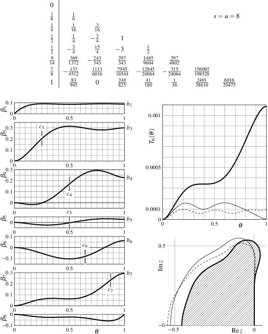
Figure 1: The continuous $(4,5)$ pair (Owren & Zennaro, 1992, fig. 3): the Butcher tableau (upper panel), the weights vector ${\boldsymbol{b}}$ repeats the last row of ${\boldsymbol{A}}$ and is not shown; the interpolant functions $\beta_{\mkern-0.25muj}(\theta)$, with $j=1$, $3$, $4$, …, $8$ (the panels on the left, the function $\beta_{\mkern 1.5mu2}(\theta)\equiv 0$ is not shown); the local error $T_{6}(\theta)$ (middle right panel); and the region of absolute stability (lower right panel). (The thin dashed and solid lines correspond to the pairs on Figure 3 and Figure 5, respectively. The three regions of absolute stability are scaled for equal cost, i.e., the regions where $\bigl{|}\mkern 1.0muR\bigl{(}\mkern-1.0mu(s-1)\mkern 1.0muz\bigr{)}\bigr{|}\leq 1$ are depicted, here $R(z)$ is the stability function and $s$ is the number of stages.)

An explicit Runge–Kutta method with continuously differentiable interpolant of order $5$ has at least $8$ stages (Owren & Zennaro, 1991, sec. 3.3). Such methods were completely classified in (Verner & Zennaro, 1995). In (Owren & Zennaro, 1992) a $5$-dimensional family of continuous $(4,5)$ pairs of $8$-stage Runge-Kutta methods was constructed, and an optimized for efficiency (Owren & Zennaro, 1992, fig. 3) pair was suggested, which is also shown in Figure 1. All the pairs in this $5$-dimensional family satisfy $2c_{3}=c_{4}=c_{5}$. This is an indication that the family lacks sufficient flexibility or is stressed by numerous imposed conditions. Looking at the interpolant functions in Figure 1, $\beta_{4}(\theta)$ goes down for $\theta>0.8$, $\beta_{6}(\theta)$ goes down for $\theta<0.5$, and both $\beta_{7}(\theta)$ and $\beta_{8}(\theta)$ express non-locality for $\theta<0.3$.

Any Runge–Kutta method could be equipped with an interpolant by adding, if needed, additional stages (Enright et al., 1986), (Verner, 1993). Several interpolants were constructed for the (Dormand & Prince, 1980, tab. 2) pair, see, e.g., (Shampine, 1986, p. 149) and (Calvo et al., 1990). With $u=7$ both interpolants use $s=9$ stages (see also (Owren & Zennaro, 1991, corollary 2.13)). The second interpolant has somewhat smaller local error, see (Calvo et al., 1990, fig. 1).

Increasing the number of stages (and thus the amount of computation per step) provides additional flexibility in choosing the nodes, coefficients, and weights, which may be exploited to construct viable pairs that produce an accurate solution in fewer steps. In (Sharp & Smart, 1993, sec. 3.1) and (Bogacki & Shampine, 1996) non-FSAL embedded $(4,5)$ pairs of $7$-stage Runge–Kutta methods were suggested. The objective in the construction of the latter pair was an improvement of the (Dormand & Prince, 1980, tab. 2) pair (see (Bogacki & Shampine, 1996, p. 19)). The pair was also equipped with an interpolant of order $5$. The minimal number of stages would be $9$, but in (Bogacki & Shampine, 1996) the suggested interpolant (with the local error, to the leading order, being a problem-independent function of the local error at the end of the step) is using $11$ stages.

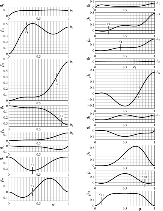
Figure 2: The interpolant functions $\beta_{\mkern-0.25muj}(\theta)$, with $j=1$, $3$, $4$, …, $9$ (Calvo et al., 1990) for the embedded $(4,5)$ pair (Dormand & Prince, 1980, tab. 2) (panels on the left, $s=9$, $u=7$) and functions $\beta_{\mkern-0.25muj}(\theta)$, with $j=1$, $3$, $4$, …, $11$, for the (Bogacki & Shampine, 1996) pair (panels on the right, $s=11$, $u=8$).

The interpolant (Calvo et al., 1990) for the (Dormand & Prince, 1980, tab. 2) pair and the interpolant for the (Bogacki & Shampine, 1996) pair are depicted in Figure 2. In the case of Dormand–Prince pair, $b_{5}<0$, plus the $1^{\textrm{st}}$ order condition $\sum_{j}\beta_{\mkern-0.25muj}(\theta)\equiv\theta$ is obtained through the cancellation of wiggles in $\beta_{3}$, $\beta_{8}$, $\beta_{9}$, and of slopes in $\beta_{4}$ and $\beta_{5}$ for $\theta>0.6$. In the case of Bogacki–Shampine pair, there is some non-locality in $\beta_{1}$, $\beta_{3}$, $\beta_{4}$, and $\beta_{6}$, which is compensated by $\beta_{9}$, $\beta_{10}$, and $\beta_{11}$. If an interpolant is obtained by adding stages to an already formed pair, the interpolant function for an added stage has a negative slope somewhere, as it should have zero values (and derivatives) at $\theta=0$ and $\theta=1$.

In this work embedded $(4,5)$ pairs are constructed, like the (Owren & Zennaro, 1992, fig. 3) pair, so that they have an interpolant right away, although not the minimal number of stages is used. The family of such pairs is constructed in Section 2. How the values of the free parameters are chosen is discussed in Section 3. The performance of built pairs is demonstrated in Section 4.

2 A family of continuous $\boldsymbol{(4,5)}$ pairs

There are two different ways to generate an embedded pair with an interpolant: to construct a pair with no interpolant, and then add one or several stages in order to build one; or to design both a pair and an interpolant at once. The latter approach is used here. As for continuous $(4,5)$ pairs $8$ stages do not provide enough flexibility (Owren & Zennaro, 1992), here $s=9$ stages are used. For the update of position, ${\boldsymbol{x}}(t)\mapsto{\boldsymbol{x}}(t+h)$, to be as accurate as possible, the FSAL stage is the last one: $u=9$.

To increase the similarity with collocation methods (see, e.g., (Hairer et al., 2008, p. 211), (Ascher & Petzold, 1998, sec. 4.7.1), (Iserles, 2009, sec. 3.4)), the Dominant Stage Order (DSO) (see, e.g., (Verner, 2010, eq. (5))) is chosen to be equal to $3$. This goes against the observation (Verner, 2010, p. 386) that most efficient for computation pairs of order $p$ have the DSO being equal to $(p-4)$ or $(p-3)$. Increasing the DSO makes order conditions more redundant, and may not reduce richness or flexibility of the set of pairs much.

The parameters of the $11$-dimensional family of continuous $(4,5)$ pairs described below are $c_{2}$, $c_{4}$, $c_{5}$, $c_{6}$, $c_{7}$, $c_{8}$, $a_{65}$, $a_{75}$, $a_{76}$, $a_{86}$, and $a_{87}$. Their values are arbitrary, except for some degenerate cases, e.g., $c_{5}=c_{4}$ for which the matrix ${\boldsymbol{A}}$ ends up being infinite. Other nodes $c_{1}$, $c_{3}$, $c_{9}$, and the first $8$ rows of ${\boldsymbol{A}}$ are expressed through the $11$ parameters as follows:

$$c_{1} =0,\qquad c_{3}=2c_{4}/3,\qquad c_{9}=1$$

$$h_{\mkern 1.0mui\mkern-1.0muj} =a_{\mkern 1.0mui\mkern-1.0muj}\mkern 1.0muc_{\mkern-1.25muj}(c_{\mkern-1.25muj}-c_{4})\mkern 3.0mu\bigg{/}\mkern 18.0mu\prod^{k\neq i}_{\mathclap{\mkern 12.0muk\in\{1,4,5,6,7,8\}}}\mkern 18.0mu(c_{i}-c_{k}),\qquad Y_{\mkern-1.0muj}=3-5c_{4}-5c_{\mkern-1.25muj}+10c_{4}c_{\mkern-1.25muj}$$

$$Z_{m} =12-15c_{4}-15c_{5}-15c_{m}+20c_{4}c_{5}+20c_{4}c_{m}+20c_{5}c_{m}-30c_{4}c_{5}c_{m}\quad\smash{\left.\vphantom{\rule{1.0pt}{42.0pt}}\right\}}\mkern 9.0mu\mbox{\small\smash{\begin{minipage}{57.81621pt} determines $a_{85}\vphantom{|_{|}^{|}}$\\ ensures $b_{9}=0\vphantom{|_{|}^{|}}$ \end{minipage}}}$$

$$\sum_{i\mkern-1.0muj\mkern 2.0mu\in\mathcal{S}}^{\phantom{i}}Y_{\mkern-1.0muj}\mkern 1.0muh_{\mkern 1.0mui\mkern-1.0muj}=\sum_{i\mkern-1.0muj\mkern 2.0mu\in\mathcal{S}}\sum_{k\mkern 0.5mul\mkern 1.0mu\in\mathcal{S}}(c_{i}-c_{k})(c_{\mkern-1.25muj}-c_{l})\mkern 1.0muZ_{21-i-k}\mkern 1.0muh_{\mkern 1.0mui\mkern-1.0muj}\mkern 1.0muh_{kl}$$

$$a_{\mkern 0.5mui\mkern 1.0mu4} =\frac{1}{c_{4}^{2}}\biggl{(}c_{i}^{2}(c_{i}-c_{4})-3\sum_{j=5}^{i-1}a_{\mkern 1.0mui\mkern-1.0muj}c_{j}(c_{j}-c_{3})\biggr{)},\qquad i\geq 4$$

$$a_{\mkern 0.5mui\mkern 1.0mu3} =\frac{1}{c_{3}^{2}}\biggl{(}c_{i}^{2}\bigl{(}c_{4}-{\textstyle\frac{2}{3}}c_{i}\bigr{)}+2\sum_{j=5}^{i-1}a_{\mkern 1.0mui\mkern-1.0muj}c_{j}(c_{j}-c_{4})\biggr{)},\qquad i\geq 4\hskip 24.0pt\raisebox{-13.0pt}{\smash{\begin{minipage}{10.84006pt}$\displaystyle\left.\vphantom{\rule{1.0pt}{60.0pt}}\right\}$\end{minipage}}}\mkern 9.0mu\mbox{\small\smash{\begin{minipage}{91.0598pt} $\phantom{.}$ \vskip 24.0ptensures $\vphantom{|_{|}}$\\ $\vphantom{.}$\quad${\boldsymbol{q}}_{0}={\boldsymbol{0}}\vphantom{|_{|}^{|}}$\\ $\vphantom{.}$\quad$({\boldsymbol{q}}_{1})_{i}=0\vphantom{|_{|}^{|}}$ for all $i\neq 2$\\ $\vphantom{.}$\quad$({\boldsymbol{A}}\mkern 1.0mu{\boldsymbol{q}}_{1}\mkern-1.5mu)_{i}=0\vphantom{|_{|}^{|}}$ for all $i\neq 3$ \\ $\vphantom{.}$\quad$({\boldsymbol{q}}_{2})_{i}=0\vphantom{|_{|}^{|}}$ for all $i\neq 2,3$ \end{minipage}}}$$

$$a_{\mkern 0.5mui\mkern 1.0mu2} =\left\{\begin{array}[]{ll}c_{3}^{2}/2c_{2},&\quad i=3\\ 0,&\quad i\neq 3\end{array}\right.$$

$$a_{\mkern 0.5mui\mkern 1.0mu1} =c_{i}-\sum_{j=2}^{i-1}a_{\mkern 1.0mui\mkern-1.0muj}\qquad\mbox{for all }i$$

where $\mathcal{S}=\{65,75,85,76,86,87\}$. In particular, $a_{41}=c_{4}/4$ and $a_{43}=3c_{4}/4$.

The vectors ${\boldsymbol{q}}_{2}$ and ${\boldsymbol{q}}_{2}\mkern 1.0mu{\boldsymbol{c}}$ are linear combinations of ${\boldsymbol{q}}_{1}$ and ${\boldsymbol{A}}\mkern 1.0mu{\boldsymbol{q}}_{1}$, also $({\boldsymbol{A}}\mkern 1.0mu{\boldsymbol{q}}_{1}\mkern-1.5mu)\mkern 1.0mu{\boldsymbol{c}}=c_{3}\mkern 1.5mu{\boldsymbol{A}}\mkern 1.0mu{\boldsymbol{q}}_{1}$. The four vectors ${\boldsymbol{q}}_{1}$, ${\boldsymbol{A}}\mkern 1.0mu{\boldsymbol{q}}_{1}$, ${\boldsymbol{A}}^{2}{\boldsymbol{q}}_{1}$, and ${\boldsymbol{q}}_{3}$ should be in the null space of the matrix ${\boldsymbol{B}}=\bigl{[}\beta_{k\mkern-1.0muj}\bigr{]}$, see Table 1. The interpolant matrix ${\boldsymbol{B}}$ is generated as

$${\boldsymbol{B}}=\left[\begin{array}[]{ccccccccc}\,1&\,0&\,0&\,0&\,0&\,0&\,0&\,0&\,0\\ 0&\frac{1}{2}&0&0&0&0&0&0&0\\ 0&0&\frac{1}{3}&0&0&0&0&0&0\\ 0&0&0&\frac{1}{4}&0&0&0&0&0\\ 0&0&0&0&\frac{1}{5}&0&0&0&0\end{array}\right]\underbrace{\left[\begin{array}[]{ccccccccc}{\boldsymbol{1}}&{\boldsymbol{c}}&{\boldsymbol{c}}^{2}&{\boldsymbol{c}}^{3}&{\boldsymbol{c}}^{4}&{\boldsymbol{q}}_{1}&{\boldsymbol{A}}\mkern 1.0mu{\boldsymbol{q}}_{1}&{\boldsymbol{A}}^{2}{\boldsymbol{q}}_{1}&{\boldsymbol{q}}_{3}\end{array}\right]}_{9\times 9\textrm{~{}matrix}}{{\vphantom{\big{|}}}^{-1}}$$ (7)

Here the last components of the four vectors ${\boldsymbol{q}}_{1}$, ${\boldsymbol{A}}\mkern 1.0mu{\boldsymbol{q}}_{1}$, ${\boldsymbol{A}}^{2}{\boldsymbol{q}}_{1}$, and ${\boldsymbol{q}}_{3}$ are set to $0$, which is compatible with the order conditions. The interpolant ${\boldsymbol{\beta}}(\theta)=\bigl{[}\,\theta~{}~{}~{}\theta^{2}~{}~{}~{}\theta^{3}~{}~{}~{}\theta^{4}~{}~{}~{}\theta^{5}\,\bigr{]}\,{\boldsymbol{B}}$ is continuously differentiable if

$$\left[\begin{array}[]{ccccc}1&\;0&\;0&\;0&\;0\\ 1&\;1&\;1&\;1&\;1\\ 1&\;2&\;3&\;4&\;5\end{array}\right]{\boldsymbol{B}}=\left[\begin{array}[]{ccccccccc}1&\;0&\;0&\;0&\;0&\;0&\;0&\;0&\;0\\ {\mkern 1.0mu}b{}_{1}&{\mkern 1.0mu}b_{2}{\mkern-1.0mu}&{\mkern 1.0mu}b_{3}{\mkern-1.0mu}&{\mkern 1.0mu}b_{4}{\mkern-1.0mu}&{\mkern 1.0mu}b_{5}{\mkern-1.0mu}&{\mkern 1.0mu}b_{6}{\mkern-1.0mu}&{\mkern 1.0mu}b_{7}{\mkern-1.0mu}&{\mkern 1.0mu}b_{8}{\mkern-1.0mu}&\;0\\ 0&\;0&\;0&\;0&\;0&\;0&\;0&\;0&\;1\end{array}\right]$$

The $1^{\textrm{st}}$ and $3^{\textrm{rd}}$ rows of this equation are satisfied automatically due to how the first and last rows of the $9\times 9$ matrix in eq. (7) look like. The $2^{\textrm{nd}}$ row is used to determine ${\boldsymbol{a}}_{9*}={\boldsymbol{b}}$. The interpolant functions $\beta_{2}(\theta)\equiv 0$ and $\beta_{3}(\theta)\equiv 0$ as $({\boldsymbol{q}}_{1})_{i}=0$ and $({\boldsymbol{A}}\mkern 1.0mu{\boldsymbol{q}}_{1}\mkern-1.5mu)_{i}=0$ for all $i\neq 2$ and $i\neq 3$, respectively.

The $5$-dimensional (could be parameterized by $c_{2}$, $c_{4}$, $c_{5}$, $c_{6}$, and $c_{7}$) family of $(5,6)$ pairs (see (Dormand et al., 1989, tab. 5), (Verner, 1991, tab. 2), (Sharp & Verner, 1994, tab. 4), (Verner, 2010, tab. 3)) is constructed in a similar fashion. It has $\textrm{DSO}=3$, $c_{8}=1$, and $a_{i2}=0$ for all $i\neq 3$. The $9\times 9$ matrix in the equation (7) is singular. With just $9$ stages, in order for the ${5}^{\textrm{th}}$ order interpolant to exist, the last $4$ columns of the matrix should be linearly dependent, which happens if $c_{4}=c_{5}$. Then the ${5}^{\textrm{th}}$ stage repeats the ${4}^{\textrm{th}}$ one, while some of the coefficients become infinite. To equip such an embedded $(5,6)$ pair with an interpolant of order $5$, one needs to add at least one more stage.

3 Choice of the degrees of freedom

A measure of the amount of non-positivity present in an interpolant is its total variation:

$$V\vphantom{|}_{0}^{1}({\boldsymbol{B}})=\sum_{j=1}^{s}\,\int\limits_{0}^{1}{\rm d}\theta\;\biggl{|}\frac{{\rm d}\beta_{\mkern-0.25muj}(\theta)}{{\rm d}\theta}\biggr{|}$$

As $\sum_{j}\beta_{\mkern-0.25muj}(\theta)\equiv\theta$, the minimal possible value of $V\vphantom{|}_{0}^{1}({\boldsymbol{B}})$ is equal to $1$. If the integration over $\theta$ is restricted to the region where $\beta_{\mkern-0.25muj}(\theta)$ has a negative slope: $N\vphantom{|}_{0}^{1}({\boldsymbol{B}})=\sum_{j}\int_{0}^{1}{\rm d}\theta\;\bigl{|}\beta^{\prime}_{\mkern-0.25muj}(\theta)\bigr{|}\,H\bigl{(}-\beta^{\prime}_{\mkern-0.25muj}(\theta)\bigr{)}$, then $V\vphantom{|}_{0}^{1}({\boldsymbol{B}})=1+2N\vphantom{|}_{0}^{1}({\boldsymbol{B}})$. Here $H$ is the Heaviside step function.

Figure 3: A continuous $(4,5)$ pair: the Butcher tableau and the region of absolute stability $\bigl{|}\mkern 1.0muR(z)\bigr{|}\leq 1$. The weights vector ${\boldsymbol{b}}$ repeats the last row of ${\boldsymbol{A}}$ and is not shown. The difference between the weights vectors of the ${4}^{\textrm{th}}$ and the ${5}^{\textrm{th}}$ order methods within the pair could be any linear combination of ${\boldsymbol{d}}_{1}$, ${\boldsymbol{d}}_{2}$, and ${\boldsymbol{d}}_{3}$. Regions of absolute stability of the (Dormand & Prince, 1980, tab. 2) pair (with $r_{7}=0$) and the (Bogacki & Shampine, 1996) pair (with $r_{7}=\frac{2421}{2464}$) are shown for comparison. The three regions of absolute stability shown on the small right panels are scaled for equal cost, i.e., the regions where $\bigl{|}\mkern 1.0muR\bigl{(}\mkern-1.0mu(s-1)\mkern 1.0muz\bigr{)}\bigr{|}\leq 1$ are depicted. For the (Dormand & Prince, 1980, tab. 2), (Bogacki & Shampine, 1996) pairs and the pair presented in this figure the number of stages $s$ is equal to $7$, $8$, $9$ on upper panel (just position is updated, ${\boldsymbol{x}}(t)\mapsto{\boldsymbol{x}}(t+h)$) and $9$, $11$, $9$ on lower panel (interpolant of order $5$ with $\max_{\,0\leq\theta\leq 1}T_{6}(\theta)\approx T_{6}$ is computed), respectively.

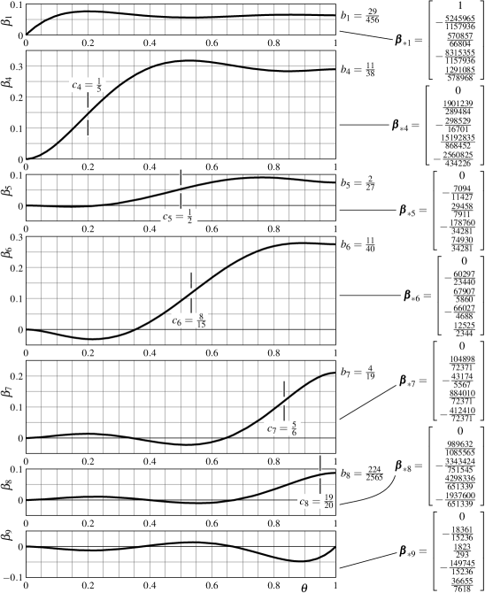
Figure 4: Columns of the matrix ${\boldsymbol{B}}$ and interpolant functions $\beta_{\mkern-0.25muj}(\theta)$, where $j=1$, $4$, $5$, …, $9$, for the pair shown in Figure 3.

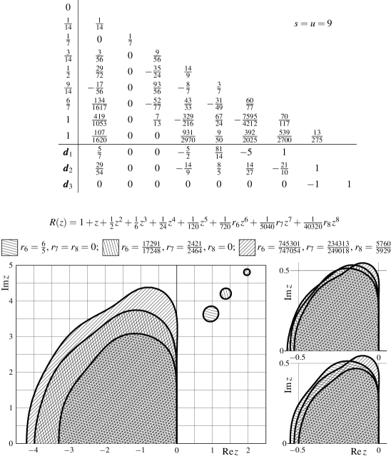
Figure 5: A continuous $(4,5)$ pair: the Butcher tableau and the region of absolute stability $\bigl{|}\mkern 1.0muR(z)\bigr{|}\leq 1$. The weights vector ${\boldsymbol{b}}$ repeats the last row of ${\boldsymbol{A}}$ and is not shown. The difference between the weights vectors of the ${4}^{\textrm{th}}$ and the ${5}^{\textrm{th}}$ order methods within the pair could be any linear combination of ${\boldsymbol{d}}_{1}$, ${\boldsymbol{d}}_{2}$, and ${\boldsymbol{d}}_{3}$. Regions of absolute stability of the (Dormand & Prince, 1980, tab. 2) pair (with $r_{7}=0$) and the (Bogacki & Shampine, 1996) pair (with $r_{7}=\frac{2421}{2464}$) are shown for comparison. The three regions of absolute stability shown on the small right panels are scaled for equal cost, i.e., the regions where $\bigl{|}\mkern 1.0muR\bigl{(}\mkern-1.0mu(s-1)\mkern 1.0muz\bigr{)}\bigr{|}\leq 1$ are depicted. For the (Dormand & Prince, 1980, tab. 2), (Bogacki & Shampine, 1996) pairs and the pair presented in this figure the number of stages $s$ is equal to $7$, $8$, $9$ on upper panel (just position is updated, ${\boldsymbol{x}}(t)\mapsto{\boldsymbol{x}}(t+h)$, or interpolant of order $4$, $4$, $5$ is computed) and $7$, $9$, $9$ on lower panel (low-cost interpolant of order $4$, $5$, $5$ is computed), respectively.

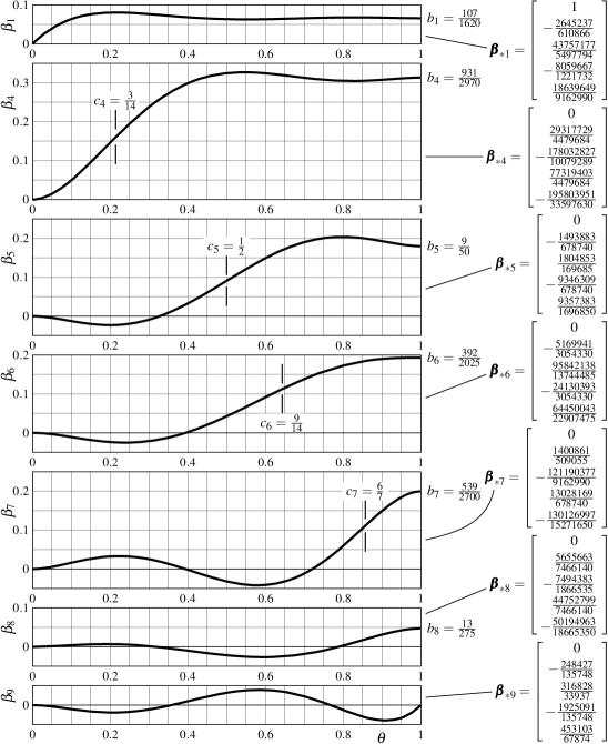
Figure 6: Columns of the matrix ${\boldsymbol{B}}$ and interpolant functions $\beta_{\mkern-0.25muj}(\theta)$, where $j=1$, $4$, $5$, …, $9$, for the pair shown in Figure 5.

The continuous $(4,5)$ pair shown in Figure 3 was obtained by minimizing the following function:

$$\max_{0\leq\theta\leq 1}T_{6}(\theta)+10^{-4}\mkern 2.0muV\vphantom{|}_{0}^{1}({\boldsymbol{B}})+10^{-7}\sum_{ij}\bigl{(}4|a_{\mkern 1.0mui\mkern-1.0muj}|^{2}+|a_{\mkern 1.0mui\mkern-1.0muj}|^{4}\bigr{)}$$

The term $\max_{0\leq\theta\leq 1}T_{6}(\theta)$ was motivated by the discussion in (Bogacki & Shampine, 1996, p. 24). In the resulted pair the local error $T_{6}$ is only slightly smaller than $\max_{\,0\leq\theta\leq 1}T_{6}(\theta)$, see Table 2. The term with $V\vphantom{|}_{0}^{1}({\boldsymbol{B}})$ makes the interpolant functions to wiggle less. For the pair to have rational coefficients, the values of the $11$ parameters obtained in the minimization were approximated by rational numbers.

The pair shown in Figure 5 was obtained by minimizing $T_{6}$ subject to the $T_{7}\leq 10T_{6}$ inequality constraint. (The (Dormand & Prince, 1980, tab. 2) and (Bogacki & Shampine, 1996, p. 20) pairs have the ratio $T_{7}/T_{6}$ close to $10$. For the latter pair this was a part of the design process.) A minor variation of the pair brings the local error $T_{6}$ to zero, see Table 4. The value of $\max_{0\leq\theta\leq 1}T_{6}(\theta)$ is much larger than $T_{6}$, see Table 2. This by itself is not necessarily problematic, as less accurate interpolant is connecting endpoints of the integration step that contain an error accumulated in many steps. With $(4,5)$ pairs it is not even uncommon to use interpolants of order $4$.

$$\begin{array}[]{r|lll|ll}&10^{5}\times T_{6}&10^{5}\times T_{7}&10^{5}\times\max_{\theta}T_{6}(\theta)&\max_{ij}|\mkern 1.0mua_{\mkern 1.0mui\mkern-1.0muj}\mkern 1.0mu|&\phantom{0}V\vphantom{|}_{0}^{1}({\boldsymbol{B}})\vphantom{|_{|}^{|}}\\ \hline\cr\mbox{Owren--Zennaro}&108.62...&154.05...&\phantom{00}108.62...&\phantom{0}3.75&1.6496...\vphantom{|_{|}^{|}}\\ \mbox{Dormand--Prince}&\phantom{0}39.908...&395.57...&\phantom{000}39.908...&11.595...&3.2490...\vphantom{|_{|}^{|}}\\ \mbox{Bogacki--Shampine}&{}\phantom{00}2.2169...&{}\phantom{0}21.260...&\phantom{0000}2.2169...&\phantom{0}1.1637...&3.3092...\vphantom{|_{|}^{|}}\\ \hline\cr\mbox{Figure~{}}\ref{pair1}&\phantom{00}9.2847...&\phantom{0}19.904...&\phantom{0000}9.7178...&\phantom{0}2.0803...&1.4857...\vphantom{|_{|}^{|}}\\ \mbox{Figure~{}}\ref{pair2}&\phantom{00}0.59809...&\phantom{00}5.9203...&\phantom{000}16.134...&\phantom{0}2.7916...&1.6424...\vphantom{|_{|}^{|}}\end{array}$$

Table 2: A comparison of five continuous $(4,5)$ pairs. The first three are from the literature: (Owren & Zennaro, 1992, fig. 3), (Dormand & Prince, 1980, tab. 2), and (Bogacki & Shampine, 1996).

$$\begin{array}[]{r|lll}&10^{5}\times T_{5}({\boldsymbol{x}})&10^{5}\times T_{6}({\boldsymbol{x}})&10^{5}\times T_{7}({\boldsymbol{x}})\vphantom{|_{|}^{|}}\\ \hline\cr\mbox{Dormand--Prince, }{\boldsymbol{x}}={\boldsymbol{b}}_{4^{\textrm{th}}\textrm{~{}order}}&118.29...&182.37...&414.05...\vphantom{|_{|}^{|}}\\ {\boldsymbol{x}}=\frac{1}{3}{\boldsymbol{b}}+\frac{2}{3}{\boldsymbol{b}}_{4^{\textrm{th}}\textrm{~{}order}}&\phantom{0}78.863...&118.66...&392.39...\vphantom{|_{|}^{|}}\\ \hline\cr\mbox{Bogacki--Shampine, }{\boldsymbol{x}}={\boldsymbol{b}}+{\boldsymbol{E}}&\phantom{0}10.595...&{}\phantom{0}12.204...&\phantom{0}24.114...\vphantom{|_{|}^{|}}\\ {\boldsymbol{x}}={\boldsymbol{B}}&\phantom{0}10.615...&\phantom{0}10.992...&\phantom{0}20.562...\vphantom{|_{|}^{|}}\\ \hline\cr\mbox{Figure~{}}\ref{pair1}\mbox{, }{\boldsymbol{x}}={\boldsymbol{b}}+\frac{1}{42}{\boldsymbol{d}}_{1}&\phantom{0}19.765...&\phantom{0}14.406...&\phantom{0}18.948...\vphantom{|_{|}^{|}}\\ {\boldsymbol{x}}={\boldsymbol{b}}-\frac{1}{323}{\boldsymbol{d}}_{2}&\phantom{0}19.465...&\phantom{0}29.174...&\phantom{0}33.473...\vphantom{|_{|}^{|}}\\ {\boldsymbol{x}}={\boldsymbol{b}}+\frac{1}{152}{\boldsymbol{d}}_{3}&\phantom{0}19.511...&\phantom{0}27.858...&\phantom{0}27.751...\vphantom{|_{|}^{|}}\\ \hline\cr\mbox{Figure~{}}\ref{pair2}\mbox{, }{\boldsymbol{x}}={\boldsymbol{b}}+\frac{1}{2430}{\boldsymbol{d}}_{1}&\phantom{00}0.99808...&\phantom{00}1.0189...&\phantom{00}6.0611...\vphantom{|_{|}^{|}}\\ {\boldsymbol{x}}={\boldsymbol{b}}+\frac{1}{2156}{\boldsymbol{d}}_{2}&\phantom{00}0.99189...&\phantom{00}1.4234...&\phantom{00}6.4042...\vphantom{|_{|}^{|}}\\ {\boldsymbol{x}}={\boldsymbol{b}}-\frac{1}{986}{\boldsymbol{d}}_{3}&\phantom{00}0.99041...&\phantom{00}1.3645...&\phantom{00}6.4662...\vphantom{|_{|}^{|}}\end{array}$$

Table 3: Local errors for the lower order methods of four embedded $(4,5)$ pairs. The second line of the (Dormand & Prince, 1980, tab. 2) entry is the modification suggested in (Shampine, 1986, p. 141). The notation ${\boldsymbol{E}}$ and ${\boldsymbol{B}}$ in the (Bogacki & Shampine, 1996) entry is taken from the

rksuite.f

code (Brankin et al., 1993).

$$\begin{array}[]{c|ccccccccc}0\vphantom{|_{|}^{|}}\\ \frac{1}{14}\vphantom{|_{|}^{|}}&\phantom{-}\frac{1}{14}&&&&&&&\mathclap{s=u=9}\\ \frac{1}{7}\vphantom{|_{|}^{|}}&\phantom{-}0&\phantom{-}\frac{1}{7}\\ \frac{3}{14}\vphantom{|_{|}^{|}}&\phantom{-}\frac{3}{56}&\phantom{-}0&\phantom{-}\frac{9}{56}\\ \frac{1}{2}\vphantom{|_{|}^{|}}&\phantom{-}\frac{29}{72}&\phantom{-}0&-\frac{35}{24}&\phantom{-}\frac{14}{9}\\ \frac{9}{14}\vphantom{|_{|}^{|}}&-\frac{17}{56}&\phantom{-}0&\phantom{-}\frac{93}{56}&-\frac{8}{7}&\phantom{-}\frac{3}{7}\\ \frac{6}{7}\vphantom{|_{|}^{|}}&\phantom{-}\frac{199}{1372}&\phantom{-}0&-\frac{195}{196}&\phantom{-}\frac{1259}{784}&-\frac{3855}{5488}&\phantom{-}\frac{45}{56}\\ 1\vphantom{|_{|}^{|}}&\phantom{-}\frac{4903}{25596}&\phantom{-}0&\phantom{-}\frac{4487}{2844}&-\frac{255101}{102384}&\phantom{-}\frac{33847}{11376}&-\frac{94325}{51192}&\phantom{-}\frac{3773}{6399}\\ 1\vphantom{|_{|}^{|}}&\phantom{-}\frac{16}{243}&\phantom{-}0&\phantom{-}0&\phantom{-}\frac{16807}{53460}&\phantom{-}\frac{53}{300}&\phantom{-}\frac{2401}{12150}&\phantom{-}\frac{2401}{12150}&\phantom{-}\frac{79}{1650}\\ \end{array}$$

Table 4: The Butcher tableau of the embedded $(4,6)$ pair with FSAL property. The weights vector ${\boldsymbol{b}}$, which produces the ${6}^{\textrm{th}}$ order update, repeats the last row of ${\boldsymbol{A}}$ and is not shown. The $9\times 9$ matrix in eq. (7) is non-singular, and no weights vector other than ${\boldsymbol{b}}$ would give a method of order $5$. The ${5}^{\textrm{th}}$ order interpolant is constructed as in eq. (7). The differences ${\boldsymbol{d}}_{1,2,3}$ between the weights vectors of the ${4}^{\textrm{th}}$ and the ${6}^{\textrm{th}}$ order methods, that could be used for error control, are the same as in Figure 5.

4 Numerical tests

The performance of the pairs constructed in the previous section is demonstrated on test problems A3, D5, and E2 from (Hull et al., 1972) in Figure 7; and on new suggested test problems U1, U2, and U4 in Figure 8. The error, that is the difference between the exact and numerical solutions, was computed only at the ends of integration steps. The adaptive step size scheme $h\leftarrow 0.9\mkern 1.0muh\mkern 1.5mu(\mbox{ATOL}/E)^{1/5}$ was used. (The starting step size $h_{0}=10^{-3}$ was swiftly corrected by the adaptive step size control.) Here ATOL is the absolute error tolerance, and $E$ is the $l^{2}$-norm of the difference vector between the two solutions within a pair. The steps with $E>\mbox{ATOL}$ were rejected, but they were still contributing to the number of the r.h.s. evaluations. For the pairs with multiple difference vectors between the weights of the higher and lower order methods (i.e., the (Bogacki & Shampine, 1996) pair and the pairs in Figures 3 and 5, see Table 3), the difference vectors that use smaller number of stages were tried first. Once a step was rejected, no further difference vectors were tried. The size of the next step, whether the previous step was rejected or not, was chosen according to the maximal value of $E$ between the tried vectors.

The pairs with higher order $6$ performed better on test problems A3 and D5. On other problems their performance was similar to the (Bogacki & Shampine, 1996) pair. The (Dormand & Prince, 1980, tab. 2) pair performed well on problem A3, while on problems E2, U2, and U4 it performed the worst. The pair shown in Figure 3 performed the worst on problems A3 and D5. The pair from Figure 5 seems to be at least as efficient as the (Bogacki & Shampine, 1996) pair. Note that the efficiency curves in Figures 7 and 8 show the cost of obtaining the numerical solution without computing interpolants. In case of the (Bogacki & Shampine, 1996) pair, no additional stages are needed to use the interpolant of order $4$ (Bogacki, 1990). One or three additional r.h.s. evaluations per step are needed to compute less and more accurate interpolant of order $5$, respectively (Bogacki & Shampine, 1996, p. 24), which corresponds to the increase of the cost by factors $8/7$ and $10/7$.

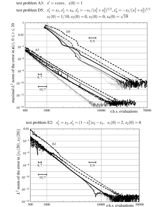
Figure 7: Efficiency curves for problems A3 (Hull et al., 1972, p. 617), D5 (Hull et al., 1972, p. 620), and E2 (Hull et al., 1972, p. 621): the (Dormand & Prince, 1980, tab. 2) pair (dash-dotted curve), the (Bogacki & Shampine, 1996) pair (dotted curve), the pair in Figure 3 (dashed curve), the pair in Figure 5 (solid curve), the $(4,6)$ pair in Table 4 (thin solid curve), and the (Verner, 2010, tab. 3) par (thin dotted curve).

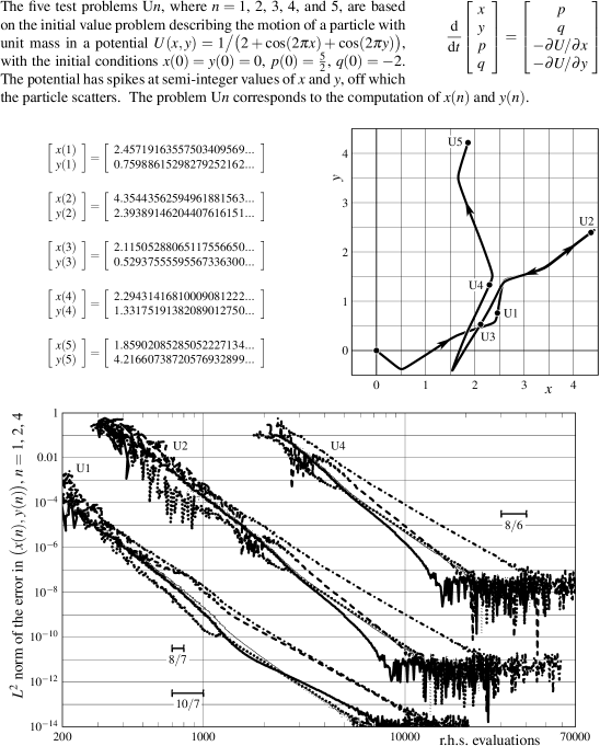
Figure 8: The test problems U$n$, where $n=1$, $2$, $3$, $4$, and $5$; accurate up to $10^{-20}$ values of $\smash{\bigl{(}x(n),\,y(n)\bigr{)}}$, $n=1$, $2$, $3$, $4$, and $5$ (middle left); the trajectory $\bigl{(}x(t),\mkern 1.5muy(t)\mkern-1.0mu\bigr{)}$ for $0\leq t\leq 5$ (middle right); and efficiency curves for problems U1, U2, and U4 (bottom panel): the (Dormand & Prince, 1980, tab. 2) pair (dash-dotted curve), the (Bogacki & Shampine, 1996) pair (dotted curve), the pair in Figure 3 (dashed curve), the pair in Figure 5 (solid curve), the $(4,6)$ pair in Table 4 (thin solid curve), and the (Verner, 2010, tab. 3) par (thin dotted curve).

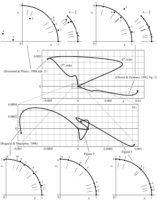
Figure 9: One step $h=\frac{\pi}{2}$ for the system ${\rm d}x/{\rm d}\mkern 1.0mut=-y$, ${\rm d}y/{\rm d}\mkern 1.0mut=x$ with initial conditions $x(0)=1$, $y(0)=0$: the intermediate positions ${\boldsymbol{X}}_{\mkern-1.0mui}$, $1\leq i\leq s$, and the error $\bigl{(}x(\frac{\pi}{2}\theta)-\cos(\frac{\pi}{2}\theta),\,y(\frac{\pi}{2}\theta)-\sin(\frac{\pi}{2}\theta)\bigr{)}$, where $0\leq\theta\leq 1$, made by an interpolant. Nodes are shown by the radial ticks. Open circles correspond to additional stages that are used to construct an interpolant. Ticks on the error curves correspond to $\theta=\frac{1}{12}$, $\frac{1}{6}$, $\frac{1}{4}$, …, $\frac{11}{12}$. In case of the (Dormand & Prince, 1980, tab. 2) pair, the ${5}^{\textrm{th}}$ order interpolant is the (Calvo et al., 1990) one, while the ${4}^{\textrm{th}}$ order interpolant with $u=s=7$ is from

ntrp45.m

code that is a part of MATLAB^® software.

​Figure 9 shows the performance of five pairs and their interpolants on the system ${\rm d}x/{\rm d}t=-y$, ${\rm d}y/{\rm d}t=x$ with initial condition $\bigl{(}x(0),y(0)\bigr{)}=(1,0)$. Just one step $h=\frac{\pi}{2}$ is made, with no error control. The exact solution is $x(t)=\cos t$, $y(t)=\sin t$ with $\bigl{(}x(\frac{\pi}{2}),y(\frac{\pi}{2})\bigr{)}=(0,1)$. In cases of the (Dormand & Prince, 1980, tab. 2) and (Owren & Zennaro, 1992, fig. 3) pairs the intermediate positions ${\boldsymbol{X}}_{\mkern-1.0mui}$, $1\leq i\leq s$, are also shown for the step size $h=\frac{\pi}{4}$. For the (Dormand & Prince, 1980, tab. 2) pair, $({\boldsymbol{q}}_{2})_{i}=0$ for all $i\neq 2$. In the leading order the deviation of ${\boldsymbol{X}}_{\mkern-1.0mui}$ from ${\boldsymbol{x}}(t+c_{\mkern 0.5mui}\mkern 1.0muh)$ is controlled by $T_{3}({\boldsymbol{a}}_{i*},c_{i})=\bigl{|}\mkern 0.5mu{\boldsymbol{a}}_{i*}\mkern 1.0mu{\boldsymbol{A}}\mkern 1.0mu{\boldsymbol{c}}-c_{i}^{3}/6\bigr{|}$ that for $i=3$, $4$, $5$, and $6$ is equal to $\frac{9}{2000}=0.0045$, $\frac{28}{375}=0.0746...$, $\frac{2536}{10935}=0.231...$, and $\frac{71}{330}=0.215...$, respectively. Relatively large values of $T_{3}({\boldsymbol{a}}_{5*},c_{5})$ and $T_{3}({\boldsymbol{a}}_{6*},c_{6})$ explain the observed deviation of ${\boldsymbol{X}}_{\mkern-1.0mu5}$ and ${\boldsymbol{X}}_{\mkern-1.0mu6}$ from $\bigl{(}\cos\frac{8\mkern 0.5muh}{9},\,\sin\frac{8\mkern 0.5muh}{9}\bigr{)}$ and $(\cos h,\,\sin h)$. Even for $h=\frac{\pi}{2}$ the position update ${\boldsymbol{x}}(t+h)={\boldsymbol{X}}_{\mkern-1.0mu7}$ is remarkably close to the exact value, though.

5 Conclusion

Utilizing $9$ stages, it is possible to construct embedded $(4,5)$ pairs of explicit Runge–Kutta methods with FSAL property that are as cost-efficient as the best known conventional (i.e., interpolant is either of order $4$ or would require extra stages) pairs (e.g., the Dormand–Prince and Bogacki–Shampine ones), but with the benefit of having continuous formulae or interpolants of order $5$ available at no additional cost.

References

- Ascher & Petzold (1998) Ascher, U. M. & Petzold, L. R. (1998) Computer methods for ordinary differential equations and differential-algebraic equations, SIAM.
- Bogacki (1990) Bogacki, P. (1990) Efficient Runge–Kutta pairs and their interpolants. Ph.D. thesis, Department of Mathematics, Southern Methodist University, Dallas, TX, USA.
- Bogacki & Shampine (1996) Bogacki, P. & Shampine, L. F. (1996) An efficient Runge–Kutta pair. Computers & Mathematics with Applications, 32 (6) 15–28.
- Brankin et al. (1993) Brankin, R. W., Gladwell, I. & Shampine, L. F. (1993) RKSUITE: A suite of explicit Runge-Kutta codes. Contributions in numerical mathematics, ed. R. P. Agarwal, World Scientific, pp. 41–53.
- Butcher (1964) Butcher, J. C. (1964) On Runge–Kutta processes of high order. Journal of the Australian Mathematical Society, 4 (2) 179–194.
- Butcher (2008) Butcher, J. C. (2008) Numerical methods for ordinary differential equations, 2nd ed., John Wiley & Sons Ltd.
- Butcher & Wanner (1996) Butcher, J. C. & Wanner, G. (1996) Runge–Kutta methods: some historical notes. Applied Numerical Mathematics, 22 (1–3) 113–151.
- Calvo et al. (1990) Calvo, M., Montijano, J. I. & Randez, L. (1990) A fifth-order interpolant for the Dormand and Prince Runge–Kutta method. Journal of Computational and Applied Mathematics, 29 (1) 91–100.
- Dormand et al. (1989) Dormand, J. R., Lockyer, M. A., McGorrigan, N. E. & Prince, P. J. (1989) Global error estimation with Runge–Kutta triples. Computers & Mathematics with Applications, 18 (9) 835–846.
- Dormand & Prince (1978) Dormand, J. R. & Prince, P. J. (1978) New Runge–Kutta algorithms for numerical simulation in dynamical astronomy. Celestial Mechanics, 18 (3) 223–232.
- Dormand & Prince (1980) Dormand, J. R. & Prince, P. J. (1980) A family of embedded Runge-Kutta formulae. Journal of Computational and Applied Mathematics, 6 (1) 19–26.
- Enright et al. (1986) Enright, W.H., Jackson, K. R., Nørsett, S. P. & Thomsen, P. G. (1986) Interpolants for Runge–Kutta formulas. ACM Transactions on Mathematical Software, 12 (3) 193–218.
- Fehlberg (1969) Fehlberg, E. (1969) Low-order classical Runge–Kutta formulas with stepsize control and their application to some heat transfer problems. NASA Technical Report R-315.
- Fehlberg (1970) Fehlberg, E. (1970) Klassische Runge–Kutta-Formeln vierter und niedrigerer Ordnung mit Schrittweiten-Kontrolle und ihre Anwendung auf Wärmeleitungsprobleme. Computing 6, 61–71.
- Hairer et al. (2008) Hairer, E., Nørsett, S. P. & Wanner, G. (2008) Solving ordinary differential equations I: nonstiff problems, 2nd ed., Springer.
- Horn (1983) Horn, M. K. (1983) Fourth- and fifth-order, scaled Runge–Kutta algorithms for treating dense output. SIAM Journal on Numerical Analysis, 20 (3) 558–568.
- Hull et al. (1972) Hull, T. E., Enright, W.H., Fellen, B. M. & Sedgwick, A. E. (1972) Comparing numerical methods for ordinary differential equations. SIAM Journal on Numerical Analysis, 9 (4) 603–637.
- Iserles (2009) Iserles, A. (2009) A first course in the numerical analysis of differential equations, 2nd ed., Cambridge University Press.
- Owren & Zennaro (1991) Owren, B. & Zennaro, M. (1991) Order barriers for continuous explicit Runge–Kutta methods. Mathematics of Computation, 56 (194) 645–661.
- Owren & Zennaro (1992) Owren, B. & Zennaro, M. (1992) Derivation of efficient, continuous, explicit Runge–Kutta methods. SIAM Journal on Scientific and Statistical Computing, 13 (6) 1488–1501.
- Sarafyan (1984) Sarafyan, D. (1984) Continuous approximate solution of ordinary differential equations and their systems. Computers & Mathematics with Applications, 10 (2) 139–159.
- Shampine (1986) Shampine, L. F. (1986) Some practical Runge–Kutta formulas. Mathematics of Computation, 46 (173) 135–150.
- Sharp & Smart (1993) Sharp, P. W. & Smart, E. (1993) Explicit Runge–Kutta pairs with one more derivative evaluation than the minimum. SIAM Journal on Scientific Computing, 14 (2) 338–348.
- Sharp & Verner (1994) Sharp, P. W. & Verner, J. H. (1994) Completely imbedded Runge–Kutta pairs. SIAM Journal on Numerical Analysis, 31 (4) 1169–1190.
- Verner (1978) Verner, J. H. (1978) Explicit Runge–Kutta methods with estimates of the local truncation error. SIAM Journal on Numerical Analysis, 15 (4) 772–790.
- Verner (1991) Verner, J. H. (1991) Some Runge–Kutta formula pairs. SIAM Journal on Numerical Analysis, 28 (2) 496–511.
- Verner (1993) Verner, J. H. (1993) Differentiable interpolants for high-order Runge–Kutta methods. SIAM Journal on Numerical Analysis, 30 (5) 1446–1466.
- Verner (2010) Verner, J. H. (2010) Numerically optimal Runge–Kutta pairs with interpolants. Numerical Algorithms, 53 (3) 383–396.
- Verner & Zennaro (1995) Verner, J. H. & Zennaro, M. (1995) Continuous explicit Runge–Kutta methods of order . Mathematics of Computation, 64 (211) 1123–1146.