Galaxy Spectra neural Networks (GaSNets). I. Searching for strong lens candidates in eBOSS spectra using Deep Learning

Abstract

With the advent of new spectroscopic surveys from ground and space, observing up to hundreds of millions of galaxies, spectra classification will become overwhelming for standard analysis techniques. To prepare for this challenge, we introduce a family of deep learning tools to classify features in one-dimensional spectra. As the first application of these Galaxy Spectra neural Networks (GaSNets), we focus on tools specialized in identifying emission lines from strongly lensed star-forming galaxies in the eBOSS spectra. We first discuss the training and testing of these networks and define a threshold probability, $P_{L}$, of 95% for the high-quality event detection. Then, using a previous set of spectroscopically selected strong lenses from eBOSS, confirmed with HST, we estimate a completeness of $\sim$80% as the fraction of lenses recovered above the adopted $P_{L}$. We finally apply the GaSNets to $\sim 1.3$M eBOSS spectra to collect the first list of $\sim$430 new high-quality candidates identified with deep learning from spectroscopy and visually graded as highly probable real events. A preliminary check against ground-based observations tentatively shows that this sample has a confirmation rate of 38%, in line with previous samples selected with standard (no deep learning) classification tools and confirmed by the Hubble Space Telescope. This first test shows that machine learning can be efficiently extended to feature recognition in the wavelength space, which will be crucial for future surveys like 4MOST, DESI, Euclid, and the China Space Station Telescope (CSST).

1 Introduction

Strong gravitational lensing (SGL) is a powerful tool to investigate a large variety of open questions in cosmology. The formation of the distorted images of background galaxies, the “sources”, depends on the total mass of the foreground gravitational systems acting as “deflectors” or “lenses”. In case this latter are galaxies, SGL provides us accurate constraints on different properties correlated to their total mass, like the mass-to-light ratio (Ghosh et al. 2021), the dark matter fraction (Auger et al. 2009; Tortora et al. 2010), the slope of the total density profile (Koopmans et al. 2006, 2009, Auger et al. 2009) and its relation with other parameters (Bolton et al. 2012, Shu et al. 2015; Li et al. 2018). SGL is also used to constrain the evolution of galaxies via merging (Bolton et al. 2012, Sonnenfeld et al. 2013, 2014, 2015), the initial mass function in massive ellipticals (Spiniello et al. 2011; Barnabè et al. 2012), and study the dark substructures around large galaxies (Gilman et al. 2018; Schuldt et al. 2019).

Moving to more cosmological constraints, SGL is used to measure the Hubble constant($H_{0}$), and other cosmological parameters (Suyu et al. 2013, 2017; Sluse et al. 2019; Rusu et al. 2020; Wong et al. 2020).

Strong lenses are generally searched in imaging data, where one can clearly distinguish the lensing features in the form of arcs, or multiple images of compact sources, like galaxies or quasars (Bolton et al. 2008; Brownstein et al. 2012; Sonnenfeld et al. 2013; Suyu et al. 2013). Here, a great impulse to lens hunting has been recently provided by automatized tools for lens finding (Gavazzi et al. 2014). In particular, machine learning (ML) techniques have been lately found to be very powerful in collecting hundreds of high quality (HQ) candidates (Dark Energy Survey – DES: Jacobs et al. 2019, Kilo Degree Survey – KiDS: Petrillo et al. 2019; Li et al. 2020, 2021b, Hyper Supreme-Cam – HSC: Sonnenfeld et al. 2018).

After the identification of HQ candidates, a spectroscopical follow-up is needed to confirm their gravitational lensing nature (Metcalf et al. 2019; Witstok et al. 2021). In practice, one needs to collect the spectra of the lens and the source and measure their relative redshift, confirming that the lens is located in front of the source as expected from ray-tracing lensing models (see Cornachione et al. 2018, Napolitano et al. 2020). This is a severe bottleneck in the SGL studies and, so far, there have been only sparse programs dedicated to these follow-up observations (Spiniello et al. 2019a, b; Lemon et al. 2020; Nord et al. 2020). However, future large sky spectroscopic surveys (e.g. Taipan: da Cunha et al. 2017 4MOST: de Jong et al. 2012, DESI: DESI Collaboration et al. 2016) will provide an unprecedented opportunity for massive follow-ups of lensing candidates, e.g. by reserving them dedicated observing nieces in wide programs or by accommodating them as filler targets in large-sky, multi-purpose surveys.

More interestingly, these large spectroscopic sky surveys will offer a unique chance to be used as a playground for lens finding, e.g. by looking for blended emission lines of background “lensed” galaxies, e.g. star-forming systems, in the spectrum of a forward massive systems. This method has been extensively used in the last years to produce tens of discoveries of new unknown lens candidates.

The first example of a search of this kind was presented by Bolton et al. (2004), within The Sloan Lens ACS (SLACS). They found 49 SGL candidates in 50 996 Sloan Sky Digital Survey (SDSS) spectra of luminous red galaxies (LRG). They used the principal-component analysis to subtract the main components of the foreground LRG spectrum and a Gaussian kernel to find the best emission lines in the residual flux. They mainly focused on [OII] (3728Å), [OIII] (4960Å, 5007Å), and $H_{\beta}$ (4863Å) lines, hence exploring a redshift range of $z=(0.16-0.49)$ for the lenses and $z=(0.25-0.81)$ for the sources. Later analyses increased the number of SLACS candidates to 131 (Bolton et al. 2008, SLACS hereafter). Within the BOSS Emission-Line Lens Survey (BELLS, hereafter), Brownstein et al. (2012) extended the spectroscopic search, previously performed in SLACS, to higher redshift, by looking for lenses up to $z=0.7$ and the background sources up to $z=1.4$, with no color pre-selection. This allowed them to finally find 45 SGL candidates in 133 852 SDSS galaxy spectra. Along the same line of approaches, in the SLACS Survey for the Masses (S4TM) project, Shu et al. (2015, 2017, S4TM hereafter) have extended the search for SGL candidates to lower masses and found 118 new lens candidates. On the other hand, Shu et al. (2016a, b, BELLS GALLERY) and Cao et al. (2020) looked for high-redshift Ly$\alpha$ emitters as background sources and found 361 candidates.

The main disadvantage of these spectroscopy-selected samples is the missing information from images. Indeed, even if spectra can provide the evidence of two different emitting sources along the line of sight located at different redshifts, they cannot guarantee that they represent an SGL event. Hence, high-resolution imaging from space telescopes or adaptive optics is needed to have a visual confirmation of the lenses. Currently, there are 135 confirmed lenses with Hubble Space Telescope (HST) observations of the 294 selected using optical lines (70/131 from SLACS, 25/45 from BELLS, 40/118 from S4TM), and 17/21 Ly$\alpha$ candidates from BELLS GALLERY.

With the lesson learned from SDSS/BOSS, other experiments have combined the spectroscopic selection and imaging: Chan et al. (2016) matched 45 spectra from the Galaxy And Mass Assembly (GAMA) survey and confirmed 10 of them with Hyper Suprime-Cam (HSC) imaging; Holwerda et al. (2022) selected lens candidates in AAOmega spectra and followed up 56 of them with HST to find 9 confirmations.

The discovery power of this approach will be pushed to unprecedented limits by future surveys combining spectroscopy and imaging from space (e.g. Euclid mission and CSST) and produce a revolution in the lensing searches. However, this revolution will stand on the ability to effectively analyze gigantic spectroscopic data loads, which will imply the inspection of millions of spectra and the identification of (sometimes very faint) emission lines from background lensed systems. This is a prohibitive task for standard human-driven analyses, unless one adopts severe selections to maximise the number of detection but reduce the spectra to visually inspect.

Machine learning techniques can provide, instead, fast and efficient methods to overcome these difficulties and systematically search for lensing features in spectra. For instance, Convolutional Neural Networks (CNNs) have been previously applied for lens searches (see Li et al. 2019, Li+19, hereafter). In particular, they have focused on the identification of Ly$\alpha$ emitters at higher redshift ($2<z<3$) in the spectra of lower redshift early-type galaxies ($z<0.6$), and showed that these techniques can be efficiently used as a classifier for galaxy spectra.

In this paper, we expand this approach and develop a new CNN tool to look for SGL in the Baryon Oscillation Spectroscopic Survey (BOSS) spectroscopic database (Dawson et al. 2016). Since these sources are usually star-forming galaxies, we plan to use machine learning techniques to search for higher redshift emission lines such as [OII], [OIII], $H_{\alpha}$, $H_{\beta}$ and $H_{\delta}$ mixed in the foreground galaxy spectra. To do that, we build 3 CNN models: a classifier, to search for reliable emission lines in spectra, and two regression models, to measure the foreground galaxy and the background source redshifts, respectively. Then, we combine the predictions of the 3 CNNs to provide a list of high probability events that we visually inspect to select HQ candidates.

Finally, we compare this first deep learning spectroscopic-selected sample with the most complete spectroscopic sample of SGL candidates in BOSS observations from Talbot et al. (2021, T+21 hereafter), obtained with standard cross-correlation techniques. This catalog consist of 838 likely, 448 probable, and 265 possible strong lens candidates, for a total of 1551 objects. They have also obtained a preliminary confirmation of 477 of them with low-resolution imaging.

The paper is organized as follows. In §2, we will introduce the whole idea of this project and the details of the new CNN models. In §3, we introduce the modeled emission lines and the construction of training data. In §4, we show the training and testing results of the new CNNs. In §5, we will apply the new CNNs to the BOSS spectra and derive a list of candidates that we qualify via visual inspection of their spectra, finally providing a catalog of HQ candidates. In §6, we will discuss the results and estimate a tentative confirmation rate based on the match with ground-based imaging. We also discuss some avenues for improvement of future CNNs. In the final §7, we draw some conclusions.

2 Methodology

In this work we want to apply ML techniques to spectroscopic data. In particular, we want to use the ability of these techniques to perform feature recognition and classification. ML has been widely used in astronomical data analysis: 1) to find or classify different astronomical target candidates, like AGN (Teimoorinia & Keown 2018; Zhu et al. 2021; Chang et al. 2021), quasar (Khramtsov et al. 2019; Yang et al. 2021), star clusters (Jadhav et al. 2021; He et al. 2021) or 2) to measure or predict physical parameters of astronomical targets, like redshifts (Ball et al. 2007; Han et al. 2021), masses (Ntampaka et al. 2016; Bonjean et al. 2019), or velocity profiles (MacBride et al. 2021). Here we want to test the possibility to use ML techniques to efficiently search for strong lenses on vast amounts of spectra and predict the redshift of their lenses and sources.

2.1 The challenge of searching for strong lenses in spectra

Next generation spectroscopic surveys will target tens of millions of galaxies (Mandelbaum et al. 2019). These huge samples will allow us to systematically search for high-probability candidates from integrated spectra, as the number of expected events is noticeable, given the large number of background galaxies potentially giving rise to lensing events.

Using the set of predictions from Collett (2015), we have estimated that the number of lenses with a $1^{\prime\prime}$ Einstein radius, $R_{\rm E}$, producing lensed images of the source, observable with a spectroscopic survey with a 2^′′ diameter fiber, over 15 000 deg² of the sky, is of the order of 7 000. This is obtained assuming that the source is bright enough in some visual band (e.g. Euclid visual mag$=24.5$) to make also the signal-to-noise ratio of the emission lines high enough to be detected from the ground for typical spectroscopic surveys (e.g. 4MOST or DESI). This estimate is subject to different factors, including some flux loss, but it also excludes the contribution from sources with slightly larger $R_{\rm E}$s that might eventually scatter part of their light into a 2^′′ fiber. Hence, combining all these effects, this forecast is possibly not far from realistic. This is a wealth of data extremely valuable because it provides, for free, the information on the lens and the source redshifts, which are crucial for the lensing modeling. Standard techniques based on sophisticated selection criteria (T+21) still require rather time-consuming visual inspection. Hence, a more practical solution to perform a systematic search of lens candidates in these datasets is mandatory.

This is possibly true also for current spectroscopic surveys. For instance, using the same set of predictions for the BOSS area ($\sim 10000$ deg²), and assuming a fainter limiting magnitude for the sources, $r=$23.5, we get $\sim 920$ lenses within a 2^′′ fiber, which become $\sim 1470$ within a 3^′′ fiber (e.g. the one available for SDSS releases earlier than 12). Currently, the largest collection of candidate lenses with BOSS spectra consists of 477 objects with lensing evidence from low-resolution images (T+21). Taking this sample as a bona fide high-completeness sample, this is rather far from the expected number of discoverable lenses, meaning that there might be more lenses to find in the full BOSS dataset. Given the full set of BOSS spectra available, i.e. $\sim 2.6$M items (Ahumada et al. 2020), this means that we should expect one real blended emission line object every $\sim$3500 spectra.

In this work, we want to tackle the problem of systematic searches of lens candidates in spectra with deep learning and use the BOSS dataset to test the efficiency of this approach.

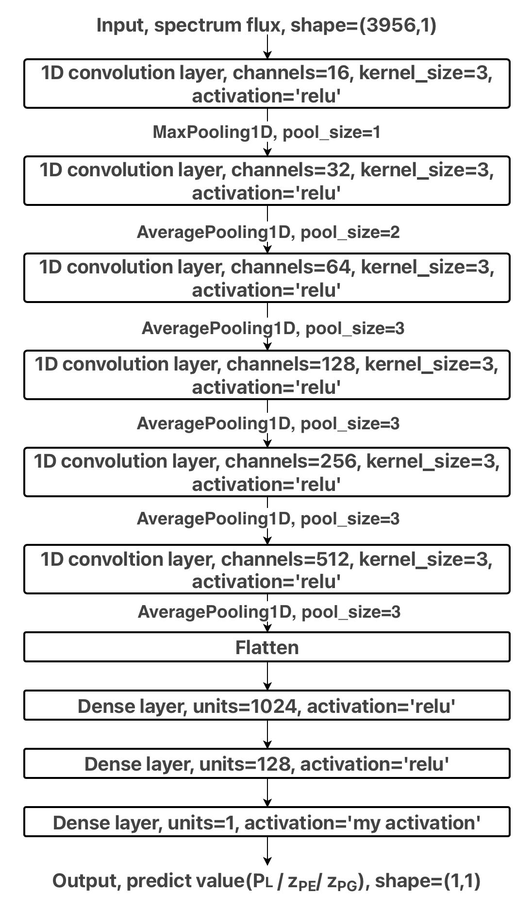
Figure 1: The CNN model adopted for the GasNet-L1, L2, and L3. The network structure is the same for the three GaSNets, except for the activation and loss functions as reported in Table 1.

2.2 Convolutional Neural Networks as lens classifiers in 1D spectra

When searching for strong lens candidates in 1-dimension (1D) spectra, one needs to identify two main features: 1) the potential emission lines from the background sources, to determine the redshift of the source, and 2) the absorption or emission lines of the foreground galaxies, to determine the redshift of the lens and compare this with one of the putative sources to possibly qualify the whole system as a lensing candidate. In most of the current and planned surveys, the redshift of the main galaxy (the lens) is a standard data product, hence this can be assumed to be a label of the spectroscopic catalog. This can be either used as a first guess for the lens classifier, to estimate the lens redshift itself or kept fixed, asking the CNN to identify tentative background lines (see below).

2.3 Galaxy Spectra convolutional neural Networks (GaSNets)

In this work, we present the first set of Galaxy Spectra convolutional neural Networks (GaSNets) for Lensing (-L). These are CNNs trained to identify strong lensing event candidates in 1D galaxy spectra. To perform this task, we have built three different GaSNet models:

1. GaSNet-L1. This CNN is a classifier, trained to look for the presence of emission lines blended in the features of the foreground galaxy and give the probability to be a lens ($P_{L}$). In doing this, we do not assume any specific morphology for the lens, which can be either a standard early-type galaxy (ETG), dominated by absorption line features, or a late-type galaxy (LTG), with ongoing star-formation. The GaSNet-L1 will learn whether, in the spectra of either kind, there are higher-redshift emission lines, to finally give the $P_{L}$.

2. GaSNet-L2. This CNN is a regression algorithm, trained to identify potential emission lines, among a list of standard features from star-forming galaxies, overlapping a foreground galaxy spectrum and predict their redshift ($z_{PE}$).

3. GaSNet-L3. This CNN is also a regression algorithm, trained to predict the redshift of the foreground galaxy ($z_{PG}$) from the combination of continuum plus a) classical absorption features from ETG spectra or b) emission lines of LTGs. Having such an output will make the overall Network general enough to be applied to spectroscopic databases, regardless these have gone through a pipeline to estimate galaxy redshifts. In our analysis below, even though we can assume that the redshift of the lenses is given (as they are provided with the BOSS spectra, see Sect. 3.1), we opt to use the redshift predictions of our GaSNet-L3 for the candidate selection and use the BOSS redshifts as ground truth to assess the accuracy of the deep learning estimates.

The three CNN models have the same structure. They are built by 6 convolution layers and 3 total connected layers (see Fig. 1), assembled by Python modules TensorFlow and Keras. In the last layer in Fig. 1, due to the different tasks to perform (classification vs. regression), for GaSNet-L1 we use a “sigmoid” activation function (labeled as “my activation”), while for GaSNet-L2 and L3 we need no activation. For the same reason, we also use different loss functions. For GaSNet-L1 we adopt a “binary cross-entropy” loss, which is commonly used for a binary classifier. For GaSNet-L2 and GaSNet-L3, which are two regression models, instead of the commonly used MAE and MSE loss functions, we apply the “Huber” loss. This is defined as

$$L_{\delta}(a)=\begin{cases}\dfrac{1}{2}(a)^{2},\ \ \ |a|\leq\delta\\ \delta\cdot(|a|-\dfrac{1}{2}\delta),\ \ \ {\rm otherwise}.\end{cases}$$ (1)

where $a=y_{\rm true}-y_{\rm pred}$, $y_{\rm true}$ is the real redshift, $y_{\rm pred}$ is the predicted redshift by the CNNs , and $\delta$ is a parameter that can be preset ($0.001$ in this work). The choice of the “Huber” Loss has been made because, as shown in CNN regression models for galaxy light profiles (i.e. the GaLNets, Li et al. 2021a), it can achieve higher accuracy than MAE and MSE and better convergence. Both “activation” and “loss functions” are summarized in Table 1.

Table 1: CNN “my activation” and “loss function”

	GaSNet-L1	GaSNet-L2	GaSNet-L3
my  activation	sigmoid	-	-
loss  function	binary  crossentropy	huber_loss	huber_loss

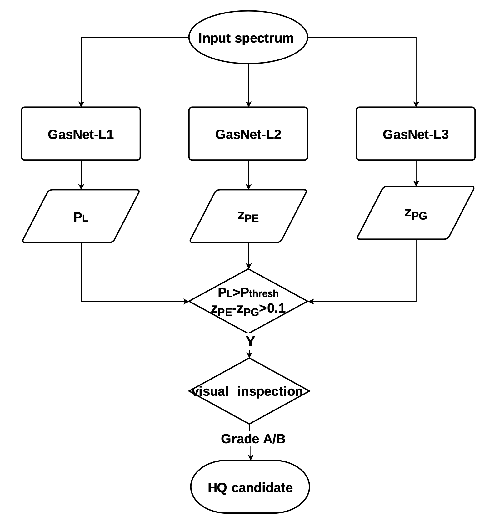
Figure 2: Flow-chart describing the process to obtain the HQ candidates combining the output of the three GaSNets. The final step is the visual inspection of the candidates selected using the probability criterion, $P_{L}>P_{\rm thresh}$, combined with the presence of background emission lines, $z_{PE}>z_{PG}+0.1$.

From Fig. 1 we see that the CNNs all accept a 1D spectrum (i.e. a vector of wavelength and fluxes) as input and produce as predicted parameters, either a probability ($P_{L}$ for GaSNet-L1) or a redshift (i.e. $z_{PE}$ and $z_{PG}$ for GaSNet-L2 and GaSNet-L3, respectively).

2.4 Decomposing a complex CNN model

To conclude this section, we briefly discuss the choice to combine the outcome of three CNNs to improve the accuracy of the identification of high-quality (HQ) candidates and minimize the chance of false detection.

This task involves two steps: 1) the identification of different kinds of features that can suggest the presence of a lensing event, i.e. the coexistence of absorption and emissions lines from different objects along the line-of-sight, and 2) the verification that (some of) the emission lines come from the background system. This is a complex classification task that can be more efficiently performed by combining different CNNs with different specializations. Indeed, GaSNet-L1 is designed to identify a specific series of emission lines at a higher redshift overlying a lower redshift spectrum characterized either by a continuum plus absorption lines typical of ETGs or continuum plus emission lines from LTGs. Even if the training sample is made of real galaxy spectra, where the simulated emission lines from mock background sources are randomly redshifted with respect to the main galaxy (see §3), GaSNet-L1 can only give a probability of the coexistence of a lens and a source at different redshifts, but cannot predict by how much the emissions of the source are misplaced. Since this process can be uncertain, we cannot exclude that GaSNet-L1 can confuse a lensing event with other “local” emission processes (e.g. active galactic nuclei, ongoing star-formation, gas outflows, etc.), and vice versa. On the other hand, the GaSNet-L2 and GaSNet-L3 are able to predict the redshift of the tentative source and lens, independently, meaning that they cannot predict, individually, if there is another object at a different redshift, compatibly with a lensing event.

Only using the outputs of these three GaSNets together, we can both give a “high probability” that there are two different systems contributing to the spectrum and establish that the closer one is a galaxy, with redshift $z_{PG}$, and the background one is a fainter line emitter, with redshift $z_{PE}$. In particular, to qualify a spectrum as a candidate, we use the following conditions: 1) $P_{L}>P_{\rm thresh}$, and 2) $z_{PE}>z_{PG}$, where $P_{\rm thresh}$ is an appropriate lower probability threshold that will be chosen later to define the high-probability candidates that will be further visually investigated to assemble the list of candidates to pass to the visual inspection, which finally produces the HQ candidate list. The full process for the selection and grading of the HQ candidates is schematized in Fig. 2.

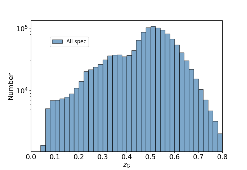
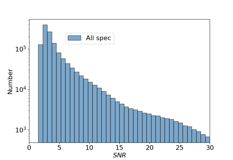
Figure 3: The redshift and SNR distribution of the DR16-predictive sample (see text for details).

3 Data

The construction of the training sample is a critical step of any supervised ML algorithm. Indeed, to avoid biased predictions and fictitious performances, the training samples need to be as close as possible to real observations. In our case, we build our training sample starting from real spectra from BOSS, over which we simulate the presence of emission lines. Here below, we first introduce the dataset we use for our analysis. Then, we describe the way we have constructed the training set. This is constituted by two samples.

First, the negative sample, which represents a catalog of galaxy spectra with no background sources blended in. As mentioned earlier, we do not make any selection of galaxy types and we include ETGs and LTGs.

Second, the so-called positive sample, which represents a simulated sample of spectra that emulates the presence of emission lines from a background source. This is made of the same galaxy spectra of the negative sample, but with the addition of artificial emission lines, redshifted with respect to the “foreground” galaxies.

3.1 Data selection and predictive sample

The Sloan Digital Sky Survey (SDSS, see York et al. 2000) has observed over 10 000 deg² of the sky, performing multi-band photometry and spectroscopy (Szalay et al. 1999). In 2009, before the start of the Baryon Oscillation Spectroscopic Survey (BOSS, Schlegel et al. 2009), in the third stage of the project (SDSS-III), the spectrograph operating the observations has been upgraded. Compared to SDSS-I/II, the number of fibers was increased from 640 to 1000, and the fiber diameter has been reduced from 3^′′ to 2^′′ (Ahn et al. 2012). The extended version of the BOSS survey, eBOSS (Dawson et al. 2016), has overall produced spectra for around 2.6 million galaxies, in the wavelength range 361–1014 nm. These are publicly available through the latest data release 16 (DR16, Ahumada et al. 2020). This is the dataset we use in this work, over which we operate a series of selections to ensure the quality of the spectra to analyze. In particular, we select only: 1) plates labeled as “good” quality, 2) “Object” flags labeled as “galaxy”, 3) spectroscopic redshift between $0.05-0.8$, 4) spectra with SNR$>2$, 5) wavelength range 3700–9200Å.

Table 2: Model parameters of equation 2.

	$\lambda_{e,1}$	$\lambda_{e,2}$	$h_{e}$	$z_{max}$
$[OII]^{1}$	3726.2	3728.9	[2,10]	1.44
[OIII]	4959.0	n/a	[1,5]	0.82
[OIII]	5007.0	n/a	[1,15]	0.82
$H_{\alpha}$	6562.8	n/a	[1,15]	0.39
$H_{\gamma}$	4340.5	n/a	[1,5]	1.10
$H_{\beta}$	4861.3	n/a	[1,5]	0.87

This latter criterion is applied to avoid a rather noisy region of the spectra, at $\lambda>9200$Å, where the residuals from the telluric line subtraction might be a source of spurious detections. This is a problem we expect to deal with in future developments, but we wanted to avoid in this first test. We stress, though, that the reduced wavelength range will allow us to train tools that can be straightforwardly applicable to the SDSS-I/II spectra, whose wavelength range is also limited to 3700-9200Å. Of course, this makes our tools less sensitive to higher-$z$ systems, as many of the emission lines we want to detect will fall out of the range at redshift z $>$$\sim$1.4 (see below).

Criterion 3 is dictated by the line observability. Indeed, we will assume that typical sources in the SGL events are star-forming galaxies characterized by emission lines as reported in Table 2. Here, for each line, we list the central wavelength(s), the maximum redshift the emission line can reach below 9200Å, $z_{\rm max}$, and an intensity parameter, $h_{e}$, that will be used in §3.3 for the simulated spectra. According to this list, for redshift $z_{E}\leavevmode\nobreak\ \hbox to0.0pt{$>$\hss}{\lower 4.30554pt\hbox{$\sim$}}1.4$, all lines would fall out of the eBOSS wavelength range, while with $z_{E}\mathrel{\hbox to0.0pt{\lower 3.5pt\hbox{\hskip 0.5pt$\sim$}\hss}\raise 0.5pt\hbox{$<$}}1.2$, we can still retain two emission lines, i.e. [OII] and $H_{\gamma}$. In order to select lenses that are compatible with the visibility of the background lines and with a reasonable lens-source distance to guarantee an SGL event, we collect spectra in the range $z_{G}=(0.05\sim 0.8)$.

Criterion 4, on the other hand, is an optimistic lower limit we have chosen to increase the completeness. We have considered that the emission lines from background sources have a SNR which is not necessarily correlated to the SNR of the whole spectrum and, thus, can be seen also in a noisy galaxy spectrum.

The final selected sample consists of $1\,339\,895$ spectra: in the following, we will refer to this as the DR16-predictive sample. In Fig. 3 we show the SNR distribution of the selected spectra and the redshift of the central galaxy.

3.2 Construction of the negative sample

The first step to produce our training dataset is the selection of the negative sample. This is chosen to make the CNN as general as possible, hence assuming that every type of galaxy can work as a lens, with no particular restrictions in luminosity or color, as it is typically done to contain the predictive samples in imaging classifiers (see e.g. Petrillo et al. 2019, Li et al. 2020).

For this purpose, we select 140 000 galaxies spectra from the DR16-predictive sample, with a wavelength range of 3700-9200 Å. We take particular care that the selected spectra uniformly cover, in number, the full $z_{G}$ range, by counting the spectra in redshift bins of 0.05. This is crucial to avoid any bias in the prediction of the $z_{G}$ from the poor sampling of one redshift bin with respect to the close ones.

To mimic the presence of emission lines from local processes, for 1/5 of the negative sample, we add artificial emission lines with the same redshift of the galaxy, while the remaining 4/5 of the negative sample is left unchanged. In particular, for this simulated “local emissions”, we use the same lines, reported in Table 2, that will be used to simulate the background source emissions, which we expect the GaSNets to distinguish from the local ones (if any).

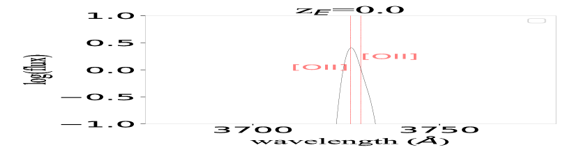
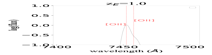
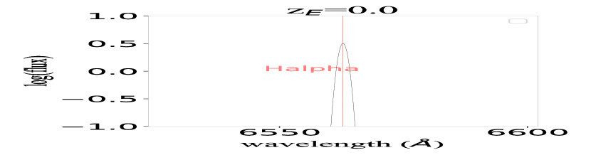
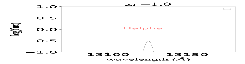
Figure 4: Detail of the line profiles of the simulated emissions. Artificial Oxygen, OII (3727.1Å and 3729.9Å) lines (top) and Halpha (6562.8Å) lines (bottom), as observed at different redshifts. The line fluxes are redshifted and dimmed according to Eqs. 4-6.

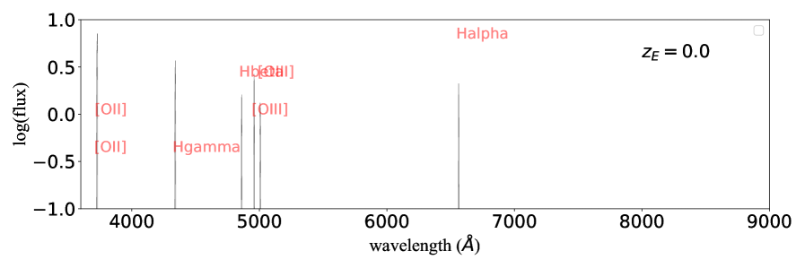
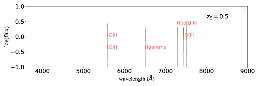
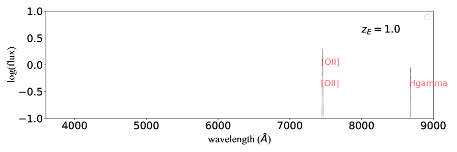
Figure 5: Full spectrum of artificial emission lines added to the negative sample (see Table 2 and text for details). The line fluxes are redshifted and dimmed according to Eqs. 4-6.

3.3 Artificial emission line model

In this section, we give more details about the artificial emission lines we want to add to the original eBOSS spectra to emulate both some local and higher-$z$ emissions in the negative and positive samples, to be used for the CNN training. Following Li+19, we use a 1-dimensional “double gaussian” profile, defined as:

$$F(\lambda)=h_{1}\exp\{-\frac{(\lambda-\lambda_{e,1})^{2}}{2\sigma_{1}^{2}}\}+h_{2}\exp\{-\frac{(\lambda-\lambda_{e,2})^{2}}{2\sigma_{2}^{2}}\}$$ (2)

where $F$ is the flux, $\lambda_{e,1}$ and $\lambda_{e,2}$ are the central wavelengths of the emission lines, and $h_{1}$, $h_{2}$, $\sigma_{1}$, $\sigma_{2}$ are the four model parameters. The $\lambda_{e,1}$, $\lambda_{e,2}$, $h_{1}$, and $h_{2}$ are listed in Table 2. These parameters are further defined to satisfy the following conditions:

$$\begin{cases}\sigma_{1}\in[0.8,1.6]\\ \sigma_{2}\in\sigma_{1}+[0.5\sigma_{1},1\sigma_{1}]\\ h_{1}=\frac{h_{e}}{(1+z_{E})^{2}}\\ h_{2}=\frac{h_{e}}{4(1+z_{E})^{2}}\rm\leavevmode\nobreak\ if\leavevmode\nobreak\ \lambda_{e,2}\neq n/a;&=0\leavevmode\nobreak\ \rm otherwise\\ \end{cases}$$ (3)

where the $\sigma_{1}$ is uniformly selected in the interval $[0.8,1.6]$, the amplitude parameter, $h_{e}$, is given in Table 2, and $z_{E}$ is the redshift of the emission line we want to simulate, assumed to be uniform in the range [$z_{G}+0.1$, 1.2]

The $\sigma_{1}$ range is determined under the assumption that the emission lines from sources are enlarged by rotation. Hence, the line broadening in wavelength can be written as $\Delta\lambda\approx 2\lambda_{0}v_{r}/c$, where $\lambda_{0}$ is the central wavelength of the emission line, $v_{r}$ is the max velocity along the line-of-sight, and $c$ is the speed of light. Then, we can approximate $2\sigma_{1}\approx\Delta\lambda$, which, for a rotation $v_{r}\sim 100$ km/s and $\lambda_{0}\approx 370$nm, gives $\sigma_{1}\approx 1.2$Å. Taking into account a larger wavelength range and rotation spectrum, we can reasonably make $\sigma_{1}$ vary over a further $\pm 0.4$Å range, i.e. the one we have assumed in Eqs. 3. Finally, we remark that the absolute amplitude of the emission lines, depending on $h_{e}$, is not of major importance, as the final SNR of the line strongly depends on the continuum of the spectrum the lines are added to. On the other hand, two other important features are 1) the relative distance of the line central wavelengths ($\lambda_{e,1}$ and $\lambda_{e,2}$) and 2) their relative full width half maximum (FWHM), connected to the $\sigma_{1}$ and $\sigma_{2}$ parameters.

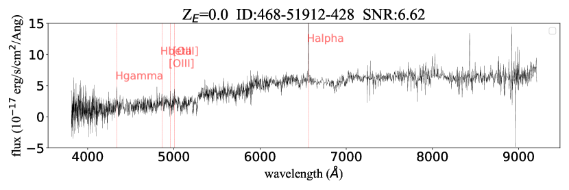
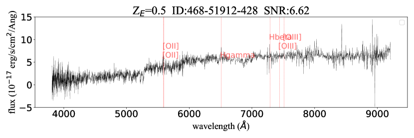
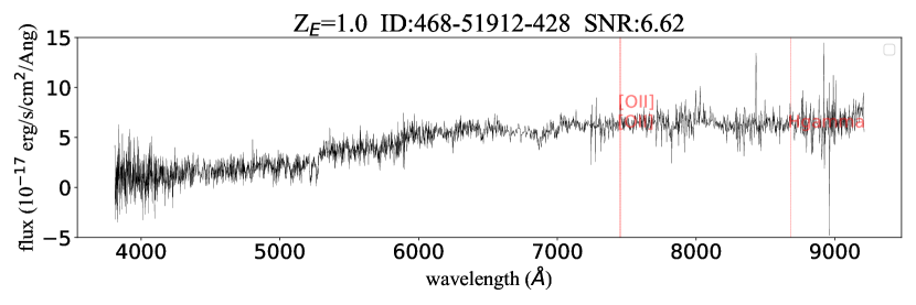
Figure 6: The spectra after adding artificial emission lines. We add the mock emission lines in several different redshift positions ($z_{E}$) in the real spectrum, in order to simulate the positive sample.

Simulated lines are first randomly generated at $z_{E}$=0 and then randomly redshifted to $z_{E}>z_{G}+0.1$, where $z_{G}$ is the redshift of the negative spectrum from which the positive is generated (see §3.4).

The flux at the redshift $z_{E}$ is then defined according to the standard equation:

$$F_{z_{E}}(\lambda)=F\left(\frac{\lambda}{1+z_{E}}\right)$$ (4)

where the function $F$ is the rest frame emission line flux function (Eq. 2).

The central wavelength of $F_{Z}$, $\lambda_{cz}$, is defined as

$$\frac{\lambda_{cz}}{1+z_{E}}=\lambda_{c0}\ \to\ \lambda_{cz}=(1+z_{E})\lambda_{c0}.$$ (5)

The interval of $\lambda$ is equal

$$\frac{\mathrm{d}\lambda^{\prime}}{1+z_{E}}=\mathrm{d}\lambda\ \to\ \mathrm{d}\lambda^{\prime}=(1+z_{E})\mathrm{d}\lambda$$ (6)

where $\lambda_{c0}$ is the central wavelength of the rest frame. According to the equations above, $\lambda_{c0}$ shifted to $(1+z_{E})\lambda_{c0}$, and the interval of $\lambda$ in the rest frame will broaden to $(1+z_{E})\mathrm{d}\lambda$.

Figs. 4 and 5 show how typical simulated emission lines from Table 2 are simulated according to the random parameters from Eqs. 3 and shifted to 0.5 and 1 redshifts.

3.4 Simulating the positive sample

The next step is to build a positive sample by adding simulated emission lines to the negative sample. As anticipated, we use the same lines as in Table 2, this time with lines redshifted to $z_{E}>z_{G}+0.1$, with the condition that $z_{E}\mathrel{\hbox to0.0pt{\lower 3.5pt\hbox{\hskip 0.5pt$\sim$}\hss}\raise 0.5pt\hbox{$<$}}1.2$.

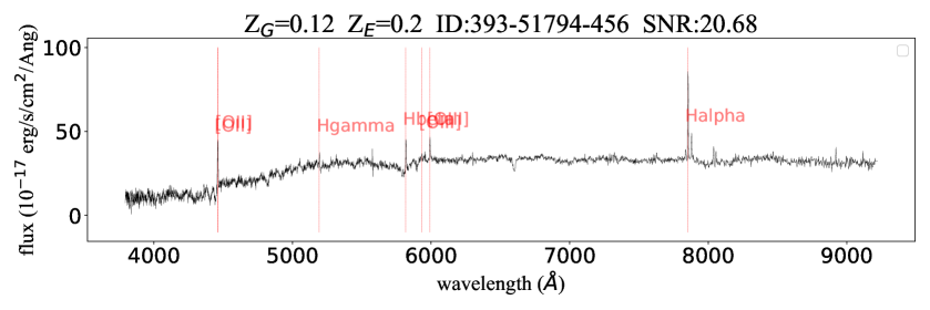
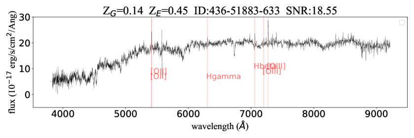
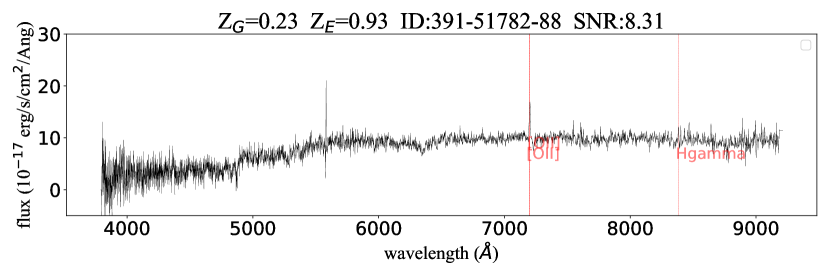
Figure 7: Spectra of confirmed gravitational lenses in Bolton et al. (2008), the red line is the location of the identified emission lines.

In Fig. 6 we show three simulated positive spectra for a single moderate SNR ($\sim 7$) negative spectrum (SDSS-468-51912). Here, we have marked the location of the simulated emission lines at different redshifts, on top of the continuum of the real eBOSS galaxy spectrum. Looking at these spectra, one can visually figure out what are the major challenges to identify the “ground truth” emission lines in them. First, the SNR of the lines, as this depends not only on the $h_{1}$ and $h_{2}$ but also on the intrinsic spectrum noise. Second, the contamination from residual sky lines, e.g. at $\lambda>8000$ Å. Third, the effect of the source redshift, which can shift most of the relevant emission lines from Table 2 out of the spectral range (at $\lambda>9200$Å, e.g. in Fig. 6-c). This latter issue could be in principle solved by including more emission lines in our reference catalog. We will consider this option for the next developments of GaSNets. However, we stress here that adding more lines, which in most of the cases have much lower SNRs in real galaxies, might introduce more uncertainties in the predictions of the GaSNet-L2, as they might be easier confused with random noise, especially in low-SNR spectra.

As a comparison with real lensing events, in Fig. 7 we report some spectra of confirmed lenses from Bolton et al. (2008, see also §3.5). Here the locations of the emission lines of the background sources are marked, again, as red vertical lines. In particular, in this figure, we show spectra with different SNRs to visualize the impact of the spectra quality on the recognisability of the lines. In SDSS-393-51794 all lines are visible and show a pattern similar to the simulated lines in Fig. 5. In SDSS-436-51883, despite the spectrum’s SNR being comparable to the one above, the lower signal of the background lines makes some of them embedded in the noise, although some others still stick out rather clearly. Here, the number of visible lines is reduced by the higher redshift of the source ($z_{E}=0.452$). Finally, in SDSS-391-51782, the redshift of the source ($z_{E}=0.931$) permits the observations of only two lines, which are yet rather easy to spot because of the decent SNR of the spectrum and the high signal of the lines. Overall, these examples show the kind of features the CNN needs to be trained on identifying in the spectra and the impact of the spectra quality and SNR of the background emission on the final line detection and redshift determination.

Similarly, these examples provide textbook cases of HQ candidates we will visually grade among the high probability candidates provided from the GaSNets (see §5.2).

3.5 Confirmed lenses from previous spectroscopic searches

As anticipated in the previous section, we also collect candidate/confirmed lenses from previous spectroscopic searches in SDSS/BOSS, using standard techniques, to be used as a real test sample for our deep learning tools. In particular, we have collected 131 objects from Bolton et al. (2008), 45 from Brownstein et al. (2012), and 118 from Shu et al. (2017), that have secure confirmation based on HST follow-up. This “test sample” made of real systems is useful for two main purposes: 1) to measure the completeness of our tool, by checking how many of these lenses are recovered by GaSNet-L1; 2) to test how accurate the GaSNet-L2 and GaSNet-L3 are in determining the $z_{E}$ and $z_{G}$, respectively. We will also compare our final catalog of HQ candidates vs. the latest highly complete sample of spectroscopic selected candidates in eBOSS from T+21. This will allow us to check the presence of candidates missed by standard techniques, and compare the different approaches.

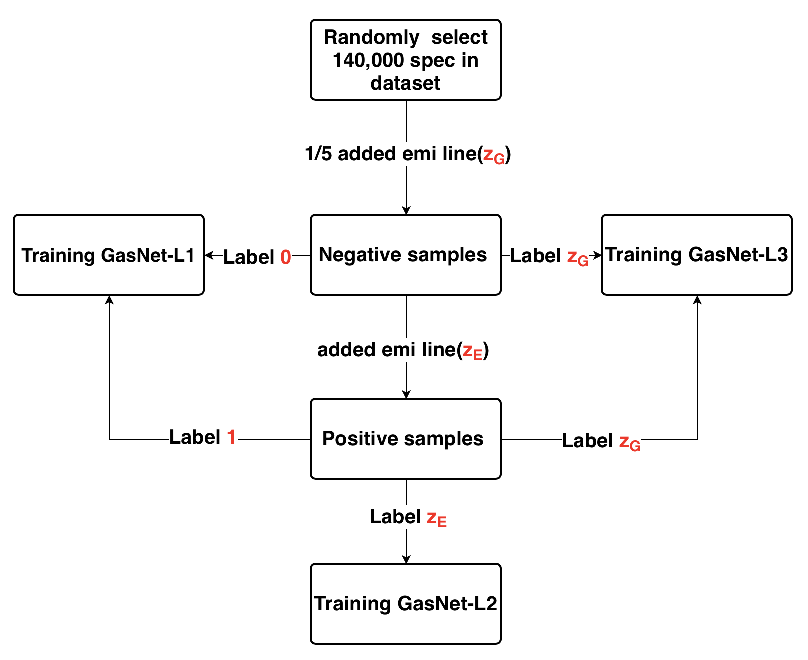
Figure 8: Summary of the training data building process. After constructing the negative and positive samples, they are labeled before they are fed into the training process of the three GaSNets. In this scheme, we illustrate the steps made to add the label to the two training samples.

4 Implementation

To proceed with the construction of the training and test samples, we collect 140 000 positives and the same number of negatives. These samples are further split into the 3 datasets: 100 000 for training, 20 000 for validation, and 20 000 for testing. The first two samples are used to train the GaSNets and evaluate how well the model predicts the ground truth targets based on the unseen data during the training process. The last sample is used to qualify the final performance of the GaSNets. Finally, we also test the performance against real candidates from literature, as discussed in §3.5.

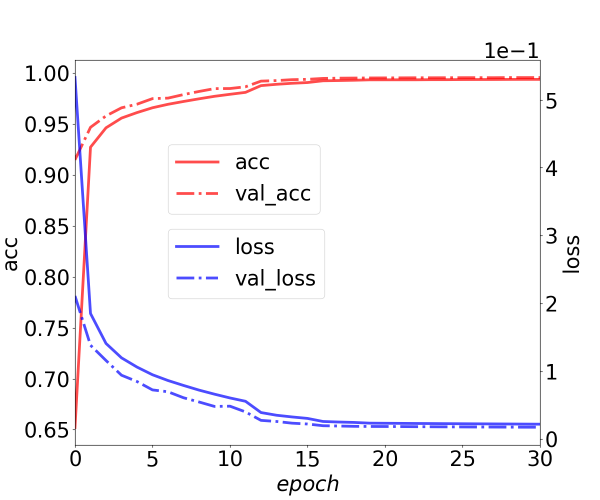
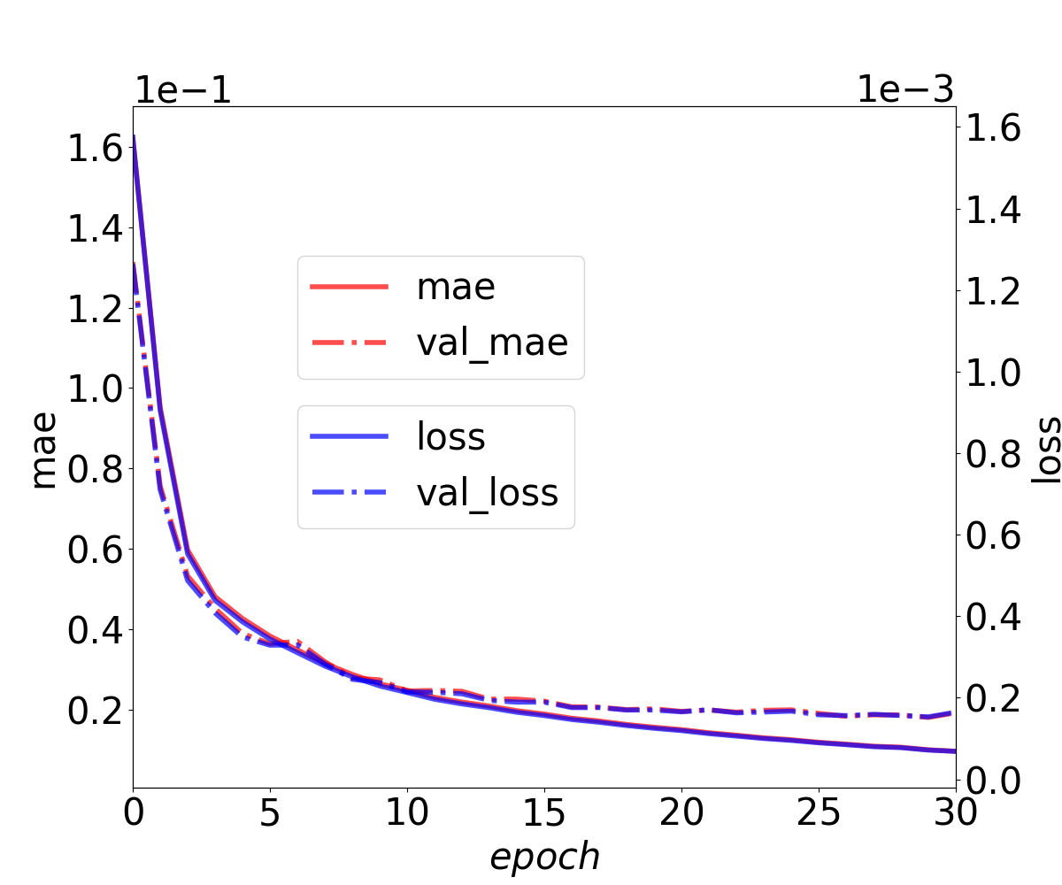
Figure 9: GasNets training results. Left panel: accuracy and the loss of GasNets-L1, the training and evaluation curves both converge to the same point, and show high accuracy. Middle panel: MAE and loss of GasNets-L2, which show a worse but yet acceptable convergence, with a reasonably low MAE. Right panel: MAE and loss of GasNets-L2, which well converge to the same values, because $z_{G}$ is easier to predict than $z_{E}$.

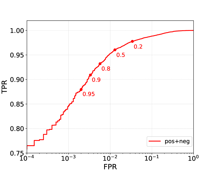
Figure 10: ROC curve of training samples where the true-positive rate (TPR) is plotted against the false-positive rate (FPR) (see text for details).

4.1 Training the Networks

According to the description in §2.3 and the tasks they are expected to fulfill, during the training, the GaSNets are fed with the training spectra to produce accurate predictions of the “target” quantities. For GaSNet-L1  the inputs are the spectra of the positives and negatives as well as their labels to give as output the probabilities ($P_{L}$) to be lens candidates. For GaSNet-L2, the inputs are the simulated positive spectra with their labels, while the outputs are the predicted redshifts of the emission lines $z_{E}$. For GaSNet-L3, the inputs are the labeled spectra of positives and negatives and the output are the redshifts of the foreground spectra ($z_{G}$). The full process of the training sample building and labeling is summarized in Fig. 8.

Table 3: Statistical properties of the predicted parameters

Sample	var.	$R^{2}$	Out. fract.	NMAD	MAE	MSE
Test	$z_{PE}$	$0.941$	$0.0121$	$0.0029$	$0.0164$	$0.0032$
Test	$z_{PG}$	$0.998$	$0.0003$	$0.0009$	$0.0017$	$0.0001$
Real	$z_{PE}$	$0.770$	$0.0840$	$0.0062$	$0.0535$	$0.0173$
Real	$z_{PG}$	$0.989$	$0.0047$	$0.0012$	$0.0033$	$0.0004$
All	$z_{PG}$	$0.988$	$0.0012$	$0.0009$	$0.0020$	$0.0002$

Regarding the training step, for GaSNet-L1 and GaSNet-L3 we use the 120 000 positive (traning+validation data) and 120 000 negative samples, i.e. a total of 240 000 spectra. Since GaSNet-L2 only predicts the $z_{E}$, in this case the training+validation sample is made by 120 000 spectra from the positive sample only. For each GaSNet, we use the training data to train 30 epochs with a learning rate of 0.0001 and use validation data to evaluate the performance. We have found that this produces rather stable validation results. During the training process, we optimize the 3 GaSNets with the Adam optimizer (Friedman 1999).

4.2 Testing on simulation data

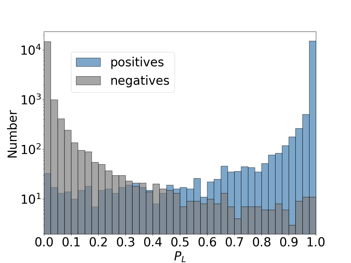
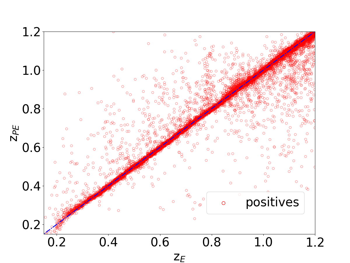
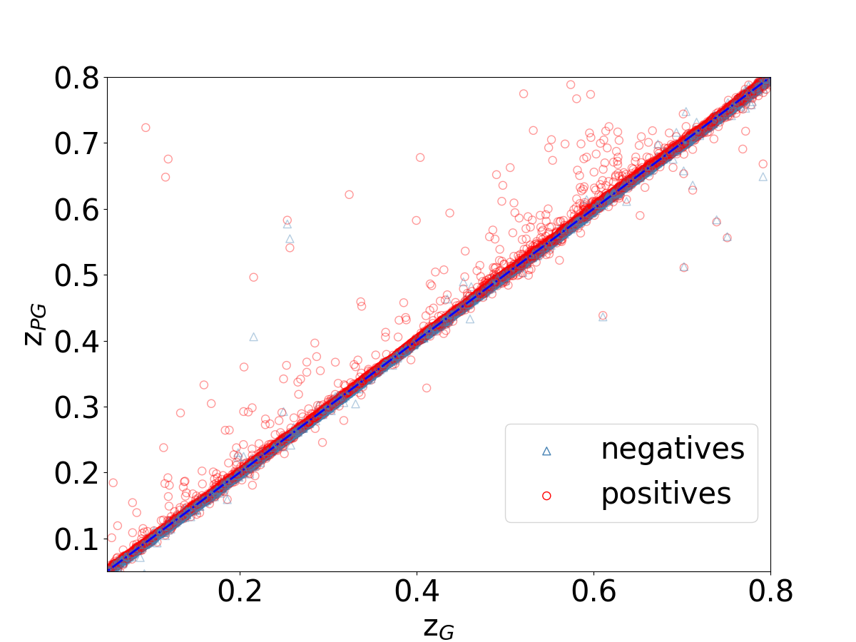
Figure 11: GaSNets results on the test sample. Left: the $P_{L}$ distribution from GaSNet-L1; Center: predicted emission line redshifts from GaSNet-L2, $z_{PE}$, vs. ground truth values, $z_{E}$; Right: predicted lens galaxy redshifts from GaSNet-L3, $z_{PG}$, vs. ground truth values, $z_{G}$.

After training, we first test the GaSNets’ performances using the simulated “test” spectra. As anticipated, the test sample is made of 20 000 positive and 20 000 negative samples for GaSNet-L1 and GaSNet-L3 and 20 000 positive samples for GaSNet-L2 .

In Fig. 9 we first show the results of the training run for the three GaSNets to have a first evaluation of their performances. In particular, we plot the first 30 training epochs. The solid lines in Fig. 9 represent the accuracy reached on the training data as the average deviation of the predictions from the ground truth (loss). The dot-dashed lines represent the same quantity on the test data.

For each GaSNet, we set a different evaluation function: for GaSNet-L1, being a classifier giving a probability as output, we use the “accuracy” (acc) as loss variable; for GaSNet-L2 and GaSNet-L3  as they predict the $z_{E}$ and $z_{G}$, we set the mean absolute error (MAE) as loss variable. From Fig. 9, GaSNet-L1 and GaSNet-L3 both show good convergence at about the same epoch toward the end of the training, while GaSNet-L2 shows a larger loss because of the degeneracy between noise and emission lines (see comment above). One possibility to improve this result might be the adoption of some spectra pre-processing, e.g. via smoothing. However, this would imply an incursion on the data characterization that is beyond the purposes of this paper, and we rather plan to address this in next analyses. Here, we just stress that the accuracy reached by GaSNet-L2 is high enough to separate the background emission lines from the foreground spectral features in lens candidates, hence more than sufficient for its actual purposes (see also §6.2).

In Table 3, we report some statistical estimators to measure the GaSNets’ performances. Besides the standard MAE and MSE, we add other three estimators.

First, the R-squared ($R^{2}$) is used to evaluate the linear relationship between prediction and true values. It is defined as

$$R^{2}=1-\frac{\sum_{i}(z_{P}-z_{T})^{2}}{\sum_{i}(z_{T}-\bar{z_{T}})^{2}}$$

where $z_{P}$ is the predicted value and $z_{T}$ is the true value, and $\bar{z_{T}}$ is the average value of $z_{T}$. The closer the $R^{2}$ is to 1, the better the prediction. In Table 3 we see that for the test sample, $R^{2}$ is close to 1 for both $z_{PG}$ and $z_{PE}$, meaning that both GaSNet-L2 and GaSNet-L3 are expected to produce accurate results.

Second, the outlier fraction, which is defined as the fraction of predicted redshifts scattering more than 15% from the true values:

$$\delta Z=\frac{\left|z_{P}-z_{T}\right|}{1+z_{T}}>0.15.$$

For the test sample, in Table 3 we show that the outlier fractions are $\mathrel{\hbox to0.0pt{\lower 3.5pt\hbox{\hskip 0.5pt$\sim$}\hss}\raise 0.5pt\hbox{$<$}}1\%$, implying a very small fraction of anomalous predictions.

Third, the normalized median absolute deviation (NMAD), which is defined as:

$$NMAD=1.4826\times median(\left|\delta Z-median(\delta Z)\right|).$$

It gives the absolute deviation of the predicted value from the central value of $\delta Z$. As seen in Table 3, the NMAD for the test sample is close to zero, meaning again a very small deviation from the true values, i.e. very accurate predictions.

In Fig. 10 we also show the receiver operating characteristic (ROC) curve where we plot the true-positive rate (TPR) against the false-positive rate (FPR). The TPR is the fraction of lenses that are correctly classified with respect to the total number of “ground truth” lenses, while the FPR is the fraction of non-lenses that are misclassified as lenses with respect to the total number of non-lenses. The ROC curve can be used to decide the probability threshold to adopt as a trade-off between true detection and contaminants from false positives. In the same figure, we report the TPR-FPR for different $P_{L}$s. We can see that for a $P_{L}=0.95$, we almost reach 90% completeness with a negligible false positive rate. We stress here that this result derived from simulated spectra is in rather ideal conditions. Hence, both the TPR and, most of all, the FPR might be just an upper and lower limit, respectively, as compared to the real cases. However, the $P_{L}=0.95$ occurs before the slope of the ROC becomes flatter, meaning that the gain in the number of true detections, at lower thresholds, increases at the cost of a larger number of contaminants. We will come back to these results later when we will discuss the threshold to adopt to select HQ candidates in real data.

Finally, in Fig. 11 we detail the results obtained for the test sample. On the left panel, we show the distribution of the $P_{L}$ from GaSNet-L1 for both the negative and the positive samples. As expected the former tends to cluster more toward a peak at $P_{L}=1$, but with a rather long tail toward the $P_{L}=0$, meaning that, statistically, there is a significant fraction of true positives to which GaSNet-L1 has given a low probability. We have checked these latter cases and found no correlation with the overall SNR of the spectra. Instead, we have found a correlation of the low $P_{L}$ objects with the $z_{E}$, in the sense that the larger the $z_{E}$, the bigger the number of the object with $P_{L}<0.5$. This suggests that either the lower number of lines or the intrinsically lower SNR of the lines suppress the $P_{L}$ and makes the classification of the lensing event more difficult at higher-$z$.

In the central panel of the same figure, we show the output of the GaSNet-L2 by comparing the predicted $z_{PE}$, against the ground truth values, $z_{E}$. Overall, the majority of the predicted values are tightly distributed around the one-to-one relation, as also quantified by the large $R^{2}$ values found in Table 3 (Test/$z_{PE}$). Numerous predictions scatter quite largely from the perfect correlation, because of the degeneracy of noise and background emission lines, as mentioned above. However, these are statistically irrelevant as the estimated outlier fraction in Table 3 is close to 1%.

Finally, in the right panel of Fig. 11, we show the predicted $z_{PG}$ from GaSNet-L3 against the ground truth values, $z_{G}$. In this case, the correlation is quite perfect and the outlier fraction is negligible ($<0.1\%$ see Table 3 – Test/$z_{PG}$), both for the positive and the negative sample. Indeed, for this latter test, we have also input the negative sample to check the performance of GaSNet-L3, as a pure automatic spectroscopic redshift tool, in absence of artificial emission lines. This shows that the ability of GaSNet-L3 to predict the galaxy redshift is not driven by the emission lines, easier to spot, but by the overall features of the spectrum (i.e. continuum and absorption/emission lines).

4.3 Test on HST confirmed samples

Previous analyses of the SDSS/BOSS spectra have brought to the collection of 294 strong lenses candidates: 131 from SLACS, 45 from BELLS, and 118 from S4TM (see §1). Being candidates based on spectroscopic features, these samples contain both real lenses and contaminants. Indeed, space imaging follow-ups have confirmed 70/131 SLACS candidates (the Grade-A objects in Table 4 of Bolton et al. 2008), 25/45 BELLS candidates (Grade-A objects in Table 3 of Brownstein et al. 2012), and 40/118 S4TM (Grade-A in Table 1 of Shu et al. 2017). As also commented in §1 these correspond to an average confirmation rate of 46%. Note, though, that the HST samples often tend to optimize the confirmation rate by pre-selecting targets with low-resolution imaging (see e.g. Bolton et al. 2004; Shu et al. 2016a), hence this can be considered an optimistic upper limit estimate. These are the main statistical samples that have been systematically followed up to collect space imaging confirmations of spectroscopically selected SGL candidates, using optical lines. As such, these represent the most secure sample to check our results against. These data can be used for two main purposes: 1) to compare the classification of the GaSNets against human selection and help us set a reasonable threshold to optimize the chance of finding real lenses with the minimal contamination from false positives; 2) to forecast the success rate we might expect from our set-up since we have a reference sample of “candidates” and “confirmed” events. Being this literature sample far from complete (see §2.1), it cannot be fully used to draw firm conclusions about the completeness of the GaSNets, however, this is the only sample we can use to benchmark the GaSNets’ performances, with a necessary grain of salt. On the other hand, the large sample from T+21, having no space observations cannot be used for the same purpose as the ones above. As anticipated, we will use it for an a posteriori test to assess the differences (if any) between standard and deep learning approaches.

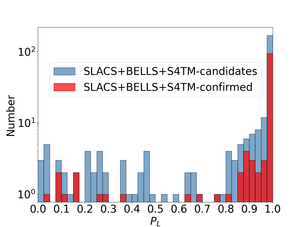
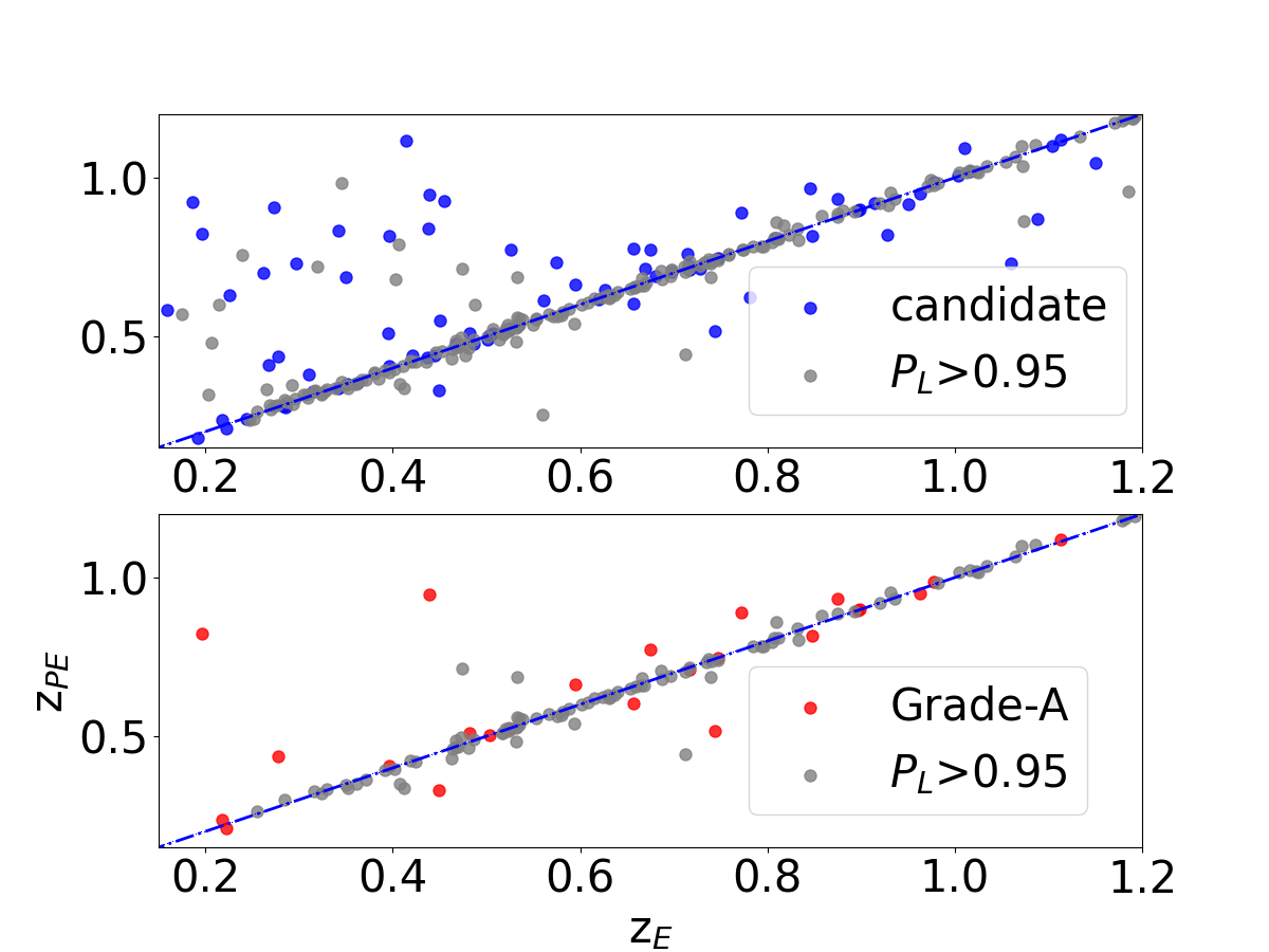
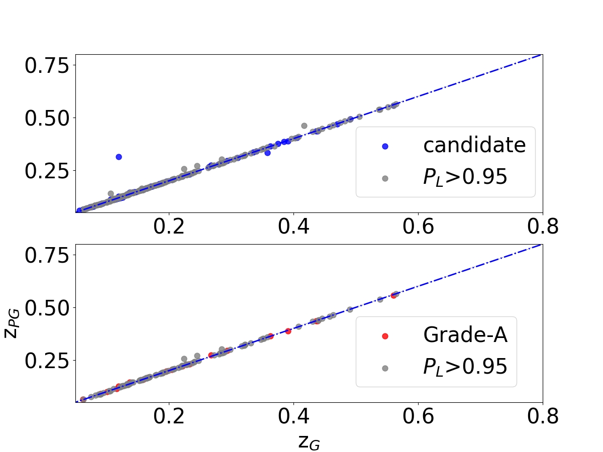
Figure 12: Results of the GaSNets applied to spectra of strong gravitational lens candidates (in blue) and HST-confirmed events (in red) from SLACS, BELLS, and S4TM samples (see text for details). Left: the $P_{L}$ distribution from GaSNet-L1; Center: predicted emission line redshifts from GaSNet-L2, $z_{PE}$, vs. literature redshifts, $z_{E}$, for the candidate objects (top) and the HST confirmed (bottom); Right: predicted lens redshifts from GaSNet-L3, $z_{PG}$, vs. literature redshifts, $z_{G}$, for the candidate objects (top) and the HST confirmed (bottom).

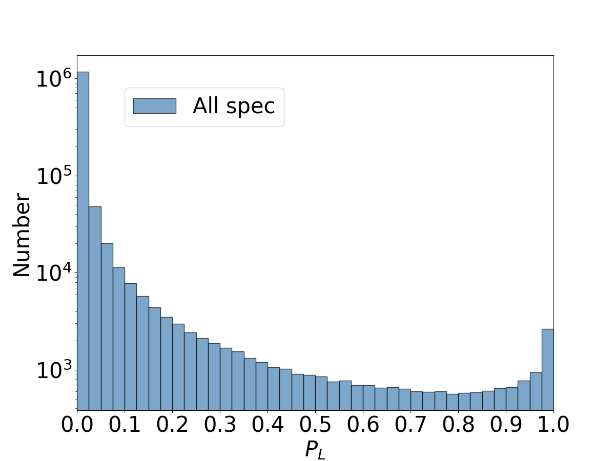
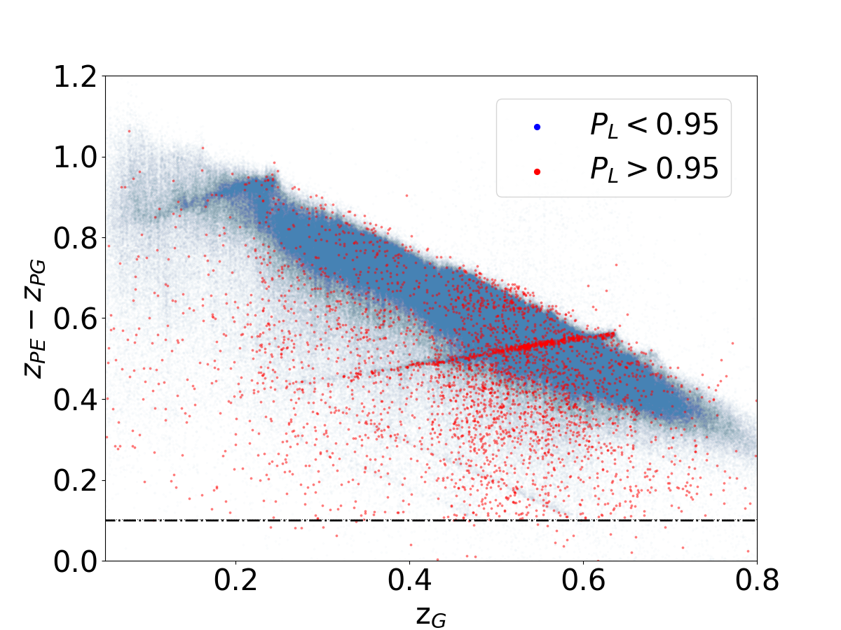
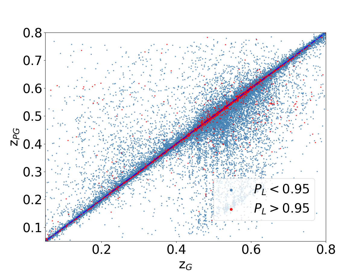
Figure 13: Predictions of the three GaSNets on the DR16-predictive sample ($\sim 1.3M$ objects): the $P_{L}$ from GaSNet-L1 (left), the $z_{PE}-z_{PG}$ (center) and the $z_{PG}$ (right), from GaSNet-L2 and GaSNet-L3 outputs, vs. $z_{G}$, the galaxy redshift from eBOSS/DR16 catalog (see text for the details). In the center and right panels we show the $P_{L}>0.95$ sample (in red) and the $P_{L}<0.95$ in blue.

To proceed with the test of the HST confirmed catalogs against GaSNets, we first select the literature spectra that are located in the predictive range of our CNNs (i.e. $0.05<z_{G}<0.8$ and $0.15<z_{E}<1.2$). These are 264/294 candidates and 121/135 confirmed objects. In Fig. 12 we show the probability predicted from the GaSNet-L1 (left panel), the redshift of the source predicted from GaSNet-L2 (central panel), and the redshift of the lens galaxies predicted by the GaSNet-L3 (right panel), for the candidates and confirmed literature objects face-to-face.

In particular, we see that GaSNet-L1 predicts high probabilities for most of the lenses: e.g., 69% of the candidates and 80% of the confirmed objects have $P_{L}>0.95$, which becomes 81% of the candidates and 90% of the confirmed objects for $P_{L}>0.8$.

More importantly, the ratio of the confirmed/candidates increases dramatically from $0.8<P_{L}<0.95$ to $P_{L}>0.95$, as we have 12/33, i.e. 36% for the former and 97/182, i.e. 53%, for the latter, vs. the overall 46% estimated for the full sample (see above). On the other hand, for $P_{L}<0.8$ the confirmation rate drops to 12/49, i.e. 24%, which is too low for successful space observations and still anti-economical for lens search in spectra. Indeed, as discussed in §4.2, at $P_{L}<0.8$ the FPR becomes prohibitive, producing massive false detections in large samples that should be cleaned with tedious visual inspections. Interestingly enough, for $P_{L}>0.95$ the fraction of true SGL events recovered (80%) is rather close to the TPR ($\sim 89\%$) predicted by the ROC curve (Fig. 10) for an idealized mock population of strong lenses. This means that the performances of the GaSNets on the real data might be not far from the expectations from simulated data.

However, In Fig. 12 (left) a misalignment between the deep learning and human filtered selections is further demonstrated by the fact that some confirmed lenses have received a small probability by GaSNet-L1. As discussed in the previous section, these are mainly low-SNR emission line spectra or higher-$z$ systems that, even if accounted for in the training sample, are difficult to be highly scored by GaSNet-L1 but might have been picked by the human eye with higher confidence. Hence, we conclude that a $P_{L}=0.95$ threshold is very likely to produce effective completeness higher than the 80% obtained above over a complete and unbiased true SGL sample.

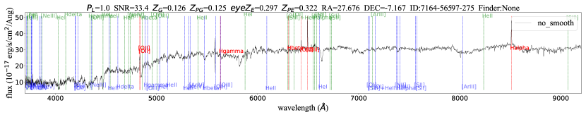
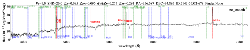
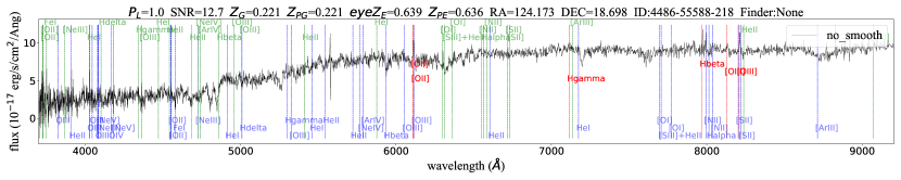
Figure 14: HQ candidate spectra. The SDSS/BOSS spectra are plotted with highlighted their main spectral features. Red vertical lines indicate the emission lines of the background source at the redshift $eyez_{E}$ (i.e. the one corrected during the visual inspection). Blue vertical lines indicate the spectral features of the lens at redshift $z_{G}$. Green lines show the location at rest frame ($z=0$) of the emission lines from sky). On the top of each spectrum from left to right, we report the probability from GaSNet-L1, the average SNR of the spectrum, the cataloged redshift of the galaxy from SDSS/BOSS, the predicted redshift from GaSNet-L3, the corrected redshift from visual inspection, the predicted redshift from GaSNet-L2, and finally, the RA, DEC, and ID of the target.

The middle and the right panel of Fig. 12 show that both GaSNet-L2 and GaSNet-L3 can make good predictions on the redshift of the emission lines and the lens galaxies. In general, GaSNet-L3 performs better than GaSNet-L2 (see Table 2), possibly because the spectra of the lens galaxies can provide more information, both from the continuum and the absorption or emission lines, while GaSNet-L2 relies only on a few emission lines, which provide intrinsically less information. We also see that the confirmed objects generally show a smaller scatter and outlier fraction than the candidates, especially in $z_{PE}$, and also that the highest probability objects show tighter one-to-one predictions. This demonstrates that misclassifications of SGL events might be related to uncertainties on the redshift of the background sources, which tend to be placed further away than sometimes they are, i.e. confusing “local” emissions with background ones. However, the chance of such misclassification is reduced for $P_{L}>0.95$ systems.

All in all, Fig. 12 indicates that the $P_{L}>0.95$ sample is accurate enough to produce reliable lens candidates from the DR16-predictive sample.

5 Results

In this section, we apply the trained GaSNets to the DR16-predictive sample, introduced in §3.1. This is made of 1 339 895 galaxy spectra and represents the sample among which we want to find new strong lens candidates and, for them, determine the redshift of the background source, $z_{E}$.

5.1 Predictions on the eBOSS spectra

According to the workflow described in Fig. 2, the first step to perform is the classification of candidates using GaSNet-L1. In Fig. 13 (left) we report the probability $P_{L}$ distribution obtained from GaSNet-L1 for the DR16-predictive sample. From this histogram, we see that using a $P_{L}>0.8$, which, according to the ROC curve, would return almost 95% of the true lenses, would produce a list of about 10 000 candidates. This is a sample hard to handle for two main reasons: 1) it is time-consuming to visually inspect and 2) it is foreseen to be severely contaminated from false detections. This latter case has been confirmed by randomly inspecting $100$ candidates with $0.8<P_{L}<0.95$ to find that about 90% are very poor candidates. On the other hand, choosing $P_{L}>0.95$, which, for the true lens cases, allowed to recover of $80\%$ of the confirmed lens known in SDSS/BOSS, would produce a more manageable sample of $\sim 4000$ candidates. Hence, at the cost of some acceptable incompleteness, for this first test, we decide to adopt a more conservative approach and search for high-quality candidates among the ones with $P_{L}>0.95$. We can now look into the predictions of the GaSNet-L2 and GaSNet-L3 to finalize the sample to visually inspect. In Fig. 13 (center) we report the redshift gap between the lens and the source, $\Delta Z=z_{PE}-z_{PG}$ as a function of the lens redshift $z_{G}$ for the full predictive sample. Here we highlight the objects with $P_{L}>0.95$, from all the other spectra in the predictive sample. We can distinguish a few features: 1) the upper limit imposed on the $z_{E}$ produces a zone of avoidance on the up-right side of the image; 2) there is a crowded sequence of high $P_{L}$ in the box defined by $z_{G}$=[0.5,0.6] and $\Delta z$=[0.4,0.6]. This is due to the presence of rather redundant residual emission lines from sky subtraction in the SDSS pipeline at $\lambda\sim 5600$Å (see Fig. 14) that is very often ignored by GaSNet-L2 but that in many cases is confused as a real emission. As we will see later, this sequence is easily filtered out by the visual inspection, but it has to be better accounted for in the training sample to reduce its impact in future analyses.

A similar effect is produced by the residual sky lines at $\lambda>8000$Å, which also produce a sequence of spurious $z_{E}$ predictions (see $z_{G}\sim 0.2$ and $\Delta Z\sim 0.9$). These have a small $P_{L}$, according to GaSNet-L1, and thus they do not bother, as they are excluded by the following analysis.

Overall, the $P_{L}>0.95$ sample looks rather unbiased, as seen by the $z_{G}$ estimates from GaSNet-L3 in the right panel of Fig. 13, where the predicted $z_{PG}$ is extremely tightly correlated to the eBOSS catalog values (see also the statistical estimators in Table 3).

However, before proceeding with the visual inspection of the background emissions estimated by the GaSNet-L2, to minimize the heterogeneity in the human grading, we pre-select the spectra that show an average SNR, computed at the expected positions of the reference lines from Table 2, $\langle$SNR${}_{\rm lines}\rangle$, to be larger than one. This further selection gives us 931 potential candidates pass to the visual inspection.

5.2 Visual inspection of spectra

The 931 candidates are visually inspected by the three authors, according to an ABCD ranking scheme, being A=“sure positive”, B=“maybe positive”, C=“maybe not a positive” and D=“sure negative”. To combine the human grading with the $P_{L}$, we have turned the ranking above into a score according to the conversion A=10, B=7, C=3, D=0 (see also Li+21). We finally select the spectra for which we have obtained an average score $\geq$7, as the final high-quality candidate sample. This is made of 497 objects in total.

Some spectra of this “high quality” sample are plotted in Fig. 14. Here we clearly see the emission lines, marked as red vertical lines, from background lensed star-forming galaxies.

During the visual inspection process, besides grading, we also check that the predicted values, $z_{PE}$ and $z_{PG}$, given by GaSNets, are perfectly aligned with visible spectral features. This is not often the case as the prediction process has some intrinsic uncertainty. For instance, the two GaSNets need to interpolate across a grid of training spectra that have been shifted with a coarse sampling (i.e. 0.05 in redshift, see Sect. 3.2). However, other sources of errors are possibly causing even more significant shifts, as we will discuss in more detail in Sect. 6.2. Using an interactive GUI developed by one of us (ZF), we then determine by eye the needed shift to obtain a perfect visual alignment and a “corrected” redshift for the $z_{PE}$, assuming the $z_{G}$ from the eBOSS catalog as an unbiased estimate of the main galaxy redshift.

Finally, to qualify a spectrum as a lensed galaxies candidate we check that 1) the emission lines do not belong to the sky lines (green lines in Fig. 14) and 2) that the identified emission lines, i.e. red lines in Fig. 14, having redshift $z_{PE}$ from GaSNet-L2, do not correspond to any line from the galaxy (i.e. blue lines in Fig. 14 at redshift $z_{PG}$ from GaSNet-L3). In other words, the $\Delta Z=z_{PE}-z_{PG}$ has to be larger than 0.1, as shown in Fig. 15, where it is plotted as a function of the estimated $z_{PG}$. Here we also see that the $\Delta z$ is decreasing with the $z_{PG}$ because the further the lenses, the smaller the difference in redshift with the background source. From Fig. 15 it is clear that this is mainly a selection effect due to our condition on the $z_{PE}<1.2$, however, since the high-quality candidates do not cluster toward the upper bound of the zone of avoidance, we conclude that the candidate distribution becomes incomplete when the $z_{PE}\sim 1.2$. This is consistent with the correlation of the low $P_{L}$ with the higher-$z_{PE}$ we have discussed in §4.2. An encouraging feature, in the same figure, is that the combination of the $\langle$SNR${}_{\rm lines}\rangle>1$ and the visual inspection, allows us to drop the stripe of spurious detection from residual sky lines discussed in §5.1.

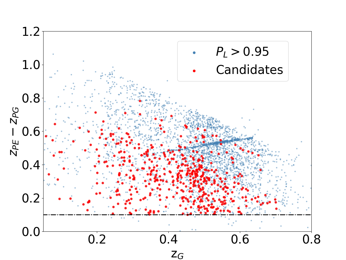
Figure 15: $z_{PE}-z_{PG}$ vs. $z_{PG}$ distribution of visual inspection 497 good potential candidates and all $P_{L}>0.95$ spectra

5.3 Deep learning vs. traditional methods

We end this section by comparing our HQ catalog, based on deep learning, with the catalog of 1551 candidates selected with the rest-frame optical bands from T+21, using traditional selection methods. They used the complete eBOSS/DR16 database and applied the standard spectroscopic detection method introduced in the eBOSS Emission-Line Lens Survey (BELLS) and added Gaussian fit information, grading, additional inspection observables, and additional inspection methods to improve the BELLS selection method. They used a total of 2 million objects with no selection on the redshift of the lenses. Furthermore, they used a larger database of reference lines, including also [NII]a/b and [SII]a/b: these are best suited for low-redshift detections being all placed at $\lambda>6500$Å, leaving the only [OII] doublet as a feature for the identification of background sources at $z\leavevmode\nobreak\ \hbox to0.0pt{$>$\hss}{\lower 4.30554pt\hbox{$\sim$}}1.2$. As such, their predictive sample is wider in the parameter space than the DR16-predictive we have adopted. For a proper comparison, we have selected the T+21 candidates that fall in the GaSNets predictive space (i.e. $z_{G}=0.05-0.8$, spectra SNR$>2$, $z_{E}\mathrel{\hbox to0.0pt{\lower 3.5pt\hbox{\hskip 0.5pt$\sim$}\hss}\raise 0.5pt\hbox{$<$}}1.2$, $z_{E}=z_{G}+0.1$) and finally obtain 778 “compatible” candidates ($\sim 50\%$ of the original sample). We have checked the excluded 773 and found that 739 detections are, indeed, based on a single line (generally in spectra with SNR$>2$) and 29/5 are based on 2/3 lines (all with spectra SNR$<2$), according to the T+21 catalog. Hence, the majority of these “known candidates” would have been missed anyways in our HQ catalog because of the conservative selection in the number of lines to use for the classification, either in the deep learning training or visual ranking.

We have, then, matched the compatible 778 candidates with our HQ sample of 497 entries and, surprisingly, we have found a match for only 68 objects.

The positive note is that GaSNets have found $\sim 430$ new HQ candidates that have been missed by standard techniques. The negative note is that the GaSNets seem to have missed $710$ candidates from T+21.

Is this true? To answer this question we need to first check how many of these objects are lost by the GaSNets according to the criteria imposed on their outputs, i.e. they do not fall in the criteria $P_{L}>0.95$ and $z_{E}-z_{G}>0.1$. These are 327, i.e. $42\%$ of the compatible sample. This is larger than the fraction of lost objects found in the test against the real systems in §4.3 (i.e. $100-69=31$% of “candidates” and $100-80=20$% confirmed ones, having $P_{L}<0.95$). One explanation of this excess of lost objects with low $P_{L}$ can be that these are mainly optimistic candidates in T+21, for which the GaSNets have given low reliability. To confirm this we have checked that 215/327 are single line detections, according to T+21, and only 87/327 have scored A+ or A in their check against low-resolution imaging. Hence, we can fairly conclude that this sample of lost candidates is overall low-valuable, having a tiny (albeit insecure) confirmation rate. This also implies that the fraction of lost SGL “real” events in our catalog is in line with the one estimated in §4.3, reported above (i.e. 20%).

Going to the remaining lost candidates ($710-327=383$), in Fig. 16 we show the spectra (not line) SNR vs. the estimated redshift of the background lines from T+21, color-coded by the number of detected lines. From this figure, we observe that:

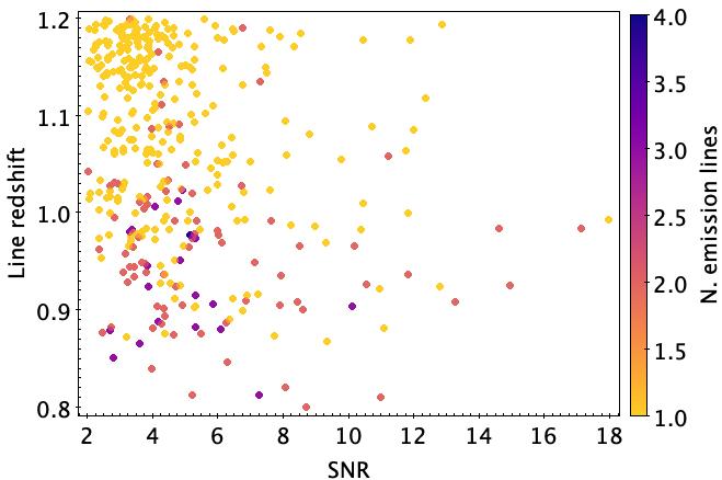
Figure 16: Sample of missing candidates in the HQ catalog from GaSNets+ visual inspection. In this figure, we show the distribution of the missing candidates in the parameter space adopted for the training of the GaSNets (i.e. spectra SNR$>2$ and $z_{E}<1.2$). Each candidate is color-coded by the number of detected lines in their spectra (according to T+21). Most of the missed candidates are 1-line and did not qualify in our HQ sample.

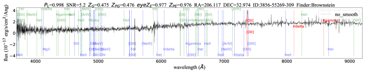
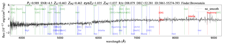
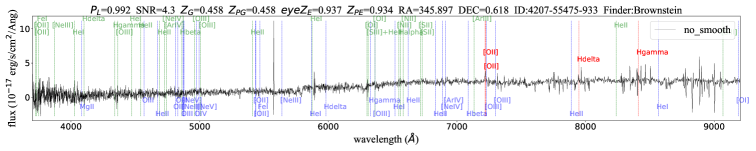
Figure 17: Sample of missing candidates in the HQ catalog from GaSNets + visual inspection and found in T+21. The red vertical lines are the features identified as multi-lines in T+21, but that have been excluded by us because either too faint or embedded in noisy regions, making them poorly reliable to qualify as HQ candidates.

1) The majority (286/383, i.e. 75%) of the missing candidates have 1-line detection, thus they are lost from our HQ catalog because we excluded them in our filtering (both because of the $\langle$SNR${}_{\rm lines}\rangle$ or the visual inspection, see §5.1 and 5.2). According to the T+21 low-resolution grading, 164/286 of the 1-line detections have A or A+ scores, which implies a rather large confirmation rate, $\sim$60%, if confirmed by higher-quality imaging. This is a sample we can easily intercept with GaSNets, by simply releasing the conservative criterion of the 1-line. From Fig. 16, we see that above $z\leavevmode\nobreak\ 1.05$ we lose some 2-line candidates, which supports further the conclusion in §5.2 that we are incomplete at $z_{E}\mathrel{\hbox to0.0pt{\lower 3.5pt\hbox{\hskip 0.5pt$\sim$}\hss}\raise 0.5pt\hbox{$<$}}1.2$.

2) The remaining 97 multi-line objects, in Fig. 16, majorly concern us, as according to their $P_{L}$ and number of lines should have been picked by the GaSNets + visual inspection. First, we have found 10/97 objects classified as quasar or unknown in DR16, so these could not be in our catalog. For all the other 87 we have visually inspected the spectra and found that despite they being classified as multi-lines in T+21, no line, except the [OII] doublet, had an acceptable SNR. Hence, these are all candidates that have been substantially treated as 1-line from us or given a rather poor visual grade. We give some examples of these spectra in Fig. 17. Since 60/97 have received A or A+ scores from the low-resolution confirmation in T+21, i.e. 60%, this is a sample that is likely to be valuable and should not be missed. However, we need to point out that this sample was not lost by the GaSNets but by human selection.

5.4 First catalog of new HQ strong lensing candidates in eBOSS from Deep Learning

After having subtracted the 68 candidates already found in T+21, we obtain a final catalog of 429 new HQ candidates in eBOSS, the first fully derived using deep learning. The full catalog is reported in Appendix A. This includes information about 1) RA/DEC coordinates; 2) plate ID; 3) MJD (Modified Julian Day), the observation date; 4) the GaSNet-L1 probability, $P_{L}$; 5) the redshift of the galaxy from the eBOSS catalog; 6) the predicted redshift of the galaxy from GaSNet-L3; 7) the predicted redshift of the background source from GaSNet-L2; 8) the corrected redshift of the source from the visual inspection (see Sect. 6.2); the total probability, $P_{T}=P_{L}\times 0.1$ visual scores, i.e. combining the GaSNets and human probabilities to be a lens.

6 Discussion

In the previous section, we have presented the final list of 429 new strong galaxy lensing candidates, obtained by applying the three GaSNets to the latest eBOSS database (DR16), and further cleaning the sample via visual inspection.

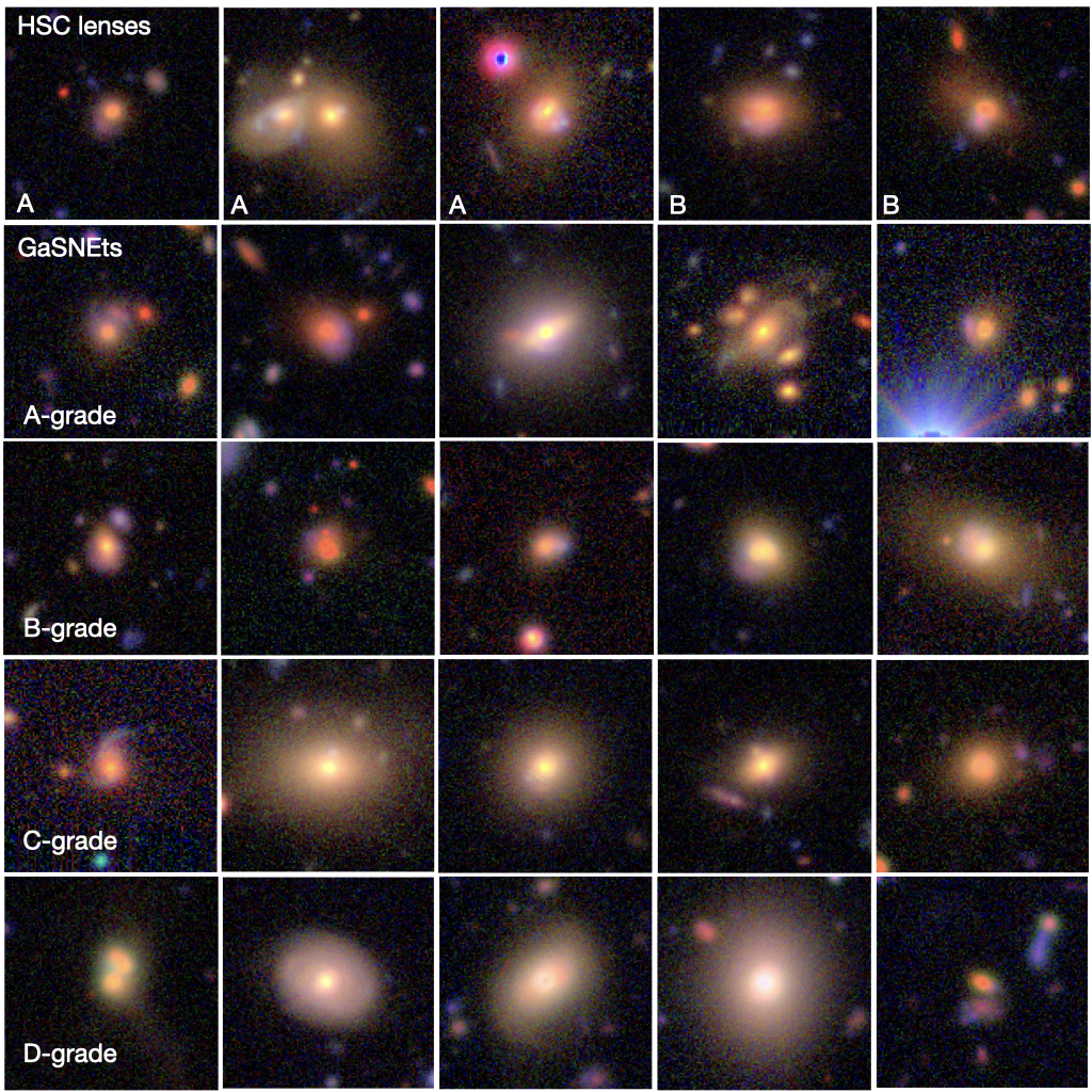
Figure 18: Some examples of ground-based color cutouts ($20^{\prime\prime}\times 20^{\prime\prime}$) of GaSNet candidates. Top row: match with HSC known candidates, re-graded as in the bottom-left corner. GaSNets have found them as HQ candidates independently. Bottom 4 rows: A, B, C and D ranked HSC counterparts of GaSNet candidates from the HQ sample in §5.4.

Strictly speaking, the GaSNets’ candidates consist of systems where, in the spectrum of a foreground galaxy, we have found emission lines that are incompatible with belonging to the same galaxy. We have assumed, so far, that all these lines come from lensing events. In reality, they can be emitted by other kinds of sources, like overlapping galaxies along the line of sight, outflows in late-type galaxies, interacting systems, etc., although we have set a redshift gap, $\Delta z$, that might have prevented the confusion with some “local” phenomena. Hence, to fully assess the new catalog, we need to estimate a fiducial confirmation rate based on space observations or high-quality ground-based imaging. Such a confirmation rate is important 1) to compare with the one from standard techniques, to see whether Deep Learning can outperform them in terms of reliability of the candidates; 2) to check whether the large spectroscopically selected samples accumulated so far, are compatible with expected numbers of SGL events from theoretical predictions (see e.g. 2.1), or we might expect to find more events with more refined tools.

Besides the confirmation rate, in this section, we also discuss the possibility to use the GaSNet-L2 and GaSNet-L3 as automatic tools for redshift estimates and spectra classification. We will conclude this discussion with some perspective on the next improvements of the GaSNets.

6.1 Confirmation rate via ground based imaging

To properly derive a fiducial confirmation rate for the 429 HQ candidates in §5.4, we have checked the HST archive observations to look for serendipitous matches with our newly discovered candidates but found no matches. Hence, the only remaining check we can perform is inside archive observations from the ground. There are three datasets potentially useful for the test: 1) DECaLS; 2) KiDS and 3) HSC. We have found 279 matches with DECaLS, 16 with KiDS, and 63 with HSC, however: 1) the quality of the DECaLS grz color images from the public data is rather poorer than other surveys and made the identification of the lensing features extremely uncertain (see Appendix B); 2) the number of KiDS matches is too small to have a fair statistics and we decided to leave the few convincing candidates for future analyses; 3) the HSC sample is the one with sufficient large statistics, image quality, and uniformity to make a fair estimate of the fraction of convincing lenses without strong biases.

Looking at this latter sample, we find that 7 candidates have corrupted color images or are too close to some bright source to be used with sufficient confidence. Hence, we finally inspect 56 systems. Of these, our HQ candidates match 8 known lens candidates from HSC (e.g., Sonnenfeld et al. 2018, 2019), although they are all C-graded by the imaging only in their catalogs. We have visually inspected them again and, applying the ABCD scheme as in §5.2 and taking into account the spectroscopic evidence, we have reclassified 3 of them with A-grade and 5 with B-grade.

Of the remaining 49 matches, we have classified 7 candidates as A-grade and 17 as B-grade systems. Taking the A-grade as bona fide confirmed lenses and weighting the B-grade ones by a 0.5 factor to account that they may be not lenses, we conclude that the lens confirmation rate is 21/56 or 38%, which is lower than the confirmation rate estimated in §4.3 using space imaging.

In Fig. 18 we show a gallery of the “confirmed” lens and, as a comparison, the “unconfirmed” ones (i.e. the ones C- and D-graded). In the first row, we report some of the lenses previously found in the HSC imaging and confirmed and re-graded by us, in the second and third rows some examples of new GaSNets’ confirmed lenses with A-grade, and B-grade, respectively. In the final two rows the unconfirmed C and D cases. These clearly show the variety of potential contaminants, including arc-like features of unclear nature, blue/faint background galaxies similar to other objects in the field-of-view, interacting systems, and large late-type or lenticular galaxies. In these latter examples, especially the large galaxies, if we exclude the cases where it is likely that the background emissions found in the spectra come from unlensed faint background systems as they can be seen in field-of-view, it is difficult to identify any other potential high-$z$ emitters. This leaves the nature of these emissions unresolved. In principle we cannot exclude that, given the small area covered by the fibers in eBOSS ($2^{\prime\prime}$, see also Fig. 18) there is some very low separation arc, embedded in the bright foreground galaxy light, remaining undetected in the seeing-confused images from HSC. In this case, we can argue that the confirmation rates estimated above (38%) might represent a lower limit.

If this conclusion is correct, we can attempt to derive a prediction of the total number of true SGL events in eBOSS, based on the current candidates from T+21 and this work. Put together they are 1551+429=1980. Assuming a pessimistic confirmation rate of 38%, they make $752$ real SGL events, while for a more optimistic $46\%$ conformation rate of SLACS+BELLS+S4TM, it makes $911$ real SGL. If we add the other candidates found in BOSS from BELLS (25) and BELLS GALLERY (17) we reach 794 and 953 real SGL, which nicely bracket the expected number we have estimated in §2.1 for BOSS ($\sim 920$). This suggests that we have possibly reached the full completeness of the lens population accessible by the largest spectroscopic database currently available.

6.2 Statistical errors of GaSNet-L2 and GaSNet-L3

GaSNet-L2 and GaSNet-L3 are two CNNs that can perform the generic task to estimate the redshift of given features in 1D spectra. As such, they can be applied to spectroscopic databases regardless of the specific task of looking for strong gravitational lenses.

Certainly, the search for lenses requires a much lower accuracy in the $z_{PG}$ and $z_{PE}$, because the only condition to ring the bell for potential events is $\Delta z=z_{PE}-z_{PG}>0.1$, which is rather higher than typical spectroscopic redshift errors based on the human measurements. However, this condition is physically meaningful if $\Delta z$ is larger than the combination of the typical errors on $z_{PE}$ from GaSNet-L2 and $z_{PG}$ from GaSNet-L3, which also include the uncertainties that a deep learning process might introduce (activation, loss, training, etc.).

Hence, if on one hand, the assessment of the “bias” and typical “statistical errors” of the two GaSNets (L2 and L3) is needed to validate the pre-condition for the HQ candidates, on the other hand, they can also quantify the accuracy of the individual CNN as “automatic tools” for redshift measurements. In this latter case, we can possibly require the typical errors to be of the order of $<1\%$, and systematics smaller than this precision. At the same time, we should expect a negligible fraction of outliers/catastrophic events.

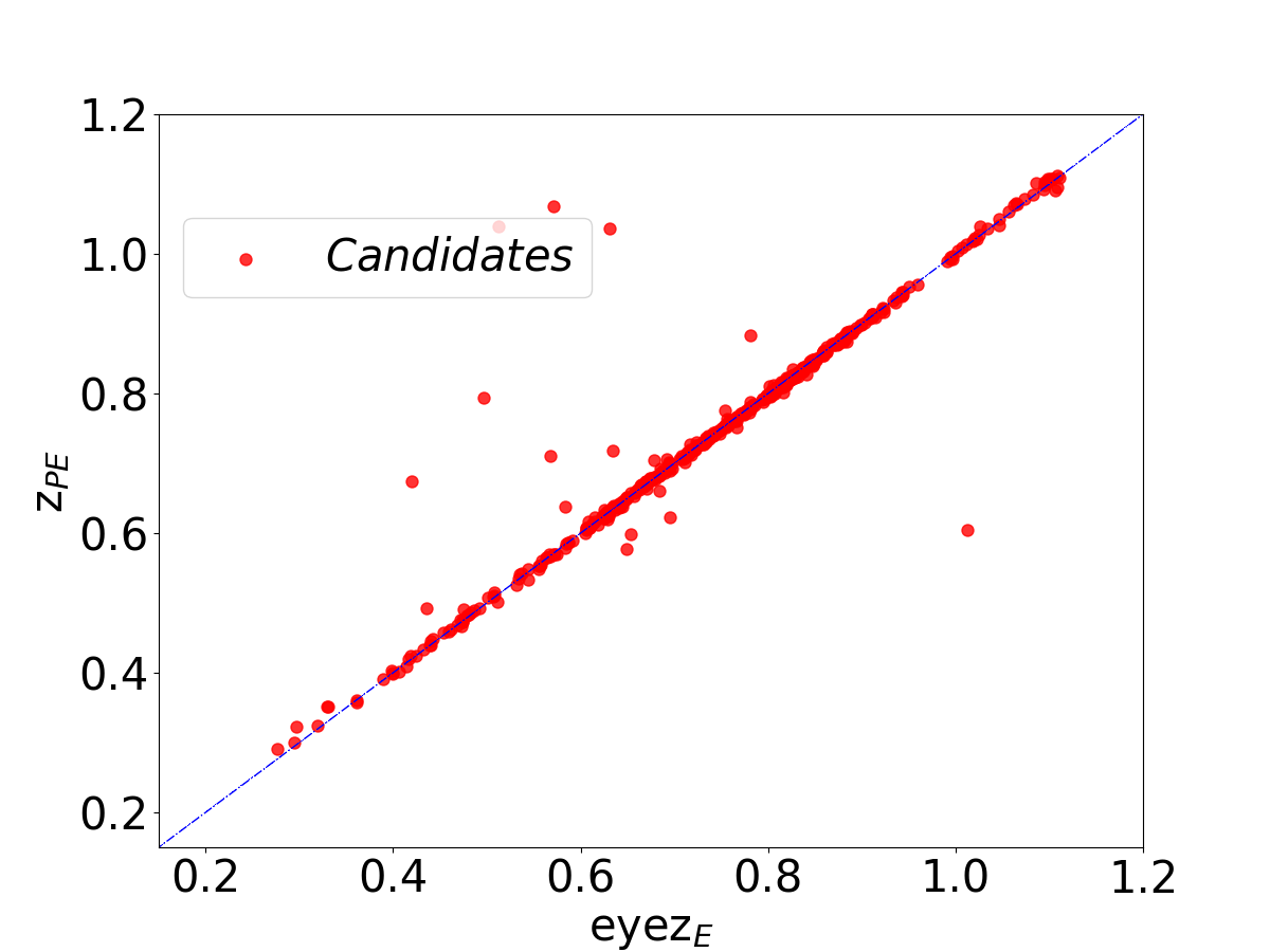
Figure 19: $Eyez_{E}$ vs. $z_{PE}$ and $eyez_{E}$, $z_{PE}$ distribution of visual inspected 429 HQ candidates.

As mentioned in §5.2, during the visual inspection we had the chance to check the accuracy of the $z_{PE}$ estimates and correct them by hand. This process is not error-free itself, as the resulting $eyez_{E}$ is a combination of a subjective identification of the line center and the accuracy in the line alignment by eye. However, we can confidently use these corrections, together with the nominal $z_{G}$ given in the SDSS catalogs, to compute the scatter of the GaSNet-L2 and GaSNet-L3 predictions and derive systematics and statistical errors for $z_{PE}$ and $z_{PG}$. For the $z_{PG}$ we can use all the galaxies in the predictive catalog as shown in Fig. 13 (right), for which $z_{G}$ is known, to determine the $\delta_{z_{PG}}=z_{PG}-z_{G}$. The scatter in this case is $\sigma(\delta_{z_{PG}})=0.015$. The outliers, defined as the spectra for which the $(|z_{PG}-z_{G}|)/(1+z_{G})>$0.15, are about 0.113%.

For the $z_{PE}$ we can use the spectra that we have visually inspected and for which we have collected the average $eyez_{E}$ estimated by the three of us. These are shown against the $z_{PE}$ in Fig. 19 and used to estimate the $\delta_{z_{PE}}=z_{PE}-eyez_{E}$. In this case, we have estimated the scatter $\sigma(\delta_{z_{PE}})=0.046$, while the outliers are about 1.21%.

In both cases, the scatter and accuracy are reasonably good, and so it is the outlier fraction. This result confirms that the adoption of the $\Delta z>0.1$ is conservative enough to account for the nominal statistical errors of the predicted redshifts. Furthermore, if we consider that the SNR is generally poor for the majority of the emission lines of the background galaxies, then we believe that both GaSNets (L2 and L3) are a very promising start and can be possibly be already used to automatically provide a first accurate guess of the redshift of galaxies in large surveys, while a more dedicate training would possibly improve the overall accuracy. We will dedicate future analyses to the GaSNets on this latter and more applications, including specialized tasks for spectra classification (e.g. starburst galaxies, active galactic nuclei, irregular systems, etc.).

Figure 20: A possible scheme for increasing the interplay between the three GaSNets. Here, we foresee input GaSNet-L1 with the outputs of GaSNet-L2 and -L3, as shown in the yellow line show, to improve the $P_{L}$.

6.3 Improvements of CNN model

In this work we have used 3 independent CNN models and combined their outputs according to some physically meaningful conditions (see Fig. 2), to identify strong lens candidates. In fact, because of the physics of the SGL, which involves the position of the source and lens with respect to the observer, the properties of the projected potential, etc., the 3 outputs of the GaSNets are not fully independent. Rather, they must be connected via the ray-tracing equation of the SGL. For instance, one can define a more meaningful probability for spectra to have caught a lens candidate, by looking at the relative distance of the $z_{PG}$ and $z_{PE}$, or at the absolute value of $z_{PG}$ (e.g. giving a lower $P_{L}$ if the galaxy is a very low redshift), etc. One possible future development is to connect different individual CNN networks (just like the neurons in our brain), for example, as in Fig. 20, to make a more educated probability for a spectrum to be an SGL system.

In this figure, we suggest using the prediction of $z_{PG}$ as conditional information for the prediction of $P_{L}$, then using the prediction of $z_{PG}$ and $P_{L}$ as auxiliary information for the prediction of $z_{E}$. If, on one hand, this architecture can help to improve the accuracy, the cost to pay is the model complexity, including a larger correlation among the different branches with some large back-propagation. This would make the overall model more time-consuming in terms of training and prediction, but likely more accurate and false detection free.

7 conclusions

In this paper, we have presented a novel deep learning tool to search for strong gravitational lensing (SGL) events in 1D galaxy spectra. This is the first attempt to use multiple emission lines after Li+19 used Ly$\alpha$ only.

The new algorithm is made of different CNNs, dubbed Galaxy Spectra convolutional neural Networks (GaSNets). These are optimized to work together to provide SGL candidates, but can also perform classification and regression tasks independently. As such, they are extremely suitable for further applications in large databases of tens to hundreds of millions of spectra, like the ones expected from the next generation spectroscopic surveys (4MOST, DESI, EUCLID, CSST).

In this paper, we have started by applying these new tools to the strong lensing search in the eBOSS/DR16 database (Ahumada et al. 2020). To this aim we have introduced: 1) GaSNet-L1 giving to each eBOSS spectrum the probability to be an SGL event ($P_{L}$); 2) GaSNet-L2 estimating the redshift of background sources ($z_{PE}$) from a series of pre-selected emission lines (see Table 2); and 3) GaSNet-L3 estimating the redshift of the galaxy itself ($z_{PG}$), using the information it learns from the continuous spectrum, including local absorption/emission features. Only working together, the three GaSNets efficiently pinpoint SGL candidates combining a high $P_{L}$ with the condition that the $z_{PE}>z_{PG}$, as expected for typical strong lensing configurations.

In particular, by testing the GaSNets on a list of known spectroscopically selected gravitational lenses in SDSS/BOSS (from Bolton et al. 2008, Brownstein et al. 2012, and Shu et al. 2017) we have found that using a $P_{L}>0.95$ we can recover about 80% of the strong lenses confirmed by HST. This very conservative probability threshold provided a reasonable trade-off between significant completeness and a reasonably small sample to visually inspect, with low contamination from false-positive detection.

Using this set-up, with the condition that $z_{PE}>z_{PG}+0.1$, we have applied the GaSNets to $\sim 1.3$ million spectra from the SDSS-DR16, after having imposed some appropriate cuts to guarantee a good spectrum quality and the visibility of at least two emission lines from the putative sources (namely, [OII] and $H_{\gamma}$), assumed to be star-forming galaxies.

We have collected $\sim 930$ candidates that have been further cleaned by misclassified SGL events, via visual inspection. The final sample of visual HQ candidates is made of 497 spectroscopic selected objects. This catalog has been a posteriori compared to the most extended catalog of spectroscopic selected lens candidates from T+21 and found an overlap of only 68 candidates, meaning that 429 of our candidates are newly found. On the other hand, we have demonstrated that GaSNets did not recover the remaining T+21 sample because of the conservative constraints we have adopted for the number of lines to be detected ($>2$). Releasing them, half of the sample from T+21 (i.e. the one for which GaSNets has $P_{L}>0.95$) remains under the GaSNets discovery reach.

For the new HQ catalog, we provide RA, DEC, the probability, $P_{L}$, the redshift of the galaxy from the eBOSS catalog, the predicted redshift of the galaxy from GaSNet-L3, the predicted redshift of the background source from GaSNet-L2, the corrected redshift of the source from the visual inspection, in Appendix A.

To estimate a tentative confirmation rate of these candidates, we have matched the coordinates with archive HST observations and found no matches. Instead, we have found optical counterparts in DECaLS, KiDS, and HST observations, but only HSC has provided sufficient statistics and image quality to confidently confirm the first sample of GaSNets’ candidates. Among these, we have independently confirmed 8 SGL candidates from previous HSC lens imaging searches, thus providing spectroscopic evidence of lensing events, even though for only 3 of them we have found convincing features in the imaging to be “sure lens”. Besides these “known” lenses, we have found a preliminary optical confirmation of a further 24 GaSNet HQ candidates, although, also in this case, for 17 of them the HSC images allowed only a “maybe lens” B-grade, and only 7 have a “sure lens” A-grade. Taking the A-grade as bona fide lenses and giving a 0.5 weight to the B-grade candidates, we have estimated a confirmation rate of $38\%$ for our HQ catalog.

Some examples of the HSC matched are shown in Fig. 18, where we also show low-graded imaging of GaSNet candidates. The possible contaminants are higher redshift galaxies, overlapping in the fiber spectra, or maybe local phenomena mimicking an SGL event. For example, local gas outflows, with typical velocities of $3\times 10^{3}$ kms^-1, will introduce asymmetric velocity distribution along the ejection direction (Veilleux et al. 2020), which would shift the wavelength of some characteristic emission lines. Among these the [OIII] line could deviate from the $z_{G}$ by $\sim 50$Å and produce a false positive.

In this paper, we have demonstrated that Deep Learning represents a very efficient method to search for strong lenses in galaxy spectra. This can be applied to next generation spectroscopic surveys in a fast and automated way. This first application to the eBOSS database has confirmed that the spectroscopic selection of SGL candidates is complementary to the imaging-based SGL searches. For instance, of the 32 A/B grade candidates from the GaSNets matching with HSC imaging, only 8 were found previously on HSC images. This over-performance of the spectroscopic searches with respect to imaging is particularly evident for ground-based observations, where the typical seeing has no impact on emission lines of background sources in spectra but makes it hard to resolve low-separation gravitational arcs of the same sources.

For this first application, we have made conservative choices regarding 1) the number of features to use for the training of the GaSNets; 2) the overall Network architecture, e.g. limiting the interconnections between the three GaSNets  3) the probability threshold to optimize the sample to visual inspect and keep the false positive under control. These are all directions to consider for future improvements. As a final positive note, we have discussed that the GaSNet-L3, in particular, has reached an accuracy and scatter of its predictions, sufficient to be used to automatically measure galaxy redshifts in large spectroscopic surveys.

Data Availability

The data that support the findings of this study are available at the URLs provided in the text and the Table in Appendix A. All other data that are not provided in the paper can be requested from the authors.

Appendix A HQ catalog from GaSNets

In this appendix we list the HQ candidates obtained with the GaSNets and described in §5. The table content is listed in §5.4.

New HQ candidates from GaSNets
	RA	DEC	PLATE	MJD	FIBER	$P_{L}$	z	$z_{PG}$	$z_{PE}$	$mean_{eyeZE}$	$P_{T}$
1	27.6755	-7.1667	7164	56597	275	1.0	0.126	0.125	0.322	0.297	1.0
2	356.6865	34.8954	7143	56572	678	1.0	0.095	0.096	0.291	0.276	1.0
3	124.173	18.6976	4486	55588	218	1.0	0.221	0.221	0.636	0.641	1.0
4	139.3617	31.157	5808	56325	434	1.0	0.239	0.238	0.823	0.82	1.0
5	205.2421	18.6312	5862	56045	110	1.0	0.244	0.244	0.638	0.645	1.0
6	233.5735	3.4663	4805	55715	326	1.0	0.291	0.288	0.707	0.708	1.0
7	22.0923	22.3834	5107	55940	409	1.0	0.277	0.275	0.7	0.695	1.0
8	356.4175	-2.1613	4356	55829	729	1.0	0.294	0.294	0.659	0.658	1.0
9	9.4789	17.8124	6193	56237	298	1.0	0.298	0.297	0.695	0.695	1.0
10	4.8287	26.2703	6276	56269	26	1.0	0.262	0.262	0.6	0.604	1.0
11	244.2444	59.9424	6976	56448	830	1.0	0.257	0.258	0.509	0.507	1.0
12	221.3814	60.9204	6982	56444	516	1.0	0.258	0.257	0.501	0.511	1.0
13	228.0721	14.4225	5486	56030	270	1.0	0.327	0.327	0.706	0.708	1.0
14	143.3092	22.088	5770	56014	842	1.0	0.35	0.35	0.694	0.694	1.0
15	352.9407	29.3635	6581	56540	976	1.0	0.313	0.312	0.68	0.678	1.0
16	202.7383	47.6651	6743	56385	86	1.0	0.349	0.35	0.662	0.662	1.0
17	145.3751	1.865	4736	55631	264	1.0	0.353	0.354	0.719	0.722	1.0
18	212.4583	58.3783	6804	56447	957	1.0	0.36	0.36	0.744	0.742	1.0
19	189.6944	51.0158	6674	56416	262	1.0	0.388	0.387	0.762	0.766	1.0
20	358.2568	32.3241	6498	56565	550	1.0	0.367	0.366	0.729	0.731	1.0
21	215.0974	30.7816	3866	55623	45	1.0	0.466	0.47	0.813	0.814	1.0
22	127.2466	6.7193	4866	55895	335	1.0	0.47	0.471	0.878	0.877	1.0
23	176.7038	31.9488	4614	55604	299	1.0	0.478	0.479	0.845	0.846	1.0
24	322.7388	-1.587	4384	56105	873	1.0	0.506	0.509	0.81	0.814	1.0
25	338.7334	15.1238	5038	56235	231	1.0	0.514	0.513	0.822	0.825	1.0
26	118.3424	11.0724	4511	55602	755	1.0	0.565	0.558	0.82	0.824	1.0
27	189.7042	24.9656	5984	56337	333	1.0	0.559	0.558	0.826	0.828	1.0
28	153.3944	25.7594	6465	56279	537	1.0	0.616	0.619	0.825	0.828	1.0
29	321.1025	1.1421	4193	55476	665	1.0	0.7	0.7	0.875	0.878	1.0
30	358.3876	-8.6495	7166	56602	784	1.0	0.167	0.167	0.653	0.657	1.0
31	253.2719	50.6749	6311	56447	56	1.0	0.095	0.093	0.57	0.575	1.0
32	321.5421	1.9777	5143	55828	640	1.0	0.152	0.151	0.772	0.78	1.0
33	150.7402	6.319	4874	55673	82	1.0	0.225	0.225	0.781	0.781	1.0
34	17.3453	18.7404	5124	55894	36	1.0	0.226	0.226	0.645	0.644	1.0
35	207.8211	-1.7923	4041	55361	522	1.0	0.208	0.208	0.77	0.774	1.0
36	31.4846	-2.3339	4347	55830	156	1.0	0.283	0.281	0.462	0.462	1.0
37	181.6564	37.855	4700	55709	242	1.0	0.263	0.262	0.607	0.609	1.0
38	26.7007	22.0027	5108	55888	811	1.0	0.267	0.266	0.745	0.745	1.0
39	128.9045	8.3751	5285	55946	510	1.0	0.259	0.258	0.555	0.558	1.0
40	42.3078	-2.8227	4342	55531	112	1.0	0.292	0.29	0.459	0.459	1.0
41	18.952	5.1636	4425	55864	376	1.0	0.337	0.336	0.607	0.606	1.0
42	173.7037	54.187	6697	56419	386	1.0	0.302	0.301	0.614	0.613	1.0
43	134.3035	19.7311	5175	55955	804	1.0	0.377	0.379	0.632	0.629	1.0
44	145.78	55.292	5710	56658	116	1.0	0.355	0.356	0.607	0.609	1.0
45	258.3841	42.9416	6062	56091	91	1.0	0.352	0.354	0.713	0.714	1.0
46	242.464	37.8714	5200	56091	151	1.0	0.448	0.448	0.648	0.648	1.0
47	176.8551	35.8301	4646	55622	879	1.0	0.473	0.473	0.658	0.658	1.0
48	199.5047	14.466	5425	56003	820	1.0	0.478	0.481	0.826	0.825	1.0
49	203.1219	19.9543	5861	56069	347	1.0	0.494	0.496	0.831	0.835	1.0
50	189.5541	23.2605	5983	56310	25	1.0	0.48	0.48	0.849	0.85	1.0

	RA	DEC	PLATE	MJD	FIBER	$P_{L}$	z	$z_{PG}$	$z_{PE}$	$mean_{eyeZE}$	$P_{T}$
51	248.9654	17.222	4064	55366	77	1.0	0.497	0.496	0.715	0.714	1.0
52	189.5441	46.0467	6635	56370	501	1.0	0.492	0.493	0.822	0.823	1.0
53	219.7836	54.8809	6710	56416	27	1.0	0.461	0.462	0.722	0.722	1.0
54	214.9087	19.692	5895	56046	973	1.0	0.528	0.527	0.883	0.883	1.0
55	331.1801	30.5522	5961	56460	545	1.0	0.538	0.552	0.83	0.832	1.0
56	6.3176	28.2843	6274	56550	455	1.0	0.501	0.502	0.816	0.816	1.0
57	240.6962	7.4048	4893	55709	858	1.0	0.622	0.623	0.869	0.874	1.0
58	115.6977	25.8798	4462	55600	271	1.0	0.441	0.441	0.682	0.684	1.0
59	160.3564	43.6801	4690	55653	424	1.0	0.238	0.236	0.439	0.439	1.0
60	180.9566	23.4359	5969	56069	846	1.0	0.263	0.263	0.612	0.619	1.0
61	177.6002	19.2965	5881	56038	604	1.0	0.289	0.288	0.476	0.474	1.0
62	139.0009	21.6609	5771	56011	574	1.0	0.322	0.322	0.511	0.508	1.0
63	30.0581	3.8889	4270	55511	7	1.0	0.429	0.427	0.776	0.754	1.0
64	133.0317	40.5817	4607	56248	711	1.0	0.447	0.446	0.842	0.844	1.0
65	129.9769	59.5436	5148	56220	583	1.0	0.475	0.474	0.821	0.822	1.0
66	164.8521	11.0051	5356	55979	881	1.0	0.473	0.473	0.832	0.834	1.0
67	189.5441	46.0467	6667	56412	1	1.0	0.491	0.493	0.822	0.822	1.0
68	154.1187	9.2856	5334	55928	953	1.0	0.545	0.544	0.859	0.86	1.0
69	354.6202	27.6904	6516	56571	543	1.0	0.549	0.547	0.846	0.848	1.0
70	118.5745	16.4872	4495	55566	811	1.0	0.607	0.607	0.812	0.814	1.0
71	152.2575	38.1894	4567	55589	235	1.0	0.648	0.648	0.828	0.828	1.0
72	337.6706	-1.1175	4203	55447	368	1.0	0.33	0.33	0.526	0.531	1.0
73	251.7678	29.8492	4189	55679	752	1.0	0.375	0.374	0.59	0.591	1.0
74	137.8548	16.6327	5301	55987	328	1.0	0.394	0.394	0.693	0.698	1.0
75	18.8537	-1.4834	4353	55532	663	1.0	0.438	0.438	0.802	0.805	1.0
76	144.1259	17.0156	5317	56000	579	1.0	0.403	0.404	0.819	0.821	1.0
77	6.512	9.7381	6195	56220	424	1.0	0.246	0.244	0.391	0.39	1.0
78	160.1055	3.5501	4773	55648	290	1.0	0.439	0.438	0.642	0.643	1.0
79	213.0731	46.9419	6751	56368	355	1.0	0.402	0.405	0.657	0.653	1.0
80	215.0974	30.7816	3867	55652	579	1.0	0.466	0.465	0.813	0.814	1.0
81	137.8928	43.2083	4687	56369	409	1.0	0.497	0.495	0.837	0.84	1.0
82	135.5464	1.2383	3816	55272	61	1.0	0.514	0.513	0.831	0.833	1.0
83	143.9865	53.3553	5724	56364	508	1.0	0.198	0.198	0.424	0.424	1.0
84	28.2369	-2.3081	4348	55559	155	1.0	0.534	0.536	0.669	0.665	1.0
85	350.6051	34.2495	7139	56568	687	1.0	0.292	0.29	0.612	0.612	1.0
86	224.9773	-2.6469	4020	55332	247	1.0	0.511	0.509	0.824	0.83	1.0
87	6.2129	-2.6018	4367	55566	263	1.0	0.583	0.584	0.85	0.852	1.0
88	156.6438	37.2146	4559	55597	409	1.0	0.484	0.484	0.636	0.639	1.0
89	185.1209	10.9196	5399	55956	433	1.0	0.507	0.507	0.707	0.712	1.0
90	140.0093	36.1607	4644	55922	855	1.0	0.595	0.594	0.882	0.883	1.0
91	201.2076	5.5061	4839	55703	339	1.0	0.58	0.581	1.018	1.018	1.0
92	184.1385	35.6992	4613	55591	234	0.999	0.347	0.347	0.728	0.73	1.0
93	22.0924	-3.7932	7047	56572	878	0.999	0.395	0.394	0.598	0.654	1.0
94	7.5599	24.7932	6281	56295	145	0.999	0.405	0.402	0.874	0.876	1.0
95	180.5188	55.022	6688	56412	521	0.999	0.512	0.512	0.83	0.832	1.0
96	9.2422	10.4302	5656	55940	264	0.999	0.178	0.178	0.357	0.361	1.0
97	336.5143	28.8703	6586	56485	471	0.999	0.507	0.502	0.825	0.829	1.0
98	39.6814	-5.6274	4399	55811	917	0.999	0.358	0.358	0.726	0.724	1.0
99	333.8121	13.4517	5041	55749	103	0.999	0.605	0.608	0.941	0.944	1.0
100	5.8983	-6.5602	7151	56598	634	0.999	0.292	0.291	0.541	0.534	1.0

	RA	DEC	PLATE	MJD	FIBER	$P_{L}$	z	$z_{PG}$	$z_{PE}$	$mean_{eyeZE}$	$P_{T}$
101	9.2422	10.4302	6201	56186	264	0.999	0.178	0.178	0.361	0.361	1.0
102	236.1196	19.2834	3937	55352	191	0.999	0.468	0.469	0.831	0.834	1.0
103	135.0759	24.7684	5179	55957	95	0.999	0.476	0.477	0.803	0.807	1.0
104	177.0745	26.108	6411	56331	427	0.999	0.291	0.289	0.74	0.742	1.0
105	134.2845	35.8839	4602	55644	841	0.999	0.538	0.54	0.679	0.675	1.0
106	3.0886	2.5671	4298	55511	759	0.999	0.414	0.413	0.691	0.688	1.0
107	251.1692	50.6684	6311	56447	334	0.999	0.182	0.183	0.702	0.712	1.0
108	255.5705	36.1605	4988	55825	645	0.998	0.552	0.553	0.73	0.731	1.0
109	353.1292	21.7432	6115	56237	979	0.998	0.369	0.368	0.627	0.629	1.0
110	200.5318	26.3394	5996	56096	706	0.998	0.304	0.303	0.626	0.63	1.0
111	1.4434	15.5096	6177	56268	906	0.998	0.295	0.294	0.4	0.4	1.0
112	339.6335	29.3202	6585	56479	719	0.998	0.482	0.482	0.68	0.68	1.0
113	5.6359	-0.3464	4220	55447	481	0.998	0.498	0.5	1.037	0.632	1.0
114	208.6658	51.3517	6740	56401	11	0.998	0.491	0.49	0.683	0.684	1.0
115	337.2294	24.2962	6300	56449	292	0.998	0.309	0.308	0.434	0.432	1.0
116	195.0441	9.6711	5417	55978	646	0.998	0.297	0.297	0.565	0.564	1.0
117	203.5244	53.5181	6757	56416	275	0.998	0.49	0.49	0.739	0.739	1.0
118	243.9984	51.2459	6316	56483	834	0.998	0.359	0.36	0.482	0.478	1.0
119	197.2786	11.4382	5422	55986	379	0.998	0.525	0.524	0.719	0.721	1.0
120	175.9948	45.3268	6645	56398	264	0.997	0.44	0.441	0.548	0.544	1.0
121	185.4293	40.7285	6633	56369	164	0.997	0.216	0.216	0.507	0.501	1.0
122	156.8435	46.1132	6659	56607	299	0.997	0.521	0.52	0.749	0.75	1.0
123	124.7393	29.6162	4447	55542	81	0.997	0.579	0.576	0.757	0.756	1.0
124	137.5782	34.9972	5811	56334	583	0.997	0.52	0.521	0.666	0.666	1.0
125	1.4434	15.5096	6172	56269	69	0.996	0.295	0.294	0.399	0.4	1.0
126	161.1167	13.2743	5348	55978	957	0.996	0.349	0.348	0.472	0.474	1.0
127	7.3882	29.8282	6274	56550	757	0.996	0.496	0.497	0.761	0.767	1.0
128	0.7136	15.5908	6177	56268	744	0.995	0.427	0.428	0.756	0.756	1.0
129	202.3971	16.0299	5434	56033	376	0.995	0.296	0.295	0.491	0.475	1.0
130	340.6461	5.7733	4411	56164	113	0.994	0.436	0.437	0.684	0.685	0.99
131	171.6804	23.9861	6421	56274	577	0.994	0.566	0.564	0.791	0.794	0.99
132	21.4969	19.6116	5135	55862	850	0.993	0.101	0.102	0.579	0.584	0.99
133	256.4372	30.4618	4997	55738	389	0.993	0.553	0.551	0.809	0.814	0.99
134	224.4952	18.075	5902	56042	203	0.993	0.47	0.483	0.914	0.912	0.99
135	172.253	20.7167	5879	56047	630	0.992	0.208	0.209	0.439	0.44	0.99
136	246.2337	28.3755	5007	55710	53	0.99	0.453	0.452	0.553	0.557	0.99
137	188.5778	57.148	6832	56426	591	0.99	0.432	0.433	0.797	0.798	0.99
138	350.4799	34.3269	7139	56568	640	0.99	0.292	0.291	0.403	0.398	0.99
139	185.5842	9.6532	5396	55947	939	0.989	0.465	0.477	0.718	0.72	0.99
140	15.5525	29.6444	6257	56274	28	0.989	0.359	0.359	0.472	0.474	0.99
141	328.2786	25.191	5960	56097	96	0.989	0.201	0.201	0.553	0.555	0.99
142	13.899	11.3643	5706	56165	718	0.988	0.082	0.083	0.727	0.717	0.99
143	20.6702	24.4333	5693	56246	139	0.988	0.542	0.541	0.731	0.724	0.99
144	125.5973	32.6817	4446	55589	756	0.987	0.553	0.553	0.805	0.806	0.99
145	178.7055	4.095	4765	55674	115	0.986	0.443	0.444	0.65	0.649	0.99
146	139.9778	0.8461	3821	55535	955	0.986	0.433	0.432	0.587	0.587	0.99
147	322.6555	-0.5033	4193	55476	21	0.985	0.47	0.471	0.754	0.757	0.98
148	342.6829	31.1553	6508	56535	998	0.982	0.425	0.426	0.69	0.696	0.98
149	221.893	16.5992	5474	56036	341	0.98	0.53	0.53	0.771	0.771	0.98
150	249.4794	33.6617	5188	55803	146	0.98	0.335	0.333	0.535	0.534	0.98

	RA	DEC	PLATE	MJD	FIBER	$P_{L}$	z	$z_{PG}$	$z_{PE}$	$mean_{eyeZE}$	$P_{T}$
151	137.5782	34.9972	4645	55623	95	0.979	0.519	0.522	0.667	0.667	0.98
152	169.6515	11.6851	5368	56001	392	0.979	0.504	0.506	0.617	0.615	0.98
153	17.4289	30.2485	6263	56279	445	0.976	0.385	0.384	0.689	0.69	0.98
154	141.3097	23.3655	5774	56002	235	0.975	0.575	0.573	0.768	0.769	0.98
155	353.682	30.3667	6501	56563	228	0.973	0.079	0.079	0.534	0.544	0.97
156	123.0994	38.6284	3805	55269	423	0.972	0.5	0.502	0.726	0.723	0.97
157	209.103	36.1326	3853	55268	951	0.966	0.555	0.558	0.764	0.756	0.97
158	13.3108	1.9039	4308	55565	439	0.966	0.494	0.493	0.675	0.675	0.97
159	206.6969	4.1721	4785	55659	610	0.966	0.414	0.416	0.623	0.623	0.97
160	225.1194	61.5364	6982	56444	843	0.963	0.506	0.506	0.793	0.797	0.96
161	15.3889	20.9285	5703	56190	896	0.959	0.403	0.402	0.762	0.764	0.96
162	197.0164	28.3228	6483	56341	63	0.953	0.582	0.58	0.764	0.764	0.95
163	136.6796	30.4776	5809	56353	409	0.953	0.512	0.513	0.73	0.73	0.95
164	169.6424	18.8327	5878	56033	391	0.953	0.439	0.439	0.637	0.634	0.95
165	334.2061	5.2761	4319	55507	547	0.952	0.512	0.514	0.671	0.67	0.95
166	150.7027	20.8144	5784	56029	104	0.951	0.372	0.371	0.492	0.492	0.95
167	172.5368	12.4397	5372	55978	709	0.95	0.492	0.491	0.777	0.781	0.95
168	114.5797	22.8478	4470	55587	420	1.0	0.205	0.205	0.624	0.623	0.9
169	22.4308	7.8777	4553	55584	393	1.0	0.437	0.438	0.838	0.838	0.9
170	5.0461	32.0964	7128	56567	584	0.999	0.162	0.162	0.325	0.319	0.9
171	152.2732	40.8465	4562	55570	557	0.999	0.512	0.51	0.668	0.667	0.9
172	317.5483	5.4372	4078	55358	620	0.999	0.414	0.416	0.721	0.721	0.9
173	211.6158	15.8081	5451	56010	815	0.999	0.476	0.475	0.812	0.815	0.9
174	234.0938	51.1223	6722	56431	735	0.999	0.596	0.595	0.736	0.735	0.9
175	208.9611	32.3567	3861	55274	229	0.999	0.487	0.488	0.695	0.696	0.9
176	220.9617	1.3445	4021	55620	106	0.999	0.526	0.527	0.674	0.671	0.9
177	223.3063	6.3302	4857	55711	393	0.999	0.566	0.571	0.696	0.694	0.9
178	8.9715	5.6913	4419	55867	498	0.999	0.365	0.366	0.674	0.669	0.9
179	356.9756	20.0522	6126	56269	845	0.999	0.411	0.412	0.741	0.741	0.9
180	237.5934	52.8266	6715	56449	938	0.999	0.442	0.443	0.731	0.733	0.9
181	16.4021	28.2601	6259	56565	461	0.999	0.486	0.486	0.884	0.781	0.9
182	176.2923	0.7391	3841	56016	957	0.999	0.53	0.524	0.642	0.642	0.9
183	127.3317	54.1993	5156	55925	574	0.999	0.361	0.36	0.678	0.675	0.9
184	216.0698	4.4967	4781	55653	660	0.999	0.309	0.309	0.565	0.563	0.9
185	346.7121	22.9308	6591	56535	991	0.998	0.194	0.195	0.586	0.587	0.9
186	343.2212	15.6879	5040	56243	734	0.998	0.273	0.272	0.674	0.419	0.9
187	191.5569	12.2667	5409	55957	966	0.997	0.633	0.633	0.826	0.827	0.9
188	191.3409	17.2785	5856	56090	427	0.997	0.559	0.557	0.726	0.726	0.9
189	233.1948	-0.6518	4010	55350	236	0.997	0.342	0.343	0.686	0.685	0.9
190	40.7073	-3.6349	7053	56564	664	0.997	0.28	0.278	0.445	0.44	0.9
191	325.0915	4.4258	4083	55443	908	0.996	0.509	0.509	0.633	0.637	0.9
192	146.7165	58.7815	5715	56598	782	0.996	0.349	0.349	0.577	0.649	0.9
193	0.7136	15.5908	6172	56269	232	0.996	0.427	0.428	0.754	0.757	0.9
194	232.7971	52.0507	6722	56431	545	0.995	0.482	0.487	0.784	0.785	0.9
195	332.4037	31.2179	5954	56462	521	0.995	0.481	0.479	0.836	0.836	0.9
196	13.8325	3.9522	4307	55531	699	0.994	0.664	0.666	0.835	0.827	0.9
197	211.0407	40.2749	6630	56358	67	0.993	0.51	0.506	0.629	0.626	0.89
198	220.7873	35.7258	4718	56014	659	0.993	0.557	0.556	0.761	0.764	0.89
199	174.6345	15.131	5378	56011	392	0.993	0.254	0.253	0.493	0.436	0.89
200	161.1167	13.2743	5350	56009	284	0.992	0.349	0.349	0.466	0.473	0.89

	RA	DEC	PLATE	MJD	FIBER	$P_{L}$	z	$z_{PG}$	$z_{PE}$	$mean_{eyeZE}$	$P_{T}$
201	233.7202	30.6619	4722	55735	603	0.992	0.546	0.544	0.669	0.67	0.89
202	23.0487	25.9812	5694	56213	919	0.992	0.494	0.495	0.704	0.678	0.89
203	163.2455	40.0812	4629	55630	852	0.991	0.302	0.303	0.638	0.583	0.89
204	191.086	-2.7746	3793	55214	203	0.991	0.55	0.55	0.713	0.716	0.89
205	238.0017	12.4111	4882	55721	634	0.99	0.107	0.108	0.486	0.483	0.89
206	163.8696	31.3152	6445	56366	883	0.99	0.453	0.451	0.802	0.816	0.89
207	178.0232	21.705	6407	56311	543	0.99	0.618	0.619	0.772	0.775	0.89
208	339.1266	9.5256	5054	56191	495	0.989	0.424	0.425	0.74	0.74	0.89
209	29.6199	1.0778	4234	55478	548	0.988	0.325	0.324	0.781	0.781	0.89
210	176.0852	30.9175	6433	56339	930	0.987	0.076	0.076	0.623	0.695	0.89
211	228.2038	53.9555	6713	56402	396	0.985	0.441	0.44	0.621	0.624	0.89
212	336.7086	5.148	4428	56189	98	0.984	0.09	0.09	0.401	0.406	0.89
213	174.3192	32.0515	4616	55617	283	0.984	0.456	0.461	0.641	0.641	0.88
214	157.7968	28.1283	6456	56339	122	0.983	0.312	0.311	0.549	0.555	0.88
215	233.2035	26.8323	3959	55679	69	0.982	0.523	0.524	0.668	0.664	0.88
216	186.9392	5.4132	4833	55679	266	0.979	0.47	0.47	0.634	0.625	0.88
217	336.3138	6.0182	4428	56189	199	0.979	0.498	0.5	0.736	0.734	0.88
218	174.0321	12.571	5376	55987	258	0.977	0.486	0.487	0.727	0.731	0.88
219	21.6396	14.2556	5140	55836	213	0.976	0.423	0.418	0.648	0.648	0.88
220	252.8827	36.6409	5198	55823	396	0.973	0.603	0.605	0.712	0.718	0.88
221	252.9652	35.5515	5198	55823	372	0.964	0.412	0.414	0.71	0.708	0.87
222	25.5021	31.3093	6601	56335	413	0.961	0.5	0.502	1.068	0.572	0.86
223	118.0482	15.4782	4495	55566	310	0.96	0.282	0.282	0.622	0.623	0.86
224	345.3411	-1.4885	4362	55828	827	0.959	0.434	0.435	0.73	0.734	0.86
225	221.6961	7.9757	4858	55686	786	0.955	0.269	0.268	0.711	0.568	0.86
226	232.7992	10.7432	5493	56009	967	0.954	0.563	0.56	0.823	0.825	0.86
227	23.8523	14.5389	5137	55833	167	0.954	0.449	0.449	0.719	0.72	0.86
228	149.5008	10.1101	5324	55947	843	0.951	0.49	0.491	0.803	0.807	0.86
229	8.8946	9.0665	4540	55863	69	1.0	0.214	0.213	0.799	0.805	0.85
230	204.6975	5.1005	4786	55651	678	1.0	0.271	0.271	0.561	0.559	0.85
231	27.2466	21.0868	5108	55888	99	1.0	0.277	0.276	0.753	0.752	0.85
232	11.5709	25.3449	6286	56301	265	1.0	0.428	0.429	0.822	0.828	0.85
233	190.6792	-0.3908	3793	55214	663	1.0	0.454	0.452	0.815	0.818	0.85
234	246.8241	19.5842	4061	55362	499	1.0	0.462	0.463	0.848	0.848	0.85
235	200.1508	12.4425	5427	56001	700	1.0	0.528	0.529	0.818	0.821	0.85
236	28.1217	9.5832	4530	55564	308	1.0	0.557	0.555	0.841	0.845	0.85
237	11.9627	31.0756	6872	56540	443	1.0	0.643	0.643	0.844	0.847	0.85
238	170.9226	13.9839	5370	56003	683	1.0	0.521	0.52	0.888	0.886	0.85
239	207.1491	9.5015	5442	55978	711	1.0	0.578	0.577	0.812	0.812	0.85
240	159.9814	8.136	5349	55929	379	1.0	0.617	0.619	0.873	0.875	0.85
241	169.8367	65.4877	7110	56746	833	1.0	0.529	0.527	0.826	0.826	0.85
242	182.5102	3.7887	4749	55633	381	1.0	0.596	0.597	0.885	0.885	0.85
243	150.4387	37.4688	4637	55616	705	1.0	0.677	0.677	0.847	0.848	0.85
244	248.9092	49.4879	8056	57186	769	1.0	0.671	0.672	0.89	0.891	0.85
245	338.5431	32.4454	6509	56486	788	1.0	0.422	0.422	0.84	0.842	0.85
246	195.6242	5.7652	4838	55686	467	1.0	0.492	0.493	0.879	0.883	0.85
247	154.1187	9.2856	5336	55957	321	1.0	0.545	0.542	0.86	0.86	0.85
248	160.0284	63.5812	7097	56667	865	1.0	0.528	0.528	0.836	0.836	0.85
249	143.962	15.6466	5315	55978	623	1.0	0.605	0.608	0.86	0.86	0.85
250	204.0295	33.6021	3985	55320	773	0.999	0.484	0.486	0.917	0.92	0.85

	RA	DEC	PLATE	MJD	FIBER	$P_{L}$	z	$z_{PG}$	$z_{PE}$	$mean_{eyeZE}$	$P_{T}$
251	226.5216	40.6238	6054	56089	256	0.999	0.483	0.481	0.628	0.628	0.85
252	171.3643	41.4413	4699	55684	447	0.999	0.487	0.485	0.914	0.912	0.85
253	24.3379	16.7282	5130	55835	545	0.999	0.471	0.472	0.651	0.65	0.85
254	154.1552	54.3047	6696	56398	487	0.999	0.487	0.488	0.859	0.862	0.85
255	159.2973	10.5324	5346	55955	829	0.998	0.199	0.618	1.109	1.111	0.85
256	38.4525	-7.1342	4388	55536	88	0.998	0.335	0.335	0.638	0.642	0.85
257	180.8803	13.5498	5390	56002	607	0.997	0.52	0.517	0.993	0.994	0.85
258	320.9945	5.4038	4081	55365	185	0.997	0.608	0.61	1.099	1.095	0.85
259	327.7053	3.4418	4090	55500	539	0.996	0.571	0.567	0.687	0.685	0.85
260	22.2645	3.9838	4310	55508	314	0.992	0.196	0.196	0.909	0.914	0.84
261	353.3421	15.6571	6137	56270	267	0.992	0.378	0.379	0.687	0.69	0.84
262	236.7188	40.2551	6051	56093	405	0.988	0.658	0.655	0.816	0.818	0.84
263	4.8287	26.2703	6279	56243	741	1.0	0.262	0.262	0.604	1.013	0.8
264	22.0923	22.3834	5115	55885	56	1.0	0.277	0.275	0.698	0.696	0.8
265	32.8873	0.125	4235	55451	893	1.0	0.213	0.213	0.823	0.824	0.8
266	155.9018	15.7562	5337	55987	126	1.0	0.368	0.368	0.762	0.762	0.8
267	207.704	65.7459	6986	56717	439	1.0	0.376	0.376	0.706	0.705	0.8
268	198.9484	46.7589	6624	56385	965	1.0	0.466	0.463	0.807	0.81	0.8
269	205.3212	36.1224	3986	55329	887	1.0	0.555	0.555	0.68	0.679	0.8
270	349.6495	26.6599	6587	56537	438	0.999	0.434	0.435	0.771	0.774	0.8
271	329.2513	16.9616	5061	55806	704	0.999	0.28	0.278	0.419	0.417	0.8
272	32.7654	0.838	3611	55128	717	0.999	0.291	0.29	0.716	0.715	0.8
273	237.8022	44.8269	6033	56069	487	0.999	0.475	0.475	0.75	0.751	0.8
274	221.0844	13.5378	5473	56033	642	0.999	0.262	0.262	0.737	0.734	0.8
275	183.495	62.8751	6972	56426	825	0.999	0.374	0.37	0.651	0.65	0.8
276	142.0039	24.1646	5774	56002	919	0.999	0.547	0.542	0.72	0.717	0.8
277	209.3069	3.0451	4784	55677	284	0.999	0.346	0.347	0.633	0.632	0.8
278	217.9071	40.9282	5171	56038	678	0.999	0.353	0.353	0.772	0.773	0.8
279	219.354	17.344	5469	56037	660	0.998	0.264	0.263	0.662	0.66	0.8
280	140.4015	32.5592	5808	56325	787	0.998	0.344	0.346	0.458	0.454	0.8
281	21.0178	2.6268	4314	55855	763	0.998	0.511	0.511	0.698	0.695	0.8
282	329.8912	24.1816	5952	56453	939	0.998	0.256	0.256	0.476	0.472	0.8
283	131.9713	7.0192	5289	55893	216	0.997	0.406	0.406	0.761	0.763	0.8
284	212.1806	-1.6042	4035	55383	557	0.997	0.469	0.468	0.788	0.794	0.8
285	200.5318	26.3394	5997	56309	122	0.997	0.304	0.303	0.619	0.629	0.8
286	205.7799	15.1811	5441	56017	574	0.996	0.276	0.274	0.718	0.635	0.8
287	39.255	-5.8455	4386	55540	203	0.996	0.453	0.452	0.849	0.851	0.8
288	192.5906	19.0848	5856	56090	868	0.996	0.5	0.5	0.82	0.821	0.8
289	206.9027	-3.1424	4044	55359	255	0.996	0.448	0.448	0.585	0.585	0.8
290	244.0409	32.2355	4956	55737	703	0.995	0.452	0.451	0.796	0.799	0.8
291	235.7646	3.9591	4804	55679	397	0.995	0.485	0.487	0.763	0.764	0.8
292	128.065	41.9915	3808	55513	884	0.995	0.336	0.337	0.468	0.468	0.8
293	17.3649	22.7717	5126	55923	495	0.994	0.498	0.498	0.797	0.8	0.8
294	237.7069	4.8213	4877	55707	322	0.994	0.362	0.363	0.664	0.671	0.8
295	244.4578	50.5162	6316	56483	157	0.993	0.057	0.053	0.625	0.63	0.8
296	204.0125	-1.3843	4046	55605	207	0.992	0.451	0.453	0.792	0.795	0.79
297	177.1556	34.5531	4646	55622	69	0.992	0.481	0.482	0.816	0.814	0.79
298	207.2167	7.1418	4865	55713	994	0.991	0.377	0.376	0.567	0.568	0.79
299	145.6952	4.8124	4798	55672	609	0.991	0.369	0.37	0.676	0.676	0.79
300	28.4645	29.1361	6269	56246	26	0.991	0.358	0.359	0.822	0.825	0.79

	RA	DEC	PLATE	MJD	FIBER	$P_{L}$	z	$z_{PG}$	$z_{PE}$	$mean_{eyeZE}$	$P_{T}$
301	140.8969	44.7792	4696	56354	602	0.991	0.453	0.454	0.647	0.647	0.79
302	207.8508	12.348	5443	56010	181	0.99	0.475	0.488	0.793	0.795	0.79
303	16.1574	24.6193	5701	55949	938	0.99	0.262	0.261	0.483	0.48	0.79
304	156.6061	49.5063	6694	56386	449	0.99	0.502	0.501	0.638	0.634	0.79
305	189.6456	53.8166	6680	56420	276	0.99	0.389	0.39	0.735	0.737	0.79
306	175.499	12.0599	5379	55986	804	0.989	0.32	0.319	1.022	1.02	0.79
307	38.7375	-9.026	4389	55539	171	0.989	0.485	0.487	0.616	0.609	0.79
308	163.4217	61.7198	7096	56683	949	0.989	0.521	0.522	0.804	0.805	0.79
309	163.8089	63.6662	7104	56711	683	0.989	0.507	0.506	0.643	0.645	0.79
310	332.7269	5.7945	4427	56107	478	0.988	0.177	0.177	0.776	0.776	0.79
311	173.2826	36.7101	4615	55618	751	0.988	0.478	0.477	0.847	0.846	0.79
312	169.3396	42.4221	4686	56013	402	0.987	0.324	0.324	0.781	0.78	0.79
313	169.1691	54.9578	7093	56657	415	0.987	0.462	0.463	0.754	0.754	0.79
314	120.3392	26.2055	4458	55536	341	0.987	0.388	0.442	1.039	0.513	0.79
315	129.6789	19.4517	4484	55565	133	0.986	0.459	0.458	0.699	0.696	0.79
316	337.6379	3.389	4291	55525	488	0.985	0.295	0.294	0.515	0.508	0.79
317	177.8081	59.7521	7098	56661	382	0.984	0.26	0.26	0.788	0.781	0.79
318	144.8292	62.9965	5720	56602	622	0.98	0.368	0.368	0.679	0.674	0.78
319	205.5448	2.4691	4039	55648	533	0.98	0.49	0.491	0.604	0.606	0.78
320	116.8439	21.8474	4473	55589	427	0.979	0.463	0.462	0.608	0.606	0.78
321	157.8873	49.6349	6694	56386	290	0.978	0.364	0.365	0.693	0.685	0.78
322	331.5924	-2.1985	4377	55828	729	0.971	0.502	0.504	0.809	0.816	0.78
323	178.1606	11.3971	5384	55984	237	0.97	0.496	0.498	0.751	0.755	0.78
324	179.9073	48.1052	6644	56384	832	0.966	0.206	0.207	0.66	0.684	0.77
325	186.8933	3.9815	4753	55674	519	0.966	0.436	0.438	0.762	0.764	0.77
326	200.5782	64.0063	6822	56711	571	0.964	0.482	0.484	0.785	0.785	0.77
327	244.0409	32.2355	4960	55747	247	0.964	0.452	0.454	0.798	0.8	0.77
328	137.8128	44.0708	4687	56338	436	0.961	0.426	0.429	0.771	0.771	0.77
329	32.177	-3.5351	4393	55944	804	0.961	0.347	0.346	0.448	0.442	0.77
330	206.3508	7.0963	4865	55713	836	1.0	0.229	0.229	0.621	0.625	0.77
331	9.096	1.2598	4302	55531	47	1.0	0.546	0.544	0.812	0.806	0.77
332	26.8826	8.4239	4532	55559	806	1.0	0.134	0.134	0.674	0.671	0.77
333	135.1302	17.4353	5297	55913	653	0.999	0.426	0.426	0.729	0.73	0.77
334	0.637	16.5119	6173	56238	368	0.996	0.173	0.172	0.3	0.295	0.76
335	126.0904	53.3606	7376	56749	41	0.954	0.487	0.481	0.623	0.615	0.76
336	229.1471	22.7604	3962	55660	988	0.954	0.381	0.383	1.05	1.047	0.76
337	2.3299	3.2238	4297	55806	184	0.952	0.375	0.373	0.809	0.808	0.76
338	157.7742	0.1498	3833	55290	514	0.993	0.259	0.258	0.424	0.419	0.76
339	133.0062	2.9457	3813	55532	807	0.991	0.556	0.555	0.721	0.721	0.76
340	122.4983	2.1159	4788	55889	628	0.986	0.402	0.404	0.811	0.802	0.76
341	147.826	52.2992	5724	56364	14	0.986	0.521	0.524	0.687	0.686	0.76
342	357.0739	11.6525	6150	56187	89	0.959	0.472	0.472	0.772	0.774	0.74
343	143.3092	22.088	5789	56246	362	1.0	0.35	0.352	0.693	0.694	0.7
344	343.6146	6.8472	5060	56181	169	1.0	0.469	0.467	0.83	0.832	0.7
345	343.1472	30.7205	6507	56478	653	1.0	0.493	0.494	0.876	0.876	0.7
346	341.3532	30.9137	6508	56535	199	1.0	0.483	0.484	0.907	0.908	0.7
347	17.6062	-8.1183	7158	56956	375	1.0	0.475	0.476	0.822	0.829	0.7
348	121.8303	48.0916	3687	55269	694	1.0	0.533	0.533	0.902	0.903	0.7
349	120.4713	13.6811	4505	55603	553	1.0	0.651	0.649	0.856	0.857	0.7
350	34.4954	-9.004	4395	55828	269	1.0	0.446	0.447	0.887	0.887	0.7

	RA	DEC	PLATE	MJD	FIBER	$P_{L}$	z	$z_{PG}$	$z_{PE}$	$mean_{eyeZE}$	$P_{T}$
351	210.2792	41.0622	6630	56358	844	1.0	0.448	0.449	0.87	0.87	0.7
352	15.0112	32.0889	6593	56270	403	1.0	0.487	0.487	0.873	0.874	0.7
353	251.1224	27.3479	4189	55679	329	1.0	0.506	0.502	0.871	0.872	0.7
354	203.2293	35.547	3986	55329	517	1.0	0.58	0.579	0.993	0.996	0.7
355	144.2942	32.1162	5806	56310	529	1.0	0.577	0.575	1.019	1.019	0.7
356	0.7187	7.0414	4535	55860	151	1.0	0.657	0.658	1.027	1.026	0.7
357	166.1015	29.6335	6443	56367	205	1.0	0.459	0.458	0.824	0.826	0.7
358	176.4516	21.7884	6432	56309	704	1.0	0.492	0.492	0.887	0.889	0.7
359	171.9566	52.8471	6698	56637	183	1.0	0.504	0.527	0.752	0.766	0.7
360	24.8965	31.2826	6599	56567	37	1.0	0.512	0.513	0.879	0.879	0.7
361	198.4153	47.5507	6624	56385	909	1.0	0.536	0.537	0.872	0.872	0.7
362	205.295	20.7845	5851	56075	383	1.0	0.683	0.681	0.857	0.858	0.7
363	182.142	7.4393	5393	55946	461	1.0	0.46	0.461	0.808	0.812	0.7
364	168.8302	4.3146	4770	55928	29	1.0	0.499	0.499	0.65	0.649	0.7
365	175.5293	12.9521	5381	56009	447	1.0	0.563	0.562	0.913	0.911	0.7
366	32.2812	-1.0957	4235	55451	207	1.0	0.426	0.424	0.762	0.758	0.7
367	185.6856	59.482	6968	56443	425	1.0	0.595	0.59	0.923	0.922	0.7
368	150.0294	3.0329	4737	55630	805	1.0	0.608	0.608	0.87	0.87	0.7
369	121.0774	27.7734	4458	55536	833	0.999	0.496	0.495	0.934	0.933	0.7
370	175.7924	45.4451	6645	56398	317	0.999	0.702	0.703	0.84	0.841	0.7
371	236.7033	11.746	4886	55737	187	0.999	0.698	0.695	0.888	0.883	0.7
372	333.159	2.0303	4321	55504	391	0.999	0.635	0.636	1.107	1.101	0.7
373	234.2179	44.192	6041	56102	197	0.999	0.485	0.486	0.862	0.86	0.7
374	233.2274	4.8999	4805	55715	605	0.999	0.426	0.422	0.804	0.804	0.7
375	135.1777	37.8146	4608	55973	779	0.999	0.623	0.624	1.104	1.098	0.7
376	162.3164	44.9276	4690	55653	877	0.998	0.585	0.584	0.907	0.909	0.7
377	115.433	19.1082	4488	55571	847	0.998	0.353	0.351	0.854	0.859	0.7
378	180.9264	53.1512	6682	56390	543	0.998	0.485	0.484	0.75	0.75	0.7
379	150.0906	47.7961	6663	56338	640	0.998	0.248	0.249	0.702	0.694	0.7
380	129.3629	61.4292	5707	56269	901	0.998	0.44	0.442	0.846	0.844	0.7
381	336.4794	25.5091	5957	56210	37	0.998	0.489	0.489	0.745	0.746	0.7
382	178.067	21.7956	6423	56313	215	0.997	0.617	0.619	0.805	0.806	0.7
383	168.0662	58.2332	7102	56666	969	0.997	0.585	0.586	0.878	0.881	0.7
384	143.208	37.5164	4576	55592	901	0.997	0.497	0.496	0.849	0.851	0.7
385	191.2632	2.7318	4755	55660	213	0.997	0.495	0.496	0.831	0.835	0.7
386	16.1325	29.194	6256	56323	917	0.997	0.462	0.46	0.667	0.667	0.7
387	34.3508	-9.3814	4395	55828	297	0.996	0.6	0.601	0.945	0.943	0.7
388	181.7261	36.5147	4610	55621	781	0.996	0.462	0.463	0.569	0.567	0.7
389	191.6312	7.1626	4835	55688	705	0.996	0.495	0.496	0.921	0.923	0.7
390	176.2923	0.7391	3841	55572	957	0.995	0.529	0.535	0.641	0.642	0.7
391	22.1685	-7.7357	7161	56625	401	0.995	0.284	0.282	0.8	0.807	0.7
392	151.19	41.5726	4565	55591	43	0.995	0.489	0.498	0.678	0.68	0.7
393	127.4452	19.1464	4489	55545	627	0.994	0.455	0.453	0.831	0.835	0.7
394	194.8462	2.3886	4005	55325	715	0.994	0.502	0.503	0.874	0.876	0.7
395	189.0387	21.843	5985	56089	614	0.994	0.387	0.389	0.86	0.858	0.7
396	169.2965	14.6982	5367	55986	407	0.994	0.4	0.397	0.883	0.881	0.7
397	166.3501	44.9208	4685	55657	663	0.994	0.224	0.222	0.739	0.736	0.7
398	162.0087	35.0297	4635	55615	111	0.994	0.599	0.603	0.721	0.721	0.7
399	116.0158	33.825	4443	55539	942	0.993	0.602	0.604	1.103	1.097	0.7
400	17.5428	23.4982	5699	55953	248	0.993	0.331	0.331	0.708	0.708	0.7

	RA	DEC	PLATE	MJD	FIBER	$P_{L}$	z	$z_{PG}$	$z_{PE}$	$mean_{eyeZE}$	$P_{T}$
401	187.6474	5.381	4833	55679	107	0.992	0.47	0.471	0.743	0.744	0.69
402	159.8156	39.5365	4633	55620	265	0.991	0.529	0.528	0.712	0.715	0.69
403	133.6105	7.4505	4867	55924	865	0.989	0.461	0.457	0.767	0.768	0.69
404	241.218	61.7941	6798	56485	834	0.989	0.365	0.367	0.706	0.692	0.69
405	161.0795	3.6325	4773	55648	89	0.988	0.559	0.559	0.874	0.881	0.69
406	318.4847	-1.2406	4191	55444	129	0.984	0.461	0.461	0.792	0.795	0.69
407	235.4098	3.1014	4804	55679	443	0.983	0.341	0.341	0.794	0.497	0.69
408	141.8848	52.4323	5726	56626	293	0.98	0.527	0.526	0.63	0.631	0.69
409	216.2736	49.914	6724	56416	413	0.978	0.538	0.538	0.781	0.781	0.68
410	210.0395	8.5377	5447	55958	193	0.978	0.652	0.655	1.112	1.108	0.68
411	211.6662	5.3535	4783	55652	742	0.978	0.393	0.394	0.543	0.537	0.68
412	259.601	37.6442	4990	55743	385	0.976	0.472	0.472	0.767	0.767	0.68
413	179.4266	52.7289	6683	56388	861	0.976	0.482	0.48	1.096	1.109	0.68
414	238.4449	4.3444	4806	55688	714	0.975	0.492	0.495	0.64	0.636	0.68
415	161.4553	47.6463	6701	56367	411	0.975	0.474	0.473	0.866	0.862	0.68
416	28.3279	18.3564	5117	55925	161	0.972	0.557	0.557	0.742	0.748	0.68
417	248.8037	11.945	4075	55352	439	0.972	0.56	0.584	0.823	0.823	0.68
418	184.0856	41.9727	6633	56369	387	0.972	0.563	0.562	1.037	1.034	0.68
419	20.9638	27.9408	6262	56267	84	0.968	0.596	0.596	0.713	0.716	0.68
420	170.8309	10.9069	5368	56001	131	0.967	0.43	0.43	0.916	0.923	0.68
421	30.8703	30.1949	6271	56304	968	0.964	0.348	0.35	0.569	0.572	0.68
422	254.7412	39.9168	6063	56077	379	0.964	0.334	0.334	0.747	0.749	0.68
423	34.054	31.9979	6606	56304	887	0.962	0.389	0.387	0.848	0.847	0.67
424	238.5759	53.5785	7562	56799	455	0.961	0.065	0.066	0.409	0.414	0.67
425	16.0141	6.6393	4423	55889	546	0.96	0.175	0.176	0.351	0.331	0.67
426	138.0252	41.5316	4641	55947	593	0.958	0.479	0.48	0.822	0.824	0.67
427	183.2311	46.5743	6641	56383	959	0.957	0.519	0.519	0.93	0.935	0.67
428	168.5867	53.1771	6699	56411	786	0.956	0.466	0.464	0.818	0.818	0.67
429	237.944	16.4394	3927	55333	945	0.952	0.493	0.493	0.945	0.943	0.67

Appendix B Low-resolution image grading from HSC vs. DECaLS

In §6.1, we have motivated the choice to base the estimation of the confirmation rate of the HQ catalog, presented in §5.4, on the 56 candidates matching the HSC public image database, instead of the 279 matches we have found for the DECaLS image database, with the better image quality of the former sample. In this Appendix, we want to visually quantify this and possibly drive some conclusions about the impact that the choice of poorer quality imaging could have on our results. We start by clarifying that our arguments cannot be extended to other analyses that might have made a different choice (e.g. T+21), because the grading of the imaging data has a large level of subjectivity, hence we cannot generalize the conclusions we can make on the basis of the criteria adopted in this paper.

Given this necessary preamble, in Fig. 21, we show the $gri$ color combined images of six of the eight HSC lens candidates confirmed with the GaSNets (see §6.1), which we consider rather solid having received high grades both from HSC imaging and eBOSS spectroscopy from the GaSNets. Compared to face-to-face, we also show the $grz$ combined images obtained by the DECaLS database, for which we have given a visual grading according to the standard adopted in 6.1. It looks fairly clear that HSC images have overall higher quality and that this impacts the grading of the lensing features one is expected to judge from the images. The leverage of our grading has been even slightly lowered since we have started from the evidence of some background sources which might help convince our brain that the feature in the images can be a lens, but not too much because we had to consider the possibility of occasional overlap with standard galaxies along the line-of-sight. As a consequence of that, the grading of DECaLS images might be slightly higher than we typically give in the visual inspection of imaging candidates (e.g. Li et al. 2021b). The net result is that for this sample of “secure” gravitational lenses if we used the DECaLS images we would have possibly excluded the 50%. If we take the test made over this small sample of galaxies at face value, we can predict that DECaLS imaging would lead us to an estimate of the success rate of the order of 20-25%. To confirm this we have visually inspected the 274 matched to DECaLS and indeed find that maybe 1/5 of them had some convincing lensing features. T+21 used the DECaLS color images to find “lensing evidence” for 447/1551 of their spectroscopical sample, corresponding to a 29%, which is not far from what we have predicted above, meaning that their confirmation rate is also rather underestimated, and possibly closer to the upper limit found by us (57%).

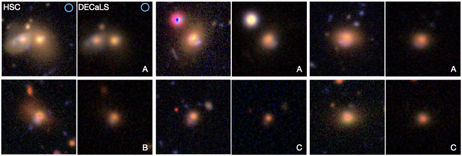
Figure 21: A sample of color images of the HSC lens candidates confirmed with the GaSNets vs. the corresponding DECaLS images. For each strong lens, we show the $gri$ combined images from the HSC database left panel, against the $grz$ color image of the same pointing from DECaLS (right panel). Color combined images are used with the same set-up on the individual band. Part of the lower quality of DECaLS can be due to the $z$-band imaging which was the only redder band available. In each DECaLS panel, we show the visual grading given by us. In the top left pair of figures, we also show the size of the fiber from eBOSS (top-right corner).

References

- Ahn et al. (2012) Ahn, C. P., Alexandroff, R., Allende Prieto, C., et al. 2012, ApJS, 203, 21
- Ahumada et al. (2020) Ahumada, R., Prieto, C. A., Almeida, A., et al. 2020, ApJS, 249, 3
- Auger et al. (2009) Auger, M. W., Treu, T., Bolton, A. S., et al. 2009, ApJ, 705, 1099
- Ball et al. (2007) Ball, N. M., Brunner, R. J., Myers, A. D., et al. 2007, ApJ, 663, 774
- Barnabè et al. (2012) Barnabè, M., Dutton, A. A., Marshall, P. J., et al. 2012, MNRAS, 423, 1073
- Bolton et al. (2008) Bolton, A. S., Burles, S., Koopmans, L. V. E., et al. 2008, ApJ, 682, 964
- Bolton et al. (2004) Bolton, A. S., Burles, S., Schlegel, D. J., Eisenstein, D. J., & Brinkmann, J. 2004, AJ, 127, 1860
- Bolton et al. (2012) Bolton, A. S., Brownstein, J. R., Kochanek, C. S., et al. 2012, ApJ, 757, 82
- Bonjean et al. (2019) Bonjean, V., Aghanim, N., Salomé, P., et al. 2019, A&A, 622, A137
- Brownstein et al. (2012) Brownstein, J. R., Bolton, A. S., Schlegel, D. J., et al. 2012, ApJ, 744, 41
- Cao et al. (2020) Cao, X., Li, R., Shu, Y., et al. 2020, MNRAS, 499, 3610
- Chan et al. (2016) Chan, J. H. H., Suyu, S. H., More, A., et al. 2016, ApJ, 832, 135
- Chang et al. (2021) Chang, Y.-Y., Hsieh, B.-C., Wang, W.-H., et al. 2021, ApJ, 920, 68
- Cornachione et al. (2018) Cornachione, M. A., Bolton, A. S., Shu, Y., et al. 2018, ApJ, 853, 148
- da Cunha et al. (2017) da Cunha, E., Hopkins, A. M., Colless, M., et al. 2017, PASA, 34, e047
- Dawson et al. (2016) Dawson, K. S., Kneib, J.-P., Percival, W. J., et al. 2016, AJ, 151, 44
- de Jong et al. (2012) de Jong, R. S., Bellido-Tirado, O., Chiappini, C., et al. 2012, in Society of Photo-Optical Instrumentation Engineers (SPIE) Conference Series, Vol. 8446, Ground-based and Airborne Instrumentation for Astronomy IV, ed. I. S. McLean, S. K. Ramsay, & H. Takami, 84460T
- DESI Collaboration et al. (2016) DESI Collaboration, Aghamousa, A., Aguilar, J., et al. 2016, arXiv e-prints, arXiv:1611.00036
- Friedman (1999) Friedman, J. H. 1999, Annals of Statistics, 29, 1189
- Gavazzi et al. (2014) Gavazzi, R., Marshall, P. J., Treu, T., & Sonnenfeld, A. 2014, ApJ, 785, 144
- Ghosh et al. (2021) Ghosh, A., Williams, L. L. R., Liesenborgs, J., et al. 2021, MNRAS, 506, 6144
- Gilman et al. (2018) Gilman, D., Birrer, S., Treu, T., Keeton, C. R., & Nierenberg, A. 2018, MNRAS, 481, 819
- Han et al. (2021) Han, B., Qiao, L. N., Chen, J. L., et al. 2021, Research in Astronomy and Astrophysics, 21, 017 (13pp)
- He et al. (2021) He, Z.-H., Xu, Y., Hao, C.-J., Wu, Z.-Y., & Li, J.-J. 2021, Research in Astronomy and Astrophysics, 21, 093
- Holwerda et al. (2022) Holwerda, B. W., Knabel, S., Thorne, J. E., et al. 2022, MNRAS, 510, 2305
- Jacobs et al. (2019) Jacobs, C., Collett, T., Glazebrook, K., et al. 2019, VizieR Online Data Catalog, J/ApJS/243/17
- Jadhav et al. (2021) Jadhav, V. V., Pennock, C. M., Subramaniam, A., Sagar, R., & Nayak, P. K. 2021, MNRAS, 503, 236
- Khramtsov et al. (2019) Khramtsov, V., Sergeyev, A., Spiniello, C., et al. 2019, A&A, 632, A56
- Koopmans et al. (2006) Koopmans, L. V. E., Treu, T., Bolton, A. S., Burles, S., & Moustakas, L. A. 2006, ApJ, 649, 599
- Koopmans et al. (2009) Koopmans, L. V. E., Bolton, A., Treu, T., et al. 2009, ApJ, 703, L51
- Lemon et al. (2020) Lemon, C., Auger, M. W., McMahon, R., et al. 2020, MNRAS, 494, 3491
- Li et al. (2021a) Li, R., Napolitano, N. R., Roy, N., et al. 2021a, arXiv e-prints, arXiv:2111.05434
- Li et al. (2019) Li, R., Shu, Y., Su, J., et al. 2019, MNRAS, 482, 313
- Li et al. (2018) Li, R., Shu, Y., & Wang, J. 2018, MNRAS, 480, 431
- Li et al. (2020) Li, R., Napolitano, N. R., Tortora, C., et al. 2020, ApJ, 899, 30
- Li et al. (2021b) Li, R., Napolitano, N. R., Spiniello, C., et al. 2021b, ApJ, 923, 16
- MacBride et al. (2021) MacBride, C. D., Jess, D. B., Grant, S. D. T., et al. 2021, Philosophical Transactions of the Royal Society of London Series A, 379, 20200171
- Mandelbaum et al. (2019) Mandelbaum, R., Blazek, J., Chisari, N. E., et al. 2019, BAAS, 51, 363
- Metcalf et al. (2019) Metcalf, R. B., Meneghetti, M., Avestruz, C., et al. 2019, A&A, 625, A119
- Napolitano et al. (2020) Napolitano, N. R., Li, R., Spiniello, C., et al. 2020, ApJ, 904, L31
- Nord et al. (2020) Nord, B., Buckley-Geer, E., Lin, H., et al. 2020, MNRAS, 494, 1308
- Ntampaka et al. (2016) Ntampaka, M., Trac, H., Sutherland, D. J., et al. 2016, ApJ, 831, 135
- Petrillo et al. (2019) Petrillo, C. E., Tortora, C., Chatterjee, S., et al. 2019, MNRAS, 482, 807
- Rusu et al. (2020) Rusu, C. E., Wong, K. C., Bonvin, V., et al. 2020, MNRAS, 498, 1440
- Schlegel et al. (2009) Schlegel, D., White, M., & Eisenstein, D. 2009, in astro2010: The Astronomy and Astrophysics Decadal Survey, Vol. 2010, 314
- Schuldt et al. (2019) Schuldt, S., Chirivì, G., Suyu, S. H., et al. 2019, A&A, 631, A40
- Shu et al. (2015) Shu, Y., Bolton, A. S., Brownstein, J. R., et al. 2015, ApJ, 803, 71
- Shu et al. (2016a) Shu, Y., Bolton, A. S., Kochanek, C. S., et al. 2016a, ApJ, 824, 86
- Shu et al. (2016b) Shu, Y., Bolton, A. S., Mao, S., et al. 2016b, ApJ, 833, 264
- Shu et al. (2017) Shu, Y., Brownstein, J. R., Bolton, A. S., et al. 2017, ApJ, 851, 48
- Sluse et al. (2019) Sluse, D., Rusu, C. E., Fassnacht, C. D., et al. 2019, MNRAS, 490, 613
- Sonnenfeld et al. (2019) Sonnenfeld, A., Jaelani, A. T., Chan, J., et al. 2019, A&A, 630, A71
- Sonnenfeld et al. (2014) Sonnenfeld, A., Nipoti, C., & Treu, T. 2014, ApJ, 786, 89
- Sonnenfeld et al. (2013) Sonnenfeld, A., Treu, T., Gavazzi, R., et al. 2013, ApJ, 777, 98
- Sonnenfeld et al. (2015) Sonnenfeld, A., Treu, T., Marshall, P. J., et al. 2015, in American Astronomical Society Meeting Abstracts, Vol. 225, American Astronomical Society Meeting Abstracts #225, 309.02
- Sonnenfeld et al. (2018) Sonnenfeld, A., Chan, J. H. H., Shu, Y., et al. 2018, PASJ, 70, S29
- Spiniello et al. (2019a) Spiniello, C., Agnello, A., Sergeyev, A. V., et al. 2019a, MNRAS, 483, 3888
- Spiniello et al. (2011) Spiniello, C., Koopmans, L. V. E., Trager, S. C., Czoske, O., & Treu, T. 2011, MNRAS, 417, 3000
- Spiniello et al. (2019b) Spiniello, C., Sergeyev, A. V., Marchetti, L., et al. 2019b, MNRAS, 485, 5086
- Suyu et al. (2013) Suyu, S. H., Auger, M. W., Hilbert, S., et al. 2013, ApJ, 766, 70
- Suyu et al. (2017) Suyu, S. H., Bonvin, V., Courbin, F., et al. 2017, MNRAS, 468, 2590
- Szalay et al. (1999) Szalay, A. S., Kunszt, P., Thakar, A., & Gray, J. 1999, arXiv e-prints, cs/9907009
- Talbot et al. (2021) Talbot, M. S., Brownstein, J. R., Dawson, K. S., Kneib, J.-P., & Bautista, J. 2021, MNRAS, 502, 4617
- Teimoorinia & Keown (2018) Teimoorinia, H., & Keown, J. 2018, MNRAS, 478, 3177
- Tortora et al. (2010) Tortora, C., Napolitano, N. R., Romanowsky, A. J., & Jetzer, P. 2010, ApJ, 721, L1
- Veilleux et al. (2020) Veilleux, S., Maiolino, R., Bolatto, A. D., & Aalto, S. 2020, A&A Rev., 28, 2
- Witstok et al. (2021) Witstok, J., Smit, R., Maiolino, R., et al. 2021, MNRAS, 508, 1686
- Wong et al. (2020) Wong, K. C., Suyu, S. H., Chen, G. C. F., et al. 2020, MNRAS, 498, 1420
- Yang et al. (2021) Yang, D.-M., Xie, Z.-L., & Wang, J.-X. 2021, Research in Astronomy and Astrophysics, 21, 099
- York et al. (2000) York, D. G., Adelman, J., Anderson, John E., J., et al. 2000, AJ, 120, 1579
- Zhu et al. (2021) Zhu, K., Kang, S.-J., & Zheng, Y.-G. 2021, Res. Astron. Astrophys., 21, 015