High-Dimensional Time-Varying Coefficient Estimation

Abstract

In this paper, we develop a novel high-dimensional time-varying coefficient estimation method, based on high-dimensional Itô diffusion processes. To account for high-dimensional time-varying coefficients, we first estimate local (or instantaneous) coefficients using a time-localized Dantzig selection scheme under a sparsity condition, which results in biased local coefficient estimators due to the regularization. To handle the bias, we propose a debiasing scheme, which provides well-performing unbiased local coefficient estimators. With the unbiased local coefficient estimators, we estimate the integrated coefficient, and to further account for the sparsity of the coefficient process, we apply thresholding schemes. We call this Thresholding dEbiased Dantzig (TED). We establish asymptotic properties of the proposed TED estimator. In the empirical analysis, we apply the TED procedure to analyzing high-dimensional factor models using high-frequency data.

Keywords: Dantzig selection, debiased, diffusion process, factor model, high-frequency data, sparsity

1 Introduction

To explain various data types, numerous regression-based models have been developed. Especially, advances in technology provide us big data, which causes the curse of dimensionality problem. To tackle this problem in the high-dimensional regression, we usually assume the sparsity of variables, that is, the number of significant coefficients is small. To accommodate the sparsity condition, we often employ the LASSO procedure (Tibshirani,, 1996), SCAD (Fan and Li,, 2001), and Dantzig selector (Candes and Tao,, 2007). The works of Belloni et al., (2014); Feng et al., (2020); Yuan and Lin, (2006); Zou, (2006) are useful for further reading. There are numerous related papers that can be found in the above literature. These estimation methods result in sparse coefficients, and under the sparsity condition, they are consistent estimators (Negahban et al.,, 2012). Under the diffusion process, Ciolek et al., (2022) studied the properties of the LASSO estimator of the drift component and Gaïffas and Matulewicz, (2019) proposed the estimation procedure for the drift parameter in the high-dimensional Ornstein–Uhlenbeck (OU) process.

On the other hand, in high-frequency finance, we often observe that coefficients in the regression model are time-varying. For example, Andersen et al., (2021) investigated the intra-day variation of the local coefficients, which are called the market betas, between the individual assets and market index. To account for the time-varying feature, Mykland and Zhang, (2009) computed the market beta as the aggregation of the market betas estimated over local blocks. To evaluate the coefficients of multi factor models, Aït-Sahalia et al., (2020) proposed an integrated coefficient approach using the local coefficient. See also Chen, (2018); Oh et al., (2022). We call this high-frequency regression. In the field of finance, there are hundreds of potential factor candidates that explain the cross section of expected stock returns (Cochrane,, 2011; Harvey et al.,, 2016; Hou et al.,, 2020; McLean and Pontiff,, 2016). Thus, we also encounter the curse of dimensionality in high-frequency regressions, so the estimation methods developed for the finite dimension fail to estimate the coefficients consistently. Thus, to fully benefit from the utilization of high-frequency financial data in the high-dimensional regression, we need to develop methodologies that can handle both the curse of dimensionality as well as the time-varying coefficients.

In this paper, we introduce a novel high-dimensional high-frequency regression estimation procedure which can accommodate the sparse and time-varying coefficient processes. To model the high-frequency data, we employ diffusion processes whose stochastic difference equations have a time series regression structure. We also assume that the coefficient beta process $\boldsymbol{\beta}_{t}$ follows a diffusion process. In this paper, the parameter of interest is the integrated beta, $\int_{0}^{1}\boldsymbol{\beta}_{t}dt$. To handle the curse of dimensionality, we assume that the beta processes are sparse, and to account for the sparsity of the time-varying beta process, we employ the Dantzig selector procedure (Candes and Tao,, 2007). Specifically, due to the time-varying phenomena, we cannot estimate the integrated beta directly, and so we first estimate the instantaneous (or local) betas using the time-localized Dantzig selector procedure, based on the definition of $\boldsymbol{\beta}_{t}$. Then, to mitigate the bias coming from the regularization of the Dantzig selector, we propose a debiasing scheme and estimate the integrated beta with the debiased Dantzig instantaneous beta. With the debiasing scheme, we can obtain more accurate estimators in terms of the element-wise convergence rate; however, the estimated integrated beta is not sparse. Thus, to accommodate the sparsity, we further regularize the estimated integrated beta. We call this Thresholding dEbiased Dantzig (TED). We also establish its asymptotic properties.

The rest of paper is organized as follows. Section 2 introduces the model set-up. Section 3 proposes the TED estimation procedure and establishes its asymptotic properties. In Section 4, we conduct a simulation study to check the finite sample performance of the TED estimation procedure, and in Section 5, we apply the TED to the high-frequency financial data. The conclusion is presented in Section 6, and we collect all of the proofs in the supplementary materials.

2 The model set-up

We consider the following non-parametric time series regression diffusion model:

$$dY_{t}=\boldsymbol{\beta}_{t}^{\top}d\mathbf{X}_{t}+dZ_{t},$$ (2.1)

where $Y_{t}$ is a dependent process, $\mathbf{X}_{t}$ is a $p$-dimensional multivariate covariate process, $\boldsymbol{\beta}_{t}$ is a coefficient process, and $Z_{t}$ is a residual process. The $p$-dimensional covariate process $\mathbf{X}_{t}$ and residual process $Z_{t}$ satisfy the following diffusion processes:

$$d\mathbf{X}_{t}=\boldsymbol{\mu}_{t}dt+\boldsymbol{\sigma}_{t}d\mathbf{B}_{t}\quad\text{and}\quad dZ_{t}=\nu_{t}dW_{t},$$

where $\boldsymbol{\mu}_{t}$ is a drift process, $\boldsymbol{\sigma}_{t}$ and $\nu_{t}$ are instantaneous volatility processes, $\mathbf{B}_{t}$ and $W_{t}$ are $p$-dimensional and one-dimensional standard Brownian motions, respectively, and $\mathbf{B}_{t}$ and $W_{t}$ are independent. The processes $\boldsymbol{\mu}_{t}$, $\boldsymbol{\beta}_{t}$, $\boldsymbol{\sigma}_{t}$, and $\nu_{t}$ are predictable. To account for the time-varying coefficient, we further assume that the coefficient $\boldsymbol{\beta}_{t}$ satisfies the following diffusion process:

$$d\boldsymbol{\beta}_{t}=\boldsymbol{\mu}_{\beta,t}dt+\boldsymbol{\nu}_{\beta,t}d\mathbf{W}_{t}^{\beta},$$ (2.2)

where $\boldsymbol{\mu}_{\beta,t}$ and $\boldsymbol{\nu}_{\beta,t}$ are predictable, and $\mathbf{W}_{t}^{\beta}$ is $p$-dimensional standard Brownian motion. The parameter of interest is the integrated beta:

$$I\beta=(I\beta_{i})_{i=1,\ldots,p}=\int_{0}^{1}\boldsymbol{\beta}_{t}dt.$$

In finance, hundreds of potential factor candidates have been proposed in order to explain the cross section of expected stock returns (Cochrane,, 2011; Harvey et al.,, 2016; Hou et al.,, 2020; McLean and Pontiff,, 2016). That is, the dimensionality, $p$, of the covariate process is large. Thus, we often run into the curse of dimensionality problem when handling financial data. However, all of them may not be significant; thus, to account for this, we assume that the coefficient process $\boldsymbol{\beta}_{t}=(\beta_{1t},\ldots,\beta_{pt})^{\top}$ satisfies the following sparsity condition:

$$\sup_{0\leq t\leq 1}\sum_{i=1}^{p}|\beta_{it}|^{\delta}\leq s_{p}\quad\text{and}\quad\sum_{i=1}^{p}|I\beta_{i}|^{\delta}\leq s_{p}\,\text{ a.s.},$$ (2.3)

where $0^{0}$ is defined as 0, $\delta\in[0,1)$, and $s_{p}$ is diverging slowly with respect to $p$, for example, $\log p$. We investigate asymptotic properties under this general sparsity case. However, in practice, it is harmless to assume $\delta=0$. That is, we can assume that several factors are significant, while others do not affect on the expected returns. We note that with the randomness of the beta process, in general, the sparsity condition (2.3) is satisfied with high probability. However, for simplicity, we assume that the sparsity condition is satisfied almost surely. The sparsity condition is widely employed in the high-frequency finance literature (Ciolek et al.,, 2022; Gaïffas and Matulewicz,, 2019; Kim et al.,, 2016, 2018; Tao et al.,, 2013; Wang and Zou,, 2010).

3 High-dimensional high-frequency regression

3.1 Estimation procedure

In this section, we propose an estimation procedure for large integrated betas. We first fix some notations. For any given $p_{1}$ by $p_{2}$ matrix $\mathbf{U}=\left(U_{ij}\right)$, let

$$\|\mathbf{U}\|_{\max}=\max_{i,j}|U_{ij}|,\quad\|\mathbf{U}\|_{1}=\max\limits_{1\leq j\leq p_{2}}\sum\limits_{i=1}^{p_{1}}|U_{ij}|,\quad\text{ and }\quad\|\mathbf{U}\|_{\infty}=\max\limits_{1\leq i\leq p_{1}}\sum\limits_{j=1}^{p_{2}}|U_{ij}|.$$

We denote the Frobenius norm of $\mathbf{U}$ by $\|\mathbf{U}\|_{F}=\sqrt{\mathrm{tr}(\mathbf{U}^{\top}\mathbf{U})}$. The matrix spectral norm $\|\mathbf{U}\|_{2}$ is the square root of the largest eigenvalue of $\mathbf{U}\mathbf{U}^{\top}$. $C$’s denote generic constants whose values are free of $n$ and $p$ and may change from appearance to appearance.

From the model (2.1), the instantaneous beta $\boldsymbol{\beta}_{t}$ satisfies the following equation:

$$\frac{d}{dt}[Y,\mathbf{X}]_{t}=\boldsymbol{\beta}_{t}^{\top}\frac{d}{dt}[\mathbf{X},\mathbf{X}]_{t}\,\text{ a.s.},$$

where $[\cdot,\cdot]$ denotes the quadratic variation. The beta process $\boldsymbol{\beta}_{t}$ is a function of instantaneous volatilities of $\mathbf{X}$ and $Y$ as follows:

$$\boldsymbol{\beta}_{t}=\boldsymbol{\Sigma}_{t}^{-1}\boldsymbol{\Sigma}_{XY,t}\,\text{ a.s.},$$ (3.1)

where $\boldsymbol{\Sigma}_{t}=\boldsymbol{\sigma}_{t}\boldsymbol{\sigma}_{t}^{\top}$ and $\boldsymbol{\Sigma}_{XY,t}=\frac{d}{dt}[\mathbf{X},Y]_{t}$. Thus, the instantaneous beta can be estimated by the instantaneous volatility estimators. For the finite dimensional case, the instantaneous volatility-based estimation procedure works well (Aït-Sahalia et al.,, 2020). However, this approach cannot explain the sparse structure (2.3). Furthermore, when the dimensionality of the covariate $\mathbf{X}$ is larger than the sample size, this approach fails to consistently estimate the instantaneous beta. Therefore, the procedure developed for the finite dimension is neither effective nor efficient. To accommodate the sparse structure of the beta process in (2.3), we employ the Dantzig selection method (Candes and Tao,, 2007) as follows. Let $\Delta_{i}^{n}A=A_{i\Delta_{n}}-A_{(i-1)\Delta_{n}}$ for $1\leq i\leq 1/\Delta_{n}$, where $\Delta_{n}=1/n$ is the distance between adjacent observation time points. Define

$$\mathcal{Y}_{i}=\begin{pmatrix}\Delta_{i+1}^{n}Y\\ \Delta_{i+2}^{n}Y\\ \vdots\\ \Delta_{i+k_{n}}^{n}Y\end{pmatrix},\quad\mathcal{X}_{i}=\begin{pmatrix}\Delta_{i+1}^{n}\mathbf{X}^{\top}\\ \Delta_{i+2}^{n}\mathbf{X}^{\top}\\ \vdots\\ \Delta_{i+k_{n}}^{n}\mathbf{X}^{\top}\end{pmatrix},\quad\text{and}\quad\mathcal{Z}_{i}=\begin{pmatrix}\Delta_{i+1}^{n}Z\\ \Delta_{i+2}^{n}Z\\ \vdots\\ \Delta_{i+k_{n}}^{n}Z\end{pmatrix},$$

where $k_{n}$ is the number of observations in each window to calculate the local regression. Then, we estimate the sparse instantaneous beta as follows:

$$\widehat{\boldsymbol{\beta}}_{i\Delta_{n}}=\arg\min\|\boldsymbol{\beta}\|_{1}\quad\text{ s.t. }\left\|\frac{1}{k_{n}\Delta_{n}}\mathcal{X}_{i}^{\top}\mathcal{X}_{i}\boldsymbol{\beta}-\frac{1}{k_{n}\Delta_{n}}\mathcal{X}_{i}^{\top}\mathcal{Y}_{i}\right\|_{\max}\leq\lambda_{n},$$ (3.2)

where $\lambda_{n}$ is a tuning parameter which converges to zero. We specify $\lambda_{n}$ in Theorem 1. With the appropriate $\lambda_{n}$, we can show that the proposed Dantzig instantaneous beta estimator $\widehat{\boldsymbol{\beta}}_{i\Delta_{n}}$ is a consistent estimator (see Theorem 1). To estimate the integrated beta $I\beta$ with this consistent estimator, we usually consider the sum of the instantaneous volatility estimators $\widehat{\boldsymbol{\beta}}_{i\Delta_{n}}$’s. However, the Dantzig estimator is biased, so their summation cannot enjoy the law of large number properties. For example, the error of the sum of the Dantzig instantaneous beta estimators is dominated by the bias terms, and so it has the same convergence rate as that of $\widehat{\boldsymbol{\beta}}_{i\Delta_{n}}$. To reduce the effect of the bias, we use a debiasing scheme as follows. We first estimate the inverse matrix of the instantaneous volatility matrix $\boldsymbol{\Sigma}_{i\Delta_{n}}$ using the constrained $\ell_{1}$-minimization for inverse matrix estimation (CLIME) (Cai et al.,, 2011). Let $\widehat{\boldsymbol{\Omega}}_{i\Delta_{n}}$ be the solution of the following optimization problem:

$$\min\|\boldsymbol{\Omega}\|_{1}\quad\text{s.t.}\quad\|\frac{1}{k_{n}\Delta_{n}}\mathcal{X}_{i}^{\top}\mathcal{X}_{i}\boldsymbol{\Omega}-\mathbf{I}\|_{\max}\leq\tau_{n},$$ (3.3)

where $\tau_{n}$ is the tuning parameter specified in Theorem 2. With the CLIME estimator, we adjust the Dantzig instantaneous beta estimator as follows:

$$\widetilde{\boldsymbol{\beta}}_{i\Delta_{n}}=\widehat{\boldsymbol{\beta}}_{i\Delta_{n}}+\frac{1}{k_{n}\Delta_{n}}\widehat{\boldsymbol{\Omega}}_{i\Delta_{n}}^{\top}\mathcal{X}_{i}^{\top}(\mathcal{Y}_{i}-\mathcal{X}_{i}\widehat{\boldsymbol{\beta}}_{i\Delta_{n}}).$$ (3.4)

Then, the debiased Dantzig instantaneous beta estimator satisfies

$$\widetilde{\boldsymbol{\beta}}_{i\Delta_{n}}-\boldsymbol{\beta}_{0,i\Delta_{n}}=\frac{1}{k_{n}\Delta_{n}}\boldsymbol{\Omega}_{0,i\Delta_{n}}\left(\mathcal{X}_{i}^{\top}\mathcal{Z}_{i}+\mathcal{A}_{i}\right)+R_{i}\text{ a.s.},$$

where the subscript $0$ represents the true parameters, $\mathcal{A}_{i}$ is a martingale difference defined in (A.24), and $R_{i}$ is a negligible remaining error term (see Theorem 3). We note that the debiasing scheme is usually employed to derive asymptotic normality and to conduct the confidence interval construction or hypothesis test (Javanmard and Montanari,, 2018; Van de Geer et al.,, 2014; Zhang and Zhang,, 2014). However, we adopt the debiasing scheme to improve the integrated beta estimation. Specifically, the debiasing scheme helps enjoy the law of large number property when averaging the instantaneous beta estimators. The integrated beta estimator is defined by

$$\widehat{I\beta}=\sum_{i=0}^{[1/(k_{n}\Delta_{n})]-1}\widetilde{\boldsymbol{\beta}}_{ik_{n}\Delta_{n}}k_{n}\Delta_{n}.$$

As discussed above, the debiasing scheme helps improve the element-wise convergence rate of the debiased Dantzig integrated beta estimator. However, the debiased Dantzig integrated beta estimator does not satisfy the sparsity condition (2.3) due to the bias adjustment. To accommodate the sparsity of the integrated beta, we apply the thresholding scheme as follows:

$$\widetilde{I\beta}_{i}=s(\widehat{I\beta}_{i})\boldsymbol{1}\left(|\widehat{I\beta}_{i}|\geq h_{n}\right)\quad\text{and}\quad\widetilde{I\beta}=\left(\widetilde{I\beta}_{i}\right)_{i=1,\ldots,p},$$

where $\boldsymbol{1}(\cdot)$ is an indicator function, the thresholding function $s(\cdot)$ satisfies that $|s(x)-x|\leq h_{n}$, and $h_{n}$ is a thresholding level specified in Theorem 4. Examples of the thresholding function $s(x)$ include the hard thresholding function $s(x)=x$ and the soft thresholding function $s(x)=x-\mbox{sign}(x)h_{n}$. For the empirical study, we employed the hard thresholding function. We call this the Thresholded dEbiased Dantzig (TED) estimator. We summarize the TED estimation procedure in Algorithm 1.

Algorithm 1 TED estimation procedure

Step 1 Estimate the instantaneous beta:

$$\widehat{\boldsymbol{\beta}}_{i\Delta_{n}}=\arg\min\|\boldsymbol{\beta}\|_{1}\quad\text{ s.t. }\left\|\frac{1}{k_{n}\Delta_{n}}\mathcal{X}_{i}^{\top}\mathcal{X}_{i}\boldsymbol{\beta}-\frac{1}{k_{n}\Delta_{n}}\mathcal{X}_{i}^{\top}\mathcal{Y}_{i}\right\|_{\max}\leq\lambda_{n},$$

where $\lambda_{n}=C_{\lambda}s_{p}\sqrt{\log p}\left(\sqrt{k_{n}\Delta_{n}}+k_{n}^{-1/2}\right)$ and $k_{n}=c_{k}n^{1/2}$ for some large constants $C_{\lambda}$ and $c_{k}$.

Step 2 Estimate the inverse instantaneous volatility matrix:

$$\widehat{\boldsymbol{\Omega}}_{i\Delta_{n}}=\arg\min\|\boldsymbol{\Omega}\|_{1}\quad\text{s.t.}\quad\|\frac{1}{k_{n}\Delta_{n}}\mathcal{X}_{i}^{\top}\mathcal{X}_{i}\boldsymbol{\Omega}-\mathbf{I}\|_{\max}\leq\tau_{n},$$

where $\tau_{n}=C_{\tau}\sqrt{\log p}\left(\sqrt{k_{n}\Delta_{n}}+k_{n}^{-1/2}\right)$ for some large constant $C_{\tau}$.

Step 3 Debias the Dantzig instantaneous beta estimator:

$$\widetilde{\boldsymbol{\beta}}_{i\Delta_{n}}=\widehat{\boldsymbol{\beta}}_{i\Delta_{n}}+\frac{1}{k_{n}\Delta_{n}}\widehat{\boldsymbol{\Omega}}_{i\Delta_{n}}^{\top}\mathcal{X}_{i}^{\top}(\mathcal{Y}_{i}-\mathcal{X}_{i}\widehat{\boldsymbol{\beta}}_{i\Delta_{n}}).$$

Step 4 Estimate the integrated beta:

$$\widehat{I\beta}=\sum_{i=0}^{[1/(k_{n}\Delta_{n})]-1}\widetilde{\boldsymbol{\beta}}_{ik_{n}\Delta_{n}}k_{n}\Delta_{n}.$$

Step 5 Threshold the debiased Dantzig integrated beta estimator:

$$\widetilde{I\beta}_{i}=s(\widehat{I\beta}_{i})\boldsymbol{1}\left(|\widehat{I\beta}_{i}|\geq h_{n}\right)\quad\text{and}\quad\widetilde{I\beta}=\left(\widetilde{I\beta}_{i}\right)_{i=1,\ldots,p},$$

where $\boldsymbol{1}(\cdot)$ is an indicator function, the thresholding function $s(\cdot)$ satisfies that $|s(x)-x|\leq h_{n}$, $h_{n}=C_{h}b_{n}$ for some constant $C_{h}$, and $b_{n}$ is defined in Theorem 3.

3.2 Asymptotic results

In this section, we establish the asymptotic properties for the proposed TED estimation procedure. To investigate the asymptotic properties, we need the following technical conditions.

Assumption 1.

• The volatility process $\boldsymbol{\Sigma}_{t}=(\Sigma_{ijt})_{i,j=1,\ldots,p}$ satisfies the following Hölder condition:

  $$|\Sigma_{ijt}-\Sigma_{ijs}|\leq C|t-s|^{1/2}\,\text{ a.s.}$$

• $\boldsymbol{\mu}_{t}$, $\boldsymbol{\mu}_{\beta,t}$, $\boldsymbol{\beta}_{t}$, $\nu_{t}$, $\boldsymbol{\Sigma}_{t}$, and $\boldsymbol{\Sigma}_{\beta,t}=\boldsymbol{\nu}_{\beta,t}\boldsymbol{\nu}_{\beta,t}^{\top}$ are almost surely bounded, and $\|\boldsymbol{\Sigma}_{t}^{-1}\|_{1}\leq C$ a.s.

• The drift process $\boldsymbol{\mu}_{\beta,t}=\left(\mu_{\beta,1t},\ldots,\mu_{\beta,pt}\right)^{\top}$ and the volatility process $\boldsymbol{\Sigma}_{\beta,t}=\left(\Sigma_{\beta,ijt}\right)_{i,j=1,\ldots,p}$ satisfy the following sparsity condition for $\delta\in[0,1)$:

  $$\sup_{0\leq t\leq 1}\sum_{i=1}^{p}|\mu_{\beta,it}|^{\delta}\leq s_{p}\quad\text{and}\quad\sup_{0\leq t\leq 1}\sum_{i=1}^{p}|\Sigma_{\beta,iit}|^{\delta/2}\leq s_{p}\text{ a.s.}$$

• The inverse matrix of the volatility matrix process, $\boldsymbol{\Sigma}_{t}^{-1}=\boldsymbol{\Omega}_{t}=(\omega_{ijt})_{i,j=1,\ldots,p}$, satisfies the following sparsity condition:

  $$\sup_{0\leq t\leq 1}\max_{1\leq i\leq p}\sum_{j=1}^{p}|\omega_{ijt}|^{q}\leq s_{\omega,p}\,\text{ a.s.},$$

  where $q\in[0,1)$ and $s_{\omega,p}$ is diverging slowly with respect to $p$, for example, $\log p$.

• $n^{c_{1}}\leq p\leq c_{2}\exp(n^{c_{3}})$ for some positive constants $c_{1}$, $c_{2}$, and $c_{3}<1/8$, and $s_{p}^{2}\log p\Delta_{n}k_{n}\rightarrow 0$ as $n,p\rightarrow\infty$.

Remark 1.

To investigate estimators of time-varying processes, we need continuity conditions such as Assumption 1(a) and the diffusion process structures for $\mathbf{X}_{t}$, $Y_{t}$ and $\boldsymbol{\beta}_{t}$ in Section 2. Even if Assumption 1(a) is replaced by the condition that $\boldsymbol{\Sigma}_{t}$ has a continuous Itô diffusion process structure with bounded drift and instantaneous volatility processes, we can obtain the same theoretical results with up to $\sqrt{\log p}$ order. For simplicity, we put Assumption 1(a). The boundedness condition Assumption 1(b) provides sub-Gaussian tails which are often required to investigate high-dimensional inferences. On the other hand, when we investigate the asymptotic behaviors of volatility estimators such as their convergence rate, the boundedness condition can be relaxed to the locally boundedness condition (see Aït-Sahalia and Xiu, (2017)). Specifically, Jacod and Protter, (2011) showed in Lemma 4.4.9 that if the asymptotic result, such as stable convergence in law or convergence in probability, is satisfied under the boundedness condition, it is also satisfied under the locally boundedness condition. Thus, the asymptotic results established in this paper also hold for the locally boundedness condition. The sparsity condition for the beta process, Assumption 1(c), is the technical condition for investigating the discretization error of Dantzig instantaneous beta estimator $\widehat{\boldsymbol{\beta}}_{i\Delta_{n}}$. Finally, to investigate asymptotic properties of the CLIME estimator, we need the sparse inverse matrix condition Assumption 1(d) (Cai et al.,, 2011). Furthermore, if the smallest eigenvalue of $\boldsymbol{\Sigma}_{t}$ is strictly bigger than zero, the Frobenius norm of $\boldsymbol{\Omega}_{t}$ is bounded by $C\sqrt{p}$. This implies that the inverse matrix, $\boldsymbol{\Omega}_{t}$, is not dense. Since the strict positiveness of the smallest eigenvalue is the minimum requirement to investigate the regression-based models, Assumption 1(d) is reasonable.

In Theorems 1 and 2 below, we establish asymptotic properties for the sparse instantaneous beta and inverse matrix. Note that we use subscript $0$ for the true parameters.

Theorem 1.

Under Assumption 1(a)–(c), let $k_{n}=c_{k}n^{c}$ for some constants $c_{k}$ and $c\in(1/4,1/2]$. For any given positive constant $a$, choose $\lambda_{n}=C_{\lambda,a}s_{p}\sqrt{\log p}\left(\sqrt{k_{n}\Delta_{n}}+k_{n}^{-1/2}\right)$ for some large constant $C_{\lambda,a}$. Then, we have, for large $n$,

$$\max_{i}\|\widehat{\boldsymbol{\beta}}_{i\Delta_{n}}-\boldsymbol{\beta}_{0,i\Delta_{n}}\|_{\max}\leq C\lambda_{n}\quad\text{and}\quad\max_{i}\|\widehat{\boldsymbol{\beta}}_{i\Delta_{n}}-\boldsymbol{\beta}_{0,i\Delta_{n}}\|_{1}\leq Cs_{p}\lambda_{n}^{1-\delta},$$ (3.5)

with probability greater than $1-p^{-a}$.

Theorem 2.

Under Assumption 1, let $k_{n}=c_{k}n^{c}$ for some constants $c_{k}$ and $c\in(1/4,1/2]$. For any given positive constant $a$, choose $\tau_{n}=C_{\tau,a}\sqrt{\log p}\left(\sqrt{k_{n}\Delta_{n}}+k_{n}^{-1/2}\right)$ for some large constant $C_{\tau,a}$. Then, we have, for large $n$,

$$\max_{i}\|\widehat{\boldsymbol{\Omega}}_{i\Delta_{n}}-\boldsymbol{\Omega}_{0,i\Delta_{n}}\|_{\max}\leq C\tau_{n}\quad\text{and}\quad\max_{i}\|\widehat{\boldsymbol{\Omega}}_{i\Delta_{n}}-\boldsymbol{\Omega}_{0,i\Delta_{n}}\|_{1}\leq Cs_{\omega,p}\tau_{n}^{1-q},$$ (3.6)

with probability greater than $1-p^{-a}$.

Remark 2.

Theorems 1 and 2 show that by choosing $c=1/2$, the estimators for the instantaneous beta and inverse matrix have element-wise convergence rates of $n^{-1/4}$ and $\ell_{1}$ convergence rates $n^{-(1-\delta)/4}$ and $n^{-(1-q)/4}$, respectively, with the $\log$ order term and the sparsity level term. We note that when choosing the sub-interval length $k_{n}=c_{k}n^{1/2}$ to estimate the instantaneous processes, we have the same order convergence rates of the statistical estimation and time-varying instantaneous process approximation errors. That is, the order $n^{-1/4}$ is optimal for estimating each element of the instantaneous process; thus, the convergence rates are optimal up to log order.

The Dantzig instantaneous beta estimator has a near-optimal convergence rate as shown in Theorem 1. However, as discussed in the previous section, it is a biased estimator, which causes some non-negligible estimation errors when estimating the integrated beta. To tackle this problem, we employ debiasing schemes with the consistent CLIME estimator as in (3.4), and in the following theorem, we investigate its asymptotic benefits.

Theorem 3.

Under the assumptions in Theorems 1–2, we choose $k_{n}=c_{k}n^{1/2}$ for some constant $c_{k}$. Then, we have for all $i$,

$$\widetilde{\boldsymbol{\beta}}_{i\Delta_{n}}-\boldsymbol{\beta}_{0,i\Delta_{n}}=\frac{1}{k_{n}\Delta_{n}}\boldsymbol{\Omega}_{0,i\Delta_{n}}\left(\mathcal{X}_{i}^{\top}\mathcal{Z}_{i}+\mathcal{A}_{i}\right)+R_{i},$$ (3.7)

where $\mathcal{A}_{i}$ is defined in (A.24) and

$$\max_{i}\|R_{i}\|_{\max}\leq C\left\{s_{p}^{2-\delta}(\log p/n^{1/2})^{(2-\delta)/2}+s_{p}s_{\omega,p}(\log p/n^{1/2})^{(2-q)/2}+s_{p}(\log p)^{3/2}/n^{1/2}\right\},$$ (3.8)

with probability greater than $1-p^{-a}$ for any given positive constant $a$. Furthermore, we have, with probability greater than $1-p^{-a}$ for any given positive constant $a$,

$$\|\widehat{I\beta}-I\beta_{0}\|_{\max}\leq Cb_{n},$$ (3.9)

where $b_{n}=s_{p}^{2-\delta}(\log p/n^{1/2})^{(2-\delta)/2}+s_{p}s_{\omega,p}(\log p/n^{1/2})^{(2-q)/2}+s_{p}(\log p)^{3/2}/n^{1/2}$.

Remark 3.

The debiased Dantzig instantaneous beta is decomposed by the martingale difference term $\mathcal{X}_{i}^{\top}\mathcal{Z}_{i}+\mathcal{A}_{i}$ and the non-martingale remaining term $R_{i}$. The martingale difference term can enjoy the law of large number property, so the integrated beta estimator has a faster convergence rate than the Dantzig instantaneous beta estimator. The remaining non-martingale terms have the same order as those of the martingale terms for the integrated beta estimator. Unlike the biased Dantzig estimator, the non-martingale remaining terms do not impact on the integrated beta estimator.

Remark 4.

Theorem 3 shows the element-wise convergence rate for the debiased Dantzig integrated beta. When we have the exact sparse beta and inverse matrix processes, that is, $\delta=q=0$, the debiased Dantzig integrated beta estimator has the convergence rate $s_{p}(s_{p}+s_{\omega,p})(\log p)^{3/2}/n^{1/2}$. The $n^{1/2}$ term is related with the sample size, which is known as the optimal rate. The $(\log p)^{3/2}$ term comes from handling the high-dimensional error bound. Usually, in high-dimensional literature, we have $\sqrt{\log p}$, but the debiased Dantzig integrated beta estimator has $(\log p)^{3/2}$ due to the handling of the high-dimensional error bounds for estimating two betas, such as the instantaneous beta and the integrated beta, and bounding the random processes. Finally, the $s_{p}$ and $s_{\omega,p}$ terms represent the sparsity levels for the beta and inverse volatility matrix. High-dimensional literature commonly assumes the sparsity level to be negligible; hence, we have the convergence rate $n^{-1/2}$ with up to $\log p$ order.

Theorem 3 indicates that, using the debiasing scheme, we obtain well-performing input integrated beta estimator $\widehat{\boldsymbol{\beta}}$. As described in Section 3.1, with the input integrated beta estimator $\widehat{\boldsymbol{\beta}}$, we apply the thresholding scheme to account for the sparsity and obtain the TED estimator. In the following theorem, we establish the $\ell_{1}$ convergence rate of the TED estimator.

Theorem 4.

Under the assumptions in Theorems 1–2, let $k_{n}=c_{k}n^{1/2}$ for some constant $c_{k}$. For any given positive constant $a$, choose $h_{n}=C_{h,a}b_{n}$ for some constant $C_{h,a}$, where $b_{n}$ is defined in Theorem 3. Then, we have, with probability greater than $1-p^{-a}$,

$$\|\widetilde{I\beta}-I\beta_{0}\|_{1}\leq Cs_{p}b_{n}^{1-\delta}.$$ (3.10)

Theorem 4 shows that the TED estimator is a consistent estimator in terms of the $\ell_{1}$ norm under the sparsity condition (2.3). When estimating the integrated beta without the debiasing step, we can obtain the convergence rate $s_{p}(s_{p}\sqrt{\log p}n^{-1/4})^{1-\delta}$. The benefit of applying the debiasing scheme is the difference between $b_{n}$ and $s_{p}\sqrt{\log p}n^{-1/4}$. Under the sparsity condition, $b_{n}$ is $n^{-\{2-(\delta\vee q)\}/4}$ with $\log p$ order for $\delta,q\in[0,1)$, which is faster than the convergence rate of the Dantzig integrated beta estimator. Therefore, the TED estimator has the faster convergence rate.

3.3 Extension to jump diffusion processes

In financial practice, we often observe jumps. To reflect this, we can extend the continuous diffusion process (2.1) to the jump diffusion process as follows:

$$dY_{t}=dY^{c}_{t}+dY^{J}_{t},$$ (3.11)

$$dY^{c}_{t}=\boldsymbol{\beta}_{t}^{\top}d\mathbf{X}^{c}_{t}+dZ_{t},\quad\text{and}\quad dY^{J}_{t}=J^{y}_{t}d\Lambda^{y}_{t},$$ (3.12)

where $Y_{t}^{c}$ and $\mathbf{X}_{t}^{c}$ are the continuous part of $Y_{t}$ and $\mathbf{X}_{t}$, respectively, $J_{t}^{y}$ is the jump size, and $\Lambda_{t}^{y}$ is the Poisson process with the bounded intensity. The covariate process $\mathbf{X}_{t}$ is

$$d\mathbf{X}_{t}=d\mathbf{X}_{t}^{c}+d\mathbf{X}_{t}^{J},\quad d\mathbf{X}_{t}^{c}=\boldsymbol{\mu}_{t}dt+\boldsymbol{\sigma}_{t}d\mathbf{B}_{t},\quad\text{and}\quad d\mathbf{X}_{t}^{J}=\mathbf{J}_{t}d\boldsymbol{\Lambda}_{t},$$ (3.13)

where $\mathbf{J}_{t}=\left(J_{1t},\ldots,J_{pt}\right)^{\top}$ is a jump size process and $\boldsymbol{\Lambda}_{t}=\left(\Lambda_{1t},\ldots,\Lambda_{pt}\right)^{\top}$ is a $p$-dimensional Poisson process with bounded intensities. We assume that the Poisson processes $\Lambda_{t}^{y}$ and $\boldsymbol{\Lambda}_{t}$ are independent of $\boldsymbol{\sigma}_{t}$ and $\boldsymbol{\beta}_{t}$. Under this jump diffusion model, we can still use the proposed estimation procedure, but we cannot observe the continuous diffusion process. To tackle this problem, we first detect the jumps from the observed stock log-return data. For example, we use the truncation method as follows. Define

$$\widehat{\mathcal{Y}}_{i}^{c}=\begin{pmatrix}\Delta_{i+1}^{n}\widehat{Y}^{c}\\ \Delta_{i+2}^{n}\widehat{Y}^{c}\\ \vdots\\ \Delta_{i+k_{n}}^{n}\widehat{Y}^{c}\end{pmatrix}\quad\text{ and }\quad\widehat{\mathcal{X}}_{i}^{c}=\begin{pmatrix}\Delta_{i+1}^{n}\widehat{\mathbf{X}}^{c\top}\\ \Delta_{i+2}^{n}\widehat{\mathbf{X}}^{c\top}\\ \vdots\\ \Delta_{i+k_{n}}^{n}\widehat{\mathbf{X}}^{c\top}\end{pmatrix},$$ (3.14)

where $\boldsymbol{1}_{\{\cdot\}}$ is an indicator function, $k_{n}$ is the number of observations in each window used to calculate the local regression,

$$\Delta_{i}^{n}\widehat{Y}^{c}=\Delta_{i}^{n}Y\,\boldsymbol{1}_{\{|\Delta_{i}^{n}Y|\leq u_{n}\}},\quad\Delta_{i}^{n}\widehat{\mathbf{X}}^{c}=\left(\Delta_{i}^{n}X_{j}\,\boldsymbol{1}_{\{|\Delta_{i}^{n}X_{j}|\leq v_{j,n}\}}\right)_{j=1,\ldots,p},$$

and $u_{n}$ and $v_{j,n}$, $j=1,\ldots,p$, are the truncation levels. We employ $u_{n}=C_{u}s_{p}\sqrt{\log p}n^{-\varrho}$ and $v_{j,n}=C_{j,v}\sqrt{\log p}n^{-\varrho}$ for $\varrho\in[15/32,1/2)$ and some constants $C_{u}$ and $C_{j,v}$, $j=1,\ldots,p$. In the numerical study, we adopt the usual choice in the literature (Aït-Sahalia et al.,, 2020; Aït-Sahalia and Xiu,, 2019). That is, we use

$$u_{n}=3n^{-0.47}\sqrt{BV^{Y}}\quad\text{and}\quad v_{j,n}=3n^{-0.47}\sqrt{BV_{j}},$$ (3.15)

where the bipower variations $BV^{Y}=\dfrac{\pi}{2}\sum_{i=2}^{n}|\Delta_{i-1}^{n}Y|\cdot|\Delta_{i}^{n}Y|$ and $BV_{j}=\dfrac{\pi}{2}\sum_{i=2}^{n}|\Delta_{i-1}^{n}X_{j}|\cdot|\Delta_{i}^{n}X_{j}|$. Then, to estimate the integrated beta $I\beta$, we employ the estimation method in Section 3.1 using $\widehat{\mathcal{Y}}_{i}^{c}$ and $\widehat{\mathcal{X}}_{i}^{c}$ instead of $\mathcal{Y}_{i}$ and $\mathcal{X}_{i}$. We denote the jump-adjusted TED estimator by $\widetilde{I\beta}^{c}$. In the following theorem, we investigate the asymptotic property of the jump-adjusted TED estimator.

Theorem 5.

Under the models (3.11)–(3.13), let assumptions in Theorem 4 hold. Then, we have, with probability greater than $1-p^{-a}$ for any given positive constant $a$,

$$\|\widetilde{I\beta}^{c}-I\beta_{0}\|_{1}\leq Cs_{p}b_{n}^{1-\delta}.$$ (3.16)

Theorem 5 shows that the jump-adjusted TED estimator has the same convergence rate obtained in Theorem 4. Therefore, we conclude that the jumps can be detected well and that their effects can be mitigated.

3.4 Discussion on the tuning parameter selection

To implement the TED estimation procedure, we need to choose the tuning parameters. In this section, we discuss how to select the tuning parameters for the numerical studies. We first obtain $\Delta_{i}^{n}\widehat{Y}^{c}$ and $\Delta_{i}^{n}\widehat{\mathbf{X}}^{c}$ with the truncation levels defined in (3.15). Then, to handle the scale issue, we standardize each column of $\widehat{\mathcal{Y}}_{i}^{c}$ and $\widehat{\mathcal{X}}_{i}^{c}$ to have a mean of 0 and a variance of 1. The re-scaling is conducted after obtaining the TED estimator. For the local regression stage (3.2), we choose $k_{n}=[n^{1/2}]$. Also, we select

$$\lambda_{n}=c_{\lambda}n^{-1/4}\left(\log p\right)^{3/2},\,\,\,\tau_{n}=c_{\tau}n^{-1/4}\sqrt{\log p},\,\,\,\text{and}\,\,\,h_{n}=c_{h}n^{-1/2}\left(\log p\right)^{3/2},$$ (3.17)

where $c_{\lambda}$, $c_{\tau}$, and $c_{h}$ are tuning parameters. In the simulation and empirical studies, we choose $c_{\lambda}\in[0.1,10]$ that minimizes the corresponding Bayesian information criterion (BIC). Also, we select $c_{\tau}\in[0.1,10]$ by minimizing the following loss function:

$$\operatorname{tr}\left[\left(\frac{1}{k_{n}\Delta_{n}}\widehat{\mathcal{X}}_{i}^{c\top}\widehat{\mathcal{X}}_{i}^{c}\widehat{\boldsymbol{\Omega}}_{i\Delta_{n}}-\mathbf{I}_{p}\right)^{2}\right],$$

where $\mathbf{I}_{p}$ is the $p$-dimensional identity matrix. Finally, we choose $c_{h}$ by minimizing the corresponding mean squared prediction error (MSPE), and the result is $c_{h}=0.5$. Details can be found in Section 5.

4 A simulation study

In this section, we conducted simulations to check the finite sample performance of the proposed TED estimator. We generated the data with frequency $1/n^{all}$ and considered the following time series regression jump diffusion model:

$$dY_{t}=\boldsymbol{\beta}_{t}^{\top}d\mathbf{X}_{t}^{c}+dZ_{t}+J_{t}^{y}d\Lambda_{t}^{y},$$

$$d\mathbf{X}_{t}=d\mathbf{X}_{t}^{c}+d\mathbf{X}_{t}^{J},\quad d\mathbf{X}_{t}^{c}=\boldsymbol{\sigma}_{t}d\mathbf{B}_{t},\quad d\mathbf{X}_{t}^{J}=\mathbf{J}_{t}d\boldsymbol{\Lambda}_{t},\quad dZ_{t}=\nu_{t}dW_{t},$$

where $\mathbf{B}_{t}$ and $W_{t}$ are $p$-dimensional and one-dimensional independent Brownian motions, respectively, $\mathbf{J}_{t}=\left(J_{1t},\ldots,J_{pt}\right)^{\top}$ and $J_{t}^{y}$ are jump sizes, and $\boldsymbol{\Lambda}_{t}=\left(\Lambda_{1t},\ldots,\Lambda_{pt}\right)^{\top}$ and $\Lambda_{t}^{y}$ are the Poisson processes with the intensities $\left(20,\ldots,20\right)^{\top}$ and $15$, respectively. The jump sizes $J_{it}$ and $J^{y}_{t}$ were independently generated from the Gaussian distribution with a mean of 0 and standard deviation of $0.05$. We set the initial values $X_{i0}$ and $Y_{0}$ to 0, while $\nu_{t}$ follows the Ornstein–Uhlenbeck process

$$d\nu_{t}=3\left(0.12-\nu_{t}\right)dt+0.03d\mathbf{W}_{t}^{\nu},$$

where $\nu_{0}=0.15$ and $\mathbf{W}_{t}^{\nu}$ is one-dimensional independent Brownian motion. The instantaneous volatility process $\boldsymbol{\sigma}_{t}$ was taken to be a Cholesky decomposition of $\boldsymbol{\Sigma}_{t}=(\Sigma_{ijt})_{1\leq i,j\leq p}$, where $\Sigma_{ijt}=\xi_{t}0.8^{|i-j|}$ and $\xi_{t}$ satisfies

$$d\xi_{t}=5\left(0.3-\xi_{t}\right)dt+0.12d\mathbf{W}_{t}^{\xi},$$

where $\xi_{0}=0.5$ and $\mathbf{W}_{t}^{\xi}$ is one-dimensional independent Brownian motion. For the coefficient process $\boldsymbol{\beta}_{t}$, we considered the time-varying beta and constant beta processes, where $[s_{p}]$ factors are only significant. We first generated the time-varying beta process as follows:

$$d\boldsymbol{\beta}_{t}=\boldsymbol{\mu}_{\beta,t}dt+\boldsymbol{\nu}_{\beta,t}d\mathbf{W}_{t}^{\beta},$$

where $\boldsymbol{\mu}_{\beta,t}=\left(\mu_{1,\beta,t},\ldots,\mu_{p,\beta,t}\right)^{\top}$, $\boldsymbol{\nu}_{\beta,t}=\left(\nu_{i,j,\beta,t}\right)_{1\leq i,j\leq p}$, and $\mathbf{W}_{t}^{\beta}$ is $p$-dimensional independent Brownian motion. We set the process $\left(\nu_{i,j,\beta,t}\right)_{1\leq i,j\leq[s_{p}]}$ as $\zeta_{t}\mathbf{I}_{[s_{p}]}$, where $\mathbf{I}_{[s_{p}]}$ is the $[s_{p}]$-dimensional identity matrix and $\zeta_{t}$ was generated as follows:

$$d\zeta_{t}=3\left(0.5-\zeta_{t}\right)dt+0.2d\mathbf{W}_{t}^{\zeta},$$

where $\zeta_{0}=0.4$ and $\mathbf{W}_{t}^{\zeta}$ is one-dimensional independent Brownian motion. For $i=1,\ldots,[s_{p}]$, we took the initial value $\beta_{i0}$ as $1$ and $\mu_{i,\beta,t}=0.05$ for $0\leq t\leq 1$. We set $\beta_{it}$, $i=[s_{p}]+1,\ldots,p$, as zero. In contrast, for the constant beta process, we set $\beta_{it}=1$ for $i=1,\ldots,[s_{p}]$ and $0\leq t\leq 1$, while the other $\beta_{it}$’s were set to 0. We chose $p=100$, $s_{p}=\log p$, $n^{all}=4000$, and we varied $n$ from $1000$ to $4000$. To implement the TED estimation procedure, we used the hard thresholding function $s\left(x\right)=x$ and employed the tuning parameter selection method discussed in Section 3.4.

For the purposes of comparison, we considered the integrated beta estimator proposed by Aït-Sahalia et al., (2020). We note that, for small $p$, one can account for the time variation of the beta process. We call this the AKX estimator. Specifically, the AKX estimator is calculated as follows:

$$\widehat{\boldsymbol{\beta}}^{{\rm AKX}}_{i\Delta_{n}}=(\widehat{\mathcal{X}}_{i}^{c\top}\widehat{\mathcal{X}}_{i}^{c})^{-1}\widehat{\mathcal{X}}_{i}^{c\top}\widehat{{\cal Y}}_{i}^{c}\quad\text{and}\quad\widetilde{I\beta}^{{\rm AKX}}=\sum^{[1/(K_{n}\Delta_{n})]-1}_{i=0}\widehat{\boldsymbol{\beta}}^{{\rm AKX}}_{iK_{n}\Delta_{n}}K_{n}\Delta_{n},$$ (4.1)

where $\widehat{{\cal X}}_{i}^{c}$ and $\widehat{\mathcal{Y}}_{i}^{c}$ are defined in (3.14) and we used $K_{n}=[n^{0.47}]$ instead of $k_{n}=[n^{0.5}]$. For $\widehat{\mathcal{X}}_{i}^{c\top}\widehat{\mathcal{X}}_{i}^{c}$ in (4.1), we added $10^{-4}\mathbf{I}_{p}$ to avoid the singularity coming from the ultra high-dimensionality. We also employed the LASSO estimator (Tibshirani,, 1996), which is able to explain the sparsity of the high-dimensional beta process. However, the LASSO estimator is designed for the constant beta process; thus, it fails to account for the time-varying beta process. We estimated the LASSO estimator as follows:

$$\widetilde{I\beta}^{{\rm LASSO}}=\operatorname{argmin}_{\boldsymbol{\beta}}\left\{\sum^{n-1}_{i=0}\left(\Delta_{i+1}^{n}\widehat{Y}^{c}-\Delta_{i+1}^{n}\widehat{\mathbf{X}}^{c\top}\boldsymbol{\beta}\right)^{2}+\lambda^{{\rm LASSO}}\|\boldsymbol{\beta}\|_{1}\right\},$$ (4.2)

where $\Delta_{i+1}^{n}\widehat{Y}^{c}=\Delta_{i+1}^{n}Y\,\boldsymbol{1}_{\{|\Delta_{i+1}^{n}Y|\leq u_{n}\}}$, $\Delta_{i+1}^{n}\widehat{\mathbf{X}}^{c}=\left(\Delta_{i+1}^{n}X_{j}\,\boldsymbol{1}_{\{|\Delta_{i+1}^{n}X_{j}|\leq v_{j,n}\}}\right)_{j=1,\ldots,p}$, and the regularization parameter $\lambda^{{\rm LASSO}}\in[0.1,10]$ was chosen by minimizing the corresponding Bayesian information criterion (BIC). We calculated the average estimation errors under the max norm, $\ell_{1}$ norm, and $\ell_{2}$ norm by 1000 simulation procedures.

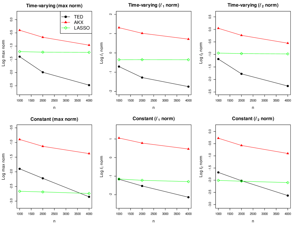
Figure 1: The log max, $\ell_{1}$, and $\ell_{2}$ norm error plots of the TED (black dot), AKX (red triangle), and LASSO (green diamond) estimators for $p=100$ and $n=1000,2000,4000$.

Figure 1 plots the log max, $\ell_{1}$, and $\ell_{2}$ norm errors of the TED, AKX, and LASSO estimators for the time-varying and constant beta processes with $p=100$ and $n=1000,2000,4000$. From Figure 1, we find that the estimation errors of the TED estimator are decreasing as the number of high-frequency observations increases. For the time-varying beta process, the TED estimator outperforms other estimators. This may be because the proposed TED estimation method can account for both time variation and the high-dimensionality of the beta process, while the AKX and LASSO estimators fail to explain one of them. When comparing the AKX and LASSO estimators, the LASSO estimator shows better performance. This may be because the errors from the curse of dimensionality are much more significant than those from the time-varying beta in this simulation study. For the constant beta process, the TED and LASSO estimators outperform the AKX estimator. This is probably due to the fact that only the AKX estimator is unable to handle the curse of dimensionality. From these results, we can conjecture that the TED estimator accounts for the time variation and high-dimensionality of the beta process and is robust to the beta process structure.

5 An empirical study

We applied the proposed TED estimator to real high-frequency trading data from January 2013 to December 2019. We took stock price data from the End of Day website (https://eoddata.com/), firm fundamentals from the Center for Research in Security Prices (CRSP)/Compustat Merged Database, and futures price data from the FirstRate Data website. For each stock and futures, we obtained 5-min log-price data using the previous tick scheme (Wang and Zou,, 2010; Zhang,, 2011), where the half trading days were excluded. We considered the log-prices of the five assets as the dependent processes. Specifically, we selected Apple Inc. (AAPL), Berkshire Hathaway Inc. (BRK.B), General Motors Company (GM), Alphabet Inc. (GOOG), and Exxon Mobil Corporation (XOM). These firms are the top market value stocks in five global industrial classification standards (GICS) sectors: information technology, financials, consumer discretionary, communication services, and energy sectors. For the covariate process, we collected the price data of 54 futures that represent market macro variables. For example, we selected 20 commodity data, 10 currency data, 10 interest rate data, and 14 stock market index data. We listed the symbols of 54 futures in Table 2 in the supplementary materials. Furthermore, we considered Fama-French five factors in Fama and French, (2015) and the momentum factor in Carhart, (1997). We denoted market, value, size, profitability, investment, and momentum factors by MKT, HML, SMB, RMW, CMA, and MOM, respectively. We constructed these factors with high-frequency data similar to the scheme in Aït-Sahalia et al., (2020) as follows. First, we obtained the monthly portfolio constituents for above six factors with the stocks listed on NYSE, NASDAQ, and AMEX. Specifically, the MKT is the return of a value-weighted portfolio of whole assets, while the other factors are as follows:

$$HML=\left(SH+BH\right)/2-\left(SL+BL\right)/2,$$

$$SMB=\left(SH+SM+SL\right)/3-\left(BH+BM+BL\right)/3,$$

$$RMW=\left(SR+BR\right)/2-\left(SW+BW\right)/2,$$

$$CMA=\left(SC+BC\right)/2-\left(SA+BA\right)/2,$$

$$MOM=\left(SU+BU\right)/2-\left(SD+BD\right)/2,$$

where small (S) and big (B) portfolios were classified by the market equity, while high (H), medium (M), and low (L) portfolios were classified by their ratio of book equity to market equity. Also, we classified robust (R), neutral (N), and weak (W) portfolios according to their profitability, while conservative (C), neutral (N), and aggressive (A) portfolios were classified by their investment. Finally, we classified up (U), flat (F), and down (D) portfolios according to the momentum of the return. The details of this process can be found in Aït-Sahalia et al., (2020). Then, we calculated each portfolio return with a frequency of five minutes using the portfolio weights adjusted at a five-minute frequency. Specifically, we obtained the return of any portfolios, $WRet_{d,i}$, for the $d$th day and $i$th time interval as follows:

$$WRet_{d,i}=\dfrac{\sum_{j=1}^{N_{d}}w_{d,i}^{j}\times Ret_{d,i}^{j}}{\sum_{j=1}^{N_{d}}w_{d,i}^{j}},$$

where $N_{d}$ is the number of stocks for the portfolio on the day $d$, the superscript $j$ represents the $j$th stock of the portfolio, and $w_{d,i}^{j}$ is obtained by

$$w_{d,i}^{j}=w_{d}^{j}\times\prod_{l=0}^{i-1}\left(1+Ret_{d,l}^{j}\right),$$

where $w_{d}^{j}$ is the market capitalization calculated using the close price of the $j$th stock on the day $d-1$, and $Ret_{d,0}^{j}$ is the overnight return from the $\left(d-1\right)$th day to the $d$th day. In sum, we utilized the five assets and 60 factors for the dependent processes and covariate processes, respectively.

For the choice of the tuning parameter $c_{h}$, we calculated the mean squared prediction error (MSPE) from the data in $2013$. Specifically, we first defined

$$\Lambda(c_{h})=\frac{1}{55}\sum_{j=1}^{5}\sum_{m=1}^{11}\left\|\widetilde{I\beta}^{m,j}\left(c_{h}\right)-\widehat{I\beta}^{(m+1),j}\right\|_{2}^{2},$$

where $\widetilde{I\beta}^{m,j}\left(c_{h}\right)$ is the TED estimator obtained using the tuning parameter $c_{h}$ and $\widehat{I\beta}^{m,j}$ is the debiased Dantzig integrated beta estimator for the $m$th month of $2013$ and $j$th stock. Then, we selected $c_{h}$ which minimizes $\Lambda(c_{h})$ over $c_{h}\in\left\{l/10\mid 0\leq l\leq 5,\,l\in\mathbb{Z}\right\}$. The result is $c_{h}=0.5$. We note that the stationarity assumption is reasonable for the beta process, which justifies the proposed tuning parameter choice procedure. Then, for each of the five assets, we employed the TED, AKX, and LASSO estimation procedures to obtain the monthly integrated betas. The tuning parameters were selected based on Section 3.4 and Section 4. Since the AKX estimator is designed for the finite dimension, we also employed the AKX-SIX estimator. The AKX-SIX estimator employs the same estimation method as the AKX estimator except that it only uses MKT, HML, SMB, RMW, CMA, and MOM as factor candidates. We note that these six factors are commonly used in finance practice (Asness et al.,, 2013; Barroso and Santa-Clara,, 2015; Carhart,, 1997; Fama and French,, 2015, 2016). For each estimation procedure, the betas for the non-trading period were estimated to be zero.

Table 1: The annual average in-sample and out-of-sample $R^{2}$ for the TED, AKX, AKX-SIX, and LASSO estimators across the five assets.

		In-sample $R^{2}$
		Estimator
		TED		AKX		AKX-SIX		LASSO
whole period		0.272		0.179		0.053		0.249
2013		0.237		0.163		0.038		0.232
2014		0.246		0.157		0.040		0.217
2015		0.305		0.220		0.067		0.286
2016		0.282		0.197		0.065		0.245
2017		0.211		0.086		0.017		0.180
2018		0.369		0.264		0.094		0.349
2019		0.256		0.170		0.047		0.236
		Out-of-sample $R^{2}$
		Estimator
		TED		AKX		AKX-SIX		LASSO
whole period		0.266		0.169		0.049		0.243
2014		0.239		0.144		0.034		0.211
2015		0.286		0.203		0.060		0.269
2016		0.267		0.190		0.063		0.240
2017		0.200		0.079		0.015		0.173
2018		0.353		0.234		0.069		0.341
2019		0.251		0.165		0.052		0.226

To investigate the performances of the TED, AKX, AKX-SIX, and LASSO estimators, we first calculated the monthly in-sample and out-of-sample $R^{2}$ from the monthly integrated beta estimates. We obtained the out-of-sample $R^{2}$ using the integrated beta estimates from the previous month. The out-of-sample $R^{2}$ was calculated from 2014 to 2019 since the tuning parameters were selected from the data in 2013. Then, we calculated the annual average $R^{2}$ over the five assets and twelve months. Table 1 reports the annual average in-sample and out-of-sample $R^{2}$ for the TED, AKX, AKX-SIX, and LASSO estimators. From Table 1, we can find that the high-dimensional regression models (TED and LASSO) show better performance than the finite-dimensional regression model. This may be because as we know, the high-dimensional models can overcome the curse of dimensionality. When comparing TED and LASSO, the TED estimator shows the best result for all periods. This is probably due to the fact that only the TED estimator can account for both the high-dimensionality and time-varying property of the beta process.

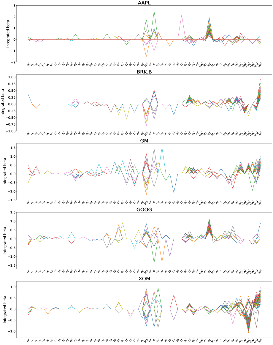
Figure 2: The monthly integrated betas from the TED estimation procedure for the five assets and 60 factors. Each line represents the integrated beta estimates for each month.

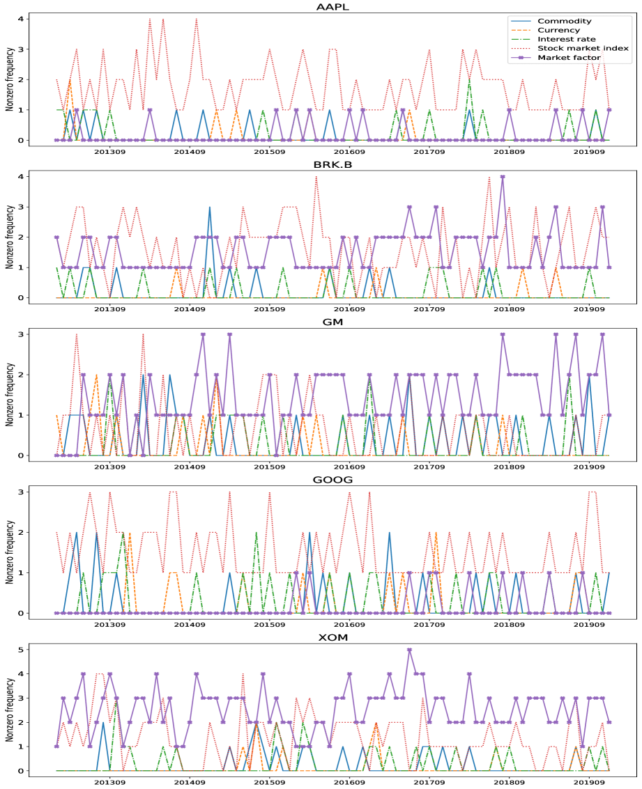
Figure 3: The nonzero frequency of the monthly integrated betas from the TED estimation procedure for the five assets and five groups. The five groups are the commodity futures group, currency futures group, interest rate futures group, stock market index futures group, and market factor group.

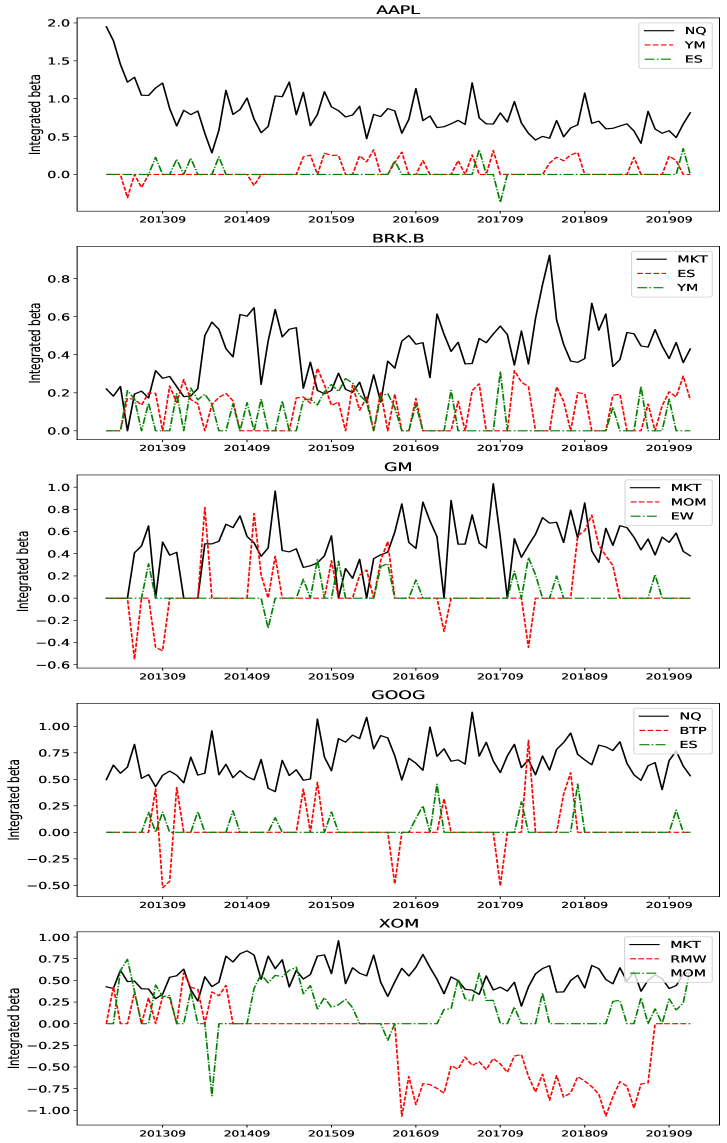
Figure 4: The integrated betas from the TED estimation procedure for the three most frequent factors among the 60 factors for each of the five assets.

Now, we investigate the TED estimation results. Figure 2 depicts the monthly integrated beta estimates for the five assets and 60 factors, and Figure 3 plots the nonzero frequency of monthly integrated betas for the five groups, such as the commodity futures group, currency futures group, interest rate futures group, stock market index futures group, and market factor group. From Figures 2–3, we find that the value of the integrated beta varies over time and the significant betas also change over time. Furthermore, the stock market index futures group had non-zero integrated beta estimates more often than the other futures groups. This may be because the stock market index futures can partially explain the market factors. This finding is consistent with the multi-factor models (Asness et al.,, 2013; Carhart,, 1997; Fama and French,, 1992, 2015). On the other hand, there are several individual factors that played a significant role in most periods. Thus, to investigate the beta behavior in greater details, we draw the integrated betas for the five assets and the three most frequent factors illustrated in Figure 4. For example, AAPL has NQ (E-mini Nasdaq-100), YM (E-mini Dow), and ES (E-mini S&P 500); BRK.B has MKT, ES, and YM; GM has MKT, MOM, and EW (E-mini S&P 500 Midcap); GOOG has NQ, BTP (Euro BTP Long-Bond), and ES; and XOM has MKT, RMW, and MOM. Among the factors, either the NQ factor or MKT factor is the most frequently significant factor. Moreover, the beta values of the three most frequent factors vary over time, while other factors are significant only for some periods. From these results, we can infer that the beta processes are sparse and time-varying. Hence, incorporating these features is important to account for market dynamics. The proposed TED procedure can provide a good tool to deal with these issues when analyzing market dynamics using high-frequency data.

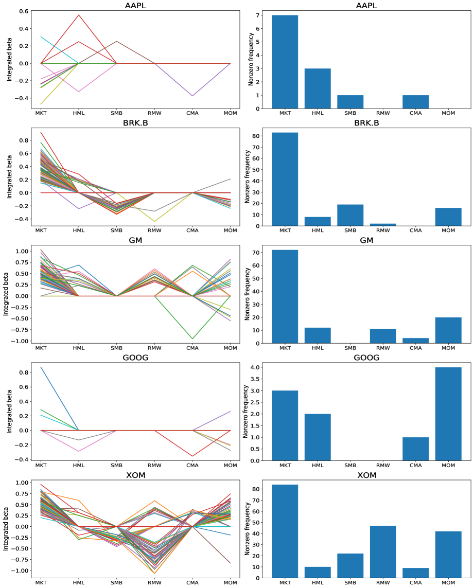
Figure 5: The integrated beta estimates from the TED estimation procedure (left) and the nonzero frequency (right) for the six factors, MKT, HML, SMB, RMW, CMA, and MOM. Each line (left) represents the integrated beta estimates for each month.

In finance practice, the six factors (Fama-French five factors and the momentum factor) are most frequently used (Asness et al.,, 2013; Barroso and Santa-Clara,, 2015; Carhart,, 1997; Fama and French,, 2015, 2016). Thus, we investigate their integrated beta behaviors. Figure 5 depicts the estimates of the monthly integrated beta for MKT, HML, SMB, RMW, CMA, and MOM with their non-zero frequency. We find that the MKT factor was significant for BRK.B, GM, and XOM, which may indicate that these firms can be adequately explained by the market movements. Other market factors are also significant for some periods; thus, these factors can explain expected stock returns for BRK.B, GM, and XOM. In contrast, for technology companies such as AAPL and GOOG, the integrated beta estimates for the MKT factor are usually small. This may be because the NQ (E-mini Nasdaq-100) factor played a significant role for the technology stocks as shown in Figure 4. Furthermore, AAPL and GOOG cannot be satisfactorily explained using the common six factors. One possible explanation is that, over the last twenty years, the technology companies have led the U.S. economy, with AAPL and GOOG as the most successful companies in the same time frame. Thus, these six factors may not work well for the period when we studied them.

6 Conclusion

In this paper, we proposed a novel Thresholding dEbiased Dantzig (TED) estimation procedure which can accommodate the sparse and time-varying beta process in the high-dimensional set-up. Specifically, to account for the sparse and time-varying beta process, we applied the Dantzig procedure to the instantaneous beta estimator, which results in a biased estimator. To reduce the bias, we proposed a debiased estimation procedure. We estimated the integrated beta with this new debiased instantaneous beta estimator. We showed that the Dantzig procedure can handle the sparsity of the instantaneous beta and that the debiased scheme mitigates the errors from the bias of the instantaneous beta estimator. To accommodate the sparsity of the integrated beta, we further regularized the beta estimator. Finally, we showed that the proposed TED estimator can obtain the near-optimal convergence rate.

In the empirical study, the TED estimator outperforms other estimators in terms of both in-sample and out-of-sample $R^{2}$. Furthermore, we found that the beta process is sparse and time-varying. These findings revealed that, when analyzing the high-dimensional high-frequency regression, the TED estimator is a useful tool which can handle the curse of dimensionality and the time-varying beta. That is, in practice, the TED procedure makes it possible to analyze the stock market with relatively short period using high-frequency data.

Funding

This work was supported by the National Research Foundation of Korea [2021R1C1C1003216].

Supplement to “High-Dimensional Time-Varying Coefficient Estimation”

Appendix A Proofs

A.1 Proofs of Theorems 1 and 2

Without loss of generality, it is enough to show the statements of Theorems 1 and 2 for fixed $i$.
Proof of Theorem 1. We denote the true instantaneous beta at time $i\Delta_{n}$ by $\boldsymbol{\beta}_{0}$. We have

$$\Delta_{i+k}^{n}Y = \int_{(i+k-1)\Delta_{n}}^{(i+k)\Delta_{n}}\boldsymbol{\beta}_{t}^{\top}d\mathbf{X}_{t}+\int_{(i+k-1)\Delta_{n}}^{(i+k)\Delta_{n}}dZ_{t}$$

$$= \boldsymbol{\beta}_{0}^{\top}\Delta_{i+k}^{n}\mathbf{X}+\Delta_{i+k}^{n}Z+\int_{(i+k-1)\Delta_{n}}^{(i+k)\Delta_{n}}(\boldsymbol{\beta}_{t}-\boldsymbol{\beta}_{0})^{\top}d\mathbf{X}_{t}.$$

Then, we have

$$\mathcal{Y}_{i}=\mathcal{X}_{i}\boldsymbol{\beta}_{0}+\mathcal{Z}_{i}+\mathcal{\widetilde{X}}_{i},$$

where

$$\mathcal{\widetilde{X}}_{i}=\begin{pmatrix}\int_{i\Delta_{n}}^{(i+1)\Delta_{n}}(\boldsymbol{\beta}_{t}-\boldsymbol{\beta}_{0})^{\top}d\mathbf{X}_{t}\\ \int_{(i+1)\Delta_{n}}^{(i+2)\Delta_{n}}(\boldsymbol{\beta}_{t}-\boldsymbol{\beta}_{0})^{\top}d\mathbf{X}_{t}\\ \vdots\\ \int_{(i+k_{n}-1)\Delta_{n}}^{(i+k_{n})\Delta_{n}}(\boldsymbol{\beta}_{t}-\boldsymbol{\beta}_{0})^{\top}d\mathbf{X}_{t}\end{pmatrix}.$$

Since the instantaneous volatility and drift processes are bounded, $\Delta_{i+k}^{n}Z$ and $\Delta_{i+k}^{n}X_{j}$ are sub-Gaussian. Then, similar to proofs of Theorem 1 (Kim and Wang,, 2016), we can show, for some large $C$,

$$P\left(\max_{1\leq j\leq p}\left|\frac{1}{k_{n}\Delta_{n}}\sum_{k=0}^{k_{n}}\Delta_{i+k}^{n}Z\Delta_{i+k}^{n}X_{j}\right|\geq C\sqrt{\log p/k_{n}}\right)\leq p^{-1-a},$$ (A.1)

where $X_{j}$ is the $j$th element of $\mathbf{X}$.

Consider $\frac{1}{k_{n}\Delta_{n}}\mathcal{X}_{i}^{\top}\mathcal{\widetilde{X}}_{i}$. There exist standard Brownian motions, $W_{mt}^{*}$ and $B_{it}^{*}$, such that

$$d\beta_{mt}=\mu_{\beta,mt}dt+\sqrt{\Sigma_{\beta,mmt}}dW_{mt}^{*}\quad\text{and}\quad dX_{it}=\mu_{it}dt+\sqrt{\Sigma_{iit}}dB_{it}^{*},$$

and let $\widetilde{X}_{mt}=\int_{i\Delta_{n}}^{t}(\beta_{ms}-\beta_{m0})dX_{ms}$. By Itô’s formula, we have

$$\int_{(i+k-1)\Delta_{n}}^{(i+k)\Delta_{n}}dX_{jt}\int_{(i+k-1)\Delta_{n}}^{(i+k)\Delta_{n}}(\beta_{mt}-\beta_{m0})dX_{mt}$$

$$=\int_{(i+k-1)\Delta_{n}}^{(i+k)\Delta_{n}}(\beta_{mt}-\beta_{m0})\Sigma_{jmt}dt$$

$$\quad+\int_{(i+k-1)\Delta_{n}}^{(i+k)\Delta_{n}}(\widetilde{X}_{mt}-\widetilde{X}_{m(i+k-1)\Delta_{n}})dX_{jt}+\int_{(i+k-1)\Delta_{n}}^{(i+k)\Delta_{n}}(X_{jt}-X_{j(i+k-1)\Delta_{n}})d\widetilde{X}_{mt}$$

$$=\int_{(i+k-1)\Delta_{n}}^{(i+k)\Delta_{n}}\int_{i\Delta_{n}}^{t}\sqrt{\Sigma_{\beta,mms}}dW_{ms}^{*}\Sigma_{jmt}dt+\int_{(i+k-1)\Delta_{n}}^{(i+k)\Delta_{n}}\int_{i\Delta_{n}}^{t}\mu_{\beta,ms}ds\Sigma_{jmt}dt$$

$$\quad+\int_{(i+k-1)\Delta_{n}}^{(i+k)\Delta_{n}}(\widetilde{X}_{mt}-\widetilde{X}_{m(i+k-1)\Delta_{n}})\sqrt{\Sigma_{jjt}}dB_{jt}^{*}+\int_{(i+k-1)\Delta_{n}}^{(i+k)\Delta_{n}}(\widetilde{X}_{mt}-\widetilde{X}_{m(i+k-1)\Delta_{n}})\mu_{jt}dt$$

$$\quad+\int_{(i+k-1)\Delta_{n}}^{(i+k)\Delta_{n}}(X_{jt}-X_{j(i+k-1)\Delta_{n}})\sqrt{\Sigma_{mmt}}(\beta_{mt}-\beta_{m0})dB_{mt}^{*}$$

$$\quad+\int_{(i+k-1)\Delta_{n}}^{(i+k)\Delta_{n}}(X_{jt}-X_{j(i+k-1)\Delta_{n}})(\beta_{mt}-\beta_{m0})\mu_{mt}dt$$

$$=M_{1km}+D_{1km}+M_{2km}+D_{2km}+M_{3km}+D_{3km}\text{ a.s.}$$

First, consider $D_{ikm}$’s. By Assumption 1(b)–(c), we have

$$\left|\frac{1}{k_{n}\Delta_{n}}\sum_{m=1}^{p}\sum_{k=1}^{k_{n}}D_{1km}\right|\leq Cs_{p}k_{n}\Delta_{n}\text{ a.s.}$$

For $D_{2km}$, by Assumption 1(b)–(c), the process $\sum_{m=1}^{p}|\beta_{mt}-\beta_{m0}|$ has the sub-Gaussian tail and $\sum_{m=1}^{p}\sqrt{\Sigma_{\beta,mmt}}\leq C\sum_{m=1}^{p}|\Sigma_{\beta,mmt}|^{\delta/2}\leq Cs_{p}$. Thus, we can show

$$P\left(\sup_{t\in[i\Delta_{n},\left(i+k_{n}\right)\Delta_{n}]}\sum_{m=1}^{p}|\beta_{mt}-\beta_{m0}|\geq Cs_{p}\sqrt{\Delta_{n}k_{n}\log p}\right)$$ (A.2)

$$\leq CP\left(\sum_{m=1}^{p}|\beta_{m\left(i+k_{n}\right)\Delta_{n}}-\beta_{m0}|\geq Cs_{p}\sqrt{\Delta_{n}k_{n}\log p}\right)$$ (A.3)

$$\leq p^{-3-a-c/c_{1}}.$$ (A.4)

Let

$$E=\left\{\sup_{t\in[i\Delta_{n},\left(i+k_{n}\right)\Delta_{n}]}\sum_{m=1}^{p}|\beta_{mt}-\beta_{m0}|\geq Cs_{p}\sqrt{\Delta_{n}k_{n}\log p}\right\}.$$

Then, we have

$$P\left(\sup_{t\in[(i+k-1)\Delta_{n},(i+k)\Delta_{n}]}\sum_{m=1}^{p}|\widetilde{X}_{mt}-\widetilde{X}_{m(i+k-1)\Delta_{n}}|\geq Cs_{p}\log p\sqrt{\Delta_{n}^{2}k_{n}}\right)$$

$$\leq CP\left(\sum_{m=1}^{p}|\widetilde{X}_{m(i+k)\Delta_{n}}-\widetilde{X}_{m(i+k-1)\Delta_{n}}|\geq Cs_{p}\log p\sqrt{\Delta_{n}^{2}k_{n}}\right)$$

$$\leq CP\left(\sum_{m=1}^{p}\left|\int_{(i+k-1)\Delta_{n}}^{(i+k)\Delta_{n}}(\beta_{mt}-\beta_{m0})dX_{mt}\right|\geq Cs_{p}\log p\sqrt{\Delta_{n}^{2}k_{n}},E^{c}\right)+p^{-3-a-c/c_{1}}$$

$$\leq Cp^{-3-a-c/c_{1}},$$

which implies

$$P(\sup_{1\leq k\leq k_{n}}\sup_{t\in[(i+k-1)\Delta_{n},(i+k)\Delta_{n}]}\sum_{m=1}^{p}|\widetilde{X}_{mt}-\widetilde{X}_{m(i+k-1)\Delta_{n}}|\geq Cs_{p}\log p\sqrt{\Delta_{n}^{2}k_{n}})\leq Cp^{-3-a}.$$ (A.5)

Thus, we have, with probability at least $1-p^{-2-a}$,

$$\left|\frac{1}{k_{n}\Delta_{n}}\sum_{m=1}^{p}\sum_{k=1}^{k_{n}}D_{2km}\right|\leq Cs_{p}\log p\sqrt{\Delta_{n}^{2}k_{n}}.$$

Similarly, we can show, with probability at least $1-p^{-2-a}$,

$$\left|\frac{1}{k_{n}\Delta_{n}}\sum_{m=1}^{p}\sum_{k=1}^{k_{n}}D_{3km}\right|\leq Cs_{p}\log p\sqrt{\Delta_{n}^{2}k_{n}}.$$

Consider $M_{ikm}$’s. By Azuma-Hoeffding inequality, we have, with probability at least $1-p^{-2-a}$,

$$\left|\frac{1}{k_{n}\Delta_{n}}\sum_{m=1}^{p}\sum_{k=1}^{k_{n}}M_{1km}\right|\leq Cs_{p}\sqrt{\Delta_{n}k_{n}\log p}.$$

For $M_{2km}$, let

$$\eta_{mt}=(\widetilde{X}_{mt}-\widetilde{X}_{m(i+k-1)\Delta_{n}})\sqrt{\Sigma_{jjt}}\quad\text{ and }\quad Q_{t}=\boldsymbol{1}_{\{\sum_{m=1}^{p}|\eta_{mt}|\leq Cs_{p}\log p\sqrt{\Delta_{n}^{2}k_{n}}\}}.$$

Then, by Azuma-Hoeffding inequality, we have, with probability at least $1-p^{-3-a}$,

$$\left|\frac{1}{k_{n}\Delta_{n}}\sum_{m=1}^{p}\sum_{k=1}^{k_{n}}\int_{(i+k-1)\Delta_{n}}^{(i+k)\Delta_{n}}\eta_{mt}Q_{t}dB_{jt}^{*}\right|\leq Cs_{p}\sqrt{\Delta_{n}}(\log p)^{3/2}.$$

Thus, by (A.5), we have, with probability at least $1-p^{-2-a}$,

$$\left|\frac{1}{k_{n}\Delta_{n}}\sum_{m=1}^{p}\sum_{k=1}^{k_{n}}M_{2km}\right|\leq Cs_{p}\sqrt{\Delta_{n}}(\log p)^{3/2}.$$

Similarly, we can show, with probability at least $1-p^{-2-a}$,

$$\left|\frac{1}{k_{n}\Delta_{n}}\sum_{m=1}^{p}\sum_{k=1}^{k_{n}}M_{3km}\right|\leq Cs_{p}\sqrt{\Delta_{n}}(\log p)^{3/2}.$$

Therefore, we have, with probability at least $1-Cp^{-1-a}$,

$$\max_{1\leq j\leq p}\left|\frac{1}{k_{n}\Delta_{n}}\sum_{k=1}^{k_{n}}\Delta_{i+k}^{n}X_{j}\int_{(i+k-1)\Delta_{n}}^{(i+k)\Delta_{n}}(\boldsymbol{\beta}_{t}-\boldsymbol{\beta}_{0})^{\top}d\mathbf{X}_{t}\right|$$ (A.6)

$$\leq Cs_{p}\sqrt{\Delta_{n}k_{n}\log p}.$$ (A.7)

With probability greater than $1-p^{-1-a}$, we have

$$\left\|\frac{d}{dt}[\mathbf{X},\mathbf{X}]_{i\Delta_{n}}-\frac{1}{k_{n}\Delta_{n}}\mathcal{X}_{i}^{\top}\mathcal{X}_{i}\right\|_{\max} \leq \left\|\boldsymbol{\Sigma}_{i\Delta_{n}}-\frac{1}{k_{n}\Delta_{n}}\int_{i\Delta_{n}}^{\left(i+k_{n}\right)\Delta_{n}}\boldsymbol{\Sigma}_{s}ds\right\|_{\max}$$ (A.9)

$$+\left\|\frac{1}{k_{n}\Delta_{n}}\int_{i\Delta_{n}}^{\left(i+k_{n}\right)\Delta_{n}}\boldsymbol{\Sigma}_{s}ds-\frac{1}{k_{n}\Delta_{n}}\mathcal{X}_{i}^{\top}\mathcal{X}_{i}\right\|_{\max}$$

$$\leq C\sqrt{k_{n}\Delta_{n}}+C\sqrt{\log p/k_{n}},$$ (A.10)

where $\frac{d}{dt}[\mathbf{X},\mathbf{X}]_{t}=\boldsymbol{\Sigma}_{t}$ and the last inequality can be showed similar to the proofs of Theorem 1 (Kim and Wang,, 2016). Thus, by (A.1), (A.6), and (A.9), we show the statement under the following statements:

$$\left\|\frac{1}{k_{n}\Delta_{n}}\mathcal{X}_{i}^{\top}\mathcal{Z}_{i}\right\|_{\max}\leq C\sqrt{\log p/k_{n}},$$ (A.11)

$$\left\|\frac{1}{k_{n}\Delta_{n}}\mathcal{X}_{i}^{\top}\mathcal{\widetilde{X}}_{i}\right\|_{\max}\leq Cs_{p}\sqrt{k_{n}\Delta_{n}}\sqrt{\log p},$$ (A.12)

$$\left\|\frac{d}{dt}[\mathbf{X},\mathbf{X}]_{i\Delta_{n}}-\frac{1}{k_{n}\Delta_{n}}\mathcal{X}_{i}^{\top}\mathcal{X}_{i}\right\|_{\max}\leq C(\sqrt{k_{n}\Delta_{n}}+\sqrt{\log p/k_{n}}).$$ (A.13)

By (A.11), we have, for some large $C_{\lambda,a}$,

$$\left\|\frac{1}{k_{n}\Delta_{n}}\mathcal{X}_{i}^{\top}\mathcal{X}_{i}\boldsymbol{\beta}_{0}-\frac{1}{k_{n}\Delta_{n}}\mathcal{X}_{i}^{\top}\mathcal{Y}_{i}\right\|_{\max}$$

$$=\left\|\frac{1}{k_{n}\Delta_{n}}\mathcal{X}_{i}^{\top}\mathcal{X}_{i}\boldsymbol{\beta}_{0}-\frac{1}{k_{n}\Delta_{n}}\mathcal{X}_{i}^{\top}\mathcal{X}_{i}\boldsymbol{\beta}_{0}-\frac{1}{k_{n}\Delta_{n}}\mathcal{X}_{i}^{\top}\mathcal{Z}_{i}-\frac{1}{k_{n}\Delta_{n}}\mathcal{X}_{i}^{\top}\mathcal{\widetilde{X}}_{i}\right\|_{\max}$$

$$\leq\left\|\frac{1}{k_{n}\Delta_{n}}\mathcal{X}_{i}^{\top}\mathcal{Z}_{i}\right\|_{\max}+\left\|\frac{1}{k_{n}\Delta_{n}}\mathcal{X}_{i}^{\top}\mathcal{\widetilde{X}}_{i}\right\|_{\max}$$

$$\leq\lambda_{n}.$$

Thus, $\boldsymbol{\beta}_{0}$ satisfies the constraint in (3.2), which implies that

$$\|\widehat{\boldsymbol{\beta}}_{i\Delta_{n}}\|_{1}\leq\|\boldsymbol{\beta}_{0}\|_{1}.$$

We have

$$\|\frac{1}{k_{n}\Delta_{n}}\mathcal{X}_{i}^{\top}\mathcal{X}_{i}(\widehat{\boldsymbol{\beta}}_{i\Delta_{n}}-\boldsymbol{\beta}_{0})\|_{\max} \leq \|\frac{1}{k_{n}\Delta_{n}}\mathcal{X}_{i}^{\top}\mathcal{X}_{i}\widehat{\boldsymbol{\beta}}_{i\Delta_{n}}-\frac{1}{k_{n}\Delta_{n}}\mathcal{X}_{i}^{\top}\mathcal{Y}_{i}\|_{\max}$$

$$+\|\frac{1}{k_{n}\Delta_{n}}\mathcal{X}_{i}^{\top}\mathcal{X}_{i}\boldsymbol{\beta}_{0}-\frac{1}{k_{n}\Delta_{n}}\mathcal{X}_{i}^{\top}\mathcal{Y}_{i}\|_{\max}$$

$$\leq 2\lambda_{n}$$

and

$$\|\boldsymbol{\Sigma}_{i\Delta_{n}}(\widehat{\boldsymbol{\beta}}_{i\Delta_{n}}-\boldsymbol{\beta}_{0})\|_{\max} \leq \|\frac{1}{k_{n}\Delta_{n}}\mathcal{X}_{i}^{\top}\mathcal{X}_{i}(\widehat{\boldsymbol{\beta}}_{i\Delta_{n}}-\boldsymbol{\beta}_{0})\|_{\max}$$

$$+\|(\boldsymbol{\Sigma}_{i\Delta_{n}}-\frac{1}{k_{n}\Delta_{n}}\mathcal{X}_{i}^{\top}\mathcal{X}_{i})(\widehat{\boldsymbol{\beta}}_{i\Delta_{n}}-\boldsymbol{\beta}_{0})\|_{\max}$$

$$\leq 2\lambda_{n}+2\|\boldsymbol{\beta}_{0}\|_{1}\|\boldsymbol{\Sigma}_{i\Delta_{n}}-\frac{1}{k_{n}\Delta_{n}}\mathcal{X}_{i}^{\top}\mathcal{X}_{i}\|_{\max}$$

$$\leq 2\lambda_{n}+Cs_{p}(\sqrt{k_{n}\Delta_{n}}+\sqrt{\log p/k_{n}})$$

$$\leq C\lambda_{n},$$

where the third inequality is due to (A.11) and the sparsity condition (2.3). Then, we have

$$\|\widehat{\boldsymbol{\beta}}_{i\Delta_{n}}-\boldsymbol{\beta}_{0}\|_{\max} \leq \|\boldsymbol{\Sigma}_{i\Delta_{n}}^{-1}\|_{1}\|\boldsymbol{\Sigma}_{i\Delta_{n}}(\widehat{\boldsymbol{\beta}}_{i\Delta_{n}}-\boldsymbol{\beta}_{0})\|_{\max}$$

$$\leq C\lambda_{n},$$

where the last inequality is due to Assumption 1(b).

Now, we consider the $\ell_{1}$ norm error bound. Let $a_{n}=\|\widehat{\boldsymbol{\beta}}_{i\Delta_{n}}-\boldsymbol{\beta}_{0}\|_{\max}$. Define

$$A=\widehat{\boldsymbol{\beta}}_{i\Delta_{n}}-\boldsymbol{\beta}_{0},$$

$$A_{1}=\left(\widehat{\beta}_{ji\Delta_{n}}1(|\widehat{\beta}_{ji\Delta_{n}}|\geq 2a_{n});1\leq j\leq p\right)^{\top}-\boldsymbol{\beta}_{0}.$$

Then, we have

$$\|\boldsymbol{\beta}_{0}\|_{1}-\|A_{1}\|_{1}+\|A-A_{1}\|_{1}\leq\|A_{1}+\boldsymbol{\beta}_{0}\|_{1}+\|A-A_{1}\|_{1}=\|\widehat{\boldsymbol{\beta}}_{i\Delta_{n}}\|_{1}\leq\|\boldsymbol{\beta}_{0}\|_{1},$$

which implies

$$\|A\|_{1}\leq\|A-A_{1}\|_{1}+\|A_{1}\|_{1}\leq 2\|A_{1}\|_{1}.$$

Therefore, it is enough to investigate the convergence rate of $\|A_{1}\|_{1}$. We have

$$\|A_{1}\|_{1} = \sum_{j=1}^{p}|\widehat{\beta}_{ji\Delta_{n}}1(|\widehat{\beta}_{ji\Delta_{n}}|\geq 2a_{n})-\beta_{j0}|$$ (A.14)

$$\leq \sum_{j=1}^{p}|\widehat{\beta}_{ji\Delta_{n}}1(|\widehat{\beta}_{ji\Delta_{n}}|\geq 2a_{n})-\beta_{j0}1(|\beta_{j0}|\geq 2a_{n})|+\sum_{j=1}^{p}|\beta_{j0}|1(|\beta_{j0}|\leq 2a_{n})$$ (A.15)

$$\leq \sum_{j=1}^{p}|\widehat{\beta}_{ji\Delta_{n}}1(|\widehat{\beta}_{ji\Delta_{n}}|\geq 2a_{n})-\beta_{j0}1(|\beta_{j0}|\geq 2a_{n})|+Cs_{p}a_{n}^{1-\delta}$$ (A.16)

$$\leq a_{n}\sum_{j=1}^{p}1(|\widehat{\beta}_{ji\Delta_{n}}|\geq 2a_{n})+\sum_{j=1}^{p}|\beta_{j0}||1(|\beta_{j0}|\geq 2a_{n})-1(|\widehat{\beta}_{ji\Delta_{n}}|\geq 2a_{n})|+Cs_{p}a_{n}^{1-\delta}$$ (A.17)

$$\leq a_{n}\sum_{j=1}^{p}1(|\beta_{j0}|\geq a_{n})+\sum_{j=1}^{p}|\beta_{j0}||1(|\beta_{j0}|\geq 2a_{n})-1(|\widehat{\beta}_{ji\Delta_{n}}|\geq 2a_{n})|+Cs_{p}a_{n}^{1-\delta}$$ (A.18)

$$\leq \sum_{j=1}^{p}|\beta_{j0}||1(|\beta_{j0}|\geq 2a_{n})-1(|\widehat{\beta}_{ji\Delta_{n}}|\geq 2a_{n})|+Cs_{p}a_{n}^{1-\delta}$$ (A.19)

$$\leq \sum_{j=1}^{p}|\beta_{j0}|1(||\beta_{j0}|-2a_{n}|\leq||\beta_{j0}|-|\widehat{\beta}_{ji\Delta_{n}}||)+Cs_{p}a_{n}^{1-\delta}$$ (A.20)

$$\leq \sum_{j=1}^{p}|\beta_{j0}|1(|\beta_{j0}|\leq 3a_{n})+Cs_{p}a_{n}^{1-\delta}$$ (A.21)

$$\leq Cs_{p}a_{n}^{1-\delta}.$$ (A.22)

$\blacksquare$

Proof of Theorem 2.

We denote the inverse matrix of the true instantaneous volatility matrix at time $i\Delta_{n}$ by $\boldsymbol{\Omega}_{0}$. By (A.9), we have, with probability greater than $1-p^{-1-a}$,

$$\left\|\frac{1}{k_{n}\Delta_{n}}\mathcal{X}_{i}^{\top}\mathcal{X}_{i}\boldsymbol{\Omega}_{0}-\mathbf{I}\right\|_{\max} = \left\|\left(\frac{1}{k_{n}\Delta_{n}}\mathcal{X}_{i}^{\top}\mathcal{X}_{i}-\frac{d}{dt}[\mathbf{X},\mathbf{X}]_{i\Delta_{n}}\right)\boldsymbol{\Omega}_{0}\right\|_{\max}$$

$$\leq \left\|\boldsymbol{\Omega}_{0}\right\|_{1}\left\|\left(\frac{1}{k_{n}\Delta_{n}}\mathcal{X}_{i}^{\top}\mathcal{X}_{i}-\frac{d}{dt}[\mathbf{X},\mathbf{X}]_{i\Delta_{n}}\right)\right\|_{\max}$$

$$\leq C(\sqrt{k_{n}\Delta_{n}}+\sqrt{\log p/k_{n}}).$$

Thus, by the constraint in (3.3), we have

$$P\left(\left\|\widehat{\boldsymbol{\Omega}}_{i\Delta_{n}}\right\|_{1}\leq C\right)\geq 1-p^{-1-a}.$$ (A.23)

Then, similar to the proofs of Theorem 1, we can show the statement. $\blacksquare$

A.2 Proof of Theorem 3

Proof of Theorem 3. Consider (3.7) and (3.8). Without loss of generality, it is enough to show (3.7) and (3.8) for fixed $i$. We have

$$\widetilde{\boldsymbol{\beta}}_{i\Delta_{n}}-\boldsymbol{\beta}_{0,i\Delta_{n}} = \frac{1}{k_{n}\Delta_{n}}\boldsymbol{\Omega}_{0,i\Delta_{n}}\mathcal{X}_{i}^{\top}\mathcal{Z}_{i}+\frac{1}{k_{n}\Delta_{n}}\widehat{\boldsymbol{\Omega}}_{i\Delta_{n}}^{\top}\mathcal{X}_{i}^{\top}\mathcal{\widetilde{X}}_{i}$$

$$-\left(\frac{1}{k_{n}\Delta_{n}}\widehat{\boldsymbol{\Omega}}_{i\Delta_{n}}^{\top}\mathcal{X}_{i}^{\top}\mathcal{X}_{i}-\mathbf{I}\right)(\widehat{\boldsymbol{\beta}}_{i\Delta_{n}}-\boldsymbol{\beta}_{0,i\Delta_{n}})+\frac{1}{k_{n}\Delta_{n}}(\widehat{\boldsymbol{\Omega}}_{i\Delta_{n}}^{\top}-\boldsymbol{\Omega}_{0,i\Delta_{n}})\mathcal{X}_{i}^{\top}\mathcal{Z}_{i}.$$

For $\frac{1}{k_{n}\Delta_{n}}\widehat{\boldsymbol{\Omega}}_{i\Delta_{n}}\mathcal{X}_{i}^{\top}\mathcal{\widetilde{X}}_{i}$, by the proofs of (A.6), we have

$$\frac{1}{k_{n}\Delta_{n}}\boldsymbol{\Omega}_{0,i\Delta_{n}}\mathcal{X}_{i}^{\top}\mathcal{\widetilde{X}}_{i}=\frac{1}{k_{n}\Delta_{n}}\boldsymbol{\Omega}_{0,i\Delta_{n}}\mathcal{A}_{i}+R_{X,i},$$

where $\|R_{X,i}\|_{\max}\leq Cs_{p}(\log p)^{3/2}\sqrt{\Delta_{n}}$ with probability greater than $1-Cp^{-1-a}$, and

$$\mathcal{A}_{i}=\left(\sum_{m=1}^{p}\int_{i\Delta_{n}}^{\left(i+k_{n}\right)\Delta_{n}}\int_{i\Delta_{n}}^{t}\sqrt{\Sigma_{\beta,mms}}dW_{ms}^{*}\Sigma_{jmt}dt\right)_{j=1,\ldots,p}.$$ (A.24)

By Theorem 2 and (A.6), we have, with probability greater than $1-Cp^{-1-a}$,

$$\left\|\frac{1}{k_{n}\Delta_{n}}\left(\boldsymbol{\Omega}_{0,i\Delta_{n}}-\widehat{\boldsymbol{\Omega}}_{i\Delta_{n}}^{\top}\right)\mathcal{X}_{i}^{\top}\mathcal{\widetilde{X}}_{i}\right\|_{\max}\leq Cs_{\omega,p}s_{p}\left(\sqrt{\log p/n^{1/2}}\right)^{2-q}.$$

Thus, we have, with probability greater than $1-Cp^{-1-a}$,

$$\frac{1}{k_{n}\Delta_{n}}\widehat{\boldsymbol{\Omega}}_{i\Delta_{n}}^{\top}\mathcal{X}_{i}^{\top}\mathcal{\widetilde{X}}_{i}=\frac{1}{k_{n}\Delta_{n}}\boldsymbol{\Omega}_{0,i\Delta_{n}}\mathcal{A}_{i}+R_{X,i}^{{}^{\prime}},$$ (A.25)

where $\|R_{X,i}^{{}^{\prime}}\|_{\max}\leq C\left\{s_{\omega,p}s_{p}\left(\sqrt{\log p/n^{1/2}}\right)^{2-q}+s_{p}(\log p)^{3/2}\sqrt{\Delta_{n}}\right\}$.

For $\left(\frac{1}{k_{n}\Delta_{n}}\widehat{\boldsymbol{\Omega}}_{i\Delta_{n}}^{\top}\mathcal{X}_{i}^{\top}\mathcal{X}_{i}-\mathbf{I}\right)(\widehat{\boldsymbol{\beta}}_{i\Delta_{n}}-\boldsymbol{\beta}_{0,i\Delta_{n}})$, we have, with probability greater than $1-p^{-1-a}$,

$$\|\left(\frac{1}{k_{n}\Delta_{n}}\widehat{\boldsymbol{\Omega}}_{i\Delta_{n}}^{\top}\mathcal{X}_{i}^{\top}\mathcal{X}_{i}-\mathbf{I}\right)(\widehat{\boldsymbol{\beta}}_{i\Delta_{n}}-\boldsymbol{\beta}_{0,i\Delta_{n}})\|_{\max}$$ (A.26)

$$\leq\|\frac{1}{k_{n}\Delta_{n}}\widehat{\boldsymbol{\Omega}}_{i\Delta_{n}}^{\top}\mathcal{X}_{i}^{\top}\mathcal{X}_{i}-\mathbf{I}\|_{\max}\|\widehat{\boldsymbol{\beta}}_{i\Delta_{n}}-\boldsymbol{\beta}_{0,i\Delta_{n}}\|_{1}$$ (A.27)

$$\leq C\tau_{n}s_{p}\lambda_{n}^{1-\delta}$$ (A.28)

$$\leq Cs_{p}^{2-\delta}(\log p)^{1-\delta/2}\left(\sqrt{k_{n}\Delta_{n}}+k_{n}^{-1/2}\right)^{2-\delta},$$ (A.29)

where the second inequality is by Theorem 1 and (3.3). For the last term, we have

$$\|\frac{1}{k_{n}\Delta_{n}}(\widehat{\boldsymbol{\Omega}}_{i\Delta_{n}}^{\top}-\boldsymbol{\Omega}_{0,i\Delta_{n}})\mathcal{X}_{i}^{\top}\mathcal{Z}_{i}\|_{\max} \leq \|\widehat{\boldsymbol{\Omega}}_{i\Delta_{n}}^{\top}-\boldsymbol{\Omega}_{0,i\Delta_{n}}\|_{\infty}\|\frac{1}{k_{n}\Delta_{n}}\mathcal{X}_{i}^{\top}\mathcal{Z}_{i}\|_{\max}$$ (A.30)

$$\leq Cs_{\omega,p}\tau_{n}^{1-q}\sqrt{\log p/k_{n}}$$ (A.31)

$$\leq Cs_{\omega,p}(\log p)^{1-q/2}(\sqrt{k_{n}\Delta_{n}}+k_{n}^{-1/2})^{1-q}k_{n}^{-1/2},$$ (A.32)

where the second inequality is due to Theorem 2 and (A.1), with probability greater than $1-Cp^{-1-a}$. By (A.25), (A.26), and (A.30), we have, with probability greater than $1-p^{-a}$,

$$\widetilde{\boldsymbol{\beta}}_{i\Delta_{n}}-\boldsymbol{\beta}_{0,i\Delta_{n}}=\frac{1}{k_{n}\Delta_{n}}\boldsymbol{\Omega}_{0,i\Delta_{n}}\left(\mathcal{X}_{i}^{\top}\mathcal{Z}_{i}+\mathcal{A}_{i}\right)+R_{i},$$ (A.33)

where

$$\|R_{i}\|_{\max}\leq C\left\{s_{p}^{2-\delta}(\log p/n^{1/2})^{(2-\delta)/2}+s_{p}s_{\omega,p}(\log p/n^{1/2})^{(2-q)/2}+s_{p}(\log p)^{3/2}/n^{1/2}\right\}.$$

Consider (3.9). We have

$$\widehat{I\beta}-I\beta_{0} = k_{n}\Delta_{n}\sum_{i=0}^{[1/(k_{n}\Delta_{n})]-1}\left(\widetilde{\boldsymbol{\beta}}_{ik_{n}\Delta_{n}}-\boldsymbol{\beta}_{0,ik_{n}\Delta_{n}}\right)$$

$$+\sum_{i=0}^{[1/(k_{n}\Delta_{n})]-1}\int_{ik_{n}\Delta_{n}}^{(i+1)k_{n}\Delta_{n}}(\boldsymbol{\beta}_{0,ik_{n}\Delta_{n}}-\boldsymbol{\beta}_{0,t})dt-\int_{[1/(k_{n}\Delta_{n})]k_{n}\Delta_{n}}^{1}\boldsymbol{\beta}_{0,t}dt.$$

First, we consider the discretization error terms. Since the beta process has the sub-Gaussian tail, we can show, with probability greater than $1-p^{-1-a}$,

$$\left\|\sum_{i=0}^{[1/(k_{n}\Delta_{n})]-1}\int_{ik_{n}\Delta_{n}}^{(i+1)k_{n}\Delta_{n}}(\boldsymbol{\beta}_{0,ik_{n}\Delta_{n}}-\boldsymbol{\beta}_{0,t})dt\right\|_{\max}\leq C\sqrt{\log p/n}.$$

Also, by Assumption 1(b), we have

$$\left\|\int_{[1/(k_{n}\Delta_{n})]k_{n}\Delta_{n}}^{1}\boldsymbol{\beta}_{0,t}dt\right\|_{\max}\leq Cn^{-1/2}\text{ a.s.}$$

Consider $\sum_{i=0}^{[1/(k_{n}\Delta_{n})]-1}\left(\widetilde{\boldsymbol{\beta}}_{ik_{n}\Delta_{n}}-\boldsymbol{\beta}_{0,ik_{n}\Delta_{n}}\right)$. By (3.7), we have

$$\sum_{i=0}^{[1/(k_{n}\Delta_{n})]-1}\left(\widetilde{\boldsymbol{\beta}}_{ik_{n}\Delta_{n}}-\boldsymbol{\beta}_{0,ik_{n}\Delta_{n}}\right)=\sum_{i=0}^{[1/(k_{n}\Delta_{n})]-1}\frac{1}{k_{n}\Delta_{n}}\boldsymbol{\Omega}_{0,ik_{n}\Delta_{n}}\left(\mathcal{X}_{ik_{n}}^{\top}\mathcal{Z}_{ik_{n}}+\mathcal{A}_{ik_{n}}\right)+R_{ik_{n}},$$

and, similar to the proofs of (A.33), we can show, with probability greater than $1-p^{-1-a}$,

$$\left\|\sum_{i=0}^{[1/(k_{n}\Delta_{n})]-1}R_{ik_{n}}\right\|_{\max}\leq\sum_{i=0}^{[1/(k_{n}\Delta_{n})]-1}\left\|R_{ik_{n}}\right\|_{\max}$$

$$\leq C\frac{1}{k_{n}\Delta_{n}}\left\{s_{p}^{2-\delta}(\log p/n^{1/2})^{(2-\delta)/2}+s_{p}s_{\omega,p}(\log p/n^{1/2})^{(2-q)/2}+s_{p}(\log p)^{3/2}/n^{1/2}\right\}.$$

Since the inverse matrix process $\boldsymbol{\Omega}_{0,ik_{n}\Delta_{n}}$ is bounded and $\mathcal{X}$ and $\mathcal{Z}$ have sub-Gaussian tails, similar to the proofs of Theorem 1 (Kim and Wang,, 2016), we can show, with probability greater than $1-p^{-1-a}$,

$$\left\|\sum_{i=0}^{[1/(k_{n}\Delta_{n})]-1}\boldsymbol{\Omega}_{0,ik_{n}\Delta_{n}}\mathcal{X}_{ik_{n}}^{\top}\mathcal{Z}_{ik_{n}}\right\|_{\max}\leq C\sqrt{\log p/n}.$$

Finally, we consider $\boldsymbol{\Omega}_{0,ik_{n}\Delta_{n}}\mathcal{A}_{ik_{n}}$ terms. Note that $\mathcal{A}_{ik_{n}}$’s are martingales with sub-Gaussian tails. Thus, by Azuma-Hoeffding inequality, we have, with probability greater than $1-p^{-1-a}$,

$$\|\sum_{i=0}^{[1/(k_{n}\Delta_{n})]-1}\boldsymbol{\Omega}_{0,ik_{n}\Delta_{n}}\mathcal{A}_{ik_{n}}\|_{\max}\leq Cs_{p}\sqrt{\log p}n^{-1/2}.$$

Therefore, the statement (3.9) is showed. $\blacksquare$

A.3 Proof of Theorem 4

Proof of Theorem 4. By (3.9), we can find $h_{n}$ such that, with probability greater than $1-p^{-a}$,

$$\|\widehat{I\beta}-I\beta_{0}\|_{\max}\leq h_{n}/2.$$ (A.34)

We show the statement under the event (A.34). Similar to the proof of (A.14), we can show

$$\|\widetilde{I\beta}-I\beta_{0}\|_{1}\leq Cs_{p}h_{n}^{1-\delta}.$$

$\blacksquare$

A.4 Proof of Theorem 5

Proof of Theorem 5. Define

$$\mathcal{Y}_{i}^{c}=\begin{pmatrix}\Delta_{i+1}^{n}Y^{c}\\ \Delta_{i+2}^{n}Y^{c}\\ \vdots\\ \Delta_{i+k_{n}}^{n}Y^{c}\end{pmatrix}\quad\text{and}\quad\mathcal{X}_{i}^{c}=\begin{pmatrix}\Delta_{i+1}^{n}\mathbf{X}^{c\top}\\ \Delta_{i+2}^{n}\mathbf{X}^{c\top}\\ \vdots\\ \Delta_{i+k_{n}}^{n}\mathbf{X}^{c\top}\end{pmatrix}.$$

For some large constant $C>0$, let

$$E_{1}=\left\{\max_{i,j}|\Delta_{i}^{n}X_{j}^{c}|\leq C\sqrt{\log p}n^{-1/2}\right\}\cap\left\{\max_{i,j}|\Delta_{i}^{n}Y_{j}^{c}|\leq Cs_{p}\sqrt{\log p}n^{-1/2}\right\},$$

$$E_{2}=\left\{\max_{i,j}\sum_{k=1}^{k_{n}}\boldsymbol{1}_{\{|\Delta_{i+k}^{n}X_{j}|>v_{j,n}\}}\leq C\log p\right\}\cap\left\{\max_{i,j}\int_{i\Delta_{n}}^{\left(i+k_{n}\right)\Delta_{n}}d\Lambda_{jt}\leq C\log p\right\}.$$

By the boundedness condition Assumption 1(b) and sparsity condition (2.3), we can show

$$P\left(E_{1}\right)\geq 1-p^{-2-a}.$$

Under the event $E_{1}$, we have, for large $n$,

$$\max_{i,j}\sum_{k=1}^{k_{n}}\boldsymbol{1}_{\{|\Delta_{i+k}^{n}X_{j}|>v_{j,n}\}}\leq\max_{i,j}\int_{i\Delta_{n}}^{\left(i+k_{n}\right)\Delta_{n}}d\Lambda_{jt},$$

where $\int_{i\Delta_{n}}^{\left(i+k_{n}\right)\Delta_{n}}d\Lambda_{jt}$ is a Poisson with the intensity $Ck_{n}\Delta_{n}$ for some constant $C>0$, and

$$P\left(\max_{i,j}\int_{i\Delta_{n}}^{\left(i+k_{n}\right)\Delta_{n}}d\Lambda_{jt}\geq C\log p\right)\leq p^{-2-a}.$$

Thus, we have

$$P\left(E_{1}\cap E_{2}\right)\geq 1-p^{-1-a}.$$ (A.35)

We have

$$\sum_{k=1}^{k_{n}}\Delta_{i+k}^{n}X_{j}\,\boldsymbol{1}_{\{|\Delta_{i+k}^{n}X_{j}|\leq v_{j,n}\}}\Delta_{i+k}^{n}X_{l}\,\boldsymbol{1}_{\{|\Delta_{i+k}^{n}X_{l}|\leq v_{l,n}\}}-\Delta_{i+k}^{n}X_{j}^{c}\Delta_{i+k}^{n}X_{l}^{c}$$

$$=\sum_{k=1}^{k_{n}}\Delta_{i+k}^{n}X_{j}^{c}\Delta_{i+k}^{n}X_{l}^{c}(\boldsymbol{1}_{\{|\Delta_{i+k}^{n}X_{j}|\leq v_{j,n}\}}\boldsymbol{1}_{\{|\Delta_{i+k}^{n}X_{l}|\leq v_{l,n}\}}-1)$$

$$\quad+\sum_{k=1}^{k_{n}}(\Delta_{i+k}^{n}X_{j}^{c}\Delta_{i+k}^{n}X_{l}^{J}+\Delta_{i+k}^{n}X_{j}^{J}\Delta_{i+k}^{n}X_{l}^{c}+\Delta_{i+k}^{n}X_{j}^{J}\Delta_{i+k}^{n}X_{l}^{J})\boldsymbol{1}_{\{|\Delta_{i+k}^{n}X_{j}|\leq v_{j,n}\}}\boldsymbol{1}_{\{|\Delta_{i+k}^{n}X_{l}|\leq v_{l,n}\}}$$

$$=(I)_{ijl}+(II)_{ijl}.$$

Under the event $E_{1}\cap E_{2}$, we have

$$\max_{i,j,l}\left|(I)_{ijl}\right| \leq C\max_{i,j}|\Delta_{i}^{n}X_{j}^{c}|^{2}\times\max_{i,j}\sum_{k=1}^{k_{n}}\boldsymbol{1}_{\{|\Delta_{i+k}^{n}X_{j}|>v_{j,n}\}}$$

$$\leq C(\log p)^{2}/n$$

and

$$\max_{i,j,l}\left|(II)_{ijl}\right| \leq C\sqrt{\log p}n^{-\rho}\max_{i,j}|\Delta_{i}^{n}X_{j}^{c}|\times\max_{i,j}\int_{i\Delta_{n}}^{\left(i+k_{n}\right)\Delta_{n}}d\Lambda_{jt}$$

$$+C\left(\sqrt{\log p}n^{-\rho}\right)^{2}\max_{i,j}\int_{i\Delta_{n}}^{\left(i+k_{n}\right)\Delta_{n}}d\Lambda_{jt}$$

$$\leq C(\log p)^{2}n^{-2\varrho}.$$

Thus, by (A.35), we have, with probability greater than $1-p^{-1-a}$,

$$\max_{i}\frac{1}{k_{n}\Delta_{n}}\left\|\widehat{\mathcal{X}}_{i}^{c\top}\widehat{\mathcal{X}}_{i}^{c}-\mathcal{X}_{i}^{c\top}\mathcal{X}_{i}^{c}\right\|_{\max} \leq C(\log p)^{2}n^{1/2-2\varrho}$$ (A.36)

$$\leq C\sqrt{\log p}n^{-1/4},$$ (A.37)

and similarly, we can show, with probability greater than $1-p^{-1-a}$,

$$\max_{i}\frac{1}{k_{n}\Delta_{n}}\left\|\widehat{\mathcal{X}}_{i}^{c\top}\widehat{\mathcal{Y}}_{i}^{c}-\mathcal{X}_{i}^{c\top}\mathcal{Y}_{i}^{c}\right\|_{\max} \leq Cs_{p}(\log p)^{2}n^{1/2-2\varrho}$$ (A.38)

$$\leq Cs_{p}\sqrt{\log p}n^{-1/4}.$$ (A.39)

Consider $\left\|\sum_{i=0}^{[1/(k_{n}\Delta_{n})]-1}\widehat{\boldsymbol{\Omega}}_{ik_{n}\Delta_{n}}^{\top}\left[\widehat{\mathcal{X}}_{ik_{n}}^{c\top}(\widehat{\mathcal{Y}}_{ik_{n}}^{c}-\widehat{\mathcal{X}}_{ik_{n}}^{c}\widehat{\boldsymbol{\beta}}_{ik_{n}\Delta_{n}})-\mathcal{X}_{ik_{n}}^{c\top}(\mathcal{Y}_{ik_{n}}^{c}-\mathcal{X}_{ik_{n}}^{c}\widehat{\boldsymbol{\beta}}_{ik_{n}\Delta_{n}})\right]\right\|_{\infty}$. By (3.5), (3.6), and (A.23), we have, with probability at least $1-2p^{-1-a}$,

$$\left\|\sum_{i=0}^{[1/(k_{n}\Delta_{n})]-1}\widehat{\boldsymbol{\Omega}}_{ik_{n}\Delta_{n}}^{\top}\left[\widehat{\mathcal{X}}_{ik_{n}}^{c\top}(\widehat{\mathcal{Y}}_{ik_{n}}^{c}-\widehat{\mathcal{X}}_{ik_{n}}^{c}\widehat{\boldsymbol{\beta}}_{ik_{n}\Delta_{n}})-\mathcal{X}_{ik_{n}}^{c\top}(\mathcal{Y}_{ik_{n}}^{c}-\mathcal{X}_{ik_{n}}^{c}\widehat{\boldsymbol{\beta}}_{ik_{n}\Delta_{n}})\right]\right\|_{\infty}$$ (A.40)

$$\leq\left\|\sum_{i=0}^{[1/(k_{n}\Delta_{n})]-1}\boldsymbol{\Omega}_{0,ik_{n}\Delta_{n}}\left[\widehat{\mathcal{X}}_{ik_{n}}^{c\top}(\widehat{\mathcal{Y}}_{ik_{n}}^{c}-\widehat{\mathcal{X}}_{ik_{n}}^{c}\boldsymbol{\beta}_{0,ik_{n}\Delta_{n}})-\mathcal{X}_{ik_{n}}^{c\top}(\mathcal{Y}_{ik_{n}}^{c}-\mathcal{X}_{ik_{n}}^{c}\boldsymbol{\beta}_{0,ik_{n}\Delta_{n}})\right]\right\|_{\infty}$$ (A.41)

$$\quad+\left\|\sum_{i=0}^{[1/(k_{n}\Delta_{n})]-1}\left\|\widehat{\boldsymbol{\Omega}}_{ik_{n}\Delta_{n}}-\boldsymbol{\Omega}_{0,ik_{n}\Delta_{n}}\right\|_{1}\times\left\|\widehat{\mathcal{X}}_{ik_{n}}^{c\top}\widehat{\mathcal{Y}}_{ik_{n}}^{c}-\mathcal{X}_{ik_{n}}^{c\top}\mathcal{Y}_{ik_{n}}^{c}\right\|_{\max}\right\|_{\infty}$$ (A.42)

$$\quad+\left\|\sum_{i=0}^{[1/(k_{n}\Delta_{n})]-1}\left\|\widehat{\boldsymbol{\Omega}}_{ik_{n}\Delta_{n}}\right\|_{1}\times\left\|\widehat{\mathcal{X}}_{ik_{n}}^{c\top}\widehat{\mathcal{X}}_{ik_{n}}^{c}-\mathcal{X}_{ik_{n}}^{c\top}\mathcal{X}_{ik_{n}}^{c}\right\|_{\max}\times\left\|\widehat{\boldsymbol{\beta}}_{ik_{n}\Delta_{n}}-\boldsymbol{\beta}_{0,ik_{n}\Delta_{n}}\right\|_{1}\right\|_{\infty}$$ (A.43)

$$\quad+\left\|\sum_{i=0}^{[1/(k_{n}\Delta_{n})]-1}\left\|\widehat{\boldsymbol{\Omega}}_{ik_{n}\Delta_{n}}-\boldsymbol{\Omega}_{0,ik_{n}\Delta_{n}}\right\|_{1}\times\left\|\widehat{\mathcal{X}}_{ik_{n}}^{c\top}\widehat{\mathcal{X}}_{ik_{n}}^{c}-\mathcal{X}_{ik_{n}}^{c\top}\mathcal{X}_{ik_{n}}^{c}\right\|_{\max}\times\left\|\boldsymbol{\beta}_{0,ik_{n}\Delta_{n}}\right\|_{1}\right\|_{\infty}$$ (A.44)

$$\leq\left\|\sum_{i=0}^{[1/(k_{n}\Delta_{n})]-1}\boldsymbol{\Omega}_{0,ik_{n}\Delta_{n}}\left[\widehat{\mathcal{X}}_{ik_{n}}^{c\top}(\widehat{\mathcal{Y}}_{ik_{n}}^{c}-\widehat{\mathcal{X}}_{ik_{n}}^{c}\boldsymbol{\beta}_{0,ik_{n}\Delta_{n}})-\mathcal{X}_{ik_{n}}^{c\top}(\mathcal{Y}_{ik_{n}}^{c}-\mathcal{X}_{ik_{n}}^{c}\boldsymbol{\beta}_{0,ik_{n}\Delta_{n}})\right]\right\|_{\infty}$$ (A.45)

$$\quad+C\left\{s_{p}^{2-\delta}(\log p/n^{1/2})^{(2-\delta)/2}+s_{p}s_{\omega,p}(\log p/n^{1/2})^{(2-q)/2}\right\}.$$ (A.46)

For the first term, let $\mathbf{u}_{t}=\left(u_{1,t},\ldots,u_{p,t}\right)^{\top}$ be any $p$-dimensional process, which is independent of $\boldsymbol{\Lambda}_{t}$ and satisfies $\left\|\mathbf{u}_{t}\right\|_{1}\leq C$. By the Jensen’s inequality, we have

$$\operatorname{E}\Bigg{[}\exp\left(\mathbf{u}_{ik_{n}\Delta_{n}}^{\top}\int_{ik_{n}\Delta_{n}}^{\left(i+1\right)k_{n}\Delta_{n}}d\boldsymbol{\Lambda}_{t}\right)\Bigg{|}\mathcal{F}_{ik_{n}\Delta_{n}}\Bigg{]}$$

$$\leq\sum_{j=1}^{p}\dfrac{|u_{j,ik_{n}\Delta_{n}}|}{\left\|\mathbf{u}_{ik_{n}\Delta_{n}}\right\|_{1}}\operatorname{E}\Bigg{[}\exp\left(\left\|\mathbf{u}_{ik_{n}\Delta_{n}}\right\|_{1}\int_{ik_{n}\Delta_{n}}^{\left(i+1\right)k_{n}\Delta_{n}}d\Lambda_{jt}\right)\Bigg{|}\mathcal{F}_{ik_{n}\Delta_{n}}\Bigg{]}$$

$$\leq\exp\left(Cn^{-1/2}\right),$$

where the last inequality is from the moment generating function of the Poisson distribution. Then, by the Markov inequality, we have

$$P\left(\sum_{i=0}^{[1/(k_{n}\Delta_{n})]-1}\mathbf{u}_{ik_{n}\Delta_{n}}^{\top}\int_{ik_{n}\Delta_{n}}^{\left(i+1\right)k_{n}\Delta_{n}}d\boldsymbol{\Lambda}_{t}\geq\left(a+3\right)\log p\right)$$ (A.47)

$$\leq p^{-3-a}\operatorname{E}\Bigg{[}\prod_{i=0}^{[1/(k_{n}\Delta_{n})]-1}\exp\left(\mathbf{u}_{ik_{n}\Delta_{n}}^{\top}\int_{ik_{n}\Delta_{n}}^{\left(i+1\right)k_{n}\Delta_{n}}d\boldsymbol{\Lambda}_{t}\right)\Bigg{]}$$ (A.48)

$$\leq Cp^{-3-a}.$$ (A.49)

Note that $\boldsymbol{\beta}_{t}/s_{p}$ and $\boldsymbol{\Omega}_{t}$ are bounded. Hence, similar to the proofs of (A.36), we can show, with probability at least $1-p^{-1-a}$,

$$\left\|\sum_{i=0}^{[1/(k_{n}\Delta_{n})]-1}\boldsymbol{\Omega}_{0,ik_{n}\Delta_{n}}\left[\widehat{\mathcal{X}}_{ik_{n}}^{c\top}\widehat{\mathcal{X}}_{ik_{n}}^{c}-\mathcal{X}_{ik_{n}}^{c\top}\mathcal{X}_{ik_{n}}^{c}\right]\boldsymbol{\beta}_{0,ik_{n}\Delta_{n}}\right\|_{\infty}\leq Cs_{p}n^{-3/4}\sqrt{\log p},$$ (A.50)

and similarly, we can show, with probability at least $1-p^{-1-a}$,

$$\left\|\sum_{i=0}^{[1/(k_{n}\Delta_{n})]-1}\boldsymbol{\Omega}_{0,ik_{n}\Delta_{n}}\left[\widehat{\mathcal{X}}_{ik_{n}}^{c\top}\widehat{\mathcal{Y}}_{ik_{n}}^{c}-\mathcal{X}_{ik_{n}}^{c\top}\mathcal{Y}_{ik_{n}}^{c}\right]\right\|_{\infty}\leq Cs_{p}n^{-3/4}\sqrt{\log p}.$$ (A.51)

From (A.40), (A.50), and (A.51), we have, with probability at least $1-4p^{-1-a}$,

$$\left\|\sum_{i=0}^{[1/(k_{n}\Delta_{n})]-1}\widehat{\boldsymbol{\Omega}}_{ik_{n}\Delta_{n}}^{\top}\left[\widehat{\mathcal{X}}_{ik_{n}}^{c\top}(\widehat{\mathcal{Y}}_{ik_{n}}^{c}-\widehat{\mathcal{X}}_{ik_{n}}^{c}\widehat{\boldsymbol{\beta}}_{ik_{n}\Delta_{n}})-\mathcal{X}_{ik_{n}}^{c\top}(\mathcal{Y}_{ik_{n}}^{c}-\mathcal{X}_{ik_{n}}^{c}\widehat{\boldsymbol{\beta}}_{ik_{n}\Delta_{n}})\right]\right\|_{\infty}$$ (A.52)

$$\leq C\left\{s_{p}^{2-\delta}(\log p/n^{1/2})^{(2-\delta)/2}+s_{p}s_{\omega,p}(\log p/n^{1/2})^{(2-q)/2}\right\}.$$ (A.53)

By (A.36), (A.38), and (A.52), the effect of jump is negligible. Thus, the statement can be shown by Theorem 4. $\blacksquare$

Appendix B Miscellaneous materials

Type		Symbol		Description
Commodity		CA		Cocoa
		CL		Crude Oil WTI
		GC		Gold
		HG		Copper
		HO		NY Harbor ULSD (Heating Oil)
		ML		Milling Wheat
		NG		Henry Hub Natural Gas
		OJ		Orange Juice
		PA		Palladium
		PL		Platinum
		RB		RBOB Gasoline
		RM		Robusta Coffee
		RS		Canola
		SI		Silver
		ZC		Corn
		ZL		Soybean Oil
		ZM		Soybean Meal
		ZO		Oats
		ZR		Rough Rice
		ZW		Wheat
Currency		A6		Australian Dollar
		AD		Canadian Dollar
		B6		British Pound
		BR		Brazilian Real
		DX		US Dollar Index
		E1		Swiss Franc
		E6		Euro FX
		J1		Japanese Yen
		RP		Euro/British Pound
		RU		Russian Ruble
Interest rate		BTP		Euro BTP Long-Bond
		ED		Eurodollar
		G		10-Year Long Gilt
		GG		Euro Bund
		HR		Euro Bobl
		US		30-Year US Treasury Bond
		ZF		5-Year US Treasury Note
		ZN		10-Year US Treasury Note
		ZQ		30-Day Fed Funds
		ZT		2-Year US Treasury Note
Stock market index		DY		DAX
		ES		E-mini S&P 500
		EW		E-mini S&P 500 Midcap
		FX		Euro Stoxx 50
		MME		MSCI Emerging Markets Index
		MX		CAC 40
		NQ		E-mini Nasdaq 100
		RTY		E-mini Russell 2000
		VX		VIX
		X		FTSE 100
		XAE		E-mini Energy Select Sector
		XAF		E-mini Financial Select Sector
		XAI		E-mini Industrial Select Sector
		YM		E-mini Dow

Table 2: Descriptions for the symbols of 54 futures factors used in Section 5.

References

- Aït-Sahalia et al., (2020) Aït-Sahalia, Y., Kalnina, I., and Xiu, D. (2020). High-frequency factor models and regressions. Journal of Econometrics, 216(1):86–105.
- Aït-Sahalia and Xiu, (2017) Aït-Sahalia, Y. and Xiu, D. (2017). Using principal component analysis to estimate a high dimensional factor model with high-frequency data. Journal of Econometrics, 201(2):384–399.
- Aït-Sahalia and Xiu, (2019) Aït-Sahalia, Y. and Xiu, D. (2019). Principal component analysis of high-frequency data. Journal of the American Statistical Association, 114(525):287–303.
- Andersen et al., (2021) Andersen, T. G., Thyrsgaard, M., and Todorov, V. (2021). Recalcitrant betas: Intraday variation in the cross-sectional dispersion of systematic risk. Quantitative Economics, 12(2):647–682.
- Asness et al., (2013) Asness, C. S., Moskowitz, T. J., and Pedersen, L. H. (2013). Value and momentum everywhere. The Journal of Finance, 68(3):929–985.
- Barroso and Santa-Clara, (2015) Barroso, P. and Santa-Clara, P. (2015). Momentum has its moments. Journal of Financial Economics, 116(1):111–120.
- Belloni et al., (2014) Belloni, A., Chernozhukov, V., and Hansen, C. (2014). Inference on treatment effects after selection among high-dimensional controls. The Review of Economic Studies, 81(2):608–650.
- Cai et al., (2011) Cai, T., Liu, W., and Luo, X. (2011). A constrained minimization approach to sparse precision matrix estimation. Journal of the American Statistical Association, 106(494):594–607.
- Candes and Tao, (2007) Candes, E. and Tao, T. (2007). The dantzig selector: Statistical estimation when p is much larger than n. The Annals of Statistics, 35(6):2313–2351.
- Carhart, (1997) Carhart, M. M. (1997). On persistence in mutual fund performance. The Journal of Finance, 52(1):57–82.
- Chen, (2018) Chen, R. Y. (2018). Inference for volatility functionals of multivariate Itô semimartingales observed with jump and noise. arXiv preprint arXiv:1810.04725.
- Ciolek et al., (2022) Ciolek, G., Marushkevych, D., and Podolskij, M. (2022). On lasso estimator for the drift function in diffusion models. arXiv preprint arXiv:2209.05974.
- Cochrane, (2011) Cochrane, J. H. (2011). Presidential address: Discount rates. The Journal of Finance, 66(4):1047–1108.
- Fama and French, (1992) Fama, E. F. and French, K. R. (1992). The cross-section of expected stock returns. the Journal of Finance, 47(2):427–465.
- Fama and French, (2015) Fama, E. F. and French, K. R. (2015). A five-factor asset pricing model. Journal of Financial Economics, 116(1):1–22.
- Fama and French, (2016) Fama, E. F. and French, K. R. (2016). Dissecting anomalies with a five-factor model. The Review of Financial Studies, 29(1):69–103.
- Fan and Li, (2001) Fan, J. and Li, R. (2001). Variable selection via nonconcave penalized likelihood and its oracle properties. Journal of the American statistical Association, 96(456):1348–1360.
- Feng et al., (2020) Feng, G., Giglio, S., and Xiu, D. (2020). Taming the factor zoo: A test of new factors. The Journal of Finance, 75(3):1327–1370.
- Gaïffas and Matulewicz, (2019) Gaïffas, S. and Matulewicz, G. (2019). Sparse inference of the drift of a high-dimensional ornstein–uhlenbeck process. Journal of Multivariate Analysis, 169:1–20.
- Harvey et al., (2016) Harvey, C. R., Liu, Y., and Zhu, H. (2016). … and the cross-section of expected returns. The Review of Financial Studies, 29(1):5–68.
- Hou et al., (2020) Hou, K., Xue, C., and Zhang, L. (2020). Replicating anomalies. The Review of Financial Studies, 33(5):2019–2133.
- Jacod and Protter, (2011) Jacod, J. and Protter, P. E. (2011). Discretization of processes, volume 67. Springer Science & Business Media.
- Javanmard and Montanari, (2018) Javanmard, A. and Montanari, A. (2018). Debiasing the lasso: Optimal sample size for gaussian designs. The Annals of Statistics, 46(6A):2593–2622.
- Kim et al., (2018) Kim, D., Kong, X.-B., Li, C.-X., and Wang, Y. (2018). Adaptive thresholding for large volatility matrix estimation based on high-frequency financial data. Journal of Econometrics, 203(1):69–79.
- Kim and Wang, (2016) Kim, D. and Wang, Y. (2016). Sparse pca-based on high-dimensional itô processes with measurement errors. Journal of Multivariate Analysis, 152:172–189.
- Kim et al., (2016) Kim, D., Wang, Y., and Zou, J. (2016). Asymptotic theory for large volatility matrix estimation based on high-frequency financial data. Stochastic Processes and their Applications, 126:3527––3577.
- McLean and Pontiff, (2016) McLean, R. D. and Pontiff, J. (2016). Does academic research destroy stock return predictability? The Journal of Finance, 71(1):5–32.
- Mykland and Zhang, (2009) Mykland, P. A. and Zhang, L. (2009). Inference for continuous semimartingales observed at high frequency. Econometrica, 77(5):1403–1445.
- Negahban et al., (2012) Negahban, S. N., Ravikumar, P., Wainwright, M. J., and Yu, B. (2012). A unified framework for high-dimensional analysis of -estimators with decomposable regularizers. Statistical science, 27(4):538–557.
- Oh et al., (2022) Oh, M., Kim, D., , and Wang, Y. (2022). Dynamic realized beta models using robust realized integrated beta estimator. arXiv preprint arXiv:2204.06914.
- Tao et al., (2013) Tao, M., Wang, Y., Zhou, H. H., et al. (2013). Optimal sparse volatility matrix estimation for high-dimensional itô processes with measurement errors. The Annals of Statistics, 41(4):1816–1864.
- Tibshirani, (1996) Tibshirani, R. (1996). Regression shrinkage and selection via the lasso. Journal of the Royal Statistical Society: Series B (Methodological), 58(1):267–288.
- Van de Geer et al., (2014) Van de Geer, S., Bühlmann, P., Ritov, Y., and Dezeure, R. (2014). On asymptotically optimal confidence regions and tests for high-dimensional models. The Annals of Statistics, 42(3):1166–1202.
- Wang and Zou, (2010) Wang, Y. and Zou, J. (2010). Vast volatility matrix estimation for high-frequency financial data. The Annals of Statistics, 38:943–978.
- Yuan and Lin, (2006) Yuan, M. and Lin, Y. (2006). Model selection and estimation in regression with grouped variables. Journal of the Royal Statistical Society: Series B (Statistical Methodology), 68(1):49–67.
- Zhang and Zhang, (2014) Zhang, C.-H. and Zhang, S. S. (2014). Confidence intervals for low dimensional parameters in high dimensional linear models. Journal of the Royal Statistical Society Series B: Statistical Methodology, 76(1):217–242.
- Zhang, (2011) Zhang, L. (2011). Estimating covariation: Epps effect, microstructure noise. Journal of Econometrics, 160(1):33–47.
- Zou, (2006) Zou, H. (2006). The adaptive lasso and its oracle properties. Journal of the American Statistical Association, 101(476):1418–1429.