How to Fill the Optimum Set?
Population Gradient Descent with Harmless Diversity

Abstract

Although traditional optimization methods focus on finding a single optimal solution, most objective functions in modern machine learning problems, especially those in deep learning, often have multiple or infinite number of optima. Therefore, it is useful to consider the problem of finding a set of diverse points in the optimum set of an objective function. In this work, we frame this problem as a bi-level optimization problem of maximizing a diversity score inside the optimum set of the main loss function, and solve it with a simple population gradient descent framework that iteratively updates the points to maximize the diversity score in a fashion that does not hurt the optimization of the main loss. We demonstrate that our method can efficiently generate diverse solutions on a variety of applications, including text-to-image generation, text-to-mesh generation, molecular conformation generation and ensemble neural network training.

1 Introduction

Most traditional optimization methods in machine learning aim to find a single optimal solution for a given objective function. However, in many practical applications, the objective functions tend to have multiple or even infinite number of (local or global) optimum points, for which it is of great interest to find a set of diverse points that are representative of the whole optimum set. This is tremendously useful in a variety of machine learning tasks, including, for example, ensemble learning (Lakshminarayanan et al., 2016; Pang et al., 2019), robotics (Cully et al., 2015; Osa, 2020), generative models (Lee et al., 2018; Shi et al., 2021), latent space exploration of generation models (Liu et al., 2021; Fontaine & Nikolaidis, 2021) robotics and reinforcement learning (Vannoy & Xiao, 2008; Conti et al., 2017; Parker-Holder et al., 2020).

Finding diverse solutions is particularly relevant in modern deep learning applications, in which it is common to use very large, overparameterized neural networks whose number of parameters is larger than the size of training data (e.g. Radford et al., 2021; Fedus et al., 2021; Brown et al., 2020). In these cases, the set of models that perfectly fit the training data (and hence optimal w.r.t. the training loss) consist of low dimensional manifolds of an infinite number of points. It is hence useful to explore and profile the whole solution manifold by finding diverse representative points.

A straightforward approach to obtaining multiple optimal solutions is to run multiple trials of optimization with random initialization (e.g. Wu et al., 2017; Toscano-Palmerin & Frazier, 2018). However, this does not explicitly enforce the diversity preference. Another approach is to jointly optimize a set of solutions with a diversity promoting regularization term (e.g., Pang et al., 2019; Xie et al., 2015; Croce & Hein, 2020; Xie et al., 2016). However, the regularization term can hurt the optimization of the main objective function without a careful tuning of the regularization coefficient. Evolutionary algorithms (e.g. Cully et al., 2015; Flageat & Cully, 2020; Mouret & Clune, 2015) and genetic algorithms (e.g. Lehman & Stanley, 2011b; Gomes et al., 2013; Lehman & Stanley, 2011a) are also useful for finding diverse solutions. However, these black-box algorithms do not leverage gradient information and tend to require a large number of query points for large-scale optimization problems.

In this work, we consider this problem with a bi-level optimization perspective: we want to maximize a diversity score of a set of points within the minimum set of a given objective function (i.e., diversity within the optimum set). We solve the problem with a simple gradient descent like approach that iteratively updates a set of points to maximize the diversity score while minimizing the main loss in a guaranteed fashion. The key feature of our method is that it ensures to optimize the main loss as a typical optimization method while adding diversity score as a secondary loss that is minimized to the degree that does not hurt the main loss.

We propose two variants of our method that control the minimization of the main loss in different ways (by descending the sum and max of the population loss, respectively). For the choice of the diversity score, we advocate using a Newtonian energy, which provides more uniformly distributed points than typical variance-based metrics. We test our methods in a variety of practical problems, including text-to-image, text-to-mesh, molecular conformation generation, and ensemble neural network training. Our methods yield an efficient trade-off between diversity and quality, both quantitatively and qualitatively.

2 Harmless Diversity Promotion

Problem Formulation

Let $f(x)$ be a differentiable loss function $f(x)$ on domain $\mathcal{X}:=\mathbb{R}^{d}$. Let $\operatorname*{arg\,min}f$ be the set of minima of $f$, which we assume is non-empty. Our goal is to find a set of $m$ points (a.k.a. particles) $\boldsymbol{x}:=\{x_{i}\}_{i=1}^{m}$ in the minimum set $\operatorname*{arg\,min}f$ that minimizes a preference function $\Phi(\boldsymbol{x})=\Phi(x_{1},\ldots,x_{m})$. Formally, this yields a bi-level optimization problem:

$$\min_{\boldsymbol{x}\in\mathcal{X}^{m}}\Phi(\boldsymbol{x})~{}~{}~{}~{}s.t.~{}~{}~{}~{}\boldsymbol{x}\subseteq\operatorname*{arg\,min}f.$$ (1)

So we want to minimize $\Phi$ as much as possible, but without scarifying the main loss $f$. Because practical loss functions, such as these in deep learning, often have multiple or infinite numbers of minimum, optimizing $\Phi$ inside the optimum set allows us to gain diversity “for free”, compared with applying standard optimization methods on $f$.

$\Phi$ can be a general differentiable function that can encode arbitrary preference that we have on the particles. In this work, for encouraging diversity, we consider the Riesz $s$-energy (e.g., Götz, 2003; Kuijlaars et al., 2007),

$$\Phi_{s}(\boldsymbol{x})=\begin{cases}\displaystyle\frac{1}{s}\sum_{i\neq j}{\left\lVert x_{i}-x_{j}\right\rVert^{-s}},&\text{if $s\neq 0$},\\ \displaystyle\sum_{i\neq j}\log\left(\left\lVert x_{i}-x_{j}\right\rVert^{-1}\right),&\text{if $s=0$},\end{cases}$$

where $s\in\mathbb{R}$ is a coefficient. Different choices of $s$ yield different energy-minimizing configurations of points. A common choice is $s=-2$, with which $\Phi_{s}$ reduces to the negative variance. On the other hand, when $s=d-2$ where $d$ is the dimension of the input $x$, it reduces to the Newtonian energy in physics. The case when $s=0$ is known as the logarithm energy. In this work, we advocate using a non-negative $s\geq 0$, which places a strong penalty on the small distances between points, and hence yields more uniformly distributed points as shown in the experiments and the toy example blew.

Example 2.1.

Consider two sets of points in $\mathbb{R}$:

$$\boldsymbol{x}=\{0,~{}0,~{}2\}, \boldsymbol{x}^{\prime}=\{0,~{}1,~{}2\}.$$

Although $\boldsymbol{x}^{\prime}$ is clearly more uniformly distributed, one can show that $\boldsymbol{x}$ has larger variance and hence is preferred by $\Phi_{s}$ with $s=-2$. On the other hand, $\boldsymbol{x}^{\prime}$ is preferred over $\boldsymbol{x}$ by $\Phi_{s}$ with any $s\geq 0$. In fact, it is easy to see that $\Phi_{s}(\boldsymbol{x})=+\infty>\Phi_{s}(\boldsymbol{x}^{\prime})$ for $\forall s\geq 0$.

In practice, when $\boldsymbol{x}$ is a structured objective such as image or text, it is useful to map the input into a feature space before applying Riesz $s$-energy, i.e., we define $\Phi(\boldsymbol{x})=\Phi_{s}(\psi(x_{1}),\ldots,\psi(x_{m}))$, where $\psi$ is a neural network feature extractor trained separately that maps each $x_{i}$ to a feature vector.

Main Idea The bi-level optimization problem in (1) is equivalent to a constrained optimization problem:

$$\min_{\boldsymbol{x}\in\mathcal{X}^{m}}\Phi(\boldsymbol{x})~{}~{}~{}~{}~{}s.t.~{}~{}~{}~{}f(x_{i})\leq f^{*},~{}~{}~{}~{}\forall i\in[m],$$ (2)

where $f^{*}:=\min_{x}f(x)$ and the $m$ constraints $f(x_{i})\leq f^{*}$ ensure that all $\{x_{i}\}_{i=1}^{m}$ are optima of $f$.

To yield a simple and efficient algorithm, we propose to combine the $m$ constraints in (2) into a single constraint:

$$\min_{\boldsymbol{x}\in\mathcal{X}^{m}}\Phi(\boldsymbol{x})~{}~{}~{}~{}~{}s.t.~{}~{}~{}~{}F(\boldsymbol{x})\leq F^{*},$$ (3)

where $F^{*}:=\min_{\boldsymbol{z}}F(\boldsymbol{z})$ and $F(\boldsymbol{x})$ is a utility function defined such that (2) and (3) are equivalent:

$$\left\{F(\boldsymbol{x})\leq F^{*}\right\}\iff\left\{f(x_{i})\leq f^{*},~{}~{}\forall i\in[m]\right\}.$$

In this work, we consider two natural choices of $F(\boldsymbol{x})$:

$$F_{\textrm{sum}}(\boldsymbol{x})=\sum_{i=1}^{m}f(x_{i}), F_{\textrm{max}}(\boldsymbol{x})=\max_{i\in[m]}f(x_{i}),$$

both of which clearly ensures the equivalence of (2) and (3).

We proceed to develope the two algorithms based on $F_{\textrm{sum}}$ in Section 2.1 and $F_{\textrm{max}}$ in Section 2.2, respectively. The idea of both methods is to iteratively update $\boldsymbol{x}$ following a gradient-based direction which ensures that

1) $F(\boldsymbol{x})$ is monotonically decreased stably across the iteration, ensuring all $\boldsymbol{x}$ to converge to (local) optimal of $f$;

2) $\Phi(\boldsymbol{x})$ is minimized as the secondary loss to the degree that it does not conflict with the descent of $F(\boldsymbol{x})$.

Besides the benefit of obtaining a single constraint, the introduction of $F$ allows different particles to exchange loss to decrease $\Phi$ more efficiently: it is possible for some particles $x_{i}$ to increase their $f(x_{i})$ to decrease $\Phi$, once the overall $F$ is ensured to decrease. As shown in the sequel, $F_{\textrm{max}}$ gives more flexibility for decreasing $\Phi$, and hence yields more diverse solutions than $F_{\textrm{sum}}$, but with the trade-off of converging slower.

Algorithm 1 Diversity-aware Gradient Descent ($F_{\textrm{sum}}$)

  Goal: Find a set of $m$ diversified local optima of $f(x)$. Parameters: step size $\mu$, a repulsive coefficient $\eta$.

  for Iteration $t$ do

     

$$x_{t+1,i}\longleftarrow x_{t,i}-\mu\nabla f(x_{t,i})-\eta\mu\sqrt{\frac{\sum_{i=1}^{m}\left\lVert\nabla f(x_{t,i})\right\rVert_{2}^{2}}{\sum_{i=1}^{m}\left\lVert g_{t,i}\right\rVert_{2}^{2}}}g_{t,i},$$

where $g_{t,i}=\nabla_{y_{t,i}}\Phi(\boldsymbol{y}_{t})$, and $\boldsymbol{y}_{t}$ is defined in (4).

  end for

2.1 $F_{\textrm{sum}}$-Descent

We now derive a simple algorithm that decreases the sum of loss $F_{\textrm{sum}}$ monotonically while minimizing $\Phi$ as the secondary loss.

Assume we have $\boldsymbol{x}_{t}=\{x_{t,i}\}_{i=1}^{m}$ at the $t$-th iteration of the algorithm. To decrease $F_{\textrm{sum}}$, the update direction $\boldsymbol{x}_{t+1}-\boldsymbol{x}_{t}$ should be close the gradient descent direction. Let $\boldsymbol{y}_{t}$ be the result of applying gradient descent on $F_{\textrm{sum}}$ from $\boldsymbol{x}_{t}$:

$$y_{t,i}=x_{t,i}-\mu\nabla f(x_{t,i}),~{}~{}~{}\forall i\in[m],$$ (4)

where $\mu>0$ is a step size. Assume $f$ is $1/\mu$-smooth:

$$f(x^{\prime})\leq f(x)+\nabla f(x)^{\top}(x^{\prime}-x)+\frac{1}{2\mu}\left\lVert x^{\prime}-x\right\rVert_{2}^{2},$$ (5)

for any $x,x^{\prime}\in\mathcal{X}$. Applying (5) to $x_{t,i}$ and sum over $i$ gives

$$F_{\textrm{sum}}(\boldsymbol{x})\leq F_{\textrm{sum}}(\boldsymbol{x}_{t})+\frac{1}{2\mu}\left(\left\lVert\boldsymbol{x}-\boldsymbol{y}_{t}\right\rVert_{2}^{2}-\xi_{t}^{2}\right), \forall\boldsymbol{x},$$

where $\xi_{t}^{2}:=\left\lVert\boldsymbol{x}_{t}-\boldsymbol{y}_{t}\right\rVert_{2}^{2}=\left\lVert\mu\nabla F(\boldsymbol{x}_{t})\right\rVert_{2}^{2}.$ Therefore, to ensure that $F_{\textrm{sum}}$ decreases, it is sufficient to ensure that $\left\lVert\boldsymbol{x}_{t+1}-\boldsymbol{y}_{t}\right\rVert_{2}\leq\xi_{t}$.

On the other hand, Taylor approximation of $\Phi$ on $\boldsymbol{y}_{t}$ gives

$$\Phi(\boldsymbol{x})=\Phi(\boldsymbol{y}_{t})+\nabla\Phi(\boldsymbol{y}_{t})^{\top}(\boldsymbol{x}-\boldsymbol{y}_{t})+O(\left\lVert\boldsymbol{x}-\boldsymbol{y}_{t}\right\rVert_{2}^{2}).$$

Therefore, we propose to choose $\boldsymbol{x}_{t+1}$ by solving

$$\boldsymbol{x}_{t+1}=\operatorname*{arg\,min}_{\boldsymbol{x}\in\mathcal{X}}\left\{\nabla\Phi(\boldsymbol{y}_{t})^{\top}\boldsymbol{x}~{}~{}~{}~{}s.t.~{}~{}~{}~{}\left\lVert\boldsymbol{x}-\boldsymbol{y}_{t}\right\rVert_{2}^{2}\leq\eta\xi_{t}^{2}\right\},$$

where $\eta\in(0,1]$. The constraint $\left\lVert\boldsymbol{x}-\boldsymbol{y}_{t}\right\rVert_{2}^{2}\leq\eta\xi_{t}^{2}$ ensures that $F_{\textrm{sum}}$ is sufficiently decreased, and the objective $\nabla\Phi(\boldsymbol{y}_{t})^{\top}\boldsymbol{x}$ allows us to promote diversity as much as possible given the constraint (it approximately minimizes $\Phi(\boldsymbol{x})$ when the step size $\mu$ is small). Here $\eta$ trade-offs the decreasing speed of $F_{\textrm{sum}}$ v.s. $\Phi$.

Solving the optimization yields that

$$\boldsymbol{x}_{t+1}=\boldsymbol{y}_{t}-\eta\frac{\left\lVert\boldsymbol{y}_{t}-\boldsymbol{x}_{t}\right\rVert_{2}}{\left\lVert\nabla\Phi(\boldsymbol{y}_{t})\right\rVert_{2}}{\nabla\Phi(\boldsymbol{y}_{t})}.$$ (6)

See Algorithm 1 for the main procedure. It is clear from the derivation that the algorithm monotonically decreases $F_{\textrm{sum}}$ with $F_{\textrm{sum}}(\boldsymbol{x}_{t+1})\leq F_{\textrm{sum}}(\boldsymbol{x}_{t})-(1-\eta)\xi_{t}^{2}/(2\mu)$, and all particles converge to a local optimum of $f$ when the algorithm terminates.

In this algorithm, the updates of the different particles $x_{i}$ are coupled together due to the minimization of $F_{\textrm{sum}}$ and $\Phi$. Although $F_{\textrm{sum}}$ decreases monotonically, the individual $f(x_{i})$ does not necessarily decrease. In fact, the particles can exchange the loss with each other to gain better diversity: we may find that some particles temporarily increase the loss $f$ of to better decrease $\Phi$, while ensuring the overall $F_{\textrm{sum}}$ decreases.

Algorithm 2 Diversity-aware Gradient Descent ($F_{\textrm{max}}$)

  Goal: Find a set of diversified local optima of $f(x)$. Parameters: step size $\mu$, a repulsive coefficient $\eta$. ​​​​​​

  for Iteration $t$ do

     

$$x_{t+1,i}\longleftarrow x_{t,i}-\mu\nabla f(x_{t,i})-\frac{\xi_{t,i}}{\left\lVert g_{t,i}\right\rVert_{2}}g_{t,i},\vspace{-1.\baselineskip}$$

where $g_{t,i}=\nabla_{y_{t,i}}\Phi(\boldsymbol{y}_{t})$, and $\boldsymbol{y}_{t}$ is defined in (4),

$$\xi_{t,i}=\sqrt{2\mu\left((1-\eta)\max_{i\in[m]}f^{\triangleleft}_{t,i}+\eta\max_{i\in[m]}f(x_{t,i})-f^{\triangleleft}(x_{t,i})\right)},$$

and $f^{\triangleleft}_{t,i}=f(x_{t,i})-\frac{\mu}{2}\left\lVert\nabla f(x_{t,i})\right\rVert_{2}^{2}$.

  end for

2.2 $F_{\textrm{max}}$-Descent

We now derive a version of our algorithm that leverages $F_{\textrm{max}}(\boldsymbol{x})=\max_{i\in[m]}f(x_{i})$ as the descending criterion in (3). This variant of algorithm focuses on descending $f$ on the worst-case particle and hence provides larger flexibility for the non-dominate particles to maximize the diversity. Note that because $F_{\textrm{max}}$ is non-smooth, we can not directly use the method for $F_{\textrm{sum}}$. A special consideration is needed to exploit the special structure of the $\max$ function.

Similar to $F_{\textrm{sum}}$, we assume $f$ is $1/\mu$-smooth. By applying (5) on $x_{i}$ and taking the max over $i$, we get for $\forall\boldsymbol{x}$

$$F_{\textrm{max}}(\boldsymbol{x})\leq\max_{i\in[m]}\left\{f^{\triangleleft}_{t,i}+\frac{1}{2\mu}\left\lVert x_{i}-y_{t,i}\right\rVert_{2}^{2}\right\}:=\hat{F}^{t}_{\textrm{max}}(\boldsymbol{x}),$$

where we define

$$f^{\triangleleft}_{t,i}=f(x_{t,i})-\frac{\mu}{2}\left\lVert\nabla f(x_{t,i})\right\rVert_{2}^{2}.$$

So here $\hat{F}^{t}_{\textrm{max}}(\boldsymbol{x})$ is the upper bound of $F_{\textrm{max}}(\boldsymbol{x})$ implied by the $1/\mu$ smoothness of $f$.

Without considering $\Phi$, the minimum of the upper bound $\hat{F}^{t}_{\textrm{max}}(\boldsymbol{x})$ is obviously attained by $\boldsymbol{x}=\boldsymbol{y}_{t}$ following vanilla gradient descent (4) on each particle $x_{t,i}$. In this case, the descent of $F_{\textrm{max}}$ is upper bounded by

$$F_{\textrm{max}}(\boldsymbol{y}_{t})-F_{\textrm{max}}(\boldsymbol{x}_{t}) \leq\hat{F}^{t}_{\textrm{max}}(\boldsymbol{y}_{t})-F_{\textrm{max}}(\boldsymbol{x}_{t})$$

$$=\max_{i\in[m]}f^{\triangle}_{t,i}-\max_{i\in[m]}f(x_{t,i}):=-\delta_{t}.$$

In our algorithm, we want to ensure that $F_{\textrm{max}}(\boldsymbol{x}_{t})$ is decreased by at least an amount of $\eta\delta_{t}$, where $\eta\in(0,1)$ is a factor that quantifies how much we are willing to sacrifice the decreasing of $F_{\textrm{max}}$ for promoting diversity.

Therefore, we choose $\boldsymbol{x}_{t+1}$ by solving

$$\min_{\boldsymbol{x}}\bigg{\{}\nabla\Phi(\boldsymbol{y}_{t})^{\top}\boldsymbol{x}~{}~{}~{}~{}s.t.~{}~{}~{}~{}\hat{F}^{t}_{\textrm{max}}(\boldsymbol{x})\leq F_{\textrm{max}}(\boldsymbol{x}_{t})-\eta\delta_{t}\bigg{\}}.$$

This is equivalent to

$$\min_{\boldsymbol{x}}\nabla\Phi(\boldsymbol{y}_{t})^{\top}\boldsymbol{x}~{}~{}~{}~{}s.t.~{}~{}~{}~{}\left\lVert x_{i}-y_{t,i}\right\rVert_{2}^{2}\leq\xi_{t,i}^{2},~{}~{}~{}\forall i\in[m],$$

where $\xi_{t,i}^{2}=2\mu(F_{\textrm{max}}(\boldsymbol{x}_{t})-\eta\delta_{t}-f^{\triangleleft}_{t,i}).$ Solving this gives

$$x_{t+1,i}=y_{t,i}-\frac{\xi_{t,i}}{\left\lVert\phi_{t,i}\right\rVert_{2}}\phi_{t,i}.$$

See Algorithm 2 for details. It is clear from the derivation that we monotonically decrease $F_{\textrm{max}}$ with $F_{\textrm{max}}(\boldsymbol{x}_{t+1})-F_{\textrm{max}}(\boldsymbol{x}_{t})\leq\eta\delta_{t}$, and the algorithm terminates when $F_{\textrm{max}}$ reaches a local minimum of $F_{\textrm{max}}$.

Descending Along Contours

An interesting feature of using $F_{\textrm{max}}$ is that the particles tend to lie on the contour lines of $f$ during the algorithm; see the right figure and Fig. 3 in Section 4. This is because the repulsive force from the diversity score tends to increase the loss $f$ of all the non-dominant particles, and as a result, makes their $f$ loss equal or close to the dominate particle as they descent on the landscape of $f$.

3 Related Works

Linear Combination Method A naive way to trade-off two objectives to minimize their linear combination. For encouraging diversity, we consider

$$\min_{\boldsymbol{x}}(1-\alpha)F_{\textrm{sum}}(\boldsymbol{x})+\alpha\Phi(\boldsymbol{x}),$$ (7)

where $\alpha\in[0,1]$ is a fixed coefficient. The main drawback of this method is that we need to select $\alpha$ case-by-case, since the optimal choice of $\alpha$ depends on the relative scale of $F$ and $\Phi$, which may not be on the same scale; this is especially the case for Riesz $s$-energy with $s>0$ which goes to infinite when different points collapse together. In addition, if $\alpha>0$, the linear combination method necessarily scarifies loss $f$ for diversity. Note that (7) reduces to the naive multi-start approach if $\alpha=0$ and $\{x_{i}\}$ starts from different random initialization. In comparison, our method does not require selecting $\alpha$ manually, and does not scarify loss $f$ for diversity by design. A key point that we want to make is that since the set of optimal solutions almost always consist of multiple infinite number of points in non-convex, deep learning, it is feasible and desirable to find diverse points inside the optimum set, while gaining diversity for free.

Sampling-based methods provide another approach to finding diverse results. From the Gibbs variational principle, sampling can be viewed as solving (7) with $\Phi$ replaced by the entropy functional and $\alpha$ viewed as the temperature parameter. A notable example is Stein variational gradient descent (Liu & Wang, 2016), which yields an interacting gradient-based update with repulsive force. Similar to the linear combination method, these methods require manually selecting a positive temperature $\alpha$ and yield a “hard” trade-off between loss and diversity.

Population black-box optimization algorithms have also been used to find diverse solutions. Examples include genetic algorithms (e.g. Lehman & Stanley, 2011b; Gomes et al., 2013; Lehman & Stanley, 2011a), evolutionary algorithms (e.g. Hansen et al., 2003; Cully et al., 2015; Flageat & Cully, 2020), and Cross-entropy method (CEM) (De Boer et al., 2005). A notable example is the MAP-Elites (Mouret & Clune, 2015), which finds solutions in different grid cells of a feature space with different selection rules (Sfikas et al., 2021; Gravina et al., 2018). The main bottleneck of these algorithms is the high computation cost. Hence, a differentiable version MAP-Elites (Fontaine & Nikolaidis, 2021) was recently proposed to speed up the computation.

Dynamic Barrier Gradient Descent The $F_{\textrm{sum}}$ method is similar to the dynamic barrier algorithm of Gong et al. (2021), which provides a general algorithm for solving bilevel optimization of form $\min_{x}f(x)$ s.t. $x\in\operatorname*{arg\,min}g$. A key difference is that we use the quadratic constraint $\left\lVert\boldsymbol{x}-\boldsymbol{y}_{t}\right\rVert^{2}\leq\eta\xi_{t}^{2}$ to constraint the update direction, while Gong et al. (2021) uses the inner product constraint of form $(\boldsymbol{x}-\boldsymbol{x}_{t})^{\top}(\boldsymbol{y}_{t}-\boldsymbol{x}_{t})\geq\eta\xi_{t}^{2}$. Using the quadratic constraint provides a stronger control to descent $f$, and ensures that the algorithm converges when it is on the optimum set. The $F_{\textrm{max}}$ method, on the other hand, is very different from existing approaches by leveraging the special structure of the $\max$ function.

4 Experiments

We first examine and understand our method in some toy examples, and then apply $F_{\textrm{sum}}$ and $F_{\textrm{max}}$ to more difficult deep learning applications: text-to-image (Liu et al., 2021; Ramesh et al., 2021), text-to-mesh (Michel et al., 2021), molecular conformation generation (Shi et al., 2021) and neural network ensemble. In all these cases, we verify and confirm that our method can serve as a plug-in module and can obtain 1) visually more diverse examples, and 2) a better trade-off between main loss (e.g. cross-entropy loss, quality score) and diversity without tuning co-efficient. We set $s=0$ for Reisz $s$-energy distance if there is no special instructions, set $\eta=0.5$ for $F_{\textrm{max}}$ and report $-\Phi$ score to measure diversity. We report the average score over 3 trials for each experiment.

4.1 Toy Examples

We verify our proposed methods on toy test functions, study the impact of the Riesz $s$-energy, the trade-off of the target function and diversity term, and the trade-off of using $F_{\textrm{sum}}$ vs. $F_{\textrm{max}}$. We adopt gradient descent with a constant learning rate $5\times 10^{-4}$ and 1,000 iterations.

(a) $s=-2$	(b) $s=d-2=0$	(c) Gradient Norm

Figure 1: Results on a 2D ($d=2$) toy example with $F_{\textrm{sum}}$. We test two different choices of $s$ in Riesz energy, including $s=-2$ (variance) and $s=d-2=0$ (logarithm energy). We can see that the logarithm energy yields more uniformly distributed points.

Q1: How does the choice of $s$ in Riesz energy influence the result? One typical measure of diversity is the variance, which corresponds to $s=-2$ in Riesz energy. However,  1(a) shows that it tends to yield many points that are close to very close to each other. This is because variance does not place a strong penalty on close points once the overall averaged pairwise distance is large. On the other hand, using Riesz $s$-energy with $s\geq 0$ tends to yield more uniformly distributed points (Figure 1(b)). This is because when $s\geq 0$, Riesz $s$-energy places a strong penalty on the points that are very close to each other. Figure 1(c) shows zero gradient norm and indicates the convergence of both cases.

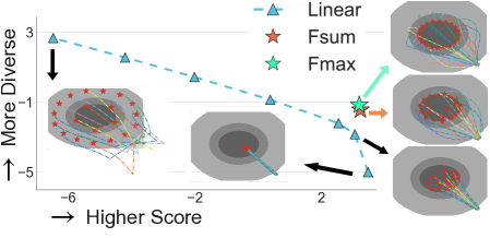
Figure 2: The loss $F$ vs. diversity score $\Phi$ by $F_{\textrm{sum}}$ and $F_{\textrm{max}}$ on a 2D example (the orange and green star), and by minimizing $(1-\alpha)F_{\textrm{sum}}+\alpha\Phi$ with different values of $\alpha\in[0,1]$ (blue triangles). We can see that $F_{\textrm{sum}}$ achieves a better trade-off.

Q2: How does our method compare with the linear combination method? Varying $\alpha$ in the linear combination (e.g. 0, $10^{-4}$, $10^{-3}$, 0.01, 0.1, 0.5, 1), we can trace a (locally optimal) Pareto front of loss $F$ and diversity $\Phi$. In Figure 2, we find that our method can achieve strictly better results than the Pareto front of the linear combination method. Compared to the linear combination (the blue triangles), we notice that in the early iterations of the trajectory, $F_{\textrm{sum}}$ and $F_{\textrm{max}}$ introduce a larger diversity penalty and makes the particles more diverse.

(a)
(b)
(c)
	$F_{\textrm{max}}$		$F_{\textrm{sum}}$

Figure 3: Results on toy examples with $F_{\textrm{max}}$ and $F_{\textrm{sum}}$. The red and orange stars show the 1000th-iteration and 200th-iteration results. The curve shows the value of the target function and diversity term during optimization.

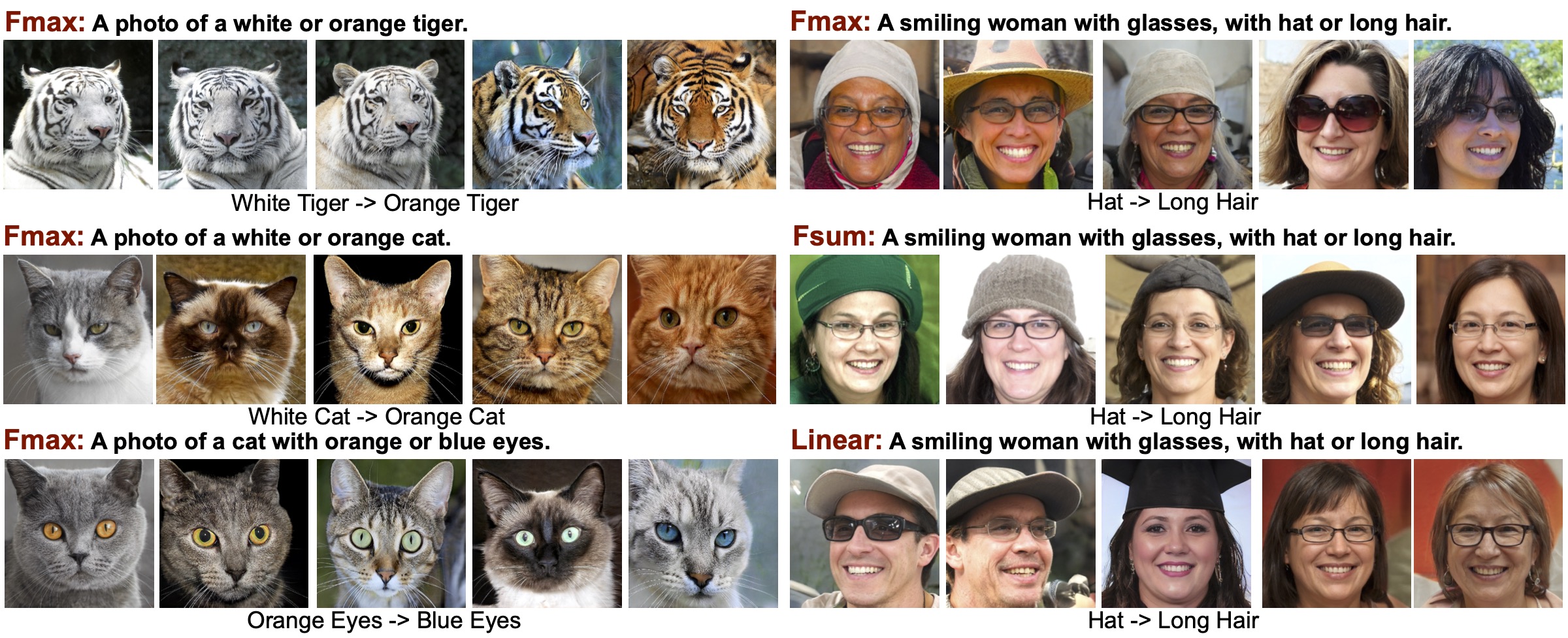
Figure 4: The left column: images generated by $F_{\textrm{max}}$ based on different input text. Right column: images generated by $F_{\textrm{max}}$, $F_{\textrm{sum}}$ and the linear combination (7) ($\alpha=0.5$) from the same input text. The text above each image denotes the text prompt $\mathcal{T}$, and the text under each image displays the $\mathcal{T}_{1}\rightarrow\mathcal{T}_{2}$ used to define the diversity score in (9). Better viewed when zoomed in; see Appendix for more examples.

Q3: What is difference of using $F_{\textrm{max}}$ vs. $F_{\textrm{sum}}$?

As suggested in Section 2, $F_{\textrm{max}}$ is expected to generate more diverse examples, with the trade-off of yielding slower convergence and potentially worse loss value. To verify this, we test $F_{\textrm{max}}$ and $F_{\textrm{sum}}$ in three different kinds of test functions shown in Figure 3, whose optimal set is a connected manifold (Figure 3(a)), multiple isolated modes (Figure 3(b)), and a curve (Figure 3(c)). We observe that: 1) Compared to $F_{\textrm{sum}}$, $F_{\textrm{max}}$ tends to place a larger diversity penalty, especially in the early phase of the optimization. 2) In $F_{\textrm{max}}$, the particles tend to lie on the contour lines during the optimization (Figure 3(a) left).

4.2 Latent Space Exploration for Image Generation

Text-Controlled Zero-shot Image Generation

We apply our method to text-controlled image generation. We base our method on FuseDream (Liu et al., 2021), a training-free text-to-image generator that works by combining the power of pre-trained BigGAN (Brock et al., 2019) and the CLIP model (Radford et al., 2021).

Basic Setup A pre-trained GAN model $\mathcal{I}=g(x)$ is a neural network that takes a latent vector $x\in\mathbb{R}^{d}$ and outputs an image $\mathcal{I}$. The CLIP model (Radford et al., 2021) provides a score $\texttt{CLIP}(\mathcal{T},\mathcal{I})$ for how an image $\mathcal{I}$ is related to a text prompt $\mathcal{T}$. We use the augmented clip score $s_{\texttt{AugCLIP}}(\mathcal{T},\mathcal{I})$ from Liu et al. (2021) which improves the robustness by introducing random augmentation on images.

Liu et al. (2021) generates an image $\mathcal{I}=g(x)$ for a given text $\mathcal{T}$ by solving $\max_{x}s_{\texttt{AugCLIP}}(\mathcal{T},g(x))$. We introduce diversity on top of Liu et al. (2021). Given text prompt $\mathcal{T}$, our goal is to find a diversified set of images $\mathcal{I}=g(x_{i})$, $\forall i\in[m]$ that maximize the $s_{\texttt{AugCLIP}}$ score, where $\boldsymbol{x}=\{x_{1},\ldots,x_{m}\}$ is obtained by

$$\min_{\boldsymbol{x}}\Phi(\boldsymbol{x}),~{}~{}s.t.~{}~{}\boldsymbol{x}\subseteq\arg\max_{\boldsymbol{x}^{\prime}}s_{\texttt{AugCLIP}}(\mathcal{T},g(\boldsymbol{x}^{\prime})),$$ (8)

where we define the diversity score by $\Phi(\boldsymbol{x})=\Phi_{s}(\psi(x_{1}),\ldots,\psi(x_{m}))$, and $\psi$ is a neural network that an input image to a semantic space. In particular, we use

$$\psi(x)=\bigg{[}s_{\texttt{AugCLIP}}\left(\mathcal{T}_{1},g(x)\right),s_{\texttt{AugCLIP}}\left(\mathcal{T}_{2},g(x)\right)\bigg{]},$$ (9)

where $\mathcal{T}_{1}$ and $\mathcal{T}_{2}$ are two text that specify the semantic directions along which we want to diversify. For example, by taking $\mathcal{T}_{1}$ = ‘White Tiger’ and $\mathcal{T}_{2}$ = ‘Orange Tiger’ (Figure 4), we can find images of tigers that interprets from white to orange.

For the experiments, we use the Adam (Kingma & Ba, 2014) optimizer with constant $5\times 10^{-3}$ learning rate. For BigGAN, the optimizable variable $x$ contains two parts, a feature vector in the GAN latent space and a class vector representing the 1K ImageNet classes. We set the number of iterations to 500 following Liu et al. (2021). For StyleGAN-v2 (Karras et al., 2020), the optimizable variable $x$ is a feature vector in the GAN latent space. Because StyleGAN-v2 generates images in higher resolution (e.g. 1024$\times$1024), we set the number of iterations to 50 to save computation cost.

Qualitative Analysis

Figure 4 shows examples of images generated from our $F_{\textrm{max}}$, $F_{\textrm{sum}}$ and the linear combination ($\alpha=0.5$) when using StyleGAN-v2 trained on FFHQ (Karras et al., 2019) and AFHQ (Choi et al., 2020). We can see that the images generated by ours are both high quality, semantically related to the prompt $\mathcal{T}$ (high $s_{\texttt{AugCLIP}}$), and well-diversified along semantic direction specified by $\mathcal{T}_{1}$ and $\mathcal{T}_{2}$ (low $\Phi(\boldsymbol{x})$). For example, for $\mathcal{T}$=‘a smiling woman with glasses’, $\mathcal{T}_{1}$=’hat’, $\mathcal{T}_{2}$=’long hair’, our method yields images with diverse hats and hair lengths. As a comparison, the $\alpha=0.5$ linear combination fails to generate ‘woman’ or ‘glasses’ in some cases.

	$\mathcal{T}$	$\mathcal{T}_{1}$	$\mathcal{T}_{2}$	Linear $\alpha=0$		Linear $\alpha=0.5$		$F_{\textrm{sum}}$		$F_{\textrm{max}}$
				Sc $\uparrow$	Div $\uparrow$	Sc $\uparrow$	Div $\uparrow$	Sc $\uparrow$	Div $\uparrow$	Sc $\uparrow$	Div $\uparrow$
Test 1	A painting of an either blue or red dog.	blue	red	0.34	-3.78	0.30	-3.63	0.34	-3.64	0.31	-3.60
Test 2	A campus with river or forest.	forest and trees	river	0.27	-3.81	0.25	-3.72	0.28	-3.72	0.26	-3.68
Test 3	Red, Blue and Yellow Squares	Mondrian	Vincent van Gogh	0.31	-3.80	0.26	-3.71	0.30	-3.71	0.26	-3.66
Test 4	Home-cooked meal in Russia.	sausage, meat	tomato, onion	0.29	-3.80	0.27	-3.64	0.29	-3.65	0.27	-3.61

Table 1: The diversity score (Div) and the AugCLIP score (Sc) our different methods on text-to-image generation.

$s_{\texttt{AugCLIP}}$	Diversity
Iterations	$s_{\texttt{AugCLIP}}$	$s_{\texttt{AugCLIP}}$	$s_{\texttt{AugCLIP}}$	$s_{\texttt{AugCLIP}}$
(a) Test 1	(b) Test 1	(c) Test 2	(d) Test 3	(e) Test 4

Figure 5: (a) The AugCLIP score vs. iteration in Test 1 in Table 1. (b)-(d) The (quality, diversity) front of $F_{\textrm{sum}}$ (blue), $F_{\textrm{max}}$ (yellow), linear combination with $\alpha\in\{0,0.25,0.5,0.75\}$ (red), and ‘finetuned’ linear combination with the same set of $\alpha$ (Cyan). Here ‘finetune’ refers to optimizing the linearly combined loss in (7) for 250 iterations and then optimize $s_{\texttt{AugCLIP}}(\cdot)$ for another 250 iterations with the diversity term turned off. $F_{\textrm{sum}}$ and $F_{\textrm{max}}$ outperform both variants of linear combination.

Quantitative Analysis We present the value of quality score $s_{\texttt{AugCLIP}}$ and diversity score $\Phi$ given by our methods ($F_{\textrm{max}}$ and $F_{\textrm{sum}}$) and the linear combination method (7) on an additional set of examples. In Table 1 and Figure 5, we can see that that $F_{\textrm{max}}$ and $F_{\textrm{sum}}$ always achieve better results than tuning the coefficient value for the linear combination. $F_{\textrm{max}}$ generates more diverse results while $F_{\textrm{sum}}$ optimizes the main loss better. We also find that if we finetune the linear combination result by turning off the diversity promoting loss at the end of the optimization, it does not improve the (quality, diversity) Pareto front (see Figure 5). Figure 6 shows more detailed analysis on the Test 1.

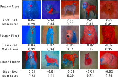
Figure 6: Images for Test 1 in Table 1. ‘Linear’ refers to the linear combination ($\alpha=0.5$). There are two numbers under each image: the numbers on the top row are $s_{\texttt{AugCLIP}}\left(\mathcal{T}_{1},g(x_{i})\right)-s_{\texttt{AugCLIP}}\left(\mathcal{T}_{2},g(x_{i})\right)$, which reflects the percentage of blue vs. red colors; the numbers on the second row are $s_{\texttt{AugCLIP}}$. See Appendix for more examples.

Test	MEGA			$F_{\textrm{sum}}$
	Sc $\uparrow$	Div $\uparrow$	Hours $\downarrow$	Sc $\uparrow$	Div $\uparrow$	Hours $\downarrow$
1	0.35	-3.62	0.97	0.34	-3.64	0.16
2	0.28	-3.71		0.28	-3.72
3	0.32	-3.69		0.30	-3.71
4	0.29	-3.66		0.29	-3.65

Table 2: Comparison with MEGA. Hours is measured on a NVIDIA GeForce RTX3090 GPU.

Test	Iteration: 250				Iteration: 500
	Gong et al. (2021)		$F_{\textrm{sum}}$		Gong et al. (2021)		$F_{\textrm{sum}}$
	Sc $\uparrow$	Div $\uparrow$	Sc $\uparrow$	Div $\uparrow$	Sc $\uparrow$	Div $\uparrow$	Sc $\uparrow$	Div $\uparrow$
1	0.26	-3.62	0.31	-3.66	0.32	-3.65	0.34	-3.64
2	0.23	-3.68	0.26	-3.73	0.26	-3.71	0.28	-3.72
3	0.24	-3.67	0.28	-3.71	0.27	-3.71	0.30	-3.71
4	0.23	-3.62	0.26	-3.64	0.27	-3.63	0.29	-3.65

Table 3: Comparison with Gong et al. (2021).

Compare with MEGA We compare with MAP-Elites via a Gradient Arborescence (MEGA) (Fontaine & Nikolaidis, 2021), a recent improvement of MAP-Elites (Mouret & Clune, 2015) in Table 2. Compared with MEGA, we find that our method requires far less optimization time (1 hours v.s. 10 minutes) and achieves comparable results. See Appendix for more detailed comparisons.

Compare with Gong et al. (2021) Gong et al. (2021) provides an off-the-shelf method for solving general lexicographic optimization of form (3). We apply it to the case of $F=F_{\textrm{sum}}$ and compare it with our $F_{\textrm{sum}}$ method in Table 3. Our $F_{\textrm{sum}}$ method yields faster convergence on the main loss, and Gong et al. (2021) also outperforms the linear combination baseline with $\alpha=0.5$ shown in Table 1. On the other hand, we find that Gong et al. (2021) fails to work when $F=F_{\textrm{max}}$ due to the non-smoothness of the max function.

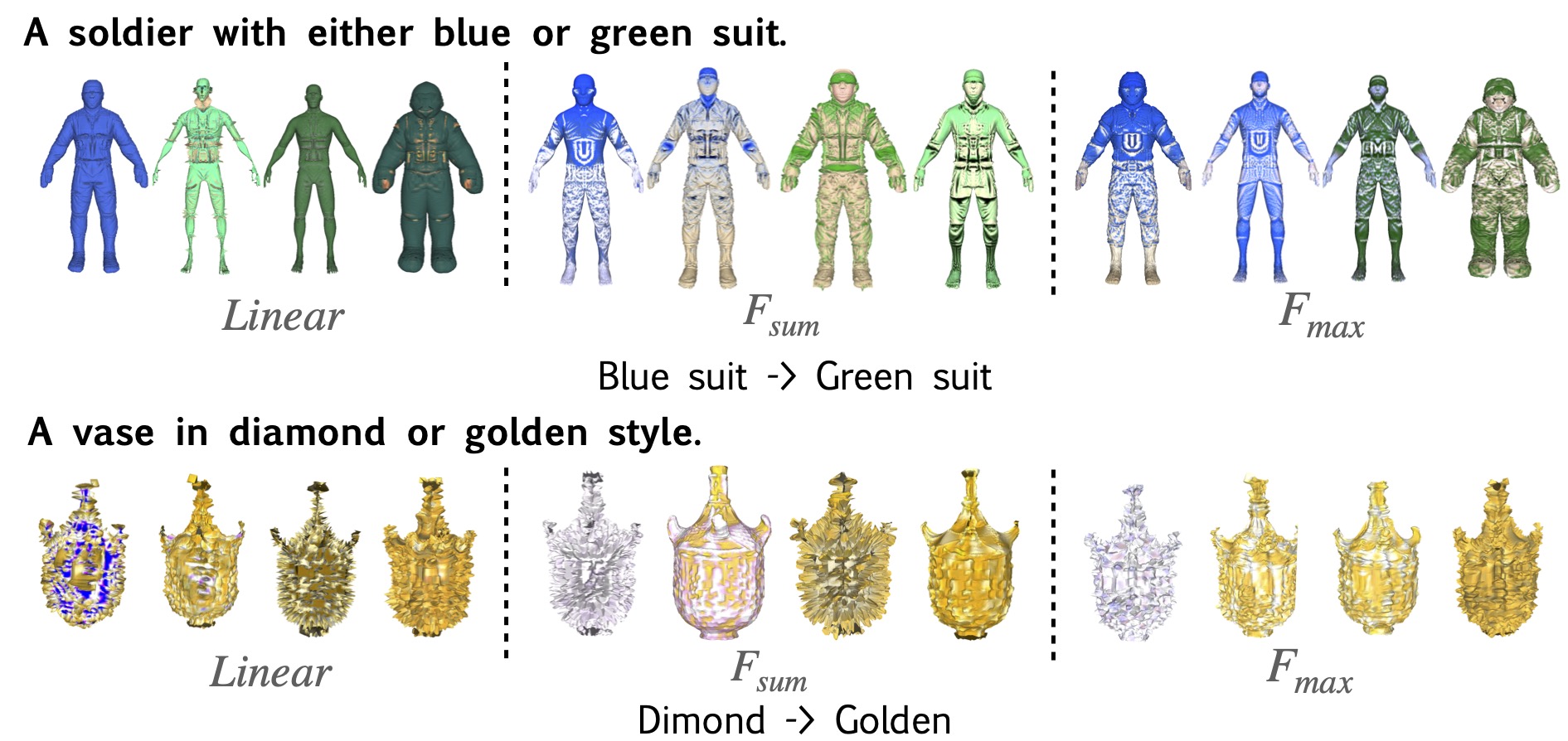
Figure 7: Results on Text2Mesh generation form $F_{\textrm{sum}}$, $F_{\textrm{max}}$ and linear combination ($\alpha=0.5$). See supplementary materials for a detailed description video.

4.3 Controllable Diverse Generation on Meshes

We apply our method to generate diversified meshes of 3D objectives from text. We base our method on Text2Mesh (Michel et al., 2021), and promote the diversity with a CLIP-based semantic diversity score similar to (9) that is based on a pair of test $\mathcal{T}_{1},\mathcal{T}_{2}$. See Appendix for more detailed setup.

Figure 7 shows the result of the $F_{\textrm{sum}}$, $F_{\textrm{max}}$ and the linear combination method $\alpha=0.5$. We set $\alpha=0.5$ to have a similar diversity score with the $F_{\textrm{sum}}$, $F_{\textrm{max}}$ methods. We run 1,500 iterations for $F_{\textrm{sum}}$ and $F_{\textrm{max}}$. For the linear combination method, we apply the diversity term for 750 steps and finetune for another 750 steps with the diversity promotion turned off. We can see that $F_{\textrm{sum}}$ and $F_{\textrm{max}}$ generate the 3D models with different cloth styles in the green and blue colors which satisfy the text prompt. On contrast, the linear combination baseline fails to keep the reasonable geometry and provide a reasonable color; see e.g., the overly-thin and overly-thick mesh displacement on soldier case, and the non-smoothing meshes and the purple color in vase case.

4.4 Diversified Molecular Conformation Generation

A fundamental problem in computational chemistry is molecular conformation generation, predicting stable 3D structures from 2D molecular graphs. The goal is to take a 2D molecular graph representation $G$ of a molecule and predict its 3D conformation (i.e., the 3D coordinates of the atoms in the molecule). Diversity is essential in this problem since there are multiple possible conformations of a single molecule and we hope to predict all of them.

Specifically, we are interested in generating a set of possible conformations $\boldsymbol{x}=\{x_{1},\ldots x_{m}\}$ of a given molecule, where $x_{i}\in\mathbb{R}^{3\times d}$ is the 3D coordinates of $d$ atoms in the molecule. Let $E(x)$ be an energy function of which the true configurations are local minima, we generate $\boldsymbol{x}$ by solving

$$\min_{\boldsymbol{x}}\Phi_{s}(\boldsymbol{x}),~{}~{}s.t.~{}~{}\boldsymbol{x}\subseteq\arg\min E.$$ (10)

For our experiments, we adopt the energy function from ConfGF (Shi et al., 2021), which is implicitly defined with a learnable gradient field trained on the GEOM-QM9 dataset (Axelrod & Gomez-Bombarelli, 2020).

We evaluate the method by comparing the conformations predicted from (10) with the set of ground truth conformations (denoted by $\boldsymbol{x}^{*}$) of the molecule of interest from GEOM-QM9. Because the 3D coordinates are unique upto rotation and translation. We measure the difference between two conformations $x,x^{\prime}$ using the root mean square deviation: $\text{RMSD}(x,x^{\prime})=\min_{T}\left\lVert T(x)-x^{\prime}\right\rVert_{2}$, where $T$ is minimized on the set of all possible rotations and translations. For the set of predicted $\boldsymbol{x}$ and ground truth $\boldsymbol{x}^{*}$ conformations, we calculate the matching score (MAT) for evaluating quality and the coverage score (COV) to measure diversity following Shi et al. (2021),

$$\text{COV}(\boldsymbol{x},\boldsymbol{x}^{*})={\sharp\{x^{*}\in\boldsymbol{x}^{*}|\text{RMSD}(x^{*},x)<\delta,x\in\boldsymbol{x}\}}/\sharp\boldsymbol{x}^{*},$$

$$\text{MAT}(\boldsymbol{x},\boldsymbol{x}^{*})=\sum_{x\in\boldsymbol{x}^{*}}\min_{x\in\boldsymbol{x}}\text{RMSD}(x^{*},x)/\sharp\boldsymbol{x}^{*},$$

where $\sharp$ denotes the number of elements of a set. Both COV and MAT measure the precision of the prediction (how may predictions are found in ground truth list); to measure recall (how every ground truth conformation is found by at least a prediction), we also calculate $\text{RMAT}(\boldsymbol{x},\boldsymbol{x}^{*}):=\text{MAT}(\boldsymbol{x}^{*},\boldsymbol{x})$, the recall matching score (RMAT).

Baselines We use the same model trained from ConfGF and use our $F_{\textrm{sum}}$ and $F_{\textrm{max}}$ method as a way to enhance diversification during inference. We test two inference strategies for both our method and the baselines: One is the original ConfGF strategy, which randomly initializes $2\times\sharp\boldsymbol{x}^{*}$ number of conformations and filters half of them to get $1\times\sharp\boldsymbol{x}^{*}$ number of predicted conformations. The original inference strategy of ConfGF can be viewed as a naive multi-initialization strategy. We also test another strategy that directly predicts $\sharp\boldsymbol{x}^{*}$ confirmations as $\boldsymbol{x}^{*}$. We denote these two baselines as $2\times$Ref and $1\times$Ref, respectively.

# Init	Method	COV (%) $\uparrow$		MAT ($\mathring{\text{A}}$) $\downarrow$		RMAT ($\mathring{\text{A}}$) $\downarrow$
	ConfGF	77.7	78.0	0.338	0.346	0.530	0.514
$1\times$Ref	$F_{\textrm{sum}}$	79.2	80.9	0.332	0.339	0.504	0.490
	$F_{\textrm{max}}$	79.4	80.5	0.336	0.340	0.512	0.501
	ConfGF	90.0	94.6	0.267	0.269	0.502	0.499
$2\times$Ref	$F_{\textrm{sum}}$	90.3	94.9	0.270	0.268	0.483	0.475
	$F_{\textrm{max}}$	89.8	94.3	0.273	0.271	0.495	0.497

Table 4: Results on diversified molecule conformation generation using $F_{\textrm{sum}}$, $F_{\textrm{max}}$ and the linear combination method.

Results See the results in Table 4. We find that both $F_{\textrm{sum}}$ and $F_{\textrm{max}}$ yield better results than the baseline in all the metrics (e.g. COV, MAT, and RMAT), and $F_{\textrm{sum}}$ yields the best COV diversity score and Pareto front (precision, recall) among all methods.

4.5 Training Ensemble Neural Networks

Another natural application of our method is learning diversified neural network ensembles. Let $\theta$ be the parameter of a neural network model. We are interested in learning a set of neural networks $\boldsymbol{\theta}=(\theta_{1},\ldots,\theta_{m})$ by solving

$$\vspace{-5pt}\min_{\boldsymbol{\theta}}\Phi(\boldsymbol{\theta}),~{}~{}s.t.~{}~{}\boldsymbol{\theta}\subseteq\arg\min\ell_{\text{train}},\vspace{-5pt}$$ (11)

where $\ell_{\text{train}}(\theta)$ is a standard training loss of the neural network, and $\Phi(\boldsymbol{\theta})=\mathbb{E}_{x\sim\mathcal{D}}[\Phi_{s}(f_{\theta_{1}}(x)\ldots f_{\theta_{m}}(x))]$ is the diversity defined w.r.t. the hidden nodes of the last layer $f_{\theta}$ of the neural networks on training data $\mathcal{D}$.

	Linear Combination			$F_{\textrm{sum}}$	$F_{\textrm{max}}$
	$0.0$	$0.1$	$0.9$
Single Acc $\uparrow$	91.4	90.9	89.8	91.2	90.7
Ensemble Acc $\uparrow$	92.0	91.4	90.5	92.0	91.3
Diversity $\uparrow$	-4.11	-4.04	-4.01	-4.07	-4.03
ECE $\downarrow$	4.03	3.39	3.53	3.38	3.51

Table 5: Results on learning diversified ensemble neural networks with $F_{\textrm{sum}}$, $F_{\textrm{max}}$ and the linear combination with $\alpha\in\{0,0.1,0.9\}.$

Results Table 5 shows the results when we train three $(m=3)$ ResNet-56 models on CIFAR-10 dataset. We observe that the linear combination often hurts the single network accuracy and hence yields poorer accuracy compared to the case without diversity regularization ($\alpha=0$). In comparison, $F_{\textrm{sum}}$ improves both the diversity and ECE score without hurting the model accuracy and achieves the best accuracy-diversity trade-off.

5 Conclusion

In this work, we propose a framework of gradient-based optimization methods to find diverse points in the optimum set of a loss function with a harmless diversity promotion mechanism. We find that our methods yield both diverse and high-quality solutions on a broad spectrum of applications. Another important application that we have not explored is robotics, finding diverse policies of critically important for planning and reinforcement learning. We will explore it in future works.

Appendix A Details about Generation on Meshes

Let $\mathcal{M}=g(\boldsymbol{x})$ be a mesh generator, and $I=P(\mathcal{M})$ be a differentiable render that generates (a set of) images from the three objective specified by $\mathcal{M}$. Given a text prompt $\mathcal{T}$, and a diversity score $\Phi$, we want to find a diverse set of meshes $\mathcal{M}_{i}=g(x_{i})$ by solving

$$\min_{\boldsymbol{x}}\Phi(\boldsymbol{x})~{}~{}~{}s.t.~{}~{}~{}\boldsymbol{x}\in\arg\min_{\boldsymbol{x}^{\prime}}s_{\texttt{CLIP}}(\mathcal{T},P(g(\boldsymbol{x}^{\prime}))),$$

where $\Phi(\boldsymbol{x})=\Psi_{s}(\psi(\boldsymbol{x}))$ with $\psi$ defined similar to (9) based on a pair of text $\mathcal{T}_{1}$, $\mathcal{T}_{2}$:

$$\psi(x)=\bigg{[}s_{\texttt{CLIP}}(\mathcal{T}_{1},P(g(x))),s_{\texttt{CLIP}}(\mathcal{T}_{2},P(g(x)))\bigg{]}.$$

We follow the model architecture and generation pipeline in Text2Mesh (Michel et al., 2021). Text2Mesh proposes a neural style field network, which directly outputs the value displacement on the mesh normal and the color on each vertex. A differentiable renderer is then rendering multiple 2D views for the styled mesh as the image set. The pipeline wants to get a higher CLIP-based similarity score between the rendered image set and query text. Similar to image generation, we create the diversity measure with additional text prompts and hope to make the Text2mesh model generate a variety of different mesh styles with RGB colors and textures. We apply four same meshes with the zero RGB color and geometry displacement and then optimize the color and displacement variables with 1,500 steps. We attach videos for the results in Figure 7 in the supplementary material for a better visualization with more angles.

Appendix B More Examples

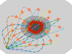
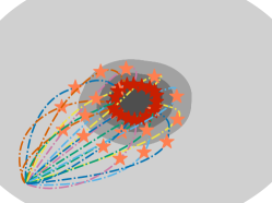
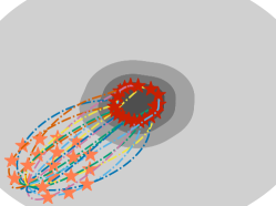
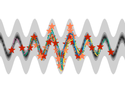
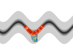
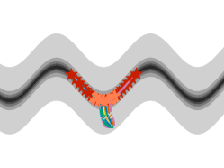
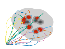
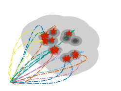
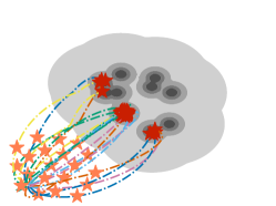
$F_{\textrm{max}}$	$F_{\textrm{sum}}$	Gong et al. (2021)

Figure 8: Results on toy examples with $F_{\textrm{max}}$, $F_{\textrm{sum}}$ and Gong et al. (2021) . We notice that $F_{\textrm{max}}$ and $F_{\textrm{sum}}$ empirically converge faster. For multi-modal examples, our version captures more modals than Gong et al. (2021).

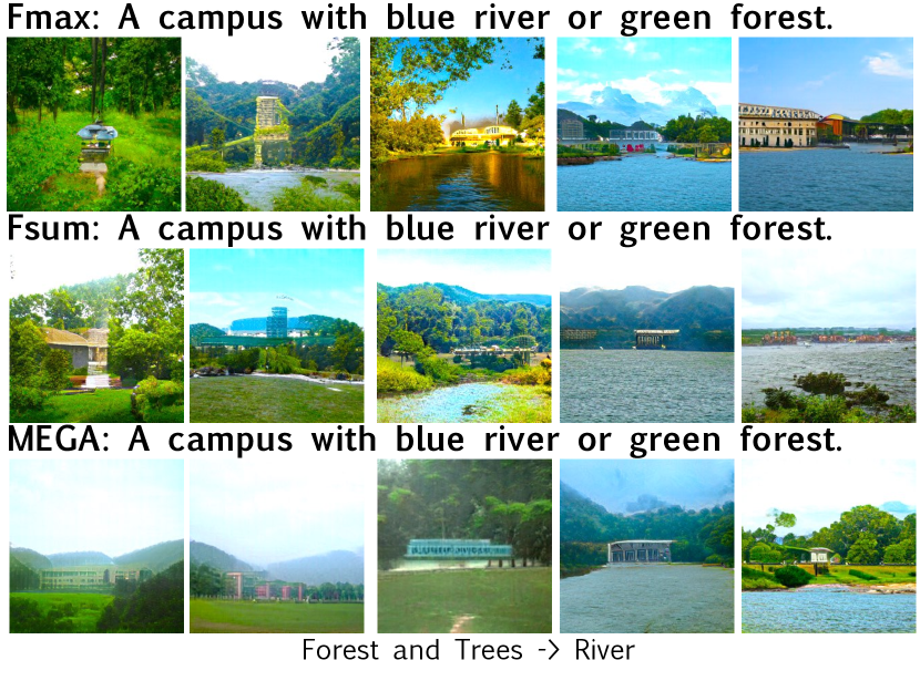
Figure 9: Results on the test function 2 in Table 1. We notice $F_{\textrm{max}}$, $F_{\textrm{sum}}$ and MEGA achieve comparable quality and diversity, while $F_{\textrm{max}}$ and $F_{\textrm{sum}}$ uses less time as shown in Table 2.

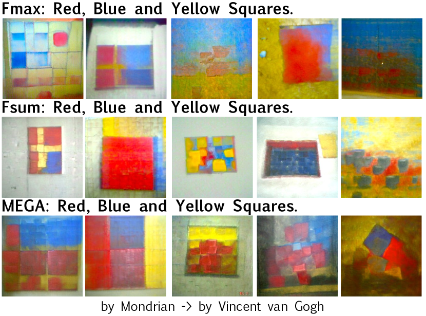
Figure 10: Results on the test function 3 in Table 1. We notice $F_{\textrm{max}}$, $F_{\textrm{sum}}$ and MEGA achieve comparable quality and diversity, while $F_{\textrm{max}}$ and $F_{\textrm{sum}}$ uses less time as shown in Table 2.

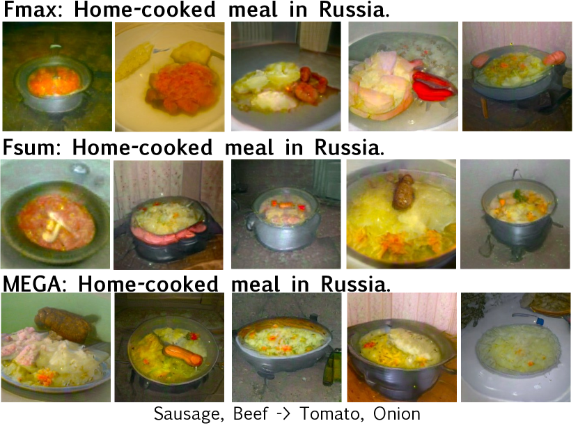
Figure 11: Results on the test function 4 in Table 1. We notice $F_{\textrm{max}}$, $F_{\textrm{sum}}$ and MEGA achieve comparable quality and diversity, while $F_{\textrm{max}}$ and $F_{\textrm{sum}}$ uses less time as shown in Table 2.

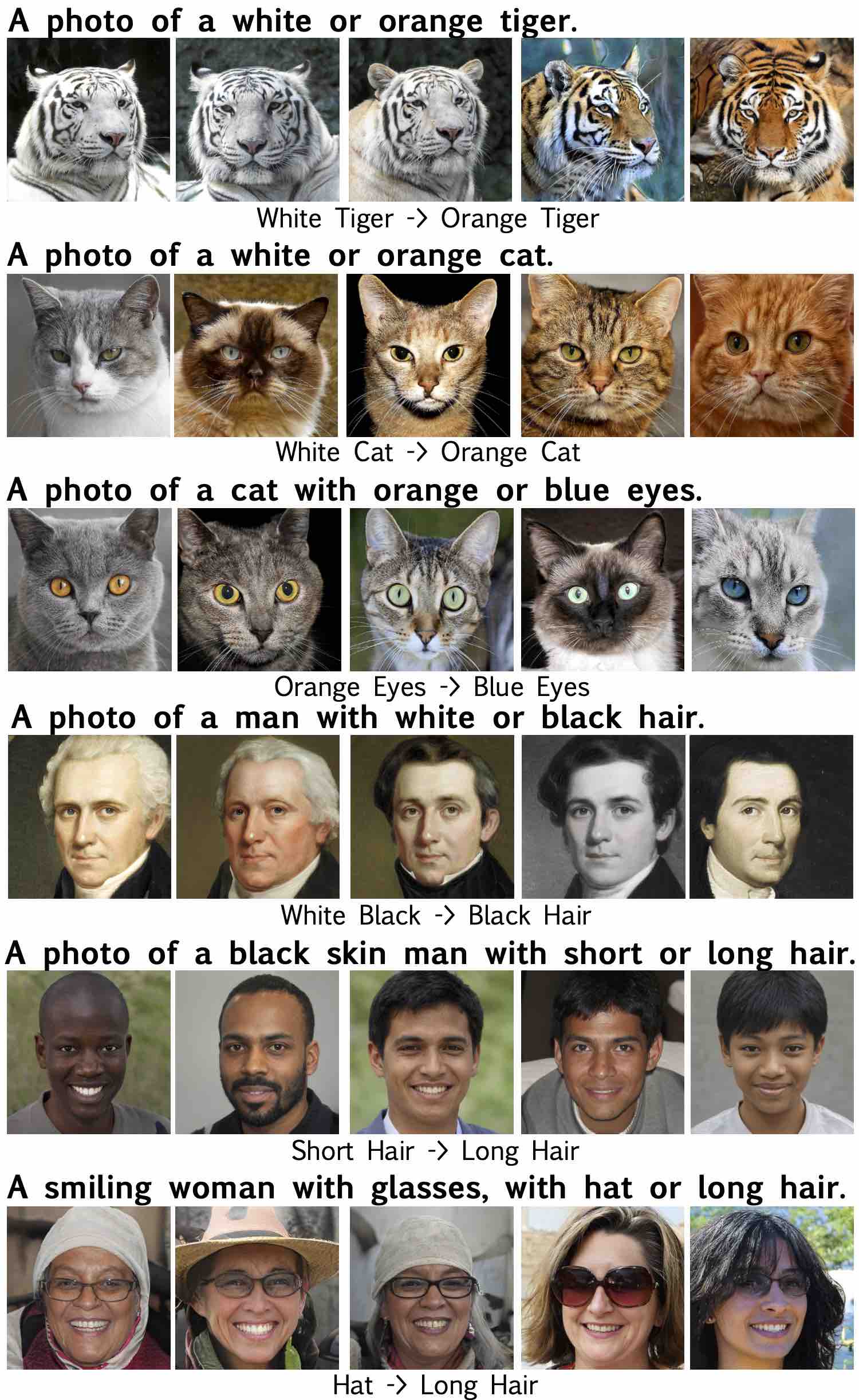
Figure 12: We apply $F_{\textrm{max}}$ to pre-trained StyleGAN-v2 checkpoints. The text above each image denotes $\mathcal{T}$, while the text under each image displays $\mathcal{T}_{1}\rightarrow\mathcal{T}_{2}$.

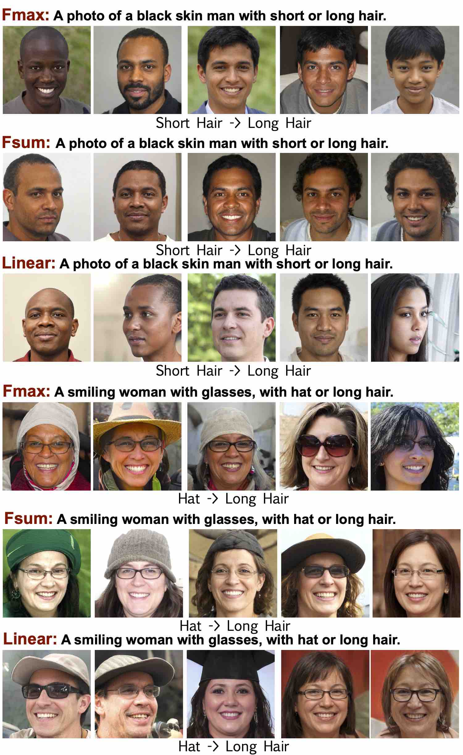
Figure 13: We apply $F_{\textrm{max}}$, $F_{\textrm{sum}}$ and the linear combination (7) ($\alpha=0.5$) to StyleGAN-v2 pre-trained on FFHQ (Karras et al., 2019). The text above each image denotes $\mathcal{T}$, while the text under each image displays $\mathcal{T}_{1}\rightarrow\mathcal{T}_{2}$.

We display more examples of different methods in this section.

In Figure 8, we compare our method with Lexico (Gong et al., 2021). We notice that by 1) replacing the inner product constraint with quadratic constraint, 2) changing $F$ function, our approaches yield faster convergence than Lexico, and capture more local modal for the multiple modal objective.

In Figure 9, 10 and 11, we list the optimization results for $F_{\textrm{max}}$, $F_{\textrm{sum}}$ and MEGA, the evolutionary algorithm. Visually, these methods achieve similar performance, while our approaches spend less time as shown in Section 4.

In Figure 12, we demonstrate the results of $F_{\textrm{max}}$ and $F_{\textrm{sum}}$, and both achieve good performance. We use the checkpoints provided by StyleGAN-v2 . For cats and tigers, we use the checkpoint trained on AFHQ Cat and AFHQ Wild using adaptive discriminator augmentation.. For people face, we use the checkpoint trained on FFHQ at 1024$\times$1024 resolution. For portraitures, we use the checkpoint trained on MetFaces at 1024$\times$1024 resolution, which does transfers learning from FFHQ using adaptive discriminator augmentation.

References

- Axelrod & Gomez-Bombarelli (2020) Axelrod, S. and Gomez-Bombarelli, R. Geom: Energy-annotated molecular conformations for property prediction and molecular generation. arXiv preprint arXiv:2006.05531, 2020.
- Brock et al. (2019) Brock, A., Donahue, J., and Simonyan, K. Large scale GAN training for high fidelity natural image synthesis. In International Conference on Learning Representations, 2019. URL https://openreview.net/forum?id=B1xsqj09Fm.
- Brown et al. (2020) Brown, T. B., Mann, B., Ryder, N., Subbiah, M., Kaplan, J., Dhariwal, P., Neelakantan, A., Shyam, P., Sastry, G., Askell, A., et al. Language models are few-shot learners. arXiv preprint arXiv:2005.14165, 2020.
- Choi et al. (2020) Choi, Y., Uh, Y., Yoo, J., and Ha, J.-W. Stargan v2: Diverse image synthesis for multiple domains. In Proceedings of the IEEE/CVF Conference on Computer Vision and Pattern Recognition, pp. 8188–8197, 2020.
- Conti et al. (2017) Conti, E., Madhavan, V., Such, F. P., Lehman, J., Stanley, K. O., and Clune, J. Improving exploration in evolution strategies for deep reinforcement learning via a population of novelty-seeking agents. arXiv preprint arXiv:1712.06560, 2017.
- Croce & Hein (2020) Croce, F. and Hein, M. Reliable evaluation of adversarial robustness with an ensemble of diverse parameter-free attacks. In International conference on machine learning, pp. 2206–2216. PMLR, 2020.
- Cully et al. (2015) Cully, A., Clune, J., Tarapore, D., and Mouret, J.-B. Robots that can adapt like animals. Nature, 521:503–507, 2015.
- De Boer et al. (2005) De Boer, P.-T., Kroese, D. P., Mannor, S., and Rubinstein, R. Y. A tutorial on the cross-entropy method. Annals of operations research, 134(1):19–67, 2005.
- Fedus et al. (2021) Fedus, W., Zoph, B., and Shazeer, N. Switch transformers: Scaling to trillion parameter models with simple and efficient sparsity. arXiv preprint arXiv:2101.03961, 2021.
- Flageat & Cully (2020) Flageat, M. and Cully, A. Fast and stable map-elites in noisy domains using deep grids. In Artificial Life Conference Proceedings, pp. 273–282. MIT Press, 2020.
- Fontaine & Nikolaidis (2021) Fontaine, M. C. and Nikolaidis, S. Differentiable quality diversity. arXiv e-prints, pp. arXiv–2106, 2021.
- Gomes et al. (2013) Gomes, J., Urbano, P., and Christensen, A. L. Evolution of swarm robotics systems with novelty search. Swarm Intelligence, 7(2):115–144, 2013.
- Gong et al. (2021) Gong, C., Liu, X., and Liu, Q. Automatic and harmless regularization with constrained and lexicographic optimization: A dynamic barrier approach. Advances in Neural Information Processing Systems, 34, 2021.
- Götz (2003) Götz, M. On the riesz energy of measures. Journal of Approximation Theory, 122(1):62–78, 2003.
- Gravina et al. (2018) Gravina, D., Liapis, A., and Yannakakis, G. N. Quality diversity through surprise. IEEE Transactions on Evolutionary Computation, 23(4):603–616, 2018.
- Hansen et al. (2003) Hansen, N., Müller, S. D., and Koumoutsakos, P. Reducing the time complexity of the derandomized evolution strategy with covariance matrix adaptation (cma-es). Evolutionary computation, 11(1):1–18, 2003.
- Karras et al. (2019) Karras, T., Laine, S., and Aila, T. A style-based generator architecture for generative adversarial networks. In Proceedings of the IEEE/CVF Conference on Computer Vision and Pattern Recognition, pp. 4401–4410, 2019.
- Karras et al. (2020) Karras, T., Laine, S., Aittala, M., Hellsten, J., Lehtinen, J., and Aila, T. Analyzing and improving the image quality of StyleGAN. In Proc. CVPR, 2020.
- Kingma & Ba (2014) Kingma, D. P. and Ba, J. Adam: A method for stochastic optimization. arXiv preprint arXiv:1412.6980, 2014.
- Kuijlaars et al. (2007) Kuijlaars, A., Saff, E., and Sun, X. On separation of minimal riesz energy points on spheres in euclidean spaces. Journal of computational and applied mathematics, 199(1):172–180, 2007.
- Lakshminarayanan et al. (2016) Lakshminarayanan, B., Pritzel, A., and Blundell, C. Simple and scalable predictive uncertainty estimation using deep ensembles. arXiv preprint arXiv:1612.01474, 2016.
- Lee et al. (2018) Lee, H.-Y., Tseng, H.-Y., Huang, J.-B., Singh, M., and Yang, M.-H. Diverse image-to-image translation via disentangled representations. In Proceedings of the European conference on computer vision (ECCV), pp. 35–51, 2018.
- Lehman & Stanley (2011a) Lehman, J. and Stanley, K. O. Abandoning objectives: Evolution through the search for novelty alone. Evolutionary computation, 19(2):189–223, 2011a.
- Lehman & Stanley (2011b) Lehman, J. and Stanley, K. O. Evolving a diversity of virtual creatures through novelty search and local competition. In Proceedings of the 13th annual conference on Genetic and evolutionary computation, pp. 211–218, 2011b.
- Liu & Wang (2016) Liu, Q. and Wang, D. Stein variational gradient descent: A general purpose bayesian inference algorithm. arXiv preprint arXiv:1608.04471, 2016.
- Liu et al. (2021) Liu, X., Gong, C., Wu, L., Zhang, S., Su, H., and Liu, Q. Fusedream: Training-free text-to-image generation with improved clip+gan space optimization, 2021.
- Michel et al. (2021) Michel, O., Bar-On, R., Liu, R., Benaim, S., and Hanocka, R. Text2mesh: Text-driven neural stylization for meshes. arXiv preprint arXiv:2112.03221, 2021.
- Mouret & Clune (2015) Mouret, J.-B. and Clune, J. Illuminating search spaces by mapping elites. arXiv preprint arXiv:1504.04909, 2015.
- Osa (2020) Osa, T. Multimodal trajectory optimization for motion planning. The International Journal of Robotics Research, 39(8):983–1001, 2020.
- Pang et al. (2019) Pang, T., Xu, K., Du, C., Chen, N., and Zhu, J. Improving adversarial robustness via promoting ensemble diversity. In International Conference on Machine Learning, pp. 4970–4979. PMLR, 2019.
- Parker-Holder et al. (2020) Parker-Holder, J., Pacchiano, A., Choromanski, K., and Roberts, S. Effective diversity in population based reinforcement learning. arXiv preprint arXiv:2002.00632, 2020.
- Radford et al. (2021) Radford, A., Kim, J. W., Hallacy, C., Ramesh, A., Goh, G., Agarwal, S., Sastry, G., Askell, A., Mishkin, P., Clark, J., et al. Learning transferable visual models from natural language supervision. arXiv preprint arXiv:2103.00020, 2021.
- Ramesh et al. (2021) Ramesh, A., Pavlov, M., Goh, G., Gray, S., Voss, C., Radford, A., Chen, M., and Sutskever, I. Zero-shot text-to-image generation. arXiv preprint arXiv:2102.12092, 2021.
- Sfikas et al. (2021) Sfikas, K., Liapis, A., and Yannakakis, G. N. Monte carlo elites: quality-diversity selection as a multi-armed bandit problem. arXiv preprint arXiv:2104.08781, 2021.
- Shi et al. (2021) Shi, C., Luo, S., Xu, M., and Tang, J. Learning gradient fields for molecular conformation generation. arXiv preprint arXiv:2105.03902, 2021.
- Toscano-Palmerin & Frazier (2018) Toscano-Palmerin, S. and Frazier, P. Effort allocation and statistical inference for 1-dimensional multistart stochastic gradient descent. In 2018 Winter Simulation Conference (WSC), pp. 1850–1861. IEEE, 2018.
- Vannoy & Xiao (2008) Vannoy, J. and Xiao, J. Real-time adaptive motion planning (ramp) of mobile manipulators in dynamic environments with unforeseen changes. IEEE Transactions on Robotics, 24(5):1199–1212, 2008.
- Wu et al. (2017) Wu, J., Poloczek, M., Wilson, A. G., and Frazier, P. I. Bayesian optimization with gradients. arXiv preprint arXiv:1703.04389, 2017.
- Xie et al. (2015) Xie, P., Deng, Y., and Xing, E. Diversifying restricted boltzmann machine for document modeling. In Proceedings of the 21th ACM SIGKDD International Conference on Knowledge Discovery and Data Mining, pp. 1315–1324, 2015.
- Xie et al. (2016) Xie, P., Zhu, J., and Xing, E. Diversity-promoting bayesian learning of latent variable models. In International Conference on Machine Learning, pp. 59–68. PMLR, 2016.