Flat tori with large Laplacian
eigenvalues in dimensions up to eight

Abstract.

We consider the optimization problem of maximizing the $k$-th Laplacian eigenvalue, $\lambda_{k}$, over flat $d$-dimensional tori of fixed volume. For $k=1$, this problem is equivalent to the densest lattice sphere packing problem. For larger $k$, this is equivalent to the NP-hard problem of finding the $d$-dimensional (dual) lattice with longest $k$-th shortest lattice vector. As a result of extensive computations, for $d\leq 8$, we obtain a sequence of flat tori, $T_{k,d}$, each of volume one, such that the $k$-th Laplacian eigenvalue of $T_{k,d}$ is very large; for each (finite) $k$ the $k$-th eigenvalue exceeds the value in (the $k\to\infty$ asymptotic) Weyl’s law by a factor between 1.54 and 2.01, depending on the dimension. Stationarity conditions are derived and numerically verified for $T_{k,d}$ and we describe the degeneration of the tori as $k\to\infty$.

1. Introduction

Consider the $d$-dimensional lattice $\Gamma_{B}:=B\mathbb{Z}^{d}$ generated by the basis matrix $B\in GL(d,\mathbb{R})$ and the $d$-dimensional flat torus $T_{B}:=\mathbb{R}^{d}/\Gamma_{B}$. The volume of $T_{B}$ is given by $\mathrm{vol}(T_{B})=|\det B|$. Each eigenpair, $(\lambda,\psi)$, of the Laplacian, $-\Delta$, on $T_{B}$ corresponds to an element of the dual lattice, $\Gamma_{B}^{*}=B^{-t}\mathbb{Z}^{d}=\Gamma_{B^{-t}}$:

$$\lambda=4\pi^{2}\|w\|^{2},\qquad\psi(x)=e^{2\pi i\langle x,w\rangle},\qquad\forall x\in T_{B},\ w\in\Gamma_{B}^{*}.$$

The multiplicity of each non-zero eigenvalue is even since $w\in\Gamma_{B}^{*}$ and $-w$ correspond to the same eigenvalue. It follows that the eigenvalues of $-\Delta$ on $T_{B}$, enumerated in increasing order including multiplicity,

$$0=\lambda_{0}<\lambda_{1}=\lambda_{2}\leq\lambda_{3}=\lambda_{4}\leq\cdots,$$

are characterized by the Courant-Fischer formulae,

(1) $$\lambda_{k}(T_{B})=\min_{E\in\mathbb{Z}^{d}_{k+1}}\ \max_{v\in E}\ 4\pi^{2}\|B^{-t}v\|^{2},$$

where $\mathbb{Z}^{d}_{k}:=\{E\subset\mathbb{Z}^{d}\colon|E|=k\}$. Since the multiplicity is even, throughout this manuscript, it will be convenient to use the notation $\kappa:=2\left\lceil\frac{k}{2}\right\rceil$, where $\left\lceil\cdot\right\rceil$ is the ceiling function.

For $k\in\mathbb{N}$, define the volume-normalized Laplacian eigenvalue, $\Lambda_{k}\colon GL(d,\mathbb{R})\to\mathbb{R}$, by

(2) $$\Lambda_{k,d}(B)=\lambda_{k}(T_{B})\cdot\mathrm{vol}(T_{B})^{\frac{2}{d}}.$$

The volume-normalized eigenvalues are scale invariant in the sense that $\Lambda_{k,d}(\alpha B)=\Lambda_{k,d}(B)$ for all $\alpha\in\mathbb{R}\setminus\{0\}$. Weyl’s law states that for any $B\in GL(d,\mathbb{R})$,

(3) $$\textstyle\Lambda_{k,d}(B)\sim g_{d}\ \pi^{2}\ k^{\frac{2}{d}},\qquad\qquad\textrm{as }k\to\infty,$$

where $g_{d}=4(\omega_{d})^{-\frac{2}{d}}$ and $\omega_{d}=\frac{\pi^{\frac{d}{2}}}{\Gamma\left(\frac{d}{2}+1\right)}$ is the volume of the unit ball in $\mathbb{R}^{d}$.

In this work, for fixed $k,d\in\mathbb{N}$, we consider the eigenvalue optimization problem

(4) $$\Lambda_{k,d}^{\star}=\max_{B\in GL(d,\mathbb{R})}\ \Lambda_{k,d}(B).$$

The existence of a matrix $B^{\star}$ attaining the maximum in (4) was proven in [15, Theorem 1.1]. The tori $T_{A}$ and $T_{B}$ are isometric if and only if $A$ and $B$ are equivalent in

$$O(d,\mathbb{R})\setminus GL(d,\mathbb{R})/GL(d,\mathbb{Z}).$$

Here, $O(d,\mathbb{R})$ is the group of orthogonal matrices and $GL(d,\mathbb{Z})$ is the group of unimodular matrices. Since the Laplacian spectrum is preserved by isometry, it follows that the solution to the optimization problem in (4) is not unique. Minkowski’s first fundamental theorem implies that $\Lambda_{1,d}^{\star}\leq 4\pi^{2}d$; see, e.g., Theorem 22.1 and Corollary 22.1 in [9]. Together with the Courant-Fischer formula (1), this result implies that $\Lambda_{k,d}^{\star}\leq d\pi^{2}\kappa^{2}$.

For general $d$ and $k$, the maximizer in (4) is unknown. In dimension $d=1$, it is easy to see that $\Lambda_{k,1}^{\star}=\pi^{2}\kappa^{2}$. In dimension $d=2$, it was shown by M. Berger that $\Lambda^{\star}_{1,2}=\frac{8\pi^{2}}{\sqrt{3}}$ is attained by the basis $B_{1,2}=\frac{1}{2}\begin{pmatrix}2&1\\ 0&\sqrt{3}\end{pmatrix}$, which generates the equilateral torus [3]. It was shown in [12] that for $k\geq 1$,

(5) $$B_{k,2}=\frac{1}{2}\begin{pmatrix}2&1\\ 0&\sqrt{\kappa^{2}-1}\end{pmatrix}$$

is a local maximum with value $\textstyle\Lambda_{k,2}=\frac{2\pi^{2}\kappa^{2}}{\sqrt{\kappa^{2}-1}}$. It is shown that this lattice is globally optimal for $k=1,2,3,4$. For each $k$, the corresponding eigenvalue has multiplicity 6 and, as $k\to\infty$, the flat tori generated by these bases degenerate.

Principal eigenvalue.

We first review the relationship between the principal volume-normalized eigenvalue and the lattice sphere packing problem. Recall that for a given lattice, $\Gamma_{A}$, the density of a sphere packing with centers at $\Gamma_{A}$ is given by

$$\mathcal{P}(A)=\textrm{proportion of space that is occupied by the spheres}.$$

The kissing number, $\tau(A)$, associated with the sphere packing is the number of other spheres each sphere touches.

Using the Courant-Fischer formulae (1) with $k=1$, $\lambda_{1}(T_{B})=\min_{E\in\mathbb{Z}^{d}\setminus\{0\}}\ 4\pi^{2}\|B^{-t}v\|^{2},$ we see that $\sqrt{\frac{\lambda_{1}}{4\pi^{2}}}$ is the length of the shortest vector in the lattice $\Gamma^{*}_{B}$. The density of a packing of balls with centers on the dual lattice, $\Gamma_{B}^{*}$ is

$$\mathcal{P}(B^{\ast})=\frac{\textrm{volume of ball}}{\textrm{volume of fundamental region}}=\frac{\omega_{d}\rho^{d}}{|\det B^{-t}|}=\omega_{d}\rho^{d}|\det B|,$$

where $\rho$ is the radius of the balls. Observing that the shortest vector in the lattice is exactly twice the radius of the ball packing, we have $\sqrt{\frac{\lambda_{1}}{4\pi^{2}}}=2\rho$, giving $\rho^{2}=\frac{\lambda_{1}}{16\pi^{2}}$. It then follows that $\mathcal{P}^{\frac{2}{d}}=\omega_{d}^{\frac{2}{d}}\rho^{2}(\det B)^{\frac{2}{d}}=\omega_{d}^{\frac{2}{d}}\frac{\lambda_{1}}{16\pi^{2}}(\det B)^{\frac{2}{d}}=\omega_{d}^{\frac{2}{d}}\frac{1}{16\pi^{2}}\Lambda_{1}$. Rearranging gives the following lemma.

Lemma 1.1.

Let $B\in GL(d,\mathbb{R})$ and let $\Lambda_{1,d}(B)=\lambda_{1}(T_{B})\cdot\mathrm{vol}(T_{B})^{\frac{2}{d}}$ be the corresponding principal volume-normalized eigenvalue of the flat torus $T_{B}:=\mathbb{R}^{d}/\Gamma_{B}$. Let $\mathcal{P}(B^{\ast})$ be the packing density for the arrangement of balls with centers on the dual lattice, $\Gamma_{B}^{*}=B^{-t}\mathbb{Z}^{d}$. Then

(6) $$\Lambda_{1,d}(B)=16\pi^{2}\omega_{d}^{-\frac{2}{d}}\mathcal{P}(B^{\ast})^{\frac{2}{d}},$$

where $\omega_{d}$ denotes the volume of a $d$-dimensional ball. Furthermore, the kissing number, $\tau(B^{\ast})$, of the packing is the multiplicity of $\lambda_{1}(T_{B})$.

A consequence of Lemma 1.1 is that the eigenvalue optimization problem in (4) for $k=1$ is equivalent to finding the densest lattice packing of balls in $d$-dimensions. We can also restate the eigenvalue problem in terms of the Gram matrix of $B^{-1}_{k,d}$, denoted

$$G_{k,d}=(B_{k,d})^{-1}(B_{k,d})^{-t}\in\mathbb{R}^{d\times d}.$$

When $k=1$, (4) can be written

(7) $$\frac{\Lambda_{1,d}^{\star}}{4\pi^{2}}=\max_{G\in\mathcal{S}^{d}_{>0}}\min_{v\in\mathbb{Z}^{d}\setminus{0}}\frac{v^{t}Gv}{\det{G}^{\frac{1}{d}}}.$$

where $\mathcal{S}^{d}_{>0}$ is the space of positive definite quadratic forms. The right hand side term of (7) is the so-called Hermite’s constant. It is known that finding Hermite’s constant is equivalent to determining the densest lattice sphere packing [24, 6].

Much is known about the densest lattice packings for small dimensions, $d$ [7]. In particular, this problem is NP-hard [1, 20], but the densest known lattices for dimension $d=1,\ldots,8$ are known via Voronoi’s algorithm for the enumeration of perfect positive definite quadratic forms [24]. The corresponding largest volume-normalized Laplacian eigenvalues are tabulated in Table 1. We refer the reader to [7] for details about the lattices and to the website of G. Nebe [22] for explicit bases and Gram matrices for these lattices. Note that the multiplicity of $\lambda_{1}$ for these flat tori is very large. We also note that recently, for dimension $d=8$ and $k=1$, the $E_{8}$ lattice was proven to be the maximizer of (4) using a different technique [25].

In this paper, we focus on dimensions $d\leq 8$, but we briefly remark that this problem for the principal volume-normalized eigenvalue has been studied in higher dimensions. In particular, [7] and [18] give the densest known lattices for higher dimensions and the Leech lattice was proven to give the densest lattice sphere packing in dimension 24 [6].

$d$	$\Gamma_{B}^{*}$	$\tau(B^{\ast})$	$\mathcal{P}(B^{\ast})$	$\Lambda_{1,d}(B)$
1	$A_{1}$	2	1	$4\pi^{2}\approx 39.4784$
2	$A_{2}$	6	$\frac{\pi}{2\sqrt{3}}\approx 0.9069$ [16]	$\frac{8\pi^{2}}{\sqrt{3}}\approx 45.5858$
3	$A_{3}=D_{3}$	12	$\frac{\pi}{3\sqrt{2}}\approx 0.7405$ [8]	$4\pi^{2}2^{\frac{1}{3}}\approx 49.7397$
4	$D_{4}$	24	$\frac{\pi^{2}}{16}\approx 0.6169$ [14]	$4\pi^{2}\sqrt{2}\approx 55.8309$
5	$D_{5}$	40	$\frac{4\pi^{2}}{15}2^{-\frac{5}{2}}\approx 0.4653$ [14]	$4\pi^{2}2^{\frac{3}{5}}\approx 59.8381$
6	$E_{6}$	72	$\frac{\pi^{3}}{48\sqrt{3}}\approx 0.3729$ [4]	$8\pi^{2}3^{-\frac{1}{6}}\approx 65.7460$
7	$E_{7}$	126	$\frac{\pi^{3}}{105}\approx 0.2953$ [4]	$4\pi^{2}2^{\frac{6}{7}}\approx 71.5131$
8	$E_{8}$	240	$\frac{\pi^{4}}{384}\approx 0.2537$ [4]	$8\pi^{2}\approx 78.9568$

Table 1. For dimensions $d=1,\ldots,8$, we tabulate the lattice with the largest known density, the corresponding kissing number $\tau(B^{\ast})$, the density $\mathcal{P}(B^{\ast})$, and the volume-normalized eigenvalue of the torus, $\Lambda_{1,d}(B)$. All values except $\Lambda_{1,d}$ can be obtained from [7, Table 1.2].

Higher eigenvalues.

For higher values of $k$, the eigenvalue optimization problem in (4) is less well-studied. Recently, Jean Legacé observed that using the test lattice basis $\tilde{B}_{k,d}=\mathrm{diag}(1,\cdots,1,\frac{\kappa}{2})\in\mathbb{R}^{d\times d}$, one can obtain the lower bound on the maximal value,

(8) $$\Lambda_{k,d}^{\star}\geq\Lambda_{k,d}(\tilde{B}_{k,d})=2^{2-\frac{2}{d}}\ \pi^{2}\ \kappa^{\frac{2}{d}},\qquad\qquad k,d\in\mathbb{N}.$$

Comparing (8) with Weyl’s law (3), he observed that this is a meaningful bound if $\omega_{d}\leq 2=\omega_{1}$, which holds for $2\leq d\leq 10$. He further proved that, for $2\leq d\leq 10$, the optimal tori degenerate as $k\to\infty$ [15].

Summary of main results.

As a result of extensive computations, for dimensions $d=2,\ldots,8$ and all $k\geq 1$, we have identified $d$-dimensional flat tori $T^{\circ}_{k,d}:=\mathbb{R}^{d}/\Gamma_{B_{k,d}^{\circ}}$, generated by lattices bases, $B_{k,d}^{\circ}$ which have very large $k$-th volume-normalized eigenvalue, $\Lambda_{k,d}^{\circ}:=\Lambda_{k,d}(B_{k,d}^{\circ})$. The bases $B_{k,d}^{\circ}$ have the largest objective function for the optimization problem (4) that we were able to identify. Rather than report the basis matrices, we report the corresponding Gram matrices for $(B_{k,d}^{\circ})^{-1}$,

$$G^{\circ}_{k,d}=(B_{k,d}^{\circ})^{-1}(B_{k,d}^{\circ})^{-t}\in\mathbb{R}^{d\times d},$$

which have a nicer form. Define the $\mathbb{Z}^{8\times 8}$ matrix

$$\mathcal{G}_{k}=\begin{pmatrix}2\kappa^{2}&\kappa^{2}&\kappa^{2}&0&\kappa^{2}&0&\kappa^{2}&-4\\ \kappa^{2}&2\kappa^{2}&0&0&0&0&\kappa^{2}&-4\\ \kappa^{2}&0&2\kappa^{2}&0&\kappa^{2}&0&0&0\\ 0&0&0&2\kappa^{2}&-\kappa^{2}&\kappa^{2}&-\kappa^{2}&0\\ \kappa^{2}&0&\kappa^{2}&-\kappa^{2}&2\kappa^{2}&0&\kappa^{2}&0\\ 0&0&0&\kappa^{2}&0&2\kappa^{2}&-\kappa^{2}&0\\ \kappa^{2}&\kappa^{2}&0&-\kappa^{2}&\kappa^{2}&-\kappa^{2}&2\kappa^{2}&-4\\ -4&-4&0&0&0&0&-4&8\end{pmatrix}.$$

The Gram matrix $G^{\circ}_{k,d}$ is defined to be the $d\times d$ lower-right submatrix of $\mathcal{G}_{k}$ for each $k\geq 1$. A lattice basis, $B_{k,d}^{\circ}$ can be recovered from $G^{\circ}_{k,d}$ via the Cholesky decomposition. The nesting of the Gram matrices is a result of the dual lattices generated by the basis $(B_{k,d}^{\circ})^{-t}$ being laminated, i.e., $(B_{k,d}^{\circ})^{-t}=\begin{pmatrix}\hbox{\multirowsetup$b$}&-\ \ 0\ \ -\\ &(B_{k,d-1}^{\circ})^{-t}\end{pmatrix}$ for some gluing vector $b\in\mathbb{R}^{d}$. For example, in dimension $d=2$ we have $G^{\circ}_{k,2}=\begin{pmatrix}2\kappa^{2}&-4\\ -4&8\end{pmatrix}\propto B_{k,2}^{-1}B_{k,2}^{-t}$, where $B_{k,2}$ is defined in (5).

The following Numerical Observation summarizes the results of numerous computations for the flat tori $T^{\circ}_{k,d}$, and their volume-normalized eigenvalues, $\Lambda_{k,d}^{\circ}$.

$d$	1	2	3	4	5	6	7	8
$\frac{\Lambda_{k,d}^{\circ}}{h_{d}\pi^{2}}$	$\kappa^{2}$	$\left(\frac{\kappa^{4}}{\kappa^{2}-1}\right)^{\frac{1}{2}}$	$\left(\frac{\kappa^{4}}{\kappa^{2}-\frac{4}{3}}\right)^{\frac{1}{3}}$	$\left(\frac{\kappa^{4}}{\kappa^{2}-2}\right)^{\frac{1}{4}}$	$\left(\frac{\kappa^{4}}{\kappa^{2}-2}\right)^{\frac{1}{5}}$	$\left(\frac{\kappa^{4}}{\kappa^{2}-\frac{5}{2}}\right)^{\frac{1}{6}}$	$\left(\frac{\kappa^{4}}{\kappa^{2}-\frac{8}{3}}\right)^{\frac{1}{7}}$	$\left(\frac{\kappa^{4}}{\kappa^{2}-3}\right)^{\frac{1}{8}}$
$h_{d}$	1	2	$4\cdot 3^{-\frac{1}{3}}$	$2^{\frac{7}{4}}$	4	$2^{\frac{11}{6}}$	$4\left(\frac{16}{3}\right)^{\frac{1}{7}}$	$2^{\frac{5}{2}}$
$h_{d}/g_{d}$	1	$\frac{\pi}{2}$	$\frac{2}{3}2^{\frac{1}{3}}\pi^{\frac{2}{3}}$	$\pi 2^{-\frac{3}{4}}$	$\frac{2\sqrt[5]{2}\pi^{4/5}}{15^{2/5}}$	$\frac{\pi}{\sqrt{2}\sqrt[3]{3}}$	$\frac{2\ 2^{5/7}\pi^{6/7}}{3^{3/7}35^{2/7}}$	$\pi 6^{-\frac{1}{4}}$
$h_{d}/g_{d}\approx$	1	$1.57$	$1.80$	$1.87$	$1.94$	$1.54$	$1.98$	$2.01$
$k=1$ mult.	2	6	12	24	40	72	126	240
$k\geq 2$ mult.	2	6	12	22	38	62	106	182
$|\det G^{\circ}_{k,d}|/8$	1	$2(\kappa^{2}-1)$	$\kappa^{2}(3\kappa^{2}-4)$	$4\kappa^{4}(\kappa^{2}-2)$	$4\kappa^{6}(\kappa^{2}-2)$	$2\kappa^{8}(2\kappa^{2}-5)$	$\kappa^{10}(3\kappa^{2}-8)$	$2\kappa^{12}(\kappa^{2}-3)$

Table 2. $\frac{\Lambda_{k,d}^{\circ}}{h_{d}\pi^{2}}$, $h_{d}$ $h_{d}/g_{d}$, eigenvalue multiplicities for $k=1$ and $k\geq 2$. See Numerical Observation 1.2 and following discussion in Section 1.

Numerical Observation 1.2.

For $k\geq 1$ and $d\leq 8$, the flat tori $T^{\circ}_{k,d}$ have $k$-th volume-normalized eigenvalues $\Lambda_{k,d}^{\circ}:=\Lambda_{k,d}(B_{k,d}^{\circ})$ as tabulated in the second row of Table 2. The multiplicity of the eigenvalues are given in the sixth and seventh rows of Table 2. The corresponding lattice vectors are of the form $\pm v$ where $v$ is a vector tabulated in Table 4.

Details on our computations supporting Numerical Observation 1.2 are given in Section 2. Magma code with these supporting computations can be found at [13].

We plot $k$ vs $\Lambda_{k,d}^{\circ}$ for $d\leq 8$ in Figure 1 and tabulate the first few values in Table 3. Using the observation that for $a>0$, $\frac{\kappa^{4}}{\kappa^{2}-a}\geq k^{2}$, we have that for each dimension $d\leq 8$,

$$\Lambda_{k,d}^{\circ}\geq h_{d}\ \pi^{2}\ \kappa^{\frac{2}{d}},\qquad\qquad\forall k\geq 1,$$

where $\kappa:=2\left\lceil\frac{k}{2}\right\rceil$ and $h_{d}$ is a constant, which does not depend on $k$, as tabulated in the third row of Table 2. In particular, this shows that the optimal value in (4) satisfies

$$\Lambda_{k,d}^{\star}\geq h_{d}\ \pi^{2}\ \kappa^{\frac{2}{d}},\qquad\qquad\forall k\geq 1.$$

In the fourth row of Table 2, we compute the value of $h_{d}/g_{d}$, where $g_{d}$ is the constant appearing in Weyl’s law. Depending on the dimension, the Laplace eigenvalues of $T^{\circ}_{k,d}$ exceed the value in Weyl’s law by a factor between 1.54 and 2.01 as indicated in the fifth row of Table 2.

The eigenvalue multiplicities listed in Table 2 are very large. This is a consequence of the fact that all lattice vectors $v\in\mathbb{Z}^{8}$ in Table 4 satisfy $v^{t}G^{\circ}_{k,d}v=8\left\lceil\frac{k}{2}\right\rceil^{2}=2\kappa^{2}$. Note that the first vector in the table is $\left(0,\cdots,0,\left\lceil\frac{k}{2}\right\rceil\right)\in\mathbb{Z}^{8}$. The $k-1$ non-trivial lattice vectors, $v$ with smaller value of $v\mapsto v^{t}G^{\circ}_{k,d}v$ are of the form $\pm\left(0,\cdots,0,\left\lceil\frac{j}{2}\right\rceil\right)$, where $j=1,\ldots,k-1$.

In Section 3, we give a condition for stationarity; see Theorem 3.4. In Section 4.2, we show numerically that the bases $B_{k,d}^{\circ}$ satisfy this stationarity condition for $k\geq 1$ and $d\leq 8$. In Section 4.3, we also show numerically that the tori $T^{\circ}_{k,d}$ degenerate as $k\to\infty$. Supporting Sage code for these numerical claims is available at [13].

Finally, in Section A, we describe the numerical methods that were used to compute the locally maximal solutions to the optimization problem in (4) and compute the bases $B^{\circ}_{k,d}$, described above. Briefly, the optimization problem in (4) was solved by solving a sequence of linearized problems, similar to the method in [18] for the closest packing problem ($k=1$). We have also used these methods to investigate (4) for $d>8$. Although we have identified locally optimal solutions in higher dimensions, we were not able to identify laminated structure in these higher dimensional lattices.

Other related work

We briefly mention that Milnor used the relationship between flat tori and lattices to find two 16 dimensional compact Riemannian Manifolds that have the same Laplace spectrum (isospectral) but are not isometric [21].

In this paper, we count the length of lattice vectors with multiplicity. However, we could consider the problem where we enumerate the length of vectors in $\Gamma_{B}$ in increasing order without multiplicity,

$$0=\nu_{0}<\nu_{1}<\nu_{2}<\cdots,$$

where $\nu_{k}$ is called the $k$-th length of $\Gamma_{B}$. In this setting, for dimensions 2 to 8, Paul Schmutz Schaller [23] conjectured that the lattices with best known sphere packings have maximal lengths, i.e., for all $k>0$ their $k$-th length is strictly greater than the $k$-th length of any other lattice in the same dimension with the same covolume. This problem is also equivalent to the extremal $k$-th length of closed geodesics among the flat tori of the same dimension and volume. In [26], Willging showed that the conjecture is false in dimension 3 and demonstrated that the $6$-th shortest vector of the honeycomb lattice is longer than the $6$-th shortest vector of the face-centered cubic lattice, which is the optimal lattice for sphere packing in dimension 3.

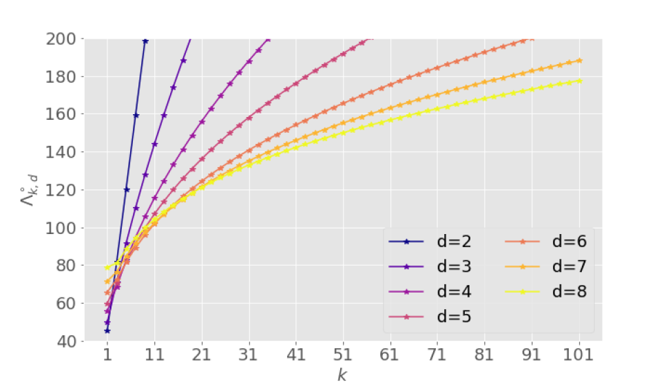
Figure 1. For indicated dimensions $d=1,\ldots,8$, a plot of $k$ vs. $\Lambda^{\circ}_{k,d}$.

$k\setminus d$	1	2	3	4	5	6	7	8
1,2	39.478	45.586	49.740	55.831	59.838	65.746	71.513	78.957
3,4	157.914	81.546	71.005	68.648	70.596	72.363	76.480	81.033
5,6	355.306	120.115	91.527	82.487	81.768	81.494	84.590	88.336
7,8	631.655	159.162	110.262	94.644	91.275	89.217	91.387	94.461
9,10	986.960	198.387	127.623	105.511	99.567	95.873	97.187	99.662
11,12	1421.223	237.697	143.920	115.401	106.966	101.748	102.262	104.187
13,14	1934.442	277.057	159.365	124.532	113.685	107.029	106.790	108.204
15,16	2526.619	316.446	174.109	133.050	119.864	111.845	110.892	111.826
17,18	3197.752	355.855	188.263	141.062	125.605	116.283	114.651	115.132
19,20	3947.842	395.279	201.909	148.649	130.981	120.410	118.128	118.179

Table 3. $\Lambda^{\circ}_{k,d}$ for the indicated values of the eigenvalue number $k$ and dimension $d$.

$k=1,2$	$k\geq 3$	lattice vector
1	1	0	0	0	0	0	0	0	$\lceil k/2\rceil$
2	2	0	0	0	0	0	0	1	0
3	3	0	0	0	0	0	0	1	1
4	4	0	0	0	0	0	1	0	0
5	5	0	0	0	0	0	1	1	0
6	6	0	0	0	0	0	1	1	1
7	7	0	0	0	0	1	0	0	0
8	8	0	0	0	0	1	0	-1	0
9	9	0	0	0	0	1	-1	-1	0
10	10	0	0	0	0	1	0	-1	-1
11	11	0	0	0	0	1	-1	-1	-1
12		0	0	0	0	1	-1	-2	-1
13	12	0	0	0	1	0	0	0	0
14	13	0	0	0	1	0	-1	0	0
15	14	0	0	0	1	1	-1	0	0
16	15	0	0	0	1	1	0	0	0
17	16	0	0	0	1	0	0	1	1
18	17	0	0	0	1	0	0	1	0
19	18	0	0	0	1	1	-1	-1	-1
20	19	0	0	0	1	1	-1	-1	0
21	20	0	0	1	0	0	0	0	0
22	21	0	0	1	-1	-1	1	0	0
23	22	0	0	1	0	-1	0	0	0
34	23	0	0	1	-1	-1	0	0	0
25	24	0	0	1	0	-1	0	1	1
26	25	0	0	1	0	-1	0	1	0
27	26	0	0	1	0	-1	1	1	1
28	27	0	0	1	-1	-1	1	1	1
29	28	0	0	1	0	-1	1	1	0
30	29	0	0	1	-1	-1	1	1	0
31	30	0	0	1	-1	-2	1	1	1
32	31	0	0	1	-1	-2	1	1	0
33		0	0	1	-1	-2	2	2	1
34		0	0	1	0	-1	1	2	1
35		0	0	1	0	-2	1	2	1
36		0	0	1	-1	-2	1	2	1
37	32	0	1	0	0	0	0	0	0
38	33	0	1	0	0	0	-1	-1	0
39	34	0	1	0	0	0	0	-1	0
40	35	0	1	0	-1	0	0	-1	0
41	36	0	1	0	0	1	0	-1	0
42	37	0	1	-1	0	1	0	-1	0
43	38	0	1	0	0	1	-1	-1	0
44	39	0	1	-1	0	1	-1	-1	0
45	40	0	1	0	1	1	-1	-1	0
46	41	0	1	-1	1	1	-1	-1	0
47	42	0	1	-1	1	2	-1	-1	0
48	43	0	1	0	0	1	-1	-2	0
49	44	0	1	-1	0	1	-1	-2	0
50	45	0	1	0	0	1	-1	-2	-1
51	46	0	1	-1	0	1	-1	-2	-1
52	47	0	1	-1	1	2	-2	-2	0
53	48	0	1	-1	1	2	-2	-2	-1
54	49	0	1	0	0	0	0	0	1
55	50	0	1	-1	0	2	-1	-2	0
56	51	0	1	-1	1	2	-1	-2	0
57	52	0	1	-1	0	2	-1	-2	-1
58	53	0	1	-1	1	2	-1	-2	-1
59		0	1	-2	1	3	-2	-3	-1
60		0	1	-1	1	2	-2	-3	-1

$k=1,2$	$k\geq 3$	lattice vector
61		0	1	-1	0	2	-2	-3	-1
62		0	1	-1	0	2	-1	-3	-1
63		0	1	-1	1	3	-2	-3	-1
64	54	1	0	0	0	0	0	0	0
65	55	1	0	0	-1	-1	0	-1	0
66	56	1	0	0	0	0	-1	-1	0
67	57	1	1	-1	0	1	-1	-2	0
68	58	1	0	0	0	0	0	-1	0
69	59	1	0	0	-1	0	0	-1	0
70	60	1	0	-1	0	0	-1	-1	0
71	61	1	-1	0	-1	-1	1	0	0
72	62	1	-1	0	0	-1	0	0	0
73	63	1	-1	0	-1	-1	0	0	0
74	64	1	0	-1	0	0	0	-1	0
75	65	1	0	-1	-1	0	0	-1	0
76	66	1	-1	-1	0	0	0	0	0
77	67	1	-1	0	0	0	0	0	0
78	68	1	0	-1	0	1	0	-1	0
79	69	1	0	-1	0	1	-1	-1	0
80	70	1	0	-1	1	1	-1	-1	0
81	71	1	-1	0	-1	-2	1	1	0
82	72	1	-1	0	0	-1	0	1	0
83	73	1	-1	0	0	-1	0	1	1
84	74	1	0	-1	0	1	-1	-2	-1
85	75	1	0	-1	0	1	-1	-2	0
86	76	1	-1	0	0	-1	1	1	0
87	77	1	-1	0	-1	-1	1	1	0
88	78	1	-1	0	0	-1	1	1	1
89	79	1	-1	0	-1	-1	1	1	1
90	80	1	0	0	-1	-1	1	0	0
91	81	1	-1	0	-1	-2	1	1	1
92	82	1	0	0	0	-1	0	0	0
93	83	1	0	0	-1	-1	0	0	0
94	84	1	0	0	0	0	0	0	1
95	85	1	0	-1	0	0	0	0	0
96	86	1	0	0	-1	-1	1	0	1
97	87	1	0	0	0	-1	0	0	1
98	88	1	0	0	-1	-1	0	0	1
99	89	1	0	-1	0	0	0	0	1
100	90	1	-1	1	-1	-2	1	1	0
101	91	1	-1	1	-1	-2	1	1	1
102		1	-1	0	0	-1	1	2	1
103		1	-1	1	-1	-3	2	2	1
104		1	-1	1	-2	-3	2	2	1
105		1	-1	0	0	-2	1	2	1
106		1	0	1	-1	-2	1	1	1
107		1	-1	0	-1	-2	2	2	1
108		1	0	0	0	-1	0	1	1
109		1	-1	1	0	-2	1	2	1
110		1	0	0	-1	-2	1	1	1
111		1	0	0	-1	-1	1	1	1
112		1	-1	1	-1	-3	2	3	1
113		1	-2	1	-1	-3	2	3	1
114		1	-1	1	-1	-3	2	3	2
115		1	-1	1	-1	-2	2	2	1
116		1	-1	1	-1	-3	1	2	1
117		1	0	0	0	-1	1	1	1
118		1	-1	0	-1	-2	1	2	1
119		1	-1	1	-1	-2	1	2	1
120		2	-1	0	-1	-2	1	1	1

Table 4. For the $B^{\circ}_{k,d}$-lattice, $k$-th shortest lattice vectors and indexing for $k=1,2$ and $k\geq 3$. For $d<8$, as indicated by horizontal lines, we use only vectors that are zero in the first $8-d$ components. The red indices are discussed in Section 4.2.

2. Comments on the computations supporting Numerical Observation 1.2

Here, we discuss the claims in Numerical Observation 1.2 regarding the $k$-th volume-normalized Laplacian eigenvalues of the torus $T^{\circ}_{k,d}$,

(9) $$\Lambda^{\circ}_{k,d}:=\min_{E\in\mathbb{Z}^{d}_{k+1}}\ \max_{v\in E}\ 4\pi^{2}(\det B^{\circ}_{k,d})^{\frac{2}{d}}\|(B^{\circ}_{k,d})^{-t}v\|^{2}.\qquad$$

and the corresponding lattice vectors, $E$. For $k=1$, the computation of $\Lambda^{\circ}_{k,d}$ is known as the shortest lattice vector problem (SVP) for the dual lattice, $\Gamma^{*}_{B^{\circ}_{k,d}}=(B^{\circ}_{k,d})^{-t}\mathbb{Z}^{d}$. The SVP appears in a variety of cryptoanalysis problems and, although NP-hard [1, 20], can be solved for fixed k in moderately-high dimensions [11, 19]. We are unaware of a method to find the shortest $k$ vectors of the lattice $B^{\circ}_{k,d}$ analytically.

For fixed (small to moderately large) $k\in\mathbb{N}$ , we can compute $\Lambda^{\circ}_{k,d}$ in a rigorous way using the ShortVectors function in Magma [5]. The enumeration routine underlying this function relies on floating-point approximation, but is run in a rigorous way by using the default setting with the parameter Proof set to true. For each $d=1,\ldots,8$, we checked all values of $k$ from 1 to 500,000 and every value $k\in\{1\times 10^{6},\ 2\times 10^{6},\ \cdots,\ 9\times 10^{6},\ 1\times 10^{7},\ 2\times 10^{7},\ \cdots,\ 9\times 10^{7},\ 1\times 10^{8}\}$. Magma code with these supporting computations can be found in the solve_SVP.magma file at [13]. Indeed, the claims made in Numerical Observation 1.2 hold for these values of $k$.

3. Eigenvalue perturbation formulae and conditions for stationarity

Recall that the eigenvalues of $-\Delta$ on a flat torus each have multiplicity of at least two. We will refer to an eigenvalue as a double eigenvalue if it has multiplicity of exactly two. We first give the perturbation formula for a double eigenvalue.

Theorem 3.1.

When $\lambda$ is a double eigenvalue with corresponding lattice vectors $\pm v\in\mathbb{Z}^{d}$, the variation of the normalized eigenvalue $\Lambda$ with respect to the Gram matrix $G$ satisfies

$$\Lambda\left(G_{0}+\delta G\right)=\Lambda\left(G_{0}\right)+\left\langle\frac{\partial\Lambda}{\partial G},\delta G\right\rangle_{F}+o\left(\left\|\delta G\right\|\right)$$

where $\frac{\partial\Lambda}{\partial G}=-\frac{\Lambda}{d}G^{-1}+4\pi^{2}\left(\det(G)\right)^{-\frac{1}{d}}vv^{t}$.

Proof.

For an invertible, symmetric matrix $G$, Jacobi’s formula states that

$$\det(G_{0}+\delta G)=\det G_{0}+\det G_{0}\langle G^{-1},\delta G\rangle+o\left(\left\|\delta G\right\|\right).$$

Since

$$\Lambda=4\pi^{2}\left(\det(G)\right)^{-\frac{1}{d}}\left\langle vv^{t},G\right\rangle_{F},$$

for fixed lattice vector $v$, we obtain the desired result using the product rule. ∎

We next give a perturbation formula for eigenvalues of greater multiplicity.

Theorem 3.2.

Suppose the Laplacian eigenvalue $\lambda$ has even multiplicity $m>2$ with corresponding lattice vectors given by $\pm v_{j}\in\mathbb{Z}^{d}$, $j=1,\ldots,\frac{m}{2}$. A perturbation of the Gram matrix of the form $G=G_{0}+\delta G$ will split the normalized eigenvalue $\Lambda=|\det G|^{-\frac{1}{d}}\lambda$ into up to $\frac{m}{2}$ (un-sorted) normalized eigenvalues (each with multiplicity of at least two) given by

$$\Lambda_{j}\left(G_{0}+\delta G\right)=\Lambda\left(G_{0}\right)+\mu_{j}+o\left(\left\|\delta G\right\|\right),\qquad\qquad j=1,\ldots,\frac{m}{2}$$

where $\mu_{j}=\langle M_{j},\delta G\rangle$ and

(10) $$M_{j}=-\frac{\Lambda}{d}G_{0}^{-1}+4\pi^{2}\left(\det G_{0}\right)^{-\frac{1}{d}}v_{j}v_{j}^{t}.$$

Proof.

The volume-normalized eigenvalue, $\Lambda$, satisfies

$$4\pi^{2}\left(\det(G_{0})\right)^{-\frac{1}{d}}\left\langle v_{j},G_{0}v_{j}\right\rangle=\Lambda,\qquad\qquad 1\leq j\leq\frac{m}{2}.$$

Noting that the lattice vectors $v_{j}$ are fixed, the perturbed volume normalized eigenvalues satisfy

$$4\pi^{2}\left(\det(G_{0}+\delta G)\right)^{-\frac{1}{d}}\left\langle v_{j},(G_{0}+\delta G)v_{j}\right\rangle=\Lambda+\mu_{j}+o(\|\delta G\|),\qquad\qquad 1\leq j\leq\frac{m}{2}.$$

The first order terms give

$$-\frac{4\pi^{2}}{d}\left(\det(G_{0})\right)^{-\frac{1}{d}}\,\langle G_{0}^{-1},\delta G\rangle\left\langle v_{j},G_{0}v_{j}\right\rangle+4\pi^{2}\left(\det(G_{0})\right)^{-\frac{1}{d}}\left\langle v_{j},\delta Gv_{j}\right\rangle=\mu_{j},\qquad\qquad 1\leq j\leq\frac{m}{2}.$$

Thus

$$\mu_{j} =4\pi^{2}\left(\det(G_{0})\right)^{-\frac{1}{d}}\left\{\left\langle v_{j},\delta Gv_{j}\right\rangle-\frac{1}{d}\langle G_{0}^{-1},\delta G\rangle\left\langle v_{j},G_{0}v_{j}\right\rangle\right\},$$

as desired. ∎

Recall that the volume normalized eigenvalue is scale invariant, i.e., $\Lambda(\alpha G_{0})=\Lambda(G_{0})$ for $\alpha\neq 0$. In Theorem 3.2, if we take $\delta G=\varepsilon G_{0}$ we obtain $\mu_{j}=0$ for all $j=1,\ldots,\frac{m}{2}$ and $\Lambda_{j}(G_{0}+\delta G)=\Lambda(G_{0})+o(\|G_{0}\|)$, as we expect.

We next use Theorem 3.2 to derive two necessary conditions for local optimality in the eigenvalue optimization problem (4). We say that $G_{0}$ is a stationary point for $\Lambda$ if for every $\delta G$ we have that there exists at least one $j\in\{1,\ldots,\frac{m}{2}\}$ such that $\mu_{j}\leq 0$. We say that $G_{0}$ is a strict local maximum for $\Lambda$ if for every $\delta G$ satisfying $\langle\delta G,G_{0}\rangle=0$ we have at least one $j\in\{1,\ldots,\frac{m}{2}\}$ such that $\mu_{j}<0$.

Theorem 3.3.

Using the notation in Theorem 3.2, a necessary condition for $G_{0}$ to be a strict local maximum for $\Lambda$ is that the collection of outer products $\{v_{j}v_{j}^{t}\}_{j=1}^{\frac{m}{2}}$ spans the space of symmetric $\mathbb{R}^{d\times d}$ matrices.

Proof.

Otherwise, there exists a matrix $\delta G=A$ so that for all $j=1,\ldots,\frac{m}{2}$, we have

$$\langle A,v_{j}v_{j}^{t}\rangle=0.$$

In this case, for every $j=1,\ldots,\frac{m}{2}$, we have

$$\mu_{j}=\langle M_{j},A\rangle=-\frac{\Lambda}{d}\langle G_{0}^{-1},A\rangle.$$

Changing the sign of $A$ if necessary, we may assume that $\langle G_{0}^{-1},A\rangle\leq 0$, implying $\mu_{j}\geq 0$ for all $j=1,\ldots,\frac{m}{2}$. ∎

Theorem 3.4.

Using the notation in Theorem 3.2, the Gram matrix $G_{0}$ is a stationary point for $\Lambda$ if and only if there are non-negative coefficients $c_{j}\geq 0$, $j=1,\ldots,\frac{m}{2}$, not all zero, such that $\sum_{j=1}^{\frac{m}{2}}c_{j}M_{j}=0$.

Proof.

We consider the linear map $U\colon\mathbb{S}^{d}_{++}\to\mathbb{R}^{\frac{m}{2}}$ defined by

$$U_{j}(G):=\mu_{j}(G)=\langle M_{j},G\rangle_{F},\qquad\qquad j=1,\ldots,\frac{m}{2}.$$

To find the adjoint map of $U$, denoted $U^{*}\colon\mathbb{R}^{\frac{m}{2}}\to\mathbb{S}^{d}_{++}$, for $c\in\mathbb{R}^{\frac{m}{2}}$, we compute

$$\langle U_{j}(G),c\rangle_{\mathbb{R}^{\frac{m}{2}}}=\sum_{j=1}^{\frac{m}{2}}c_{j}\langle M_{j},G\rangle_{F}=\left\langle\left(\sum_{j=1}^{\frac{m}{2}}c_{j}M_{j}\right),G\right\rangle_{F},$$

so that $U^{*}c=\sum_{j=1}^{\frac{m}{2}}c_{j}M_{j}$.

Stationarity of $G_{0}$ means that $\delta G\mapsto U(\delta G)\in\mathbb{R}^{\frac{m}{2}}$ has at least one non-positive component for every $\delta G$, i.e., there is no solution to the linear system

(11) $$U(\delta G)>0.$$

We recall Gordan’s Alternative Theorem (see, e.g., [2, Thm. 10.4]) which states that either (11) has a solution or

(12) $$U^{*}c=0,\quad c\geq 0,\ c\neq 0$$

has a solution. Thus it is enough to show that there is a non-trivial, non-negative $c\in\textrm{ker}(U^{*})$. ∎

Remark 3.5.

For $k=1$, the eigenvalue optimization problem (4) is equivalent to Hermite’s constant (7) and determining the densest lattice sphere packing. It was shown by Voronoi that a lattice gives the densest lattice sphere packing if and only if it is perfect and eutactic [24, Thm. 3.9]. It can be seen that the necessary conditions here imply Theorems 3.3 and 3.4 for $k=1$. Note that the lack of convexity for higher eigenvalues makes a sufficiency condition more difficult to state.

4. Properties of flat tori, $T^{\circ}_{k,d}$, and degeneracy as $k\to\infty$

In this section, we show that $G^{\circ}_{k,d}$ for $d\leq 8$ and $k\geq 1$ satisfies the necessary condition for strict local maximum given in Theorem 3.3 (see Section 4.1) and provide numerical evidence that it satisfies the necessary condition for stationarity in Theorem 3.4 (see Section 4.2). In Section 4.3, we describe the degeneracy of flat tori $T^{\circ}_{k,d}$ as $k\to\infty$.

4.1. Linear Independence

Theorem 4.1.

Let $\{v_{j}\}_{j=1}^{\frac{m}{2}}$ be the collection of lattice vectors gives in Table 4. The collection of outer products $\{v_{j}v_{j}^{t}\}_{j=1}^{\frac{m}{2}}$ spans the space of symmetric $\mathbb{R}^{d\times d}$ matrices. Consequently, $G^{\circ}_{k,d}$ for $d\leq 8$ and $k\geq 1$ satisfy the necessary conditions for a strict local maximum given in Theorem 3.3.

Proof.

We only need $\binom{d}{2}\leq\frac{m}{2}$ outer products $v_{j}v_{j}^{t}$ to span the space of symmetric matrices, so for dimensions, $d=4,5,6,7,8$, it is not necessary to use all of the lattice vectors listed in Table 4. The lattice vector indices we use are given by

$$J=\{1\mid 2,3\mid 4:6\mid 7:10\mid 12:14,16,17\mid 20:25\mid 32:37,49\mid 54,56,64,66,67,82,83,84\}.$$

Here, the vertical lines correspond to the horizontal lines in Table 4 and identify the dimension that the lattice vector first appears. For each dimension $d$, we reshape the upper triangular part of the matrices $v_{j}v_{j}^{t}$ into vectors and stacking the vectors as columns of a matrix $F_{d}\in\mathbb{R}^{\binom{d}{2}\times\binom{d}{2}}$. The matrices $F_{d}$ are the lower left $\binom{d}{2}\times\binom{d}{2}$ block of the following matrix, $F\in\mathbb{R}^{36\times 36}$, where to reduce size we use the shorthand $\blacktriangle=1$, $\blacktriangledown=-1$, and $\blacksquare=\frac{\kappa^{2}}{4}$,

$$F=\left[\begin{array}[]{r|rr|rrr|rrrr|rrrrr|rrrrrr|rrrrrrr|rrrrrrrr}0&0&0&0&0&0&0&0&0&0&0&0&0&0&0&0&0&0&0&0&0&0&0&0&0&0&0&0&\blacktriangle&\blacktriangle&\blacktriangle&\blacktriangle&\blacktriangle&\blacktriangle&\blacktriangle&\blacktriangle\\ 0&0&0&0&0&0&0&0&0&0&0&0&0&0&0&0&0&0&0&0&0&0&0&0&0&0&0&0&0&0&0&\blacktriangledown&\blacktriangledown&0&0&0\\ 0&0&0&0&0&0&0&0&0&0&0&0&0&0&0&0&0&0&0&0&0&0&0&0&0&0&0&0&0&0&\blacktriangledown&\blacktriangledown&0&0&0&0\\ 0&0&0&0&0&0&0&0&0&0&0&0&0&0&0&0&0&0&0&0&0&0&0&0&0&0&0&0&0&0&0&0&0&0&\blacktriangledown&0\\ 0&0&0&0&0&0&0&0&0&0&0&0&0&0&0&0&0&0&0&0&0&0&0&0&0&0&0&0&0&0&0&0&0&\blacktriangledown&\blacktriangledown&0\\ 0&0&0&0&0&0&0&0&0&0&0&0&0&0&0&0&0&0&0&0&0&0&0&0&0&0&0&0&0&\blacktriangledown&0&0&0&0&0&0\\ 0&0&0&0&0&0&0&0&0&0&0&0&0&0&0&0&0&0&0&0&0&0&0&0&0&0&0&0&0&\blacktriangledown&\blacktriangledown&0&0&0&0&0\\ 0&0&0&0&0&0&0&0&0&0&0&0&0&0&0&0&0&0&0&0&0&0&0&0&0&0&0&0&0&0&0&0&0&0&0&\blacktriangle\\ \hline\cr 0&0&0&0&0&0&0&0&0&0&0&0&0&0&0&0&0&0&0&0&0&\blacktriangle&\blacktriangle&\blacktriangle&\blacktriangle&\blacktriangle&\blacktriangle&\blacktriangle&0&0&0&\blacktriangle&\blacktriangle&0&0&0\\ 0&0&0&0&0&0&0&0&0&0&0&0&0&0&0&0&0&0&0&0&0&0&0&0&0&0&\blacktriangledown&0&0&0&0&\blacktriangle&0&0&0&0\\ 0&0&0&0&0&0&0&0&0&0&0&0&0&0&0&0&0&0&0&0&0&0&0&0&\blacktriangledown&0&0&0&0&0&0&0&0&0&0&0\\ 0&0&0&0&0&0&0&0&0&0&0&0&0&0&0&0&0&0&0&0&0&0&0&0&0&\blacktriangle&\blacktriangle&0&0&0&0&0&0&0&0&0\\ 0&0&0&0&0&0&0&0&0&0&0&0&0&0&0&0&0&0&0&0&0&0&\blacktriangledown&0&0&0&0&0&0&0&0&0&0&0&0&0\\ 0&0&0&0&0&0&0&0&0&0&0&0&0&0&0&0&0&0&0&0&0&0&\blacktriangledown&\blacktriangledown&\blacktriangledown&\blacktriangledown&\blacktriangledown&0&0&0&0&0&0&0&0&0\\ 0&0&0&0&0&0&0&0&0&0&0&0&0&0&0&0&0&0&0&0&0&0&0&0&0&0&0&\blacktriangle&0&0&0&0&0&0&0&0\\ \hline\cr 0&0&0&0&0&0&0&0&0&0&0&0&0&0&0&\blacktriangle&\blacktriangle&\blacktriangle&\blacktriangle&\blacktriangle&\blacktriangle&0&0&0&0&0&\blacktriangle&0&0&0&\blacktriangle&\blacktriangle&0&0&0&0\\ 0&0&0&0&0&0&0&0&0&0&0&0&0&0&0&0&\blacktriangledown&0&\blacktriangledown&0&0&0&0&0&0&0&0&0&0&0&0&0&0&0&0&0\\ 0&0&0&0&0&0&0&0&0&0&0&0&0&0&0&0&\blacktriangledown&\blacktriangledown&\blacktriangledown&\blacktriangledown&\blacktriangledown&0&0&0&0&0&\blacktriangledown&0&0&0&0&0&0&0&0&0\\ 0&0&0&0&0&0&0&0&0&0&0&0&0&0&0&0&\blacktriangle&0&0&0&0&0&0&0&0&0&0&0&0&0&0&0&0&0&0&0\\ 0&0&0&0&0&0&0&0&0&0&0&0&0&0&0&0&0&0&0&\blacktriangle&\blacktriangle&0&0&0&0&0&\blacktriangle&0&0&0&\blacktriangle&0&0&0&0&0\\ 0&0&0&0&0&0&0&0&0&0&0&0&0&0&0&0&0&0&0&\blacktriangle&0&0&0&0&0&0&0&0&0&0&0&0&0&0&0&0\\ \hline\cr 0&0&0&0&0&0&0&0&0&0&\blacktriangle&\blacktriangle&\blacktriangle&\blacktriangle&\blacktriangle&0&\blacktriangle&0&\blacktriangle&0&0&0&0&0&\blacktriangle&0&0&0&0&0&0&0&0&0&\blacktriangle&0\\ 0&0&0&0&0&0&0&0&0&0&0&0&\blacktriangle&0&0&0&\blacktriangle&0&\blacktriangle&0&0&0&0&0&0&0&0&0&0&0&0&0&0&0&\blacktriangle&0\\ 0&0&0&0&0&0&0&0&0&0&0&\blacktriangledown&\blacktriangledown&0&0&0&\blacktriangledown&0&0&0&0&0&0&0&0&0&0&0&0&0&0&0&0&0&0&0\\ 0&0&0&0&0&0&0&0&0&0&0&0&0&\blacktriangle&\blacktriangle&0&0&0&0&0&0&0&0&0&\blacktriangle&0&0&0&0&0&0&0&0&0&0&0\\ 0&0&0&0&0&0&0&0&0&0&0&0&0&\blacktriangle&0&0&0&0&0&0&0&0&0&0&0&0&0&0&0&0&0&0&0&0&0&0\\ \hline\cr 0&0&0&0&0&0&\blacktriangle&\blacktriangle&\blacktriangle&\blacktriangle&0&0&\blacktriangle&0&0&0&\blacktriangle&\blacktriangle&\blacktriangle&\blacktriangle&\blacktriangle&0&0&0&0&\blacktriangle&\blacktriangle&0&0&0&0&0&0&\blacktriangle&\blacktriangle&0\\ 0&0&0&0&0&0&0&0&\blacktriangledown&0&0&0&\blacktriangledown&0&0&0&\blacktriangledown&0&0&0&0&0&0&0&0&0&0&0&0&0&0&0&0&0&0&0\\ 0&0&0&0&0&0&0&\blacktriangledown&\blacktriangledown&\blacktriangledown&0&0&0&0&0&0&0&0&0&\blacktriangledown&\blacktriangledown&0&0&0&0&\blacktriangledown&\blacktriangledown&0&0&0&0&0&0&0&0&0\\ 0&0&0&0&0&0&0&0&0&\blacktriangledown&0&0&0&0&0&0&0&0&0&\blacktriangledown&0&0&0&0&0&0&0&0&0&0&0&0&0&0&0&0\\ \hline\cr 0&0&0&\blacktriangle&\blacktriangle&\blacktriangle&0&0&\blacktriangle&0&0&\blacktriangle&\blacktriangle&0&0&0&\blacktriangle&0&0&0&0&0&\blacktriangle&0&0&0&0&0&0&\blacktriangle&0&0&0&0&0&0\\ 0&0&0&0&\blacktriangle&\blacktriangle&0&0&\blacktriangle&0&0&0&0&0&0&0&0&0&0&0&0&0&\blacktriangle&0&0&0&0&0&0&\blacktriangle&0&0&0&0&0&0\\ 0&0&0&0&0&\blacktriangle&0&0&0&0&0&0&0&0&0&0&0&0&0&0&0&0&0&0&0&0&0&0&0&0&0&0&0&0&0&0\\ \hline\cr 0&\blacktriangle&\blacktriangle&0&\blacktriangle&\blacktriangle&0&\blacktriangle&\blacktriangle&\blacktriangle&0&0&0&\blacktriangle&\blacktriangle&0&0&0&0&\blacktriangle&\blacktriangle&0&\blacktriangle&\blacktriangle&\blacktriangle&\blacktriangle&\blacktriangle&0&0&\blacktriangle&\blacktriangle&0&0&0&0&0\\ 0&0&\blacktriangle&0&0&\blacktriangle&0&0&0&\blacktriangle&0&0&0&\blacktriangle&0&0&0&0&0&\blacktriangle&0&0&0&0&0&0&0&0&0&0&0&0&0&0&0&0\\ \hline\cr\blacksquare&0&\blacktriangle&0&0&\blacktriangle&0&0&0&\blacktriangle&0&0&0&\blacktriangle&0&0&0&0&0&\blacktriangle&0&0&0&0&0&0&0&\blacktriangle&0&0&0&0&0&0&0&\blacktriangle\end{array}\right].$$

We will show that the matrices $F_{d}$ have non-zero determinant, and hence the outer products are linearly independent. If the matrix $F$ has non-zero determinant, then $F_{d}$ for each $d\leq 8$ also has non-zero determinant. Observing that the upper left submatrix blocks of $F$ are zero, we see that the determinant of $F$ is the product of the lower-left to upper-right diagonal sub-blocks of the matrix $F$. Judiciously choosing the minors in the Laplace expansion for the determinant, we obtain $|\det F|=|\det F_{d}|=\frac{\kappa^{2}}{4}\neq 0$. ∎

4.2. Stationarity of tori

Here, for each $k\geq 1$ and $2\leq d\leq 8$, we give a vector $c=c(k,d)\in\mathbb{R}^{\frac{m}{2}}$, that satisfies the stationarity condition given in Theorem 3.4. We first observe that such a vector $c$, if one exists, is not unique for $d=4,5,6,7,8$, as the following argument shows. Reshaping the symmetric matrices $M_{j}$ as defined in (10) into vectors of length $\binom{d}{2}$, the condition for stationarity in Theorem 3.4 is that a non-negative linear combination gives zero. Of course, if the number of vectors, $\frac{m}{2}$, exceeds $\binom{d}{2}$, i.e., $m>d(d+1)$, then the columns are linearly dependent. Looking at Table 2, this is the case for d = 4,5,6,7,8.

$d$	2	3	4	5	6	7	8
$a_{k,d}$	$\frac{2\kappa^{2}-4}{\kappa^{2}}$	$\frac{3\kappa^{2}-8}{\kappa^{2}}$	$4\frac{\kappa^{2}-4}{\kappa^{2}}$	$6\frac{\kappa^{2}-4}{\kappa^{2}}$	$8\frac{\kappa^{2}-5}{\kappa^{2}}$	$4\frac{3\kappa^{2}-16}{\kappa^{2}}$	$18\frac{\kappa^{2}-6}{\kappa^{2}}$
$b_{k,d}$	$\cdot$	$\frac{2\kappa^{2}-4}{\kappa^{2}}$	$2\frac{\kappa^{2}-4}{\kappa^{2}}$	$2\frac{\kappa^{2}-3}{\kappa^{2}}$	$2\frac{\kappa^{2}-4}{\kappa^{2}}$	$2\frac{\kappa^{2}-4}{\kappa^{2}}$	$\frac{2\kappa^{2}-9}{\kappa^{2}}$

Table 5. The values of $a_{k,d}$ and $b_{k,d}$ used in the definition of the vector $c^{\circ}$. See Section 4.2.

For $k=1,2$, for every $2\leq d\leq 8$, define $c^{\circ}=(1,\cdots,1)\in\mathbb{R}^{\frac{m}{2}}$. For $k\geq 3$ and $2\leq d\leq 8$, define the vector $c^{\circ}\in\mathbb{R}^{\frac{m}{2}}$ by

$$c^{\circ}_{i}=\begin{cases}a_{k,d}&i=1\\ b_{k,d}&i\in I\\ 1&\textrm{otherwise},\end{cases}$$

where the constants $a_{k,d}$ and $b_{k,d}$ are specified in Table 5 and the index set $I$ is defined

$$I:=\{ 4\mid 7\mid 12:15\mid 20:23\mid 33:42\mid 55:70\}.$$

The indices in $I$ correspond to the lattice vectors in Table 4, where the indices in $I$ are displayed in red. The vertical lines here correspond to the horizontal lines in Table 4 and identify the dimension that the lattice vector first appears.

Numerical Observation 4.2.

For every $k\geq 1$, and $2\leq d\leq 8$, the vector $c^{\circ}\in\mathbb{R}^{\frac{m}{2}}$ satisfies the stationarity condition given in Theorem 3.4.

It is straightforward to check that Numerical Observation 4.2 holds. Sage code that symbolically verifies the claim is provided in [13]. Comments on how we first identified $c^{\circ}\in\mathbb{R}^{\frac{m}{2}}$ are made in Appendix A.2.

As an example, we verify Numerical Observation 4.2 in dimension $d=3$. We have $G^{\circ}_{k,d}=\begin{pmatrix}2\kappa^{2}&-\kappa^{2}&0\\ -\kappa^{2}&2\kappa^{2}&-4\\ 0&-4&8\kappa^{2}\end{pmatrix}$ so that

$$(G^{\circ}_{k,d})^{-1}=\frac{1}{8(3\kappa^{2}-4)}\begin{pmatrix}16\frac{\kappa^{2}-1}{\kappa^{2}}&8&4\\ 8&16&8\\ 4&8&3\kappa^{2}\end{pmatrix},$$

and $\det G^{\circ}_{k,d}=8\kappa^{2}(3\kappa^{2}-4)$. We also have $\Lambda^{\circ}_{k,3}=4\pi^{2}\left(\frac{\kappa^{4}}{3\kappa^{2}-4}\right)^{\frac{1}{3}}=8\pi^{2}\kappa^{2}\left(\det G^{\circ}_{k,d}\right)^{-1/d}$ (see Table 2), and, from Table 4 and Table 5,

$$c_{1}^{\circ} =\frac{3\kappa^{2}-8}{\kappa^{2}} v_{1}v_{1}^{t}=\begin{pmatrix}0&0&0\\ 0&0&0\\ 0&0&\frac{\kappa^{2}}{4}\end{pmatrix}$$

$$c_{2}^{\circ} =1 v_{2}v_{2}^{t}=\begin{pmatrix}0&0&0\\ 0&1&0\\ 0&0&0\end{pmatrix}$$

$$c_{3}^{\circ} =1 v_{3}v_{3}^{t}=\begin{pmatrix}0&0&0\\ 0&1&1\\ 0&1&1\end{pmatrix}$$

$$c_{4}^{\circ} =\frac{2\kappa^{2}-4}{\kappa^{2}} v_{4}v_{4}^{t}=\begin{pmatrix}1&0&0\\ 0&0&0\\ 0&0&0\end{pmatrix}$$

$$c_{5}^{\circ} =1 v_{5}v_{5}^{t}=\begin{pmatrix}1&1&0\\ 1&1&0\\ 0&0&0\end{pmatrix}$$

$$c_{6}^{\circ} =1 v_{6}v_{6}^{t}=\begin{pmatrix}1&1&1\\ 1&1&1\\ 1&1&1\end{pmatrix}.$$

We can then compute

$$\sum_{i=1}^{6}c_{i}^{\circ}M_{i} =-\frac{\Lambda^{\circ}_{k,3}}{d}\left(\sum_{i=1}^{6}c_{i}^{\circ}\right)(G^{\circ}_{k,d})^{-1}+4\pi^{2}\left(\det G^{\circ}_{k,d}\right)^{-\frac{1}{d}}\sum_{i=1}^{6}c_{i}^{\circ}v_{i}v_{i}^{t}.$$

Since $\sum_{i=1}^{6}c_{i}^{\circ}=3\left(\frac{3\kappa^{2}-4}{\kappa^{2}}\right)$ and

$$\sum_{i=1}^{6}c_{i}^{\circ}v_{i}v_{i}^{t}=\begin{pmatrix}4(\kappa^{2}-1)/\kappa^{2}&2&1\\ 2&4&2\\ 1&2&3\kappa^{2}/4\end{pmatrix},$$

we obtain $\sum_{i=1}^{6}c_{i}^{\circ}M_{i}=0$.

4.3. Degeneracy of flat tori as $k\to\infty$

For fixed $k\in\mathbb{N}$ and $d\leq 8$, denote the eigenvalues of the normalized Gram matrix $\frac{G_{k,d}^{\circ}}{\textrm{det}\left(G_{k,d}^{\circ}\right)^{\frac{1}{d}}}$ by $\mu^{k}_{1}\leq\mu^{k}_{2}\leq\cdots\leq\mu^{k}_{d}$. In Figure 2, we plot $k$ vs $\mu^{k}_{1},\ldots,\mu^{k}_{d}$ for $d=2,\ldots,8$. From Figure 2, we hypothesize that, in each dimension, for large $k$,

$$\mu_{i}^{k}\sim c_{i}k^{2\cdot p_{i}/d},$$

for constants $c_{i},p_{i}$ that are independent of $k$. In particular, $p_{1}=-(d-1)$ and $p_{2}=\cdots=p_{d}=1$, which necessarily satisfy $\sum_{i=1}^{d}p_{i}=0$.

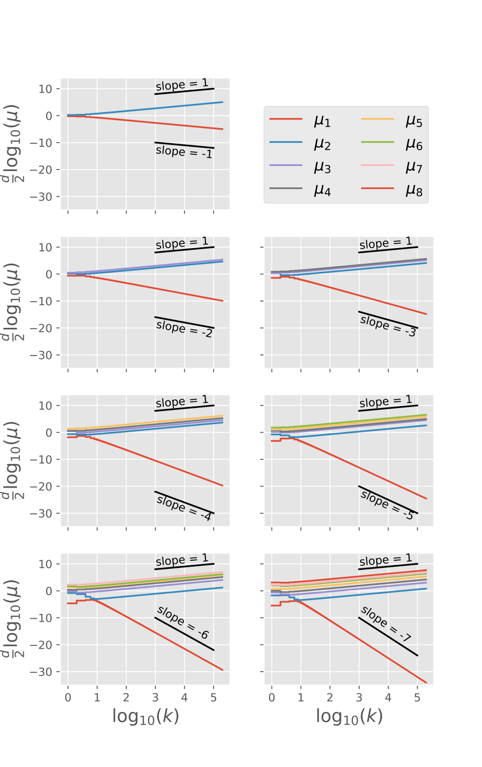
Figure 2. Log-log plots of $k$ vs the eigevalues, $\mu$, of the Gram matrix, $G_{k,d}^{\circ}$ for dimensions $d=2,\ldots,8$.

In Figure 3, we give further geometric interpretation of $v^{t}G^{\circ}_{k,d}v=2\kappa^{2}$ in dimensions $d=2$ and $3$. For $k=1,3,5,7$, we plot the ellipses/ellipsoids corresponding to the Gram matrix, as well as the $k$-th shortest lattice vectors. In $d=2$ dimensions, the ellipses intersect six lattice points and elongate as $k$ increases in one direction. In $d=3$ dimensions, the ellipsoids intersect 12 lattice points and again elongate in one direction. In both cases, the elongation in one direction corresponds to the first eigenvalue of the Gram matrix scaling as $\mu_{1}(k)\sim c_{1}k^{-2(d-1)/d}$ and the other eigenvalues scaling as $\mu_{i}(k)\sim c_{i}k^{2/d}$.

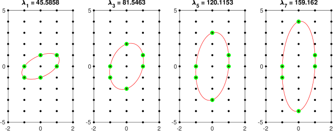
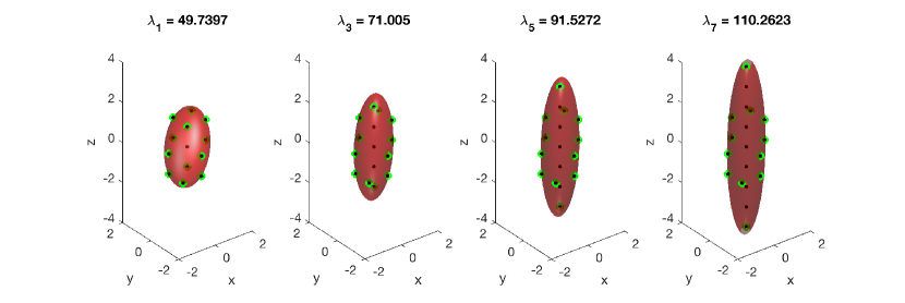
Figure 3. The ellipses ($d=2$) and ellipsoids ($d=3$) corresponding to the Gram matrix, $G_{k,d}^{\circ}$ for $k=1,3,5,7$. The intersecting lattice points are indicated.

Finally, we conclude with a discussion of the successive minima. Recall that, for $1\leq i\leq d$, the $i$-th successive minimum of a lattice with basis $B$ is defined by

$$\gamma_{i}(B)=\min\{\|v_{i}\|\colon\exists\textrm{ lin. ind. }v_{1}\ldots,v_{i}\in B\mathbb{Z}^{d}\textrm{ with }\|v_{1}\|\leq\ldots\leq\|v_{i}\|\}.$$

That is, $\gamma_{i}$ is the smallest number $\gamma$, such that the ellipsoid $\{\|Bx\|\leq\gamma\}$ contains $i$ linearly independent vectors (see, e.g., [24]). For each $k\geq 1$, $d\leq 8$, we have $\gamma_{1}((B^{\circ}_{k,d})^{-t})=2\sqrt{2}$ is attained by the vector $(0,\cdots,1)$ and $\gamma_{2}((B^{\circ}_{k,d})^{-t})=\cdots=\gamma_{d}((B^{\circ}_{k,d})^{-t})=\sqrt{2}\kappa$. In particular, since the injectivity radius of a flat torus, $T_{B}$, satisfies $\textrm{inj}(T_{B})=\gamma_{1}(B)\asymp\gamma_{d}(B^{-t})^{-1}$, we have that $\textrm{inj}(T_{k,d}^{\circ})\asymp k^{-1}$. If we scale $T_{k,d}^{\circ}$ by $\alpha=\textrm{vol}(T_{k,d}^{\circ})^{-\frac{1}{d}}=|\det G_{k,d}^{\circ}|^{\frac{1}{2d}}\asymp k^{\frac{d-1}{d}}$ (see Table 2), we obtain that $\textrm{vol}(\alpha T_{k,d}^{\circ})=1$. We then compute $\textrm{inj}(\alpha T_{k,d}^{\circ})=\gamma_{1}(\alpha B)=\alpha\gamma_{1}(B)\asymp\alpha\gamma_{d}(B^{-t})^{-1}=k^{-\frac{1}{d}}$, which is consistent with [15, Thm. 1.2].

Acknowledgments

We would like to thank Jean Lagacé and Lenny Fukshansky for useful conversations.

Appendix A Numerical methods

In this appendix, we describe a numerical method for approximating solutions to the optimization problem in (4) and for generating a vector $c\in\mathbb{R}^{\frac{m}{2}}$ that satisfies the stationarity condition given in Theorem 3.4.

A.1. Optimization method.

In Section 2, we explained how we can compute Laplacian eigenvalues of given tori. Here we describe an optimization method for generating those lattices. The optimization problem in (4) can be trivially rewritten as

(13a) $$\Lambda_{k,d}^{\star}=\max_{\alpha,B} \ \alpha$$

(13b) s.t. $$\ \Lambda_{j}(T_{B})\geq\alpha,\qquad j\geq k.$$

Our strategy for solving (13) is to successively solve its linearization. Writing

$$B^{-t}=(I+\varepsilon)B_{0}^{-t}$$

for some fixed $B_{0}\in GL(d,\mathbb{R})$ and a matrix $\varepsilon\in GL(d,\mathbb{R})$ with small norm, we compute the first-order approximations

$$\det B^{-t} =\det B_{0}^{-t}\det(I+\varepsilon)$$

$$=\det B_{0}^{-t}\left(1+\langle I,\varepsilon\rangle_{F}+o(\|\varepsilon\|)\right)$$

and

$$\lambda_{k}(T_{B}) =4\pi^{2}\|B^{-t}v_{k}\|^{2}$$

$$=4\pi^{2}\left(v_{k}^{t}B_{0}^{-1}(I+\varepsilon^{t})(I+\varepsilon)B_{0}^{-t}v_{k}\right)$$

$$=4\pi^{2}\|B_{0}^{-t}v_{k}\|^{2}+8\pi^{2}\langle(B_{0}^{-t}v_{k})(B_{0}^{-t}v_{k})^{t},\varepsilon\rangle_{F}+o(\|\varepsilon\|).$$

Combining these, and assuming $\det B_{0}^{-t}>0$, we obtain

$$\Lambda_{k,d}(B) =\lambda_{k}(T_{B})|\det B^{-t}|^{-\frac{2}{d}}$$

$$=\left(4\pi^{2}\|B_{0}^{-t}v_{k}\|^{2}+8\pi^{2}\langle(B_{0}^{-t}v_{k})(B_{0}^{-t}v_{k})^{t},\varepsilon\rangle_{F}+o(\|\varepsilon\|)\right)\det(B_{0}^{-t})^{-\frac{2}{d}}\left(1+\langle I,\varepsilon\rangle_{F}+o(\|\varepsilon\|)\right)^{-\frac{2}{d}}$$

$$=\Lambda_{k}(B_{0})+\langle\Sigma_{k},\varepsilon\rangle_{F}+o(\|\varepsilon\|),$$

where

$$\Sigma_{k}:=8\pi^{2}\det(B_{0}^{-t})^{-\frac{2}{d}}(B_{0}^{-t}v_{k})(B_{0}^{-t}v_{k})^{t}-\frac{2}{d}\Lambda_{k,d}(B_{0})I.$$

A linearization of the optimization problem in (13) is then

(14a) $$\max_{\alpha,\varepsilon} \ \alpha$$

(14b) s.t. $$\ \Lambda_{j,d}(B_{0})+\langle\Sigma_{j},\varepsilon\rangle_{F}\geq\alpha,\qquad j\geq k.$$

Additionally, for $$\beta>0$$, we add the diagonally dominant constraints

(14c) $$-\beta \leq\varepsilon_{i,i}\leq\beta\qquad i\in[d]$$

(14d) $$-\frac{\beta}{d-1} \leq\varepsilon_{i,j}\leq\frac{\beta}{d-1}\qquad i\neq j$$

which ensure $\|\varepsilon\|<2\beta$. We retain only a finite number of constraints in (14b) by considering only the $j=k,\ldots,k+K+1$ for some integer $K>1$ shortest lattice vectors. This linearization procedure is similar to that appearing in [18] for the closest packing problem.

The linear optimization problem (14), which depends on the parameter $\beta$, is then solved using the Gurobi linear programming library [10] repeatedly until $\|B-B_{0}\|$ falls below a specified tolerance. The parameter $\beta$ is treated as a trust-region parameter and adaptively set at each iteration to ensure that the linearization of $\Lambda_{k,d}\left(B\right)$ is faithful.

In these numerical computations, floating point arithmetic was performed to find the maximal lattice $B_{k,d}$. We then formed the Gram matrix for the dual lattice, $B^{-1}_{k,d}B^{-t}_{k,d}$ and observed numerically that all of the elements are multiples of the smallest nonzero element of the Gram matrix, suggesting that the Gram matrix can be rescaled as an integer matrix. We then used the Lenstra-Lenstra-Lovász (LLL) lattice basis reduction algorithm [17] to simplify the matrix and row/column permutations to obtain the laminated structure of $\mathcal{G}_{k}$.

A.2. Numerical method for the stationarity condition.

Here, we explain how, in Section 4.2, we computed a vector $c^{\circ}=c^{\circ}(k,d)\in\mathbb{R}^{\frac{m}{2}}$, that satisfies the stationarity condition given in Theorem 3.4. As explained in Section 4.2, the vector is not unique, so it is challenging to derive a general formula for $c^{\circ}$ from an (arbitrarily computed) solution for various $k,d$. To overcome this obstacle, we specify an addition condition that gives uniqueness. For fixed $k\geq 1$, $2\leq d\leq 8$, $m$ the multiplicity of the eigenvalue, and $M_{j}\in\mathbb{R}^{d\times d}$, $j=1,\ldots,\frac{m}{2}$ as defined in (10), we consider the quadratic optimization problem

(15a) $$\min_{c\in\mathbb{R}^{\frac{m}{2}}}\ \|c\|_{2}^{2}$$

(15b) such that $$c\geq 0$$

(15c) $$\sum_{j=1}^{m/2}c_{j}M_{j}=0$$

(15d) $$c_{1}=1.$$

which asks for the shortest vector $c$ (in the $\ell^{2}$ sense) that satisfies the desired properties. For each dimension $d$, we solved this problem for small values of $k$, and were able to deduce the general formula, yielding $c^{\circ}\in\mathbb{R}^{\frac{m}{2}}$ as given in Section 4.2.

References

- [1] Miklós Ajtai “The shortest vector problem in L2 is NP-hard for randomized reductions” In Proceedings of the thirtieth annual ACM symposium on Theory of computing, 1998, pp. 10–19 DOI: 10.1145/276698.276705
- [2] Amir Beck “Introduction to Nonlinear Optimization” Society for IndustrialApplied Mathematics, 2014 DOI: 10.1137/1.9781611973655
- [3] M. Berger “Sur les premiéres valeurs propres des variétés Riemanniennes” In Compositio Mathematica 26.2, 1973, pp. 129–149
- [4] HF Blichfeldt “The minimum values of positive quadratic forms in six, seven and eight variables” In Mathematische Zeitschrift 39.1 Springer, 1935, pp. 1–15
- [5] Wieb Bosma, John Cannon and Catherine Playoust “The Magma algebra system. I. The user language” Computational algebra and number theory (London, 1993) In J. Symbolic Comput. 24.3-4, 1997, pp. 235–265 DOI: 10.1006/jsco.1996.0125
- [6] Henry Cohn, Abhinav Kumar, Stephen Miller, Danylo Radchenko and Maryna Viazovska “The sphere packing problem in dimension 24” In Annals of Mathematics 185.3 Annals of Mathematics, Princeton U, 2017, pp. 1017–1033 DOI: 10.4007/annals.2017.185.3.8
- [7] J.. Conway and N… Sloane “Sphere Packings, Lattices and Groups” Springer New York, 1999 DOI: 10.1007/978-1-4757-6568-7
- [8] Carl Friedrich Gauss “Untersuchungen über die Eigenschaften der positiven ternären quadratischen Formen von Ludwig August Seeber” In J. reine angew. Math 20.312-320, 1840, pp. 3
- [9] P.. Gruber “Convex and Discrete Geometry” Springer Berlin Heidelberg, 2007 DOI: 10.1007/978-3-540-71133-9
- [10] Gurobi Optimization version 8.0.1, www.gurobi.com, 2018
- [11] Guillaume Hanrot, Xavier Pujol and Damien Stehlé “Algorithms for the Shortest and Closest Lattice Vector Problems” In Lecture Notes in Computer Science Springer Berlin Heidelberg, 2011, pp. 159–190 DOI: 10.1007/978-3-642-20901-7˙10
- [12] Chiu-Yen Kao, Rongjie Lai and Braxton Osting “Maximizing Laplace-Beltrami eigenvalues on compact Riemannian surfaces” In ESAIM: Control, Optimisation and Calculus of Variations 23.2, 2017, pp. 685–720 DOI: 10.1051/cocv/2016008
- [13] Chiu-Yen Kao, Braxton Osting and Jackson Turner Github page, github.com/braxtonosting/FlatToriLargeEig, 2022
- [14] A Korkine and G Zolotareff “Sur les formes quadratiques positives” In Mathematische Annalen 11.2 Springer Berlin Heidelberg, 1877, pp. 242–292
- [15] Jean Lagacé “Eigenvalue Optimisation on Flat Tori and Lattice Points in Anisotropically Expanding Domains” In Canadian Journal of Mathematics 72.4 Canadian Mathematical Society, 2019, pp. 967–987 DOI: 10.4153/s0008414x19000130
- [16] Joseph Louis Lagrange “Recherches d’arithmétique” In Nouveaux Mémoires de l’Académie de Berlin, 1773
- [17] A.. Lenstra, H.. Lenstra and L. Lovász “Factoring polynomials with rational coefficients” In Mathematische Annalen 261.4 Springer Nature, 1982, pp. 515–534 DOI: 10.1007/bf01457454
- [18] Étienne Marcotte and Salvatore Torquato “Efficient linear programming algorithm to generate the densest lattice sphere packings” In Physical Review E 87.6 American Physical Society (APS), 2013 DOI: 10.1103/physreve.87.063303
- [19] Artur Mariano, Thijs Laarhoven, Fabio Correia, Manuel Rodrigues and Gabriel Falcao “A Practical View of the State-of-the-Art of Lattice-Based Cryptanalysis” In IEEE Access 5 Institute of ElectricalElectronics Engineers (IEEE), 2017, pp. 24184–24202 DOI: 10.1109/access.2017.2748179
- [20] Daniele Micciancio “The shortest vector in a lattice is hard to approximate to within some constant” In SIAM Journal on Computing 30.6 SIAM, 2001, pp. 2008–2035 DOI: 10.1137/S0097539700373039
- [21] J. Milnor “Eigenvalues of the Laplace operator on certain manifolds” In Proceedings of the National Academy of Sciences 51.4 Proceedings of the National Academy of Sciences, 1964, pp. 542–542 DOI: 10.1073/pnas.51.4.542
- [22] Gabriele Nebe and Neil Sloane A Catalogue of Lattices, www.math.rwth-aachen.de/ Gabriele.Nebe/LATTICES/, 2022
- [23] Paul Schaller “Geometry of Riemann surfaces based on closed geodesics” In Bulletin of the American Mathematical Society 35.3, 1998, pp. 193–214 DOI: 10.1090/S0273-0979-98-00750-2
- [24] Achill Schurmann “Computational geometry of positive definite quadratic forms: Polyhedral reduction theories, algorithms, and applications” American Mathematical Soc., 2009 DOI: 10.1090/ulect/048
- [25] Maryna Viazovska “The sphere packing problem in dimension 8” In Annals of Mathematics 185.3 Annals of Mathematics, Princeton U, 2017, pp. 991–1015 DOI: 10.4007/annals.2017.185.3.7
- [26] Thomas A Willging “On a conjecture of Schmutz” In Archiv der Mathematik 91.4 Springer, 2008, pp. 323–329 DOI: 10.1007/s00013-008-2753-2