Figure 1. We fit neural networks to the signed distance field of a torus when the latent code $t=0$ and a double torus when $t=1$ (green). Our Lipschitz multilayer perceptron (MLP) achieves smooth interpolation and extrapolation results (blue) when changing $t$, while the standard MLP fails (red).

Learning Smooth Neural Functions via Lipschitz Regularization

Abstract.

Neural implicit fields have recently emerged as a useful representation for 3D shapes. These fields are commonly represented as neural networks which map latent descriptors and 3D coordinates to implicit function values. The latent descriptor of a neural field acts as a deformation handle for the 3D shape it represents. Thus, smoothness with respect to this descriptor is paramount for performing shape-editing operations. In this work, we introduce a novel regularization designed to encourage smooth latent spaces in neural fields by penalizing the upper bound on the field’s Lipschitz constant. Compared with prior Lipschitz regularized networks, ours is computationally fast, can be implemented in four lines of code, and requires minimal hyperparameter tuning for geometric applications. We demonstrate the effectiveness of our approach on shape interpolation and extrapolation as well as partial shape reconstruction from 3D point clouds, showing both qualitative and quantitative improvements over existing state-of-the-art and non-regularized baselines.

1. Introduction

Neural Fields have become a popular representation for shapes in geometric learning tasks. A neural field is an implicit function encoded as a neural network which maps input 3D coordinates to scalar values (for example signed distances). In many tasks, these networks are conditioned on an additional shape latent code which is learned from a large corpus of shapes and acts as knob to deform the shape encoded by the neural field. Thus, smoothness with respect to the latent descriptor of a neural field is a desirable property to encourage well behaved deformations.

There are many traditional ways to encourage a function to posses some notion of smoothness. However we find that such classical approaches are not applicable to obtaining a smooth latent space of neural fields. For example in Fig. 2, we minimize the Dirichlet energy defined over the latent space, but the neural network still possesses non-smooth behavior outside the training set.

In this work, we focus on encouraging smoothness with respect to the latent parameter of a neural field. Since neural fields are continuous by construction, we use the Lipschitz bound as a metric for smoothness of the latent space. This notion of smoothness is define over the entire space. Thus, it encourages smoothness even away from the training set (Fig. 1). While Lipschitz constrained networks have been proposed before (see Sec. 2), they are not readily applicable to geometric applications. In particular, they require pre-determining the Lipschitz bound, which is unknown in advanced and highly input dependent (see Fig. 3). Therefore, to use prior Lipschitz architectures one has to perform extensive per-shape hyperparameter tuning to find a reasonable Lipschitz constant.

Figure 2. We fit a multilayer perceptron to fit the signed distance functions (SDFs) of a cat shape and a circle at $t=0$ and $t=1$ respectively. In addition, we minimize the Dirichlet energy of $t$ at $t=\nicefrac{{1}}{{3}},\nicefrac{{2}}{{3}}$. While the network finds a smooth solution at those sample time steps, it still has non-uniform change beyond the samples, such as between $0≤t≤\nicefrac{{1}}{{3}}$.

We therefore propose a novel smoothness regularizer to minimize a learned Lipschitz bound on the latent vector of a neural field. Our method is extremely simple and effective: one only needs to add a weight normalization layer and augment the loss function with a simple regularization term encouraging small Lipschitz. Unlike previous approaches, our method can perform high quality deformations on latent spaces learned with as few as two shapes. We demonstrate the effectiveness of our method on the tasks of shape interpolation and extrapolation (Sec. 5.2), robustness to adversarial inputs (Sec. 5.1), and shape completion from partial point-clouds (Sec. 5.3), in which we oupterform past methods both qualitatively and quantitatively.

2. Related Work

We focus our discussion on how learning-based methods encourage smoothness and methods similar in methodology. For an overview on neural fields, please refer to [Xie et al., 2021].

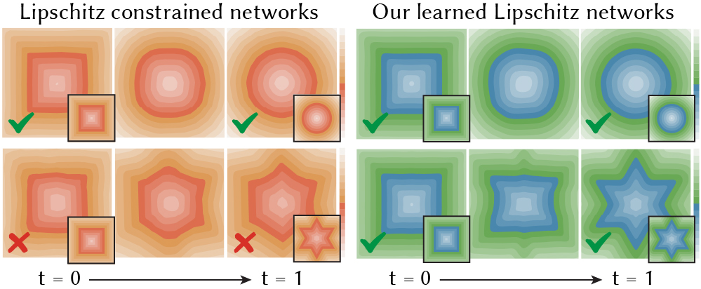
Figure 3. Different tasks require different Lipschitz constants. We manually specify the same Lipschitz constant on the top two interpolation examples. One of them is sufficient (top left) to fit the ground truth (black), but the other one is not (bottom left). In contrast, our method learns a suitable Lipschitz constant for each task (right) with the same hyperparameter.

Geometric Regularizations

Many existing approaches rely on classic measures to encourage smoothness in neural 3D mesh processing. Several methods (e.g., [Liu et al., 2019; Wang et al., 2018; Hertz et al., 2020]) use Laplacian regularization which penalizes the difference between a vertex and the center of mass of its 1-ring neighbors. Kato et al. [2018] encourage smoothness by encouraging flat dihedral angle between adjacent faces. Wang et al. [2018]; Hertz et al. [2020] penalize edge-lengths and their variance. Rakotosaona and Ovsjanikov [2020] define an isometry regularization in character deformation to obtain area preserving interpolation. Many techniques (e.g., [Chen et al., 2019]) even use a mixture of these regularizations. However, these regularizations often require the input being a manifold triangle mesh. In other representations such as neural fields, regularizations of the level set surface are difficult to be defined. Previous works also introduced other geometric regularizations for encouraging different properties, such as [Gropp et al., 2020; Williams et al., 2021]. But we exclude our discussion on those techniques because they are not directly related to the smoothness of a network function.

Network Regularizations

Given input samples, one can differentiate through a network to obtain derivative information of the network output with respect to these inputs. Then we can encourage smoothness at these input samples by penalizing the norm of the Jacobian [Drucker and Le Cun, 1991; Hoffman et al., 2019; Jakubovitz and Giryes, 2018; Varga et al., 2017; Gulrajani et al., 2017] or the Hessian [Moosavi-Dezfooli et al., 2019]. If differentiating through the network is undesirable, Elsner et al. [2021] propose to penalize the difference in the output based on the input similarity. These techniques are effective in obtaining smooth solutions at training samples, but they have no guarantee to obtain a smooth function beyond them. On the contrary, it may even promote non-smooth behavior by squeezing function changes to locations without training samples (see Fig. 2).

In lieu of this, one should use regularization techniques that do not depend on the input to a network, such as penalizing L2 norm [Tihonov, 1963] or L1 norm [Tibshirani, 1996] of the weight matrices. Other training techniques can also be used to regularize the network, such as early-stopping [Ulyanov et al., 2018; Williams et al., 2019], dropout [Srivastava et al., 2014], and learning rate decay [Li et al., 2019b]. Applying these techniques can alleviate overfitting, but how they relate to the smoothness of a network function remains an open problem. In our experiments, they produce less smooth results compared to our method (see Table 1).

Figure 4. The spectral norm regularization proposed by Yoshida and Miyato [2017] is more sensitive to the number of layers. Therefore, using the same $\alpha$ on a 5-layer and a 10-layer MLP leads to different effects (red). In contrast, our regularization (blue) leads to more consistent results.

Lipschitz Regularizations

The Lipschitz constant of neural networks has attracted huge attention because of its applications in robustness against adversarial attacks [Oberman and Calder, 2018; Li et al., 2019a], better generalization [Yoshida and Miyato, 2017], and Wasserstein generative adversarial networks [Arjovsky et al., 2017]. Several techniques have been proposed to precisely constraint the Lipschitz constant of a network. Miyato et al. [2018] normalize the weight matrices by dividing each weight matrix by its largest eigenvalue. This spectral normalization enforces a neural network to be 1-Lipschitz, a neural network with Lipschitz bound $1$, under the L2 norm. Gouk et al. [2021] rely on different weight normalization methods to constrain the Lipschitz bound under L1 and L-infinity norms. Cissé et al. [2017]; Anil et al. [2019] obtain 1-Lipschitz networks by orthonormalizing each weight matrix. Strictly constraining the Lipschitz constant of a network is not always desirable because it may lead to undesired behavior in the optimization [Gulrajani et al., 2017; Rosca et al., 2020]. In response, Terjék [2020] propose a regularization to softly encourage a network to be $c$-Lipschitz. However, these Lipschitz constrained networks often fail to achieve the prescribed Lipschitz bound because the estimated Lipschitz bound is not tight due to the ignorance of activation functions. Several papers complement this subject by proposing more accurate methods to estimate the true Lipschitz constant, such as [Virmaux and Scaman, 2018; Weng et al., 2018; Jordan and Dimakis, 2020]. Anil et al. [2019] propose a new activation function based on sorting to tighten the estimated Lipschitz bound. Unfortunately, the above-mentioned Lipschitz constrained networks require to know the target Lipschitz constant beforehand. This makes them difficult to be deployed to geometry applications because a good Lipschitz constant is unknown, thus leading to extensive hyperparameter tuning (see Fig. 3).

This inspires some Lipschitz-like regularizations, such as the spectral norm regularization which penalizes the largest eigenvalue of each weight matrix [Yoshida and Miyato, 2017]. They also show that adding regularization improves the generalizability and adversarial robustness. But this regularization does not incorporate the fact that the Lipschitz constant grows exponentially with respect to the depth of the network. In practice, it causes difficulties in hyperparameter tuning because changing the number of layers requires to also change the weight on the regularization (see Fig. 4).

3. Background in Lipschitz Networks

A neural network $f_{\theta}$ with parameter $\theta$ is called Lipschitz continuous if there exist a constant $c≥0$ such that

(1) $$\underbrace{\|f_{\theta}({\mathsf{t}}_{0})-f_{\theta}({\mathsf{t}}_{1})\|_{p}}_{\mathclap{\text{change in the output}}}≤c\ \underbrace{\|{\mathsf{t}}_{0}-{\mathsf{t}}_{1}\|_{p}}_{\mathclap{\text{change in the input}}}$$

for all possible inputs ${\mathsf{t}}_{0},{\mathsf{t}}_{1}$ under a $p$-norm of choice. The parameter $c$ is called the Lipschitz constant. Intuitively, this constant $c$ bounds how fast this function $f_{\theta}$ can change.

As pointed out by several previous papers mentioned in Sec. 2, the Lipschitz bound $c$ of an fully-connected network with 1-Lipschitz activation functions (e.g., ReLU) can be estimated via

(2) $$c=∏_{i=1}^{L}\|{\mathsf{W}}_{i}\|_{p},$$

where ${\mathsf{W}}_{i}$ is the weight matrix at layer $i$ and $L$ denotes the number of layers. This estimate is a loose upper bound due to the ignorance of activation functions, but in practice, optimizing this upper bound is still effective (i.e. [Miyato et al., 2018]).

In the past years, different ways of controlling the Lipschitz bound of a network have been studied. A dominant strategy is to perform weight normalization. For instance, if one wants to enforce the network to be 1-Lipschitz $c=1$, then one can achieve this by normalizing the weight such that $\|{\mathsf{W}}_{i}\|_{p}=1$ after each gradient step during training. The normalization scheme depends on the choice of different matrix $p$-norms:

(3) $$\|{\mathsf{M}}\|_{2}=\sigma_{\text{max}}({\mathsf{M}}),$$

(4) $$\|{\mathsf{M}}\|_{1}=\max_{j}∑_{i}|m_{ij}|,\quad\|{\mathsf{M}}\|_{∞}=\max_{i}∑_{j}|m_{ij}|,$$

where $\sigma_{\text{max}}({\mathsf{M}})$ denotes the maximum eigenvalue of ${\mathsf{M}}$. Thus, when $p=2$, weight normalization consists of rescaling the weight matrix based on its maximum eigenvalue. Popular techniques include spectral normalization based on the power iteration [Miyato et al., 2018] and the Björck Orthonormalization [Björck and Bowie, 1971; Anil et al., 2019]. When $p=\infty$ ($p=1$), weights normalization is simply scaling individual rows (columns) to have a maximum absolute row (column) sum smaller than a prescribed bound.

These matrix norms are also related to each other. Let ${\mathsf{M}}$ be a matrix with size $m$-by-$n$, its $2$-norm is bounded by its $1$-norm and $\infty$-norm in the following relationships

(5) $$\frac{1}{\sqrt{n}}\|{\mathsf{M}}\|_{\infty}≤\|{\mathsf{M}}\|_{2}≤\sqrt{m}\|{\mathsf{M}}\|_{\infty}$$

(6) $$\frac{1}{\sqrt{m}}\|{\mathsf{M}}\|_{1}≤\|{\mathsf{M}}\|_{2}≤\sqrt{n}\|{\mathsf{M}}\|_{1}.$$

This implies that optimizing the Lipschitz bound under a particular choice of norms will effectively optimize the bound measured by the other norms. One could also consider the entry-wise matrix norm $\|{\mathsf{M}}\|_{p,q}$ (see [Horn and Johnson, 2012]). But we leave the exploration of the most effective strategy as future work.

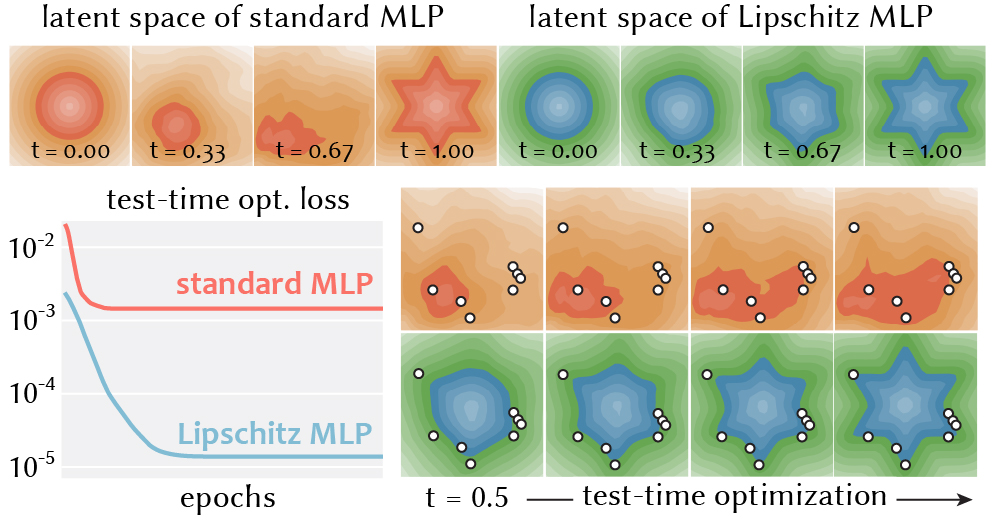
Figure 5. We demonstrate the importance of smooth latent space on a toy test-time reconstruction of a 2D point cloud. We train a standard MLP and our Lipschitz MLP to interpolate a circle ($t=0$) to a star ($t=1$). Then we sample points on the zero-isoline of the star (white points) and optimize the latent code to fit those points (with initial ${\mathsf{t}}=0.5$). Our smooth latent space enables latent optimization to find the correct solution (bottom blue) while the non-smooth one suffers from poor local minimum (bottom red).

4. Method

Throughout we use $f_{\theta}({\mathsf{x}},{\mathsf{t}})$ to denote the forward model of an implicit shape parameterized by a neural network, namely a mapping from a tuple of a location ${\mathsf{x}}∈\mathbb{R}^{d}$ in $d$-dimensional space and a latent code ${\mathsf{t}}∈\mathbb{R}^{|{\mathsf{t}}|}$ to $\mathbb{R}$. $f_{\theta}$ has parameters $θ=\{{\mathsf{W}}_{i},{\mathsf{b}}_{i}\}$ containing weights ${\mathsf{W}}_{i}$ and biases ${\mathsf{b}}_{i}$ of each layer $i$.

Our goal is to train a neural network that is smooth with respect to its latent code ${\mathsf{t}}$. This property is important for shape editing and in applications requiring a well-structured latent space in which a small change in ${\mathsf{t}}$ results in a small change to the output (see Fig. 5).

A straightforward idea is to augment the loss function with some smoothness regularizations, such as the Dirichlet energy. Specifically, one would draw a bunch of samples points ${\mathsf{t}}_{j}$ in the latent space and turn the original loss function $\mathcal{L}$ into

(7) $$\mathcal{J}(\theta)=\mathcal{L}(\theta)+\alpha\ \sum_{j}\|\frac{∂f_{\theta}}{∂{\mathsf{t}}}({\mathsf{x}},{\mathsf{t}}_{j})\|^{2}.$$

Although being effective in encouraging a smooth neural field $f_{\theta}$ with respect to the change in latent code at the sampled locations ${\mathsf{t}}_{j}$, it often results in non-smooth behavior elsewhere. For instance, in Fig. 2, we apply the Dirichlet regularization to a toy task: interpolating between two neural SDFs conditioned on two latent codes, ${\mathsf{t}}=0$ and ${\mathsf{t}}=1$, with 1D latent dimension. In this example, we minimize the Dirichlet energy at ${\mathsf{t}}=\nicefrac{{1}}{{3}},\nicefrac{{2}}{{3}}$. The network is able to find a perfectly smooth (constant) solution at the sampled ${\mathsf{t}}$s, but it squeezes all the changes at the very beginning and results in non-smooth behavior $0<{\mathsf{t}}<\nicefrac{{1}}{{3}}$. This issue is even more troublesome when the latent dimension is large and sampling densely is intractable. A more desirable approach is to guarantee smoothness for all possible latent inputs without the need to densely sample the latent space.

Our main idea is to define the smoothness energy solely based on network parameters (i.e. weights of a neural network) regardless of the inputs. One promising solution is to encourage Lipschitz continuity with respect to the inputs, in our case the latent code ${\mathsf{t}}$, and use its Lipschitz constant $c$ as a proxy for smoothness. Specifically, we want the network to satisfy

(8) $$\|f_{\theta}({\mathsf{x}},{\mathsf{t}}_{0})-f_{\theta}({\mathsf{x}},{\mathsf{t}}_{1})\|_{p}≤c\ \|{\mathsf{t}}_{0}-{\mathsf{t}}_{1}\|_{p}$$

for all possible combinations of ${\mathsf{x}},{\mathsf{t}}_{0},{\mathsf{t}}_{1}$. As the upper bound of the Lipschitz constant $c=∏_{i}\|{\mathsf{W}}_{i}\|_{p}$ only depends on the weight matrices ${\mathsf{W}}_{i}$, $c$ is independent to the choice of inputs. Therefore, by decreasing $c$, one guarantees smoothness everywhere even beyond the training set (see Fig. 1).

To decrease the Lipschitz constant and encourage smoothness, we present a new regularization. The key idea is to treat the Lipschitz constant of a network as a learnable parameter and minimize it, instead of a pre-determined value (e.g., [Miyato et al., 2018]). There are many possible ways one can formulate such a regularization and there is not a single formulation that is uniformly the best. We first present our recommended solution and defer the comparison with alternative formulations in Sec. 4.2.

4.1. Lipschitz Multilayer Perceptron

The first question is to choose a $p$-norm to measure the Lipschitz constant Eq. (8). In our case, we have no restriction on the choice of $p$-norm. We solely want to have a small Lipschitz constant to encourage smooth behavior with respect to the change of the latent code ${\mathsf{t}}$. Thus, we simply choose the matrix $\infty$-norm due to its efficiency (see the inset). But if applications require other choices, our approach is also applicable.

After determining the matrix norm, our method only requires two simple modifications to a standard fully-connected network: adding a weight normalization to each fully connected layer, parameterized by a learnable Lipschitz variable, and a regularization term to encourage an overall small Lipschitz constant that is minimized together with the task loss function.

4.1.1. Weight Normalization Layer

Our weight normalization shares the same spirit as the other weight normalization methods for accelerating training [Salimans and Kingma, 2016] and generalization ability [Huang et al., 2018]. But the key difference is that our normalization is based on the Lipschitz constant of a layer, which is more suitable for obtaining a smooth network.

We augment each layer of an MLP ${\mathsf{y}}=σ({\mathsf{W}}_{i}{\mathsf{x}}+{\mathsf{b}}_{i})$ with a Lipschitz weight normalization layer given a trainable Lipschitz bound $c_{i}$ for layer $i$

(9) $${\mathsf{y}}=σ(\widehat{\mathsf{W}}_{i}{\mathsf{x}}+{\mathsf{b}}_{i}),\quad\widehat{\mathsf{W}}_{i}=\textit{normalization}\,({\mathsf{W}}_{i},\textit{softplus}\,(c_{i})),$$

where the $\textit{softplus}\,(c_{i})=\ln(1+e^{c_{i}})$ is a reparameterization designed to avoid infeasible negative Lipschitz bounds. In most of our cases $c_{i}≈\textit{softplus}\,(c_{i})$ because $c_{i}$ is often a large positive number. Due to our choice of using $\infty$-norm, this normalization is efficient and simple: we scale each row of ${\mathsf{W}}_{i}$ to have the absolute value row-sum less than or equal to $\textit{softplus}\,(c_{i})$. If one of the rows already has the absolute value row-sum smaller than $\textit{softplus}\,(c_{i})$, then no scaling is performed. With this normalization layer, even if the raw weight matrix ${\mathsf{W}}_{i}$ has a Lipschitz constant greater than $\textit{softplus}\,(c_{i})$, this normalization can still guarantee the Lipschitz constant is bounded by $\textit{softplus}\,(c_{i})$. Therefore, we never clip the weights during training.

Implementation

Our method can be implemented in a few lines of code. Given the weight matrix Wi and the per-layer Lipschitz upper bound ci, the normalization layer can be implemented in JAX [Bradbury et al., 2018] as

⬇

import jax.numpy as jnp

def normalization(Wi, softplus_ci): # L-inf norm

absrowsum = jnp.sum(jnp.abs(Wi), axis=1)

scale = jnp.minimum(1.0, softplus_ci/absrowsum)

return Wi * scale[:,None]

and each layer of the Lipscthiz MLP is simply

⬇

y = sigma(normalization(Wi, softplus(ci))*x + bi)

where sigma denotes the activation function and softplus is the built-in softplus function in JAX.

Although being efficient, using our Lipschitz weight normalization will still increase the training time. For example, in the 2D interpolation task (such as Fig. 3), adding our normalization slows down the training from 265.83 epochs per second down to 229.95 epochs per second.

However, incorporating our regularization will not influence the performance during test time because one can explicitly construct the normalized weight matrix $\widehat{{\mathsf{W}}}_{i}$ by clipping the weight matrix ${\mathsf{W}}_{i}$ with the learned constant $c_{i}$. Then, one can use the vanilla MLP with the normalized weights $\widehat{{\mathsf{W}}}_{i}$ as their final model.

4.1.2. Our Lipschitz Regularization

The second ingredient is to augment the original loss function $\mathcal{L}$ with a Lipschitz regularization. Our Lipschitz regularization is defined simply as the Lipschitz bound of the network. But instead of directly defining on the weight matrices, we define it on the parameterized per-layer Lipschitz bounds $\textit{softplus}\,(c_{i})$ in the normalization layer Eq. (9). Specifically, we augment the original loss function $\mathcal{L}$ with a Lipschitz term as

(10) $$\boxed{\mathcal{J}(\theta,C)=\mathcal{L}(\theta)+\alpha∏_{i=1}^{l}\textit{softplus}\,(c_{i})}$$

where we use $C=\{c_{i}\}$ to denote the collection of per-layer Lipschitz constants $c_{i}$ used in the weight normalization. As mentioned in Eq. (2), the product of per-layer Lipschitz constants is the Lipschitz bound of the network.

4.2. Comparison with Alternatives

There are many ways one can implement and formulate a Lipschitz regularization. In this section, we compare our formulation with alternative formulations. As the amount of regularization $\alpha$ will influence the analysis, we perform parameter sweeping for each formulation independently and compare their best set-ups.

Figure 6. Our method converges to a smoother result compared to the $k$-Lipschitz architecture described in [Anil et al., 2019] (see Eq. (11)). We use the same $\alpha$ for both networks because we both define the regularization as the raw Lipschitz constant of the network.

One solution is to design a regularization based on the architecture of the $k$-Lipschitz networks, such as the one suggested by Anil et al. [2019]. Specifically, Anil et al. [2019] constrain all the layers to be $1$-Lipschitz and multiply the final layer with a constant $k$ to make it $k$-Lipschitz. A possible formulation to make it learnable is to simply treat the $k$ as the Lipschitz regularization term

(11) $$\mathcal{J}(\theta,k)=\mathcal{L}(\theta)+\alpha k$$

However, we struggle to use this formulation in Eq. (11) to find a good local minimum even for the simple 2D interpolation task (see Fig. 6). Moreover, when one switches to other types of activations, the result is even worse because the distributive property of per-layer scaling no longer holds.

Another alternative is the formulation by Yoshida and Miyato [2017] which defines a Lipschitz-like regularization as the summation of squared Lipschitz bounds of each layer. Generalizing the definition in [Yoshida and Miyato, 2017] to $p$-norms gives us

(12) $$\mathcal{J}(\theta)=\mathcal{L}(\theta)+\alpha∑_{i=1}^{l}\|{\mathsf{W}}_{i}\|_{p}^{2}$$

Although this formulation can effectively find a smooth solution given a good $\alpha$, finding a good $\alpha$ is not easy with this formulation. This formulation fails to capture the exponential growth of the Lipschitz constant with respect to the network depth (see Eq. (2)). In practice, it implies that the formulation Eq. (12) proposed by Yoshida and Miyato [2017] requires a different $\alpha$ when we change the depth of the network. In Fig. 4, we use the spectral norm for the method by Yoshida and Miyato [2017] and show that the same $\alpha$ results in different behavior for networks with different capacities. In contrast, our method leads to a more consistent behavior with the same $\alpha$.

Another alternative is to define the Lipschitz regularization directly on the weight matrices, without the normalization layer.

(13) $$\mathcal{J}(\theta)=\mathcal{L}(\theta)+\alpha∏_{i=1}^{l}\|{\mathsf{W}}_{i}\|_{\infty}$$

This approach works equally well as our method on narrower networks, but it converges slower on wider ones. We suspect that this is because the $\infty$-norm only depends on a single row of the weight matrix. So on a wider network, this formulation requires more epochs to penalize its parameters. In the inset, we show the convergence of a 2-layer MLP with 1024 neurons each layer on 2D interpolation.

Another tempting solution is to consider the log of the Lipschitz bound to turn the product in Eq. (10) into a summation

(14) $$\mathcal{J}(\theta,C)=\mathcal{L}(\theta)+\alpha\sum_{i=1}^{l}\log(\textit{softplus}\,(c_{i}))$$

However, this makes the regularization unbounded because log goes to negative infinity when one of the Lipschitz constants approaches zero. In practice, this implies the tendency to continue penalizing the layer with a smaller Lipschitz constant. In a few cases, we did not observe the Lipschitz constants to converge. In the inset, we visualize the per-layer Lipschitz constants of a network trained on the ShapeNet [Chang et al., 2015], where the layers are ordered in rainbow colors. We can observe that one of the Lipschitz constants continues to decrease (purple) even after a week of training.

Figure 7. Our Lipschitz regularization is applicable to different implicit representations. We fit an occupancy network [Mescheder et al., 2019a] to two shapes (green) at $t=0$ and $t=1$ with (blue) and without (red) our Lipschitz regularization. Our method generates smoother interpolation/extrapolation results.

Table 1. We compute the squared norm of the Jacobian matrix ${\mathsf{J}}$ via back-propagation. We report the average and the maximum value of the $\|{\mathsf{J}}\|^{2}$ for all training data and show that our Lipschitz regularization achieves a smoother solution compared to other weight decay methods.

Metrics	Ours	L2	L1	Vanilla
mean $\|{\mathsf{J}}\|^{2}$	1.009	1.020	1.016	1.021
max $\|{\mathsf{J}}\|^{2}$	9.419	21.181	17.361	23.658

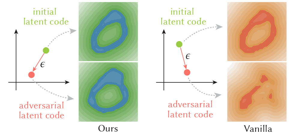
Figure 8. We perform a (virtual) adversarial attack which perturbs the latent code with the fast gradient sign method [Goodfellow et al., 2015]. Vanilla AE is vulnerable to the attack so the SDF of “0” is completely destroyed. In contrast, our Lipschitz regularized network is more robust to the attack.

4.3. Comparison with Weight Decay

Our Lipschitz regularization can be perceived as a variant of the weight decay regularization, such as the Tikhonov (L2) regularization [Tihonov, 1963] and Lasso (L1) [Tibshirani, 1996]. These weight decay methods are often used to avoid overfitting and improve generalization ability. However, it is unclear what their relationships are with respect to the smoothness of the network. As a result,

networks trained using weight decay are less smooth (measured by Lipschitz constant) compared to the network trained with our Lipschitz regularization (see the inset).

Our Lipschitz regularization also leads to a smoother network compared to other weight decay measured by a popular metric, square Jacobian norm. To verify this, we train autoencoders (AE) to reconstruct the MNIST digits represented as signed distance functions. In Table 1, our Lipschitz AE leads to smaller Jacobian norms compared to the vanilla AE, the L1 regularized AE, and the L2 regularized AE. We provide experimental details in App. A.6.

Besides weight decay, there are other types of regularization that are not defined on network weights, such as adding noise [Poole et al., 2014] and Dropout [Srivastava et al., 2014]. These methods can complement our approach, such as [Gouk et al., 2021]. We leave the study on mixing and matching these regularizations as future work. For a more comprehensive discussion, please refer to a survey on regularization [Moradi et al., 2020].

Figure 9. Our method only encourages smooth interpolation. Thus our method cannot extract high-level information, such as semantics, from only a handful of shapes. Therefore, when we interpolate between animal shapes (green), the interpolated results (blue) may not be realistic animals.

5. Experiments

Our regularization encourages a fully connected network to output Lipschitz continuous functions and is therefore applicable to different tasks that favor smooth solutions. In this section, we examine at the effectiveness of our approach in improving the robustness of a network, shape interpolation, and test-time optimization.

5.1. Adversarial Robustness

Adversarial attacks are small, structured changes made to a network’s input signal that cause a significant change in output [Szegedy et al., 2014]. As been previously shown, Lipschitz continuous networks can improve robustness against adversarial attacks [Li et al., 2019a]. Here we demonstrate that our proposed regularization can serve that purpose. To that end we train an AE to reconstruct the signed distance functions of MNIST digits from their input image. We then adversarially perturb the latent code as described in Fig. 8, and show that Lipschitz MLP is more robust to adversarial perturbations than a standard one. We quantitatively evaluate the robustness against this type of latent adversarial attack on all the MNIST digits. A standard AE results in an average $0.06$ and maximum $0.34$ difference in the signed distance value. In contrast, our Lipschitz AE is more robust with only an average $0.03$ and maximum $0.16$ difference. We refer readers to App. A.6 for details about this experiment.

5.2. Few-Shot Shape Interpolation & Extrapolation

Shape interpolation is a fundamental task and several classic methods exist, such as [Solomon et al., 2015] and [Kilian et al., 2007]. When shapes are mapped from a latent descriptor to 3D via a decoder, interpolation through latent space traversal often requires training on abundant data so that the latent space is well structured. Our regularization can aid shape interpolation and extrapolation in given only sparse training shapes. In Fig. 13, we provide several 3D SDF interpolation examples trained on only two shapes. Our method is also applicable to other implicit representations. In Fig. 7, we evaluate our method to interpolate the occupancy [Mescheder et al., 2019a] which assigns each point in $\mathbb{R}^{3}$ a binary value $[0,1]$ representing whether it is inside or outside.

Figure 10. Our method enables smooth interpolation between few training shapes. By training our model on three examples (green), we can generate high-quality novel shapes by interpolating latent codes of training shapes.

5.3. Reconstruction with Test Time Optimization

Autoencoders are popular in reconstructing the full shape from a partial point cloud. However, simply forward passing the partial points through the AE often outputs unsatisfying results. A common way to resolve this issue is to further optimize the latent code of the partial point cloud during test time [Gurumurthy and Agrawal, 2019]. Despite being effective, test time optimization is very sensitive to parameters in the optimization (e.g., initialization) and suffers from bad local minima. Duggal et al. [2022] even propose a dedicated method aiming for resolving this issue of test-time optimization.

We discover that our Lipschitz regularization can complement the research in stabilizing test time optimization. Simply by adding our Lipschitz regularization to the vanilla autoencoder set-up, we can encourage a smoother latent manifold and stabilize the test time optimization. In Fig. 11 and Table 2, we show that we achieve a better reconstruction result both qualitatively and quantitatively. Our method can complement the method based on training additional networks, such as adding a discriminator [Duggal et al., 2022] or a generative adversarial network [Gurumurthy and Agrawal, 2019]. But we leave them as future work.

Figure 11. Encouraging smoothness with respect to the change in latent code encourages the latent space to be more compact. In the application of test time optimization, our method yields a better reconstruction (blue) given partial observations (left).

Table 2. We quantitatively evaluate the test time optimization. Given a ground truth point cloud from the test set, we delete the right-half of the point to obtain a partial point cloud and then we perform test-time optimization to reconstruct the full shape back. We report the Chamfer distance and Hausdorff distance between the ground truth point cloud and our reconstructed full shape averaged across the test set.

Metrics	Lipschitz DeepSDF	DeepSDF
average Chamfer distance	0.0013	0.0343
average Hausdorff distance	0.1270	0.3441

6. Conclusion & Future Work

Our regularization encourages fully connected networks to have a small Lipschitz constant. Our regularization is defined on a loose upper bound of the true Lipschitz constant. Using a tighter estimate would benefit applications that require more precise control. Our shape interpolation behaves similarly to linear interpolation. Incorporating the Wasserstein metric into our smoothness measure could encourage shape interpolation to behave more like optimal transport. Furthermore, encouraging learning high-level structural information from few examples would aid to the experiment on few shot shape interpolation (see Fig. 9). Our Lipschitz regularization is a generic technique to encourage smooth neural network solutions. However, our experiments are mainly conducted on neural implicit geometry tasks. We would be interested in applying our regularization to other tasks beyond geometry processing.

Appendix A Experimental & Implementation Details

For all our experiments, we initialize the per-layer Lipschitz constant $c_{i}=\|{\mathsf{W}}_{i}\|_{\infty}$ in Eq. (10) as the Lipschitz constant of the initial weight matrix. The weight matrices are initialized with the method by [Glorot and Bengio, 2010] if the activation is $\tanh$ and with the method by He et al. [2015] if the activation is ReLU or its variants. In the following subsections, we present details of individual experiments in the main text.

A.1. 3D Neural Implicit Interpolation

We use the DeepSDF architecture [Park et al., 2019] to design the interpolation experiment of 3D neural SDFs (Fig. 1, 10, 9). The inputs to our network are the query location in $\mathbb{R}^{3}$ and the latent code $t$. Our network consists of 5 hidden layers of 256 neurons with the $\tanh$ activation. We multiply the input point $x$ with one hundred $100x$ to avoid the possibility that the network smoothness in the latent code is bounded by spatial smoothness. The last layer is a linear layer outputting the signed distance value at the input query location. The training shapes are normalized to the bounding box between 0 and 1. We use the mean square error (MSE) as our loss function $\mathcal{L}(\theta)$ for our baseline model. We augment the MSE loss with our Lipschitz regularization Eq. (10) (with $α=10^{-6}$) to evaluate the influence of our method. We compute the MSE loss by sampling $10^{5}$ points where $40\%$ of them are on the surface, $40\%$ are near the surface, and $20\%$ are drawn from uniformly sampling the bounding box. We use the Adam optimizer [Kingma and Ba, 2015] with its default parameters presented and learning rate $10^{-4}$.

For our experiment on occupancy interpolation [Mescheder et al., 2019b] (Fig. 7), we use the same architecture as our SDF experiments and append a sigmoid function right before the output. Our loss function is the cross-entropy loss with and without our Lipschitz regularization (with $α=10^{-6}$).

In these interpolation experiments, we pre-determine the latent codes for each shape we want to interpolate. For example Fig. 1, we minimize the loss with respect to the SDF of a torus when $t=0$ and with the double torus when $t=1$. Similarly, we also use $t=0,1$ in our occupancy interpolation Fig. 7. In Fig. 10, the three sets of code for the green shapes are [0,0], [1,0], [0.5, 0.866]. In Fig. 9, the latent code for the four shapes are set to be one-hot vectors, such as [1,0,0,0].

A.2. 2D Neural Implicit Interpolation

The experiments on interpolating 2D neural implicits are similar to the above-mentioned 3D interpolation ones App. A.1. We minimize the MSE loss with Adam and use the DeepSDF architecture. The only difference is that the network is smaller and our training data is sampled uniformly on the 2D space. In Fig. 2, 3, we use a MLP with 5 hidden layers of 64 neurons with ReLU activation. Specifically, we set the Dirichlet regularization Eq. (7) to be $10^{-4}$ in Fig. 2. We manually set the Lipschitz constant per layer to be $1.4$ in Fig. 3. For our Lipschitz regularization, we set $α=3×10^{-6}$.

A.3. Toy 2D test time optimization

In Fig. 5, we present a toy test time optimization to demonstrate the importance of having a smooth latent space. We use the same training set-up as App. A.2 to train our interpolation networks. During test-time, we initialize the latent code to be $t=0.5$ and we randomly sample 8 points on the iso-line of the star shape and minimize the square distance at these sample points. Intuitively, if the loss is minimized, these points will lie on the zero iso-line of the optimized SDF. In Fig. 5, we show the optimization using Adam. We also tried to optimize the code using SGD, but we only notice a small difference in this toy set-up.

Figure 12. In this simple toy example, test-time optimization using SGD gives us similar result compared to the one optimized with Adam (see Fig. 5).

Figure 13. We fit neural networks to the signed distance field of a shape when the latent code $t=0$ and another shape when $t=1$ (green). Our Lipschitz regularization encourages smooth interpolation and extrapolation (blue) even when trained on only a pair of shapes.

A.4. Test time optimization

We evaluate test time optimization on the chair category of the ShapeNet dataset [Chang et al., 2015], which contains 4746 shapes. Our network architecture follows the baseline autoencoder model in [Duggal et al., 2022]. The encoder is a PointNet [Qi et al., 2017]. Specifically, the input to our PointNet is a point location ${\mathsf{p}}_{i}$ in $\mathbb{R}^{3}$. We pass this point ${\mathsf{p}}_{i}$ to a fully-connected network of size [3, 256, 512] with $\tanh$ activation to transform this point to a feature vector ${\mathsf{z}}_{i}$ of size 512. This fully-connected network is used to independently process each point ${\mathsf{p}}_{i}$ in the point cloud. Thus, after this step, we obtain a $n$-by-512 feature matrix where $n$ is the number of points. We perform a max-pooling for this feature matrix to obtain a feature vector ${\mathsf{z}}_{\text{global}}$ of size 512, encoding the global information of the point cloud. We then concatenate this global feature vector ${\mathsf{z}}_{\text{global}}$ is with the feature vector of individual point feature ${\mathsf{z}}_{i}$. After concatenation, we pass this local-global feature [${\mathsf{z}}_{i}$, ${\mathsf{z}}_{\text{global}}$] to the second fully-connected network of size [1024, 512, 256] with $\tanh$ activation. Similar to the previous step, we use this shared network to process each point independently. Thus, after processing all the points, we will obtain a $n$-by-256 feature matrix. We then perform another max-pooling to turn this $n$-by-256 feature matrix into a 256 global feature vector. To prevent the latent codes from diverging to an arbitrarily vector with large magnitude, apply a sigmoid function to the global feature vector ensure each latent code lies between 0 and 1. We then treat this as the final feature representation of the point cloud after the encoding process.

After the encoding process, our decoder is a DeepSDF [Park et al., 2019] which takes the query location in $\mathbb{R}^{3}$ and the 256 latent vector from the encoder as its input, and then outputs the signed distance value. The decoder has size [259, 1024, 1024, 1024, 512, 256, 128, 1] with the leaky ReLU activation. Similar to App. A.1, we minimize the MSE loss with Adam and set the learning rate to be $10^{-4}$. To evaluate our method, we add a Lipschitz regularization with $α=10^{-11}$ to the decoder during training (see Fig. 11).

For the test time optimization, given a partial point cloud, we initialize the latent code by passing through our PointNet encoder. With this code, we pass each point in the point cloud to the decoder and minimize the square SDF value. Intuitively, we want the point on the partial point cloud to lie on the zero iso-surface. In addition, we also augment an Eikonal term [Gropp et al., 2020] weighted by $1e-2$ to encourage the output to be an SDF-like function. We minimize this loss (square SDF and an Eikonal loss) by changing the latent code parameter (the parameter before applying the sigmoid) during test time with Adam with a learning rate $10^{-4}$ until converged.

A.5. Alternative Lipschitz Regularizations

We evaluate our method against the method proposed in [Anil et al., 2019] (Eq. (11)) and another alternative mentioned in Eq. (13) on 2D interpolation tasks App. A.2. We use a 5 layer ReLU MLP with 64 neurons on each hidden layer. Because these approaches are all defined on the Lipschitz bound of the network, we use the same $α=10^{-6}$ for a fair comparison.

We also compare against the method by Yoshida and Miyato [2017] on 2D interpolation. We use 5 and 10 layers ReLU MLP with 64 neurons on each hidden layer respectively. We use $α=10^{-5}$ for the method by Yoshida and Miyato [2017] and $α=10^{-6}$ for our regularization.

In Eq. (14), we evaluate it on a large network trained on the ShapeNet [Chang et al., 2015]. We notice that if the task is simple, such as 2D interpolation, whether to take a log result in similar performance when we have a good $α$. But when evaluating on large experiments with large networks, minimizing the log of the Lipschitz bound Eq. (14) may start to have issues on convergence. In this experiment specifically, we use the same training set-up as App. A.4 and we use $α=10^{-6}$.

Figure 14. We perform adversarial attacks in the latent space, the same setup as Fig. 8. We can observe that Vanilla AE is vulnerable to the attack so the initial SDFs (first row) are completely destroyed after adversarial perturbations (second row). In contrast, our Lipschitz regularized network is more robust to the attack (third and the fourth rows).

A.6. MNIST Implicit Autoencoder

The experiments presented in Sec. 4.3 and Sec. 5.1 are evaluated on the MNIST dataset (60000 hand-written digits) represented in 28-by-28 SDF images. Our autoencoder uses two MLPs as our encoder and decoder. Our encoder has size [784, 256, 128, 64, 32] with leaky ReLU activation. It takes the image of an MNIST digit (in SDF form) as the input and outputs a latent code with dimension 32. Similar to App. A.4, we then apply a sigmoid function on the output to ensure the actual latent code lies between 0 and 1. The inputs to our decoder are the latent code and the position in the image space. It outputs the SDF value at the location. Our decoder has dimension [35, 128, 128, 128, 1] with the sorting activation [Anil et al., 2019]. We multiply the input position by 100 to avoid the possibility that the network is constrained by spatial smoothness We use Adam with a learning rate $10^{-4}$ to minimize the MSE loss evaluated on the 28-by-28 regular 2D grid. For each regularization (L1, L2, and ours), we perform parameter sweeping on log scale and report the best one in terms of test accuracy. Specifically, we use $10^{-7}$ for both the L1 and L2 regularization, and $10^{-6}$ for our Lipschitz regularization.

To construct an adversarial perturbation in the latent space, we fist obtain the initial latent code ${\mathsf{t}}_{i}$ of a valid MNIST digit by passing an image ${\mathsf{I}}_{i}$ from the training/testing set to our encoder, then we follow the fast gradient signed method proposed in [Goodfellow et al., 2015] to compute the adversarial perturbation. Specifically, we set the loss function $\mathcal{J}$ to be squared L2 pixel difference between the input MNIST digit ${\mathsf{I}}_{i}$ and the decoded image output by the network $f_{θ}({\mathsf{t}})$ using another code ${\mathsf{t}}$. Then the adversarial latent code is constructed by

(15) $${\mathsf{t}}_{\text{adv.}}={\mathsf{t}}_{i}+ϵ\ \text{sign}\Big{(}\frac{∂\mathcal{J}({\mathsf{I}}_{i},f_{θ}({\mathsf{t}}))}{∂{\mathsf{t}}}\Big{)}$$

with predetermined small magnitude $ϵ=0.05$. Then the adversarial MNIST digits can be obtained by visualizing the output of the network with the adversarial code $f_{\theta}({\mathsf{t}}_{\text{adv.}})$.

Appendix B Relationship with Weight Normalization

Weight Normalization is a reparameterization technique proposed by Salimans and Kingma [2016] to accelerate the training process. The key idea is to parameterize the weight matrix ${\mathsf{W}}$ with a trainable matrix ${\mathsf{V}}$ and a trainable scaling factor $g$

(16) $${\mathsf{W}}=g×\frac{{\mathsf{V}}}{\|{\mathsf{V}}\|}$$

where the matrix ${\mathsf{V}}$ is normalized to have unit norm and $g$ is the scaling factor that controls the magnitude of ${\mathsf{W}}$. This reparameterization is similar to our weight normalization layer in Sec. 4.1.1, but with a different norm. However, the key difference is that this reparameterization along is insufficient to guarantee smoothness. In the first row of Fig. 15, we can observe that solely with the method by Salimans and Kingma [2016] still results in non-smooth interpolation. This is because there is no regularization to encourage small $g$. In the second row of Fig. 15, we demonstrate the flexibility of our method that we can apply our Lipschitz regularization to encourage small $g$ under the reparameterization in [Salimans and Kingma, 2016] and successfully lead to smooth interpolation results.

Figure 15. Our Lipschitz regularization can complement other reparameterization schemes, such as the weight normalization by Salimans and Kingma [2016]. We show that solely with weight normalization is insufficent for obtain smooth results (top row), but our method can be used jointly with [Salimans and Kingma, 2016] to obtain smooth interpolation (bottom row).

Appendix C Comparison with Spectral Normalization

Spectral Normalization proposed by Miyato et al. [2018] is a method to constrain the Lipschitz bound of a network. As discussed in Sec. 2, these Lipschitz constrained networks are sensitive to the choice of the Lipschitz bound. In most geometry applications, a good choice of bound is unknown, thus it requires extensive hyperparameter tuning. In Fig. 16, we show that the results of Lipschitz constrained networks change dramatically when increasing the bounds. Our method, instead, results in smoother change with better results when playing with our regularization parameter $\alpha$.

Figure 16. Lipschitz constrained networks, such as [Miyato et al., 2018], are sensitive to the change of the prescribed Lipschitz bound. We can observe a dramatic change from too smooth (1st row) to too non-smooth (3rd row) with a minor logarithmic scaling of the initial Lipschitz bound $c$. In contrast, our method (blue) is more robust with respect to the change of our regularization weight $\alpha$.