A Data-Augmentation Is Worth A Thousand Samples:
Exact Quantification From Analytical Augmented Sample Moments

Abstract

Data-Augmentation (DA) is known to improve performance across tasks and datasets. We propose a method to theoretically analyze the effect of DA and study questions such as: how many augmented samples are needed to correctly estimate the information encoded by that DA? How does the augmentation policy impact the final parameters of a model? We derive several quantities in close-form, such as the expectation and variance of an image, loss, and model’s output under a given DA distribution. Those derivations open new avenues to quantify the benefits and limitations of DA. For example, we show that common DAs require tens of thousands of samples for the loss at hand to be correctly estimated and for the model training to converge. We show that for a training loss to be stable under DA sampling, the model’s saliency map (gradient of the loss with respect to the model’s input) must align with the smallest eigenvector of the sample variance under the considered DA augmentation, hinting at a possible explanation on why models tend to shift their focus from edges to textures.

1 Introduction

Data augmentation is a prevalent technique in training deep learning models. These models $f_{\theta}$, governed by some parameters $\theta\in\Theta$, are trained on the train set and expected to generalize to unseen samples (test set). Data Augmentation (DA) serves to improve this generalization behavior of the models. Assuming that the space $\mathcal{F}\triangleq\{f_{\theta}:\forall\theta\in\Theta\}$ is diverse enough, theoretically, an accurate DA policy is all that is needed to close any performance gap between the train and test sets (Unser, 2019; Zhang et al., 2021).

Figure 1: We propose a novel way to express Data Augmentation (DA) analytically that allows us to understand the impact of DA on the learned parameters of a model and quantify DA’s sample efficiency. We model the transformation of an image through a matrix-vector multiplication of the flattened image (red) and a sparse matrix (blue) representing the transform. This allows us to compute the analytical expectation and variance of the transformed data (or any function computed with it) in closed form with respect to the transformation parameters.

While there are multiple ways to maximize test set performance in a finite data regime, such as restricting the space of models $\mathcal{F}$, adding regularization on $f_{\theta}$ etc., DA continues to play a critical role for good performance (Perez & Wang, 2017; Taqi et al., 2018; Shorten & Khoshgoftaar, 2019). Some regimes such as self-supervised learning (SSL), rely entirely on augmentations (Misra & Maaten, 2020; Zbontar et al., 2021). Despite its empirical effectiveness, our understanding of DA has many open questions, three of which we propose to study: (a) how do different DAs impact the model’s parameters during training?; (b) how sample-efficient is the DA sampling, i.e., how many DA samples a model must observe to converge?; and (c) how sensitive is a loss/model to the DA sampling and how this variance evolves during training as a function of the model’s ability to minimize the loss at hand, and as a function of the model’s parameters?

Our goal is to analytically derive some preliminary answers and insights into those three areas enabled by a novel image transformation operator that we introduce in Section 3.2 coined Data-Space Transform (DST). We summarize our contributions below:

1. we derive the analytical first order moments of augmented samples, and of the losses employing augmented samples (Section 3.3), effectively providing us with the explicit regularizer induced by each DA (Section 3.4)

2. we quantify the number of DA samples that are required for a model/loss to obtain a correct estimate of the information conveyed by that DA (Section 4.1)

3. we derive the sensitivity, i.e. variance, of a given loss and model under a DA policy (Section 4.2) leading us to rediscover from first principles a popular deep network regularizer: TangentProp, as being the natural regularization to employ to minimize the loss variance (Section 4.3).

Upshot of gained insights: (a) shows us that the explicit DA regularizer corresponds to a generalized Tikhonov regularizer that depends on each sample’s covariance matrix largest eigenvectors; the kernel space of the model’s Jacobian matrix aligns with the data manifold tangent space as modeled by the DA (b) shows us that the number of augmented samples required for a loss/model to correctly estimate the information provided by a DA of a single sample is on the order of $10^{4}$. Even when considering thousands of samples simultaneously, where each sample’s augmentations can complement another sample’s augmentations in estimating the information provided by a DA, we find that the entire train set must be augmented at least $50\times$ for a DA policy to be correctly learned by a model (c) quantifies the loss variance as a simple function of the model’s Jacobian matrix, and the eigenvectors of the augmented sample variance matrix. That is, and echoing our observation from (a), regardless of the model or task-at-hand, the loss sensitivity to random DA sampling goes down as the kernel of a model’s Jacobian matrix aligns with the principal directions of the data manifold tangent space; additionally, if one were to concentrate on minimizing the loss sensitivity to DA sampling, TangentProp would be the natural regularizer to employ.

All the proofs and implementation details are provided in the appendix.

2 Background

Explicit Regularizers From Data-Augmentation.  It is widely accepted that data-augmentation (DA) regularizes a model towards the transformations that are modeled (Neyshabur et al., 2014; Neyshabur, 2017), and this impacts performances significantly, possibly as much as the regularization offered by the choice of DN architecture (Gunasekar et al., 2018) and optimizer (Soudry et al., 2018).

To gain precious insights into the impact of DA onto the learned functional $f_{\gamma}$, the most common strategy is to derive the explicit regularizer that directly acts upon $f_{\gamma}$ in the same manner as if one were to use DA during training. This explicit derivation is however challenging and so far has been limited to DA strategies such as additive white noise or multiplicative binary noise applied identically and independently throughout the image, as with dropout (Srivastava et al., 2014; Bouthillier et al., 2015). In those settings, various works have studied in the linear regime the relation between such data-augmentation and its equivalence to using Tikhonov (Tikhonov, 1943) or weight decay (Zhang et al., 2018) as in $\min_{{\bm{W}}}\sum_{n=1}^{N}\mathbb{E}_{{\bm{\epsilon}}\sim\mathcal{N}(0,\sigma)}\left[\|{\bm{y}}_{n}-{\bm{W}}({\bm{x}}+{\bm{\epsilon}})\|_{2}^{2}\right]=\min_{{\bm{W}}}\sum_{n=1}^{N}\|{\bm{y}}_{n}-{\bm{W}}{\bm{x}}\|_{2}^{2}+\lambda(\sigma)\|{\bm{W}}\|_{F}^{2}$ (Baldi & Sadowski, 2013). More recently, Wang et al. (2018); LeJeune et al. (2019) extended the case of additive white noise to nonlinear models and concluded that this DA corresponds to adding an explicit Frobenius norm regularization onto the Jacobian of $f_{\theta}$ evaluated at each data sample.

Going to more involved DA strategies e.g. translations or zooms of the input images is challenging and has so far only been studied from an empirical perspective. For example, Hernández-García & König (2018b, a, c) performed thorough ablation studies on the interplay between DAs and a collection of known explicit regularizers to find correlations between them. It was concluded that weight-decay (the explicit regularizer of additive white noise) does not relate to those more advanced DAs. This also led other studies to suggest that norm-based regularization might be insufficient to describe the implicit regularization of DAs involving advanced image transformations (Razin & Cohen, 2020). We debunk this last claim in Sec. 3.3.

Coordinate Space Transformation.  Throughout this paper, we will consider a two-dimensional image $I(x,y)$ to be at least square-integrable $I\in L^{2}(\mathbb{R}^{2})$ (Mallat, 1989). Multi-channel images are dealt with by applying the same transformation on each channel, as commonly done in practice (Goodfellow et al., 2016). As we are interested in practical cases, we will often assume that $I$ has compact support e.g. has nonzero values only within a bounded domain such as $[0,1]^{2}$. Visualizing this image thus corresponds to displaying the sampled values of $I$ on a regular grid (pixel positions) of $[0,1]^{2}$ (Heckbert, 1982).

The most common formulation to apply a transformation on the image $I$ to obtain the transformed image $T$ is to transform the image coordinates (Sawchuk, 1974; Wolberg & Zokai, 2000; Mukundan et al., 2001). That is, a mapping $t:\mathbb{R}^{2}\mapsto\mathbb{R}^{2}$ describes what coordinate $t(u,v)$ of $I$ maps to the coordinate $u,v$ of $T$ as in

$$T(u,v)=I(t(u,v)).$$ (1)

This function $t$ often has some parameter $\theta$ governing the underlying transformation as in

$$t_{\theta}(x,y)= [x-\theta_{1},y-\theta_{2}]^{T},$$ (translation)

$$t_{\theta}(x,y)= \begin{bmatrix}\cos(\theta)&-\sin(\theta)\\ \sin(\theta)&\cos(\theta)\end{bmatrix}\begin{bmatrix}x\\ y\end{bmatrix},$$ (rotation)

$$t_{\theta}(x,y)= [\theta_{1}x,\theta_{2}y]^{T},$$ (zoom)

We provide a visual depiction of the zoom transformation applied in coordinate space in Fig. 7, in the appendix. The formulation of Eq. 1 has two key benefits. First, it allows a simple and intuitive design of $t$ to obtain novel transformations. Second, it is computationally efficient as the coordinate-space of images are $2/3$-dimensional. Those benefits have led to the design of deep network architecture with explicit coordinate transformations being embedded into their layers, as with the Spatial Transformer Network (Jaderberg et al., 2015). On the other hand, Eq. 1 has one major drawback for our purpose: computing the exact moments of the transformed image under random $\theta$ parameters (e.g. the expectation $\mathbb{E}_{{\bm{\theta}}}[I\circ t_{{\bm{\theta}}}]$) is not tractable due to the composition of $t$ with the nonlinear mapping $I$. And as it will become clear in Section 3.1, computing such quantities is crucial to better grasp the many properties around the use of DA sampling during training e.g. to study its impact onto a model’s parameters.

3 Analytical Moments of Transformed Images Enable Infinite Dataset Training

We first motivate this study by formulating the training process under DA sampling as doing a Monte-Carlo estimate of the true (unknown) expected loss under that DA distribution (Section 3.1). Going beyond this sampling/estimation procedures requires knowledge of the expectation and variance of a transformed sample, motivating the construction of a novel Data-Space Transformation (DTS) (Section 3.2) that allows for a closed-form formula of those moments (Section 3.3). From those results, we will be able to remove the need to sample transformed images to train a model, by obtaining the closed-form expected loss Section 3.4.

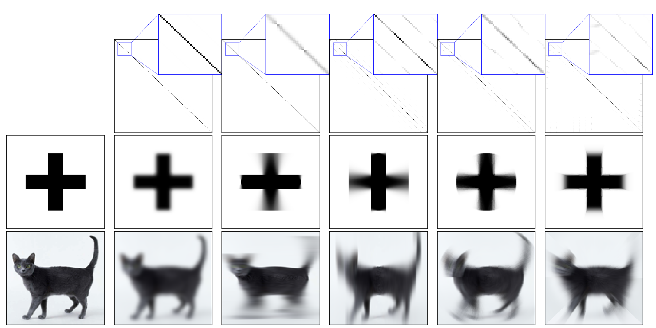
original

horizontal+vertical
translation

horizontal shear

vertical shear

rotation

zoom

Figure 2: Top row: matrix operator $\mathbb{E}_{\theta}[{\bm{M}}(\theta)]$ producing the expected image via $\mathbb{E}_{\theta}[{\bm{t}}(\theta)]=\mathbb{E}_{\theta}[{\bm{M}}(\theta)]{\bm{x}}$ (recall Eq. 6 and the discussion below Theorem 3.3), bottom block in Fig. 1) that transforms a (flattened) image into the average (expected) image after taking the expectation with respect to a given transformation distribution (as in Eq. 8), here with distributions: $\mathcal{N}(0,0.04)\otimes\mathcal{N}(0,0.04)$ for translation, $\mathcal{N}(0,0.2)$ for both shearing, $\mathcal{N}(0,0.1)$ for rotation and $\mathcal{N}(1,0.1)$ for zoom. This sparse matrix is the same regardless of the image and is derived in closed-form for the above standard transformations (Theorem 3.3). Middle & Bottom row: are two sample images (original on the left) that depict for each column the “expected image” under each transformation. Estimating those images (and any loss employing them) only through sampling the DA augmentations would require tens of thousands of samples (see Fig. 5).

3.1 Motivation: Current Data-Augmentation Training Performs Monte-Carlo Estimation

Training a model with DA consists in (i) sampling transformed images at each training iteration for each sample ${\bm{x}}_{n}$ as in $\mathcal{T}_{\theta_{n}}({\bm{x}}_{n})$ with $\theta_{n}\sim{\bm{\theta}}$ a randomly sampled DA parameter e.g. the amount of translation to apply, (ii) evaluating the loss $\mathcal{L}$ on the transformed sample/mini-batch/dataset, and (iii) using some flavor of gradient descent to update the parameters $\gamma$ of the model $f_{\gamma}$.

This training procedure corresponds to a one-sample Monte-Carlo (MC) estimate (Metropolis et al., 1953; Hastings, 1970) of the expected loss

$$\sum_{n=1}^{N}\mathbb{E}_{{\bm{\theta}}}\left[\mathcal{L}\left(f_{\gamma}(\mathcal{T}_{{\bm{\theta}}}({\bm{x}}_{n})\right)\right]\approx\sum_{n=1}^{N}\mathcal{L}(f_{\gamma}(\mathcal{T}_{\theta_{n}}({\bm{x}}_{n})),$$ (2)

with $\theta_{n}$ i.i.d samples from ${\bm{\theta}}$. In a supervised setting, the loss would also receive a per-sample target ${\bm{y}}_{n}$ as input. Although a one-sample estimate might be insufficient to apply the central limit theorem (Rosenblatt, 1956) and guarantee training convergence, the combination of multiple samples in each mini-batch and the repeated i.i.d sampling at each training step does provide convergence in most cases. For example, Self-Supervised losses i.e. losses that heavily rely on DA, tend to diverge is the mini-batch size is not large enough, as opposed to supervised losses. To avoid such instabilities, and to incorporate all the DA transformations of ${\bm{x}}_{n}$ into the model’s parameter update, one would be tempted to compute the model parameters’ gradient on the expected loss (left-hand side of Eq. 2) (see Section 3.4). Knowledge of the expected loss would also prove useful to measure the quality of the MC estimate (see Section 4.1).

As the closed-form expected loss requires knowledge of the expectation and variance of the transformed sample $\mathcal{T}_{{\bm{\theta}}}({\bm{x}}_{n})$, we first propose to formulate a novel and tractable augmentation model (Section 3.2) that will allow us to obtain those moments analytically (Section 3.3).

3.2 Proposed Data-Space Transformation

Instead of altering the coordinate positions of an image, as done in the coordinate-space transformation of Eq. 1, we propose to alter the image basis functions.

Going back to the construction of functions, one easily recalls that any (image) function can be expanded into its basis as in

$$I(u,v)=\int I(x,y)\delta(u-x,v-y)dxdy,$$

with $\delta$ the usual Dirac distributions. Suppose for now that we consider a horizontal translation by a constant $\theta$. Then, one can obtain that translated image $T$ via

$$T(u,v)=\int I(x,y)\delta(u-x-\theta,v-y)dxdy,$$ (3)

hence by moving the basis functions onto which the image is evaluated, rather than by moving the image’s coordinate. As the image is now constant with respect to the transformation parameter $\theta$, and as the basis functions have some specific analytical forms, the derivation of the transformed images expectation and variance, under random $\theta$, will become straightforward. Because the transformed image $T$ is now obtained by combining its pixel values (recall Eq. 3) we coin this transform as Data-Space Transform (DST) and we formally define it below.

Definition 3.1 (Data-Space Transform).

We define the data-space transformation of an image $I\in L^{2}(\mathbb{R}^{2})$ producing the transformed image $T\in L^{2}(\mathbb{R}^{2})$ as

$$T(u,v)=\int I(x,y)h_{\theta}(u,v,x,y)dxdy,$$ (4)

with $h_{\theta}(u,v,.,.)\in\mathbb{C}^{\infty}_{0}(\mathbb{R}^{2})$ encoding the transformation.

In Definition 3.1, we only impose for $h_{\theta}(u,v,.,.)$ to be with compact support. In fact, one should interpret $h_{\theta}(u,v,.,.)$ as a distribution whose purpose is to evaluate $I$ at a desired (coordinate) position on its domain. This evaluation -depending on the form of $h_{\theta}(u,v,.,.)$- can return a single pixel-value of the image $I$ at a desired location (as in Eq. 3), or it can combine multiple values e.g. with $h_{\theta}(u,v,.,.)$ being a bump function.

Coordinate-space transformations as DSTs. The coordinate-space transformation and the proposed DST (Definition 3.1) act in different spaces: the image input space and the image output space, respectively. Nevertheless, this does not limit the range of transformations that can be applied to an image. The following statement provides a simple recipe to turn any already employed coordinate-space transformation into a data-space one.

Proposition 3.2.

Any coordinate-space transformation (1) using $t:\mathbb{R}^{2}\mapsto\mathbb{R}^{2}$ can be expressed as a data-space transformation (4) by setting $h(u,v,x,y)=\delta(t(x,y)-[u,v]^{T})$.

Although we will focus here on the standard zoom/rotation/translation/…transformations, we propose in Appendix B a discussion on extending our results to DAs such as CutMix (Yun et al., 2019), CutOut (DeVries & Taylor, 2017) or MixUp (Zhang et al., 2017). Using Proposition 3.2, we obtain the DST operators $h_{\theta}(u,v,x,y)$ to be

$$\delta(u-x+\theta_{1},v-y+\theta_{2}),$$

$$\delta(u-x-\theta_{1}y,v-y-\theta_{2}x),$$

$$\delta(u-\theta x,v-\theta y),$$

$$\delta(u-\cos(\theta)x+\sin(\theta)y,v-\sin(\theta)x-\cos(\theta)y),$$ (5)

for the vertical/horizontal translation, vertical/horizontal shearing, zoom and rotation respectively. Before focusing on the analytical moments of the data-space transformed samples, we describe how those operators are applied in a discrete setting.

Discretized version. We now describe how any DST of a discrete image, flattened as a vector, can be expressed as a matrix-vector product with the matrix entries depending on the employed DA and its parameter $\theta$, as in Fig. 1. The functional form of the proposed transform in Eq. 4 producing the target image at a specific position $T(u,v)$ is linear in the image $I$. The continuous integral over the image domain is replaced with a summation with indices based on the desired sampling/resolution of $I$. Expressing linear operators as matrix-vector products will greatly ease our development, we will denote by ${\bm{x}}\in\mathbb{R}^{hw}$ the flattened $(h\times w)$ discrete images $I$. Hence, our data-space transformation, given some parameters $\theta$, takes the form of

$${\bm{t}}(\theta)={\bm{M}}(\theta){\bm{x}},$$ (6)

with ${\bm{t}}(\theta)\in\mathbb{R}^{hw}$ the flattened transformed image (which can be reshaped as desired) and ${\bm{M}}(\theta)\in\mathbb{R}^{hw\times hw}$ the matrix whose rows encode the discrete and flattened $h_{\theta}(u,v,.,.)$. For example, and employing a uniform grid sampling for illustration, ${\bm{M}}(\theta)_{i,j}=h_{\theta}(i//w,i\%w,j//w,j\%w)$ with $//$ representing the floor division and $\%$ the modulo operation. For the case of multi-channel images, we consider without loss of generality that the same transformation is applied on each channel separately. We depict this operation along with the exact form of ${\bm{M}}(\theta)$ for the case of the zoom transformation in Fig. 1.

3.3 Analytical Expectation and Variance of Transformed Images

The above construction (Definition 3.1) turns out to make the analytical form of the first two moments of an augmented sample straightforward to derive. As this contributes to one of our core contribution, we propose a step-by-step derivation of $\mathbb{E}_{{\bm{\theta}}}\left[\mathcal{T}_{{\bm{\theta}}}(I)\right]$ for the case of horizontal translation (as in Eq. 3).

Let’s consider again the continuous model (the discrete version is provided after Theorem 3.3). Using Fubini’s theorem to switch the order of integration and recalling Eq. 4, we have that

$$\mathbb{E}_{{\bm{\theta}}}\left[\mathcal{T}_{{\bm{\theta}}}(I)(u,v)\right]=\int I(x,y)\mathbb{E}_{{\bm{\theta}}}\left[h_{{\bm{\theta}}}(u,v,x,y)\right]dxdy.$$ (7)

Using the definition for $h$ from Eq. 5 for horizontal translation, $\mathbb{E}_{{\bm{\theta}}}\left[h_{\theta}(u,v,x,y)\right]$ becomes

$$\mathbb{E}_{{\bm{\theta}}}\left[\delta(u-x-\theta,v-y)\right]= \int\delta(u-x-\theta,v-y)p(\theta)d\theta$$

$$= p(u-x)\delta(v-y),$$

with $p$ the density function of ${\bm{\theta}}$ prescribing how the translation parameter is distributed. As a result, in this univariate translation case, the expected augmented image at coordinate $(u,v)$ is given by

$$\mathbb{E}_{{\bm{\theta}}}\left[\mathcal{T}_{{\bm{\theta}}}(I)(u,v)\right] =\int I(x,y)p(u-x)\delta(v-y)dxdy$$

$$=\int I(x,v)p(u-x)dx,$$ (8)

which can be further simplified into $\mathbb{E}_{{\bm{\theta}}}\left[\mathcal{T}_{{\bm{\theta}}}(I)(.,v)\right]=I(.,v)\star p$. Hence, the expected translated image is the convolution (on the $x$-axis only) between the original image $I$ and the univariate density function $p$. We formalize this for the transformations of Eq. 5 below.

Theorem 3.3.

The analytical form of $\mathbb{E}_{{\bm{\theta}}}\left[h_{{\bm{\theta}}}(u,v,x,y)\right]$, used to obtain the expected transformed image (recall Eq. 7) is given by

$$p(u-x,v-y)\text{ and }p\left(\frac{u}{x}\right)\delta\Big{(}\frac{u}{x}-\frac{v}{y}\Big{)},$$ (9)

for translation and rotation, other cases and $\mathbb{E}_{{\bm{\theta}}}[\mathcal{T}_{{\bm{\theta}}}({\bm{x}}_{n})\mathcal{T}_{{\bm{\theta}}}({\bm{x}}_{n})^{T}]$ are deferred to the appendix due to space limitation. (Proof in Appendix E.)

Notice for example how the expected image under random $2$-dimensional translations with ($2$-dimensional) density $p$ is given by the convolution $I\star p$, providing a new portal to study and interpret convolutions with nonnegative, sum-to-one filters $p$. Again, and as per Eq. 6, the discretized version of the expected image takes the form of $\mathbb{E}_{{\bm{\theta}}}[{\bm{t}}({\bm{\theta}})]=\mathbb{E}_{{\bm{\theta}}}[{\bm{M}}({\bm{\theta}})]{\bm{x}}$ with the entries of $\mathbb{E}_{{\bm{\theta}}}[{\bm{M}}({\bm{\theta}})]$ given by discretizing Eq. 9. We depict this expected matrix for various transformations as well as their application onto two different discrete images in Fig. 2, and we now proceed on deriving the left-hand side of Eq. 2 i.e. the explicit DA regularizer.

3.4 The Explicit Regularizer of Data-Augmentations

third          second          first

rotation

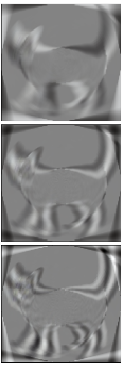
shear

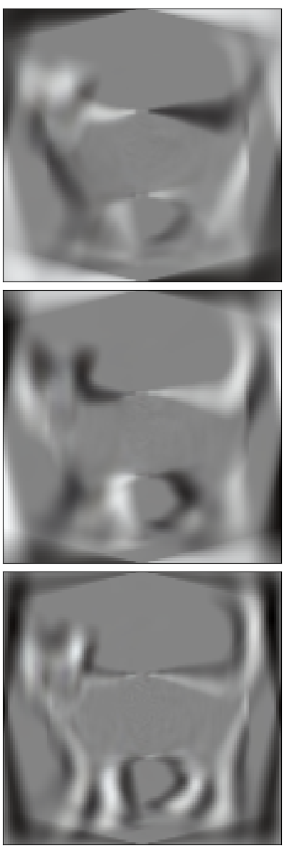
rank of $\mathbb{V}[\mathcal{T}({\bm{x}})]$

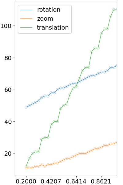
transformation amplitude

Figure 3: Left:Eigenvectors (${\bm{Q}}$ matrix in Theorem 3.4) associated to the largest eigenvalues of the sample variance matrix $\mathbb{V}[\mathcal{T}({\bm{x}})]$ for the rotation and shear augmentations with $\mathcal{U}(-15^{\circ},15^{\circ})$ and $\mathcal{U}(-15^{\circ},15^{\circ})\otimes\mathcal{U}(-15^{\circ},15^{\circ})$ respectively. As per Theorem 4.1, during training, aligning the kernel of the model’s Jacobian matrix (evaluated at each expected sample) to the largest eigenvectors of $\mathbb{V}[\mathcal{T}({\bm{x}})]$ (as seen above) will reduce the loss variance under the respective DA sampling. Right: the number of nonzero eigenvalues of $\mathbb{V}[\mathcal{T}({\bm{x}})]$ (nonzero elements in $\Lambda$ in Theorem 3.4) for increasing transformation amplitude (the datum dimension is $114\times 114\times 3$). We observe that even for high amplitude transformations, the constraint of Eq. 13 focus on a small umber of dimensions as standard DA span a low-dimensional subspace around each image, increasing linearly with the amplitude of the transformation.

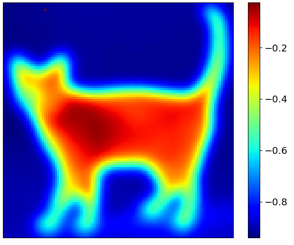
Figure 4: Pixel variance i.e. diagonal of $\mathbb{V}[\mathcal{T}({\bm{x}})]$ (left) and pixel covariance between a background pixel and all other pixels, i.e. $700^{\rm th}$ row of $\mathbb{V}[\mathcal{T}({\bm{x}})]$ (right) reshaped as an image for the cat of Fig. 2, for $\mathcal{T}$ translations with distribution $\mathcal{N}(0,0.1)\otimes\mathcal{N}(0,0.1)$. As per Theorem 3.4, the variance of the pixel values, seen on the left, being much higher for the edges of the cat than for its interior body/texture means that the parameters, during training, will be focusing on the cat texture, a phenomenon empirically observed in deep networks (Geirhos et al., 2019).

To keep notations as light as possible, we (for now) consider a linear regression model with Mean Squared Error (MSE). In that setting, the expected loss under DA sampling (recall Eq. 2) becomes

$$\mathcal{L}=\sum_{n=1}^{N}\mathbb{E}_{{\bm{\theta}}}\left[\left\|{\bm{y}}_{n}-{\bm{W}}\mathcal{T}_{{\bm{\theta}}}({\bm{x}}_{n})-{\bm{b}}\right\|_{2}^{2}\right],$$ (10)

with ${\bm{x}}_{n}\in\mathbb{R}^{D},n=1,\dots,N$ the input (flattened) n^th image $I_{n}$, ${\bm{y}}_{n}\in\mathbb{R}^{K}$ the n^th target vector, and ${\bm{W}}\in\mathbb{R}^{K\times D},{\bm{b}}\in\mathbb{R}^{K}$ the model’s parameters. Recall from Section 3.1 that to learn ${\bm{W}},{\bm{b}}$ under DA, the current method consists in performing a one-sample MC estimation. Instead, let’s derive (detailed derivation in Appendix C) the exact loss of Eq. 10 as a function of the sample mean and variance under the consider DA. We will drop the ${\bm{\theta}}$ subscript for clarity to obtain $\mathcal{L}$ as

$$\sum_{n=1}^{N}\|{\bm{y}}_{n}-{\bm{W}}\mathbb{E}\left[\mathcal{T}({\bm{x}}_{n})\right]-{\bm{b}}\|_{2}^{2}+\|{\bm{W}}{\bm{Q}}({\bm{x}})\Lambda({\bm{x}})^{\frac{1}{2}}\|_{F}^{2},$$ (11)

with the spectral decomposition ${\bm{Q}}({\bm{x}})\Lambda({\bm{x}}){\bm{Q}}({\bm{x}})^{T}=\mathbb{V}\left[\mathcal{T}({\bm{x}})\right]$. The right term in Eq. 11 is the explicit DA regularizer. It pushes the kernel space of ${\bm{W}}$ to align with the largest principal directions of the data manifold tangent space, as modeled by the DA. In fact, the largest eigenvectors in ${\bm{Q}}({\bm{x}})$ represent the principal directions of the data manifold tangent space at ${\bm{x}}$, as encoded via $\mathbb{V}\left[\mathcal{T}({\bm{x}})\right]$.

We propose in Fig. 3 visualization of ${\bm{Q}}$ and $\Lambda$ for different DAs, illustrating how each DA policy impacts the model’s parameter ${\bm{W}}$ through the regularization of Eq. 11. The knowledge of $\mathbb{E}\left[\mathcal{T}({\bm{x}})\right]$ and $\mathbb{V}\left[\mathcal{T}({\bm{x}})\right]$ from Theorem 3.3 finally enables to train a (linear) model on the true expected loss (Eq. 11) as we formalize below.

Theorem 3.4.

Training a linear model with MSE and infinite DA sampling is equivalent to minimizing Eq. 11 and produces the optimal ${\bm{W}}^{*}$ model’s parameter

$$\big{(}\sum_{n}({\bm{y}}_{n}-{\bm{b}})\mathbb{E}[{\bm{x}}_{n}]^{T}\big{)}\big{(}\sum_{n}\mathbb{E}\left[{\bm{x}}_{n}\right]\mathbb{E}\left[{\bm{x}}_{n}\right]^{T}+\mathbb{V}[{\bm{x}}_{n}]\big{)}^{-1},$$

with $\mathbb{E}({\bm{x}})\triangleq\mathbb{E}[\mathcal{T}({\bm{x}}_{n})]$ and $\mathbb{V}({\bm{x}})\triangleq\mathbb{V}[\mathcal{T}({\bm{x}}_{n})]$. We visualize $\mathbb{V}[{\bm{x}}_{n}]$ for the translation DA in Fig. 4.

The same line of result can be derived in the nonlinear setting by assuming that the DA is restricted to small transformations. In that case, one leverages a truncated Taylor approximation of the nonlinear model and recovers that (local) DA applies the same regularization than in Eq. 11 but with the model’s Jacobian matrix ${\bm{J}}f_{\gamma}({\bm{x}}_{n})$ in-place of ${\bm{W}}$ (more details in Section 4.3).

As we are now in possession of the exact expected loss, we are able to measure precisely how accurate were the MC estimate commonly used to train models under DA sampling which we propose to do in the following section.

4 Data-Augmentation Sampling Efficiency and Loss Sensitivity

In this section we present the empirical convergence of the loss MC estimate against the true expected loss (Section 4.1), and we provide exact variance analysis of that estimate as a function of the model’s Jacobian matrix and the sample variance eigenvectors (Section 4.2).

4.1 Empirical Monte-Carlo Convergence of Transformed Images

Now equipped with the closed-form formula for the average image and average loss under different image transformation distributions, we propose to empirically measure how efficient is the MC estimation to estimate the exact loss at-hand (recall Eq. 2).

We first propose in Fig. 5 a constructed $(64\times 64)$ image for which we compute the expected loss (Eq. 11) and the Monte-Carlo estimate (right-hand side of Eq. 2). Surprisingly, we obtain that even for a simple augmentation policy such as local translations, between 1000 and 10000 samples are required to correctly estimate the MSE loss from the augmented samples. In a more practical scenario, one could rightfully argue that the combination of the DA samples from different images allows to obtain a better estimate with a smaller amount of augmentations per sample. Hence, we provide in Fig. 6 that experiment using a linear model on MNIST with varying train set size. We observe that as the number of samples grows as the required number of augmentation per sample reduces. Nevertheless, even with thousands of samples, at least $50$ augmentations per sample are required to provide an accurate estimate.

We now propose to specifically quantify the sensitivity of the MC estimate to DA sampling.

4.2 Loss Sensitivity Under Data-Augmentation Sampling in the Linear and Nonlinear Regime

original image

expected
$E_{{\bm{\theta}}}[T_{{\bm{\theta}}}({\bm{x}})]$

estimated
$(N=100)$

estimated
$(N=10000)$

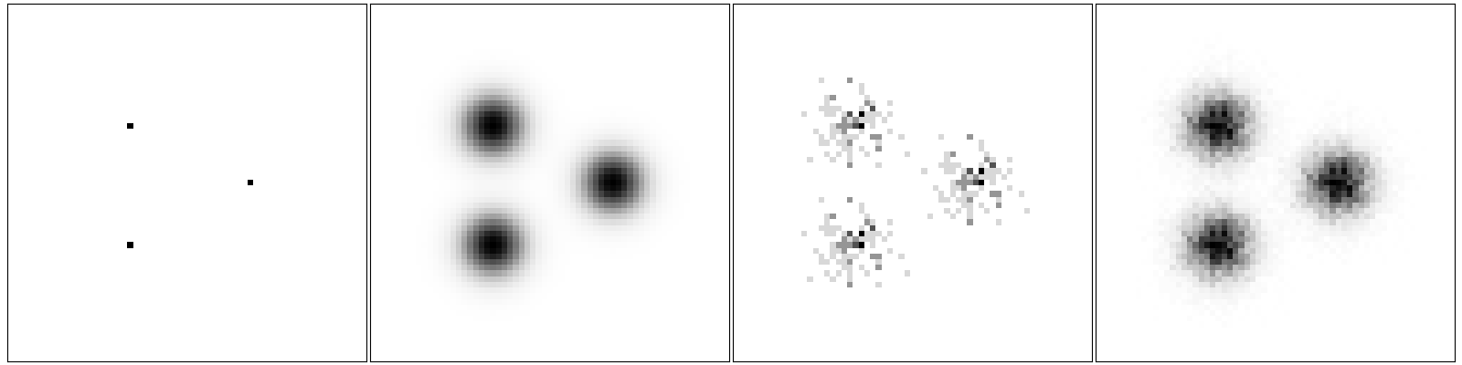
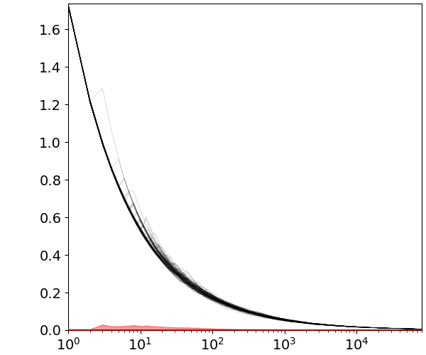
$\ell_{2}$ between MC estimate and the expected image (left) and the expected MSE loss (right) $N$ (log-scale) $N$ (log-scale)

Figure 5: Depiction of the analytical expected image under translation ($\mathcal{N}(0,0.1)\otimes\mathcal{N}(0,0.1)$) against its $N$-sample Monte-Carlo estimate (top row), $\ell_{2}$ distance between the true and estimated images (bottom left) and the true and estimated MSE loss with a random Gaussian ${\bm{y}},{\bm{W}}$ (bottom right). In red is depicted the standard deviation of the independent Monte-Carlo runs. Clearly we observe that even on a simple $(64\times 64)$ image and using the translation transformation, thousands of sampled images are necessary to provide an accurate estimate of the loss at hand. That is, sampling based data-augmentations are a rather inefficient medium to employ for injecting prior information into a model as this prior information will only emerge after tens of thousands of images have been sampled.

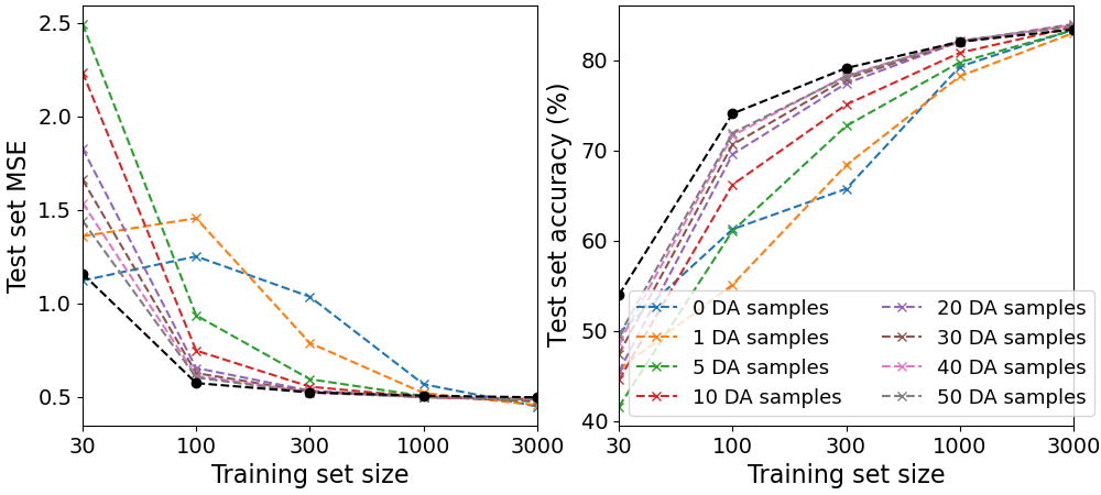
Figure 6: Linear regression task on the MNIST dataset with controlled training set size and translation DA sampling against the use of the expected loss (black line) for varying number of DA samples (colored lines). Evaluation is done on the one-hot encoded labels with the MSE (top) and on the accuracy performance (bottom) on the full MNIST test set. We observe that in low training data regime even a $50\times$ increase in dataset size obtained for DA sampling is not enough to provide the performances reached by employing the analytical expected loss. As the training size increases, as the DA samples get redundant with the added samples closing the performance gap.

Recalling Section 3.1, current DA training is performed on a MC estimate of the loss. The estimator’s variance (Newman & Barkema, 1999) is proportional to the variance of the quantity being estimated: $\mathbb{V}[(\mathcal{L}\circ f)(\mathcal{T}({\bm{x}}))]$. In this section, our goal is to characterize that variance precisely to understand when, and why, would an MC estimator converge for a given model.

By leveraging the delta method (Doob, 1935; Oehlert, 1992) i.e. a truncated Taylor expansion of the model and loss function mapping as $\mathcal{L}\circ f$, we have

$$\mathbb{V}[(\mathcal{L}\circ f)(\mathcal{T}({\bm{x}}))]\approx \|\nabla(\mathcal{L}\circ f)(\mathbb{E}[\mathcal{T}({\bm{x}})])\|^{2}_{\mathbb{V}[\mathcal{T}({\bm{x}})]},$$ (12)

with $\|{\bm{u}}\|^{2}_{{\bm{A}}}\triangleq{\bm{u}}^{T}{\bm{A}}{\bm{u}}$. Noticing that $\mathbb{V}[\mathcal{T}({\bm{x}})]=\mathbb{E}[\mathcal{T}({\bm{x}})\mathcal{T}({\bm{x}})^{T}]-\mathbb{E}[\mathcal{T}({\bm{x}})]\mathbb{E}[\mathcal{T}({\bm{x}})]^{T}$ and using the closed-form moments of augmented samples from Theorem 3.3, it is possible to write out Eq. 12 explicitly for model and DA specific analysis. We visualize $\mathbb{V}[\mathcal{T}({\bm{x}})]$ in Fig. 4.

Linear regression case. To gain some insight into Eq. 12, let’s first consider the linear regression case leading to

$$\mathbb{V}[(\mathcal{L}\circ f)(\mathcal{T}({\bm{x}}))]\approx \|{\bm{y}}-{\bm{W}}\mathbb{E}[\mathcal{T}({\bm{x}})]-{\bm{b}}\|^{2}_{{\bm{W}}\mathbb{V}[\mathcal{T}({\bm{x}})]{\bm{W}}^{T}}.$$

Hence the estimated loss variance depends on the model predicting the correct output when observing the expected sample $\mathbb{E}[\mathcal{T}({\bm{x}})]$, and on the smallest right singular vectors of ${\bm{W}}$ to align with the largest eigenvectors of $\mathbb{V}[\mathcal{T}({\bm{x}})]$, echoing our observation below Eq. 11.

General case. Since the result from Eq. 12 holds in the general setting, we can generalize the above observation to the more general setting.

Theorem 4.1.

The variance of the loss’s MC estimate (recall Eq. 2) for an input ${\bm{x}}_{n}$ goes to $0$ if the loss gradient $\nabla\mathcal{L}(f(\mathbb{E}[\mathcal{T}({\bm{x}})]))$ goes to $0$, or if the kernel of the model’s Jacobian matrix ${\bm{J}}f(\mathbb{E}[\mathcal{T}({\bm{x}})])$ aligns with the largest eigenvectors of the sample variance $\mathbb{V}[\mathcal{T}({\bm{x}})]$.

We derive here the proof of the above statement. By starting from Eq. 12 and applying the Cauchy-Schwarz inequality two times we obtain

$$\mathbb{V}[(\mathcal{L}\circ f)(\mathcal{T}({\bm{x}}))] \leq\|\nabla\mathcal{L}(f(\mathbb{E}[\mathcal{T}({\bm{x}})]))\|_{2}^{4}$$

$$\times \|{\bm{J}}f(\mathbb{E}[\mathcal{T}({\bm{x}})])\mathbb{V}[{\bm{x}}]{\bm{J}}f(\mathbb{E}[\mathcal{T}({\bm{x}})])^{T}\|_{F}^{2},$$

and then, rewriting ${\bm{J}}f(\mathbb{E}[\mathcal{T}({\bm{x}})])\mathbb{V}[\mathcal{T}({\bm{x}}){\bm{J}}f(\mathbb{E}[\mathcal{T}({\bm{x}})])^{T}$ as $BB^{T}$ and using $\|BB^{T}\|_{F}\leq\|B\|_{F}^{2}$ we obtain

$$\overbrace{\mathbb{V}[(\mathcal{L}\circ f)(\mathcal{T}({\bm{x}}))]}^{\mathclap{\;\;\;\;\;\;\small\text{loss $\circ$ model variance under DA}}} \leq\|\overbrace{\nabla\mathcal{L}(f(\mathbb{E}[\mathcal{T}({\bm{x}})]))}^{\mathclap{\small\hskip 79.6678pt\text{loss gradient at model(expected image)}}}\|_{2}^{4}$$

$$\times \|\underbrace{{\bm{J}}f(\mathbb{E}[\mathcal{T}({\bm{x}})])}_{\mathclap{\small\text{model's jacobian at expected image}}}\underbrace{{\bm{Q}}({\bm{x}})\Lambda^{\frac{1}{2}}({\bm{x}})}_{\mathclap{\hskip 39.83368pt\small\text{DA data manifold tangent space}}}\|_{F}^{4},$$ (13)

with $\mathbb{V}[\mathcal{T}({\bm{x}})]={\bm{Q}}\Lambda^{\frac{1}{2}}\Lambda^{\frac{1}{2}}{\bm{Q}}^{T}$. From Eq. 13, and assuming that the model’s Jacobian does not collapse to $0$ as the training loss is being minimized, we obtain that as the model’s Jacobian matrix kernel space aligns with the eigenvectors associated with the largest eigenvalues of $\mathbb{V}[\mathcal{T}({\bm{x}})]$ as the loss variance diminishes, concluding the proof. From Eq. 13, it becomes direct to prove that when employing Resnet architectures (He et al., 2016), the loss variance will reduce only from the model minimizing the loss at hand, since the Jacobian matrix is always full-rank, preventing any minimization of $\|{\bm{J}}f(\mathbb{E}[\mathcal{T}({\bm{x}})]){\bm{Q}}({\bm{x}})\Lambda^{\frac{1}{2}}({\bm{x}})\|_{F}^{4}$.
Limitations. We shall highlight that the results of this section rely on the delta method to approximate the intractable left-hand side of Eq. 12 by replacing $(\mathcal{L}\circ f)$ with its Taylor expansion at each $\mathbb{E}[\mathcal{T}({\bm{x}})]$, truncated to the first two terms. However, this has been a good-enough approximation technique in many recent results that have been validated both theoretically and empirically (see footnote on page Fig. 4).

4.3 Explicit Loss Sensitivity Minimization Provably Recovers TangentProp

The expected loss (Eq. 2) has been derived in the linear regression setting (Eq. 11). But in a more general scenario, and as discussed below Theorem 3.4, this expectation might not be tractable and thus needs to be approximated e.g. based on a Taylor expansion of the loss and model, might be needed. Alternatively to using the approximated expectation, one could employ the usual MC estimate of the expectation (right-hand side of Eq. 2), and leverage the MC estimator variance obtained in Eq. 13 as a regularizer. We show here that both approaches are equivalent, and recovers a popular regularizer known as TangentProp (Simard et al., 1991). Although various extensions of TangentProp have been introduced (Chapelle et al., 2001; Rifai et al., 2011) no principled derivation of it have been yet proposed under the viewpoint of expectation approximation, as we propose below. Using the same argument as in Section 4.2, the expectation of a nonlinear transformation of a random variable ($\mathcal{T}({\bm{x}}_{n})$) can be approximated from the expectation of the Taylor expansion (detailed derivations in Appendix D)

$$\mathbb{E}[(\mathcal{L} \circ f)(\mathcal{T}({\bm{x}}))]\approx(\mathcal{L}\circ f)(\mathbb{E}[\mathcal{T}({\bm{x}})])$$

$$\;\;+\frac{1}{2}\|\underbrace{{\bm{U}}^{\frac{1}{2}}({\bm{x}}){\bm{V}}({\bm{x}})^{T}}_{\mathclap{\text{loss curvature at the model's output}}}{\bm{J}}f(\mathbb{E}[\mathcal{T}({\bm{x}})]){\bm{Q}}({\bm{x}})\Lambda({\bm{x}})^{\frac{1}{2}}\|_{F}^{2},$$

with the spectral decomposition of the Hessian matrix ${\bm{V}}({\bm{x}}){\bm{U}}({\bm{x}}){\bm{V}}^{T}({\bm{x}})=H\mathcal{L}(f(\mathbb{E}[\mathcal{T}({\bm{x}})])$. Leveraging the Cauchy-Schwarz inequality on the Frobenius norm we finally obtain the following loss upper-bound

$$(\mathcal{L}\circ f)(\mathbb{E}[\mathcal{T}({\bm{x}})])+\kappa({\bm{x}})\underbrace{\|{\bm{J}}f(\mathbb{E}[\mathcal{T}({\bm{x}})]){\bm{Q}}({\bm{x}})\Lambda({\bm{x}})^{\frac{1}{2}}\|_{F}^{2}}_{\mathclap{\text{TangentProp regularization}}},$$

with $\kappa({\bm{x}})\geq 0$. As a result, the TangentProp regularizer naturally appears when using a Taylor approximation of the expected loss, and it corresponds to adding an explicit loss variance regularization term (compare the TangentProp with Eq. 13). We thus obtained from first principles that TangentProp emerges naturally when considering the second order Taylor approximation of the expected loss given a DA.

5 Conclusions

In this paper, we proposed a novel set of mathematical tools (Sections 3.2 and 3.3) under which it is possible to study DA and to provably answer some of the remaining open questions around the efficiency and impact of DA to train a model. We first obtained the explicit regularizer produced by different DAs in Section 3.4. This led to the following observation: the kernel space of the ${\bm{W}}$ matrix is pushed to align with the largest eigenvectors of the sample covariance matrix. This was then studied in a more general setting in Section 4.2 for nonlinear models when characterizing the loss variance under DA sampling. We also observed that Monte-Carlo sampling of transformed images is highly inefficient (Section 4.1), even if similar training samples combine their underlying information within a dataset. Lastly, those derivations led us to provably derive a known regularizer -TangentProp- as being the natural minimizer of a model’s loss variance. We hope that the proposed analysis will inspire many future works e.g. provable deep network architecture design.

Appendix:
A Data-Augmentation Is Worth A Thousand Samples

The appendix provides additional supporting materials such as figures, proofs, and additional discussions.

Appendix A Additional Figures

We first propose a visual depiction of coordinate space image transformations in Fig. 7. We employ here the case of a zoom transformation on a randomly generated image for illustration purposes. It can be seen that the transformation acts by altering the position of the image coordinates, and then produce the estimated value of the image at those new coordinates through some interpolation schemes. The most simple strategy is to employ a nearest-neighbor estimate i.e. given the new coordinate, predict the value of the new image at that position to be the same as the pixel value of the closest coordinate. As the coordinate transformation is composed with the image interpolation scheme, it is intricate to obtain any analytical quantity such as the expected image, motivating our proposed pixel-space transformation.

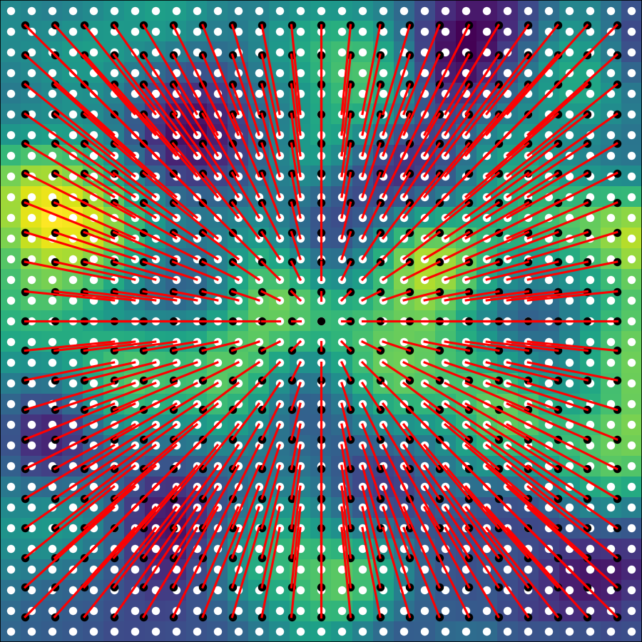
Figure 7: Depiction of the coordinate space transformation applied on a random image (white noise convolved with a low-pass filter. In this setting, one starts from the original image coordinates (white dots) and uses the mapping $t$ (recall Eq. 1) to know what coordinate $t(u,v)$ is associated to the target image coordinate $(u,v)$. In this example of a zoom transformation, the $t$ mapping will scale down those coordinates leading to a displacement (red lines) producing the black dots from the white ones. Once the new coordinates ($t(u,v)$) are known, the actual value is obtained through some flavors of interpolation between the white dots that are the closest to each black dot. For example, using the pixel value of the closest white dot corresponds to a nearest neighbor interpolation. Commonly, the 4 closest pixels are used with a bilinear weighting.

Appendix B Additional Data-Augmentations

The case of CutOut, CutMix or MixUp offer interesting avenues to our work. First, we shall highlight that those transformation perform both an alteration of the input ${\bm{x}}$ and of the corresponding output ${\bm{y}}$. Due to this double effect, they fall slightly out of the scope of this study.

Appendix C Expected Mean-Squared Error Derivation

In this section, we provide through direct derivations the expression of the expected mean squared error, under a given data augmentation distribution, as a function of the image first two moments. This result is crucial as it demonstrates that knowledge of those two moments is sufficient to obtain a closed form solution of the expected loss. As far as we are aware, this is a new result enabled by the proposed pixel-space transformation.

Using the cylic property of the Trace operator and the fact that $\mathbb{V}[\mathcal{T}({\bm{x}})]=\mathbb{E}[\mathcal{T}({\bm{x}})\mathcal{T}({\bm{x}})^{T}]-\mathbb{E}[\mathcal{T}({\bm{x}})]\mathbb{E}[\mathcal{T}({\bm{x}})]^{T}$ we can express the expected MSE loss as the MSE loss between the target and the expected input plus a regularization term as follows

$$\mathcal{L}({\bm{W}},{\bm{b}})= \sum_{n=1}^{N}\mathbb{E}_{\theta\sim\Theta}\left[\left\|{\bm{y}}_{n}-{\bm{W}}\mathcal{T}_{\theta}({\bm{x}}_{n})-{\bm{b}}\right\|_{2}^{2}\right]$$

$$= \sum_{n=1}^{N}\|{\bm{y}}_{n}-{\bm{b}}\|_{2}^{2}-2\langle{\bm{W}}^{T}({\bm{y}}_{n}-{\bm{b}}),\mathbb{E}_{\theta\sim\Theta}\left[\mathcal{T}_{\theta}({\bm{x}}_{n})\right]\rangle+\mathbb{E}_{\theta\sim\Theta}\left[\mathcal{T}_{\theta}({\bm{x}}_{n})^{T}{\bm{W}}^{T}{\bm{W}}\mathcal{T}_{\theta}({\bm{x}}_{n})\right]$$

$$= \sum_{n=1}^{N}\|{\bm{y}}_{n}-{\bm{b}}\|_{2}^{2}-2\langle{\bm{W}}^{T}({\bm{y}}_{n}-{\bm{b}}),\mathbb{E}_{\theta\sim\Theta}\left[\mathcal{T}_{\theta}({\bm{x}}_{n})\right]\rangle+\mathbb{E}_{\theta\sim\Theta}\left[{\rm Tr}\left({\bm{W}}^{T}{\bm{W}}\mathcal{T}_{\theta}({\bm{x}}_{n})\mathcal{T}_{\theta}({\bm{x}}_{n})^{T}\right)\right]\;\;\text{(cyclic prop.)}$$

$$= \sum_{n=1}^{N}\|{\bm{y}}_{n}-{\bm{b}}\|_{2}^{2}-2\langle{\bm{W}}^{T}({\bm{y}}_{n}-{\bm{b}}),\mathbb{E}_{\theta\sim\Theta}\left[\mathcal{T}_{\theta}({\bm{x}}_{n})\right]\rangle+{\rm Tr}\left({\bm{W}}^{T}{\bm{W}}\mathbb{E}_{\theta\sim\Theta}\left[\mathcal{T}_{\theta}({\bm{x}}_{n})\mathcal{T}_{\theta}({\bm{x}}_{n})^{T}\right]\right)\;\;\text{(linear prop.)}$$

$$= \sum_{n=1}^{N}\|{\bm{y}}_{n}-{\bm{b}}\|_{2}^{2}+\langle{\bm{W}}^{T}({\bm{y}}_{n}-{\bm{b}}),\mathbb{E}_{\theta\sim\Theta}\left[\mathcal{T}_{\theta}({\bm{x}}_{n})\right]\rangle$$

$$+{\rm Tr}\left({\bm{W}}^{T}{\bm{W}}\left(\mathbb{E}_{\theta\sim\Theta}\left[\mathcal{T}_{\theta}({\bm{x}}_{n})\mathcal{T}_{\theta}({\bm{x}}_{n})^{T}\right]-\mathbb{E}_{\theta\sim\Theta}\left[\mathcal{T}_{\theta}({\bm{x}}_{n})\right]\mathbb{E}_{\theta\sim\Theta}\left[\mathcal{T}_{\theta}({\bm{x}}_{n})\right]^{T}\right)\right)$$

$$+{\rm Tr}\left({\bm{W}}^{T}{\bm{W}}\left(\mathbb{E}_{\theta\sim\Theta}\left[\mathcal{T}_{\theta}({\bm{x}}_{n})\right]\mathbb{E}_{\theta\sim\Theta}\left[\mathcal{T}_{\theta}({\bm{x}}_{n})\right]^{T}\right)\right)$$

$$= \sum_{n=1}^{N}\|{\bm{y}}_{n}-{\bm{b}}\|_{2}^{2}+\langle{\bm{W}}^{T}({\bm{y}}_{n}-{\bm{b}}),\mathbb{E}_{\theta\sim\Theta}\left[\mathcal{T}_{\theta}({\bm{x}}_{n})\right]\rangle+{\rm Tr}\left({\bm{W}}^{T}{\bm{W}}\mathbb{E}_{\theta\sim\Theta}\left[\mathcal{T}_{\theta}({\bm{x}}_{n})\right]\mathbb{E}_{\theta\sim\Theta}\left[\mathcal{T}_{\theta}({\bm{x}}_{n})\right]^{T}\right)$$

$$+{\rm Tr}\left({\bm{W}}^{T}{\bm{W}}\mathbb{V}_{\theta\sim\Theta}\left[\mathcal{T}_{\theta}({\bm{x}}_{n})\right]\right)$$

$$= \sum_{n=1}^{N}\|{\bm{y}}_{n}-{\bm{W}}\mathbb{E}_{\theta\sim\Theta}\left[\mathcal{T}_{\theta}({\bm{x}}_{n})\right]-{\bm{b}}\|_{2}^{2}+{\rm Tr}\left({\bm{W}}^{T}{\bm{W}}\mathbb{V}_{\theta\sim\Theta}\left[\mathcal{T}_{\theta}({\bm{x}}_{n})\right]\right),$$

concluding our derivations. Notice how the regularization term acts upon the matrix ${\bm{W}}$ through the variance of the image under the specified transformation.

Appendix D Taylor Approximation

In this section we now describe how to exploit a second order Taylor approximation of any loss and/or transformation of the transformed image as a way to obtain an approximated expected loss/output. Without loss of generality we consider here this mapping to be $(\mathcal{L}\circ f)$, i.e. a nonlinear mapping $f$ and a loss function $\mathcal{L}$. The same result applies regardless of those mappings. The approximation will holds mostly for small transformation due to the quadratic approximation of the mapping.

Let’s first obtain the second order Taylor expansion of the nonlinear mapping at $\mathbb{E}[\mathcal{T}({\bm{x}})]$ as

$$(\mathcal{L}\circ f)(\mathcal{T}({\bm{x}}))\approx (\mathcal{L}\circ f)(\mathbb{E}[\mathcal{T}({\bm{x}})])+(\mathcal{T}({\bm{x}}_{n})-\mathbb{E}[\mathcal{T}({\bm{x}})])^{T}\nabla(\mathcal{L}\circ f)(\mathbb{E}[\mathcal{T}({\bm{x}})])$$

$$+\frac{1}{2}(\mathcal{T}({\bm{x}}_{n})-\mathbb{E}[\mathcal{T}({\bm{x}})])^{T}H(\mathcal{L}\circ f)(\mathbb{E}[\mathcal{T}({\bm{x}})])(\mathcal{T}({\bm{x}}_{n})-\mathbb{E}[\mathcal{T}({\bm{x}})])$$

notice that we are required to at least take the second order Taylor expansion as the first order will vanish as soon as we will take the expectation of that approximation. In fact, taking the expectation of the above, we obtain (using the cyclic property of the Trace operator)

$$\mathbb{E}[(\mathcal{L}\circ f)(\mathcal{T}({\bm{x}}))]\approx (\mathcal{L}\circ f)(\mathbb{E}[\mathcal{T}({\bm{x}})])+\frac{1}{2}{\rm Tr}\left(H(\mathcal{L}\circ f)(\mathbb{E}[\mathcal{T}({\bm{x}})])\mathbb{V}(\mathcal{T}({\bm{x}}))\right)$$

$$= (\mathcal{L}\circ f)(\mathbb{E}[\mathcal{T}({\bm{x}})])+\frac{1}{2}{\rm Tr}\left({\bm{J}}f_{\gamma}(\mathbb{E}[\mathcal{T}({\bm{x}})]^{T}H\mathcal{L}(f_{\gamma}(\mathbb{E}[\mathcal{T}({\bm{x}})]){\bm{J}}f_{\gamma}(\mathbb{E}[\mathcal{T}({\bm{x}})]\mathbb{V}(\mathcal{T}({\bm{x}}))\right)$$

$$= (\mathcal{L}\circ f)(\mathbb{E}[\mathcal{T}({\bm{x}})])+\frac{1}{2}\|{\bm{U}}^{\frac{1}{2}}({\bm{x}}){\bm{V}}({\bm{x}})^{T}{\bm{J}}f_{\gamma}(\mathbb{E}[\mathcal{T}({\bm{x}})]){\bm{Q}}({\bm{x}})\Lambda({\bm{x}})^{\frac{1}{2}}\|_{F}^{2},$$

where $H$ represents the Hessian. The above concludes our derivation that led to a generalization of the linear case. In fact, notice that in the linear with mean squared error the second order Taylor approximation is exact and the above is exactly the same as the one of the previous section.

Appendix E Proof of Thm. 3.3

This section provides the derivation of the first two moments of images under specific image transformations. Note that the actual distribution is abstracted away as simple $p$. In fact, those results do not depend on the specific form of $p$, rather, they depend on the type of transformation being applied e.g. rotation, translation or zoom. We thus propose to derive them, following the same recipe one will be able to obtain the analytical form of the first two moments for any desired transformation. One fact that we will heavily leverage is the fact that integrating a functional and a Dirac function can be expressed as evaluating that function as the position of the Dirac (recall Proposition 3.2).

Throughout this proof, we will denote by $T(u,v;\theta)$ the value of the transformed image at spatial position $(u,v)$, hence $\mathbb{E}_{\theta\sim\Theta}[T(u,v;\theta)]$ is the expected value of the transformed image at pixel position $(u,v)$. And $\mathbb{E}_{\theta\sim\Theta}[T(u,v;\theta)T(u^{\prime},v^{\prime};\theta)]$ is the second order (uncentered) moment representing the interplay between pixel positions $(u,v)$ and $(u^{\prime}v^{\prime})$ of the transformed image. This second order moment and the first order moment can be used to obtained the variance/covariance of the transformed image.

Vertical and Horizontal translation: The case of vertical and horizontal translations is taken care of jointly, for vertical-only or horizontal-only transformations, simply use a distribution that is a Dirac (at $0$) for the transformation that is not needed. We thus obtain in general given a $2$-dimensional density $p$ as

$$\mathbb{E}_{\theta\sim\Theta}[T(u,v;\theta)]= \int_{\theta}p(\theta)\int I(x,y)h_{\theta}(u,v,x,y)dxdyd\theta$$

$$= \int_{-\infty}^{\infty}p(\theta_{1},\theta_{2})\int I(x,y)\delta(u=x+\theta_{1},v=y+\theta_{2})dxdyd\theta$$

$$= \int I(x,y)\int_{-\infty}^{\infty}p(\theta_{1},\theta_{2})\delta(u=x+\theta_{1},v=y+\theta_{2})d\theta dxdy$$

$$= \int I(x,y)p(u-x,v-y)dxdy$$

from this we also directly obtain that the expected image can be expressed as a $2$-dimensional convolution between the original image and the density being employed for the translation as in $\mathbb{E}_{\theta\sim\Theta}[T(.,.;\theta)]=I\star p$. We now derive the second order moments

$$\mathbb{E}_{\theta\sim\Theta}[T(u,v;\theta)T(u^{\prime},v^{\prime};\theta)]= \int I(x,y)I(x^{\prime},y^{\prime})\int_{-\infty}^{\infty}p(\theta_{1},\theta_{2})\delta(u=x+\theta_{1},v=y+\theta_{2})$$

$$\times\delta(u^{\prime}=x^{\prime}+\theta_{1},v^{\prime}=y^{\prime}+\theta_{2})d\theta_{1}d\theta_{2}dxdydx^{\prime}dy^{\prime}$$

$$= \int I(x,y)I(x^{\prime},y^{\prime})p(u-x,v-y)\delta(v-y-(v^{\prime}-y^{\prime}))\delta(u-x-(u^{\prime}-x^{\prime}))dxdx^{\prime}dydy^{\prime}$$

$$= \int I(x^{\prime}-u^{\prime}+u,y^{\prime}-v^{\prime}+v)I(x^{\prime},y^{\prime})p(u-x^{\prime}+u^{\prime}-u,v-(y^{\prime}-v^{\prime}+v))dx^{\prime}dy^{\prime}$$

$$= \int I(x^{\prime}-u^{\prime}+u,y^{\prime}-v^{\prime}+v)I(x^{\prime},y^{\prime})p(-x^{\prime}+u^{\prime},-y^{\prime}+v^{\prime})dx^{\prime}dy^{\prime}$$

$$= \int I(a+u,b+v)I(a+u^{\prime},b+v^{\prime})p(-a,-b)dadb,$$

as a result the second order moment of the image at $(u,v)$ and ($u^{\prime},v^{\prime}$) is simply the inner product between the image translated to $(u,v)$, $(u^{\prime}v^{\prime})$ and the density $p$.

Vertical Shear: we now move on to the vertical shear transformation. Note that this transformation can be seen as a special case of a translate but with a translation coefficient varying with row/columns. We obtain the following derivations

$$\mathbb{E}_{\theta\sim\Theta}[T(u,v;\theta)]= \int_{\theta}p(\theta)\int I(x,y)h_{\theta}(u,v,x,y)dxdyd\theta$$

$$= \int_{\theta}p(\theta)\int I(x,y)\delta(u=x+\theta*v,v=y)dxdyd\theta$$

$$= \int I(x,y)\int_{-\infty}^{\infty}p(\theta)\delta(u=x+\theta*v,v=y)d\theta$$

$$= \int I(x,v)p(\frac{u-x}{v})dx$$

$$\implies\mathbb{E}_{\theta\sim\Theta}[T(.,v;\theta)]= I(.,v)\star p(\frac{.}{v}),$$

as a result we see that an efficient way to obtain the expected image (each row/column of it) is via a $1$-dimensional convolution with the density being rescaled based on the considered row/column. We now consider the second order moment below

$$\mathbb{E}_{\theta\sim\Theta}[T(u,v;\theta)T(u^{\prime},v^{\prime};\theta)]= \int I(x,y)I(x^{\prime},y^{\prime})\int_{-\infty}^{\infty}p(\theta)$$

$$\times\delta(u=x+\theta*v,v=y)\delta(u^{\prime}=x^{\prime}+\theta*v^{\prime},v^{\prime}=y^{\prime})dxdydx^{\prime}dy^{\prime}d\theta$$

$$= \int I(x,v)I(x^{\prime},v^{\prime})\int_{-\infty}^{\infty}p(\theta)\delta(u=x+\theta*v)\delta(u^{\prime}=x^{\prime}+\theta*v^{\prime})dxdx^{\prime}d\theta$$

$$= \int I(x,v)I(x^{\prime},v^{\prime})p(\frac{u-x}{v})\delta(\frac{u-x}{v}=\frac{u^{\prime}-x^{\prime}}{v^{\prime}})dxdx^{\prime}$$

$$= \int I(x,v)I(x^{\prime},v^{\prime})p(\frac{u-x}{v})\delta(x=u+(x^{\prime}-u^{\prime})\frac{v}{v^{\prime}})dxdx^{\prime}$$

$$= \int I(u+(x^{\prime}-u^{\prime})\frac{v}{v^{\prime}},v)I(x^{\prime},v^{\prime})p(\frac{u^{\prime}-x^{\prime}}{v^{\prime}})dx^{\prime}$$

$$= \int I(u+zv,v)I(u^{\prime}+zv^{\prime},v^{\prime})p(-z)v^{\prime}dz,$$

concluding the shearing transformation results. For the horizontal shear, simply do the above derivations with the image axes swapped.

Rotation:

$$\mathbb{E}_{\theta\sim\Theta}[T(u,v;\theta)]= \int_{\theta}p(\theta)\int I(x,y)h_{\theta}(u,v,x,y)dxdyd\theta$$

$$= \int_{\theta}p(\theta)\int I(x,y)\delta(u=\cos(\theta)x-\sin(\theta)y,v=\sin(\theta)x+\cos(\theta)y)dxdyd\theta$$

$$= \int_{\theta}p(\theta)\int I(x,y)\delta(x^{2}+y^{2}=u^{2}+v^{2},\theta=\arctan(y/x)-\arctan(v/u))dxdyd\theta$$

$$= \int I(x,y)\int_{\theta}p(\theta)\delta(x^{2}+y^{2}=u^{2}+v^{2},\theta=\arctan(y/x)-\arctan(v/u))dxdyd\theta$$

$$= \int I(x,y)p(\arctan(y/x)-\arctan(v/u))\delta(x^{2}+y^{2}=u^{2}+v^{2})dxdy$$

$$\mathbb{E}_{\theta\sim\Theta}[T(u,v;\theta)T(u^{\prime},v^{\prime};\theta)]= \int_{\theta}p(\theta)\int I(x,y)h_{\theta}(u,v,x,y)dxdy\int I(x^{\prime},y^{\prime})h_{\theta}(u^{\prime},v^{\prime},x^{\prime},y^{\prime})dx^{\prime}dy^{\prime}d\theta$$

$$= \int I(x,y)I(x^{\prime},y^{\prime})\int_{0}^{2\pi}p(\arctan(y/x)-\arctan(v/u))$$

$$\times\delta(\arctan(y/x)-\arctan(v/u)=\arctan(y^{\prime}/x^{\prime})-\arctan(v^{\prime}/u^{\prime}),$$

$$\;\;x^{2}+y^{2}=u^{2}+v^{2},x^{\prime 2}+y^{\prime 2}=u^{\prime 2}+v^{\prime 2})dxdydx^{\prime}dy^{\prime}$$

This concludes our derivations. Note that while we focused here on the most common transformations, the same recipe can be employed to obtain the expected transformed image for more complicated transformations.

References

- Baldi & Sadowski (2013) Baldi, P. and Sadowski, P. J. Understanding dropout. Advances in neural information processing systems, 26:2814–2822, 2013.
- Bouthillier et al. (2015) Bouthillier, X., Konda, K., Vincent, P., and Memisevic, R. Dropout as data augmentation. arXiv preprint arXiv:1506.08700, 2015.
- Chapelle et al. (2001) Chapelle, O., Weston, J., Bottou, L., and Vapnik, V. Vicinal risk minimization. Advances in neural information processing systems, pp. 416–422, 2001.
- DeVries & Taylor (2017) DeVries, T. and Taylor, G. W. Improved regularization of convolutional neural networks with cutout. arXiv preprint arXiv:1708.04552, 2017.
- Doob (1935) Doob, J. L. The limiting distributions of certain statistics. The Annals of Mathematical Statistics, 6(3):160–169, 1935.
- Geirhos et al. (2019) Geirhos, R., Rubisch, P., Michaelis, C., Bethge, M., Wichmann, F. A., and Brendel, W. Imagenet-trained CNNs are biased towards texture; increasing shape bias improves accuracy and robustness. In International Conference on Learning Representations, 2019. URL https://openreview.net/forum?id=Bygh9j09KX.
- Goodfellow et al. (2016) Goodfellow, I., Bengio, Y., and Courville, A. Deep learning. MIT press, 2016.
- Gunasekar et al. (2018) Gunasekar, S., Lee, J., Soudry, D., and Srebro, N. Implicit bias of gradient descent on linear convolutional networks. arXiv preprint arXiv:1806.00468, 2018.
- Hastings (1970) Hastings, W. K. Monte carlo sampling methods using markov chains and their applications. 1970.
- He et al. (2016) He, K., Zhang, X., Ren, S., and Sun, J. Identity mappings in deep residual networks. In European conference on computer vision, pp. 630–645. Springer, 2016.
- Heckbert (1982) Heckbert, P. Color image quantization for frame buffer display. ACM Siggraph Computer Graphics, 16(3):297–307, 1982.
- Hernández-García & König (2018a) Hernández-García, A. and König, P. Data augmentation instead of explicit regularization. arXiv preprint arXiv:1806.03852, 2018a.
- Hernández-García & König (2018b) Hernández-García, A. and König, P. Do deep nets really need weight decay and dropout? arXiv preprint arXiv:1802.07042, 2018b.
- Hernández-García & König (2018c) Hernández-García, A. and König, P. Further advantages of data augmentation on convolutional neural networks. In International Conference on Artificial Neural Networks, pp. 95–103. Springer, 2018c.
- Jaderberg et al. (2015) Jaderberg, M., Simonyan, K., Zisserman, A., et al. Spatial transformer networks. Advances in neural information processing systems, 28:2017–2025, 2015.
- LeJeune et al. (2019) LeJeune, D., Balestriero, R., Javadi, H., and Baraniuk, R. G. Implicit rugosity regularization via data augmentation. arXiv preprint arXiv:1905.11639, 2019.
- Mallat (1989) Mallat, S. G. Multifrequency channel decompositions of images and wavelet models. IEEE Transactions on Acoustics, Speech, and Signal Processing, 37(12):2091–2110, 1989.
- Metropolis et al. (1953) Metropolis, N., Rosenbluth, A. W., Rosenbluth, M. N., Teller, A. H., and Teller, E. Equation of state calculations by fast computing machines. The journal of chemical physics, 21(6):1087–1092, 1953.
- Misra & Maaten (2020) Misra, I. and Maaten, L. v. d. Self-supervised learning of pretext-invariant representations. In Proceedings of the IEEE/CVF Conference on Computer Vision and Pattern Recognition, pp. 6707–6717, 2020.
- Mukundan et al. (2001) Mukundan, R., Ong, S., and Lee, P. A. Image analysis by tchebichef moments. IEEE Transactions on image Processing, 10(9):1357–1364, 2001.
- Newman & Barkema (1999) Newman, M. E. and Barkema, G. T. Monte Carlo methods in statistical physics. Clarendon Press, 1999.
- Neyshabur (2017) Neyshabur, B. Implicit regularization in deep learning. arXiv preprint arXiv:1709.01953, 2017.
- Neyshabur et al. (2014) Neyshabur, B., Tomioka, R., and Srebro, N. In search of the real inductive bias: On the role of implicit regularization in deep learning. arXiv preprint arXiv:1412.6614, 2014.
- Oehlert (1992) Oehlert, G. W. A note on the delta method. The American Statistician, 46(1):27–29, 1992.
- Perez & Wang (2017) Perez, L. and Wang, J. The effectiveness of data augmentation in image classification using deep learning. arXiv preprint arXiv:1712.04621, 2017.
- Razin & Cohen (2020) Razin, N. and Cohen, N. Implicit regularization in deep learning may not be explainable by norms. arXiv preprint arXiv:2005.06398, 2020.
- Rifai et al. (2011) Rifai, S., Dauphin, Y. N., Vincent, P., Bengio, Y., and Muller, X. The manifold tangent classifier. Advances in neural information processing systems, 24:2294–2302, 2011.
- Rosenblatt (1956) Rosenblatt, M. A central limit theorem and a strong mixing condition. Proceedings of the National Academy of Sciences of the United States of America, 42(1):43, 1956.
- Sawchuk (1974) Sawchuk, A. A. Space-variant image restoration by coordinate transformations. JOSA, 64(2):138–144, 1974.
- Shorten & Khoshgoftaar (2019) Shorten, C. and Khoshgoftaar, T. M. A survey on image data augmentation for deep learning. Journal of Big Data, 6(1):1–48, 2019.
- Simard et al. (1991) Simard, P., Victorri, B., LeCun, Y., and Denker, J. S. Tangent prop-a formalism for specifying selected invariances in an adaptive network. In NIPS, volume 91, pp. 895–903. Citeseer, 1991.
- Soudry et al. (2018) Soudry, D., Hoffer, E., Nacson, M. S., Gunasekar, S., and Srebro, N. The implicit bias of gradient descent on separable data. The Journal of Machine Learning Research, 19(1):2822–2878, 2018.
- Srivastava et al. (2014) Srivastava, N., Hinton, G., Krizhevsky, A., Sutskever, I., and Salakhutdinov, R. Dropout: a simple way to prevent neural networks from overfitting. The journal of machine learning research, 15(1):1929–1958, 2014.
- Taqi et al. (2018) Taqi, A. M., Awad, A., Al-Azzo, F., and Milanova, M. The impact of multi-optimizers and data augmentation on tensorflow convolutional neural network performance. In 2018 IEEE Conference on Multimedia Information Processing and Retrieval (MIPR), pp. 140–145. IEEE, 2018.
- Tikhonov (1943) Tikhonov, A. N. On the stability of inverse problems. In Dokl. Akad. Nauk SSSR, volume 39, pp. 195–198, 1943.
- Unser (2019) Unser, M. A representer theorem for deep neural networks. J. Mach. Learn. Res., 20(110):1–30, 2019.
- Wang et al. (2018) Wang, Z., Balestriero, R., and Baraniuk, R. A max-affine spline perspective of recurrent neural networks. In International Conference on Learning Representations, 2018.
- Wei et al. (2020) Wei, C., Kakade, S., and Ma, T. The implicit and explicit regularization effects of dropout, 2020.
- Wolberg & Zokai (2000) Wolberg, G. and Zokai, S. Robust image registration using log-polar transform. In Proceedings 2000 International Conference on Image Processing (Cat. No. 00CH37101), volume 1, pp. 493–496. IEEE, 2000.
- Yun et al. (2019) Yun, S., Han, D., Oh, S. J., Chun, S., Choe, J., and Yoo, Y. Cutmix: Regularization strategy to train strong classifiers with localizable features. In Proceedings of the IEEE/CVF International Conference on Computer Vision, pp. 6023–6032, 2019.
- Zbontar et al. (2021) Zbontar, J., Jing, L., Misra, I., LeCun, Y., and Deny, S. Barlow twins: Self-supervised learning via redundancy reduction. arXiv preprint arXiv:2103.03230, 2021.
- Zhang et al. (2021) Zhang, C., Bengio, S., Hardt, M., Recht, B., and Vinyals, O. Understanding deep learning (still) requires rethinking generalization. Communications of the ACM, 64(3):107–115, 2021.
- Zhang et al. (2018) Zhang, G., Wang, C., Xu, B., and Grosse, R. Three mechanisms of weight decay regularization. arXiv preprint arXiv:1810.12281, 2018.
- Zhang et al. (2017) Zhang, H., Cisse, M., Dauphin, Y. N., and Lopez-Paz, D. mixup: Beyond empirical risk minimization. arXiv preprint arXiv:1710.09412, 2017.