Causal Process Mining from Relational Databases
with Domain Knowledge

Abstract

The plethora of algorithms in the research field of process mining builds on directly-follows relations. Even though various improvements have been made in the last decade, there are serious weaknesses of these relationships. Once events associated with different objects that relate with a cardinality of 1:N and N:M to each other, techniques based on directly-follows relations produce spurious relations, self-loops, and back-jumps. This is due to the fact that event sequence as described in classical event logs differs from event causation. In this paper, we address the research problem of representing the causal structure of process-related event data. To this end, we develop a new approach called Causal Process Mining. This approach renounces the use of flat event logs and considers relational databases of event data as an input. More specifically, we transform the relational data structures based on the Causal Process Template into what we call Causal Event Graph. We evaluate our approach and compare its outputs with techniques based on directly-follows relations in a case study with an European food production company. Our results demonstrate the benefits for enriching process mining with additional knowledge from the domain.

1 Introduction

Process Mining (PM) is a research field focusing on the development of automatic analysis techniques that provide insights into business processes based on event data [1]. Over the last decade, PM research has spent considerable efforts on improving algorithms for automatic process discovery. Notable advancements of recent algorithms include the inductive miner [2], the evolutionary tree miner [3], or the split miner [4]. These algorithms differ in their balance between fitness, simplicity, generalization, and precision in order to better cope with different event log characteristics or use cases [1, 5], but they have in common that they build on event logs as input and directly-follows relations for generating models.

Even though most PM techniques build on event logs and directly-follows relations, they exhibit some serious weaknesses. Once events associated with different objects that relate with a cardinality of 1:N and N:M to each other, techniques based on directly-follows relations produce spurious relations, self-loops, and back-jumps. The incapability to handle such cardinality constitutes a representational bias [6, 7] that causes problems for appropriately representing, a.o., logistic processes [8]. Here, interacting objects cannot be traced using a single case identifier. Recent works on artifact-related PM [9] or object-centric PM [10, 11] as well as approaches that consider relational databases [12, 13, 14] or multi-dimensional event data [15] address the problem by associating a single event with one or more objects. However, they do not exploit causal domain knowledge such as visible in the foreign key relationships of the databases storing event data. This is a fundamental problem, because it is not possible to reconstruct causal relationships from observation of behavior alone [16]. As a consequence, techniques based on Directly-Follows Graphs (DFGs) produce connections that are not causal, yielding overly complex models.

In this paper, we address the problem of representing the causal structure of process-related event data. To this end, we develop a new approach called Causal Process Mining (CPM). This approach renounces the use of flat event logs and considers relational databases of event data as well as causal knowledge as an input. More specifically, we transform the relational data structures based on the Causal Process Template (CPT) into what we call Causal Event Graph (CEG). In turn, these CEGs can be stored in a graph database and they can be aggregated to models that we call Aggregated Causal Event Graphs (ACEGs). CPM exploits these structures and offers multiple operations to investigate the process from various perspectives and at different levels of aggregation. With the CPT, we propose a novel component that helps to integrate alternative knowledge sources. Moreover, we evaluate CPM and compare its outputs with techniques based on directly-follows relations in a case study with an European food production company. Our results demonstrate that directly-follows miners produce a large number of spurious relationships, which our approach captures correctly.

The rest of the paper is structured as follows. Section 2 illustrates the fundamental problem of DFGs by making use of a production scenario example. Based on this discussion, we derive requirements for representing the corresponding class of scenarios appropriately. Section 3 defines our approach of CPM. We illustrate how our approach handles cardinality, causality, and process instance aggregation. Section 4 conducts an evaluation by comparing the CPM approach to common DFG approaches as well as discusses the requirements in the context of related work. Section 5 concludes the paper with a summary and an outlook on future research.

2 Background

In this section, we illustrate the research problem and relate it to Pearl’s three-level causal hierarchy [16]. Upon this basis, we identify four requirements for addressing the problem of representing the causal structure based on event data. Using these requirements, we compare contributions from prior research.

2.1 Problem statement

This section describes the problem of PM approaches that use event logs with a single case identifier for generating DFGs. Extracting directly-follows relations and representing them as a graph is the “de facto standard” [17, p. 324] of both commercial tools and the main share of the academic implementations.

Let us look at the different technical steps of conducting a PM analysis according to this de facto approach. Event logs stem from transactions that are executed by humans or by software systems. These transactions are typically persisted in tables of relational databases, which themselves are connected by foreign-key relations of different cardinalities. As a preparation for PM, a process analyst creates an event log by defining the obligatory case identifier, specifying the process activities, and related properties such as resources, timestamps, or business objects [18]. The result is a flattened event log in the form of a single file, persisted table, or non-persisted view. Taking this event log as an input, a DFG-based algorithm generates a process model, e.g. using the heuristic miner [1] or any other miner that uses directly-follows relations alone or in combination with more complex ones [19]. These algorithms are efficient in constructing directly-follows graphs, but entail fundamental interpretation problems that are “considered harmful” [17, p. 323]. We illustrate these problems using an example of one of our industry partners.

Our partner company is producing and delivering food to major supermarket chains. Their order-to-cash process is triggered by supermarket orders ($a$). These orders are broken down into a list of item suborders ($b$). Each of these items are separately picked from the warehouse ($c$), packaged up ($d$) and sent in one or multiple deliveries ($e$). Each order also triggers the emission of an invoice ($f$), which is settled by a payment ($g$). Figure 1 depicts an example of an order.

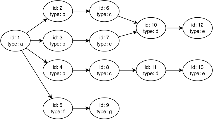
Figure 1: Example of an order received by our partner company.

This description of the order-to-cash process exhibits the causal structure in terms of which event triggers which subsequent event. Let us assume for the moment that we do not have any prior knowledge about causalities. Given is an event log of the process containing the following sequence recording only a fraction of the event types: $\langle a,c,f\rangle$. The observation of this single sequence does not allow us to conclude about the causal structure between the event types except that succeeding events cannot cause an event that had already happened earlier. That means, the evidence equally supports ($a$) causing ($c$) and ($c$) causing ($f$) as much as ($a$) causing ($c$) and ($a$) causing ($f$) or ($a$) and ($c$) combined causing ($f$). This observation does not change if we observe the same sequence ten times, one thousand times or more often. Indeed, in case of our industry partner, the invoicing is triggered by the completion of picking. However, due to typical delays of processing, the invoice is only emitted on the next business day when the delivery to the customer is already done. It should be noted that miners that use directly-follows relations are assuming causality from this sequence of execution.

The problem worsens if we consider cases with multiple instantiation. Problems of case identification and focus shifts have been described earlier [8, 20]. These problems stem from bundling and unbundling operations. Consider that picking is done in two steps: If an order event ($a$) leads to the creation of three order items ($b$) and their picking from the warehouse ($c$), we might observe an event sequence like $\langle a,b,c,b,b,c,c\rangle$. Clearly, ($b$) does neither cause itself nor is it caused by ($c$), but it results from the initial order with several items. Miners that use directly-follows relations cannot distinguish this situation where ($a$) causes several ($b$) events which each trigger a ($c$) from processes where a failures of ($b$) and ($c$) might cause repetitions.

The consequence of the described discovery problem is that directly-follows-based miners produce relationships that are not causal. For the case with $\langle a,c,f\rangle$, we obtain a relationship representing the wrong causality; for $\langle a,b,c,b,b,c,c\rangle$ even several wrong ones. In fact, only a subset of the directly-follows relationships are causal: Those from ($a$) to ($b$) and from ($b$) to ($c$). Notably, PM techniques based on directly-follows relations produce relationships that are spurious for the described process (from ($b$) to ($b$), from ($c$) to ($b$), and from ($c$) to ($c$)). Partially, these relationships are responsible for the commonly known Spaghetti model problem. Additionally, what is inextricably linked to the problem of spurious relationships is the misleading calculation of performance information related to time and cost. For instance, this leads to incorrect throughput times between two activities [17]. The question is how we can prevent these spurious relationships from being included in the output of the process miner?

The answer to this question is dissatisfactory for directly-follows miners and given by Pearl in the context of statistical inference [16, p. 59]: “Associations alone cannot identify the mechanisms responsible for the changes that occurred, the reason being that surface changes in observed associations do not uniquely identify the underlying mechanism responsible for the change.” This observation also holds for PM: If miner $X$ constructs model $x$ and miner $Y$ model $y$ both with 100% fitness, the event data offers no evidence to refute any of these models even if the one with higher precision might look more plausible. Connected to this, another problem occurs which is often denounced by analysts who use these models for process improvement and root-cause analysis: Having models with a high fitness helps to get a realistic picture of the process in a holistic manner. Nevertheless, common miners require input that flattens the process instance relation and maps it to a single case identifier, which in turn inflates the directly-follows graph as an output. What is missing are techniques that avoid spurious relationships, misleading connections, or inaccurate proportions right from the start.

Pearl describes a way out of this dilemma by the help of his three-level causal hierarchy [16]. The levels are distinguished by the queries that they are able to answer. The 1 level refers to associations and queries like “what is associated with each other?”. Queries at this level can be fully answered based on observations. The 2 level refers to interventions and queries like “what will happen if we intervene?”. Already at this level it cannot be fully answered based on observational data because it requires understanding of correlations. Level 3 refers to counterfactuals and queries like “what would have happened if we had not intervened?”. Queries at this level require knowledge of the functional mechanisms that produce observational data. Pearl describes that the limitations of the 1 level can be overcome by combining data with assumptions encoded in a causal model [16]. In this paper, we will transfer this idea formulated for statistical inference to our approach of CPM.

2.2 Requirements

To address the aforementioned challenges, we identify the following requirements.

RQ1: Input Data representing Causal Event Structure

The requirement is concerned with the input data for a PM algorithm. Instead of working with event logs defined for a single case notion, we observe the requirement to keep and represent the causality between events as stored in the source database. State-of-the-art techniques assume that this causal structure is unknown and typical try to reconstruct causality based on the directly-follows relations observed in the event log [1]. If the input for a PM technique already captures causal structures, this will avoid generating process models that include connection that are actually not causal.

RQ2: External Knowledge about Causal Event Structure

Based on Pearl’s comments, we observe the requirement to integrate domain knowledge about the causality between events into PM techniques. This is specifically needed to capture events and their causal relationships that can not be observed solely from the event data. Integrating this domain knowledge about causality facilitates the comparison with input data. In this way, input data can be validated and violations that contradict the causal structure can be identified.

RQ3: Event Cardinalities

We also observe the requirement to explicitly capture the cardinality between events and event types. The analysis of the cardinality is a key requirement for those processes that exhibit bundling and unbundling scenarios [8, 20], processes with divergence and convergence [10], or batching operations [21]. The lack of support by classic PM techniques leads to the construction of loops and spurious relationships for event types that are in a 1:N relationship with the event type that triggers a process.

RQ4: Aggregation of Causal Event Structures

We observe that PM techniques are required for constructing aggregated models from input based on causal event structures. A corresponding PM technique has to construct representations that support the analysis at a coarse-granular level of a process model as well as at the detailed level of a process instance. To this end, different business objects have to be selected as a focus of analysis. This would allow an analyst to inspect a business process at different levels of abstraction [22].

2.3 Prior Research

Next, we provide an overview of related work. We specifically focus on the extent to which existing approaches address or implement the four requirements we identified. We classify prior research that addressed the problem of causal relations and cardinality between events when learning a process model in two streams of research: (i) process discovery from relational databases where the causal relation and the cardinality are provided by the data structure; and (ii) approaches that infer the casual relation and cardinality information from flat event logs and then discover the process model.

For what concerns stream i), Li et al. [11] create an object-centric event log format, named eXtensible Object-Centric (XOC), that does not require a case notion as required for the XES format. Li et al. [11] argue that this object-oriented event log format helps to store relationships in the form of 1:N and N:M as it is common in databases. The problems of classic flattened event logs are also discussed in [10] in which an object-centric PM approach is presented. A projection of this event log considering the different existing objects allows for the discovery of the corresponding process model. In [23], an approach for discovering object-centric petri nets is presented. Moreover, Li et al. [24] suggest a method for identifying correlation between events considering the path between objects.

Pursuing a slightly different direction, Fahland [25] presents formal semantics for processes with N:M interactions considering unbounded dynamic synchronization of transitions, cardinality constraints, and history-based correlation of token identities. In [26] and [15], the cardinality is captured by the concept of one event being part of multiple cases by using labeled property graphs. Esser and Fahland [15, 26] transform event logs into graphs to store structural and temporal relationships between events. They discuss how edges between events define a causal relationship, based on the assumption that events are related to each other if there is an underlying entity to which both events belong. They later extend labeled property graphs to event knowledge graphs by integrating “further knowledge” like entity inference, resources, or actors [27, p. 285ff].

Berti and van der Aalst [13] propose an approach for learning models that represent multiple viewpoints of an event log stored in a relational database. These models are annotated with frequency and performance measures supporting the analysis of bottlenecks without the notion of a case. From these models, it is possible to derive event logs and reconstruct process models using standard PM tools. In [28], process cube operations such as slice and dice are applied to object-centric event logs for deriving object-centric sublogs. Furthermore, Lu et al. [9] generate a process model for each artifact out of event data extracted from a relational database. The foreign-key relationships are used to grasp causal dependencies between the events and define the order of the events in the event log. However, when discovery techniques are applied to the standard event log generated, the causal relation is not explicit and therefore not considered for the process model generation. A relation between the process models associated to the artifacts is discovered based on the cardinalities observed in the relational database. In this way, they are able to identify Artifact Type Level Interaction and Artifact Instance Level Interaction.

Table 1 summarizes how each of these prior works of stream i) meets the four requirements we identified above. ($\bullet$) indicates partial support.

Table 1: Specification of how the current approaches address the requirements of stream i)

Approach	RQ1	RQ2	RQ3	RQ4
van der Aalst and Berti [23]	$\bullet$		$\bullet$
van der Aalst [10]	$\bullet$		$\bullet$
Berti and van der Aalst [13]	$\bullet$		$\bullet$
Lu et al. [9]	$\bullet$		$\bullet$
Ghahfarokhi et al. [28]	$\bullet$			$\bullet$
Li et al. [11]	$\bullet$		$\bullet$
Li et al. [24]	$\bullet$	($\bullet$)	$\bullet$
Fahland [25]	$\bullet$		$\bullet$
Esser and Fahland [26]	$\bullet$		$\bullet$	$\bullet$
Esser and Fahland [15]	$\bullet$		$\bullet$	$\bullet$
Fahland [27]	$\bullet$	($\bullet$)	$\bullet$	$\bullet$

For what concerns stream ii), Song et al. [29] identify dependencies between activities based on control or data flow for discovery. A dynamic dependence graph captures all activities of the event log as well as their dependencies. The process model is then derived from this graph. In [30], techniques for identifying causality in the event log and filtering are used to learn instance graphs. Lu et al. [31] identify causality between events by modeling the traces as a partial order of its events [32]. The approach then uncovers patterns describing directly-cause, eventually-cause, and concurrence relations between events. The concurrence relation is defined by pairs of events that are not eventually-causing one another. Dumas and García-Bañuelos [33] discuss a PM approach based on Prime Event Structures (PESs). Their approach transforms the cases in an event log into PESs and then use the concept of asymmetric event structures to create a process model.

Ponce de León et al. use a similar approach [34] that creates labeled partial orders from the event log and independence information about the activities, merge them in an event structure, which is then transformed into an occurrence net. A process model is derived from folding the occurrence net. Furthermore, Bergenthum [35] also uses PESs as an intermediate step to create a process model. The approach learns concurrency between events and use it for deriving a partial order of the event log to yield its PES. Approaches by Weber et al. [22] and by Conforti et al. [36] present ideas that identify and hide subordinate processing paths and integrate them into multiple instance activities in the discovered models.

Table 2: Specification of how the current approaches address the requirements of stream ii)

Approach	RQ1	RQ2	RQ3	RQ4
Song et al. [29]	$\bullet$
Diamantini et al. [30]	$\bullet$
Dumas and García-Bañuelos [33]	$\bullet$			$\bullet$
Lu et al. [31]	$\bullet$
Ponce-de León et al. [34]	$\bullet$			$\bullet$
Bergenthum [35]	$\bullet$			$\bullet$
Weber et al. [22]	$\bullet$		$\bullet$	$\bullet$
Conforti et al. [36]				$\bullet$

Table 2 summarizes how each of these prior work of stream ii) meets the requirements we defined in Section 2.2.

Almost all these works have in common that they make a best effort for reconstructing the causal relationships between the events and activities of the underlying multi-perspective business process. Nevertheless, as Pearl emphasizes, the level of intervention and counterfactual queries is not reachable for those purely data-driven approaches since they only contain “purely observational information” [16, p. 56]. We address this problem in the next section by developing a CPM approach that we call Noreja, which is based on Causal Event Graphs (CEGs) and Aggregated Causal Event Graphs (ACEGs). We use a CPT to internalize external knowledge based on causal assumptions of domain experts as as well as meta information from relational databases (e.g., cardinalities like 1:N and N:M) [16].

3 An Approach to Causal Process Mining

In this section, we introduce our CPM approach and explain how it differentiates itself from classical approaches. Then, we summarize preliminaries from prior research, provide definitions of the key formal notions, define formal operations, and describe visualizations.

3.1 Setting the Broader Context

Before going into the details of our approach, we want to juxtapose it with classical PM approaches based on DFGs and event logs. Figure 2 gives an overview of the different steps of each approach and where humans are involved. Classical approaches (top lane in Figure 2) build on four steps. First, transactions are inserted into a database during the execution of a business process. Those transactions are persisted inside tables of relational databases, which themselves are connected by foreign-key relations with different cardinalities. Second, in preparation for creating the event log, a process expert defines the obligatory case identifier, specifies the process activities and related properties, such as resources, timestamps, or other business objects. Based on this information, a flattened event log is extracted. Third, the event log is loaded into memory where the DFG is calculated as an output. Fourth, a process analyst can interpret the visualization on the screen.

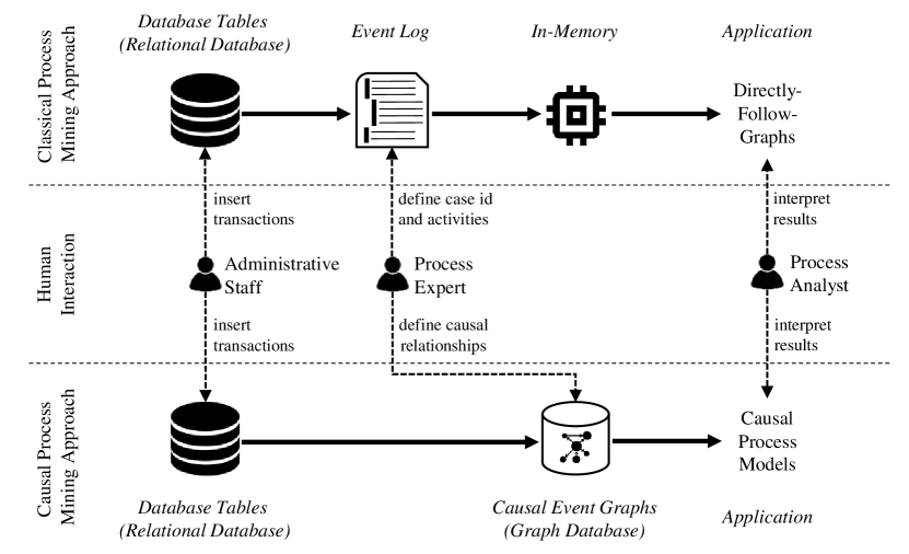
Figure 2: Differences between causal and classical (event log based) PM

Our CPM approach (bottom lane in Figure 2) extracts the relevant data from a relational database, which matches the classical approach. However, the second step has fundamental differences, because the extraction of a dedicated event log is skipped. Instead, we directly transfer the relational database structures into CEGs and store them in a graph database. In this way, we avoid flattening the data, such that we keep cardinalities and causal relationships between data objects. The user-facing application then only has to visualize the CEGs in a use-case specific manner. From a technical perspective, this shifts computation from the application layer to the database layer. We obtain reusability as different user-facing applications can query the data independently, and flexibility as the CEG is not bound to a predefined case identifier. In the subsequent sections, we present our approach from formal perspective.

3.2 Noreja Approach

The Noreja Approach for Causal Process Mining (CPM)consists of the following consecutive steps: (i) First, a set of relevant tables is selected from the source relational database and joined over foreign keys. (ii) Then, the Causal Process Template (CPT)is defined. (iii) Afterwards, each causally connected tuple in the joined tables is transformed to a so-called Causal Event Graph (CEG)by merging fragments that share common events. (iv) Based on the CEG, different aggregations, called ACEG, are calculated for each primary key. (v) Eventually, the CEGs and the ACEGs are used to analyze the processes. Next, we discuss each step in turn.

3.2.1 Input Data Selection

The first step of the Noreja Approach is concerned with determining which tables of a relational database are required for analysis. To this end, we recall the definition of a database schema based on Calvanese et al [37].

Definition 1 (Relational Schema)

Let $R$ be the set of relations of a relation database. A relational schema of a relation $r\in R$ is a pair $\langle r.name,r.attrs\rangle$, where $r.name$ is the relation name and $r.attrs$ is a nonempty tuple of attributes. The first attribute in $r.attrs$ must be the identifier denoting the primary key ($r.pk$) followed by identifiers of other relations denoting foreign keys ($r.FK=\{r.fk_{1},...,r.fk_{n}\}$), when existing, a time ($r.timestamp$) registering a time event, and lastly other attributes. We call $|r.attrs|$ the arity of $r$.

Definition 2 (Catalog)

Let $R$ be the set of relations of a relation database. A catalog $Cat$ is any subset of relations ($Cat\subseteq R$) where every two relations $r_{i},r_{j}\in Cat$ have different primary keys ($r.pk_{i}\neq r.pk_{j}$) in their relational schemas.

A catalog of relations $Cat$ may be selected by a process analyst and its relations joined using the left outer join $\bowtie_{L}$.

Definition 3 (Left Outer Join, Causally Connected Tuple)

Let $Cat=\{r_{1},\dots,r_{n}\}$ be a catalog. Left outer join is a relational schema $r_{J}=r_{1}\bowtie_{L}r_{2}\dots r_{n-1}\bowtie_{L}r_{n}$ such that for each $r_{i}\in Cat$, there exists another $r_{j}\in Cat$ with $j\neq i$, such that either $\exists r_{j}.fk\in r_{j}.FK$ where $r_{j}.fk=r_{i}.pk$ or $\exists r_{i}.fk\in r_{i}.FK$ where $r_{i}.fk=r_{j}.pk$. We call a row in $r_{J}$ a causally connected tuple.

As an example, Figure 3 depicts an ER-diagram of a catalog from an order-to-cash process, $Cat=\{$ $Purchase\,Orders,$ $Order\,Items,$ $Shipments,$ $Customer\,Pickups\}$.

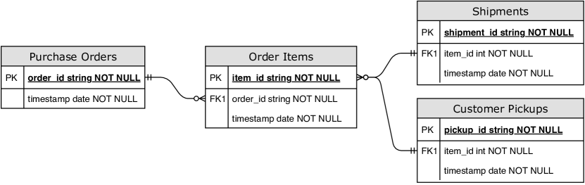
Figure 3: Example ER-diagram. Note: To simplify the diagram, we have omitted additional properties, e.g., customer name, item type, shipment address, etc.

The Purchase Orders table holds the order received events, i.e., an event is persisted in the table as soon as an order is received. The order is then broken down into a list of items, which are then separately picked from the warehouse. These warehouse picking events are stored in Order Items. As can be seen in the ER-Diagram, each of these Order Items is linked to a Purchase Order via a foreign-key relationship. Eventually, the items are shipped to the customer, these events are stored in the Shipments table, or directly picked up by the customer, these events are stored in the Customer Pickups table. Again these events are related to the corresponding Order Items via foreign-key relationships. We can define the left outer join $r_{J}$ over these tables using the foreign-key relationships. A causally connected tuple contains, for instance, one order_id indicating the purchase order, one item_id indicating a corresponding order item, and either the corresponding shipment_id or pickup_id. Mind that if identifiers in connected tables do not exist, the left outer join will include $null$ values.

3.2.2 Causal Process Template Definition

The left outer join over the selected tables has yielded a relation, in which each row is a causally connected tuple. Our approach requires a process analyst to specify a partial order over the selected relations. We call such a partial order Causal Process Template (CPT).

Definition 4 (Causal Process Template)

Let $Cat=\{r_{1},\dots,r_{n}\}$ be a catalog. A Causal Process Template (CPT)is a partial order $\prec~{}\subseteq Cat\times Cat$ over the relations of the catalog.

The CPT is the basis for constructing the causal relationships over the activities of a process. It can be defined based on the ER-diagram or on an adaptation of it. In our example, a customized CPT could define that the Customer Pickups is a causal successor of Purchase Orders and not of Order Items as it is defined in the ER-Diagram. After the catalog and the CPT are defined, the Causal Event Graph (CEG)is constructed.

3.2.3 Causal Event Graph Construction

A Causal Event Graph (CEG)provides the means to model events and the causal relationship between them. An event and a CEG are defined as follows.

Definition 5 (Event)

Let $Cat=\{r_{1},\dots,r_{n}\}$ be a catalog. An event $e_{i}^{v}$ of a relation $r_{i}\in Cat$ is a tuple $e_{i}^{v}=<r_{i}.pk^{v},r_{i}.timestamp^{v}>$ which indicates the value of the attributes $r_{i}.pk$ and $r_{i}.timestamp$, i.e., which is the identifier of the event and when it happened. An event $e_{i}^{v}$ is associated with a tuple of the table $r_{i}$.

Definition 6 (Causal Event Graph)

Let $Cat=\{r_{1},\dots,r_{n}\}$ be a catalog, $\prec\subseteq Cat\times Cat$ the CPT over $Cat$, $r_{J}=r_{1}\bowtie_{L}r_{2}\dots r_{n-1}\bowtie_{L}r_{n}$ the left outer join of the relations in $Cat$ considering the defined CPT, and $rj$ a causally connected tuple of $r_{J}$. A Causal Event Graph is a tuple $CEG=\langle E,\leq,\lambda\rangle$, where $E\subseteq\{e_{1}^{{rj}_{1}},\dots,e_{1}^{{rj}_{n}},\dots,e_{n}^{{rj}_{1}},\dots,e_{n}^{{rj}_{n}}\}$, $\leq~{}\subseteq E\times E$ is a binary relation where $(e_{i}^{rj},e_{j}^{rj})\in\leq$ if $r_{i}\prec r_{j}$, and $\lambda:E\to ET$ is the labeling function that defines the event type of an event.

For each causally connected tuple $rj$ of $r_{J}$, a CEG ($CEG_{rj}$) may be created where $E$ is the set of events associated with the tuple $rj$. The set $r_{J}$ of all causally connected tuples $rj$ of a relational database catalog $Cat$ induces the Causal Event Database $CEG_{DB}=\bigcup_{rj\in r_{J}}CEG_{rj}$. For that a $CEG_{rj}$ is called a fragment of $CEG_{DB}$. Two or more fragments may have common events, for instance, when two orders share one delivery. In this case, the fragments are connected and the shared event is called a batching event [21]. Overall, $CEG_{DB}$ is typically disconnected and the maximally connected components define a partition of $CEG_{DB}$. Accordingly, we define two functions:

• $Comp(CEG_{DB})$: it returns the set of all components of $CEG_{DB}$, and

• $Frag(CEG_{DB})$: it returns the set of all fragments $CEG_{rj}$ of $CEG_{DB}$ where $rj\in r_{J}$.

As an example, Figure 4 shows an instantiation of the relational database defined in Figure 3. According to the Noreja Approach, we construct the following CEGs fragments (Figure 5 depicts them graphically). For simplification, we used the identifier value as the label of the events.

• $CEG_{1}=\langle E_{1},\leq_{1},\lambda_{1}\rangle$ with

  • $E_{1}=\{or1,pi1,pi2,pi3,sh1,sh2\}$,

  • $\leq_{1}=\{(or1,pi1)$, $(or1,pi2)$, $(or1,pi3)$, $(pi1,sh1)$, $(pi2,sh1)$,
    $(pi3,sh2)\}$, and

  • $\lambda_{1}=\{(or1,Receive\;Purchase\;Order)$, $(pi1,Pick\;Order\;Item)$,
    $(pi2,Pick\;Order\;Item)$, $(pi3,Pick\;Order\;Item)$,
    $(sh1,Register\;Shipment)$, $(sh2,Register\;Shipment)\}$

• $CEG_{2}=\langle E_{2},\leq_{2},\lambda_{2}\rangle$ with

  • $E_{2}=\{or2,pi4,sh2\}$,

  • $\leq_{2}=\{(or2,pi4)$, $(pi4,sh2)\}$, and

  • $\lambda_{2}=\{(or2,Receive\;Purchase\;Order)$, $(pi4,Pick\;Order\;Item)$,
    $(sh2,Register\;Shipment)\}$

• $CEG_{3}=\langle E_{3},\leq_{3},\lambda_{3}\rangle$ with

  • $E_{3}=\{or3,pi5,cu1\}$,

  • $\leq_{3}=\{(or3,pi5)$, $(pi5,cu1)\}$, and

  • $\lambda_{3}=\{(or3,Receive\;Purchase\;Order)$, $(pi5,Pick\;Order\;Item)$,
    $(cu1,Register\;Customer\;Pickup)\}$

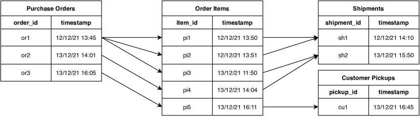
Figure 4: Example instantiation of the database. The arrows depict the relationships between the entries.

((a)) CEG of Purchase Order or1.

((b)) CEG of Purchase Order or2.

((c)) CEG of Purchase Order or3.

Figure 5: CEGs fragments for the data shown in Figure 4.

Furthermore, we define the following accompanying functions and concepts.

Definition 7 (Preset and Postset Nodes)

Let $E$ be a set of events, and $R\subseteq E\times E$ a binary relation over $E$. We define the preset function ${\bullet\,{e}}:E\rightarrow\mathcal{P}(E)$ as ${\bullet\,{e}}=\{x\in E~{}|~{}(x,e)\in R\}$ for an event $e\in E$. As well as the postset function ${e}\bullet:E\rightarrow\mathcal{P}(E)$ as ${e}\bullet=\{x\in E~{}|~{}(e,x)\in R\}$ for an event $e\in E$.

Definition 8 (Event Type, Identifier and Time)

Let $E$ be a set of events, and $ET$ the set of event types. We define $\tau:E\to ET$ as the function that returns the event type of an event $e\in E$. We define $e^{\tau}=\tau(e)$. We define $\mathrm{id}:E\to I$ as an index function and $\mathrm{t}:E\to\mathbb{R}$ as a time function.

The result of this construction are CEGs that are partially disconnected. However, fragments are partially connected via batching events e.g., the shipment event sh2 is shared between the order received event or1 and or2.

To find all batching events of a given CEG for analysis purposes, we define the following function.

Definition 9 (Batching Event)

Let $E$ be a set of events. We define a function $\mathrm{batch}:E\to\mathbb{N}$ that returns $1$ when an event is a batch event and $0$ otherwise.

We also define the following function that returns the cycle time between a given event and its causal predecessors.

Definition 10 (Event Cycle Time)

Let $E$ be a set of events. For each event $e\in E$, we define its cycle time as a function $cyc:E\to\mathbb{N}$ such that
$cyc(e)=\begin{cases}t(e)-\max(\{t(x)|x\in{\bullet\,{e}}\wedge t(x)\leq t(e)\}),&\text{if }{\bullet\,{e}}\neq\emptyset\wedge\exists x\in{\bullet\,{(}}e)|t(x)\leq t(e)\\ 0,&\text{otherwise}\end{cases}$

As defined in Definition 10, the cycle time of an event $e$ is the timespan between the event and the latest precedent event, i.e., $\max(t({\bullet\,{e}}))$. Mind that this calculation includes both waiting time and processing time. Also, if the event $e$ is a start event, i.e., ${\bullet\,{e}}=\emptyset$, there is no precedent event. In such situations, different customized options are possible e.g., a 0 or a NULL value could be returned. Another option is to use estimations like those proposed in [38].

3.2.4 Causal Event Graph Aggregation

In the next step of the Noreja Approach, different aggregation levels of the transformed CEGs are created. Before we discuss the different aggregation levels, we have to define how an aggregation of a CEG is created.

As a first step, a set of event types $ET$ is created from all types $e^{\tau}$ of all events $e\in E$ of the CEG. For instance, when we consider $CEG_{1}$ from Section 3.2.3 (depicted in Figure 5(a)) and that the labels $\lambda_{1}$ define the event types, then the final set of aggregated event types $ET$ contains Receive Purchase Order, Pick Order Item, and Register Shipment.

For the aggregation of the CEG, we have to calculate the quantity for each event type with the help of the function $c(E,et)$.

Definition 11 (Event Type Quantity)

Let $E$ be a set of events, $ET$ a set of event types, and $et\in ET$ an event type. We define the event type count $c:\wp(E)\times ET\to\mathbb{N}$ such that $c(X,et)=|\{e\in X~{}|~{}e^{\tau}=et\}|$, where $X\subseteq\wp(E)$.

For instance, for $CEG_{1}$ the resulting quantities for aggregated event types $et\in ET$ are:

• $c(E_{1},Receive\;Purchase\;Order)=1$,

• $c(E_{1},Pick\;Order\;Item)=3$, and

• $c(E_{1},Register\;Shipment)=2$.

As a next step, we add a causal relationship between two event types, $et_{a},et_{b}\in ET$, iff there exist two events, $e_{a},e_{b}\in E$, in the CEG such that $et_{a}=\tau(e_{a})$, $et_{b}=\tau(e_{b})$, and $(e_{a},e_{b})\in\leq$ in the CEG. For instance, for $CEG_{1}$ this would be the case for the event types Receive Purchase Order and Pick Order Item, and Pick Order Item and Register Shipment.

Also for the aggregated relationships the quantities are calculated. This is done via the function $cr(R,et_{1},et_{2})$ defined in Definition 12.

Definition 12 (Event Type Relationship Quantity)

Let $E$ be a set of events, $R\subseteq E\times E$ a binary relation over $E$, $ET$ a set of event types, and $et_{1},et_{2}\in ET$ event types. We define the quantity of the relationship between event types $cr:R\times ET\times ET\to\mathbb{N}$ such that $cr(R,et_{1},et_{2})=|\{v\in E~{}|~{}(v,w)\in R,v^{t}=et_{1},w^{t}=et_{2}\}|$

For $CEG_{1}$ (cf. Figure 5(a)) the following relationship quantities are calculated:

• $cr(\leq,Receive\;Purchase\;Order,Pick\;Order\;Item)=1$,

• $cr(\leq,Pick\;Order\;Item,Register\;Shipment)=3$.

As a last step, the outgoing and incoming cardinalities of each relationship are calculated. For this, we first define the functions $\mathrm{Out}(v,et,R)$ (Definition 13) and $\mathrm{In}(v,et,R)$ (Definition 14).

Definition 13 (Event to Event Type Outgoing Cardinality)

Let $E$ be a set of events, $R\subseteq E\times E$ a binary relation over $E$, and $ET$ a set of event types. We define the number of outgoing relationships of an event $v\in E$ to an event type $et\in ET$ as $\mathrm{Out}:E\times ET\times\wp(R)\to\mathbb{N}$ such that $\mathrm{Out}(v,et,R)=|\{(v,w)\in R~{}|~{}w^{t}=et\}|$.

This means that the function $\mathrm{Out}(v,et,R)$ calculates the output degree of an event $e\in E$ to a particular event type $et\in ET$. For instance, for $CEG_{1}$ the resulting output degrees are:

• $\mathrm{Out}(or1,\text{\emph{Pick Order Item}},\leq_{1})=3$ and

• $\mathrm{Out}(pi3,Register\;Shipment,\leq_{1})=1$.

Definition 14 (Event to Event Type Incoming Cardinality)

Let $E$ be a set of events, $R\subseteq E\times E$ a binary relation over $E$, and $ET$ a set of event types. We define the number of incoming relationships to an event type $et\in ET$ from an event $v\in E$ as $\mathrm{In}:ET\times E\times\wp(R)\to\mathbb{N}$ such that $\mathrm{In}(et,v,R)=|\{(v,w)\in R~{}|w^{t}=et\}|$.

By this definition, the function $\mathrm{In}(et,v,R)$ calculates the input degree from an event type $e^{t}$ to an event $e\in E$. In $CEG_{1}$ the resulting cardinalities are:

• $\mathrm{In}(\text{\emph{Pick Order Item}},or1,\leq_{1})=1$ and

• $\mathrm{In}(Register\;Shipment,pi3,\leq_{1})=1$.

To be able to describe the cardinality between two event types, we have to extend the functions from Definition 13 and Definition 14 with the possibility to get the minimum and maximum of $\mathrm{Out}(v,et,R)$ and $\mathrm{In}(et,v,R)$. To this end, we first define the functions to calculate the minimum and maximum for the outgoing cardinality, Definition 15, and then the functions to calculate the same for the incoming cardinality in Definition 16.

Definition 15 (Minimum and Maximum Outgoing Cardinality)

Let $E$ be a set of events, $R\subseteq E\times E$ a binary relation over $E$, $ET$ a set of event types, and $et_{1},et_{2}\in ET$ event types. We define

• the minimum outgoing cardinality from one event type to another event type as $\mathrm{MinOut}:\wp(R)\times ET\times ET\to\mathbb{N}$ such that $\mathrm{MinOut}(R,et_{1},et_{2})=\min(\{out(v,et_{2},R)~{}|~{}v\in E\wedge v^{t}=et_{1}\})$, and

• the maximum outgoing cardinality from one event type to another event type as $\mathrm{MaxOut}:\wp(R)\times ET\times ET\to\mathbb{N}$ such that $\mathrm{MaxOut}(R,et_{1},et_{2})=\max(\{out(v,et_{2},R)~{}|~{}v\in E\wedge v^{t}=et_{1}\})$.

When we apply these functions $MinOut$ and $MaxOut$ to $CEG_{1}$, we get the following results for the relationship:

• between Receive Purchase Order and Pick Order Item
  $MinOut(\leq_{1},Receive\;Purchase\;Order,Pick\;Order$ $Item)=3$ and
  $MaxOut(\leq_{1},Receive\;Purchase\;Order,Pick\;Order\;Item)=3$ , and

• between Pick Order Item and Register Shipment
  $MinOut(\leq_{1},Pick\;Order\;Item,Register\;Shipment)=1$ and
  $MaxOut(\leq_{1},Pick\;Order\;Item,Register\;Shipment)=1$ .

Definition 16 (Minimum and Maximum Incoming Cardinality)

Let $E$ be a set of events, $R\subseteq E\times E$ a binary relation over $E$, $ET$ a set of event types, and $et_{1},et_{2}\in ET$ event types. We define

• the minimum incoming cardinality from one event type to another
  event type as $\mathrm{MinIn}:\wp(R)\times ET\times ET\to\mathbb{N}$ such that $\mathrm{MinIn}(R,et_{1},et_{2})=\min(\{in(et_{1},v,R)~{}|~{}v\in E\wedge v^{t}=et_{2}\})$, and

• the maximum incoming cardinality from one event type to another event type as $\mathrm{MaxIn}:\wp(R)\times ET\times ET\to\mathbb{N}$ such that $\mathrm{MaxIn}(R,et_{1},et_{2})=\max(\{in(et_{1},v,R)~{}|~{}v\in E\wedge v^{t}=et_{2}\})$.

By apply the functions $MinIn$ and $MaxIn$ to $CEG_{1}$ we get the following resulting cardinalities:

• $MinIn(\leq_{1},Pick\;Order$ $Item,Receive\;Purchase\;Order)=1$ and

• $MaxIn(\leq_{1},Pick\;Order\;Item,Receive\;Purchase\;Order)=1$, and

• $MinIn(\leq_{1},Register\;Shipment,Pick\;Order\;Item)=1$ and

• $MaxIn(\leq_{1},Register\;Shipment,Pick\;Order\;Item)=2$.

Summarizing, we define an aggregation of a CEG, called a ACEG, the following way:

Definition 17 (Aggregated Causal Event Graph)

A tuple $ACEG=\langle ET,\leq,\circ,\bowtie,\rtimes,\ltimes,\lambda\rangle$ is a labeled Aggregated Causal Event Graph (ACEG), where $ET$ is a set of event types, $\leq$ is the causality binary relation on $ET$, $\circ:ET\to\mathbb{N}$ defines the quantity of the events of a event type, $\bowtie:\leq\to\mathbb{N}$ defines the quantity of the causality relations, $\rtimes:\leq\to\mathbb{N}\times\mathbb{N}$ defines the minimum and maximum incoming cardinality of the causality relations, $\ltimes:\leq\to\mathbb{N}\times\mathbb{N}$ defines the minimum and maximum outgoing cardinality of the causality relations, and $\lambda:ET\to\Lambda$ is the labeling function, such that $\leq$ is a partial order.

As an example, the formal specification of the ACEG of $ceg_{1}$ is defined by $ACEG_{1}=\langle ET,\leq,\circ,\bowtie,\rtimes,\ltimes,\lambda\rangle$ with

• $ET=\{or,pi,sh\}$,

• $\leq=\{(or,pi)$, $(pi,sh)\}$,

• $\circ=\{(or,1)$, $(pi,3)$, $(sh,2)\}$,

• $\bowtie=\{(or,pi,1)$, $(pi,sh,3)\}$,

• $\rtimes=\{(or,pi,1,1)$, $(pi,sh,1,2)\}$,

• $\ltimes=\{(or,pi,3,3)$, $(pi,sh,1,1)\}$, and

• $\lambda=\{(or,Receive\;Purchase\;Order)$, $(pi,Pick\;Order\;Item)$,
  $(sh,Register\;Shipment)\}$

Figure 6 depicts the resulting ACEG graphically.

Figure 6: Aggregation of of $CEG_{1}$, from Section 3.2.3. Node and relationship quantity in parenthesis and relationship cardinality in the form {$\rtimes_{min}$..$\rtimes_{max}$ : $\ltimes_{min}$..$\ltimes_{max}$}.

In the figure, the node and relationship quantities, i.e., $\circ$ and $\bowtie$, are shown in parenthesis. For simplification, the cardinality functions, i.e., $\rtimes$ and $\ltimes$, are represented in the format {$\rtimes_{min}$..$\rtimes_{max}$ : $\ltimes_{min}$..$\ltimes_{max}$} in which the first pair of elements, i.e., $\rtimes_{min}$..$\rtimes_{max}$, represent the minimum and maximum of the incoming cardinality and the second pair, i.e., $\ltimes_{min}$..$\ltimes_{max}$, the minimum and maximum of the outgoing cardinality.

The Noreja Approach provides three different levels of aggregation, which allows the analysis of the process on three different levels of detail:

Aggregation Level 1

The 1 aggregation level creates an ACEG for each CEG. As a result, the amount of ACEGs is equal to the amount of CEGs. In comparison to the detailed level that the CEGs provides, the 1 aggregation level provides a lower level of detail but allows a more general analysis of the executed process instances. As an example, Figure 7 depicts the constructed ACEGs from the CEG depicted in Figure 5.

((a)) ACEG of $CEG_{1}$.

((b)) ACEG of $CEG_{2}$.

((c)) ACEG of $CEG_{3}$.

Figure 7: 1 aggregation level of the CEG depicted in Figure 5.

Aggregation Level 2

The 2 aggregation level creates an ACEG for all CEGs that have the same structure. Two CEG have the same structure iff the event types $ET$, relationships $\leq$, and labels $\lambda$ of the corresponding ACEG, from the 1 aggregation level, are equal. As a result, the amount of ACEGs is lower or equal to the amount of CEGs. Again, this aggregation level decreases the level of detail in comparison to the 1 aggregation level but provides a higher view of the executed process instances. As an example, Figure 8 depicts the transformed ACEGs from the CEG depicted in Figure 5. As can be seen, $CEG_{1}$ and $CEG_{2}$ are aggregated to one ACEG since they have the same structure. $CEG_{3}$, on the other hand, has another structure, since the last event is a Register Customer Pickup event instead of a Register Shipment event.

((a)) Transformed ACEG of $ceg_{1}$ and $ceg_{2}$.

((b)) Transformed ACEG of $ceg_{3}$.

Figure 8: 2 aggregation level of the CEG depicted in Figure 5.

Aggregation Level 3

The 3 aggregation level creates one ACEG for the whole $CEG_{DB}$, i.e., all CEGs. Therefore, this aggregation level is the highest and provides a complete view of the executed process instances. For instance, Figure 9 depicts the transformed ACEGs from the CEG depicted in Figure 5.

Figure 9: 3 aggregation level of the CEG depicted in Figure 5.

These three aggregation levels together with the CEGs provide the means to analyze the process on the lower instance level as well as on different higher levels, with the process model at the highest level.

3.3 Causal Event Graph Analysis

In general, the analysis possibilities provided by the Noreja Approach can be categorized into Visualisation, Key Performance Indicators (KPIs), and Violations. We will discuss these categories and give some examples of how the analysis can be done using the Noreja Approach.

3.3.1 Visualisation

The first analysis category of visualisations presents the CEGs and ACEGs to the analyst. This provides the analyst with a way to visually inspect the processes on the different detail levels, i.e., from a detailed process instance level provided by the CEGs to a high process model level provided by the ACEGs. The CEGs and ACEGs can be shown to the analyst as graphs, similar as, e.g., Figure 5 for the CEG level or Figure 9 for the ACEG level. Moreover, by displaying the ACEGs from Aggregation Level 2, the analyst can analyze the different process variations as shown in Figure 8.

3.3.2 Key Performance Indicator

The second analysis category focuses on the representation of KPIs of the observed fragments. Different KPIs can be calculated, among them are, for instance:

• Minimum, Average, and Maximum Cycle Time of an Event Type: The calculation of this KPI is shown in Algorithm 1. The algorithm takes as input a set of CEGs and an event type. The algorithm, then iterates through the CEGs and calculates the minimum, average, and maximum event type cycle time of the requested event type.

• Minimum, Average, and Maximum CEG Cycle Time: The calculation of this KPI is shown in Algorithm 2. This algorithm takes as input a set of CEGs. The algorithm then iterates through the set of CEGs and searches for the event with the smallest timestamp, i.e., $min_{ceg}=\min(\{t(e)~{}|~{}e\in E_{ceg}\})$, and the event with the biggest timestamp, i.e., $max_{ceg}=\max(\{t(e)~{}|~{}e\in E_{ceg}\})$. The found $min_{ceg}$ and $max_{ceg}$ timestamps are then used to calculate the CEG cycle time which is added to a set of cycle time. Eventually, the collected cycle time are used to calculate the minimum, the average, and the maximum CEG cycle time.

• Minimum, Average, and Maximum Fragment Cycle Time: The calculation of this KPI is similar to the one for the CEG cycle time, but on a fragment level. Therefore, Algorithm 2 gets as input a set of fragments instead of a set of CEGs.

• Distribution End Event Types: This KPI shows the distribution of end event types of the observed paths. For this KPI, the 3 aggregation level ACEG is used. A set of all end event types, together with the corresponding quantity, is created as follows: $\mathbb{E}=\{et\in ET~{}|~{}{et}\bullet=\emptyset\}$. This set can then be used to calculate the absolute and relative distribution of end events.

• Batching Event Type Distribution: To calculate the distribution of batching event types, we first get a list of batching events by $\mathbb{B}=\{e\in E~{}|~{}batch(e)=1\}$. Afterwards the absolute and relative distribution can be calculated by using the event types of the batching events: $\mathbb{BT}=\{e^{\tau}~{}|~{}e\in\mathbb{B}\}$.

Algorithm 1 Get Minimum, Average, and Maximum Event Type Cycle Time

1:$C=\{CEG_{1},CEG_{2},...,CEG_{n}\};an\;event\;type\;et$

2:$min,avg,max$ event type cycle time

3:$cycleTime=\emptyset$

4:for all $CEG=\langle E,\leq,\lambda\rangle\in C$ do

5:     for all $e\in E$ do

6:         if $e^{\tau}=et$ then

7:              $cycleTime=cycleTime\cup\mathrm{cyc}(e)$;

8:         end if

9:     end for

10:end for

11:$min=min(cycleTime)$;

12:$max=max(cycleTime)$;

13:$avg=avg(cycleTime)$;

14:return $min,avg,max$;

Algorithm 2 Get Minimum, Average, and Maximum CEG cycle time

1:$C=\{CEG_{1},CEG_{2},...,CEG_{n}\}$

2:$min,avg,max$ fragment cycle time

3:$cycleTime=\emptyset$

4:for all $CEG=\langle E,\leq,\lambda\rangle\in C$ do

5:     $min_{CEG}=\min(\{t(e)~{}|~{}e\in E\})$;

6:     $max_{CEG}=\max(\{t(e)~{}|~{}e\in E\})$;

7:     $cycleTime_{CEG}=max_{CEG}-min_{CEG}$;

8:     $cycleTime=cycleTime\cup cycleTime_{CEG}$;

9:end for

10:$min=min(cycleTime)$;

11:$max=max(cycleTime)$;

12:$avg=avg(cycleTime)$;

13:return $min,avg,max$;

3.3.3 Violations

The third analysis category is about the analysis of violations. The focus here is the temporal order of events as observed in comparison to what is expected according to the CPT. Such temporal violations can be detected by comparing the timestamps between two events, $e_{a},e_{b}\in E$, for which there exists a causal relationship $e_{a}\leq e_{b}$. A causal relationship $e_{a}\leq e_{b}$ defines that an event $e_{a}$ causes an event $e_{b}$, as a consequence the timestamp $t(e_{a})$ should be before $t(e_{b})$. If this is not the case, the causal relationship is violated. With a given set of CEG, a set with all the pairs that violated the temporal order can be created as follows: $\mathbb{V}_{o}=\{(e_{a},e_{b})\in\leq|t(e_{a})<t(e_{b})$}.

4 Evaluation

In the following, we evaluate the Noreja Approach by comparing it to state-of-the-art process discovery algorithms. To this end, we first discuss the dataset that we use and our prototypical implementation. Then, we compare the solutions qualitatively and quantitatively.

4.1 Evaluation Case

We use a real-world dataset from our industry partner, an European food production company, which captures the events of the order-to-cash process. The process is triggered by supermarket orders (a). These orders are broken down into a list of item suborders (b). Each of these items is separately picked from the warehouse (c). Then commissioned (and packaged) (d) and sent as one or multiple deliveries (e). Finally, an invoice is sent to the customer (f). Some of these steps also contain substeps. Furthermore, each step of an order can also be batched together with another order, e.g., several orders might be batched in one delivery.

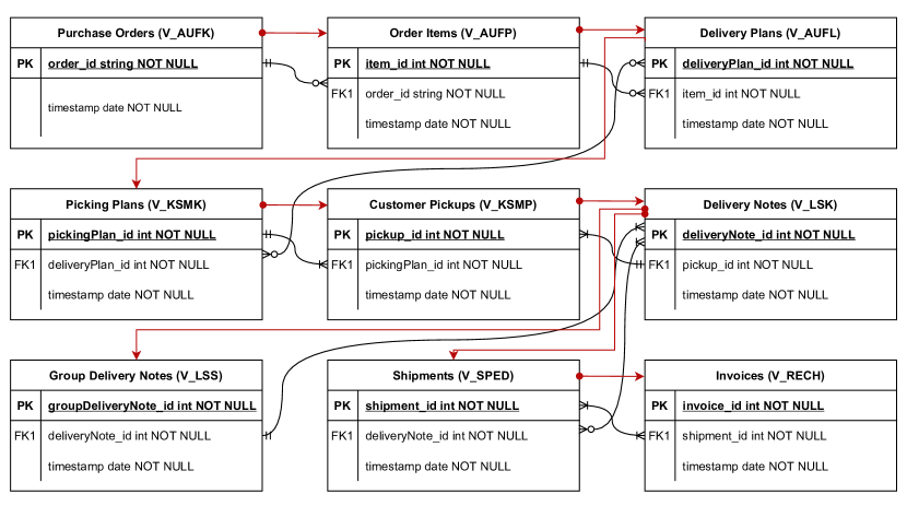
Figure 10: ER diagram of source data tables and CPT of the Order-to-Cash process (in red). Note: We link the following event labels to the tables: V_AUFK: Receive Order, V_AUFP: Extract Order Items, V_AUFL: Prepare Order Delivery, V_KSMK: Plan Order Item Picking, V_KSMP: Pick Order Item, V_LSK: Create Delivery Note, V_LSS: Generate Group Delivery Note, V_SPED: Deliver Order, V_RECH: Post Invoice.

The company uses an ERP system built on a Microsoft SQL Server, which serves as the data source for our evaluation. We used the following catalog of tables: $Cat=\{V\_AUFK,V\_AUFP,V\_AUFL,V\_KSMK,V\_KSMP,\\ V\_LSK,V\_LSS,V\_SPED,V\_RECH\}$. Figure 10 depicts the ER-diagram for $Cat$ and also shows the CPT describing the partial order assumed among the relations in $Cat$ (in red). This partial order was built based on the foreign key relations and the causal knowledge of the analyst. In total, the dataset contains 70,000 orders with more than 8,500,000 events.

For each event, the ERP system stores, besides different resource properties, the start timestamp that marks the start of an event, and the last update timestamp that marks the end of an event. For the evaluation, we use the raw event data without any data cleaning beforehand. Note that publicly available dataset of the BPI Challenges are flat event logs. As our approach leverages external knowledge about causal structures as available in a relational database, we could not use these public datasets.

4.2 Prototype

Our prototype is implemented as a component of the commercial Noreja tool as a Java microservice-based application, using Spring Boot (vers. 2.4.4), and a TypeScript based Angular (vers. 12.2.10) web user interface (UI). To store and query the CEGs and ACEGs, we use the graph database Neo4j (vers. 4.3.0) and Cypher as the Neo4j query language. The current prototype can read event data from Microsoft SQL Server and Oracle DB.

Figure 11 to Figure 13 present three screenshots of the UI. Figure 11 shows a single CEG, which was selected from the list of available CEGs on the left side. Events are visualized as blue rhombuses, called diamonds. Cyan-colored circles and triangles are used to mark the start and end of a process. A triangle marks a start or end of a path for which there is a parallel path that continous, e.g., the path at the bottom after Prepare Order Delivery in Figure 11, these triangle markers are called intermediate start or end. A circle marks the start or end of the process for which there is no parallel continuing path. Figure 12 shows the 1 aggregation level ACEG of the CEG shown in Figure 11. As discussed in Section 3.2.4, the relationship and node quantity are shown in parenthesis and the relationship cardinality is shown in the format {$\rtimes_{min}$..$\rtimes_{max}$ : $\ltimes_{min}$..$\ltimes_{max}$}. Figure 13 shows the 3 aggregation level ACEG with a highlighting of relationships that contains a temporal violation (in red).

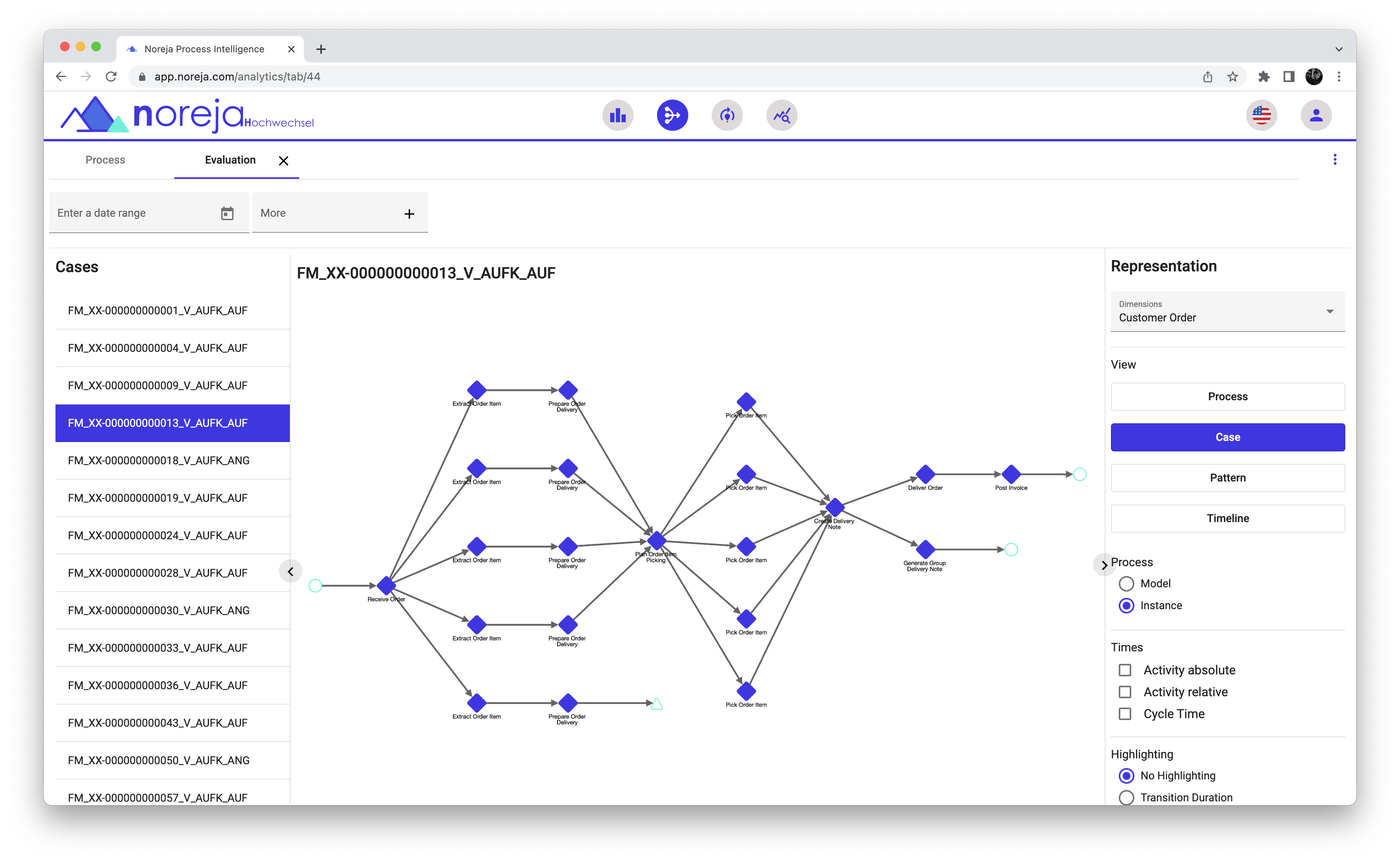
Figure 11: CEG created with the Noreja Approach.

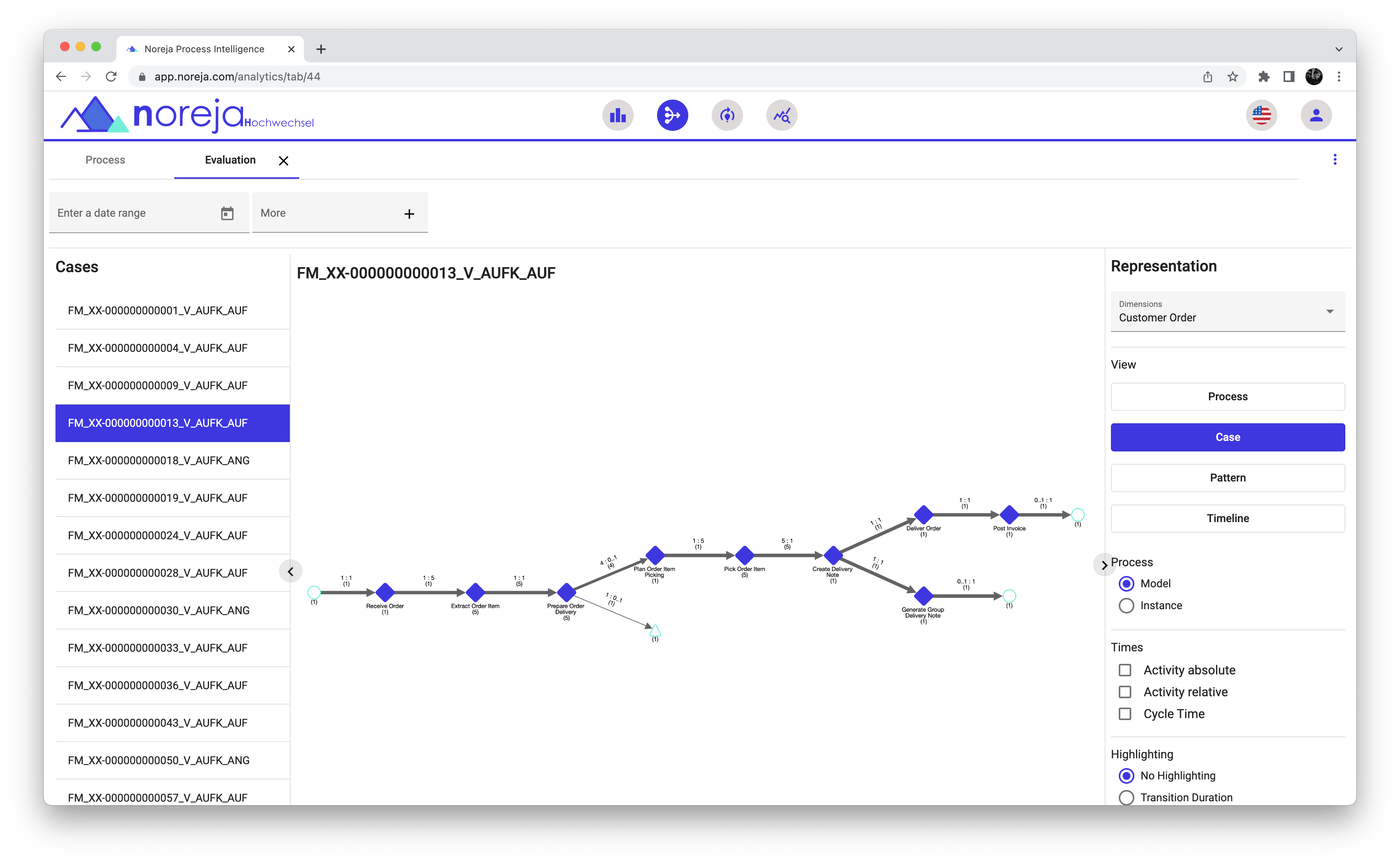
Figure 12: 1 aggregation level ACEG created with the Noreja Approach.

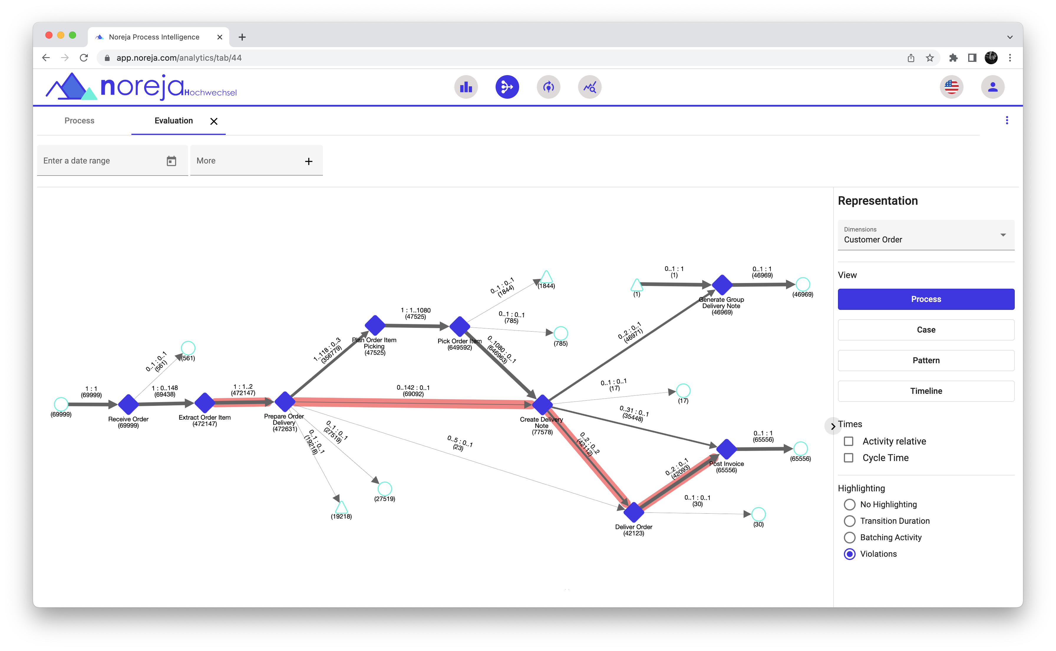
Figure 13: With violation highlighting.

4.3 Qualitative Analysis

To evaluate the presented Noreja Approach, we first compare the structure it learned, i.e., the CEG with the structure mined from state-of-the-art approaches. More specifically, we compare the 3 aggregation level ACEG produced with the Noreja Approach (cf. Figure 14) with the Business Process Model and Notation (BPMN) 2.0 model created by Split Miner 2.0 [39] (cf. Figure 15) and a DFG created by PMTK [40], which is a UI for PM4Py [41] (cf. Figure 16).

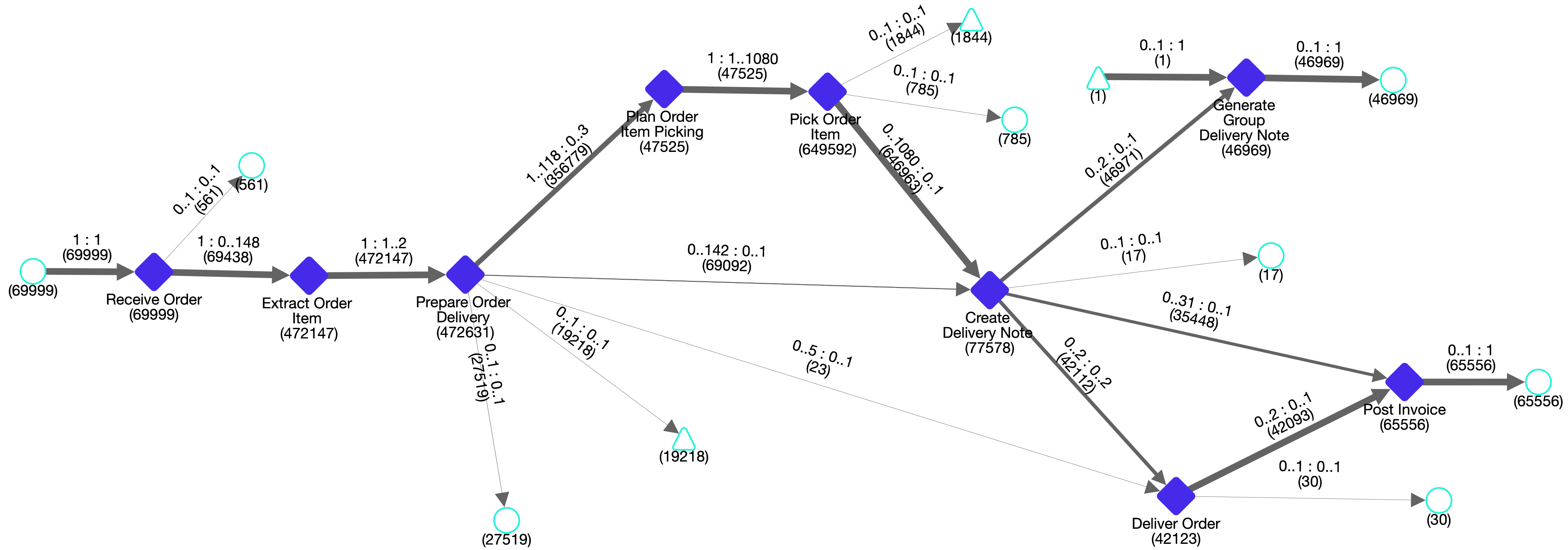
Figure 14: 3 aggregation level ACEG created with the Noreja Approach.

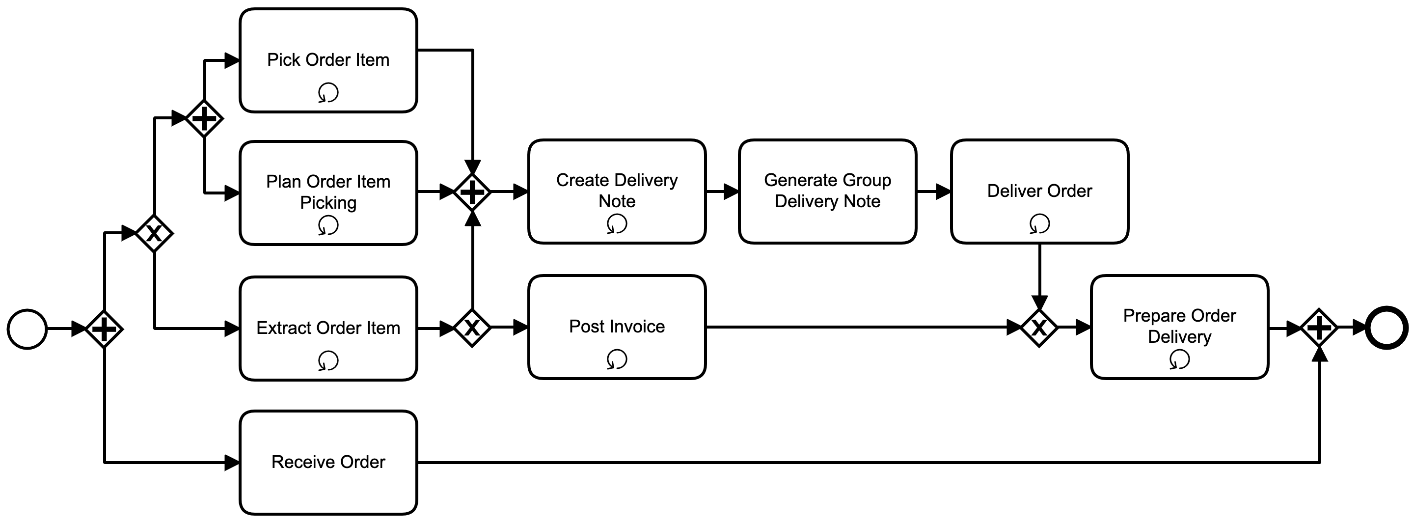
Figure 15: BPMN created by Split Miner with a concurrency threshold of 0.2. Note: The activities got re-arranged for a clearer view.

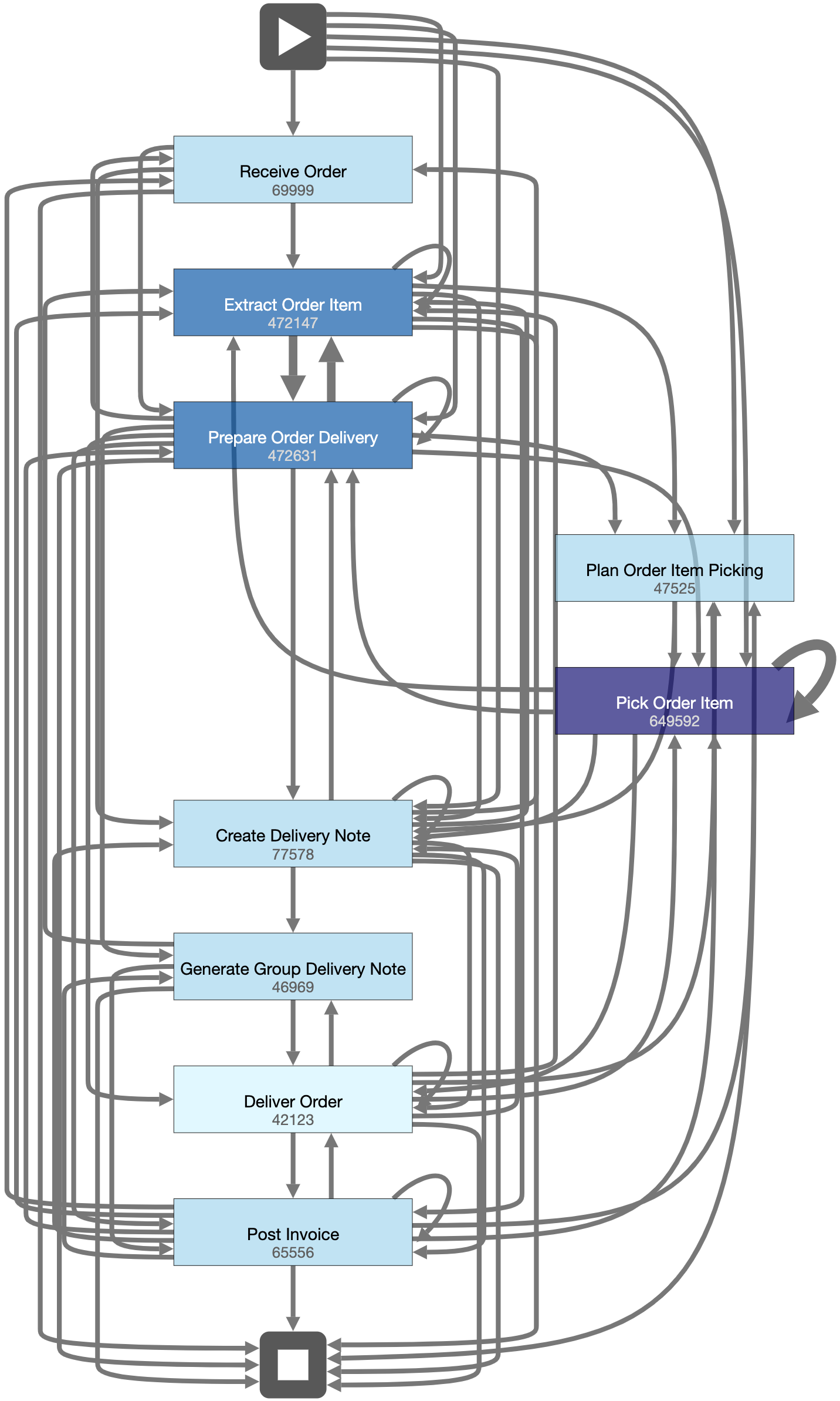
Figure 16: DFG created with PMTK.

As can be seen in Figure 16, which shows the DFG discovered by PM4Py, the DFG contains several spurious relationships that are not expected considering the causality among the relations (see Figure 10). For instance, most events contain self-loops as a byproduct of the 1:N, N:1, and N:M relationships in the database schema. They stem from separate execution sub-streams that create spurious direct-follows observations. However, this kind of self-loops are not possible in the actual database schema of the ERP system. Another example of a spurious relationship is the relationship from the Pick Order Item event to the Prepare Order Delivery event. This relationship suggests loops of the kind $\langle$ Prepare Order Delivery, Plan Order Item Picking, Pick Order Item, Prepare Order Delivery, … $\rangle$, which contradict the causal relationships of the event sequences (cf. Figure 10) and the database schema. These kind of loops are not present in the dataset, but a by-product of creating the process model without considering the causal relationships. In comparison, the ACEG created by the Noreja Approach, depicted in Figure 14, does not contain these spurious relationships, i.e., the ACEG does not contain self-loops and does not contain the relationship between Pick Order Item and Prepare Order Delivery. The reason for this is that the Noreja Approach uses the causal knowledge defined by the process analyst shown in Figure 10.

When we compare the discovered BPMN from Split Miner 2.0 (cf. Figure 15) with the expected order of activities (cf. Figure 10), we can see that some activity orders got discovered correctly. For instance, the BPMN defines that before Delivery Order there has to be a Create Deliver Node event. Another similarity is that each process instance has a Receive Order event. However, there are also differences. According to the causality among the relations (cf. Figure 10), the event Prepare Order Delivery is executed before the event Deliver Order. However, in the discovered process model the order is the other way around, which violates the causality between these events. Another difference is that according to the expected process, the events Plan Order Item Picking and Pick Order Item are executed in sequence. In the discovered process model, they are executed in parallel. This can be attributed to how the original ERP system creates the Extract Order Item and Prepare Order Delivery events. After a new order is stored, the events Extract Order Item and Prepare Order Delivery are automatically created and stored shortly after another. In some cases, the automatic creation and storage of the Prepare Order Delivery events are faster (in the millisecond range) than the creation and storage of the events Extract Order Item. Similar to the DFG created by PM4Py, most of the activities contain self-loops. These self-loops are again a by-product of the database schemas 1:N, N:1, and N:M relationships. When we compare the BPMN with the ACEG created with the Noreja Approach, we can see that by using the causal knowledge from the CPT, the order of the activities is preserved. Moreover, by using the CPT, the Noreja Approach overcomes the problem of self-loops.

4.4 Quantitative Analysis

Next, we compare the conformance of the DFG discovered by PM4Py and the ACEG created with the Noreja Approach by comparing them with the causality relations defined (cf. Figure 10). As a metric, we calculate for each causal relationship, i.e., for each pair in $\prec$, the ratio between the quantity of the expected relations to the unexpected one. For instance, when we consider the defined causality relationship Receive Order $\prec$ Extract Order Item and calculate the ratio for the ACEG shown in Figure 14 we get 69,438 / 561 (0.81%) since we have a quantity of 69,438 from Receive Order to Extract Order Item (the expected relationship) and a quantity of 561 from Receive Order to the end (the unexpected relationship). We perform this calculation for the DFG created by PM4Py and the ACEG created with the Noreja Approach. We do not consider the BPMN discovered by Split Miner since it does not show quantities. The resulting ratios for the DFG created by PM4Py can be found in Table 3 and for the ACEG in Table 4. In addition, Table 5 shows for the ACEG the ratio between the quantity of relationships without temporal violations (as defined in Section 3.3.3) to the quantities of relationships with a temporal violation.

As can be seen in the total column of Table 3 and Table 4, most unexpected relationships quantities are higher in the case of the DFG than for the ACEG. For instance, the relationship between Pick Order Item and Create Delivery Note has a ratio of 46,124 / 603,468 (1,308.36%) for the DFG and a ratio of 646,963 / 2,629 (0.41%) for the ACEG. In the case of the DFG, the huge amount of unexpected relationships stems from self-loops (due to 1:N relationships in the database schema), but also from relationships from Pick Order Item to activities at the beginning of the process e.g., Extract Order Item. In the case of the latter, these unexpected relationships stem from situations in which the order got updated e.g., a product was added at a later point in time.

By considering the causal knowledge defined in the CPT, the Noreja Approach does not suffer from the 1:N relationship problem and thus has a smaller amount of unexpected relationships. The situation of unexpected relationships when an order got updated, does not add an unexpected relationship to the ACEG, but it results in a temporal violation of a relationship before the current event, e.g., before Pick Order Item. For instance, as can be seen in Table 5 the relationship from Prepare Order Delivery to Create Delivery Note contains multiple violations, suggesting that some Prepare Order Delivery events happened after Create Delivery Note.

Another difference can be seen for the ratio of the relationship Post Invoice to the end. In case of PM4Py’s DFG, we have a ratio of 63,758 / 1,798 (2.82%) and in case of Noreja’s ACEG we have 65556 / 0 (0.00%). As can be seen in Figure 16 the event Post Invoice has outgoing relationships to all other events in the case of the DFG, despite the fact that this event should be the last one. Again the reasons for the number of unexpected relationships are updates of the orders after the Post Invoice event was already created.

To quantify the resulting conformance to the defined CPT, we use the following metric based on the unexpected relationships and temporal violations:

• For PM4Py’s DFG, we calculate the cumulative quantity of all unexpected relationships from Table 3.

• For Noreja’s ACEG, we also calculate the cumulative quantity of all unexpected relationships from Table 4. Furthermore, we add the quantity of all relationships with a temporal violation according to Table 5, when they are on an expected relationship.

By using this metric, we obtain a score of 1,153,710 for the DFG discovered by PM4Py and a score of 165,124 for the ACEG created by the Noreja Approach. While the absolute numbers are not directly expressive, the numbers relative to each other are. The significantly smaller score of the ACEG suggests a much simpler process with higher conformance to the defined causality. It has to be noted that in the case of the DFG, the main part of the high score is due to the self-loops in the case of the Pick Order Item event and the relationship between the Extract Order Item and Prepare Order Delivery events. As discussed above, the automatic creation and storage of the Prepare Order Delivery events are sometimes faster than the creation and storage of the events Extract Order Item, which leads to alternating executions. However, when the unexpected relationships that start with Extract Order Item and Prepare Order Delivery events are ignored, the cumulative score of the DFG is 687,053, which is still much higher than the one for the ACEG.

4.5 Discussion

In the following, we reflect on how of predefined requirements in Section 2.2 are covered by the Noreja Approach.

The first requirement, Input Data representing Causal Event Structure, is about the input data that is used for the PM technique. As discussed in Section 3.2.3, our approach uses as a data input source the relational database to keep and represent the causality of the events. We hereby concur with works of Lu et al. [9], Fahland [25], and Berti and van der Aalst [13] who also interpret the underlying cardinalities of relational databases as one potential source of causal knowledge. This stands in contrast to the usage of event logs that mainly discard this kind of causality knowledge due to flattening [6]. Nevertheless, we would like to note that other potential input data sources (e.g., document databases, graph databases, key-value databases, or other NoSQL databases) should not be generally excluded here.

Subsequently, the second requirement, External Knowledge about Causal Event Structure, is concerned with the integration or enrichment of real-world domain knowledge to observe the causality between the events correctly. Li et al. [24] also resort to this type of information source, particularly for reconstructing and evaluating temporal and sequential orders but they are not using a structured procedure to add this kind of information. By contrast, and in the case of the presented CPM approach, this domain knowledge is incorporated by the CPT. During the transformation of the source input data, which originates from the relational database, this CPT is used as an information source for the causality between the events. As can be seen in the evaluation, by using the CPT, the Noreja Approach is able to create simpler process models than those created by state-of-the-art approaches. Additionally, it provides the opportunity to change the provided external knowledge flexibly ex-post (e.g., in case the external environment conditions change).

While the first two requirements are concerned with transforming the input data to the graph structure, the 3 and 4 requirements are concerned with the analysis of the data itself. As defined in Section 2.2, the 3 requirement, Event Cardinalities, is about the importance of correctly calculating the cardinalities of events in order to cope with the challenge of convergence versus divergence, also called batching behavior. In fact, this challenge has been addressed by a multitude of papers [9, 11, 13]. Nevertheless, most of the approaches do not consider cardinalities under the constraint of causality. As our evaluation shows, by leveraging causal knowledge, the Noreja Approach does not suffer from the problems stemming from the 1:N, N:1, and N:M relationships in the database schema. This avoids spurious self-loops and complex structures and provides the means to accurately calculate the cardinalities of the events as well as for the relationships which is mentioned by van der Aalst [6] as one of the most fundamental flaws of common PM approaches.

The 4 requirement, Aggregation of Causal Event Structures, deals with the question of how an analyst can be supported by providing the process in different levels of detail. As discussed in Section 3.2.4 and shown in the evaluation, our approach fulfills this requirement by providing each process instance as a CEG, i.e., the most detail level, and different aggregations of them as ACEGs. Other approaches also recognize the rationale for more diverse analysis methods, e.g., by handling multi-instantiated sub-process models [22], representing it into a process cube [28], or synthesizing Petri net structures [33]. Somehow, at higher aggregated levels, this often leads to the loss of the causal relationships or the blurring of cardinalities.

5 Conclusion

Recent PM research has spent considerable effort on developing and improving automatic process discovery algorithms. The outcome of these efforts are algorithms with high precision and recall but also complex Spaghetti models. In this paper, we developed a novel approach to Causal Process Mining (CPM) that is based on knowledge about causal relations. We presented the Noreja Approach that utilizes the causal knowledge defined in a Causal Process Template (CPT) to create a Causal Event Graph (CEG). Subsequently, different aggregation levels of these CEGs are created in form of Aggregated Causal Event Graph (ACEG). The Noreja approach then exploits these structures to offer multiple operations to analyze the process on different levels of aggregation and from various perspectives.

Our evaluation demonstrates the benefits of CPM and the consideration of causal knowledge during process discovery. The evaluation shows that the presented Noreja Approach creates less complex process models than the compared approaches. One of the main reasons for this is the fact that the Noreja Approach does not struggle with the problem that is inherent with the 1:N, N:1, and N:M relations of database schema. A second reason for less complex models is attributable to how the Noreja Approach handles situations like later updates of a process instance. Instead of resulting in additional relationships, which complicate the process model, such situations result in temporal violations.

We are currently working on various extensions of the CPM and the Noreja Approach. First, we plan to analyze and develop different kinds of additional visualization, filtering, and aggregation methods. Second, we investigate support for drift detection for the process by detecting drifts in the CEGs and ACEGs using machine learning. Third, since the transformed CEGs and ACEGs are graph structures, different analysis approaches from graph theory can be used. For the area of process analysis, especially analysis techniques like Link Prediction or Graph Embeddings can be beneficial. For instance, predicting the next executed activity of an unfinished process or predicting the remaining execution duration. Alternatively, using graph embeddings e.g., Node2Vec [42] or Graph2Vec [43] provides the means to perform advanced levels of clustering.

Appendix A Evaluation Results

Table 3, 4, and 5 contain the results of the quantitative analysis (cf. Section 4.4) that compares PM4Py with the Noreja Approach.

Table 3: Ratio between the Expected Relationships Quantity and the Unexpected Relationships Quantity (Expected / Unexpected) of the Process Model Discoverd by PM4Py.

Target of Relationship Start Receive Order Extract Order Item Prepare Order Delivery Plan Order Item Picking Pick Order Item Create Delivery Note Generate Group Delivery Note Deliver Order Post Invoice End Total (%) Source of Relationship Start 0 / 0 68,836 / 1,163 0 / 0 0 / 0 0 / 0 0 / 0 0 / 0 0 / 0 0 / 0 0 / 0 0 / 0 68,836 / 1,163 (1.69%) Receive Order 0 / 0 0 / 0 68,103 / 1,896 0 / 0 0 / 0 0 / 0 0 / 0 0 / 0 0 / 0 0 / 0 0 / 0 68,103 / 1,896 (2.78%) Extract Order Item 0 / 0 0 / 0 0 / 0 433,119 / 39,023 0 / 0 0 / 0 0 / 0 0 / 0 0 / 0 0 / 0 0 / 0 433,119 / 39,023 (9.01%) Prepare Order Delivery 0 / 0 0 / 0 0 / 0 0 / 0 44,997 / 427,634 0 / 0 0 / 0 0 / 0 0 / 0 0 / 0 0 / 0 44,997 / 427,634 (950.36%) Plan Order Item Picking 0 / 0 0 / 0 0 / 0 0 / 0 0 / 0 47,524 / 1 0 / 0 0 / 0 0 / 0 0 / 0 0 / 0 47,524 / 1 (0.00%) Pick Order Item 0 / 0 0 / 0 0 / 0 0 / 0 0 / 0 0 / 0 46,124 / 603,468 0 / 0 0 / 0 0 / 0 0 / 0 46,124 / 603,468 (1308.36%) Create Delivery Note 0 / 0 0 / 0 0 / 0 0 / 0 0 / 0 0 / 0 0 / 0 46,414 / 30,626 538 / 30,626 0 / 0 0 / 0 46,952 / 30,626 (65.23%) Generate Group Delivery Note 0 / 0 0 / 0 0 / 0 0 / 0 0 / 0 0 / 0 0 / 0 0 / 0 0 / 0 0 / 0 24 / 46,945 24 / 46,945 (195,604.17%) Deliver Order 0 / 0 0 / 0 0 / 0 0 / 0 0 / 0 0 / 0 0 / 0 0 / 0 0 / 0 40,967 / 1,156 0 / 0 40,967 / 1,156 (2.28%) Post Invoice 0 / 0 0 / 0 0 / 0 0 / 0 0 / 0 0 / 0 0 / 0 0 / 0 0 / 0 0 / 0 63,758 / 1,798 63,758 / 1,798 (2.28%) End 0 / 0 0 / 0 0 / 0 0 / 0 0 / 0 0 / 0 0 / 0 0 / 0 0 / 0 0 / 0 0 / 0 0 / 0 (0.00%)

Table 4: Ratio between the Expected Relationships Quantity and theUnexpected Relationships Quantity (Expected / Unexpected) of the 3 ACEG Aggregation Level created by Noreja Approach.

Target of Relationship Start Receive Order Extract Order Item Prepare Order Delivery Plan Order Item Picking Pick Order Item Create Delivery Note Generate Group Delivery Note Deliver Order Post Invoice End Total Source of Relationship Start 0 / 0 69,999 / 1 0 / 0 0 / 0 0 / 0 0 / 0 0 / 0 0 / 0 0 / 0 0 / 0 0 / 0 69,999 / 1 (0.00%) Receive Order 0 / 0 0 / 0 69,438 / 561 0 / 0 0 / 0 0 / 0 0 / 0 0 / 0 0 / 0 0 / 0 0 / 0 69,438 / 561 (0.81%) Extract Order Item 0 / 0 0 / 0 0 / 0 472,147 / 0 0 / 0 0 / 0 0 / 0 0 / 0 0 / 0 0 / 0 0 / 0 472,147 / 0 (0.00%) Prepare Order Delivery 0 / 0 0 / 0 0 / 0 0 / 0 356,779 / 116,184 0 / 0 0 / 0 0 / 0 0 / 0 0 / 0 0 / 0 356,779 / 116,184 (32.56%) Plan Order Item Picking 0 / 0 0 / 0 0 / 0 0 / 0 0 / 0 47,525 / 0 0 / 0 0 / 0 0 / 0 0 / 0 0 / 0 47,525 / 0 (0.00%) Pick Order Item 0 / 0 0 / 0 0 / 0 0 / 0 0 / 0 0 / 0 646,963 / 2,629 0 / 0 0 / 0 0 / 0 0 / 0 646,963 / 2,629 (0.41%) Create Delivery Note 0 / 0 0 / 0 0 / 0 0 / 0 0 / 0 0 / 0 0 / 0 46,971 / 35,465 42,112 / 35,465 0 / 0 0 / 0 89,083 / 35,465 (39.81%) Generate Group Delivery Note 0 / 0 0 / 0 0 / 0 0 / 0 0 / 0 0 / 0 0 / 0 0 / 0 0 / 0 0 / 0 46,969 / 0 46,969 / 0 (0.00%) Deliver Order 0 / 0 0 / 0 0 / 0 0 / 0 0 / 0 0 / 0 0 / 0 0 / 0 0 / 0 42,093 / 30 0 / 0 42,093 / 30 (0.07%) Post Invoice 0 / 0 0 / 0 0 / 0 0 / 0 0 / 0 0 / 0 0 / 0 0 / 0 0 / 0 0 / 0 65,556 / 0 65,556 / 0 (0.00%) End 0 / 0 0 / 0 0 / 0 0 / 0 0 / 0 0 / 0 0 / 0 0 / 0 0 / 0 0 / 0 0 / 0 0 / 0 (0.00%)

Table 5: Ration between Quantity without Temporal Violation and Quantity with Temporal Violation (Quantity without Violation / Quantity with Violation) of the Aggregation Level 3 ACEG created by Noreja Approach.

Target of Relationship Start Receive Order Extract Order Item Prepare Order Delivery Plan Order Item Picking Pick Order Item Create Delivery Note Generate Group Delivery Note Deliver Order Post Invoice End Total (%) Source of Relationship Start 0 / 0 69,999 / 0 0 / 0 0 / 0 0 / 0 0 / 0 0 / 0 1 / 0 0 / 0 0 / 0 0 / 0 70,000 / 0 (0.00%) Receive Order 0 / 0 0 / 0 69,438 / 0 0 / 0 0 / 0 0 / 0 0 / 0 0 / 0 0 / 0 0 / 0 561 / 0 69,999 / 0 (0.00%) Extract Order Item 0 / 0 0 / 0 0 / 0 461,962 / 10,185 0 / 0 0 / 0 0 / 0 0 / 0 0 / 0 0 / 0 0 / 0 461,962 / 10,185 (2.20%) Prepare Order Delivery 0 / 0 0 / 0 0 / 0 0 / 0 356,779 / 0 0 / 0 68,057 / 1,035 0 / 0 23 / 0 0 / 0 47,069 / 0 471,928 / 1,035 (0.22%) Plan Order Item Picking 0 / 0 0 / 0 0 / 0 0 / 0 0 / 0 44,486 / 0 0 / 0 0 / 0 0 / 0 0 / 0 0 / 0 44,486 / 0 (0.00%) Pick Order Item 0 / 0 0 / 0 0 / 0 0 / 0 0 / 0 0 / 0 646,963 / 0 0 / 0 0 / 0 0 / 0 2,629 / 0 649,592 / 0 (0.00%) Create Delivery Note 0 / 0 0 / 0 0 / 0 0 / 0 0 / 0 0 / 0 0 / 0 46,970 / 0 42,112 / 13 35,448 / 0 17 / 0 124,548 / 13 (0.01%) Generate Group Delivery Note 0 / 0 0 / 0 0 / 0 0 / 0 0 / 0 0 / 0 0 / 0 0 / 0 0 / 0 0 / 0 46,969 / 0 46,969 / 0 (0.00%) Deliver Order 0 / 0 0 / 0 0 / 0 0 / 0 0 / 0 0 / 0 0 / 0 0 / 0 0 / 0 42,034 / 69 30 / 0 42,064 / 30 (0.07%) Post Invoice 0 / 0 0 / 0 0 / 0 0 / 0 0 / 0 0 / 0 0 / 0 0 / 0 0 / 0 0 / 0 65,556 / 0 65,556 / 0 (0.00%) End 0 / 0 0 / 0 0 / 0 0 / 0 0 / 0 0 / 0 0 / 0 0 / 0 0 / 0 0 / 0 0 / 0 0 / 0 (0.00%)

References

- van der Aalst [2016] W. M. P. van der Aalst, Process Mining - Data Science in Action, Second Edition, Springer, 2016.
- Leemans et al. [2018] S. J. Leemans, D. Fahland, W. M. P. van der Aalst, Scalable process discovery and conformance checking, Software & Systems Modeling 17 (2018) 599–631.
- Buijs et al. [2014] J. C. Buijs, B. F. van Dongen, W. M. P. van der Aals, Quality dimensions in process discovery: The importance of fitness, precision, generalization and simplicity, International Journal of Cooperative Information Systems 23 (2014) 1440001.
- Augusto et al. [2019] A. Augusto, R. Conforti, M. Dumas, M. La Rosa, A. Polyvyanyy, Split miner: automated discovery of accurate and simple business process models from event logs, Knowledge and Information Systems 59 (2019) 251–284.
- Augusto et al. [2018] A. Augusto, R. Conforti, M. Dumas, M. La Rosa, F. M. Maggi, A. Marrella, M. Mecella, A. Soo, Automated discovery of process models from event logs: Review and benchmark, IEEE Transactions on Knowledge and Data Engineering 31 (2018) 686–705.
- van der Aalst [2011] W. M. P. van der Aalst, On the representational bias in process mining, in: S. Reddy, S. Tata (Eds.), 20th IEEE International Workshops on Enabling Technologies: Infrastructures for Collaborative Enterprises, WETICE 2011, Paris, France, 27-29 June 2011, Proceedings, IEEE Computer Society, 2011, pp. 2–7. URL: https://doi.org/10.1109/WETICE.2011.64. doi:10.1109/WETICE.2011.64.
- van der Aalst et al. [2011] W. van der Aalst, A. Adriansyah, A. K. A. De Medeiros, F. Arcieri, T. Baier, T. Blickle, J. C. Bose, P. Van Den Brand, R. Brandtjen, J. Buijs, et al., Process mining manifesto, in: International Conference on Business Process Management, Springer, 2011, pp. 169–194.
- Gerke et al. [2009] K. Gerke, J. Mendling, K. Tarmyshov, Case construction for mining supply chain processes, in: International Conference on Business Information Systems, Springer, 2009, pp. 181–192.
- Lu et al. [2015] X. Lu, M. Nagelkerke, D. van de Wiel, D. Fahland, Discovering interacting artifacts from ERP systems, IEEE Trans. Serv. Comput. 8 (2015) 861–873.
- van der Aalst [2019] W. M. P. van der Aalst, Object-centric process mining: Dealing with divergence and convergence in event data, in: P. C. Ölveczky, G. Salaün (Eds.), Software Engineering and Formal Methods - 17th International Conference, SEFM 2019, Oslo, Norway, September 18-20, 2019, Proceedings, volume 11724 of Lecture Notes in Computer Science, Springer, 2019, pp. 3–25. URL: https://doi.org/10.1007/978-3-030-30446-1_1. doi:10.1007/978-3-030-30446-1\_1.
- Li et al. [2018] G. Li, E. G. L. de Murillas, R. M. de Carvalho, W. M. P. van der Aalst, Extracting object-centric event logs to support process mining on databases, in: CAiSE Forum, volume 317 of Lecture Notes in Business Information Processing, Springer, 2018, pp. 182–199.
- de Murillas et al. [2020] E. G. L. de Murillas, H. A. Reijers, W. M. P. van der Aalst, Case notion discovery and recommendation: automated event log building on databases, Knowl. Inf. Syst. 62 (2020) 2539–2575.
- Berti and van der Aalst [2020] A. Berti, W. van der Aalst, Extracting multiple viewpoint models from relational databases, in: P. Ceravolo, M. van Keulen, M. T. Gómez-López (Eds.), Data-Driven Process Discovery and Analysis, Springer International Publishing, Cham, 2020, pp. 24–51.
- Andrews et al. [2020] R. Andrews, C. van Dun, M. Wynn, W. Kratsch, M. Röglinger, A. ter Hofstede, Quality-informed semi-automated event log generation for process mining, Decision Support Systems 132 (2020) 113265. URL: https://www.sciencedirect.com/science/article/pii/S0167923620300208. doi:https://doi.org/10.1016/j.dss.2020.113265.
- Esser and Fahland [2021] S. Esser, D. Fahland, Multi-dimensional event data in graph databases, J. Data Semant. 10 (2021) 109–141. URL: https://doi.org/10.1007/s13740-021-00122-1. doi:10.1007/s13740-021-00122-1.
- Pearl [2019] J. Pearl, The seven tools of causal inference, with reflections on machine learning, Comm. of the ACM 62 (2019) 54–60.
- van der Aalst [2019] W. M. van der Aalst, A practitioner’s guide to process mining: Limitations of the directly-follows graph, Procedia Computer Science 164 (2019) 321–328.
- Jans et al. [2019] M. Jans, P. Soffer, T. Jouck, Building a valuable event log for process mining: an experimental exploration of a guided process, Enterprise Information Systems 13 (2019) 601–630.
- Ciccio et al. [2018] C. D. Ciccio, F. M. Maggi, M. Montali, J. Mendling, On the relevance of a business constraint to an event log, Inf. Syst. 78 (2018) 144–161.
- Gerke et al. [2009] K. Gerke, A. Claus, J. Mendling, Process mining of rfid-based supply chains, in: 2009 IEEE Conference on Commerce and Enterprise Computing, IEEE, 2009, pp. 285–292.
- Waibel et al. [2020] P. Waibel, C. Novak, S. Bala, K. Revoredo, J. Mendling, Analysis of business process batching using causal event models, in: S. J. J. Leemans, H. Leopold (Eds.), Process Mining Workshops - ICPM 2020 International Workshops, Padua, Italy, October 5-8, 2020, Revised Selected Papers, volume 406 of Lecture Notes in Business Information Processing, Springer, 2020, pp. 17–29. URL: https://doi.org/10.1007/978-3-030-72693-5_2. doi:10.1007/978-3-030-72693-5\_2.
- Weber et al. [2015] I. Weber, M. Farshchi, J. Mendling, J. Schneider, Mining processes with multi-instantiation, in: Proceedings of the 30th Annual ACM Symposium on Applied Computing, ACM, 2015, pp. 1231–1237.