Improved Differential Privacy for SGD via Optimal Private Linear Operators on Adaptive Streams

Abstract

Motivated by recent applications requiring differential privacy over adaptive streams, we investigate optimal instantiations of the matrix mechanism [1] in this setting. We prove fundamental theoretical results on the applicability of matrix factorizations to adaptive streams, and provide a parameter-free fixed-point algorithm for computing optimal factorizations. We instantiate this framework with respect to concrete matrices which arise naturally in machine learning, and train user-level differentially private models with the resulting optimal mechanisms, yielding significant improvements in a notable problem in federated learning with user-level differential privacy.

1 Introduction and background

An important setting for private data analysis is that of streaming inputs and outputs—often dubbed continual release. Hiding individual information is especially challenging in such settings since the arrival of one person’s data may affect all future outputs of the system. A significant line of work formalizes differential privacy (DP, [2]) under continual release and builds algorithms that meet the resulting definition (e.g. [3, 4, 5, 6, 7, 8]). One prominent application of private, continual-release algorithms is to adapt iterative optimization algorithms such as SGD so that their outputs satisfy DP [7, 6, 9].

The problem of privately computing cumulative sums plays a key role in both theory and applications. Given a set of input vectors (e.g., gradients) $\mathbf{g}_{1},\dots,\mathbf{g}_{n}$ with $\mathbf{g}_{i}\in\mathbb{R}^{d}$, the task is to approximate the sequence of prefix sums $(\mathbf{g}_{1},\mathbf{g}_{1}+\mathbf{g}_{2},\dots,\mathbf{g}_{1}+\cdots+\mathbf{g}_{n})$ while satisfying DP. Solutions to this task form the core building block in DP algorithms for online PCA [10], online marginal estimation [4, 3, 11], online top-k selection [12], and training ML models [13, 6, 14], among others. For example, a common approach to private optimization is to add noise to the gradient estimates in SGD [15, 16, 17]. Kairouz et al. [6] make the observation that the key DP primitive in such contexts is not the independent estimation of individual gradients, but rather the accurate estimation of cumulative sums of gradients. Lowering the error of the DP algorithm’s approximation to the cumulative sum translates directly to improved optimization.

The structure of continual-release algorithms imposes two major constraints: first, the algorithm must be computable online—that is, we must produce the output at a given time using only prior inputs—and second, privacy analysis must account for adaptively defined inputs—that is, the guarantee should hold even against an adversary that selects inputs based on all previous outputs of the system. In learning applications, the privacy analysis must be adaptive even when the stream or raw training examples is fixed in advance, because the points at which we compute gradients depend adaptively on the output of the mechanism so far [14].

In this paper, we revisit the design of continual-release algorithms for cumulative sums and related problems. We give new tools for analyzing privacy in the adaptive setting, new methods to design optimal (within a class) algorithms for summation-style problems, and applications to central problems in private machine learning. Although we focus on learning as the primary application of our algorithmic and analytic tools, our techniques apply to a wide range of private computations over streaming data such as online monitoring [18, 19], tracking distributional changes over data streams [20], and detection of emerging trends [21].

Prior Approaches

Prior approaches to DP approximation of cumulative sums fall broadly into two categories. First, in streaming settings, existing work is generally based on the binary-tree estimator [4, 3]. This estimator embeds the values to be summed as leaf nodes in a complete binary tree $\mathcal{T}$, with internal nodes representing the sum of all leaves below them. The mechanism views the entire tree as the object to be privately released (ensuring privacy by adding independent noise to each node). An important refinement of Honaker [22] leverages the multiple independent noisy observations of correlated values to produce lower-variance estimates of the prefix sums. Kairouz et al. [6] apply Honaker’s online variant, dubbed Honaker Online, to the follow-the-regularized-leader approach to optimization [23, 24, 25]. The tree structure of these mechanisms allows for privacy analysis in the adaptive setting, as observed by [14] and formalized by [8].

The second, more general approach to cumulative sums has previously only been applied in offline settings, in which the input is received and outputs are produced as a single batch. The idea is to view cumulative sums as a special case of linear query release (since each output is a pre-specified linear combination of the inputs). In the offline setting, the tree-based approaches can be viewed as instantiations of this widely-studied factorization framework (as in, for example, [26, 1, 27, 28, 29]). To introduce the general matrix factorization approach, consider the task of computing a private estimate of a linear mapping $\mathbf{G}\mapsto\mathbf{A}\mathbf{G}$ defined by matrix $\mathbf{A}\in\mathbb{R}^{{n\!\times\!n}}$ (assumed to be full-rank throughout this work). Given any factorization $\mathbf{A}=\mathbf{B}\mathbf{C}$, a DP estimate of $\mathbf{A}\mathbf{G}$ can be computed as

$$\widehat{\mathbf{A}\mathbf{G}}=\mathbf{B}\left(\mathbf{C}\mathbf{G}+\mathbf{Z}\right)$$ (1)

where $\mathbf{Z}$ represents a sample from a noise distribution $\mathcal{D}$. Choosing $\mathcal{D}$ in a way that appropriately depends on the sensitivity of the map $\mathbf{G}\mapsto\mathbf{C}\mathbf{G}$, one can prove privacy of the noised vector $\mathbf{C}\mathbf{G}+\mathbf{Z}$, and hence of the mapping $\mathbf{G}\mapsto\widehat{\mathbf{A}\mathbf{G}}$. For example, in the case of cumulative sums, the matrix $\mathbf{A}$ is the lower-triangular matrix $\mathbf{S}$ with 1’s on and below the diagonal; the binary tree mechanisms correspond to a matrix $\mathbf{C}_{\mathcal{T}}$ with one row per tree node (see Appendix A and Appendix C respectively). A typical choice for the noise $\mathbf{Z}$ is to select it from a spherical Gaussian distribution.

A focus of existing work (e.g. [1, 27, 28, 29]) is to choose the factorization $\mathbf{B}\mathbf{C}$ to optimize some measure of overall accuracy (such as total mean squared error) subject to a privacy constraint. However (with the exception of the independent, parallel work of Fichtenberger et al. [30]), streaming constraints and adaptive privacy were not explicitly considered. In the streaming setting, one naturally requires the $i^{th}$ element (row) of $\mathbf{A}\mathbf{G}$ to be computable using only the first $i$ elements (rows) of $\mathbf{G}$. This corresponds to requiring that the linear operator of interest $\mathbf{A}$ has a lower-triangular structure when represented as a matrix, a requirement that is met by all the matrices under consideration in this work. Distributing the $\mathbf{B}$ in Eq. 1, we see $\widehat{\mathbf{A}\mathbf{G}}=\mathbf{A}\mathbf{G}+\mathbf{B}\mathbf{Z}$. As long as $\mathbf{A}\mathbf{G}$ is lower triangular, then, any matrix mechanism can be implemented by an online algorithm, via the distribution induced by $\mathbf{B}\mathbf{Z}$. However, this observation does not address a key problem: under what conditions is the resulting mechanism adaptively private?

The applications to optimization raise their own set of critical questions: How can we efficiently compute such factorizations? Which linear operators are the appropriate ones to factorize in the case of SGD? Finally, can these factorizations actually produce improved privacy/accuracy tradeoffs for real-world machine learning tasks?

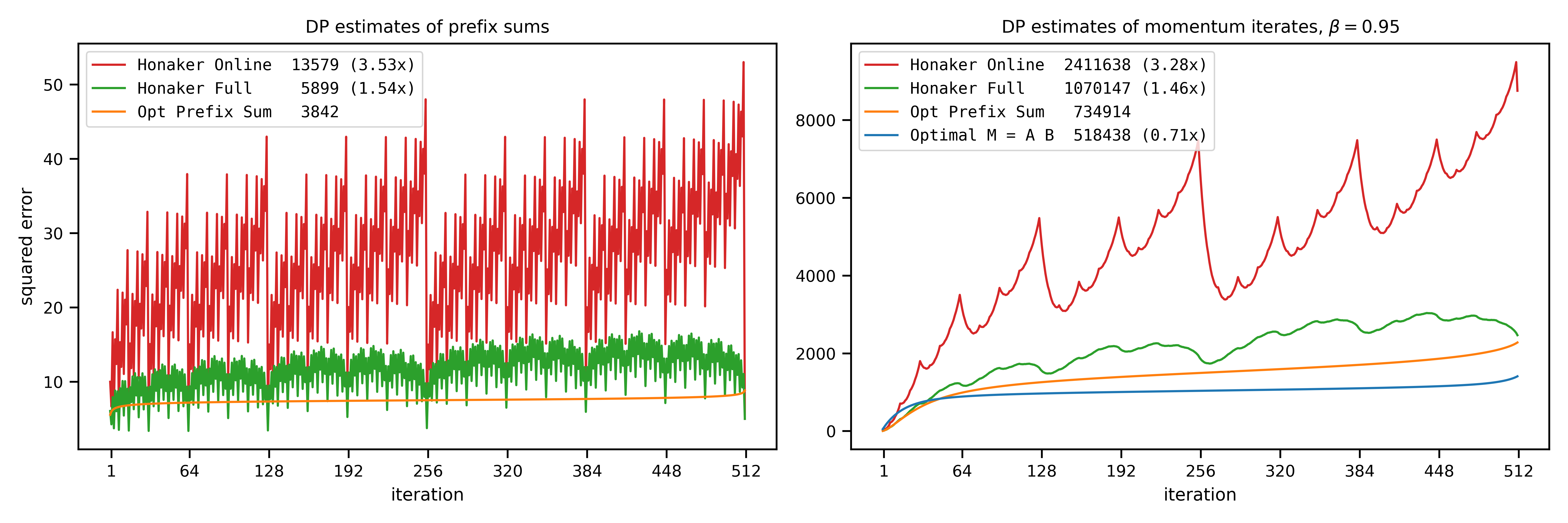
Figure 1: Left: Per-iteration squared error of three mechanisms for DP online prefix sums for $n=512$. Honaker Online and Honaker Full correspond to DP binary tree aggregation with the streaming and full Honaker estimators (respectively), while Opt Prefix Sum corresponds to the optimal matrix factorization. The tree-based mechanisms suffer from variability in the error due to the binary tree structure. Right: Squared error in the DP estimates of the iterates of momentum SGD for four mechanisms. Momentum is treated as post-processing of cumulative sums for the first 3 mechanisms, while Optimal M = B C uses the optimal factorization of the momentum matrix (see Section 4).

Contributions

We provide a deeper understanding of the matrix mechanism in the adaptive streaming setting. We show that if $\mathbf{Z}$ in Eq. 1 is drawn from a Gaussian distribution of appropriately computed variance, then the resulting mechanism is differentially private in the adaptive streaming setting, independent of the structure of $\mathbf{B}$ and $\mathbf{C}$. We make an explicit connection here with the easier-to-see privacy under adaptive streams of lower-triangular factorizations. Furthermore, we show that this property is specific to the Gaussian mechanism, and does not extend to arbitrary noise distributions.

For natural notions of error and adjacency specified in Section 3, we present a fast and parameter-free fixed-point algorithm for computing optimal factorizations and prove a local convergence guarantee for this algorithm, leveraging representations of optimal factorizations which are to our knowledge novel in the literature on the matrix mechanism. The optimal computed factorizations show a significant improvement over existing state-of-the-art private streaming prefix sum methods [22], additionally removing the artifacts of the binary tree data structure (see Fig. 1). Furthermore, our fixed-point algorithm can be two orders of magnitude more computationally efficient than existing optimization methods for the matrix mechanism [27] (though we did not explicitly compare to McKenna et al. [28]), and provides a direct bound on the duality gap which allows precise stopping criteria.

Going beyond prefix sums (which correspond to constant learning rate SGD as noted above), we construct matrix mechanisms that directly encode more sophisticated optimization algorithms as linear operators on gradients: in particular, arbitrary combinations of (data independent) learning rate schedules and momentum.

We compute optimal factorizations of these general matrices via fixed-point iterations, and use them to train user-level differentially private language models on a canonical federated learning benchmark, showing that these factorizations significantly improve the privacy/utility curve (in fact, closing 2/3rds of the gap to non-private training left by the previous state-of-the-art for single pass algorithms). For prefix sums, we show computationally-efficient structured matrices provide high-fidelity approximations to the optimal matrices, allowing implementations to scale essentially independent of the number of iterations $n$.

Notation and conventions

Matrices will be denoted by bolded capital letters (e.g. $\mathbf{A}$, $\mathbf{B}$), with some symbols reserved for special matrices, notably $\mathbf{S}$ (prefix sums) and $\mathbf{M}$ (momentum, defined in Section 4 and illustrated in Appendix A). Vectors will be denoted by bolded lowercase letters (e.g. $\mathbf{x}$, $\mathbf{y}$). For a real symmetric matrix $\mathbf{A}$, the smallest and the largest eigenvalues are denoted by $\lambda_{\min}(\mathbf{A})$ and $\lambda_{\max}(\mathbf{A})$. For a matrix $\mathbf{A}$, $\mathbf{A}^{*}$ denotes the conjugate transpose and $\mathbf{A}^{\dagger}$ denotes the Moore-Penrose pseudoinverse; a star as in $\mathbf{X}^{\star}$ indicates a matrix that is optimal in a way made clear by context. $\operatorname{diagpart}$ represents the operation of taking the diagonal elements of a matrix; $\operatorname{diag}$ represents embedding a vector argument on the diagonal of a matrix. Additional notation is summarized in Appendix A.

2 Privacy for adaptive streams

In this section, we provide structural results that clarify the classes of mechanisms/algorithms for cumulative sums and other linear computations in the continual release model [4, 3] that remain private even when the inputs stream is defined adaptively. In the continual release model, a mechanism receives a stream of inputs $\mathbf{G}=[\mathbf{g}_{1},\ldots,\mathbf{g}_{n}]$ and produces a stream of outputs $\mathbf{a}_{1},...,\mathbf{a}_{n}$, where output $\mathbf{a}_{i}$ is intended to approximate some function of the prefix $\mathbf{g}_{1},...,\mathbf{g}_{i}$ and must be generated before $\mathbf{g}_{i+1}$ is received. We specify which parts of the input can depend on a single person’s data via a neighbor relation $\mathcal{N}$ on data streams. Two streams are neighbors if they differ in one person’s data. For example, if one person’s data directly affects exactly one input in the stream (“event-level privacy”), then we say two data streams are neighboring if they differ in exactly one element (that is, they are at Hamming distance 1).

The original works on continual release analyzed privacy in a nonadaptive model: a mechanism $\mathcal{M}$ is $(\varepsilon,\delta)$-differentially private [31, 32] for nonadaptive continual release if, for all pairs of adjacent data streams $\mathbf{G},\mathbf{H}$, the corresponding distributions on output streams $\mathcal{M}(\mathbf{G})$ and $\mathcal{M}(\mathbf{H})$ are $(\varepsilon,\delta)$-indistinguishable, denoted $\mathcal{M}(\mathbf{G})\approx_{\varepsilon,\delta}\mathcal{M}(\mathbf{H})$. That is, for all events $E$, we have $\Pr[\mathcal{M}(\mathbf{G})\in E]\leq e^{\varepsilon}\Pr(\mathcal{M}(\mathbf{H})\in E)+\delta$ and $\Pr(\mathcal{M}(\mathbf{H})\in E)\leq e^{\varepsilon}\Pr(\mathcal{M}(\mathbf{G})\in E)+\delta$. (A variant of this definition tailored to differentially private gradient descent, with a precise instantiation of the neighborhood notion is presented in Definition J.1 in the appendix.)

In many use cases—including those arising in iterative gradient-based optimization algorithms—the nonadaptive model is inadequate, since the inputs $\mathbf{g}_{i}$ may be generated in real time as a function of previous outputs $\mathbf{a}_{1},...,\mathbf{a}_{i-1}$. To summarize the more general, adaptive definition [14, 8], consider an adversary that adaptively defines two input sequences $\mathbf{G}=(\mathbf{g}_{1},\dots,\mathbf{g}_{n})$ and $\mathbf{H}=(\mathbf{h}_{1},\dots,\mathbf{h}_{n})$. The adversary must satisfy the promise that these sequences correspond to neighboring data sets. The privacy game proceeds in rounds. At round $t$, the adversary generates $\mathbf{g}_{t}$ and $\mathbf{h}_{t}$. The game accepts these if the input streams defined so far are valid, meaning that there exist completions $(\tilde{\mathbf{g}}_{t+1},...,\tilde{\mathbf{g}}_{n})$ and $(\tilde{\mathbf{h}}_{t+1},...,\tilde{\mathbf{h}}_{n})$ so that $((\mathbf{g}_{1},...,\mathbf{g}_{t},\tilde{\mathbf{g}}_{t+1},...,\tilde{\mathbf{g}}_{n}),(\mathbf{h}_{1},...,\mathbf{h}_{t},\tilde{\mathbf{h}}_{t+1},...,\tilde{\mathbf{h}}_{n}))\in\mathcal{N}\,.$ For example, in the case of event-level privacy, the game simply checks that the two streams differ in at most one position so far.

The game is parameterized by a bit $\text{\sf side}\in{\{0,1\}}$ which is unknown to the adversary but constant throughout the game. The game hands either $\mathbf{g}_{t}$ or $\mathbf{h}_{t}$ to the mechanism $\mathcal{M}$, depending on side. The mechanism’s output $\mathbf{a}_{t}$ is then sent to the adversary. The privacy requirement is that the adversary’s views with $\text{\sf side}=0$ and $\text{\sf side}=1$ be $(\varepsilon,\delta)$ indistinguishable. One can substitute other relevant notions of indistinguishability like those from CDP [33, 34], Renyi DP [35], or Gaussian DP [36]. The mechanisms we consider generally satisfy Gaussian DP.

The nonadaptive version of the definition is weaker but easier to work with. It is therefore natural to look for classes of mechanisms for which the two definitions are equivalent (and thus for which a nonadaptive privacy proof implies the more general guarantee). We first observe that such a transfer statement holds for “pure” $\varepsilon$-DP (in which $\delta=0$). We defer all the proofs to Appendix D.

Proposition 2.1.

Every mechanism that is $(\varepsilon,0)$ nonadaptively DP in the continual release model satisfies the adaptive version of the definition, with the same parameters.

Unfortunately, not all privacy proofs for the nonadaptive model transfer to the adaptive setting. Indeed, we show that there are additive-noise mechanisms (which simply add noise from a pre-defined distribution to some function of the data) that are nonadaptively $(\varepsilon,\delta)$-DP, but not private in the adaptive setting (Appendix D.1).

Adaptive privacy for Gaussian noise addition mechanisms

In Theorem 2.1 we show that every matrix mechanism with Gaussian noise addition that is $(\varepsilon,\delta)$-DP in the nonadaptive model is also private in the adaptive setting:

Theorem 2.1.

Let $\mathbf{A}\in\mathbb{R}^{n\times n}$ be a lower-triangular full-rank query matrix, and let $\mathbf{A}=\mathbf{B}\mathbf{C}$ be any factorization with the following property: for any two neighboring streams of vectors $\mathbf{G}\,,\mathbf{H}\in\mathbb{R}^{n\times d}$, we have $\|\mathbf{C}(\mathbf{G}-\mathbf{H})\|_{F}\leq\kappa$. Let $\mathbf{Z}\sim\mathcal{N}(0,\kappa^{2}\sigma^{2})^{n\times d}$ with $\sigma$ large enough so that $\mathcal{M}(\mathbf{G})=\mathbf{A}\mathbf{G}+\mathbf{B}\mathbf{Z}=\mathbf{B}(\mathbf{C}\mathbf{G}+\mathbf{Z})$ satisfies $(\varepsilon,\delta)$-DP (or $\rho$-zCDP or $\mu$-Gaussian DP) in the nonadaptive continual release model. Then, $\mathcal{M}$ satisfies the same DP guarantee (with the same parameters) even when the rows of the input are chosen adaptively.

To prove this we crucially use the rotational invariance of spherical Gaussian distribution, yielding distributional equivalence of an orbit of mechanisms: those factorizations expressible as $\mathbf{B}\mathbf{U}\mathbf{U}^{*}\mathbf{C}$ for $\mathbf{U}$ unitary. This observation can similarly be leveraged to show a subtly distinct fact:

Proposition 2.2.

For any factorization $\mathbf{A}=\mathbf{B}\mathbf{C}$ where $\mathbf{A}$ is lower-triangular, there exists a factorization $\mathbf{A}=\widehat{\mathbf{B}}\widehat{\mathbf{C}}$ which induces a distributionally equivalent matrix mechanism under Gaussian noise with $\widehat{\mathbf{B}}$ and $\widehat{\mathbf{C}}$ lower triangular. This factorization can be explicitly computed from $\mathbf{A}=\mathbf{B}\mathbf{C}$ via an appropriate LQ decomposition. Normalizing to all-nonnegative entries on the diagonal, this factorization is unique.

3 Computing optimal factorizations

Once one writes down the matrix mechanism as in Eq. 1, it is natural to seek factorizations that minimize the error $\widehat{\mathbf{A}\mathbf{G}}-\mathbf{A}\mathbf{G}$ in some metric of choice. In this section we consider the expected squared reconstruction error of the estimate $\widehat{\mathbf{A}\mathbf{G}}$, which has previously been noted as an appropriate formulation of error for the setting of training private ML models [6, Theorem 5]. Further, for simplicity we restrict our attention to the single-pass setting. That is, for the remainder of the paper we will assume:

Definition 3.1.

Two data matrices $\mathbf{G}$ and $\mathbf{H}$ in $\mathbb{R}^{n\times d}$ will be considered to be neighboring if they differ by a single row, with the $\ell_{2}$-norm of the difference in this row at most $\zeta$.

Under this notion of sensitivity, one can make the estimation of any query $\mathbf{A}\mathbf{G}$ $(\varepsilon,\delta)$-DP via Theorem 3.1, which via Theorem 2.1 immediately extends to adaptive streams. It is worth mentioning that while we state the analytic vairance for the Normal distribution to satisfy $(\varepsilon,\delta)$-DP, in practice we arrive at the required (and tighter) variance via empirical privacy accounting methods like zero concentrated DP (zCDP) accounting [33], or privacy loss distribution (PLD) accounting [37].

Theorem 3.1 (Adapted from [1]).

Consider a query matrix $\mathbf{A}\in\mathbb{R}^{n\times n}$ along with a fixed factorization $\mathbf{A}=\mathbf{B}_{n\times n}\mathbf{C}_{n\times n}$ with $\gamma=\max_{i\in[n]}\left\|\mathbf{C}_{[:,i]}\right\|_{2}$, the maximum column norm of $\mathbf{C}$. Let $\mathbf{G}\in\mathbb{R}^{{n\times d}}$ be a fixed (non-adaptive) data matrix with each row of $\mathbf{G}$ having $\ell_{2}$-norm at most $\zeta$. The algorithm that outputs $\mathbf{B}\left(\mathbf{C}\mathbf{G}+\mathbf{Z}\right)$ with $\mathbf{Z}\sim\mathcal{N}\left(0,\frac{\gamma^{2}\zeta^{2}\left(2\log(1/\delta)+\varepsilon\right)}{\varepsilon^{2}}\right)^{n\times d}$ satisfies $(\varepsilon,\delta)$-DP.

In this setting, with $\mathbf{Z}\sim\mathcal{N}\left(0,\gamma^{2}\right)^{n\times d}$ following Theorem 3.1 (which ensures a fixed level of privacy when $\zeta=1$ for an arbitrary factorization factorization $\mathbf{A}=\mathbf{B}\mathbf{C}$) the expected reconstruction error can be computed directly as $\mathcal{L}(\mathbf{B},\mathbf{C})$ [1, Proposition 9], [27, Equation 3],

$$\gamma^{2}(\mathbf{C})=\max_{i\in[1,\dots,n]}\left\|\mathbf{C}_{[:,i]}\right\|_{2}^{2}\qquad\text{and}\qquad\mathcal{L}(\mathbf{B},\mathbf{C})=\gamma^{2}(\mathbf{C})\left\|\mathbf{B}\right\|_{F}^{2}.$$ (2)

As has been noted [1, 27], Eq. 2 can be manipulated to yield a convex program, for which hand-tuned algorithms exist [27, Section 4]. Theorem 2.1 shows, for the first time, that arbitrary factorizations found by minimizing this optimization problem can be applied in the adaptive streaming setting.

We present an alternative characterization of these optima, which reformulates the optimization problem as a fixed-point problem. We show that simply iterating an explicit mapping converges to this fixed point from an appropriate initialization, and observe numerically that the associated algorithm achieves fast, global convergence.

Since the Moore-Penrose pseudoinverse yields the minimal $\ell_{2}$-norm solution to a set of underdetermined linear equations [38, Theorem 2.1.1], we note that for a fixed $\mathbf{C}$ term (of any dimensionality), the optimal $\mathbf{B}$ may be expressed as $\mathbf{B}_{\mathbf{C}}^{\star}=\mathbf{A}\mathbf{C}^{\dagger}$. Since $\mathbf{A}=\mathbf{B}\mathbf{C}$ implies $\mathbf{A}=\big{(}\alpha\mathbf{B}\big{)}\big{(}\frac{1}{\alpha}\mathbf{C}\big{)}$, for any linear space of matrices $\mathbf{V}$, we may express the optimization problem of interest as

$$\min_{\mathbf{C}\in\mathbf{V}}\mathcal{L}\left(\mathbf{A}\mathbf{C}^{\dagger},\mathbf{C}\right)=\min_{\mathbf{C}\in\mathbf{V}}\gamma^{2}(\mathbf{C})\left\|\mathbf{A}\mathbf{C}^{\dagger}\right\|_{F}^{2}=\min_{\mathbf{C}\in\mathbf{V},\gamma^{2}(\mathbf{C})=1}\left\|\mathbf{A}\mathbf{C}^{\dagger}\right\|_{F}^{2}.$$ (3)

The properties of the problem Eq. 3 have been studied previously. In particular, [27, Section 3] studied a symmetric version, transforming the problem as:

$$\mathbf{X}^{\star}=\operatorname*{arg\,min}_{\mathbf{X}\text{ is PD},\mathbf{X}_{[i,i]}\leq 1,1\leq i\leq n}\mathrm{tr}(\mathbf{A}^{*}\mathbf{A}\mathbf{X}^{-1})$$ (4)

which essentially reparameterizes Eq. 3 (with $\mathbf{V}=\mathbb{R}^{n}$) in terms of $\mathbf{C}^{*}\mathbf{C}$. To recover a matrix-mechanism factorization of $\mathbf{A}$, then, one may utilize any $\mathbf{C}$ such that $\mathbf{X}^{\star}=\mathbf{C}^{*}\mathbf{C}$, e.g. $\mathbf{C}=\sqrt{\mathbf{X}^{\star}}$. Proposition 2.2 can be used to construct a lower-triangular factorization if desired.

Yuan et al. [27] show: 1) Any solution $\mathbf{X}^{\star}$ of Eq. 4 must have diagonal entries exactly 1. 2) Any solution $\mathbf{X}^{\star}$ may be taken to be strictly within the positive-definite cone, with minimal eigenvalue bounded from below in terms of the eigenvalues of $\mathbf{A}$. 3) For any full-rank $\mathbf{A}$, $\mathbf{X}\mapsto\mathrm{tr}(\mathbf{A}^{*}\mathbf{A}\mathbf{X}^{-1})$ is strictly convex over symmetric, positive-definite matrices. Therefore the solution to Eq. 4 is unique.

By analyzing Eq. 4 directly, we derive a characterization of solutions in terms of an explicit fixed-point problem, with a corresponding bound on the optimality gap.

Theorem 3.2.

The minimizer $\mathbf{X}^{\star}$ of Eq. 4 is in one-to-one correspondence with the unique fixed point of the function $\phi:\mathbb{R}^{n}_{+}\to\mathbb{R}^{n}_{+}$ defined by

$$\phi(\mathbf{v})=\operatorname{diagpart}\left(\sqrt{\operatorname{diag}(\mathbf{v})^{1/2}\,\mathbf{A}^{*}\mathbf{A}\,\operatorname{diag}(\mathbf{v})^{1/2}}\right).$$ (5)

Letting

$$\mathcal{X}(\mathbf{v})=\operatorname{diag}(\mathbf{v})^{-1/2}\left(\operatorname{diag}(\mathbf{v})^{1/2}\,\mathbf{A}^{*}\mathbf{A}\,\operatorname{diag}(\mathbf{v})^{1/2}\right)^{1/2}\operatorname{diag}(\mathbf{v})^{-1/2},$$ (6)

for the fixed point $\mathbf{v}^{\star}$ of Eq. 5, that is $\phi(\mathbf{v}^{\star})=\mathbf{v}^{\star}$, we have $\mathbf{X}^{\star}=\mathcal{X}(\mathbf{v}^{\star})$, and this pair $\left(\mathbf{X}^{\star},\mathbf{v}^{\star}\right)$ satisfies

$$\mathbf{A}^{*}\mathbf{A}=\mathbf{X}^{\star}\operatorname{diag}\left(\mathbf{v}^{\star}\right)\mathbf{X}^{\star}.$$ (7)

Further, for any $\mathbf{v}\in\mathbb{R}^{n}_{+}$, the objective value of the primal problem Eq. 4 is lower-bounded by

$$\mathrm{tr}\big{(}\operatorname{diag}(\mathbf{v})(2\mathcal{X}(\mathbf{v})-\mathbf{I})\big{)},$$ (8)

and this bound is tight for $\mathbf{v}=\mathbf{v}^{\star}$.

The sum of the elements of $\phi$ represents a quantity of independent interest in quantum information, the so-called Jozsa fidelity [39, 40], while $\mathcal{X}$ represents the matrix geometric mean of $\mathbf{A}^{*}\mathbf{A}$ and $\operatorname{diag}(\mathbf{v})^{-1}$ [41, 42]. These connections give some hope that the fixed point of $\phi$ can be understood in a direct manner. We can show local, though not yet global, convergence of the iterates of $\phi$ to this fixed point.

Theorem 3.3.

$\phi$ defined in Eq. 5 is a local contraction around its fixed point in a suitable metric, and hence there is a neighborhood of this fixed point in which iterates of $\phi$ converge to this fixed point. The precise norm of this contraction, and the size of the neighborhood in which convergence is guaranteed, can both be estimated in terms of minimum and maximum eigenvalues of $\mathbf{A}$.

This result can be shown by linearizing the mapping $\phi$ around its fixed point and performing an involved estimate of its Jacobian at the fixed point. As such, it is implied by Theorem E.1, which states that the linearization of $\phi$ around its fixed point is a contraction in a suitable metric, and therefore the Banach fixed-point theorem applies.

Remark. Notably missing from quantification of the contraction is the dimension $n$. Indeed, the argument is dimension-independent in a strong sense: it applies to the suitably generalized definition of $\phi$ where $\mathbf{A}$ is any bounded linear operator on a Hilbert space with bounded inverse.

Empirical performance of the fixed-point method

Experimentally, iterating the mapping $\phi$ is sufficient to converge to the global optimum extremely quickly from any initial point (modulo potential numerical issues in computing the matrix square root, discussed in Section E.4). Yuan et al. [27, Algorithm 1] design an algorithm with globally linear and locally quadratic convergence rate, with similar asymptotics to iterating $\phi$ (each dominated by an $n^{3}$ term), though at the cost of introducing a parameter $T$. Iterating $\phi$, on the other hand, is parameter-free. We implemented [27, Algorithm 1] as well as a direct gradient-descent-based method to numerically compare convergence speed. As a canonical benchmark, we computed optimal factorizations of the $512\times 512$ and $2048\times 2048$ prefix-sum matrices $\mathbf{S}$ (Appendix G provides a visualization of this optimal factorization). Our fixed-point algorithm was significantly faster than either of the alternatives to compute optima, computing a lower-loss matrix for the larger problem in less than 3 minutes than either alternative found in over 80 minutes. See Section E.4 for details. Further, via Eq. 8, our approach provides an optimality certificate that allows a precise specification of the stopping criteria in terms of any target optimality gap. The speed and simplicity of our fixed-point algorithm was a significant enabler of the mechanism exploration presented in the next section.

4 The matrix mechanism for SGD

To define our gradient descent algorithm, let $\mathbf{G}\in\mathbb{R}^{n\times d}$ be the matrix of gradients, with row vector $\mathbf{g}_{i}\in\mathbb{R}^{1\times d}$ the gradient observed on iteration $i$ after clipping to norm at most $\zeta$; we abuse notation slightly by writing $\mathbf{G}_{[1:i,:]}\in\mathbb{R}^{n\times d}$, formed by taking the first $i$ rows of $\mathbf{G}$, with zeros for the as-of-yet unobserved gradient rows for iterations $i+1,\dots,n$ (the lower triangular structure of the matrices we consider will imply $\mathbf{G}_{[1:i,:]}$ vs $\mathbf{G}$ does not in fact change the value computed). With this notation, we define Algorithm 1, a general template for private SGD algorithms.

Algorithm 1 DP Matrix Factorization SGD

1:Inputs:

2:    factorization $\mathbf{M}=\mathbf{B}\mathbf{C}$

3:    overall learning rate $\eta$

4:    noise level $\sigma$, clipping norm $\zeta$

5:    examples $\chi_{i}$, $i\in\{1,\dots,n\}$

6:$\boldsymbol{\theta}_{[0,:]}:=0\in\mathbb{R}^{d}$

7:Sample $\mathbf{Z}\in\mathbb{R}^{n\times d}$, $\mathbf{Z}_{[i,j]}\!\sim\!\mathcal{N}(0,\sigma^{2})$ iid

8:for $i$ in $1,\dots,n$ do

9:     $\hat{\mathbf{g}}:=\nabla_{\boldsymbol{\theta}_{[i-1,:]}}\ell(\boldsymbol{\theta};\chi_{i})$

10:     $\mathbf{G}_{[i,:]}:=\hat{\mathbf{g}}\cdot\min\left\{\frac{\zeta}{\|\hat{\mathbf{g}}\|_{2}},1\right\}$

11:     $\boldsymbol{\theta}_{[i,:]}:=-\eta\big{(}\mathbf{M}_{[i,:]}\mathbf{G}_{[1:i,:]}+\mathbf{B}_{[i,:]}\mathbf{Z}\big{)}$

Algorithm 2 Heavy-ball momentum

1:$\boldsymbol{\theta}_{0}:=0$, $\mathbf{m}_{0}:=0$

2:for $i$ in $1,\dots,n$ do

3:     $\mathbf{m}_{i}:=\beta\cdot\mathbf{m}_{i-1}+\mathbf{g}_{i}$

4:     $\boldsymbol{\theta}_{i}:=\boldsymbol{\theta}_{i-1}-\eta_{i}\mathbf{m}_{i}$

The power of this general formulation comes largely from the following privacy guarantee:

Theorem 4.1.

Under the “replace with zero” notion of differential privacy (in Defininition J.1 in the appendix) over examples (records) $\chi_{i}$, taking $\hat{\mathbf{g}}=0$ when $\chi_{i}=\bot$, Algorithm 1 (that releases the iterates $\boldsymbol{\theta}_{[i,:]}$) satisfies equivalent $(\varepsilon,\delta)$-DP to the Gaussian mechanism with noise variance $\sigma^{2}$ applied to records with $\ell_{2}$ sensitivity at most $\zeta\gamma$, where $\gamma=\max_{i}\left\|\mathbf{C}_{[:,i]}\right\|_{2}$ is the maximum column norm of $\mathbf{C}$, and $\zeta$ is the clipping norm.

Theorem 4.1 shows that the contribution of $\mathbf{C}$ to the loss Eq. 19 is reflected in the privacy guarantee of Algorithm 1, by determining the sensitivity of the matrix mechanism Eq. 1. The contribution of $\mathbf{B}$ determines the expected squared reconstruction error of the matrix mechanism, by definition. This quantification can in turn be converted by existing analytical methods to a regret bound for convex losses:

Proposition 4.1 (Adaptation of Theorem C.1, Kairouz et al. [6]).

In the setup of Algorithm 1, let $\mathbf{M}$ be the prefix-sum matrix $\mathbf{S}$, and assume $\ell$ is convex with $\ell_{2}$-Lipschitz constant $L$. Let $\theta_{t}=\boldsymbol{\theta}_{[t,:]}$. For any $\theta^{\star}\in\mathbb{R}^{d}$,

$$\frac{1}{n}\sum_{t=1}^{n}\mathbb{E}\left[\ell(\theta_{t};\chi_{t})-\ell(\theta^{\star};\chi_{t})\right]\leq\eta L^{2}+\frac{1}{2\eta n}\left(\|\theta^{\star}\|_{2}^{2}-\|\theta_{1}\|_{2}^{2}\right)+\frac{L\sigma\eta}{\sqrt{n}}\|\mathbf{B}\|_{F}$$

We now consider different instantiations of Algorithm 1. Let $\mathbf{S}$ be the prefix-sum matrix as defined in Appendix A, and let $\mathbf{C}_{\mathcal{T}}$ be the matrix representation of the binary tree (Appendix C), so for appropriate choices of the reconstruction matrices $\mathbf{B}_{\text{hs}}$ and $\mathbf{B}_{\text{hf}}$, $\mathbf{S}=\mathbf{B}_{\text{hs}}\mathbf{C}_{\mathcal{T}}$ gives the Honaker Online mehcanism, and $\mathbf{S}=\mathbf{B}_{\text{hf}}\mathbf{C}_{\mathcal{T}}$ gives the Honaker Full mechanism. In particular, using the Honaker Online factorization in Algorithm 1 recovers the non-momentum DP-FTRL algorithm of Kairouz et al. [6].

However, Kairouz et al. [6] observed that for non-convex objectives, DP-FTRL with momentum provided superior privacy/accuracy tradeoffs. Given prefix sums, momentum can be implemented as post processing by estimating individual gradients/updates as the difference of successive cumulative sums (multiplication by $\mathbf{S}^{-1}$), and then passing these into a standard momentum SGD optimizer. We show that performance can be improved by directly incorporating momentum and a-priori learning rate schedules directly into the DP mechanism.

A basic but important observation is that momentum SGD can be expressed as a linear map of gradients $\mathbf{G}\to\mathbf{M}\mathbf{G}$. We consider the classic momentum algorithm of Polyak [43], with per-iteration learning rates $\eta_{1},\dots,\eta_{n}$ and momentum $\beta\in[0,1)$, as in Algorithm 2. Alternatively, we can express momentum SGD as a linear operator on the gradients:

Proposition 4.2.

For any $\beta\in[0,1)$, $n\geq 1$, per iteration learning rates $\eta_{1},\dots,\eta_{n}$, define the lower-triangular matrix $\mathbf{M}\in\mathbb{R}^{n\times n}$ as the product of lower-triangular matrices $\mathbf{M}^{(\eta)}$ and $\mathbf{M}^{(\beta)}$:

$$\mathbf{M}^{(\eta)}_{[i,j]}=\begin{cases}\eta_{j}&\text{$i\geq j$}\\ 0&\text{otherwise}\end{cases},\quad\mathbf{M}^{(\beta)}_{[i,j]}=\begin{cases}\beta^{i-j}&\text{$i\geq j$}\\ 0&\text{otherwise}\end{cases},\qquad\text{and}\qquad\mathbf{M}=\mathbf{M}^{(\eta)}\mathbf{M}^{(\beta)}.$$ (9)

Then, for any matrix of of per-iteration gradients $\mathbf{G}\in\mathbb{R}^{n\times d}$ with rows $[\mathbf{g}_{1},\dots,\mathbf{g}_{n}]$, the sequence of iterates $\boldsymbol{\theta}\in\mathbb{R}^{n\times d}$ with rows $[\boldsymbol{\theta}_{1},\dots\boldsymbol{\theta}_{n}]$ produced by Algorithm 2 can equivalently be written $\boldsymbol{\theta}=-\mathbf{M}\mathbf{G}$.

We apply the fixed-point algorithm of Section 3 to $\mathbf{M}$ to obtain optimal matrix mechanisms $\mathbf{M}=\mathbf{B}\mathbf{C}$, which indeed leads to improved performance. We can also convert mechanisms that produce DP prefix sums to produce momentum iterates via post processing: given any matrix mechanism for the prefix sum problem given as a factorization $\mathbf{S}=\mathbf{B}\mathbf{C}$, we can convert this to a mechanism for momentum as $\mathbf{M}=\hat{\mathbf{B}}\mathbf{C}$ where $\hat{\mathbf{B}}=\mathbf{M}\mathbf{S}^{-1}\mathbf{B}$. Straightforward calculations show this representation is equivalent to the “Momentum Variant” of DP-FTRL [6]. This allows us to consistently evaluate the mechanisms in terms of the total variance (squared error) induced in the outputs by unit-variance noise $\mathbf{Z}$ in the mechanism via Eq. 2. Table 1 summarizes the four instantiations of Algorithm 1 for any choise of $\mathbf{M}$; note in particular that for $\beta=0$ and a fixed learning rate schedule $\eta_{i}=1$, $\mathbf{M}=\mathbf{S}$. Fig. 1 compares the per-step squared error of the DP momentum iterates for these methods for $\beta=0$ (prefix sums, as a constant $\eta=1$ is used) and $\beta=0.95$.

Mechanism	$\mathbf{B}$	$\mathbf{C}$	s.t. $\mathbf{M}=\mathbf{B}\mathbf{C}$
Honaker Online	$\mathbf{M}\mathbf{S}^{-1}\mathbf{B}_{\text{hs}}$	$\mathbf{C}_{\mathcal{T}}$	Equivalent to DP-FTRL of Kairouz et al. [6]
Honaker Full	$\mathbf{M}\mathbf{S}^{-1}\mathbf{B}_{\text{hf}}$	$\mathbf{C}_{\mathcal{T}}$
Opt Prefix Sum	$\mathbf{M}\mathbf{S}^{-1}\mathbf{B}_{S}^{*}$	$\mathbf{C}_{S}^{\star}$	for optimal $\mathbf{S}=\mathbf{B}_{S}^{\star}\mathbf{C}_{S}^{\star}$
Optimal M = B C	$\mathbf{B}_{M}^{\star}$	$\mathbf{C}^{\star}_{M}$	for optimal $\mathbf{M}=\mathbf{B}_{M}^{\star}\mathbf{C}_{M}^{\star}$

Table 1: Instantiations of Algorithm 1 for various factorizations of the SGD matrix $\mathbf{M}=\mathbf{B}\mathbf{C}$.

Computational efficiency

Some care is necessary for the efficient implementation of Algorithm 1, particularly the computation of $\mathbf{M}_{[i,:]}\mathbf{G}_{[1:i,j]}+\mathbf{B}_{[i,:]}\mathbf{Z}$ on line 11. First, we observe that via Proposition 4.2 we can efficiently compute the $\mathbf{M}\mathbf{G}$ term via Algorithm 2, rather than as a matrix operation. This leaves the computation of the noise $\mathbf{B}_{[i,:]}\mathbf{Z}.$ For applications to ML, $d$ could be $10^{6}-10^{9}$, and with even $n=10^{4}$ rounds (iterations) this might make the total calculation quite expensive if not prohibitive. With an efficient TensorFlow implementation, in our experiments with $d\approx 4\times 10^{6}$ and $n=2048$, we found we could compute the noise directly. However, for larger applications we show (in Appendix H) that one can compute structured matrices that well-approximate the optimal $\mathbf{B}^{\star}$ for the prefix sum matrix while allowing for $\mathcal{O}(d)$ calculation of the per-round noise vectors (on par with that of the binary tree mechanism, which can also provide computational efficiency with a careful implementation, see Table 2). The key is to observe the diagonal dominance of the optimal $\mathbf{B}^{\star}$ (see Appendix G), leading to an approximation $\hat{\mathbf{B}}$ that is the sum of a lower-triangular $d$-banded matrix with the remaining entries in the lower triangle extracted from a low-rank approximation computed via alternating-least-squares.

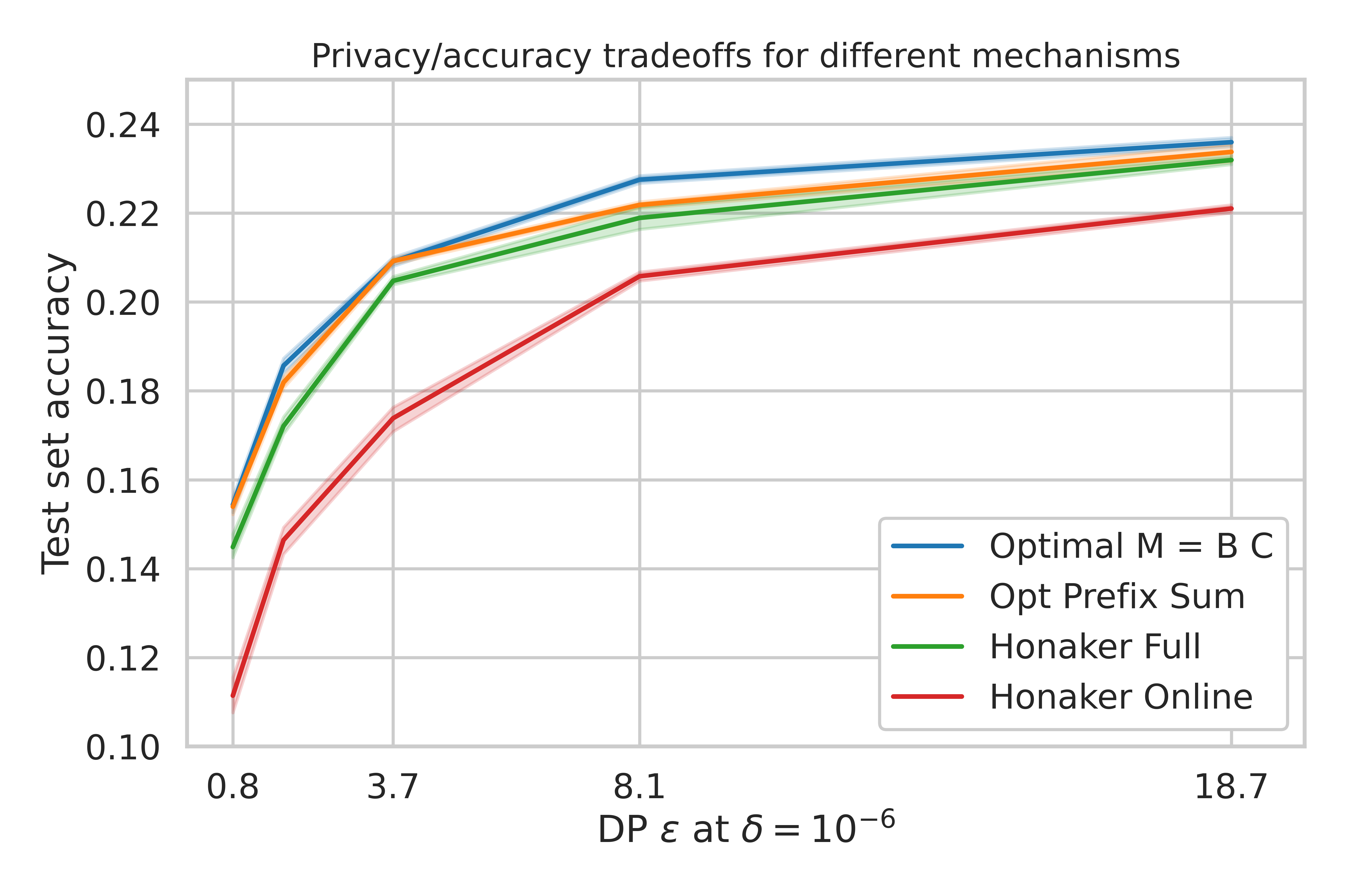
Figure 2: Test accuracy for the StackOverflow next-word-prediction task. A grid search over client and server learning rates and momentum $\beta$, with the best hyperparameters selected based on validation set accuracy. We then re-ran 11 repetitions with the best hyperparameters and report the mean test set accuracy with confidence intervals. All models trained with 100 clients per round and a constant learning rate schedule.

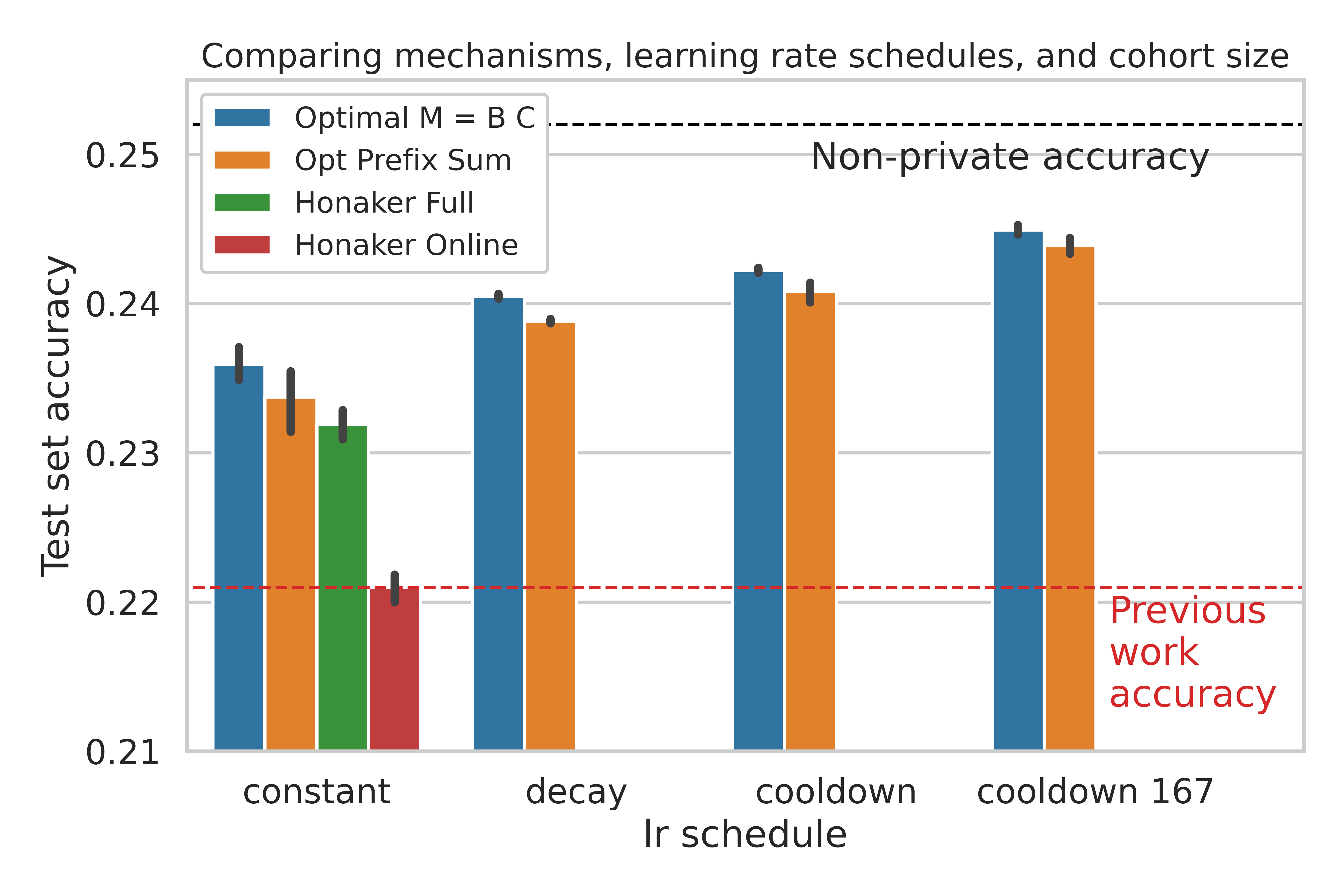
Figure 3: Test accuracy for mechanisms incorporating learning rate decay in the manner of Section 4 at $\varepsilon=18.9$. The red horizontal line represents test accuracy of previous state of the art at $\varepsilon=18.9$; highest horizontal line, test accuracy of non-private model. The final bar group shows learning rate cooldown with $167$ clients/round, the maximum possible for a single training pass of 2048 training rounds.

5 Experimental results

The results of Sections 2 and 4 significantly expand the space of mechanisms which can be used in training ML models with differential privacy in the single-pass setting. In this section we demonstrate that these techniques can in fact significantly advance the state-of-the-art in private ML.

User-level privacy for language models

Private training is particularly important for generative language models: training language models on data from the right distribution is critical for utility (e.g., user input in a mobile keyboard [44, 45]), but this data is often privacy-sensitive. Further, language models have been shown to be capable of memorizing training data [46, 47, 48]. In this setting it is important to consider user-level DP, where the neighbor relation of the DP guarantee covers all of the training examples (tokens) from any one user, as opposed to a single training example [49]. In our setting, this corresponds to ensuring that each user’s examples contribute to a bounded $\ell_{2}$-norm update to a single row of $\mathbf{X}$ (Definition 3.1). This is accomplished by extending Algorithm 1 in the natural way to Federated Averaging [50]: instead of a single gradient, we take $\mathbf{g}_{i}$ to be the sum of the individually-clipped-to-$\zeta$ updates of all users (100 or 167 in our experiments) participating in the current round, with each user contributing to a single round over the course of training.

For these reasons, we focused on the StackOverflow next-word prediction problem, introduced in [51] and publicly hosted in TensorFlow-Federated (TFF) [52]. This task was explored extensively in [6], and serves as a major benchmark in federated learning, used in [51, 6, 53, 54, 55], and others. The StackOverflow dataset contains sufficiently many clients to support single-pass algorithms with 100 clients per round, similar to the baseline setup of [6]. For this reason, we are able to provide true $(\varepsilon,\delta)$ privacy quantifications for the models we train.

Results

We compare the four mechanisms of Table 1 on this problem; full experimental methodology, as well as additional plots (e.g., for validation error vs. training rounds) are provided in Appendix I. Fig. 3 shows that even with constant learning rates, our matrix factorization approaches significantly outperform the previous state-of-the-art across a range of privacy $\varepsilon$’s. Further, thanks to the results of Section 2, we are able to apply the Honaker Full mechanism for comparison. Fig. 3 shows that applying learning rate decay (dropping the learning rate by $0.15\times$ for the last 512 rounds) and learning rate cooldown (linearly dropping the learning rate from $1.0\times$ to $0.05\times$ over the last 512 rounds) show added improvements. These experiments all used 100 clients/round as in [6], but the rightmost bars shows increasing this to 167 (the maximum possible for a single pass of 2048 rounds) provides additional accuracy. In combination, these techniques close more than 2/3rds of the gap between private and non-private training.

6 Conclusions

We have shown the general applicability of the Gaussian matrix mechanism to the adaptive streaming setting, introduced a highly efficient mechanism of determining optimal (in the sense of total $\ell_{2}^{2}$ error) matrix mechanisms, used this approach to directly incorporate momentum and learning rate schedules into the DP mechanism, and empirically demonstrated the resulting private SGD (or FedAvg in the federated setting) substantially improves on the state of the art for private ML.

While our focus has been on the application of these techniques to gradient-based optimization algorithms, we emphasize that the problem of producing private estimates for linear queries in the adaptive streaming setting is a fundamental DP primitive of much broader applicability, as noted in the introduction, and so our work immediately leads to improvements in those applications as well.

Finally, our work raises numerous natural follow-up questions which we hope will inspire subsequent work; we sketch these in Appendix B.

Appendix A Summary of notation and important matrices

The prefix-sum linear operator $\mathbf{S}$, and its inverse:

$$\mathbf{S}:=\begin{pmatrix}1&0&0&\cdots&0\\ 1&1&0&\cdots&0\\ 1&1&1&\cdots&0\\ \vdots&\vdots&\vdots&\ddots&\vdots\\ 1&1&1&\cdots&1\end{pmatrix}\qquad\text{and}\qquad\mathbf{S}^{-1}:=\begin{pmatrix}1&0&0&\cdots&0\\ -1&1&0&\cdots&0\\ 0&-1&1&\cdots&0\\ \vdots&\vdots&\vdots&\ddots&\vdots\\ 0&0&0&\cdots&1\end{pmatrix}.$$ (10)

Representation of momentum SGD as a linear operator $\mathbf{M}=\mathbf{M}^{(\eta)}\mathbf{M}^{(\beta)}$:

$$\mathbf{M}^{(\eta)}:=\begin{pmatrix}\eta_{1}&0&0&\cdots&0\\ \eta_{1}&\eta_{2}&0&\cdots&0\\ \eta_{1}&\eta_{2}&\eta_{3}&\cdots&0\\ \vdots&\vdots&\vdots&\ddots&\vdots\\ \eta_{1}&\eta_{2}&\eta_{3}&\cdots&\eta_{n}\end{pmatrix}\qquad\text{and}\qquad\mathbf{M}^{(\beta)}:=\begin{pmatrix}1&0&0&\cdots&0\\ \beta&1&0&\cdots&0\\ \beta^{2}&\beta&1&\cdots&0\\ \vdots&\vdots&\vdots&\ddots&\vdots\\ \beta^{n-1}&\beta^{n-2}&\beta^{n-3}\cdots&1\end{pmatrix}$$ (11)

Summary of notation

The following table briefly summarizes notation used throughout this work.

$\mathbf{g}_{i}\in\mathbb{R}^{d}$	Input (e.g. gradient) on step $i$ of the online process.
$\mathbf{G}\in\mathbb{R}^{n\times d}$	Matrix of all inputs, $\mathbf{g}_{i}=\mathbf{G}_{[i,:]}$.
$\mathbf{A}\in\mathbb{R}^{n\times n}$	Lower-triangular linear query matrix to be factorized as $\mathbf{A}=\mathbf{B}\mathbf{C}$.
$\lambda_{\min}(\mathbf{A})$, $\lambda_{\max}(\mathbf{A})$.	Smallest and largest eigenvalues of real matrix $\mathbf{A}$.
$\mathbf{A}^{*}$	Conjugate transpose of $\mathbf{A}$.
$\mathbf{X}^{\star}$	A matrix $\mathbf{X}$ that is “optimal” in a context-dependent sense.
$\mathbf{A}^{\dagger}$	Moore-Penrose pseudoinverse of matrix $\mathbf{A}$.
$\mathbf{A}_{[i,j]}$	The $(i,j)^{\text{th}}$ entry of matrix $\mathbf{A}$.
$\mathbf{A}_{[i,:]}$ and $\mathbf{A}_{[:,j]}$	The $i^{\text{th}}$ row and $j^{\text{th}}$ column.

Appendix B Future work.

Each of the sections above poses a unique set of problems for future investigation, many interrelated. We will highlight only some of the major questions left open by this work.

Scalable mechanism implementations

Theorem 2.1 shows that we need not restrict ourselves to any particular matrix structure in order to guarantee privacy over adaptive streams. Appendix H shows we can find efficient approximations for the case of prefix sums, but this leaves open the question of whether better or more general approximations are possible, or whether one can optimize over structures that allow efficient implementations directly.

Analysis and numerics of $\phi$

Theorem 3.3 represents a usable convergence result for iterates of the mapping $\phi$; on the other hand, it represents only partial progress on the conjecture of global convergence of these iterates. Though we factorized many distinct matrices in the course of writing this paper, we generated no reason to doubt this conjecture. Indeed, the speed of convergence of these iterates of $\phi$ (see Section E.4) only makes this method more intriguing from a theoretical perspective. Further, though the fixed-point method utilized to compute these factorizations has enabled significant exploration (as detailed in Section 4), it still does not quite represent the optimal algorithm for computing these optima: an explicit formula for the fixed point of $\phi$ would clearly be desirable, and might yield interesting insights into the structure of these optimal matrices.

We finally note that for production use, additional care will be needed to ensure that claimed privacy guarantees fully account for floating point imprecision.

Adaptive choice of the query

While the sequence of gradients during optimization is adaptive (subsequent gradients depend on previous gradients), as we have seen SGD with momentum can be expressed as a fixed linear operator $\mathbf{M}$. Data-independent learning rate schedules can be incorporated into an optimization matrix in a similar fashion, again allowing for optimal DP matrix mechanisms. However, adaptive learning rate schedules such as AdaGrad amount to a non-linear (and adaptive, not fixed) map on the gradient sequence; hence a very interesting open question is to see if the approach used here can be extended to adaptive optimization algorithms.

Appendix C Tree aggregation and decoding as matrix factorization

As mention in Section 1, the tree data structure $\mathcal{T}$ is linear in the data matrix $\mathbf{G}$ (all of its internal nodes are linear combinations of the rows $\mathbf{G}$). Therefore the mapping $\mathbf{G}\to\mathcal{T}$ can be represented as multiplication by a matrix. We present a simple recursive construction of this matrix. The base case is the $1\times 1$ matrix $[1]$, which we will denote by $\mathbf{C}_{\mathcal{T}}^{(1)}$; we will define $\mathbf{C}_{\mathcal{T}}^{(k)}\in\mathbb{R}^{(2^{k}-1)\times(2^{k-1})}$ to be the matrix constructed by duplicating $\mathbf{C}_{\mathcal{T}}^{(k-1)}$ on the diagonal, and adding one more row of constant $1$s. That is,

$$\mathbf{C}_{\mathcal{T}}^{(1)}:=\begin{pmatrix}1\end{pmatrix},\mathbf{C}_{\mathcal{T}}^{(2)}:=\begin{pmatrix}1&0\\ 0&1\\ 1&1\end{pmatrix},\mathbf{C}_{\mathcal{T}}^{(3)}:=\begin{pmatrix}1&0&0&0\\ 0&1&0&0\\ 1&1&0&0\\ 0&0&1&0\\ 0&0&0&1\\ 0&0&1&1\\ 1&1&1&1\end{pmatrix},$$ (12)

and so on. Each row of $\mathbf{C}_{\mathcal{T}}^{(k)}\mathbf{G}$ can be seen readily to correspond to a node of the binary tree $\mathcal{T}$ constructed from $\mathbf{G}$, assuming $n=2^{k-1}$ (possibly padding with zeros if needed).

With this construction, it is straightforward to represent both vanilla differentially-private binary tree aggregation and the Honaker variant as instantiations of the matrix factorization framework. For a vector $\mathbf{x}$ with $n=2^{k-1}$ entries, vanilla binary-tree aggregation can be represented as $\mathbf{C}=\mathbf{C}_{\mathcal{T}}^{(k)}$, $\mathbf{B}$ an appropriate $\{0,1\}$-valued matrix satisfying $\mathbf{B}\mathbf{C}=\mathbf{S}$ for prefix-sum $\mathbf{S}$. The Honaker estimators can both be computed as (real-valued) matrices also satisfying $\mathbf{B}\mathbf{C}=\mathbf{S}$, and are in fact optimal:

Proposition C.1.

For the prefix-sum matrix $\mathbf{S}$ with $n=2^{k-1}$ rows, the (non-streaming) Honaker fully efficient estimator represents the minimal-loss factorization for prefix sum $\mathbf{S}=\mathbf{B}\mathbf{C}$ for $\mathbf{C}=\mathbf{C}_{\mathcal{T}}^{(k)}$. This estimator is precisely $\mathbf{S}\mathbf{C}^{\dagger}$. The streaming Honaker estimator-from-below represents the minimal loss factorization satisfying the property that the $j^{th}$ row of $\mathbf{B}$ zeros out rows in the matrix $\mathbf{C}\mathbf{G}$ which place nonzero weight on the $i^{th}$ row of $\mathbf{G}$ for $i>j$. The Honaker estimator-from-below can be expressed similarly row-by-row with a constrained pseudoinverse of $\mathbf{C}$.

Proof.

We begin by recalling a geometric property of the Moore-Penrose pseudoinverse. Theorem 2.1.1 of [38] states that for any matrix $\mathbf{C}\in\mathbb{C}^{m\times n}$, vector $\mathbf{s}\in\mathbb{C}^{m}$, the vector $\mathbf{C}^{\dagger}\mathbf{s}$ is the minimal least-squares solution to the linear system $\mathbf{C}\mathbf{x}=\mathbf{s}$. Notice that this statement is implicitly a statement of uniqueness; $\mathbf{C}^{\dagger}\mathbf{s}$ is the unique minimal-norm solution to $\mathbf{C}\mathbf{x}=\mathbf{s}$, assuming feasability of this equation. Since the square of the Frobenius norm of the matrix $\mathbf{B}$ is the sum of the squared norms of its rows, we may apply this Theorem row-by-row to $\mathbf{B}$ to demonstrate that the minimal Frobenius norm solution $\mathbf{B}$ to $\mathbf{S}=\mathbf{B}\mathbf{C}$ for fixed $\mathbf{C}$ is $\mathbf{S}\mathbf{C}^{\dagger}$.

This minimal Frobenius norm property may be translated to a statistical perspective. That is, for a fixed matrix $\mathbf{C}$ and data matrix $\mathbf{G}$, $\mathbf{S}\mathbf{C}^{\dagger}$ represents the minimal-variance unbiased linear estimator for $\mathbf{S}\mathbf{G}$ given the noisy estimates $\mathbf{C}\mathbf{G}+\mathbf{Z}$. This is precisely the definition of Honaker’s fully efficient estimator in Section 3.4 of [22], and we have the first statement of this proposition.

The second follows similarly, but leveraging instead the geometric properties of the constrained pseudoinverse. These properties are collected in Theorem 3.6.3 of [38], and allow us to compute directly the optimal $\mathbf{B}$ under constraints that certain entries in each row must be $0$, corresponding to the constraints stated in the proposition. By construction of the matrices $\mathbf{C}_{\mathcal{T}}^{(k)}$, the property described in the statement of Proposition C.1 corresponds to restricting the linear estimator computed from a binary tree to depend only on the information below the nodes corresponding to the $1$s in a binary expansion of the index of the partial sum under consideration. This is precisely the definition of the estimator from below in Section 3.2 of [22]. ∎

Appendix D Proofs and missing details for Section 2

Proof of Proposition 2.1.

The key idea is that the nonadaptive version of the definition implies a bound on the log-odds ratio that always holds (even after the fact).

For simplicity, we focus on the case where the universe of possible outputs $\mathbf{a}$ is discrete (to avoid measurability issues).

Fix an adversary $\mathcal{A}$ and mechanism $\mathcal{M}$. Recall side is fixed an unknown to the adversary. When $\text{\sf side}=0$, the probability of a particular view $(\mathbf{G},\mathbf{H},\mathbf{a})$ is the following. We write $(\mathbf{G},\mathbf{H},\mathbf{a})\leftarrow\langle\mathcal{M},\mathcal{A}\rangle_{0}$ for the event with sequence of mechanism outputs $\mathbf{a}$, when the mechanism and the adversary are operating with the variable $\text{\sf side}=0$, and the neighboring data streams are $\mathbf{G}$ and $\mathbf{H}$ (and analogously for $\text{\sf side}=1$).

$$\Pr((\mathbf{G},\mathbf{H},\mathbf{a})\leftarrow\langle\mathcal{M},\mathcal{A}\rangle_{0})=$$

$$\Pr{\left({\mathcal{A}()=(\mathbf{g}_{1},\mathbf{h}_{1})}\right)} \times \Pr{\left({\mathcal{M}(\mathbf{g}_{1})=\mathbf{a}_{1}}\right)}\times$$

$$\Pr{\left({\mathcal{A}(\mathbf{a}_{1})=(\mathbf{g}_{2},\mathbf{h}_{2})\big{|}\mathbf{g}_{1},\mathbf{h}_{1}}\right)} \times \Pr{\left({\mathcal{M}(\mathbf{g}_{2})=\mathbf{a}_{2}\big{|}\mathbf{g}_{1},\mathbf{a}_{1}}\right)}\times$$

$$\cdots$$

$$\underbrace{\Pr{\left({\mathcal{A}(\mathbf{a}_{n-1})=(\mathbf{g}_{n},\mathbf{h}_{n})\big{|}\mathbf{g}_{1},...,\mathbf{g}_{n-1},\mathbf{h}_{1},...,\mathbf{h}_{n-1}}\right)}}_{\text{these do not depend on $\text{\sf side}$}} \times \underbrace{\Pr{\left({\mathcal{M}(\mathbf{g}_{n})=\mathbf{a}_{n}\big{|}\mathbf{g}_{1},...,\mathbf{g}_{n-1},\mathbf{a}_{1},...,\mathbf{a}_{n-1}}\right)}}_{\text{these terms depend on $\text{\sf side}$}}\,.$$

The probability of $(\mathbf{G},\mathbf{H},\mathbf{a})$ when $\text{\sf side}=1$ is similar, except that the inputs to $\mathcal{M}$ are now $\mathbf{h}_{t}$’s instead of $\mathbf{g}_{t}$’s. Either way, we get a product of $2n$ terms, half of which are about the probability of $\mathcal{A}$’s outputs, and half of which are about $\mathcal{M}$’s outputs. They key fact here is that the terms describing $\mathcal{A}$’s output are the same in both expressions. When we take the ratio, therefore, those terms cancel out and we obtain:

$$\frac{\Pr((\mathbf{G},\mathbf{H},\mathbf{a})\leftarrow\langle\mathcal{M},\mathcal{A}\rangle_{0})}{\Pr((\mathbf{G},\mathbf{H},\mathbf{a})\leftarrow\langle\mathcal{M},\mathcal{A}\rangle_{1})}\\ =\frac{\Pr{\left({\mathcal{M}(\mathbf{g}_{1})=\mathbf{a}_{1}}\right)}\times\Pr{\left({\mathcal{M}(\mathbf{g}_{2})=\mathbf{a}_{2}\big{|}\mathbf{g}_{1},\mathbf{a}_{1}}\right)}\times\cdots\times\Pr{\left({\mathcal{M}(\mathbf{g}_{n})=\mathbf{a}_{n}\big{|}\mathbf{g}_{1},...,\mathbf{g}_{n-1},\mathbf{a}_{1},...,\mathbf{a}_{n-1}}\right)}}{\Pr{\left({\mathcal{M}(\mathbf{h}_{1})=\mathbf{a}_{1}}\right)}\times\Pr{\left({\mathcal{M}(\mathbf{h}_{2})=\mathbf{a}_{2}\big{|}\mathbf{h}_{1},\mathbf{a}_{1}}\right)}\times\cdots\times\Pr{\left({\mathcal{M}(\mathbf{h}_{n})=\mathbf{a}_{n}\big{|}\mathbf{h}_{1},...,\mathbf{h}_{n-1},\mathbf{a}_{1},...,\mathbf{a}_{n-1}}\right)}}\\ =\frac{\Pr(\mathcal{M}(\mathbf{g}_{1},...,\mathbf{g}_{n})=(\mathbf{a}_{1},...,\mathbf{a}_{n}))}{\Pr(\mathcal{M}(\mathbf{h}_{1},...,\mathbf{h}_{n})=(\mathbf{a}_{1},...,\mathbf{a}_{n}))}\,.$$

This last expression involves no adversary—it is simply the ratio of the probabilities that the mechanism would have produced a given output sequence if the sequences $\mathbf{G}$ and $\mathbf{H}$ had been specified nonadaptively. Since $\mathbf{G},\mathbf{H}$ are always valid neighboring sequences, and since the nonadaptive mechanism’s guarantee holds for all output sequences, the ratio above is bounded between $e^{-\varepsilon}$ and $e^{\varepsilon}$, as desired.

∎

Proof of Theorem 2.1.

The idea is to show that, when $\mathbf{A}$ is lower triangular, the mechanism $\mathcal{M}$ can be rewritten in such a way that the adaptive privacy of $\mathcal{M}$ can be deduced from the privacy guarantees of the usual Gaussian mechanism with adaptively selected queries.

Let $(\mathbf{L},\mathbf{Q})$ form a lower-triangular LQ-factorization of $\mathbf{B}$, meaning that $\mathbf{L}$ is lower triangular, $\mathbf{Q}$ is orthonormal, and $\mathbf{B}=\mathbf{L}\mathbf{Q}$. By assumption, $\mathbf{A}$ is square and invertible, so $\mathbf{L}$ and $\mathbf{Q}$ are also square and invertible. Now consider the modified mechanism

$$\tilde{\mathcal{M}}(\mathbf{G})=\mathbf{L}(\mathbf{Q}\mathbf{C}\mathbf{G}+\mathbf{Z})\quad\text{where}\ \mathbf{Z}\sim\mathcal{N}(0,\kappa^{2}\sigma^{2})^{n\times d}$$

where $\kappa\sigma$ is the same noise standard deviation as in the original mechanism. Since $\mathbf{L}$ and $\mathbf{A}$ are lower triangular, it also means that $\mathbf{L}^{-1}\mathbf{A}=\mathbf{Q}\mathbf{C}$ is also lower triangular. This means that $\mathbf{Q}\mathbf{C}\mathbf{G}+\mathbf{Z}$ can operate in the continuous release model, as row $i$ of $\mathbf{Q}\mathbf{C}\mathbf{G}$ depends only on the first $i$ rows of $\mathbf{G}$.

Next, we further show the mechanism $\mathbf{Q}\mathbf{C}\mathbf{G}+\mathbf{Z}$ (that is, $\tilde{\mathcal{M}}$ without the post-processing operation of multiplying with $\mathbf{L}$) is an instance of the standard Gaussian mechanism for computing an adaptively defined function in the continuous release model with a guaranteed bound on the global $\ell_{2}$ sensitivity. Let $\mathbf{G},\mathbf{H}\in\mathcal{N}$ be any two fixed neighboring data streams with $\|\mathbf{C}(\mathbf{G}-\mathbf{H})\|_{F}\leq\kappa$. Then because $\mathbf{Q}$ is orthonormal we have $\|\mathbf{Q}\mathbf{C}(\mathbf{G}-\mathbf{H})\|_{F}\leq\kappa$. Letting $\mathbf{g}=\text{flatten}(\mathbf{Q}\mathbf{C}\mathbf{G})\in\mathbb{R}^{nd}$ and $\mathbf{h}=\text{flatten}(\mathbf{Q}\mathbf{C}\mathbf{H})\in\mathbb{R}^{nd}$, we have $\left\|{\mathbf{g}-\mathbf{h}}\right\|_{2}\leq\kappa$. Hence, $\mathbf{Q}\mathbf{C}\mathbf{G}+\mathbf{Z}$ is equivalent to an application of the standard Guassian mechanism on inputs $\mathbf{Q}\mathbf{C}\mathbf{G}$, and the result for adaptive streams follows from Claim D.1 below. This claim holds as the privacy loss random variable is stochastically dominated by an appropriate normally-distributed random variable (e.g., [56]).

Claim D.1 (Folklore).

Consider a streaming data vector $\mathbf{g}=[g_{1},\ldots,g_{n}]\in\mathbb{R}^{n}$ s.t. for any neighboring stream $\mathbf{h}$ we have the $\ell_{2}$-sensitivity $\left\|\mathbf{g}-\mathbf{h}\right\|_{2}\leq\kappa$. If $\mathbf{g}+\mathcal{N}(0,\kappa^{2}\sigma^{2})^{n}$ satisfy $(\varepsilon,\delta)$-DP (or $\rho$-zCDP or $\mu$-Gaussian DP) in the nonadaptive continual release model, then the same mechanism satisfies the same privacy guarantee in the adaptive continuous release model.

As $\mathbf{L}$ is lower-triangular, the adaptive streaming DP guarantee of $\mathbf{Q}\mathbf{C}\mathbf{G}+\mathbf{Z}$ extends to the mechanism $\tilde{\mathcal{M}}$ by the post-processing property of DP.

Finally, we have

$$\mathcal{M}(\mathbf{G})=\mathbf{B}(\mathbf{C}\mathbf{G}+\mathbf{Z})=\mathbf{L}(\mathbf{Q}\mathbf{C}\mathbf{G}+\mathbf{Q}\mathbf{Z}),$$

and so the only difference from $\tilde{\mathcal{M}}$ is the use of noise $\mathbf{Q}\mathbf{Z}$ vs $\mathbf{Z}$. Since $\mathbf{Q}$ is orthonormal and the Gaussian distribution is rotationally invariant, $\mathbf{Q}\mathbf{Z}$ and $\mathbf{Z}$ are identically distributed, and hence $\mathcal{M}$ and $\tilde{\mathcal{M}}$ produce identical output distributions on any fixed data set $\mathbf{G}$. Thus an adversary can simulate $\mathcal{M}$ given access to $\tilde{\mathcal{M}}$. This in turn means that the privacy guarantee of the mechanism $\tilde{\mathcal{M}}$ transfers to the mechanism $\mathcal{M}$. This completes the proof. ∎

Proof of Proposition 2.2.

The existence of such a lower-triangular factorization with identical induced matrix mechanism distribution follows directly from the proof of Theorem 2.1. The body of the proof leverages the distributional equivalence of all mechanisms expressible as

$$\left(\mathbf{B}\mathbf{U}\right)\left(\mathbf{U}^{*}\mathbf{C}\right).$$

Since $\mathbf{A}$ is lower-triangular, letting $\mathbf{U}=\mathbf{R}^{*}$ recovers a lower-triangular mechanism (IE, both terms in the factorization are lower-triangular) which is distributionally equivalent to the factorization $\mathbf{A}=\mathbf{B}\mathbf{C}$.

The claimed uniqueness follows from uniquness of the QR factorization with all-nonnegative diagonal entries; see, e.g., [57, Theorem 2.1.14]. ∎

D.1 Not all additive noise mechanisms are adaptively private

Consider the following two step sampling process:

1. $A\sim\mathcal{N}(0,\mathbb{I}_{d})$.

2. $B\sim\mathcal{N}(0,\Sigma)$ where $\Sigma=\mathbb{I}-(1-\eta)\frac{AA^{t}}{\left\|{A}\right\|^{2}}$ and $\eta=5\frac{\sqrt{\log(d)}}{d}$. Observe that, conditioned on $A=a$, we can write $B$ as the sum of independent random variables $B=B_{1}+B_{2}$ where $B_{1}\sim\mathcal{N}(0,\mathbb{I}-\frac{aa^{t}}{\left\|{a}\right\|^{2}})$—a component orthogonal to $a$ with variance 1 in all other directions— and $B_{2}\sim\eta\frac{a}{\left\|{a}\right\|}\cdot\mathcal{N}(0,1)$—a component parallel to $a$ with much smaller variance $\eta$ in that direction.

3. Return $(A,B)$

Now consider a mechanism $\mathcal{M}$ that takes a parameter $\sigma$ and two inputs of the form $(x_{1},x_{2})\in(\mathbb{R}^{d})^{2}$ where $x_{1}=0$ (always) and $x_{2}$ has Euclidean norm at most 1, and returns $(x_{1}+\sigma A,x_{2}+\sigma B)$. The mechanism can be run interactively, in which case $x_{2}$ could be selected based on $A$, which can be deduced from $x_{1}+\sigma A$. The notion of neighboring here is trivial: every pair $(0,x_{2})$ is a neighbor of every other pair $(0,y_{2})$ so long as $\left\|{x_{2}}\right\|$ and $\left\|{y_{2}}\right\|$ are at most 1.

For simplicity, we formulate the mechanism for the special case when $n=2$ and the first input is forced to be 0, but similar constructions and reasoning apply for larger $n$ and other types of inputs.

Proposition D.1.

$\mathcal{M}$ is nonadaptively $(\varepsilon,\delta)$-DP with parameters $\varepsilon=\Theta(\sqrt{\ln(1/\delta)}/\sigma)$ when $d$ is sufficiently large and $\delta\geq\exp(-cd)$ for an absolute constant $c>0$.

Proof.

Let $(0,x_{2})$ and $(0,y_{2})$ be the inputs submitted by the adversary. Let $W=\langle x_{2}-y_{2},\tfrac{A}{\left\|{A}\right\|}\rangle$. Observe that $\langle x_{2}-y_{2},A\rangle$ distributed as $N(0,\left\|{x_{2}-y_{2}}\right\|^{2})$ (with variance at most 2) and that $\left\|{A}\right\|$ is between $\frac{1}{2}\sqrt{d}$ and $2\sqrt{d}$ with probability $1-\exp(-\Omega(d))$ by standard concentration arguments. Thus, $W$ is at most $\eta=\frac{5\sqrt{\log(d)}}{d}$ with probability $1-\exp(-\Omega(d))$.

Given $A=a$, we can write the output $b=b_{1}+b_{2}$ as a sum of a component $b_{1}$ parallel to $a$ and a component $b_{2}$ orthogonal to $a$. Recalling the notation $B=B_{1}+B_{2}$ from the definition of $(A,B)$, we get the following distributions when $\text{\sf side}=0$:

$$b_{2}= {\left({\langle\tfrac{a}{\left\|{a}\right\|},x_{2}\rangle+\eta\sigma Z}\right)}\tfrac{a}{\left\|{a}\right\|}\text{ where }Z\sim N(0,1)\,\text{ and}$$

$$b_{1}= \Pi(x_{2})+B_{2}\text{ where $\Pi$ is the projector onto the subspace orthogonal to $a$. }$$

We get the same distribution with $\text{\sf side}=1$, except that $x_{2}$ is replaced by $y_{2}$. Conditioned on $a$, we have additive noise with a well-understood distribution in both cases. The likelihood ratio thus depends only on $W$ and $\Pi(x_{2}-y_{2})$.

The first component consists of adding noise with standard deviation $\eta\sigma$ to an input with sensitivity $|W|\leq\frac{5\sqrt{\log(d)}}{d}$; the second consists of adding noise in with standard deviation $\sigma$ (in all $d-1$ relevant dimensions) to an input with sensitivity at most 2. Each of these satisfy $(\varepsilon,\delta)$-differential privacy for $\varepsilon=\Theta(\sqrt{\ln(1/\delta)}/\sigma)$, as desired. ∎

Proposition D.2.

When $\sigma\eta<1/3$, the mechanism $\mathcal{M}$ is not adaptively $(\varepsilon,\frac{1}{4})$-DP unless $\varepsilon\geq\frac{1}{3(\sigma\eta)^{2}}$.

Proof.

An adaptive adversary first submits vectors $x_{1},y_{1}$ (both 0), receives a first output $a$ which is either $x_{1}+A$ or $y_{1}+A$, and then submits $x_{2}$ and $y_{2}$ and receives a second output $b$ which is either $x_{2}+B$ or $y_{2}+B$. Consider the specific adversary submits $x_{2}=\frac{a}{\left\|{a}\right\|}$ and $y_{2}=-x_{2}$ (based on the first output $a$) and then receives output $b$.

The idea is that the variance of $B$ in the direction of $x_{2}=a$ is only $\eta\sigma$ (instead of $\sigma$) and so—informally—the effective $\varepsilon$ of the mechanism is roughly $1/(\eta\sigma)$ instead of $1/\sigma$. When $d$ is large, $\eta$ is much smaller than 1 and so the mechanism provides much weaker privacy guarantees in the adaptive setting.

More formally, consider the random variable $\langle a,b\rangle$. The component of $B$ in the direction of $a$ can be written $B_{2}=\eta\frac{a}{\left\|{a}\right\|}\cdot Z$ for $Z\sim N(0,1)$. When $\text{\sf side}=0$, we thus have

$$\langle a,b\rangle=\langle a,x_{2}+\sigma B\rangle=\langle a,x_{2}+\sigma B_{2}\rangle=\langle a,\tfrac{a}{\left\|{a}\right\|}+\sigma\eta\tfrac{a}{\left\|{a}\right\|}Z\rangle=\left\|{a}\right\|(1+\sigma\eta Z)\,.$$

Similarly, when $\text{\sf side}=1$, the inner product $\langle a,b\rangle$ is distributed as $\left\|{a}\right\|(-1+\sigma\eta Z)$. The probability that $\langle a,b\rangle>0$ is at least $\frac{1}{2}$ when $\text{\sf side}=1$ and, for $\sigma\eta<1$, the same probability is at most $\exp{\left({-\frac{1}{2(\sigma\eta)^{2}}}\right)}$ when $\text{\sf side}=0$. In particular, the mechanism is not $(\varepsilon,\delta)$-DP in the adaptive model unless $\frac{1}{2}\leq e^{\varepsilon}\Pr(\langle a,b\rangle>0|\text{\sf side}=0)-\delta$; that is, it requires $\varepsilon\geq\frac{1}{2(\sigma\eta)^{2}}-\ln(\frac{2}{1-2\delta})$. The bound is at least $\frac{1}{3(\sigma\eta)^{2}}$ for $\delta\leq 1/4$ and $\sigma\eta<1/3$. ∎

Appendix E Proofs and observations for Section 3

E.1 Proof of Theorem 3.1

Proof.

The proof essentially follows from standard arguments about the DP guarantee for the Gaussian mechanism [32, 35]. In the following, we provide some of the details for completeness.

First, notice that it is sufficient to state that the computation $\mathbf{C}\mathbf{G}+\mathbf{Z}$ satisfies $(\varepsilon,\delta)$-DP, due to the post processing property of DP. Now consider two data sets $\mathbf{G}$ and $\mathbf{H}$ differing in one data record (as per the neighborhood definition in J.1). We have $\mathbf{C}(\mathbf{G}-\mathbf{H})$ is equal to the outer product $\mathbf{c}\mathbf{g}$, where $\mathbf{g}$ is the row of $\mathbf{G}$ that was changed, and $\mathbf{c}$ is the corresponding column of $\mathbf{C}$. By assumption in the theorem statement, we have

$$\left\|\mathbf{c}\mathbf{g}\right\|_{F}\leq\left\|\mathbf{c}\right\|_{2}\cdot\left\|\mathbf{g}\right\|_{2}\leq\gamma\zeta.$$

With the bound on the sensitivity above, if each entry of $\mathbf{Z}$ is drawn i.i.d. from $\mathcal{N}(0,\sigma^{2})$, then $\mathbf{C}\mathbf{G}+\mathbf{Z}$ satisfies $\rho=\frac{\gamma^{2}\zeta^{2}}{\sigma^{2}}$-zCDP (Definiton J.2) [33]. We set the noise standard deviation $\sigma$ by the use of Remark 15 in Steinke [58]. Correspondingly, we have $(\varepsilon,\delta)$-DP [59]. ∎

E.2 Proof of Theorem 3.2

Proof.

For simplicity we consider the equality-constrained version of Eq. 4 (permissible by [27]):

$$\mathbf{X}^{\star}=\operatorname*{arg\,min}_{\mathbf{X}\text{ is PD},\mathbf{X}_{[i,i]}=1,i\in[n]}\mathrm{tr}(\mathbf{A}^{*}\mathbf{A}\mathbf{X}^{-1}).$$ (13)

We begin by noting that Slater’s condition (see [60, Section 5.2.3]) holds in our setting, since the minimum eigenvalue of a matrix is a concave function (expressible as a minimum of linear functions), and we know from [27] that that the optimum is strictly positive definite. Therefore strong duality holds, and complementary slackness implies we may drop the positive-definiteness constraint when we move to the Lagrange formulation. Thus, we introduce a Lagrange multiplier $\mathbf{v}$ for Eq. 13, defining,

$$L(\mathbf{X},\mathbf{v}) =\mathrm{tr}(\mathbf{A}^{*}\mathbf{A}\mathbf{X}^{-1})+\sum_{i=1}^{n}\mathbf{v}_{i}(\mathbf{X}_{i,i}-1)$$

$$=\mathrm{tr}(\mathbf{A}^{*}\mathbf{A}\mathbf{X}^{-1})+\mathrm{tr}\big{(}\operatorname{diag}(\mathbf{v})(\mathbf{X}-\mathbf{I})\big{)}.$$ (14)

Differentiating Eq. 14 with respect to $\mathbf{X}$, we find

$$\frac{\partial L}{\partial\mathbf{X}}=-(\mathbf{X}^{-1}\mathbf{A}^{*}\mathbf{A}\mathbf{X}^{-1})+\operatorname{diag}\left(\mathbf{v}\right).$$ (15)

Let $\mathbf{X}^{\star}$ be the optimizer of the primal problem Eq. 13; then, by the Lagrange multiplier theorem (see, e.g., Proposition 4.1.1 of [61]), there exists a unique $\mathbf{v}^{\star}$ satisfying

$$\operatorname{diag}\left(\mathbf{v}^{\star}\right)={\mathbf{X}^{\star}}^{-1}\mathbf{A}^{*}\mathbf{A}{\mathbf{X}^{\star}}^{-1},$$ (16)

which is an equivalent form of Eq. 7. Since $\mathbf{A}$ is full-rank, and $\mathbf{X}^{\star}$ is known from [27] to be positive-definite, Eq. 16 implies that $\operatorname{diag}\left(\mathbf{v}\right)$ is invertible (indeed, positive definite).

Solving Eq. 16 for $\mathbf{X}$ corresponds to solving for a generalized matrix square root. The equation Eq. 16 may be uniquely solved, yielding

$$\mathcal{X}\left(\mathbf{v}\right)=\operatorname{diag}(\mathbf{v})^{-1/2}\left(\operatorname{diag}(\mathbf{v})^{1/2}\mathbf{A}^{*}\mathbf{A}\operatorname{diag}(\mathbf{v})^{1/2}\right)^{1/2}\operatorname{diag}(\mathbf{v})^{-1/2}.$$ (6)

Clearly the $\mathcal{X}(\mathbf{v}^{\star})$ defined by Eq. 6 represents a solution for Eq. 16; that $\mathcal{X}(\mathbf{v}^{\star})=\mathbf{X}^{\star}$ can be seen by substituting Eq. 16 for $\operatorname{diag}(\mathbf{v}^{\star})$ in Eq. 6, and evaluating the result to the form $\mathbf{X}^{\star}$.

Since $\mathbf{X}^{\star}$ has constant 1s on the diagonal (by the formulation Eq. 13), the expression Eq. 6 implies that

$$\operatorname{diagpart}\left(\sqrt{\operatorname{diag}(\mathbf{v}^{\star})^{1/2}\mathbf{A}^{*}\mathbf{A}\operatorname{diag}(\mathbf{v}^{\star})^{1/2}}\right)=\mathbf{v}^{\star},$$

and that therefore $\mathbf{v}^{\star}$ is a fixed point of the mapping $\phi$ defined by Eq. 5.

We have shown that an optimizer $\mathbf{X}^{\star}$ corresponds to a fixed point $\mathbf{v}^{\star}$ of $\phi$. If we begin with a fixed point $\mathbf{v}^{\star}$ of $\phi$, and define $\mathcal{X}(\mathbf{v}^{\star})$ via Eq. 6, the preceding calculations show that $\mathcal{X}(\mathbf{v}^{\star})$ is both feasible and a stationary point of the Lagrangian. The strict convexity of the problem, along with its smoothness, imply that the Hessian of the Lagrangian is positive definite at this stationary point, and therefore (e.g. by Proposition 4.2.1 of [61]), this $\mathcal{X}(\mathbf{v}^{\star})$ is a local minimizer. Strict convexity implies that this local minimizer is in fact the global minimizer.

The final claim of Eq. 8 follows immediately from weak duality and the fact that

$$\inf_{\mathbf{X}}L(\mathbf{X},\mathbf{v})=L(\mathcal{X}(\mathbf{v}),\mathbf{v}))$$

since the problem on the left is convex in $\mathbf{X}$, and hence Eq. 6 gives an optimality condition. Eq. 8 follows by using $\mathbf{A}^{*}\mathbf{A}\mathbf{X}^{-1}=\mathbf{X}\operatorname{diag}\left(\mathbf{v}^{\star}\right)$ in the first trace in Eq. 14, and then simplifying using properties of the matrix trace. ∎

E.3 Proof of local-contractive property of $\phi$.

Recall that we study the map, defined in Eq. 5,

$$\phi(\mathbf{v}):=\operatorname{diagpart}\left(\sqrt{\operatorname{diag}(\mathbf{v})^{1/2}\,\mathbf{B}^{*}\mathbf{B}\,\operatorname{diag}(\mathbf{v})^{1/2}}\right),$$

from the positive cone in $\mathbb{R}^{n}$ to itself. By Theorem 3.2, we know that it has a unique fixed point, which we denote by $\mathbf{v}^{\star}$. We will need some notation:

• $\mathbf{Q}=\sqrt{\mathbf{B}^{*}\mathbf{B}}$.

• In $\mathbb{R}^{n}$, we consider two inner products

  $$\langle\mathbf{x},\mathbf{y}\rangle=\sum_{j}x_{j}y_{j},\quad\langle\mathbf{x},\mathbf{y}\rangle_{1}=\sum_{j}x_{j}y_{j}w_{j},\quad w_{j}^{-1}=v^{*}_{j}\,.$$

  The fist one is Euclidean, the second one is weighted with the weight given by $\mathbf{v}^{\star}$ itself. The corresponding norms are $\|\mathbf{x}\|$ and $\|\mathbf{x}\|_{1}$.

• The operator norms of linear map $\mathbf{A}$ acting in $\mathbb{R}^{n}$ will be denoted

  $$\|\mathbf{A}\|,\,\,\|\mathbf{A}\|_{1}$$

  depending on the considered inner products, e.g.,

  $$\|\mathbf{A}\|_{1}=\sup_{\mathbf{x}:\|\mathbf{x}\|_{1}=1}\|\mathbf{A}\mathbf{x}\|_{1}\,.$$

We start by giving a simple estimate on $\mathbf{v}^{\star}$.

Proposition E.1.

Suppose $\mathbf{Q}$ satisfies

$$0<\kappa_{1}\leq\mathbf{Q}\leq\kappa_{2}$$ (17)

with some constants $\kappa_{1}$ and $\kappa_{2}$. Then,

$$\kappa_{1}^{2}\leq\operatorname{diag}\mathbf{v}^{\star}\leq\kappa_{2}^{2}\,.$$

Proof.

Given any two non-negative matrices $\mathbf{A}$ and $\mathbf{B}$ that satisfy $\mathbf{A}\leq\mathbf{B}$, we clearly have

$$\operatorname{diagpart}\mathbf{A}\leq\operatorname{diagpart}\mathbf{B},\quad\sqrt{}\mathbf{A}\leq\sqrt{}\mathbf{B}\,.$$ (18)

Then,

$$\kappa_{1}^{2}\leq\mathbf{Q}^{2}\leq\kappa_{2}^{2}\Rightarrow\kappa_{1}^{2}(\operatorname{diag}\mathbf{v}^{\star})\leq(\operatorname{diag}\mathbf{v}^{\star})^{1/2}\mathbf{Q}^{2}(\operatorname{diag}\mathbf{v}^{\star})^{1/2}\leq\kappa_{2}^{2}(\operatorname{diag}\mathbf{v}^{\star})\,.$$

Thus, we apply (18) by first taking the square roots and then the diagonal parts of both sides to get

$$\kappa_{1}\sqrt{\operatorname{diag}\mathbf{v}^{\star}}\leq\operatorname{diag}\mathbf{v}^{\star}\leq\kappa_{2}\sqrt{\operatorname{diag}\mathbf{v}^{\star}}$$

after we recall that $\mathbf{v}^{\star}$ is the fixed point of $\phi(\mathbf{v})$. The required statement is now immediate. ∎

Remark. The argument in the proof shows that $\phi$ maps the convex set $\{\mathbf{v}:\alpha\leq\operatorname{diag}\mathbf{v}\leq\beta\}$ into itself provided that $0<\alpha\leq C_{1}$ and $C_{2}\leq\beta$. Since $\phi$ is continuous, the Brouwer fixed point theorem gives yet another proof that a fixed point of $\phi$ exists.

The map $\mathbf{v}\mapsto\phi(\mathbf{v})$ is smooth on $\mathbb{R}^{n}$. Its derivative at point $\mathbf{v}^{\star}$ is therefore a linear map in $\mathbb{R}^{n}$. We will denote

$$\mathbf{L}:=D\phi(\mathbf{v}^{\star}).$$ (19)

Our central result is precisely the statement that the (weighted) norm of $\mathbf{L}$ is smaller than 1, and hence $\phi$ is a local contraction around $\mathbf{v}^{\star}$:

Theorem E.1.

The map $L$ is a contraction in weighted norm, i.e.,

$$\|\mathbf{L}\|_{1}\leq C(\kappa_{1},\kappa_{2})<1\,.$$

Remark. This immediately implies that the sequence $\{\mathbf{v}_{n}\}$ given by $\mathbf{v}_{n+1}=\phi(\mathbf{v}_{n})$ converges exponentially fast to $\mathbf{v}^{\star}$ when $\mathbf{v}_{0}$ is chosen sufficiently close to $\mathbf{v}^{\star}$. The exact parameters here depend only on $\kappa_{1}$ and $\kappa_{2}$. The size of the neighborhood in which the first-order approximation implies that $\phi$ itself is a contraction similarly depends on $\kappa_{1}$, as this controls the smoothness of $\phi$.

We will recall some facts before giving the proof of this theorem.

Proposition E.2.

If $\mathbf{A}$ is $n\times n$ matrix and $\bf d\in\mathbb{R}^{n}$, then

$$\left(\mathbf{A}+\frac{1}{2}(\operatorname{diag}\mathbf{d})\mathbf{A}+\frac{1}{2}\mathbf{A}(\operatorname{diag}\mathbf{d})\right)^{2}=\\ \mathbf{A}^{2}(\operatorname{diag}\bf d)+(\operatorname{diag}\bf d)\mathbf{A}^{2}+\mathbf{A}(\operatorname{diag}d)\mathbf{A}+O(\|d\|^{2})$$ (20)

where the constants in $O$ depend on $\|\mathbf{A}\|$ only.

Proof.

That is an immediate calculation. ∎

Proposition E.3.

If $\mathbf{A}$ is $n\times n$ positive matrix, then

$$\sqrt{}\mathbf{A}=\frac{\mathbf{A}}{\pi}\int_{0}^{\infty}(\mathbf{A}+t)^{-1}\frac{dt}{\sqrt{t}}\,.$$ (21)

Proof.

That follows from the Spectral Theorem for symmetric matrices and the trigonometric integral formula

$$\sqrt{\lambda}=\frac{\lambda}{\pi}\int_{0}^{\infty}(\lambda+t)^{-1}\frac{dt}{\sqrt{t}},\quad\lambda>0\,,$$

which follows by substituting $t=\tan^{2}\theta$. ∎

Proposition E.4.

If $\mathbf{A},\mathbf{V}$ are $n\times n$ matrices and both $\mathbf{A}$ and $\mathbf{A}+\mathbf{V}$ are non-degenerate, then

$$(\mathbf{A}+\mathbf{V})^{-1}=\mathbf{A}^{-1}-(\mathbf{A}+\mathbf{V})^{-1}\mathbf{V}\mathbf{A}^{-1}\quad$$

and

$$(\mathbf{A}+\mathbf{V})^{-1}=\mathbf{A}^{-1}-\mathbf{A}^{-1}\mathbf{V}\mathbf{A}^{-1}+O(\|\mathbf{V}\|^{2}).$$ (22)

Proof.

To check the first identity, it is enough to multiply it from the left by $\mathbf{A}+\mathbf{V}$ and from the right by $\mathbf{A}$. The second identity will follows by iterating the first identity once. ∎

The formula for $\mathbf{L}$ is given in the following lemma.

Lemma E.1.

If $\mathbf{T}:=\sqrt{(\operatorname{diag}\mathbf{v}^{\star})^{1/2}\mathbf{Q}^{2}(\operatorname{diag}\mathbf{v}^{\star})^{1/2}}$, then

$$\mathbf{L}\mathbf{w}=\mathbf{w}-\pi^{-1}\operatorname{diagpart}\left(\int_{0}^{\infty}(\mathbf{T}^{2}+t)^{-1}\mathbf{T}(\operatorname{diag}\mathbf{w})(\operatorname{diag}\mathbf{v}^{\star})^{-1}\mathbf{T}(\mathbf{T}^{2}+t)^{-1}\sqrt{t}dt\right)\,.$$

Proof.

This result is based on a long but straightforward calculation. First, introduce $\mathbf{d}\in\mathbb{R}^{n}$ by

$$\operatorname{diag}\mathbf{v}=(\operatorname{diag}\mathbf{v}^{\star})\exp(\operatorname{diag}\bf d)\,.$$

Hence, denoting $\bf\Delta:=\operatorname{diag}\bf d$ for shorthand, one has

$$\phi(\mathbf{v})=\operatorname{diagpart}\left(\sqrt{\mathbf{T}^{2}+0.5{\bf\Delta}\mathbf{T}^{2}+0.5\mathbf{T}^{2}\bf\Delta}\right)+O(\|{\bf\Delta}\|^{2})$$

since $\mathbf{T}>0$ and the matrix square-root is Lipschitz-continuous at every point which represents a positive matrix. If one denotes $\mathbf{X}:=\sqrt{\mathbf{T}^{2}+0.5{\bf\Delta}\mathbf{T}^{2}+0.5\mathbf{T}^{2}\bf\Delta}$, then Propositions E.2 and E.3 yield

$$\mathbf{X}-(\mathbf{T}+0.5{\bf\Delta}\mathbf{T}+0.5\bf\Delta\mathbf{T})=$$

$$\frac{\mathbf{X}^{2}}{\pi}\int_{0}^{\infty}(\mathbf{X}^{2}+t)^{-1}\frac{dt}{\sqrt{t}}-\frac{\mathbf{X}^{2}+\mathbf{T}{\bf\Delta}\mathbf{T}}{\pi}\int_{0}^{\infty}(\mathbf{X}^{2}+\mathbf{T}{\bf\Delta}\mathbf{T}+t)^{-1}\frac{dt}{\sqrt{t}}=$$

$$\stackrel{{\scriptstyle\eqref{a3}}}{{=}}\frac{\mathbf{T}^{2}}{\pi}\int_{0}^{\infty}(\mathbf{T}^{2}+t)^{-1}\mathbf{T}{\bf\Delta}\mathbf{T}(\mathbf{T}^{2}+t)^{-1}\frac{dt}{\sqrt{t}}-\mathbf{T}{\bf\Delta}+O(\|{\bf\Delta}\|^{2}).$$

If we recall that $\mathbf{v}^{\star}=\phi(\mathbf{v}^{\star})=\operatorname{diagpart}\mathbf{T}$, then

$$\operatorname{diagpart}\mathbf{X}=\operatorname{diagpart}(\mathbf{T}+0.5{\bf\Delta}\mathbf{T}-0.5\mathbf{T}{\bf\Delta})+\\ \operatorname{diagpart}\frac{\mathbf{T}^{2}}{\pi}\int_{0}^{\infty}(\mathbf{T}^{2}+t)^{-1}\mathbf{T}{\bf\Delta}\mathbf{T}(\mathbf{T}^{2}+t)^{-1}\frac{dt}{\sqrt{t}}+O(\|{\bf\Delta}\|^{2})=\\ \operatorname{diagpart}\mathbf{T}+\operatorname{diagpart}\frac{1}{\pi}\int_{0}^{\infty}(\mathbf{T}^{2}+t-t)(\mathbf{T}^{2}+t)^{-1}\mathbf{T}{\bf\Delta}\mathbf{T}(\mathbf{T}^{2}+t)^{-1}\frac{dt}{\sqrt{t}}+O(\|{\bf\Delta}\|^{2})=\\ \phi(\mathbf{v}^{\star})+\operatorname{diagpart}(\mathbf{T}{\bf\Delta})-\pi^{-1}\operatorname{diagpart}\left(\int_{0}^{\infty}(\mathbf{T}^{2}+t)^{-1}\mathbf{T}{\bf\Delta}\mathbf{T}(\mathbf{T}^{2}+t)^{-1}\sqrt{t}dt\right)+O(\|{\bf\Delta}\|^{2})=\\ \phi(\mathbf{v}^{\star})+\operatorname{diagpart}((\operatorname{diag}\mathbf{v}^{\star}){\bf\Delta})-\pi^{-1}\operatorname{diagpart}\left(\int_{0}^{\infty}(\mathbf{T}^{2}+t)^{-1}\mathbf{T}{\bf\Delta}\mathbf{T}(\mathbf{T}^{2}+t)^{-1}\sqrt{t}dt\right)+O(\|{\bf\Delta}\|^{2})$$ (23)

Now, notice that

$$\operatorname{diag}\mathbf{v}=\operatorname{diag}\mathbf{v}^{\star}+\operatorname{diag}\mathbf{v}^{\star}{\bf\Delta}+O(\|\bf\Delta\|^{2})$$

and

$${\bf\Delta}=(\operatorname{diag}\mathbf{w})(\operatorname{diag}\mathbf{v}^{\star})^{-1}+O(\|\bf\Delta\|^{2})\,$$

where $\mathbf{w}:=\mathbf{v}-\mathbf{v}^{\star}$. Finally, we have

$$\phi(\mathbf{v})=\phi(\mathbf{v}^{\star})+\mathbf{w}-\\ \frac{1}{\pi}\operatorname{diagpart}\left(\int_{0}^{\infty}(\mathbf{T}^{2}+t)^{-1}\mathbf{T}(\operatorname{diag}{\mathbf{w}})(\operatorname{diag}\mathbf{v}^{\star})^{-1}\mathbf{T}(\mathbf{T}^{2}+t)^{-1}\sqrt{t}dt\right)+O(\|{\mathbf{w}}\|^{2})$$ (24)

and that proves the required statement. ∎

Our next step is to obtain the matrix representation of $\mathbf{L}$ in the standard basis of $\mathbb{R}^{n}$.

Lemma E.2.

If $(\mathbf{T}^{2}+t)^{-1}\mathbf{T}=:\mathbf{C}(t)=\mathbf{C}_{[i,j]}(t)$, then

$$\mathbf{L}=\mathbf{I}-\Bigl{\{}\frac{1}{\pi}\int_{0}^{\infty}(\mathbf{C}_{[i,j]}(t))^{2}\frac{\sqrt{t}}{v^{*}_{j}}dt\Bigr{\}},\quad i,j\in\{1,\ldots,n\}\,.$$

Proof.

That calculation is straightforward after we use symmetry of matrices $\mathbf{T}$ and $\mathbf{C}$. ∎

The Theorem E.1 will be proved if Lemma E.3 is shown. In its proof, the following property of the Schur (elementwise, also known as Hadamard) product of two matrices is used.

Proposition E.5.

Suppose $\mathbf{A}$ and $\mathbf{B}$ are non-negative matrices of size $n\times n$. Then,

$$\lambda_{\min}(\mathbf{A}\circ\mathbf{B})\geq\lambda_{\min}(\mathbf{A})\lambda_{\min}(\mathbf{B})\,.$$

Proof.

Indeed, the matrix $\mathbf{A}\circ\mathbf{B}$ represents the principal submatrix of the Kronecker (or tensor) product $\mathbf{A}\otimes\mathbf{B}$. Since $\lambda_{\min}(\mathbf{A}\otimes\mathbf{B})=\lambda_{\min}(\mathbf{A})\lambda_{\min}(\mathbf{B})$, we get our result. ∎

Lemma E.3.

The operator $\mathbf{L}$ is selfadjoint with respect to the weighted inner product and $\|\mathbf{L}\|_{1}\leq C(\kappa_{1},\kappa_{2})<1$.

Proof.

First, we can write a bilinear form

$$\langle\mathbf{L}\mathbf{v},\mathbf{w}\rangle_{1}=\langle\mathbf{v},\mathbf{w}\rangle_{1}-\frac{1}{\pi}\int_{0}^{\infty}\sum_{i,j=1}^{n}\mathbf{G}_{[i,j]}(t)\frac{v_{j}w_{i}}{v^{*}_{j}v^{*}_{i}}\sqrt{t}dt$$

where $\mathbf{G}:=\mathbf{C}\circ\mathbf{C}$, the Schur product, is a symmetric matrix. Hence, $\langle\mathbf{L}\mathbf{v},\mathbf{w}\rangle_{1}=\langle\mathbf{L}\mathbf{w},\mathbf{v}\rangle_{1}$ and therefore $\mathbf{L}$ is appropriately selfadjoint. Next, we will prove a bound

$$C(\kappa_{1},\kappa_{2})\|\mathbf{v}\|_{1}^{2}\leq\frac{1}{\pi}\int_{0}^{\infty}\sum_{i,j=1}^{n}\mathbf{G}_{[i,j]}(t)\frac{v_{j}v_{i}}{v^{*}_{j}v^{*}_{i}}\sqrt{t}dt\leq C_{5}\|\mathbf{v}\|_{1}^{2}$$ (25)

with some positive $C$ and $C_{5}\in(0,1)$. That estimate for quadratic form is sufficient to prove that $\|\mathbf{L}\|_{1}<1$ due to the variational characterization of the norm of a self-adjoint operator, i.e., $\|\mathbf{L}\|_{1}=\sup_{\mathbf{v}:\|\mathbf{v}\|_{1}=1}|\langle\mathbf{L}\mathbf{v},\mathbf{v}\rangle_{1}|$.

We claim that

$$\int_{0}^{\infty}\mathbf{G}(t)\sqrt{t}dt\geq C_{3}(\kappa_{1},\kappa_{2})>0$$ (26)

in a sense of positive matrices. Indeed,

$$\lambda_{\min}(\mathbf{G}(t))\geq(\lambda_{\min}(\mathbf{C}(t)))^{2}$$

as follows from the properties of the Schur product. Since $\mathbf{C}(t)={\mathbf{T}}/{(\mathbf{T}^{2}+t)}$, we get

$$\int_{0}^{\infty}(\lambda_{\min}(\mathbf{C}(t)))^{2}\sqrt{t}dt\geq C_{3}(\kappa_{1},\kappa_{2})>0$$

where $C_{3}$ depends on parameters $\kappa_{1}$ and $\kappa_{2}$ from (17) only. So, our claim (26) is proved. Given (26), we can write

$$\int_{0}^{\infty}\sum_{i,j=1}^{n}\mathbf{G}_{[i,j]}(t)\frac{v_{j}v_{i}}{v^{*}_{j}v^{*}_{i}}\sqrt{t}dt\geq C_{3}(\kappa_{1},\kappa_{2})\sum_{j=1}^{n}\left|\frac{v_{j}}{v^{*}_{j}}\right|^{2}\geq$$

$$C_{4}(\kappa_{1},\kappa_{2})\sum_{j=1}^{n}\frac{|v_{j}|^{2}}{|v^{*}_{j}|}=C_{4}(\kappa_{1},\kappa_{2})\|\mathbf{v}\|_{1}^{2}$$

thanks to Proposition E.1. This shows the left bound in Eq. 25.

The inequality

$$\frac{1}{\pi}\sum_{i,j=1}^{n}\mathbf{G}_{[i,j]}(t)\frac{v_{j}v_{i}}{v^{*}_{j}v^{*}_{i}}\sqrt{t}dt\leq C_{5}\|\mathbf{v}\|_{1}^{2}$$

is equivalent to

$$\frac{1}{\pi}\sum_{i,j=1}^{n}\mathbf{G}_{[i,j]}(t)\frac{x_{j}x_{i}}{\sqrt{v^{*}_{j}v^{*}_{i}}}\sqrt{t}dt\leq C_{5}\|\mathbf{x}\|^{2}$$ (27)

if we make the change of variables $x_{j}:=v_{j}/\sqrt{v^{*}_{j}},j\in\{1,\ldots,n\}$. It will be convenient to introduce a symmetric matrix $\mathbf{D}$ with coefficients given by

$$\mathbf{D}_{[i,j]}=\frac{1}{\pi}\int_{0}^{\infty}\mathbf{G}_{[i,j]}(t)\frac{1}{\sqrt{v^{*}_{j}v^{*}_{i}}}\sqrt{t}dt=\frac{1}{\pi}\int_{0}^{\infty}(\mathbf{C}_{[i,j]}(t))^{2}\frac{1}{\sqrt{v^{*}_{j}v^{*}_{i}}}\sqrt{t}dt\,.$$

To bound the norm of this matrix, we will start with the following observation. The application of Spectral Theorem to matrix $\mathbf{T}$ yields

$$\frac{1}{\pi}\int_{0}^{\infty}(\mathbf{T}^{2}+t)^{-2}\mathbf{T}^{2}\sqrt{t}dt=C_{5}\mathbf{T}$$

where

$$C_{5}=\frac{1}{\pi}\int_{0}^{\infty}(1+\xi)^{-2}\sqrt{\xi}d\xi=\frac{2}{\pi}\int_{0}^{\infty}(1+u^{2})^{-2}u^{2}du<\frac{2}{\pi}\int_{0}^{\infty}(1+u^{2})^{-1}du=1\,.$$

Recall also that $\mathbf{v}^{\star}=\operatorname{diagpart}\mathbf{T}$ and therefore

$$\frac{1}{\pi}\int_{0}^{\infty}\operatorname{diagpart}((\mathbf{T}^{2}+t)^{-2}\mathbf{T}^{2})\sqrt{t}dt=C_{5}\mathbf{v}^{\star}$$

Since the matrix elements of $\mathbf{C}(t)=(\mathbf{T}^{2}+t)^{-1}\mathbf{T}$ are given by $\mathbf{C}_{[i,j]}(t)$, the diagonal elements of $(\mathbf{T}^{2}+t)^{-2}\mathbf{T}^{2}$ can be obtained by the formula

$$\sum_{j=1}^{n}\mathbf{C}_{[i,j]}(t)\mathbf{C}_{[j,i]}(t)=\sum_{j=1}^{n}(\mathbf{C}_{[i,j]}(t))^{2}$$

for $i\in\{1,\ldots,n\}$. Therefore, we get an identity

$$\frac{1}{\pi}\int_{0}^{\infty}\sum_{j=1}^{n}(\mathbf{C}_{[i,j]}(t))^{2}\sqrt{t}dt=C_{5}v^{*}_{i},\quad i\in\{1,\ldots,n\}$$

which can be rewritten as

$$\sum_{j=1}^{n}\mathbf{D}_{[i,j]}\sqrt{v_{i}^{*}v_{j}^{*}}=C_{5}v^{*}_{i},\quad i\in\{1,\ldots,n\}\,.$$

The elements $\mathbf{D}_{[i,j]}$ are non-negative and $\mathbf{D}_{[i,j]}=\mathbf{D}_{[j,i]}$. Taking the vector $\{\sqrt{v^{*}_{i}}\}$ with positive entries, we rewrite the previous identity as

$$\sum_{j=1}^{n}\mathbf{D}_{[i,j]}\sqrt{v_{j}^{*}}=C_{5}\sqrt{v^{*}_{i}},\quad i\in\{1,\ldots,n\}\,.$$

The application of Schur’s test for the norm of matrix gives $\|\mathbf{D}\|\leq C_{5}<1$. Since $\mathbf{D}$ is symmetric, this bound implies (27).

∎

E.4 Numerical observations of the map $\phi$.

Some care must be taken with floating point issues in the implementation of the map $\phi$. In particular, numerical evaluation of $\phi$ depends critically on the computation of a matrix square root, and precision in this computation is crucial for the usability of these fixed-point methods.

Several numerical approaches can improve the stability of these algorithms. In particular, some of the expressions above (e.g., the definition of $\mathcal{X}$) imply a priori lower bounds on the eigenvalues of matrices for which we need square roots. The results of [62] yield straightforward lower bounds that can stabilize our iterative algorithms. These bounds can be applied to ensure the iterates never encounter pathological numerical artifacts. As the size of matrices scales up (in particular, our factorizations usually focused on $2048\times 2048$ matrices, and larger matrices are of interest), we observed that performing all computations in float64 precision was crucial to minimizing these numerical artifacts.

We observed experimentally that while factorizing some matrices, though the fixed-point method itself converged independently of the matrix factorized, some oscillation in the values of the loss Eq. 2 occurred. Further investigation is needed to determine whether this oscillation represents a true feature of the iterated dynamics, or simply another numerical artifact, due e.g. to lack of precision in the matrix square root. If the former, certain approaches to prove global convergence of these iterates are ruled out: in particular, those which rely on this loss as a potential function, which iterating $\phi$ always decreases.

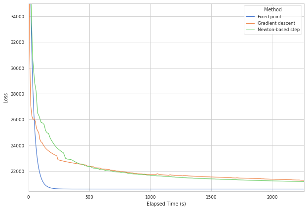
Figure 4: Value of loss Eq. 2 against elapsed time for a gradient-descent based, Newton-direction based, and fixed-point implementation of computing optimal factorizations of 2048-dimensional prefix sum matrix $\mathbf{S}$. The gradient descent and Newton direction-based methods used an Armijo step size search, and checked for existence of Cholesky factorization to verify positive-definiteness of the iterates, as suggested by [27]. The methods were initialized identically, leveraging the expression Eq. 6, a significantly better initialization for the gradient-based methods than might be obvious in the absence of this expression (e.g., initialization to $\mathbf{I}$).

To evaluate empirical usefulness of this fixed-point method, we implemented three different algorithms for computing optimal factorizations:

1. A gradient-descent-based procedure to compute the optima of Eq. 4, guaranteed to be convergent by the convexity of the problem.

2. [27, Algorithm 1], a Newton-direction-based algorithm with global convergence guarantees, hand-optimized with the structure of the problem—in particular, avoiding the need to materialize a Hessian with $n^{4}$ elements. This implementation used the default settings from [27].

3. Simply iterating the mapping $\phi$.

In all situations we tested, the fixed-point method was significantly faster than either of the other two, up to two orders of magnitude in some cases. In Fig. 4, we plot loss against time for an example of $2048\times 2048$ matrix factorization using CPUs. The methods are all similarly amenable to GPU acceleration.

Appendix F Proofs for Section 4

F.1 Proof of Proposition 4.1

Proof.

Following the analysis of Theorem C.1, Kairouz et al. [6], we introduce a hypothetical ‘unnoised’ model trajectory $\widetilde{\theta_{t}}$. Define $b_{t}:=\theta_{t}-\widetilde{\theta_{t}}$, and note that $b_{t}=-\eta\mathbf{B}_{[t,:]}\mathbf{Z}$.

We note the well-known equivalence of FTRL and gradient descent, with requilarization parameter $\lambda$ equivalent to $\frac{1}{\eta}$ (as can be seen by solving for the FTRL update). Following the standard linearization method of online convex optimization, we see:

$$\frac{1}{n}\sum_{t=1}^{n}\ell(\theta_{t};\chi_{t})-\ell(\theta^{\star};\chi_{t})\leq\frac{1}{n}\sum_{t=1}^{n}\langle\nabla_{t},\theta_{t}-\theta^{\star}\rangle=\underbrace{\frac{1}{n}\sum_{t=1}^{n}\langle\nabla_{t},\widetilde{\theta_{t}}-\theta^{\star}\rangle}_{\text{\clap{~{}A}}}+\underbrace{\frac{1}{n}\sum_{t=1}^{n}\langle\nabla_{t},\theta_{t}-\widetilde{\theta_{t}}\rangle}_{\text{\clap{~{}B}}}$$

Similarly to Kairouz et al. [6], the term A may be handled with standard online convex optimization techniques, yielding

$$\text{\clap{A}}~{}\leq\eta L^{2}+\frac{1}{2\eta n}\left(\|\theta^{\star}\|_{2}^{2}-\|\theta_{1}\|_{2}^{2}\right),$$

so we are left to evaluate the expectation of B over the noise injected by Algorithm 1. We compute:

$$\mathbb{E}\left[\frac{1}{n}\sum_{t=1}^{n}\langle\nabla_{t},\theta_{t}-\widetilde{\theta_{t}}\rangle\right] \leq\frac{1}{n}\mathbb{E}\left[\sum_{t=1}^{n}\|\nabla_{t}\|_{2}\|\theta_{t}-\widetilde{\theta_{t}}\|_{2}\right]\quad\quad$$ Cauchy-Schwartz

$$\leq\frac{L}{n}\mathbb{E}\left[\sum_{t=1}^{n}\|b_{t}\|_{2}\right]$$

$$\leq L\mathbb{E}\left[\left(\frac{1}{n}\sum_{t=1}^{n}\|b_{t}\|_{2}^{2}\right)^{1/2}\right]$$ Jensen’s inequality

$$\leq\frac{L}{\sqrt{n}}\left(\mathbb{E}\left[\sum_{t=1}^{n}\|b_{t}\|_{2}^{2}\right]\right)^{1/2}$$ Jensen again

$$=\frac{L\eta}{\sqrt{n}}\left(\mathbb{E}\left[\|\mathbf{B}\mathbf{Z}\|_{F}^{2}\right]\right)^{1/2} \text{definition of }b_{t}$$

$$=\frac{L\sigma\eta}{\sqrt{n}}\|\mathbf{B}\|_{F}$$ evaluating the expectation.

Putting together the estimates of A and B yields the result.

∎

Appendix G Visualization of Optimal Factorizations

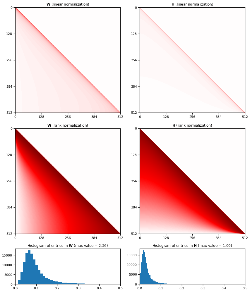
Figure 5: Visualizations of the optimal streaming matrix factorization $\mathbf{S}=\mathbf{W}\mathbf{H}$ $(\mathbf{B}=\mathbf{W},\mathbf{C}=\mathbf{H})$ for cumulative sums with $n=512$. The matrix visualizations use a color palette that maps scalars in $[0,1]$ to colors from white to dark red. The first row normalizes entries to $[0,1]$ by simply dividing all entries by 2.36 (the largest value in either matrix). This clearly shows the heavy diagonal in $\mathbf{B}$. The second row normalizes the values in each matrix by ranking them by magnitude, and then mapping the ranks to $[0,1]$ so 0 entries (the smallest) are mapped to 0.0, the median value is mapped to 0.5 (mid-red), and the largest value is mapped to 1.0 (darkest red). This visualization more clearly shows the off-diagonal structure. The final row gives a histogram of the magnitudes of the non-zero entries in each matrix.

$n$	Honaker	$(\mathbf{B}^{\star},\mathbf{C}^{\star})$	Efficient	$(h,r)$
$2^{8}=256$	$74.4$	$40.4$	$40.4$	(4, 4)
$2^{9}=512$	$116.5$	$62.0$	$62.2$	(5,4)
$2^{10}=1024$	$180.8$	$94.6$	$95.5$	(5, 5)
$2^{11}=2048$	$278.3$	$143.6$	$145.8$	(6, 5)
$2^{12}=4096$	$425.6$	$217.3$	$224.0$	(6, 6)

Table 2: Values of $\sqrt{\mathcal{L}}$ for the expected squared reconstruction error $\mathcal{L}$ defined in Eq. 2 (which implies equivalent levels of privacy). The “Efficient” column gives $\sqrt{\mathcal{L}}$ for the structured approximation $\hat{\mathbf{B}}$ of $\mathbf{B}^{\star}$ with parameters $(h,r)$ described below. When $n=2^{i}$ we choose $h+r=i$, so that the mechanism based on $\hat{\mathbf{B}}$ has memory and computation efficiency comparable to the Honaker approach.

Appendix H Computational efficiency for the matrix mechanism

Our primary goal has been to develop mechanisms with best-possible privacy vs utility tradeoffs in the streaming setting. However, the $(\mathbf{B},\mathbf{C})$ we compute are in general dense, and do not obviously admit a computationally-efficient implementation of the associated DP mechanism. In contrast, tree aggregation (including, with a careful implementation, the streaming Honaker estimator) allows implementations with only $\log(n)$ overhead; that is, each DP estimate of the $i^{th}$ partial sum can be computed in time and space $\mathcal{O}(d\log(n))$.

In this section, we demonstrate empirically that the optimal $\mathbf{B}^{\star}$ from the factorization of the prefix sum matrix $\mathbf{S}$ can be approximated by structured matrices in such a way as to be competitive with the tree-aggregation approach in terms of computation and memory, but retain the advantage of substantially improved utility. Recalling Algorithm 1, the key is to compute $\mathbf{B}_{[i,:]}\mathbf{Z}$ efficently. If $\mathbf{B}$ is arbitrary, this takes $\mathcal{O}(nd)$ operations, which is likely prohibitive.

However, having a structured matrix $\hat{\mathbf{B}}$ that allows efficient multiplication with $\mathbf{Z}$ mitigates this problem. We propose the following construction, which empirically provides a good approximation while also allowing computational efficiency. Let $\mathbf{D}^{(h)}$ denote the lower-triangular banded matrix formed by taking the first $h$ diagonals of $\mathbf{B}$, so $\mathbf{D}^{(0)}$ is the all-zero matrix, $\mathbf{D}^{(1)}$ is the main diagonal of $\mathbf{B}$, and $\mathbf{D}^{(2)}$ contains the main diagonal and one below it, etc. Let $\mathbf{U}^{(h)}\in\{0,1\}^{n\times n}$ contain a $1$ in the place of each non-zero element of $\mathbf{B}$ not captured in $\mathbf{D}^{(h)}$ and zero elsewhere, so in particular $\mathbf{B}=\mathbf{B}\odot\mathbf{U}^{(h)}+\mathbf{D}^{(h)}$ where $\odot$ is elementwise multiplication. Then, we propose the representation

$$\hat{\mathbf{B}}=\big{(}\mathbf{L}\mathbf{R}^{\top}\big{)}\odot\mathbf{U}^{(h)}+\mathbf{D}^{(h)},$$

where $\mathbf{L},\mathbf{R}\in\mathbb{R}^{n\times r}$. Finding a low-rank factorization $\mathbf{L}\mathbf{R}^{\top}$ which minimizes $\|\hat{\mathbf{B}}-\mathbf{B}\|_{F}^{2}$ can be cast as a matrix completion problem, as we only care about approximating with $\mathbf{L}\mathbf{R}^{\top}$ the entries of $\mathbf{B}$ selected by $\mathbf{U}^{(h)}$. For these experiments we used an alternating least squares solver with a regularization penalty of $10^{-6}$ on $\|\mathbf{L}\|^{2}_{F}+\|\mathbf{R}\|^{2}_{F}$ [63, 64, 65]. Given such a representation, the cost of computing $\hat{\mathbf{B}}_{[i,:]}\mathbf{Z}$ is $\mathcal{O}((h+r)d)$: we maintain accumulators $\boldsymbol{\beta}$ such that

$$(\mathbf{L}\boldsymbol{\beta})_{[i,:]}=\big{(}(\mathbf{L}\mathbf{R}^{\top}\odot\mathbf{U}^{(h)})\mathbf{Z}\big{)}_{[i,:]},$$

and $\boldsymbol{\beta}$ can be updated in time $rd$ on each step. Then, Finally, $(\mathbf{D}^{(h)}\mathbf{Z})_{[i,:]}$ can be computed in time $hd$. Algorithm 3 makes this algorithm explicit.

Columns 3 and 4 in Table 2 shows empirically that this approximation recovers almost all of the accuracy improvement of $(\mathbf{B}^{\star},\mathbf{C}^{\star})$ at comparable computational efficiency to tree aggregation with the Honaker estimator (that is, we choose $h+r=\log_{2}(n)$). While a paired $\mathbf{C}$ is not used directly in computing the private estimates, it is necessary in order to compute the loss $\mathcal{L}$ defined in Eq. 2, as well as to appropriately calibrate the noise to achieve a DP guarantee (see Theorem 3.1). For these purposes an optimal $\mathbf{C}_{\hat{\mathbf{B}}}$ can be found analogous to Eq. 3 as $\mathbf{C}_{\hat{\mathbf{B}}}=\hat{\mathbf{B}}^{-1}\mathbf{S}$.

Algorithm 3 An efficient implementation (executed by the trusted curator)

1:# Iterations and matrices/vectors are zero indexed (unlike elsewhere)

2:Parameters:

3:      Matrix $\mathbf{D}^{(h)}$ containing $h\in\{0,\dots,n\}$ diagonals from $\mathbf{B}$

4:      Matrices $\mathbf{L},\mathbf{R}\in\mathbb{R}^{n\times r}$

5:      Noise matrix $\mathbf{Z}\in\mathbb{R}^{n\times d}$

6:      Observations $\mathbf{G}\in\mathbb{R}^{n\times d}$

7:$\boldsymbol{\beta}:=\mathbf{0}\in\mathbb{R}^{r\times d}$          # Buffer for relevant part of $\mathbf{R}^{\top}\mathbf{Z}$.

8:$\mathbf{s}:=0\in\mathbb{R}^{d}$          # Accumulator for prefix sum

9:for $i$ in $1,\dots,n$ do

10:     $\mathbf{s}\mathrel{+}=\mathbf{G}_{[i,:]}$          # Maintain the un-noised cumulative sum

11:     $\mathbf{y}:=0\in\mathbb{R}^{d}$          # Accumulator for total noise in $i$th prefix sum

12:     for $k$ in $0,\dots,\min(i,h-1)$ do          # Handle $h$ diagonals directly; No-op if $h=0$

13:         $\mathbf{y}\mathrel{+}=\mathbf{D}^{(h)}_{[i,i-k]}\mathbf{Z}_{[i-k,:]}$          # $hd$ multiplies      

14:     if $i\geq h$ then          # Compute the low-rank portion

15:         $i^{\prime}\leftarrow i-h$

16:         $\boldsymbol{\beta}\mathrel{+}=\mathbf{R}^{\top}_{[i^{\prime},:]}\mathbf{Z}_{[i^{\prime},:]}$          # $rd$ multiplies

17:         $\mathbf{y}\mathrel{+}=\mathbf{L}_{[i,:]}\boldsymbol{\beta}$          # $rd$ multiplies      

18:     Release $\mathbf{s}+\mathbf{y}$          # A DP estimate of $\sum_{t=1}^{i}\mathbf{G}_{[t,:]}$

Appendix I Experiment Details

Mechanism implementation

Though Appendix H shows that time- and space-bounded approximations to our optimal factorizations are possible, for our experimental results we followed Algorithm 1 and implemented the straightforward version of our mechanism. That is, we leverage the expression

$$\mathbf{B}\left(\mathbf{C}\mathbf{G}+\mathbf{Z}\right)=\mathbf{A}\mathbf{G}+\mathbf{B}\mathbf{Z},$$

for $\mathbf{A}=\mathbf{B}\mathbf{C}$, where $\mathbf{A}$ represents the linear operator we are interested in estimating. By introducing a seed to the generation of the noise vector $\mathbf{Z}$, the appropriate noise vector $(\mathbf{B}\mathbf{Z})_{[i,:]}$ can simply be computed afresh for each iteration of training (or round in the federated setting). The linear operators $\mathbf{A}$ in which we are interested admit efficient implementations; e.g., gradient descent with momentum can be implemented with a single buffer, representing the current state of the model. The computation of $\mathbf{B}\mathbf{Z}$ is therefore the dominant component in the above.

We normalized all of our factorizations to have sensitivity exactly 1 in the single-pass setting.

Integration with federated learning

We implemented these mechanisms via the DPQuery interface in TensorFlow-Privacy [66], which integrates naturally with tff.aggregators, the aggregators library of TensorFlow-Federated. We were therefore able to reuse precisely the same code for training as [67], simply swapping in our matrix-factorization-based aggregators as an argument to TFF’s tff.learning.build_federated_averaging_process function. In conjunction with this paper, we are in the process of open-sourcing the code to reproduce our experiments. TFF’s distributed C++ runtime, equipped with one machine for every 10 clients per round and low-priority CPU resources, enabled our experiment grids (including evaluation) to finish in approximately 1 day.

Stackoverflow settings

The preprocessing of our data, in addition to model architecture as well as the settings of various task-specific hyperparameters like the maximum number of examples processed per-client, we share with [6].

Test accuracy details

Test accuracies (excluding predictions on out-of-vocabulary and end-of-sentence tokens) plotted against $\varepsilon$ values associated to $\delta=10^{-6}$ for various instantiations of the mechanisms we tested can be found in Fig. 3. This figure was generated with a sweep over client and server learning rates, with grids chosen via in the heatmap for FedAvgM in Figure 2 of [51], as well as a sweep over server momentum values. The noise multiplier settings were chosen with a simple calculation, based on the reported noise multipliers for StackOverflow NWP in [6]. In particular, by explicitly calculating the sensitivity of the binary tree (as in Theorem 4.1 of [6]), one can normalize the noise multipliers to be equivalent between the two settings. In the process of testing our code, we verified that we observed similar results to those claimed there under this normalization. The smallest noise multiplier in our setting corresponds to the largest $\varepsilon$ in figure 2(a) of [6], though our plots are not exactly comparable to theirs due to the different number of rounds in the two experimental setups. We calculate our $\varepsilon$ values by simply measuring the privacy cost of the appropriate high-dimensional Gaussian query, by Theorem 4.1. The grid we swept over can be found in Table 3.

The error bars in Figs. 3 and 3 were generated by first filtering down to runs which did not diverge from repeated runs with 10 seeds (at least 7 converged for each setting in Fig. 3, at least 8 for each setting in Fig. 3), then computing the empirical standard deviation. A similar process was used for Fig. 6.

Evaluation accuracy details

During training, we monitored performance on an evaluation set consisting of 10,000 sentences from outside of the training and test sets. We plot this evaluation accuracy for the final portion of training our learning-rate schedule and momentum matrices in Fig. 6.

Additional figures

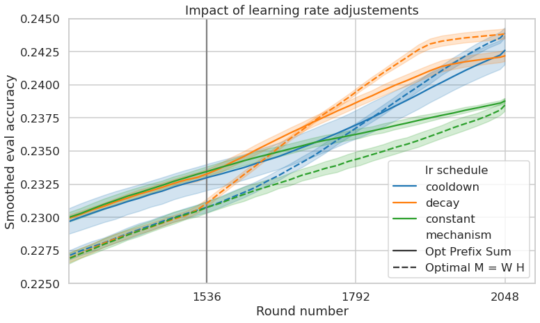
Figure 6: Smoothed validation accuracy over the final 748 rounds at $\varepsilon=18.9,\delta=10^{-6}$, comparing momentum and learning rate decay implemented as postprocessing operations to the prefix-sum mechanism versus capturing these operations in the mechanism itself (see Section 4). Vertical line represents the start of the decay schedule.

We note that Fig. 6 demonstrates a consistent artifact we witnessed in training these models: the momentum matrix factorization performs worse than the prefix-sum matrix during the body of training, but catches up and overtakes towards the end of the training procedure. We hypothesize this to be an artifact of the way these mechanisms distribute variance on the operator residuals, and consider it an interesting pointer for future mechanism design, while noting that it implies the matrix factorizations are significantly tuned to the number of iterations for which they are designed.

Hyperparameter settings

The parameter settings for the various figures in the main body and appendix can be found below.

Table 3: Grids used in initial search for Fig. 3.

Parameter	Grid values
Client learning rate	[0.5, 1.0]
Server learning rate	[0.25, 0.5, 1.0, 2.0]
Server momentum	[0.0, 0.9, 0.95]
Noise multiplier	[0.341, 0.682, 1.364, 2.728, 5.456]

Table 4: Hyperparameter settings for Fig. 3.

Mechanism	$\varepsilon$	(Server LR, Client LR, Server momentum)
Honaker Full	18.9	$(0.5,1.,0.95)$
	8.2	$(0.25,1.,0.95)$
	3.7	$(0.25,1.,0.9)$
	1.7	$(0.25,0.5,0.9)$
	0.8	$(0.25,0.5,0.0)$
Honaker Online	18.9	$(0.25,1.,0.95)$
	8.2	$(0.25,1.,0.9)$
	3.7	$(0.25,0.5,0.9)$
	1.7	$(0.25,1.,0.0)$
	0.8	$(0.25,0.5,0.0)$
Opt Prefix Sum	18.9	$(0.5,1.,0.95)$
	8.2	$(0.25,0.5,0.95)$
	3.7	$(0.25,1.,0.9)$
	1.7	$(0.25,0.5,0.9)$
	0.8	$(0.5,0.5,0.0)$
Optimal M = B C	18.9	$(1.,1.,0.9)$
	8.2	$(0.25,1.,0.95)$
	3.7	$(0.25,0.5,0.9)$
	1.7	$(0.25,0.5,0.9)$
	0.8	$(0.5,0.5,0.0)$

For Fig. 3, the parameter settings differed based on the mechanisms explored. Constant LR schedules used the same settings as $\varepsilon=18.9$ in Table 4. For the exploration of learning rate decay schedules, a server learning rate of $0.5$, client learning rate of $1.0$, and server momentum of $0.95$ were shared. The plot Fig. 6 was generated from the same set of experiments.

Appendix J Background on Differential Privacy

In this paper we operate with the “replace with zero” variant of differential privacy [6, Defn. 2.1], sated below for completeness purposes.

Definition J.1 (Differential privacy).

Let $\mathcal{D}$ be the domain of data records, $\bot\not\in\mathcal{D}$ be a special element, and let $\widehat{\mathcal{D}}=\mathcal{D}\cup\{\bot\}$ be the extended domain. A randomized algorithm $\mathcal{A}:\widehat{\mathcal{D}}^{n}\to\mathcal{S}$ is $(\varepsilon,\delta)$-differentially private if for any data set $D\in\widehat{\mathcal{D}}^{n}$ and any neighbor $D^{\prime}\in\widehat{\mathcal{D}}^{n}$ (formed from $D$ by replacing one record with $\bot$), and for any event $S\in\mathcal{S}$, we have

$$\Pr[\mathcal{A}(D)\in S] \leq e^{\varepsilon}\cdot\Pr[\mathcal{A}(D^{\prime})\in S]+\delta,\ \ \text{and}$$

$$\Pr[\mathcal{A}(D^{\prime})\in S] \leq e^{\varepsilon}\cdot\Pr[\mathcal{A}(D)\in S]+\delta,$$

where the probability is over the randomness of $\mathcal{A}$.

In our algorithms, we would treat $\bot$ specially, and assume it corresponds to the all-zeros vector of appropriate dimensions. This definition extends naturally to other variants like Renyi differential privacy (RDP) [35], and zero Concentrated Differential Privacy (zCDP). For completeness purposes we provide the definition of zCDP we primarily use in the paper.

Definition J.2 (zero concentrated differential privacy).

Analogous to the definitiion of $(\varepsilon,\delta)$-differential privacy in Definition J.1, a randomized algorithm $\mathcal{A}$ is $\rho$-zCDP if the condition on $\mathcal{A}(D)$ and $\mathcal{A}(D^{\prime})$ in Definition J.1 are replaced with the following:

$$\frac{1}{\alpha-1}\log\mathbb{E}_{s\sim\mathcal{A}(D)}{\left(\frac{\Pr\left[\mathcal{A}(D)=s\right]}{\Pr\left[\mathcal{A}(D^{\prime})=s\right]}\right)^{\alpha}} \leq\rho\alpha,\ \ \text{and}$$

$$\frac{1}{\alpha-1}\log\mathbb{E}_{s\sim\mathcal{A}(D^{\prime})}{\left(\frac{\Pr\left[\mathcal{A}(D^{\prime})=s\right]}{\Pr\left[\mathcal{A}(D)=s\right]}\right)^{\alpha}} \leq\rho\alpha.$$

References

- Li et al. [2015] Chao Li, Gerome Miklau, Michael Hay, Andrew Mcgregor, and Vibhor Rastogi. The matrix mechanism: optimizing linear counting queries under differential privacy. The VLDB Journal, 24:757–781, 2015.
- Dwork et al. [2006a] Cynthia Dwork, Frank McSherry, Kobbi Nissim, and Adam Smith. Calibrating noise to sensitivity in private data analysis. In Shai Halevi and Tal Rabin, editors, Theory of Cryptography, pages 265–284, Berlin, Heidelberg, 2006a. Springer Berlin Heidelberg. ISBN 978-3-540-32732-5.
- Chan et al. [2011] T.-H. Hubert Chan, Elaine Shi, and Dawn Song. Private and continual release of statistics. ACM Trans. on Information Systems Security, 14(3):26:1–26:24, November 2011.
- Dwork et al. [2010] Cynthia Dwork, Moni Naor, Toniann Pitassi, and Guy N. Rothblum. Differential privacy under continual observation. In Proc. of the Forty-Second ACM Symp. on Theory of Computing (STOC’10), pages 715–724, 2010.
- Jain et al. [2012] Prateek Jain, Pravesh Kothari, and Abhradeep Thakurta. Differentially private online learning. In Proc. of the 25th Annual Conf. on Learning Theory (COLT), volume 23, pages 24.1–24.34, June 2012.
- Kairouz et al. [2021] Peter Kairouz, Brendan McMahan, Shuang Song, Om Thakkar, Abhradeep Thakurta, and Zheng Xu. Practical and private (deep) learning without sampling or shuffling. In ICML, 2021.
- Smith and Thakurta [2013] Adam Smith and Abhradeep Thakurta. (nearly) optimal algorithms for private online learning in full-information and bandit settings. In Advances in Neural Information Processing Systems, pages 2733–2741, 2013.
- Jain et al. [2021] Palak Jain, Sofya Raskhodnikova, Satchit Sivakumar, and Adam D. Smith. The price of differential privacy under continual observation. ArXiv CoRR, abs/2112.00828, 2021. URL https://arxiv.org/abs/2112.00828.
- Agarwal and Singh [2017] Naman Agarwal and Karan Singh. The price of differential privacy for online learning. In International Conference on Machine Learning, pages 32–40. PMLR, 2017.
- Dwork et al. [2014] Cynthia Dwork, Kunal Talwar, Abhradeep Thakurta, and Li Zhang. Analyze gauss: optimal bounds for privacy-preserving principal component analysis. In Proceedings of the forty-sixth annual ACM symposium on Theory of computing, pages 11–20, 2014.
- Cormode et al. [2019] Graham Cormode, Tejas Kulkarni, and Divesh Srivastava. Answering range queries under local differential privacy. Proceedings of the VLDB Endowment, 12(10):1126–1138, 2019.
- Cardoso and Rogers [2021] Adrian Rivera Cardoso and Ryan Rogers. Differentially private histograms under continual observation: Streaming selection into the unknown. CoRR, abs/2103.16787, 2021. URL https://arxiv.org/abs/2103.16787.
- Smith et al. [2017] Adam Smith, Abhradeep Thakurta, and Jalaj Upadhyay. Is interaction necessary for distributed private learning? In 2017 IEEE Symposium on Security and Privacy (SP), pages 58–77. IEEE, 2017.
- Thakurta and Smith [2013] Abhradeep Guha Thakurta and Adam Smith. (nearly) optimal algorithms for private online learning in full-information and bandit settings. In C.J. Burges, L. Bottou, M. Welling, Z. Ghahramani, and K.Q. Weinberger, editors, Advances in Neural Information Processing Systems, volume 26. Curran Associates, Inc., 2013. URL https://proceedings.neurips.cc/paper/2013/file/c850371fda6892fbfd1c5a5b457e5777-Paper.pdf.
- Song et al. [2013] Shuang Song, Kamalika Chaudhuri, and Anand D Sarwate. Stochastic gradient descent with differentially private updates. In 2013 IEEE Global Conference on Signal and Information Processing, pages 245–248. IEEE, 2013.
- Bassily et al. [2014] Raef Bassily, Adam Smith, and Abhradeep Thakurta. Private empirical risk minimization: Efficient algorithms and tight error bounds. In Proc. of the 2014 IEEE 55th Annual Symp. on Foundations of Computer Science (FOCS), pages 464–473, 2014.
- Abadi et al. [2016] Martin Abadi, Andy Chu, Ian Goodfellow, H. Brendan McMahan, Ilya Mironov, Kunal Talwar, and Li Zhang. Deep learning with differential privacy. Proceedings of the 2016 ACM SIGSAC Conference on Computer and Communications Security, Oct 2016. doi: 10.1145/2976749.2978318. URL http://dx.doi.org/10.1145/2976749.2978318.
- Tyagi et al. [2017] Nirvan Tyagi, Yossi Gilad, Derek Leung, Matei Zaharia, and Nickolai Zeldovich. Stadium: A distributed metadata-private messaging system. In Proceedings of the 26th Symposium on Operating Systems Principles, pages 423–440, 2017.
- Úlfar Erlingsson et al. [2019] Úlfar Erlingsson, Ilya Mironov, Ananth Raghunathan, and Shuang Song. That which we call private, 2019.
- Joseph et al. [2018] Matthew Joseph, Aaron Roth, Jonathan Ullman, and Bo Waggoner. Local differential privacy for evolving data. Advances in Neural Information Processing Systems, 31, 2018.
- Apple [2017] Differential Privacy Team Apple. Learning with privacy at scale, 2017.
- Honaker [2015] James Honaker. Efficient use of differentially private binary trees. Theory and Practice of Differential Privacy (TPDP 2015), London, UK, 2015.
- McMahan and Streeter [2010] H Brendan McMahan and Matthew Streeter. Adaptive bound optimization for online convex optimization. arXiv preprint arXiv:1002.4908, 2010.
- McMahan [2011] Brendan McMahan. Follow-the-regularized-leader and mirror descent: Equivalence theorems and l1 regularization. In Proceedings of the Fourteenth International Conference on Artificial Intelligence and Statistics, pages 525–533, 2011.
- Duchi et al. [2011] John Duchi, Elad Hazan, and Yoram Singer. Adaptive subgradient methods for online learning and stochastic optimization. Journal of machine learning research, 12(7), 2011.
- Hardt and Talwar [2010] Moritz Hardt and Kunal Talwar. On the geometry of differential privacy. In STOC, 2010.
- Yuan et al. [2016] Ganzhao Yuan, Yin Yang, Zhenjie Zhang, and Zhifeng Hao. Optimal linear aggregate query processing under approximate differential privacy. CoRR, abs/1602.04302, 2016. URL http://arxiv.org/abs/1602.04302.
- McKenna et al. [2021] Ryan McKenna, Gerome Miklau, Michael Hay, and Ashwin Machanavajjhala. HDMM: optimizing error of high-dimensional statistical queries under differential privacy. CoRR, abs/2106.12118, 2021. URL https://arxiv.org/abs/2106.12118.
- Edmonds et al. [2020] Alexander Edmonds, Aleksandar Nikolov, and Jonathan Ullman. The Power of Factorization Mechanisms in Local and Central Differential Privacy, page 425–438. Association for Computing Machinery, New York, NY, USA, 2020. ISBN 9781450369794. URL https://doi.org/10.1145/3357713.3384297.
- Fichtenberger et al. [2022] Hendrik Fichtenberger, Monika Henzinger, and Jalaj Upadhyay. Constant matters: Fine-grained complexity of differentially private continual observation, 2022. URL https://arxiv.org/abs/2202.11205.
- Dwork et al. [2006b] Cynthia Dwork, Frank McSherry, Kobbi Nissim, and Adam Smith. Calibrating noise to sensitivity in private data analysis. In Proc. of the Third Conf. on Theory of Cryptography (TCC), pages 265–284, 2006b. URL http://dx.doi.org/10.1007/11681878_14.
- Dwork et al. [2006c] Cynthia Dwork, Krishnaram Kenthapadi, Frank McSherry, Ilya Mironov, and Moni Naor. Our data, ourselves: Privacy via distributed noise generation. In Advances in Cryptology—EUROCRYPT, pages 486–503, 2006c.
- Bun and Steinke [2016] Mark Bun and Thomas Steinke. Concentrated differential privacy: Simplifications, extensions, and lower bounds. In Theory of Cryptography Conference, pages 635–658. Springer, 2016.
- Dwork and Rothblum [2016] Cynthia Dwork and Guy N. Rothblum. Concentrated differential privacy. CoRR, abs/1603.01887, 2016.
- Mironov [2017] Ilya Mironov. Rényi differential privacy. In 2017 IEEE 30th Computer Security Foundations Symposium (CSF), pages 263–275. IEEE, 2017.
- Dong et al. [2019] Jinshuo Dong, Aaron Roth, and Weijie J. Su. Gaussian differential privacy. CoRR, abs/1905.02383, 2019. URL http://arxiv.org/abs/1905.02383.
- Koskela et al. [2021] Antti Koskela, Joonas Jälkö, Lukas Prediger, and Antti Honkela. Tight differential privacy for discrete-valued mechanisms and for the subsampled gaussian mechanism using fft. In International Conference on Artificial Intelligence and Statistics, pages 3358–3366. PMLR, 2021.
- Campbell and Meyer [1979] S. L. Campbell and C. D. Meyer. Generalized inverses of linear transformations / S. L. Campbell, C. D. Meyer. Pitman London ; San Francisco, 1979. ISBN 0273084224.
- Jozsa [1994] Richard Jozsa. Fidelity for mixed quantum states. Journal of Modern Optics, 41(12):2315–2323, 1994. doi: 10.1080/09500349414552171. URL https://doi.org/10.1080/09500349414552171.
- Liang et al. [2019] Yeong-Cherng Liang, Yu-Hao Yeh, Paulo E M F Mendonça, Run Yan Teh, Margaret D Reid, and Peter D Drummond. Quantum fidelity measures for mixed states. Reports on Progress in Physics, 82(7):076001, jun 2019. doi: 10.1088/1361-6633/ab1ca4. URL https://doi.org/10.1088/1361-6633/ab1ca4.
- Lawson and Lim [2001] Jimmie D. Lawson and Yongdo Lim. The geometric mean, matrices, metrics, and more. The American Mathematical Monthly, 108(9):797–812, 2001. doi: 10.1080/00029890.2001.11919815. URL https://doi.org/10.1080/00029890.2001.11919815.
- Kubo and Ando [1979] Fumio Kubo and Tsuyoshi Ando. Means of positive linear operators. Mathematische Annalen, 246:205–224, 1979. URL http://eudml.org/doc/163339.
- Polyak [1964] B.T. Polyak. Some methods of speeding up the convergence of iteration methods. USSR Computational Mathematics and Mathematical Physics, 4(5):1–17, 1964. ISSN 0041-5553.
- Hard et al. [2018] Andrew Hard, Kanishka Rao, Rajiv Mathews, Françoise Beaufays, Sean Augenstein, Hubert Eichner, Chloé Kiddon, and Daniel Ramage. Federated learning for mobile keyboard prediction. CoRR, abs/1811.03604, 2018. URL http://arxiv.org/abs/1811.03604.
- Ramaswamy et al. [2020] Swaroop Ramaswamy, Om Thakkar, Rajiv Mathews, Galen Andrew, H. Brendan McMahan, and Françoise Beaufays. Training production language models without memorizing user data, 2020.
- Carlini et al. [2019] Nicholas Carlini, Chang Liu, Úlfar Erlingsson, Jernej Kos, and Dawn Song. The secret sharer: Evaluating and testing unintended memorization in neural networks. In Proceedings of the 28th USENIX Conference on Security Symposium, SEC’19, page 267–284, USA, 2019. USENIX Association. ISBN 9781939133069.
- Song and Shmatikov [2019] Congzheng Song and Vitaly Shmatikov. Auditing data provenance in text-generation models. In Proceedings of the 25th ACM SIGKDD International Conference on Knowledge Discovery & Data Mining, pages 196–206, 2019.
- Carlini et al. [2021] Nicholas Carlini, Florian Tramèr, Eric Wallace, Matthew Jagielski, Ariel Herbert-Voss, Katherine Lee, Adam Roberts, Tom Brown, Dawn Song, Úlfar Erlingsson, Alina Oprea, and Colin Raffel. Extracting training data from large language models. In 30th USENIX Security Symposium (USENIX Security 21), pages 2633–2650. USENIX Association, August 2021. ISBN 978-1-939133-24-3. URL https://www.usenix.org/conference/usenixsecurity21/presentation/carlini-extracting.
- McMahan et al. [2017a] H Brendan McMahan, Daniel Ramage, Kunal Talwar, and Li Zhang. Learning differentially private recurrent language models. arXiv preprint arXiv:1710.06963, 2017a.
- McMahan et al. [2017b] H. Brendan McMahan, Eider Moore, Daniel Ramage, Seth Hampson, and Blaise Agüera y Arcas. Communication-efficient learning of deep networks from decentralized data. In Proceedings of the 20th International Conference on Artificial Intelligence and Statistics, AISTATS 2017, 20-22 April 2017, Fort Lauderdale, FL, USA, pages 1273–1282, 2017b. URL http://proceedings.mlr.press/v54/mcmahan17a.html.
- Reddi et al. [2020] Sashank J. Reddi, Zachary Charles, Manzil Zaheer, Zachary Garrett, Keith Rush, Jakub Konečný, Sanjiv Kumar, and H. Brendan McMahan. Adaptive federated optimization. CoRR, abs/2003.00295, 2020. URL https://arxiv.org/abs/2003.00295.
- Ingerman and Ostrowski [2019] Alex Ingerman and Krzysztof Ostrowski. Introducing tensorflow federated, Mar 2019. URL https://blog.tensorflow.org/2019/03/introducing-tensorflow-federated.html.
- Charles et al. [2021] Zachary Charles, Zachary Garrett, Zhouyuan Huo, Sergei Shmulyian, and Virginia Smith. On large-cohort training for federated learning. In A. Beygelzimer, Y. Dauphin, P. Liang, and J. Wortman Vaughan, editors, Advances in Neural Information Processing Systems, 2021. URL https://openreview.net/forum?id=Kb26p7chwhf.
- Zhu et al. [2022] Chen Zhu, Zheng Xu, Mingqing Chen, Jakub Konečný, Andrew Hard, and Tom Goldstein. Diurnal or nocturnal? federated learning of multi-branch networks from periodically shifting distributions. In International Conference on Learning Representations, 2022.
- Singhal et al. [2021] Karan Singhal, Hakim Sidahmed, Zachary Garrett, Shanshan Wu, Keith Rush, and Sushant Prakash. Federated reconstruction: Partially local federated learning. CoRR, abs/2102.03448, 2021. URL https://arxiv.org/abs/2102.03448.
- Vadhan [2017] Salil Vadhan. The complexity of differential privacy. In Tutorials on the Foundations of Cryptography, pages 347–450. Springer, 2017.
- Horn and Johnson [1990] Roger A. Horn and Charles R. Johnson. Matrix Analysis. Cambridge University Press, 1990. ISBN 0521386322. URL http://www.amazon.com/Matrix-Analysis-Roger-Horn/dp/0521386322%3FSubscriptionId%3D192BW6DQ43CK9FN0ZGG2%26tag%3Dws%26linkCode%3Dxm2%26camp%3D2025%26creative%3D165953%26creativeASIN%3D0521386322.
- Steinke [2022] Thomas Steinke. Composition of differential privacy &; privacy amplification by subsampling, 2022. URL https://arxiv.org/abs/2210.00597.
- Dwork and Roth [2014] Cynthia Dwork and Aaron Roth. The algorithmic foundations of differential privacy. Foundations and Trends in Theoretical Computer Science, 9(3–4):211–407, 2014.
- Boyd and Vandenberghe [2004] Stephen Boyd and Lieven Vandenberghe. Convex Optimization. Cambridge University Press, March 2004. ISBN 0521833787. URL http://www.amazon.com/exec/obidos/redirect?tag=citeulike-20&path=ASIN/0521833787.
- Bertsekas [1999] D.P. Bertsekas. Nonlinear Programming. Athena Scientific, 1999.
- Merikoski and Kumar [2004] Jorma Merikoski and Ravinder Kumar. Inequalities for spreads of matrix sums and products. Applied Mathematics E-Notes [electronic only], 4, 01 2004.
- Srebro et al. [2005] Nathan Srebro, Jason Rennie, and Tommi Jaakkola. Maximum-margin matrix factorization. In L. Saul, Y. Weiss, and L. Bottou, editors, Advances in Neural Information Processing Systems, volume 17. MIT Press, 2005. URL https://proceedings.neurips.cc/paper/2004/file/e0688d13958a19e087e123148555e4b4-Paper.pdf.
- Koren et al. [2009] Yehuda Koren, Robert Bell, and Chris Volinsky. Matrix factorization techniques for recommender systems. Computer, 42(8), 2009. ISSN 0018-9162. doi: 10.1109/MC.2009.263. URL https://doi.org/10.1109/MC.2009.263.
- Jain et al. [2013] Prateek Jain, Praneeth Netrapalli, and Sujay Sanghavi. Low-rank matrix completion using alternating minimization. In Proceedings of the Forty-Fifth Annual ACM Symposium on Theory of Computing (STOC). Association for Computing Machinery, 2013. ISBN 9781450320290.
- [66] Google. Tensorflow-privacy. https://github.com/tensorflow/privacy, year=2019.
- Thakkar et al. [2019] Om Thakkar, Galen Andrew, and H Brendan McMahan. Differentially private learning with adaptive clipping. arXiv preprint arXiv:1905.03871, 2019.