Cost-Efficient Distributed Learning via Combinatorial Multi-Armed Bandits

Abstract

We consider the distributed stochastic gradient descent problem, where a main node distributes gradient calculations among $n$ workers. By assigning tasks to all the workers and waiting only for the $k$ fastest ones, the main node can trade-off the algorithm’s error with its runtime by gradually increasing $k$ as the algorithm evolves. However, this strategy, referred to as adaptive $k$-sync, neglects the cost of unused computations and of communicating models to workers that reveal a straggling behavior. We propose a cost-efficient scheme that assigns tasks only to $k$ workers, and gradually increases $k$. We introduce the use of a combinatorial multi-armed bandit model to learn which workers are the fastest while assigning gradient calculations. Assuming workers with exponentially distributed response times parameterized by different means, we give empirical and theoretical guarantees on the regret of our strategy, i.e., the extra time spent to learn the mean response times of the workers. Furthermore, we propose and analyze a strategy applicable to a large class of response time distributions. Compared to adaptive $k$-sync, our scheme achieves significantly lower errors with the same computational efforts and less downlink communication while being inferior in terms of speed.

I Introduction

We consider a distributed machine learning setting, in which a central entity, referred to as the main node, possesses a large amount of data on which it wants to run a machine learning algorithm. To speed up the computations, the main node distributes the computation tasks to several worker machines. The workers compute smaller tasks in parallel and send back their results to the main node, which then aggregates the results to obtain the desired result of the large computation. A naive distribution of the tasks to the workers suffers from the presence of stragglers, i.e., slow or even unresponsive workers [1, 2].

The negative effect of stragglers can be mitigated by assigning redundant computations to the workers and ignoring the response of the slowest ones, e.g., [3, 4]. However, in gradient descent algorithms, assigning redundant tasks to the workers can be avoided when a (good) estimate of the gradient loss function is sufficient. On a high level, gradient descent is an iterative algorithm requiring the main node to compute the gradient of a loss function at every iteration based on the current model. Simply ignoring the stragglers is equivalent to stochastic gradient descent (SGD) [5, 6], which advocates computing an estimate of the gradient of the loss function at every iteration [2, 7]. As a result, SGD trades-off the time spent per iteration with the total number of iterations for convergence, or until a desired result is reached. The authors of [8] show that for distributed SGD algorithms, it is faster for the main node to assign tasks to all the workers, but wait for only a small subset of the workers to return their results. In the strategy proposed in [8], called adaptive $k$-sync, in order to improve the convergence speed, the main node increases the number of workers it waits for as the algorithm evolves in iterations. Despite reducing the run-time of the algorithm, i.e., the total time needed to reach the desired result, this strategy requires the main node to transmit the current model to all available workers and pay for all computational resources while only using the computations of the fastest ones.

In this work, we take into account the cost of employing workers and for transferring the current model to the workers. In contrast to [8], we propose a communication- and computation-efficient scheme that distributes tasks only to the fastest workers and waits for the completion of all their computations. However, in practice, the main node does not know in advance which workers are the fastest. To this end, we introduce the use of a stochastic MAB framework to learn the speed of the workers while efficiently assigning them computational tasks. Stochastic MABs, introduced in [9], are iterative algorithms initially designed to maximize the gain of a user gambling with multiple slot machines, termed “armed bandits”. At each iteration, the user is allowed to pull one arm from the available set of armed bandits. Each arm pull yields a random reward following a known distribution with an unknown mean. The user wants to design a strategy to learn the expected reward of the arms while maximizing the accumulated rewards. Stochastic combinatorial were introduced in [10] and model the behavior when a user seeks to find a combination of arms that reveals the best overall expected reward.

Following the literature on distributed computing [11, 3], we model the response times of the workers by independent and exponentially distributed random variables. We additionally assume that the workers are heterogeneous, i.e., have different mean response times. To apply MABs to distributed computing, we model the rewards by the response times and aim to minimize the rewards. Under this model, we show that compared to adaptive $k$-sync, using a MAB to learn the mean response times of the workers on the fly cuts the average cost (reflected by the total number of worker employments) but comes at the expense of significantly increasing the total run-time of the algorithm.

I-A Related Work

I-A1 Distributed Gradient Descent

Assigning redundant tasks to the workers and running distributed gradient descent is known as gradient coding [4, 12, 13, 14, 15, 16]. Approximate gradient coding is introduced to reduce the required redundancy and run SGD in the presence of stragglers [17, 18, 19, 20, 21, 22, 23, 24]. The schemes in [15, 16] use redundancy but no coding to avoid encoding/decoding overheads. However, assigning redundant computations to the workers increases the computation time spent per worker and may slow down the overall computation process. Thus, [7, 2, 8] advocate running distributed SGD without redundant task assignment to the workers. In [7], the convergence speed of the algorithm is analyzed in terms of the wall-clock time rather than the number of iterations. It is assumed that the main node waits for $k$ out of $n$ workers and ignores the rest. The authors of [8] show that gradually increasing $k$, i.e., gradually decreasing the number of tolerated stragglers as the algorithm evolves, increases the convergence speed of the algorithm. In this work, we consider a similar analysis to the one in [8]; however, instead of assigning tasks to all the workers and ignoring the stragglers, we require the main node to only employ (assign tasks to) the required amount of workers. To learn the speed of the workers and choose the fastest ones, we use ideas from the literature on MABs.

I-A2 MABs

Since their introduction in [9], MABs have been extensively studied for decision-making under uncertainty. A MAB strategy is evaluated by its regret defined as the difference between the actual cumulative reward and the one that could be achieved should the user know the expected reward of the arms a priori. The works of [25, 26] introduced the use of upper confidence bounds based on previous rewards to decide which arm to pull at each iteration. Those schemes are said to be asymptotically optimal since their regret becomes negligible as the number of iterations goes to infinity. In [27], the regret of a UCB algorithm is bounded for a finite number of iterations. Subsequent research aims to improve on this by introducing variants of UCBs, e.g., KL-UCB [28, 29] which is based on Kullback-Leibler (KL)-divergence. While most of the works assume a finite support for the reward, MABs with unbounded rewards were studied in [28, 29, 30, 31], where in the latter the variance factor is assumed to be known. In the class of CMABs, the user is allowed to pull multiple arms with different characteristics at each iteration. The authors of [10] extended the asymptotically efficient allocation rules of [25] to a CMAB scenario. General frameworks for the CMAB with bounded reward functions are investigated in [32, 33, 34, 35]. The analysis in [36, 37] for linear reward functions with finite support is an extension of the classical UCB strategy, and comes closest to our work.

I-B Contributions and Outline

After a description of the system model in Section II, we introduce in Section III a CMAB model based on lower confidence bounds to reduce the cost of distributed gradient descent, measured in terms of the number of worker employments, whether the results of the corresponding computations carried out by the workers are used by the main node or not. Our cost-efficient policy increases the number of employed workers as the algorithm evolves. In Section IV, we introduce and theoretically analyze an LCB that is particularly suited to exponential distributions and easy to compute for the master. To improve the performance of our CMAB, we investigate in Section V an LCB that is based on KL-divergence, and generalizes to all bounded reward distributions and those belonging to the canonical exponential family. This comes at the expense of a higher computational complexity for the main node. In Section VI, we provide simulation results for linear regression to underline our theoretical findings. Section VII concludes the paper.

II System Model and Preliminaries

Notations. Vectors and matrices are denoted in bold lower and upper case letters, e.g., $\mathbf{z}$ and $\mathbf{Z}$, respectively. For integers $\kappa$, $\tau$ with $\kappa<\tau$, the set $\left\{\kappa,\kappa+1,\dots,\tau\right\}$ is denoted by $[\kappa,\tau]$, and $\left[\tau\right]\coloneqq\left\{1,\dots,\tau\right\}$. Sub-gamma distributions are expressed by shape $\alpha$ and rate $\beta$, i.e., $\text{Sub}\Gamma\left(\alpha,\beta\right)$, and sub-Gaussian distributions by variance $\sigma^{2}$, i.e., $\text{SubG}\left(\sigma^{2}\right)$. The identity function $\mathds{1}\{{z}\}$ is $1$ if $z$ is true, and $0$ otherwise. Throughout the paper, we use the terms arm and worker interchangeably.

We denote by $\mathbf{X}\in\mathbb{R}^{m\times d}$ a data matrix with $m$ samples, where each sample $\mathbf{x}_{\ell}\in\mathbb{R}^{d}$, $\ell\in\left[1,m\right]$, is the $\ell$-th row of $\mathbf{X}$ and by $\mathbf{y}\in\mathbb{R}^{m}$ the vector containing the labels $y_{\ell}$ for every sample $\mathbf{x}_{\ell}$. The goal is to find a model $\mathbf{w}\in\mathbb{R}^{d}$ that minimizes an additively separable loss function $F(\mathbf{X},\mathbf{y},\mathbf{w})\coloneqq\sum_{\ell=1}^{m}F(\mathbf{x}_{\ell},y_{\ell},\mathbf{w})$, i.e., to find $\mathbf{w}_{\star}=\text{arg}\min_{\mathbf{w}\in\mathbb{R}^{d}}F(\mathbf{X},\mathbf{y},\mathbf{w})$.

To enable flexible distributed computing schemes that use at most $b$ workers out of $n$ available in parallel, we employ mini-batch gradient descent. At iteration $j$, the main node employs a set of workers, indexed by $\mathcal{A}(j)$, $\left|\mathcal{A}(j)\right|\leq b$. Every worker $i\in\mathcal{A}(j)$ computes a partial gradient using a random subset (batch) of $\mathbf{X}$ and $\mathbf{y}$ consisting of $s=\frac{m}{b}$ samples. The data $\mathbf{X}$ and $\mathbf{y}$ is stored on a shared memory, and can be accessed by all $n$ workers. Worker $i\in\mathcal{A}(j)$ computes a gradient estimate $\nabla F(\mathbf{X}_{i,j},\mathbf{y}_{i,j},\mathbf{w}_{j})$ based on subset $\mathbf{X}_{i,j}\in\mathbb{R}^{s\times d}$ of $\mathbf{X}$, subset $\mathbf{y}_{i,j}\in\mathbb{R}^{s}$ of $\mathbf{y}$ and the model $\mathbf{w}_{j}$ at iteration $j$. The main node waits for $\mathcal{R}(j)\subseteq\mathcal{A}(j)$ responsive workers and updates the model $\mathbf{w}$ as

$$\mathbf{w}_{j+1} =\mathbf{w}_{j}-\frac{\eta}{|\mathcal{R}(j)|\cdot s}\sum\limits_{i\in\mathcal{R}(j)}\nabla F(\mathbf{X}_{i,j},\mathbf{y}_{i,j},\mathbf{w}_{j})$$ (1)

$$=\mathbf{w}_{j}-\frac{\eta}{\left|\mathcal{R}(j)\right|\cdot s}\sum\limits_{i\in\mathcal{R}(j)}\sum\limits_{\ell\in\mathcal{V}_{i,j}}\nabla F(\mathbf{x}_{\ell},y_{\ell},\mathbf{w}),$$

where $\eta$ denotes the learning rate and by $\mathcal{V}_{i,j}$ we denote the set of indices of all samples in $\mathbf{X}_{i,j}$. According to [38, 7], fixing the value of $\left|\mathcal{R}(j)\right|=k$ and running $j$ iterations of gradient descent with a mini-batch size of $s\cdot k$ results in an expected deviation from the optimal loss $F^{\star}$ bounded as

$$\!\!E\left(k,j\right) =\mathbb{E}[F(k,\mathbf{w}_{j})-F^{\star}]$$

$$\leq\!\!\underbrace{\frac{\eta L\sigma^{2}}{2cks}}_{\text{error floor}}\!\!+\underbrace{(1-\eta c)^{j}\left(F(\mathbf{w}_{0})-F^{\star}-\frac{\eta L\sigma^{2}}{2cks}\right)}_{\text{transient behavior}}.$$ (2)

As the number of iterations goes to infinity, the influence of the transient behavior vanishes and what remains is the contribution of the error floor.

III CMAB for Distributed Learning

We group the iterations into $b$ rounds, such that at iterations within round $r\in\left[1,b\right]$, the main node employs $\left|\mathcal{A}(j)\right|=r$ workers and waits for all of them to respond, i.e., $\mathcal{A}(j)=\mathcal{R}(j)$. As in [8], we let each round $r$ run for a predetermined number of iterations. That is, at a switching iteration $j=T_{r}$, the algorithm advances to round $r+1$. We define $T_{0}\coloneqq 0$, i.e., the algorithm starts in round one, and $T_{b}$ as the last iteration, i.e., the algorithm ends in round $b$. The total budget $B$ is defined as $B\coloneqq\sum_{r=1}^{b}r\cdot\left(T_{r}-T_{r-1}\right)$, which gives the total number of worker employments.

We assume exponentially distributed response times of the workers; that is, the response time $Z_{i}^{j}$ of worker $i$ in iteration $j$, resulting from the sum of communication and computation delays, follows an exponential distribution with rate $\lambda_{i}$ and mean $\mu_{i}=\frac{1}{\lambda_{i}}$, i.e., $Z_{i}^{j}\sim\exp(\lambda_{i})$. The minimum rate of all the workers is $\lambda_{\min}\coloneqq\min_{i\in\left[1,n\right]}\lambda_{i}$. The goal is to assign tasks only to the $r$ fastest workers. We denote by policy $\pi$ a decision process that chooses the $r$ expected fastest workers. The optimal policy $\pi^{\star}$ assumes knowledge of the $\mu_{i}$’s and chooses $r$ workers with the smallest $\mu_{i}$’s. However, in practice the $\mu_{i}$’s are unknown in the beginning. Thus, our objective is two-fold. First, we want to find confident estimates $\hat{\mu}_{i}$ of the mean response times $\mu_{i}$ to correctly identify (explore) the fastest workers, and second, we want to leverage (exploit) this knowledge to employ the fastest workers as much as possible, rather than investing in unresponsive/straggling workers. To trade-off this exploration-exploitation dilemma, we utilize the MAB framework where each arm $i\in[1,n]$ corresponds to a different worker and $r$ arms are pulled at each iteration. A superarm $\mathcal{A}^{r}(j)\subseteq\left[n\right]$ with $\left|\mathcal{A}^{r}(j)\right|=r$ is the set of indices of the arms pulled at iteration $j$, and $\mathcal{A}^{r,\star}$ is the optimal choice containing the indices of the $r$ workers with the smallest means. For every worker, we maintain a counter $T_{i}\left(j\right)$ for the number of times this worker has been employed until iteration $j$, i.e., $T_{i}\left(j\right)=\sum_{y=1}^{j}\mathds{1}\{{i\in\mathcal{A}^{r}(y)}\}$, and a counter $M_{i}\left(j\right)$ for the sum of its response times, i.e., $M_{i}\left(j\right)=\sum_{y=1}^{j}\mathds{1}\{{i\in\mathcal{A}^{r}(y)}\}Z_{i}^{y}$. The LCB of a worker is a measure based on the empirical mean $\hat{\mu}_{i}(j)=\frac{M_{i}\left(j\right)}{T_{i}\left(j\right)}$ and the number of samples $T_{i}\left(j\right)$ chosen such that the true mean $\mu_{i}$ is unlikely being smaller. As the number of samples grows, the LCB of worker $i$ approaches $\hat{\mu}_{i}$. A policy $\pi$ is a rule to compute and update the LCBs of the $n$ workers such that at iteration $j\in[T_{r-1}+1,T_{r}]$ the $r$ workers with the smallest LCBs are pulled. The choice of the confidence bounds significantly affects the performance of the model and will be analyzed in Sections IV and V. A summary of the CMAB policy and the steps executed by the workers is given in Algorithm 1.

Algorithm 1 Combinatorial Multi-Armed Bandit Policy

1:Number of workers $n$, budget $b\leq n$

2:Initialize: $\forall\;i\in[n]$: $\text{LCB}_{i}(0)\leftarrow-\infty$ and $T_{i}\!\left(0\right)\leftarrow 0$

3:for $r=1,\dots,b$ do $\triangleright$ Run (combinatorial) MAB with $n$ arms while pulling $r$ at a time

4:     for $j=T_{r-1}\!+\!1,\dots,T_{r}$ do

5:         $\forall i\in\left[n\right]:$ calculate $\text{LCB}_{i}(j-1)$

6:          Choose $\mathcal{A}^{r}(j)$, i.e., $r$ workers with the minimum $\text{LCB}_{i}(j-1)$ where $i\in\left[n\right]$

7:          Every worker $i\in\mathcal{A}^{r}(j)$ computes a gradient estimate $\nabla F(\mathbf{X}_{i,j},\mathbf{y}_{i,j},\mathbf{w}_{j})$ and sends it to the main node

8:         $\forall i\in\mathcal{A}^{r}(j)$: Observe response time $Z_{i}^{j}$

9:          $\forall i\in\mathcal{A}^{r}(j)$: Update statistics, i.e., $T_{i}\left(j\right)=T_{i}\!\left(j-1\right)+1$, $\hat{\mu}_{i}(j)=\frac{Z_{i}^{j}+T_{i}\!\left(j-1\right)\cdot\hat{\mu}_{i}(j-1)}{T_{i}\left(j\right)}$

10:         Update model $\mathbf{w}_{j}$ according to (1)

11:     end for

12:end for

In contrast to most works on MABs, we minimize an unbounded objective, i.e., the overall computation time $Z_{\mathcal{A}^{r}(j)}^{j}\coloneqq\max_{i\in\mathcal{A}^{r}(j)}Z_{i}^{j}$ at iteration $j$. This corresponds to waiting for the slowest worker. The expected response time of a superarm $\mathcal{A}^{r}(j)$ is then defined as $\mu_{\mathcal{A}^{r}(j)}\coloneqq\mathbb{E}[Z_{\mathcal{A}^{r}(j)}^{j}]$ and can be calculated according to Proposition 1.

Proposition 1.

The mean of the maximum of independently distributed exponential random variables with different means, indexed by a set $\mathcal{I}$, i.e., $\texttt{Z}_{p}\sim\exp\left(\lambda_{p}\right)$, $p\in\mathcal{I}$, is given as

$$\mathbb{E}\left[\max\limits_{p\in\mathcal{I}}\texttt{Z}_{y}\right]=\sum\limits_{\mathcal{S}\in\mathcal{P}\left(\mathcal{I}\right)\setminus\emptyset}\left(-1\right)^{|\mathcal{S}|-1}\frac{1}{\sum_{\xi\in\mathcal{S}}\lambda_{\xi}},$$ (3)

with $\mathcal{P}\left(\mathcal{I}\right)$ denoting the power set of $\mathcal{I}$.

Proof.

The proof is given in Appendix A. ∎

Proposition 2.

The variance of the maximum of independently distributed exponential random variables with different means, indexed by a set $\mathcal{I}$, i.e., $\texttt{Z}_{p}\sim\exp\left(\lambda_{p}\right)$, $p\in\mathcal{I}$, is given as

$$\textup{Var}\left[\max\limits_{p\in\mathcal{I}}\texttt{Z}_{i}\right]=\!\!\!\!\!\!\sum\limits_{\mathcal{S}\in\mathcal{P}\left(\mathcal{I}\right)\setminus\emptyset}\!\!\!\!\!\!\left(-1\right)^{|\mathcal{S}|-1}\!\left(\!2\!\left(\frac{1}{\sum_{\xi\in\mathcal{S}}\lambda_{\xi}}\right)^{2}\!\!\!-\frac{1}{\sum_{\xi\in\mathcal{S}}\lambda_{\xi}}\right)$$

with $\mathcal{P}\left(\mathcal{I}\right)$ denoting the power set of $\mathcal{I}$.

Proof.

The proof follows similar lines as for Proposition 1 and is omitted for brevity. ∎

The suboptimality gap of a chosen (super-)arm describes the expected difference in time compared to the optimal choice.

Definition 1.

For a superarm $\mathcal{A}^{r}(j)$ and for $\mathcal{A}^{r}_{\text{worst}}$ defined as the set of indices of the $r$ slowest workers, we define the following superarm suboptimality gaps

$$\Delta_{\mathcal{A}^{r}(j)} \coloneqq\mu_{\mathcal{A}^{r}(j)}-\mu_{\mathcal{A}^{r,\star}},$$

$$\Delta_{\mathcal{A}^{r},\max} \coloneqq\mu_{\mathcal{A}^{r}_{\text{worst}}}-\mu_{\mathcal{A}^{r,\star}}.$$ (4)

For $\nu\leq r$, $\mathcal{A}^{r}_{\nu}(j)$ and $\mathcal{A}^{r,\star}_{\nu}$ denote the indices of the $\nu^{\text{th}}$ fastest worker in $\mathcal{A}^{r}(j)$ and $\mathcal{A}^{r,\star}$, respectively. Then, we define the suboptimality gap for the employed arms as

$$\delta_{\mathcal{A}^{r}_{\nu}(j)} \coloneqq\mu_{\mathcal{A}^{r}_{\nu}(j)}-\mu_{\mathcal{A}^{r,\star}_{\nu}}.$$

Let $\mathcal{W}^{r}$ denote the set of all superarms with cardinality $r$. We define the minimum suboptimality gap for all the arms as

$$\delta_{\min} \coloneqq\min\limits_{r\in[b],\mathcal{A}^{r}\in\mathcal{W}^{r}}\ \ \min\limits_{\nu\in[r]:\mu_{\mathcal{A}^{r}_{\nu}}>\mu_{\mathcal{A}^{r,\star}_{\nu}}}\delta_{\mathcal{A}^{r}_{\nu}}.$$ (5)

Example 1.

For mean worker computation times given by $\mathcal{U}=\left\{\mu_{1},\dots,\mu_{n}\right\}$, we obtain $\delta_{\min}\geq\min_{\kappa,\tau\in\mathcal{U}:\kappa>\tau}\kappa-\tau.$

Definition 2.

We define the regret $R_{j}^{\pi}$ of a policy $\pi$ run until iteration $j$ as the expected difference in run-time of the policy $\pi$ compared to the optimal policy $\pi^{\star}$, i.e.,

$$R_{j}^{\pi}\!=\!\mathbb{E}\left[\sum_{y=1}^{j}Z_{\mathcal{A}^{r}(y)}^{y}\right]-\!\!\!\!\!\!\!\!\!\!\!\!\smashoperator[r]{\sum_{\,\,\,\,\,\,\,r\in[b]:j>T_{r-1}}^{}}\left(\min\left\{j,T_{r}\right\}-T_{r-1}\right)\!\!\min\limits_{\mathcal{A}^{r}\in\mathcal{W}^{r}}\!\mu_{\mathcal{A}^{r}}.$$

Definition 2 quantifies the overhead in total time spent by $\pi$ to learn the average speeds of the workers and will be analyzed in Sections IV and V for two different policies, i.e., choices of LCBs. We provide in Theorem 1 a run-time guarantee of an algorithm using a CMAB for distributed learning as a function of the regret $R_{j}^{\pi}$ and the number of iterations $j$.

Theorem 1.

Given a desired $\epsilon>0$, the time until policy $\pi$ reaches iteration $j$ is bounded from above as

$$t_{j}^{\pi}\!\leq\!R_{j}^{\pi}+\!\!\sum\limits_{r=1}^{b}\!\mathds{1}\{{j>T_{r-1}}\}\mu_{\mathcal{A}^{r,\star}}\!\!\left(\min\left\{j,T_{r}\right\}-T_{r-1}\right)\!\left(1+\epsilon\right)$$

with probability

$$\Pr(j)\geq\prod\limits_{r\in\left[b\right]:j>T_{r-1}}\left(1-\frac{\sigma_{\mathcal{A}^{r,\star}}^{2}}{\mu_{\mathcal{A}^{r,\star}}^{2}\left(\min\left\{j,T_{r}\right\}-T_{r-1}\right)\epsilon^{2}}\right).$$

The mean $\mu_{\mathcal{A}^{r,\star}}$ and variance $\sigma_{\mathcal{A}^{r,\star}}^{2}$ can be calculated according to Propositions 1 and 2.

Proof.

The proof is given in Appendix B. ∎

To give a complete performance analysis, we provide in Remark 1 a handle on the expected deviation from the optimal loss as a function of number of iterations $j$. Combining the results of Theorems 1 and 1, we obtain a measure on the expected deviation from the optimal loss with respect to time.

Remark 1.

The expected deviation from the optimal loss at iteration $j$ in round $r$ of an algorithm using CMAB for distributed learning can be bounded by $E\left(k,j^{\prime}\right)$ as in (2) for $k=r$ and $j^{\prime}=j_{r,\text{begin}}+j-T_{r-1}$, where $j_{1,\text{begin}}=0$, and for $r\in\left[2,b\right]$,

$$j_{r,\text{begin}}= \frac{\log\left(\frac{\eta L\sigma^{2}}{2cs}\left(\frac{1}{r-1}-\frac{1}{r}\right)+\alpha^{j_{r-1,\text{end}}}\left(E_{0}-\frac{\eta L\sigma^{2}}{2c(r-1)s}\right)\right)}{\log\left(\alpha\right)}$$

$$-\frac{\log\left(E_{0}-\frac{\eta L\sigma^{2}}{2crs}\right)}{\log\left(\alpha\right)},$$

with $j_{r,\text{end}}\coloneqq j_{r,\text{begin}}+T_{r}-T_{r-1}$, $E_{0}\coloneqq F(\mathbf{w}_{0})-F^{\star}$ and $\alpha\coloneqq 1-\eta c$. This is because at each round $r$, the algorithm follows the convergence behavior of an algorithm with mini-batch of fixed size $rs$. For algorithms with fixed mini-batch size, we only need the number of iterations ran in order to bound the expected deviation from the optimal loss. However, in round $r>1$ and iteration $j$, the algorithm has advanced differently than with a constant mini-batch of size $rs$. Thus, we need to recursively compute the equivalent number of iterations $j^{\prime}\in\left[T_{r-1}+1,T_{r}\right]$ that have to be run for a fixed mini-batch of size $rs$ to finally apply (2). Therefore, we have to compute $j_{r,\text{begin}}$, which denotes the iteration for a fixed batch size $rs$ with the same error as for a batch size of $(r-1)s$ at the end of the previous round $r-1$, denoted by $j_{r-1,\text{end}}\coloneqq j_{r-1,\text{begin}}+T_{r-1}-T_{r-2}$. To calculate $j_{r,\text{begin}}$ it has to hold that $E\left(r,j_{r,\text{begin}}\right)=E\left(r-1,j_{r-1,\text{end}}\right)$. This can be repeated recursively, until we can use $j_{1,\text{end}}$. For round $r=1$, the problem is trivial.

In this section, the LCBs were treated as a black box. In Sections IV and V, we present two different LCB policies together with respective performance guarantees.

Remark 2.

The explained policies can be seen as an SGD algorithm which gradually increases the mini-batch size. In the machine learning literature, this is one of the approaches considered to optimize convergence. Alternatively, one could also use $b$ workers with a larger learning rate from the start and gradually decrease the learning rate to trade-off the error-floor in (2) with run-time. For the variable learning rate approach, one can use a slightly adapted version of our policies, where $\left|\mathcal{A}^{r}(j)\right|=b$ is fixed. In case the goal is to reach a particular error floor, our simulations show that the latter approach reaches this error faster than the former. This, however, only holds under the assumption that the chosen learning rate in (1) is sufficiently small, i.e., the scaled learning rate at the beginning of the algorithm still leads to convergence. However, if one seeks to optimize the convergence speed at the expense of reaching a slightly higher error floor, simulations show that decaying the learning rate is slower because the learning rate is limited to ensure convergence. Optimally, one would combine both approaches by starting with the maximum possible learning rate, gradually increasing the number of workers per iteration until reaching $b$, and then decreasing the learning rate to reach the best possible error floor.

IV Confidence Radius Based Policy

Motivated by [27], we present a confidence radius based policy $\pi_{\text{cr}}$ that is computationally light for the main node. With this policy, in iteration $j\in[T_{r-1}+1,T_{r}]$ the superarm $\mathcal{A}^{r}(j)$ is chosen as the $r$ arms with the lowest LCBs calculated as

$$\text{LCB}_{i}(j-1)\coloneqq\begin{cases}-\infty&\text{if }T_{i}\!\left(j-1\right)=0\\ \hat{\mu}_{i}(j-1)-\theta_{i}\left(j-1\right)&\text{otherwise},\end{cases}$$

where $\hat{\mu}_{i}(j)\coloneqq\frac{M_{i}\left(j\right)}{T_{i}\!\left(j\right)}$. The choice of the confidence radius $\theta_{i}\left(j\right)$ affects the performance of the policy and is, based on the underlying reward distribution, chosen as $\theta_{i}\left(j\right)\coloneqq\sqrt{\frac{4f(j)}{T_{i}\!\left(j\right)}}+\frac{2f(j)}{T_{i}\!\left(j\right)}$, with $f(j)=2\log(j)$. The estimates $\hat{\mu}_{i}(j)$ and the confidence radii are updated after every iteration according to the responses of the chosen workers. We give a performance guarantee for this confidence bound choice in terms of the regret in Theorem 2.

Theorem 2.

The regret of the CMAB policy $\pi_{\text{cr}}$ with gradually increasing superarm size and arms chosen based on LCBs with radius $\theta_{i}\left(j\right)\coloneqq\sqrt{\frac{4f(j)}{T_{i}\!\left(j\right)}}+\frac{2f(j)}{T_{i}\!\left(j\right)}$ where $f(j)=2\log(j)$, and assuming $\lambda_{\min}\geq 1$, is bounded from above as

$$R_{j}^{\pi_{\text{cr}}}\leq \max\limits_{r\in\left[b\right]:j>T_{r-1}}\Delta_{\mathcal{A}^{r},\max}\cdot n\cdot\vphantom{}$$

$$\left(\frac{48\log(j)}{\min\{\delta_{\min}^{2},\delta_{\min}\}}+1+u\cdot\frac{\pi^{2}}{3}\right),$$ (6)

where $u\coloneqq\max_{r\in\left[b\right]:j>T_{r-1}}r$.

Proof.

The proof is given in Appendix D. ∎

V KL-Based Policy

The authors of [28] propose to use a KL-divergence-based confidence bound for MABs to improve the regret compared to classical UCB-based algorithms. Due to the use of KL-divergence, this scheme is applicable to reward distributions that have bounded support or belong to the canonical exponential family. Motivated by this, we extend this model to a CMAB for distributed machine learning and define a policy $\pi_{\text{kl}}$ that calculates LCBs according to

$$\!\!\!\text{LCB}_{i}(j)\coloneqq\min\left\{q<\hat{\mu}_{i}:T_{i}\!\left(j\right)\cdot\text{D}_{\text{KL}}\left(p_{\hat{\mu}_{i}}\|p_{q}\right)\leq f(j)\right\},\!$$ (7)

where $f(j)=\log(j)+3\log\left(\log\left(j\right)\right)$. This confidence bound, i.e., the minimum value for $q$, can be calculated using the Newton procedure for root finding by solving $e(j,\hat{\mu}_{i},q)\coloneqq T_{i}\!\left(j\right)\cdot\text{D}_{\text{KL}}\left(p_{\hat{\mu}_{i}}\|p_{q}\right)-\log(j)=0$, and is thus computationally heavy for the main node. For exponential distributions with probability density function $p$ parametrized by means $\hat{\mu}_{i}$ and $q$, respectively, the KL-divergence is given by $\text{D}_{\text{KL}}\left(p_{\hat{\mu}_{i}}\|p_{q}\right)=\hat{\mu}_{i}/q-\log\left(\hat{\mu}_{i}/q\right)-1$. Its derivative can be calculated as $\partial\text{D}_{\text{KL}}\left(p_{\hat{\mu}_{i}}\|p_{q}\right)/\partial q=1/q-\hat{\mu}_{i}/q^{2}$. With this at hand, the $\xi^{\text{th}}$ Newton update denotes as

$$q_{\xi}=q_{\xi-1}-\frac{\text{D}_{\text{KL}}\left(p_{\hat{\mu}_{i}}\|p_{q_{\xi-1}}\right)}{\partial\text{D}_{\text{KL}}\left(p_{\hat{\mu}_{i}}\|p_{q_{\xi-1}}\right)/\partial q_{\xi-1}}.$$

For this policy $\pi_{\text{kl}}$, we give a worst case regret in Theorem 3. To ease the notation, we write $D_{\text{KL}}\left(\kappa\|\tau\right)\coloneqq\text{D}_{\text{KL}}\left(p_{\kappa}\|p_{\tau}\right)$.

Theorem 3.

Let the response times of the workers be sampled from a finitely supported distribution or a distribution belonging to the canonical exponential family. Then, the regret of the CMAB policy $\pi_{\text{kl}}$ with gradually increasing superarm size and arms chosen based on a KL-based confidence bound $\text{LCB}_{i}(j)\coloneqq\min\left\{q<\hat{\mu}_{i}:T_{i}\!\left(j\right)\cdot\text{D}_{\text{KL}}\left(p_{\hat{\mu}_{i}}\|p_{q}\right)\leq f(j)\right\}$ with $f(j)=\log(j)+3\log\left(\log\left(j\right)\right)$, $j>3$, and $u=\!\!\!\!\max\limits_{r\in\left[b\right]:j>T_{r-1}}\!\!\!\!r$ can be upper bounded as

$$R_{j}^{\pi} \leq\max\limits_{r\in\left[u\right]}\Delta_{\mathcal{A}^{r},\max}\cdot n\cdot u\cdot\left(\vphantom{\frac{\exp\left(-\text{D}_{\text{KL}\epsilon,\min}\left(\frac{1+\epsilon}{\text{D}_{\text{KL},\max}}\left(f(j)-1\right)\right)\right)}{1-\exp(-\text{D}_{\text{KL},\min}/(1+\epsilon))}}7\log(\log(j))+\frac{1+\epsilon}{\text{D}_{\text{KL},\min}}f(j)\right.$$

$$\left.+\,\frac{\exp\left(-\text{D}_{\text{KL}\epsilon,\min}\left(\frac{1+\epsilon}{\text{D}_{\text{KL},\max}}f(j)-1\right)\right)}{1-\exp(-\text{D}_{\text{KL}\epsilon,\min})}\right),$$ (8)

where $\epsilon$ is a parameter that can be freely chosen and

$$\text{D}_{\text{KL},\max} =\!\!\!\!\!\max\limits_{r\in\left[b\right],\mathcal{U}\in\mathcal{W}^{r},\nu\in\left[r\right]:\mu_{\mathcal{U}_{\nu}}>\mu_{\mathcal{A}^{r,\star}_{\nu}}}\!\!\!\!\!\!\!\!D_{\text{KL}}\left(\mu_{\mathcal{U}_{\nu}}\|\mu_{\mathcal{A}^{r,\star}_{\nu}}\right),$$

$$\text{D}_{\text{KL},\min} =\!\!\!\!\!\min\limits_{r\in\left[b\right],\mathcal{U}\in\mathcal{W}^{r},\nu\in\left[r\right]:\mu_{\mathcal{U}_{\nu}}>\mu_{\mathcal{A}^{r,\star}_{\nu}}}\!\!\!\!\!\!\!\!D_{\text{KL}}\left(\mu_{\mathcal{U}_{\nu}}\|\mu_{\mathcal{A}^{r,\star}_{\nu}}\right),$$

$$\text{D}_{\text{KL}\epsilon,\min} =\!\!\!\!\!\min\limits_{r\in\left[b\right],\mathcal{U}\in\mathcal{W}^{r},\nu\in\left[r\right]:\mu_{\mathcal{U}_{\nu}}>\mu_{\mathcal{A}^{r,\star}_{\nu}}}\!\!\!\!\!\!\!\!D_{\text{KL}}\left(\phi(\epsilon,\mu_{\mathcal{U}_{\nu}},\mu_{\mathcal{A}^{r,\star}_{\nu}})\|\mu_{\mathcal{U}_{\nu}}\right),$$

with $\mu_{\mathcal{A}^{r,\star}_{\nu}}<\phi(\epsilon,\mu_{\mathcal{A}^{r,\star}_{\nu}},\mu_{\mathcal{U}_{\nu}})<\mu_{\mathcal{U}_{\nu}}$ such that $\text{D}_{\text{KL}}\left(\phi(\epsilon,\mu_{\mathcal{A}^{r,\star}_{\nu}},\mu_{\mathcal{U}_{\nu}})\|\mu_{\mathcal{A}^{r,\star}_{\nu}}\right)=\frac{\text{D}_{\text{KL}}\left(\mu_{\mathcal{U}_{\nu}}\|\mu_{\mathcal{A}^{r,\star}_{\nu}}\right)}{(1+\epsilon)}$.

Proof.

The proof is given in Appendix E. ∎

VI Numerical Simulations

VI-A Setting

Similarly to [8], we consider $n=50$ workers with exponentially distributed response times whose means are chosen uniformly at random from $\left\{0.1,0.2,\cdots,0.9\right\}$ such that $\lambda_{\min}\geq 1$. We limit the budget to $b=20$ parallel computations. We create $m=2000$ samples $\mathbf{x}_{\ell}$ with $d=100$ entries, each drawn uniformly at random from $[1,10]$ with labels $y_{\ell}\sim\mathcal{N}\left(\mathbf{x}_{\ell}^{T}\mathbf{w}^{\prime},1\right)$, for some $\mathbf{w}^{\prime}$ drawn uniformly at random from $[1,100]^{d}$. The model $\mathbf{w}$ is initialized uniformly at random as $\mathbf{w}_{0}\in[1,100]^{d}$ and optimized subject to the least squares loss function $F(\mathbf{X},\mathbf{y},\mathbf{w})\coloneqq\frac{1}{2}\|\mathbf{X}\mathbf{w}-\mathbf{y}\|_{2}^{2}$ with learning rate $\eta=$1\text{\times}{10}^{-4}$$. We assess the performance of the model by the error function $\|\mathbf{X}^{+}\mathbf{y}-\mathbf{w}\|_{2}$, where $\mathbf{X}^{+}$ denotes the pseudo-inverse of $\mathbf{X}$, that quantifies the gap with the analytical solution, so that the analysis largely does not depend on the data nor the problem. For all the simulations, we present the results averaged over at least ten rounds.

VI-B Switching Points

The switching points $T_{r}$, $r\in\left[b\right]$, are the iterations in which we advance from round $r$ to $r+1$. In [8], Pflug’s method [39] is used to determine the $T_{r}$’s on the fly. However, this method is very sensitive to the learning rate [40, 41], and may result in different $T_{r}$’s across different runs. While implicit model updates [40] or alternative criteria [41] can avoid this effect, we fix the switching points to ensure comparability across simulation runs. We empirically determine $T_{1}$ and necessary statistics to calculate $T_{r}$ for $r\in\left[2,b\right]$ using (2).

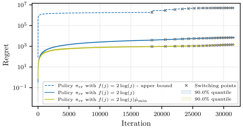
Figure 1: Comparison of the theoretical and simulated regret for $\pi_{\text{cr}}$.

VI-C Simulation Results for Confidence Radius Policy $\pi_{\text{cr}}$

We first study the CMAB policy $\pi_{\text{cr}}$, which has been introduced in Section IV. Note that the confidence radii are not dependent on the actual mean worker response times. In case the workers have small response times, the confidence radii $\theta_{i}\left(j\right)$ might be very dominant compared to the empirical mean estimates $\hat{\mu}_{i}$, leading to a frequent employment of suboptimal workers. For practical purposes, it may thus be beneficial to use an adapted confidence radius with $f(j)=2\log(j)\hat{\mu}_{\min}$, where $\hat{\mu}_{\min}=\min_{i\in\left[1,n\right]}\hat{\mu}_{i}$, that balances the confidence radius and the mean estimate. In Fig. 1, we compare the theoretical regret guarantee in Theorem 2 to practical results for both confidence bound choices. As the theoretical guarantee is a worst case analysis, the true performance is underestimated significantly. We can see that using $f(j)=2\log(j)\hat{\mu}_{\min}$ significantly improves the regret. However, this comes at the cost of delaying the determination of the fastest workers. While with $f(j)=2\log(j)$ the policy correctly determined all $b$ fastest workers in ten simulation runs, with $f(j)=2\log(j)\hat{\mu}_{\min}$ in one out of ten simulations the algorithm commits to a worker with a suboptimality gap of $0.1$. This reflects the trade-off between the competing objectives of best arm identification and regret minimization discussed in [42]. However, since the fastest workers have been determined eventually with an accuracy of $99.5\%$, the proposed adapted confidence bound seems to be a good choice in practice. Although the theoretical bound is rather loose and deviates from the simulations up to some multiplicative factors, it shows the round-based behavior in a worst-case scenario.

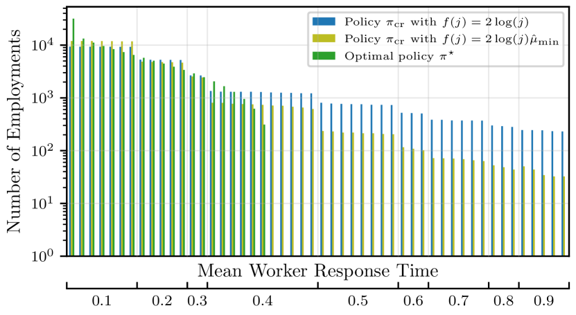
Figure 2: Number of worker employments for $\pi_{\text{cr}}$.

The number of worker employments is shown in Fig. 2, with the workers sorted from fastest to slowest. As expected, compared to the optimal strategy, the LCB-based algorithms have to explore all workers including suboptimal ones. With the adapted confidence bound and compared to $f(j)=2\log(j)$, suboptimal workers are employed significantly less due to the reason above. This also explains the different regrets in Fig. 1.

Figure 3: Comparison of the theoretical and simulated regret for $\pi_{\text{kl}}$.

VI-D Simulation Results for KL-Based Policy $\pi_{\text{kl}}$

The strategy proposed in Section V introduces additional computational overhead for the main node to run a numerical procedure for calculating the LCBs due to the missing analytical closed-form solution. Depending on the computational resources of the main node, this overhead might outweigh the benefits of using the KL-based policy. However, the convergence rate improves significantly compared to the strategy in Section IV. This is reflected by the regret in Fig. 3, where we find the regret bound again as a very pessimistic overestimate. The best workers in this case were determined with an accuracy of $99.0\%$, showing that the impacts of missclassfication can almost be neglected and the regret improves by a factor of approximately ten compared to the results in Section VI-C. The improvement in regret follows directly from the reduced amount of suboptimal worker employments, which is depicted in Fig. 4.

Figure 4: Number of worker employments for $\pi_{\text{kl}}$.

Remark 3.

One could try to find confidence bounds that further minimize the cumulative regret. However, in [42] it was shown that the two goals regret minimization and best arm identification become contradictory at some point. That is, one can either optimize an algorithm towards very confidently determining the best arms out of all available ones, or one could seek to optimize the cumulative regret to the maximum extend. Since in this case we are concerned with both objectives, the goal was to find a policy satisfying them simultaneously.

VI-E Comparison to Adaptive $k$-Sync

In Fig. 5, we analyze the convergence of the algorithms from Section IV (with two different $f(j)$) and Section V, and compare with the optimal policy $\pi^{\star}$ and the adaptive $k$-sync scheme from [8].

Speed. As waiting for the $r$ fastest out of $n>r$ workers is on average faster than waiting for all out of $r$ workers, the adaptive $k$-sync strategy from [8] is significantly faster than our proposed scheme. Comparing $\pi^{\star}$ to the performance of $\pi_{\text{cr}}$ with $f(j)=2\log(j)$, learning the mean worker speeds slows down the convergence by a factor of almost three. This is because the chosen confidence radius mostly dominates the mean response time estimates of the workers, which leads to an emphasis on exploration, i.e., more confident estimates at the expense of sampling slow workers more often. While the confidence bound adapted by $\hat{\mu}_{\min}$ accounts for this drawback, $\pi_{\text{kl}}$ achieves the best results. However, this comes at the expense of more computational load to calculate the LCBs.

Figure 5: Comparison to adaptive $k$-sync [8] with limited budget $B$.

Worker employment. Considering the same cost, our proposed scheme is able to achieve significantly better results. In particular, with a total budget of $B<$1.3\text{\times}{10}^{5}$$ computations, the CMAB-based strategy reaches an error of $\approx$2\text{\times}{10}^{-3}$$ while adaptive $k$-sync achieves an error of only $\approx$6\text{\times}{10}^{1}$$.

Communication. The CMAB schemes had to transfer in total $B<$1.3\text{\times}{10}^{5}$$ models to the workers, while adaptive $k$-sync occupied the transmission link from the main node to the workers $n\cdot T_{b}>$1.5\text{\times}{10}^{6}$$ times. Thus, the downlink communication cost is reduced by more than a factor of ten, whereas the load on the uplink channel from the workers to the main node is $B<$1.3\text{\times}{10}^{5}$$ for both strategies. Consequently, the total amount of channel occupations has been reduced by more than $80\%$, i.e., $2B$ instead of $B+n\cdot T_{b}$.

VII Conclusion

In this paper, we have introduced a cost-efficient distributed machine learning scheme that assigns random tasks to fast workers and leverages all computations. The number of workers employed per iteration increases as the algorithm evolves. To speed up the convergence, we introduced the use of a CMAB model, for which we provided theoretical regret guarantees and simulation results. While our scheme is inferior to the adaptive $k$-sync strategy from [8] in terms of speed, it achieves much lower errors with the same computational efforts while reducing the communication load significantly.

As further research directions, one could derive tighter regret bounds and improve the choice of the confidence bound. In addition, one can consider the setting in which the underlying distributions of the response times of the workers vary over time. Furthermore, relaxing the shared memory assumption and instead fixing the task distribution to the workers opens up an interesting trade-off between the average waiting time per iteration and the convergence rate for distributed machine learning with CMABs. On a high level, this holds because the main node should sample different subsets of the data at every iteration. Hence, the main node cannot always employ the fastest workers.

Appendix A Proof of Proposition 1

Let $F_{\texttt{Z}}$ be the cumulative distribution function of random variable Z, and let $\mathcal{P}\left(\mathcal{I}\right)$ be the power set of $\mathcal{I}$. Consider exponentially distributed random variables indexed by a set $\mathcal{I}$, i.e., $\texttt{Z}_{p}\sim\exp\left(\lambda_{p}\right)$, $p\in\mathcal{I}$, with different rates $\lambda_{p}$ and cumulative distribution function $F_{\texttt{Z}_{p}}(x)=1-e^{-\lambda_{p}x}$. Then, we can derive the maximum order statistics, i.e., the expected value of the largest of their realizations, as

$$\mathbb{E}\left[\max\limits_{p\in\mathcal{I}}\texttt{Z}_{p}\right] =\int\limits_{0}^{\infty}\left(1-F_{\max\limits_{p\in\mathcal{I}}\texttt{Z}_{p}}(x)\right)dx$$

$$=\int\limits_{0}^{\infty}\left(1-\prod\limits_{p\in\mathcal{I}}F_{\texttt{Z}_{p}}(x)\right)dx$$

$$=\int\limits_{0}^{\infty}\left(1-\prod\limits_{p\in\mathcal{I}}(1-e^{-\lambda_{p}x})\right)dx$$

$$=\int\limits_{0}^{\infty}\left(1-\sum\limits_{\mathcal{S}\in\mathcal{P}\left(\mathcal{I}\right)}\left(-1\right)^{|\mathcal{S}|}e^{-\sum\limits_{\xi\in\mathcal{S}}\lambda_{\xi}x}dx\right)$$

$$=\sum\limits_{\mathcal{S}\in\mathcal{P}\left(\mathcal{I}\right)\setminus\emptyset}\left(-1\right)^{|\mathcal{S}|-1}\int\limits_{0}^{\infty}e^{-\sum\limits_{\xi\in\mathcal{S}}\lambda_{\xi}x}dx,$$

Solving the integral concludes the proof.

Appendix B Proof of Theorem 1

To prove the probabilistic bound in Theorem 1, we utilize the well-known Chebychev’s inequality. It provides a handle on the probability that a random variable Z deviates from its mean by more than a given absolute value based on its variance. As given in [43, p. 19], the relation denotes as

$$\Pr\left(\left|\texttt{Z}-\mathbb{E}\left[\texttt{Z}\right]\geq\varepsilon\right|\right)\leq\frac{\textup{Var}\left[\texttt{Z}\right]}{\varepsilon^{2}}.$$ (9)

The probability $1-\Pr(j,r)$ for a certain confidence parameter $\epsilon$ that the upper bound of the time spent in round $r$, i.e., $\mu_{\mathcal{A}^{r,\star}}\!\!\left(\min\left\{j,T_{r}\right\}-T_{r-1}\right)\!\left(1+\epsilon\right)$, is smaller than the true run-time of the algorithm in iteration $j$, where $j>T_{r-1}$, can be calculated by applying Chebychev’s inequality given in (9):

$$1\!-\!\Pr(j,r)=\, \begin{aligned} \Pr\Bigg{(}\sum\limits_{y=T_{r-1}+1}^{\min\left\{j,T_{r}\right\}}\!\!\!\!&Z_{\mathcal{A}^{r,\star}}^{y}\!\!-\!\mu_{\mathcal{A}^{r,\star}}\!\left(\min\left\{j,T_{r}\right\}-T_{r-1}\right)\\ &\geq\epsilon\cdot\mu_{\mathcal{A}^{r,\star}}\left(\min\left\{j,T_{r}\right\}-T_{r-1}\right)\vphantom{\sum\limits_{y=T_{r-1}+1}^{\min\left\{j,T_{r}\right\}}}\Bigg{)}\end{aligned}$$

$$\leq\frac{\textup{Var}\left[\sum\limits_{y=T_{r-1}+1}^{\min\left\{j,T_{r}\right\}}Z_{\mathcal{A}^{r,\star}}^{y}\right]}{\mu_{\mathcal{A}^{r,\star}}^{2}\left(\min\left\{j,T_{r}\right\}-T_{r-1}\right)^{2}\epsilon^{2}}$$

$$\leq\frac{\sigma_{\mathcal{A}^{r,\star}}^{2}}{\mu_{\mathcal{A}^{r,\star}}^{2}\left(\min\left\{j,T_{r}\right\}-T_{r-1}\right)\epsilon^{2}}$$

Then, the probability that $t_{j}$ is underestimated in any of the rounds up to iteration $j$ eventually can be given as

$$1\!-\!\Pr(j)\! =\!1-\!\!\!\!\!\!\!\!\!\!\!\prod\limits_{r\in\left[1,b\right]:j>T_{r-1}}\!\!\left(1-(1-\Pr(j,r))\right)$$

$$\leq 1-\!\!\!\!\!\!\!\!\!\!\!\prod\limits_{r\in\left[1,b\right]:j>T_{r-1}}\!\!\!\!\left(\!1-\frac{\sigma_{\mathcal{A}^{r,\star}}^{2}}{\mu_{\mathcal{A}^{r,\star}}^{2}\left(\min\left\{j,T_{r}\right\}-T_{r-1}\right)\epsilon^{2}}\!\right)\!.$$

Taking the complementary event concludes the proof.

Appendix C Well-Known Tail Bounds

In Appendix D, we utilize well-known properties of tail distributions of sub-gamma and sub-Gaussian random variables, which we provide in the following for completeness.

Sub-gamma tail bound: For $\texttt{Z}\sim\text{Sub}\Gamma\left(\alpha,\beta\right)$ with variance $\sigma^{2}=\frac{\alpha}{\beta^{2}}$ and scale $c=\frac{1}{\beta}$, we have that [43, p. 29] $\Pr\left(\texttt{Z}>\sqrt{2\sigma^{2}\varepsilon}+c\varepsilon\right)\leq\exp\left(-\varepsilon\right).$

Sub-Gaussian tail bound: Resulting from the Cramér-Chernoff method, we obtain for any $\texttt{Z}\sim\text{SubG}\left(\sigma^{2}\right)$ [44, p. 77] that $P\left(\texttt{Z}\leq-\varepsilon\right)\leq\exp\left(-\frac{\varepsilon^{2}}{2\sigma^{2}}\right).$

Appendix D Proof of Theorem 2

While we will benefit from the proof strategies in [27] and [37], our analysis differs in that we consider an unbounded distribution of the rewards, which requires us to investigate the properties of sub-gamma distributions and to use different confidence bounds. Also, compared to [27], we deal with LCBs instead of UCBs since we want to minimize the response time of a superarm, i.e., the time spent per iteration. This problem setting was briefly discussed in [37]. While the authors bound the probability of overestimating an entire suboptimal superarm in [37], we bound the probability of individual suboptimal arm choices. This is justified by independent outcomes across arms and by the combined outcome of a superarm being a monotonically non-decreasing function of the individual arms’ rewards, that is, the workers’ mean response times. A superarm $\mathcal{A}^{r}(j)$ is considered suboptimal if $\mu_{\mathcal{A}^{r}(j)}>\mu_{\mathcal{A}^{r,\star}}$ and a single arm $\mathcal{A}^{r}_{\nu}(j)$ is suboptimal if $\mu_{\mathcal{A}^{r}_{\nu}(j)}>\mu_{\mathcal{A}^{r,\star}_{\nu}}$. In addition to the counter $T_{i}\left(j\right)$, for every arm $i\in[n]$, we introduce the counter $C_{i,e}\left(j\right)\leq T_{i}\left(j\right)$. The integer $e$ refers to the maximum cardinality of all possible superarm choices, i.e., $C_{i,e}\left(j\right)$ is valid for all rounds $r\leq e$. If a suboptimal superarm $\mathcal{A}^{r}(j)$ is chosen, $C_{i,e}\left(j\right)$ is incremented only for the arm $i\in\mathcal{A}^{r}(j)$ that has been pulled the least until this point in time, i.e., $i=\mathcal{A}^{r}_{\nu_{\text{min}}}(j)$, where $\nu_{\text{min}}=\text{arg}\min_{\nu\in\mathcal{A}^{r}(j)}T_{\nu}\!\left(j\right)$. Hence, $\sum_{i=1}^{n}C_{i,e}\left(j\right)$ equals the number of suboptimal superarm pulls. Let $\mathcal{W}^{\leq e}$ be the set of all superarms with a maximum cardinality of $e$, i.e., $\mathcal{W}^{\leq e}\coloneqq\bigcup_{r\leq e}\mathcal{W}^{r}$, and $T_{\mathcal{A}}\!\left(j\right)$ the number of times superarm $\mathcal{A}$ has been pulled until iteration $j$. We have

$$\sum\limits_{\mathcal{U}\in\mathcal{W}^{\leq e}:\mu_{\mathcal{U}}>\mu_{\mathcal{A}^{\left|\mathcal{U}\right|,\star}}}\mathbb{E}\left[T_{\mathcal{U}}\!\left(j\right)\right]=\sum\limits_{i=1}^{n}\mathbb{E}\left[C_{i,e}\left(j\right)\right].$$ (10)

Applying [44, Lemma 4.5] to express the regret in terms of the suboptimality gaps in iteration $j$ of round $r$, i.e., $T_{r-1}<j\leq T_{r}$ and $e=r$, we use (10) and obtain

$$R_{j}^{\pi_{\text{cr}}} =\sum\limits_{\mathcal{U}\in\mathcal{W}^{\leq e}:\mu_{\mathcal{U}}>\mu_{\mathcal{A}^{\left|\mathcal{U}\right|,\star}}}\Delta_{\mathcal{U}}\,\mathbb{E}\left[T_{\mathcal{U}}\!\left(j\right)\right]$$

$$\leq\max\limits_{r\in\left[1,b\right]:j>T_{r-1}}\Delta_{\mathcal{A}^{r},\max}\cdot\sum\limits_{i=1}^{n}\mathbb{E}\left[C_{i,e}\left(j\right)\right].$$ (11)

To conclude the proof of Theorem 2 we need the following intermediate results.

Lemma 4.

Let $\left|\mathcal{A}^{r}(y)\right|\leq e$ hold $\forall y\in\left[j\right]$. For any $h\geq 0$, we can bound the expectation of $C_{i,e}\left(j\right)$, $i\in\left[n\right]$, as

$$\mathbb{E}\left[C_{i,e}\left(j\right)\right]\leq \,h+\sum\limits_{y=1}^{j}j^{2}\cdot\sum\limits_{\nu=1}^{\left|\mathcal{A}^{r}(y)\right|}\Pr\left(\mu_{\mathcal{A}^{r}_{\nu}(y)}>\mu_{\mathcal{A}^{r,\star}_{\nu}},\right.$$

$$\left.\text{LCB}_{\mathcal{A}^{r}_{\nu}(y)}(y)\leq\text{LCB}_{\mathcal{A}^{r,\star}_{\nu}}(y)\right).$$

By construction, for a superarm $\mathcal{A}^{r}(j)$ with $\left|\mathcal{A}^{r}(j)\right|\leq e$ it holds for all $\nu\in[1,\left|\mathcal{A}^{r}(j)\right|]$ and $i\in\mathcal{A}^{r}(j)$ that $T_{\mathcal{A}^{r}_{\nu}(j)}\!\left(j\right)\geq C_{i,e}\left(j\right)$. By applying Lemma 4 with $h\geq 0$, we thus have $T_{\mathcal{A}^{r}_{\nu}(j)}\!\left(j\right)\geq C_{i,e}\left(j\right)\geq h$. To bound the probability of choosing a suboptimal arm over which we sum in Lemma 4, we use Lemma 5.

Lemma 5.

The probability of the $\nu$-th fastest arm of $\mathcal{A}^{r}(j)$ being suboptimal given that $T_{\mathcal{A}^{r}_{\nu}(j)}\!\left(j\right)\geq\lceil\frac{48\log(j)}{\min\{\delta_{\min}^{2},\delta_{\min}\}}\rceil$, is bounded from above as

$$\Pr\left(\mu_{\mathcal{A}^{r}_{\nu}(j)}>\mu_{\mathcal{A}^{r,\star}_{\nu}},\text{LCB}_{\mathcal{A}^{r}_{\nu}(j)}(j)\leq\text{LCB}_{\mathcal{A}^{r,\star}_{\nu}}(j)\right)$$

$$\leq j^{-4\min\left\{\lambda_{\min},\lambda_{\min}^{2}\right\}}+j^{-4\lambda_{\min}}.$$ (12)

Having the results of Lemma 4 and Lemma 5, and choosing $h=\lceil\frac{48\log(j)}{\min\{\delta_{\min}^{2},\delta_{\min}\}}\rceil$, for $\lambda_{\min}\geq 1$ we have

$$\mathbb{E}\left[C_{i,e}\left(j\right)\right] \leq h+\sum\limits_{y=1}^{j}j^{2}\cdot\sum\limits_{\nu=1}^{\left|\mathcal{A}^{r}(y)\right|}\Pr\left(\mu_{\mathcal{A}^{r}_{\nu}(y)}>\mu_{\mathcal{A}^{r,\star}_{\nu}},\right.$$

$$\left.\text{LCB}_{\mathcal{A}^{r}_{\nu}(y)}(y)\leq\text{LCB}_{\mathcal{A}^{r,\star}_{\nu}}(y)\right)$$

$$\leq\left\lceil\frac{48\log(j)}{\min\{\delta_{\min}^{2},\delta_{\min}\}}\right\rceil+\sum\limits_{y=1}^{j}j^{2}\cdot\sum\limits_{\nu=1}^{e}2j^{-4\lambda_{\min}}$$

$$\leq\frac{48\log(\min\left\{j,T_{r}\right\})}{\min\left\{\delta_{\min}^{2},\delta_{\min}\right\}}+1+e\cdot\frac{\pi}{3},$$ (13)

where the last step relates to the Basel problem of a $p$-series. Plugging the bound in (13) into (11) concludes the proof.

The proof of Lemma 4 uses standard techniques from the literature on MABs and is given in the following for completeness. The proof of Lemma 5 is given afterwards.

Proof of Lemma 4.

At first, we bound the counter $C_{i,e}\left(j\right)$ from below by introducing an arbitrary parameter $h$ that eventually serves to limit the probability of choosing a suboptimal arm. Similar to [37], we have

$$C_{i,e}(j)\leq\begin{aligned} &h+\sum\limits_{y=1}^{j}\mathds{1}\left\{\exists\;1\leq\nu\leq\left|\mathcal{A}^{r}(y)\right|:\right.\left.\mu_{\mathcal{A}^{r}_{\nu}(y)}>\mu_{\mathcal{A}^{r,\star}_{\nu}},\right.\\ &\left.\text{LCB}_{\mathcal{A}^{r}_{\nu}(y)}(y)\right.\left.\leq\text{LCB}_{\mathcal{A}^{r,\star}_{\nu}}(y)\right\}\end{aligned}$$

$$\,\,\,\,\leq\begin{aligned} &h+\sum\limits_{y=1}^{j}\sum\limits_{\nu=1}^{\left|\mathcal{A}^{r}(y)\right|}\mathds{1}\{\mu_{\mathcal{A}^{r}_{\nu}(y)}>\mu_{\mathcal{A}^{r,\star}_{\nu}},\\ &\text{LCB}_{\mathcal{A}^{r}_{\nu}(y)}(y)\leq\text{LCB}_{\mathcal{A}^{r,\star}_{\nu}}(y)\}\end{aligned}$$

$$\,\,\,\,\leq\begin{aligned} &h+\sum\limits_{y=1}^{j}\sum\limits_{\nu=1}^{\left|\mathcal{A}^{r}(y)\right|}\mathds{1}\{\mu_{\mathcal{A}^{r}_{\nu}(y)}>\mu_{\mathcal{A}^{r,\star}_{\nu}},\\ &\min\limits_{h\leq T_{\mathcal{A}^{r}_{\nu}(y)}\!\left(y\right)\leq j}\text{LCB}_{\mathcal{A}^{r}_{\nu}(y)}(y)\leq\max\limits_{1\leq T_{\mathcal{A}^{r,\star}_{\nu}}\!\left(y\right)\leq j}\text{LCB}_{\mathcal{A}^{r,\star}_{\nu}}(y)\}\end{aligned}$$

$$\,\,\,\,\leq\begin{aligned} &h+\sum\limits_{y=1}^{j}\sum\limits_{T_{\mathcal{A}^{r}_{\nu}(y)}\!\left(y\right)=h}^{j}\sum\limits_{T_{\mathcal{A}^{r,\star}_{\nu}}\!\left(y\right)=1}^{j}\sum\limits_{\nu=1}^{\left|\mathcal{A}^{r}(y)\right|}\mathds{1}\{\mu_{\mathcal{A}^{r}_{\nu}(y)}>\mu_{\mathcal{A}^{r,\star}_{\nu}},\\ &\text{LCB}_{\mathcal{A}^{r}_{\nu}(y)}(y)\leq\text{LCB}_{\mathcal{A}^{r,\star}_{\nu}}(y)\}\end{aligned}$$

$$\,\,\,\,\leq\begin{aligned} &h+\sum\limits_{y=1}^{j}j^{2}\sum\limits_{\nu=1}^{\left|\mathcal{A}^{r}(y)\right|}\mathds{1}\{\mu_{\mathcal{A}^{r}_{\nu}(y)}>\mu_{\mathcal{A}^{r,\star}_{\nu}},\\ &\text{LCB}_{\mathcal{A}^{r}_{\nu}(y)}(y)\leq\text{LCB}_{\mathcal{A}^{r,\star}_{\nu}}(y)\},\end{aligned}$$

where the first line describes the event of choosing a suboptimal superarm in terms of the events that the LCB of any suboptimal $\nu$-fastest arm in $\mathcal{A}^{r}(j)$ is less than or equal to the LCB of the $\nu$-fastest arm in $\mathcal{A}^{r,\star}$. To conclude the proof, we take the expectation on both sides. ∎

Proof of Lemma 5.

As given in [27], to overestimate the $\nu$-th fastest arm of $\mathcal{A}^{r}(j)$, i.e., for $\text{LCB}_{\mathcal{A}^{r}_{\nu}(j)}(j)\leq\text{LCB}_{\mathcal{A}^{r,\star}_{\nu}}(j)$ to hold, at least one of the following events must be satisfied:

$$\mu_{\mathcal{A}^{r,\star}_{\nu}} >\mu_{\mathcal{A}^{r}_{\nu}(j)}-2\theta_{\mathcal{A}^{r}_{\nu}(j)}\left(j\right),$$ (14)

$$\hat{\mu}_{\mathcal{A}^{r,\star}_{\nu}}(j) \geq\mu_{\mathcal{A}^{r,\star}_{\nu}}+\theta_{\mathcal{A}^{r,\star}_{\nu}}\left(j\right),$$ (15)

$$\hat{\mu}_{\mathcal{A}^{r}_{\nu}(j)}(j) \leq\mu_{\mathcal{A}^{r}_{\nu}(j)}-\theta_{\mathcal{A}^{r}_{\nu}(j)}\left(j\right).$$ (16)

Let in the following $f(j)\coloneqq 2\log(j)$. We first show that the requirement $T_{\mathcal{A}^{r}_{\nu}(j)}\!\left(j\right)\geq\lceil\frac{24f(j)}{\min\{\delta_{\min}^{2},\delta_{\min}\}}\rceil\coloneqq\ell$ guarantees that $\mu_{\mathcal{A}^{r,\star}_{\nu}}-\mu_{\mathcal{A}^{r}_{\nu}(j)}+2\theta_{\mathcal{A}^{r}_{\nu}(j)}\left(j\right)\leq 0$, for all $\mathcal{A}^{r}(j)\in\mathcal{W}^{r}$ with $r\in[1,b]$, $\nu\in[1,r]$ and $\mu_{\mathcal{A}^{r}_{\nu}(j)}>\mu_{\mathcal{A}^{r,\star}_{\nu}}$, thus making the event (14) a zero-probability event. We have

$$\mu_{\mathcal{A}^{r,\star}_{\nu}} -\mu_{\mathcal{A}^{r}_{\nu}(j)}+2\left(\sqrt{\frac{4f(j)}{T_{\mathcal{A}^{r}_{\nu}(j)}\!\left(j\right)}}+\frac{2f(j)}{T_{\mathcal{A}^{r}_{\nu}(j)}\!\left(j\right)}\right)$$

$$\leq\mu_{\mathcal{A}^{r,\star}_{\nu}}-\mu_{\mathcal{A}^{r}_{\nu}(j)}+2\left(\sqrt{\frac{4f(j)}{h}}+\frac{2f(j)}{h}\right)$$

$$\leq-\delta_{\mathcal{A}^{r}_{\nu}(j)}+\delta_{\min}\leq 0.$$

Lemma 6.

Given i.i.d. random variables $Z_{i}^{j}\sim\exp(\lambda_{i})$, $j=1,\dots,T$, the deviation of the empirical mean from the true mean $\hat{\mu}_{i}-\mu_{i}\coloneqq\frac{1}{T}\sum_{j=1}^{T}\left(Z_{i}^{j}-\mathbb{E}[Z_{i}^{j}]\right)$ follows a sub-gamma distribution $\text{Sub}\Gamma\left(T,T\lambda_{i}\right)$ on the right tail and a sub-Gaussian distribution $\text{SubG}\left(\frac{1}{T\lambda_{i}^{2}}\right)$ on the left tail.

We apply Lemma 6 (which is proven below) to bound the probability of the event (15). However, two cases have to be distinguished. For $\lambda_{\min}\geq 1$, we have

$$\Pr\left(\hat{\mu}_{\mathcal{A}^{r,\star}_{\nu}}(j)\geq\mu_{\mathcal{A}^{r,\star}_{\nu}}+\theta_{\mathcal{A}^{r,\star}_{\nu}}\left(j\right)\right)$$

$$=\Pr\left(\hat{\mu}_{\mathcal{A}^{r,\star}_{\nu}}(j)\geq\mu_{\mathcal{A}^{r,\star}_{\nu}}+\sqrt{\frac{4f(j)}{T_{\mathcal{A}^{r,\star}_{\nu}}\!\left(j\right)}}+\frac{2f(j)}{T_{\mathcal{A}^{r,\star}_{\nu}}\!\left(j\right)}\right)$$

$$\leq\Pr\left(\hat{\mu}_{\mathcal{A}^{r,\star}_{\nu}}(j)\geq\mu_{\mathcal{A}^{r,\star}_{\nu}}+\sqrt{\frac{4f(j)}{T_{\mathcal{A}^{r,\star}_{\nu}}\!\left(j\right)\lambda_{\min}}}+\frac{2f(j)}{T_{\mathcal{A}^{r,\star}_{\nu}}\!\left(j\right)}\right)$$

$$\leq\Pr\left(\hat{\mu}_{\mathcal{A}^{r,\star}_{\nu}}(j)\geq\mu_{\mathcal{A}^{r,\star}_{\nu}}\!+\!\sqrt{\frac{4f(j)\lambda_{\min}}{T_{\mathcal{A}^{r,\star}_{\nu}}\!\left(j\right)\!\lambda_{\min}^{2}}}\!+\!\frac{2f(j)\lambda_{\min}}{T_{\mathcal{A}^{r,\star}_{\nu}}\!\left(j\right)\!\lambda_{\min}}\right)$$

$$=\Pr\left(\hat{\mu}_{\mathcal{A}^{r,\star}_{\nu}}(j)\geq\mu_{\mathcal{A}^{r,\star}_{\nu}}\!+\!\sqrt{\frac{8\log(j)\lambda_{\min}^{2}}{T_{\mathcal{A}^{r,\star}_{\nu}}\!\left(j\right)\lambda_{\min}^{2}}}+\frac{4\log(j)\lambda_{\min}^{2}}{T_{\mathcal{A}^{r,\star}_{\nu}}\!\left(j\right)\lambda_{\min}}\right)$$

$$\leq\exp{-4\log(j)\lambda_{\min}}\leq j^{-4\lambda_{\min}},$$

where in the penultimate step we used the sub-gamma tail bound given in Appendix C with $\varepsilon=2\log(j)\lambda_{\min}$.

In contrast, if $\lambda_{\min}<1$

$$\Pr\left(\hat{\mu}_{\mathcal{A}^{r,\star}_{\nu}}(j)\geq\mu_{\mathcal{A}^{r,\star}_{\nu}}+\theta_{\mathcal{A}^{r,\star}_{\nu}}\left(j\right)\right)$$

$$=\Pr\left(\hat{\mu}_{\mathcal{A}^{r,\star}_{\nu}}(j)\geq\mu_{\mathcal{A}^{r,\star}_{\nu}}+\sqrt{\frac{4f(j)}{T_{\mathcal{A}^{r,\star}_{\nu}}\!\left(j\right)}}+\frac{2f(j)}{T_{\mathcal{A}^{r,\star}_{\nu}}\!\left(j\right)}\right)$$

$$\leq\Pr\left(\hat{\mu}_{\mathcal{A}^{r,\star}_{\nu}}(j)\geq\mu_{\mathcal{A}^{r,\star}_{\nu}}+\sqrt{\frac{4f(j)}{T_{\mathcal{A}^{r,\star}_{\nu}}\!\left(j\right)}}+\frac{2f(j)\lambda_{\min}}{T_{\mathcal{A}^{r,\star}_{\nu}}\!\left(j\right)}\right)$$

$$=\Pr\left(\hat{\mu}_{\mathcal{A}^{r,\star}_{\nu}}(j)\geq\mu_{\mathcal{A}^{r,\star}_{\nu}}+\sqrt{\frac{4f(j)\lambda_{\min}^{2}}{T_{\mathcal{A}^{r,\star}_{\nu}}\!\left(j\right)\lambda_{\min}^{2}}}+\frac{2f(j)\lambda_{\min}^{2}}{T_{\mathcal{A}^{r,\star}_{\nu}}\!\left(j\right)\lambda_{\min}}\right)$$

$$=\Pr\left(\hat{\mu}_{\mathcal{A}^{r,\star}_{\nu}}(j)\geq\mu_{\mathcal{A}^{r,\star}_{\nu}}+\sqrt{\frac{8\log(j)\lambda_{\min}^{2}}{T_{\mathcal{A}^{r,\star}_{\nu}}\!\left(j\right)\lambda_{\min}^{2}}}+\frac{4\log(j)\lambda_{\min}^{2}}{T_{\mathcal{A}^{r,\star}_{\nu}}\!\left(j\right)\lambda_{\min}}\right)$$

$$\leq\exp{-4\log(j)\lambda_{\min}^{2}}$$

$$\leq j^{-4\lambda_{\min}^{2}},$$

where in the penultimate line we used the sub-gamma tail bound in Appendix C with $\varepsilon=2\log(j)\lambda_{\min}^{2}$.

For the event in (16), we have

$$\Pr\left(\hat{\mu}_{\mathcal{A}^{r}_{\nu}(j)}(j)\leq\mu_{\mathcal{A}^{r}_{\nu}(j)}-\theta_{\mathcal{A}^{r}_{\nu}(j)}\left(j\right)\right)$$

$$=\Pr\left(\hat{\mu}_{\mathcal{A}^{r}_{\nu}(j)}(j)\leq\mu_{\mathcal{A}^{r}_{\nu}(j)}-\sqrt{\frac{4f(j)}{T_{\mathcal{A}^{r}_{\nu}(j)}\!\left(j\right)}}-\frac{2f(j)}{T_{\mathcal{A}^{r}_{\nu}(j)}\!\left(j\right)}\right)$$

$$\leq\Pr\left(\hat{\mu}_{\mathcal{A}^{r}_{\nu}(j)}(j)\leq\mu_{\mathcal{A}^{r}_{\nu}(j)}-\sqrt{\frac{4f(j)}{T_{\mathcal{A}^{r}_{\nu}(j)}\!\left(j\right)}}\right)$$

$$\leq\exp{-4\lambda_{\mathcal{A}^{r}_{\nu}(j)}^{2}\log(j)}$$

$$\leq j^{-4\lambda_{\mathcal{A}^{r}_{\nu}(j)}^{2}}\leq j^{-4\lambda_{\min}^{2}}\leq j^{-4\lambda_{\min}},$$

where we used the sub-Gaussian tail bound given in Appendix C. ∎

Proof of Lemma 6.

To conduct the proof, we express the independently and identically distributed random variables $Z_{i}^{j}\sim\exp(\lambda_{i})$, $j\in[1,T]$ in terms of its moment generating functions $M_{\texttt{Z}_{i}}(\phi)=\mathbb{E}\left[e^{\phi\texttt{Z}_{i}}\right]=\frac{\lambda_{i}}{\lambda_{i}-\phi}$, which is defined for $\phi<\lambda$. Summing the identically distributed realizations is equivalent to multiplying its moment generating functions, i.e., $\sum_{j=1}^{T}Z_{i}^{j}\leftrightarrow\prod_{j=1}^{T}M_{Z_{i}^{j}}(\phi)=\left(\frac{\lambda_{i}}{\lambda_{i}-\phi}\right)^{T}$, which describes a random variable related to a gamma distribution with shape $T$ and rate $\lambda_{i}$. The empirical mean $\hat{\mu}_{i}=\frac{1}{T}\sum_{j=1}^{T}Z_{i}^{j}$ is thus distributed according to the scaled gamma distribution $\Gamma(T,\lambda_{i}T)$ with mean $\mu_{i}=\frac{1}{\lambda_{i}}$ and variance $\sigma^{2}=\frac{1}{T\lambda_{i}^{2}}$. Thus, $\hat{\mu}_{i}-\mu_{i}$ is a centered gamma distributed random variable, which according to [43, pp. 27] has the properties stated in Lemma 6. ∎

Appendix E Proof of Theorem 3

In the following, we prove the regret bounds given in Theorem 3 based on the analysis in [28]. In particular, we adapt the regret proof in [28] for single arm choices to prove a combinatorial regret bound. To start with, we use the same counter definitions as in Appendix D and follow the same steps, i.e., we apply [44, Lemma 4.5] and use the interdependencies between the counters, to finally result in (17). Let $e=\max\limits_{r\in\left[1,b\right]:j>T_{r-1}}r$, then

$$R_{j}^{\pi} \leq\max\limits_{r\in\left[1,b\right]:j>T_{r-1}}\Delta_{\mathcal{A}^{r},\max}\cdot\sum\limits_{i=1}^{n}\mathbb{E}\left[C_{i,e}\left(j\right)\right].$$ (17)

To conclude, we need to bound the expectation of $C_{i,e}\left(j\right)$. A handle on this is given in the following Lemma 7.

Lemma 7.

The expectation of the suboptimal arm counter $C_{i,e}\left(j\right)$ for superarms $\mathcal{A}^{r}(y)$, $y\in\left[j\right]$, with maximum cardinality $e$, i.e., $\forall y\in\left[1,j\right]$, $\left|\mathcal{A}^{r}(r)\right|\leq e$, LCBs according to (7), and $f(j)=\log(j)+3\log\left(\log\left(j\right)\right)$, $j>3$, can be bounded as

$$\mathbb{E}\left[C_{i,e}\left(j\right)\right] \leq e\left(7\log(\log(j))+\frac{1+\epsilon}{\text{D}_{\text{KL},\min}}f(j)+Q_{j}(\epsilon)\right),$$

where $Q_{j}(\epsilon)=\frac{\exp\left(-\text{D}_{\text{KL}\epsilon,\min}\left(\frac{1+\epsilon}{\text{D}_{\text{KL},\max}}f(j)-1\right)\right)}{1-\exp(-\text{D}_{\text{KL}\epsilon,\min})}$.

Plugging the result of Lemma 7 into (17) concludes the proof of Theorem 3. It remains to prove Lemma 7.

Proof of Lemma 7.

To prove Lemma 7, we need a result from [28], which we state in our notation and for our problem in Lemma 8. We briefly explain why this result holds in our setting.

Lemma 8 (​​[28]).

The probability of overestimating the $\nu$-th fastest element of $\mathcal{A}^{r}(j)$ in any of the iterations up to iteration $j$ given that the element is suboptimal, a decision process $\pi_{\text{kl}}$ based on the LCB in (7) and $K_{j}=\Big{\lfloor}\frac{1+\epsilon}{\text{D}_{\text{KL}}^{-}\left(\mu_{\mathcal{A}^{r}_{\nu}(j)}\|\mu_{\mathcal{A}^{r,\star}_{\nu}}\right)}f(j)\Big{\rfloor}$ can be upper bounded as

$$\sum\limits_{y=1}^{j} \Pr\left(\mu_{\mathcal{A}^{r}_{\nu}(y)}>\mu_{\mathcal{A}^{r,\star}_{\nu}},\text{LCB}_{\mathcal{A}^{r}_{\nu}(y)}(y)\leq\text{LCB}_{\mathcal{A}^{r,\star}_{\nu}}(y)\right)$$

$$\leq 7\log(\log(j))+\frac{1+\epsilon}{\text{D}_{\text{KL}}^{-}\left(\mu_{\mathcal{A}^{r}_{\nu}(j)}\|\mu_{\mathcal{A}^{r,\star}_{\nu}}\right)}f(j)$$

$$+\frac{\exp\left(-\text{D}_{\text{KL}}\left(\phi(\epsilon,\mu_{\mathcal{A}^{r,\star}_{\nu}},\mu_{\mathcal{U}_{\nu}})\|\mu_{\mathcal{A}^{r}_{\nu}(j)}\right)K_{j}\right)}{1-\exp(-\text{D}_{\text{KL}}\left(\phi(\epsilon,\mu_{\mathcal{A}^{r,\star}_{\nu}},\mu_{\mathcal{U}_{\nu}})\|\mu_{\mathcal{A}^{r}_{\nu}(j)}\right)},$$

where $\phi(\epsilon,\mu_{\mathcal{A}^{r,\star}_{\nu}},\mu_{\mathcal{A}^{r}_{\nu}(j)})$ defined on the open interval $]\mu_{\mathcal{A}^{r,\star}_{\nu}},\mu_{\mathcal{A}^{r}_{\nu}(j)}[$ is calculated such that $\text{D}_{\text{KL}}\left(\phi(\epsilon,\mu_{\mathcal{A}^{r,\star}_{\nu}},\mu_{\mathcal{A}^{r}_{\nu}(j)})\|\mu_{\mathcal{A}^{r,\star}_{\nu}}\right)=\text{D}_{\text{KL}}\left(\mu_{\mathcal{A}^{r}_{\nu}(j)}\|\mu_{\mathcal{A}^{r,\star}_{\nu}}\right)/(1+\epsilon)$.

Sketch of proof.

The authors of [28] bound the probability of choosing a suboptimal arm based on a KL-divergence-based UCB for all distributions being part of the exponential family. As we can mirror the probability density function of the exponential distribution at the y-axis and result with a distribution from of the exponential family, we can transfer our LCB setting to an equivalent UCB setting. Thus, by symmetry, the performance guarantees of the non-combinatorial KL-based policy for the exponential family apply. ∎

Starting with a similar approach as in the proof of Lemma 4 and by help of the relation given in Lemma 8, we can bound the expectation of the counter $C_{i,e}\left(j\right)$ as

$$\mathbb{E}\left[C_{i,e}\left(j\right)\right]\leq\sum\limits_{y=1}^{j}\Pr(\exists\;1\leq\nu\leq\left|\mathcal{A}^{r}(y)\right|:\mu_{\mathcal{A}^{r}_{\nu}(y)}>\mu_{\mathcal{A}^{r,\star}_{\nu}},$$

$$\text{LCB}_{\mathcal{A}^{r}_{\nu}(y)}(y)\leq\text{LCB}_{\mathcal{A}^{r,\star}_{\nu}}(y))\!$$

$$\leq\sum\limits_{y=1}^{j}\sum\limits_{\nu=1}^{\left|\mathcal{A}^{r}(y)\right|}\Pr\left(\text{LCB}_{\mathcal{A}^{r}_{\nu}(y)}(y)\leq\text{LCB}_{\mathcal{A}^{r,\star}_{\nu}}(y),\mu_{\mathcal{A}^{r}_{\nu}(y)}>\mu_{\mathcal{A}^{r,\star}_{\nu}}\right)$$ (18)

$$\leq\sum\limits_{\nu=1}^{e}\sum\limits_{y=1}^{j}\Pr\left(\text{LCB}_{\mathcal{A}^{r}_{\nu}(y)}(y)\leq\text{LCB}_{\mathcal{A}^{r,\star}_{\nu}}(y),\mu_{\mathcal{A}^{r}_{\nu}(y)}>\mu_{\mathcal{A}^{r,\star}_{\nu}}\right)$$ (19)

$$\leq\sum\limits_{\nu=1}^{e}7\log(\log(j))+\frac{1+\epsilon}{\text{D}_{\text{KL}}^{-}\left(\mu_{\mathcal{A}^{r}_{\nu}(j)}\|\mu_{\mathcal{A}^{r,\star}_{\nu}}\right)}f(j)$$

$$+\frac{\exp\left(-\text{D}_{\text{KL}}\left(\phi(\epsilon,\mu_{\mathcal{A}^{r,\star}_{\nu}},\mu_{\mathcal{U}_{\nu}})\|\mu_{\mathcal{A}^{r}_{\nu}(j)}\right)K_{j}\right)}{1-\exp(-\text{D}_{\text{KL}}\left(\phi(\epsilon,\mu_{\mathcal{A}^{r,\star}_{\nu}},\mu_{\mathcal{U}_{\nu}})\|\mu_{\mathcal{A}^{r}_{\nu}(j)}\right)}$$

$$\leq e\left(7\log(\log(j))+\frac{1+\epsilon}{\text{D}_{\text{KL},\min}}f(j)+Q_{j}(\epsilon)\right),$$

where from (18) to (19) we used the convention that $\mathds{1}\{\text{LCB}_{\mathcal{A}^{r}_{\nu}(y)}(y)\leq\text{LCB}_{\mathcal{A}^{r,\star}_{\nu}}(y),\\ \mu_{\mathcal{A}^{r}_{\nu}(y)}>\mu_{\mathcal{A}^{r,\star}_{\nu}}\}=0$ if $\nu>\left|\mathcal{A}^{r}(y)\right|$. This concludes the proof. ∎

References

• [1] J. Dean and L. A. Barroso, “The tail at scale,” Communications of the ACM, vol. 56, pp. 74–80, 2013.
• [2] J. Chen, X. Pan, R. Monga, S. Bengio, and R. Jozefowicz, “Revisiting distributed synchronous SGD,” 2017, arXiv preprint arXiv:1604.00981.
• [3] K. Lee, M. Lam, R. Pedarsani, D. Papailiopoulos, and K. Ramchandran, “Speeding up distributed machine learning using codes,” in IEEE International Symposium on Information Theory (ISIT), 2016, pp. 1143–1147.
• [4] R. Tandon, Q. Lei, A. G. Dimakis, and N. Karampatziakis, “Gradient coding: Avoiding stragglers in distributed learning,” in Proc. International Conference on Machine Learning, vol. 70, Aug 2017, pp. 3368–3376.
• [5] H. Robbins and S. Monro, “A stochastic approximation method,” The Annals of Mathematical Statistics, vol. 22, no. 3, pp. 400–407, 1951.
• [6] A. Cotter, O. Shamir, N. Srebro, and K. Sridharan, “Better mini-batch algorithms via accelerated gradient methods,” in Advances in Neural Information Processing Systems, vol. 24, 2011.
• [7] S. Dutta, G. Joshi, S. Ghosh, P. Dube, and P. Nagpurkar, “Slow and stale gradients can win the race: Error-runtime trade-offs in distributed SGD,” in Proc. International Conference on Artificial Intelligence and Statistics, vol. 84, Apr 2018, pp. 803–812.
• [8] S. K. Hanna, R. Bitar, P. Parag, V. Dasari, and S. El Rouayheb, “Adaptive distributed stochastic gradient descent for minimizing delay in the presence of stragglers,” in IEEE International Conference on Acoustics, Speech and Signal Processing (ICASSP), 2020, pp. 4262–4266.
• [9] W. R. Thompson, “On the likelihood that one unknown probability exceeds another in view of the evidence of two samples,” Biometrika, vol. 25, no. 3/4, pp. 285–294, 1933.
• [10] V. Anantharam, P. Varaiya, and J. Walrand, “Asymptotically efficient allocation rules for the multiarmed bandit problem with multiple plays-part i: I.i.d. rewards,” IEEE Transactions on Automatic Control, vol. 32, no. 11, pp. 968–976, 1987.
• [11] G. Liang and U. C. Kozat, “TOFEC: Achieving optimal throughput-delay trade-off of cloud storage using erasure codes,” in IEEE Conference on Computer Communications, 2014, pp. 826–834.
• [12] M. Ye and E. Abbe, “Communication-computation efficient gradient coding,” in International Conference on Machine Learning, 2018, pp. 5610–5619.
• [13] N. Raviv, I. Tamo, R. Tandon, and A. G. Dimakis, “Gradient coding from cyclic MDS codes and expander graphs,” IEEE Transactions on Information Theory, vol. 66, no. 12, pp. 7475–7489, 2020.
• [14] E. Ozfatura, S. Ulukus, and D. Gündüz, “Straggler-aware distributed learning: Communication–computation latency trade-off,” Entropy, vol. 22, no. 5, 2020.
• [15] M. M. Amiri and D. Gündüz, “Computation scheduling for distributed machine learning with straggling workers,” IEEE Transactions on Signal Processing, vol. 67, no. 24, p. 6270–6284, Dec 2019.
• [16] S. Li, S. M. Mousavi Kalan, A. S. Avestimehr, and M. Soltanolkotabi, “Near-optimal straggler mitigation for distributed gradient methods,” in IEEE International Parallel and Distributed Processing Symposium Workshops (IPDPSW), 2018, pp. 857–866.
• [17] R. Bitar, M. Wootters, and S. el Rouayheb, “Stochastic gradient coding for straggler mitigation in distributed learning,” IEEE Journal on Selected Areas in Information Theory, vol. 1, pp. 277–291, 2020.
• [18] R. K. Maity, A. Singh Rawat, and A. Mazumdar, “Robust gradient descent via moment encoding and LDPC codes,” in IEEE International Symposium on Information Theory (ISIT), 2019, pp. 2734–2738.
• [19] Z. Charles, D. Papailiopoulos, and J. Ellenberg, “Approximate gradient coding via sparse random graphs,” 2017, arXiv preprint arXiv:1711.06771.
• [20] S. Wang, J. Liu, and N. Shroff, “Fundamental limits of approximate gradient coding,” Proc. ACM on Measurement and Analysis of Computing Systems, vol. 3, no. 3, Dec 2019.
• [21] H. Wang, Z. Charles, and D. Papailiopoulos, “ErasureHead: Distributed gradient descent without delays using approximate gradient coding,” 2019, arXiv preprint arXiv:1901.09671.
• [22] S. Horii, T. Yoshida, M. Kobayashi, and T. Matsushima, “Distributed stochastic gradient descent using LDGM codes,” in IEEE International Symposium on Information Theory (ISIT), 2019, pp. 1417–1421.
• [23] E. Ozfatura, S. Ulukus, and D. Gündüz, “Distributed gradient descent with coded partial gradient computations,” in IEEE International Conference on Acoustics, Speech and Signal Processing (ICASSP), 2019, pp. 3492–3496.
• [24] ——, “Coded distributed computing with partial recovery,” IEEE Transactions on Information Theory, vol. 68, no. 3, pp. 1945–1959, 2022.
• [25] T. Lai and H. Robbins, “Asymptotically efficient adaptive allocation rules,” Advances in Applied Mathematics, vol. 6, no. 1, pp. 4–22, 1985.
• [26] R. Agrawal, “Sample mean based index policies with o(log n) regret for the multi-armed bandit problem,” Advances in Applied Probability, vol. 27, no. 4, pp. 1054–1078, 1995.
• [27] P. Auer, N. Cesa-Bianchi, and P. Fischer, “Finite-time analysis of the multiarmed bandit problem,” Machine Learning, vol. 47, pp. 235–256, May 2002.
• [28] A. Garivier and O. Cappé, “The KL-UCB algorithm for bounded stochastic bandits and beyond,” in Proc. Conference on Learning Theory, vol. 19, Jun 2011, pp. 359–376.
• [29] O. Cappé, A. Garivier, O.-A. Maillard, R. Munos, and G. Stoltz, “Kullback-leibler upper confidence bounds for optimal sequential allocation,” The Annals of Statistics, vol. 41, no. 3, pp. 1516–1541, 2013.
• [30] W. Jouini and C. Moy, “UCB algorithm for exponential distributions,” 2012, arXiv preprint arXiv:1204.1624.
• [31] S. Bubeck, N. Cesa-Bianchi, and G. Lugosi, “Bandits with heavy tail,” IEEE Transactions on Information Theory, vol. 59, no. 11, pp. 7711–7717, 2013.
• [32] W. Chen, Y. Wang, Y. Yuan, and Q. Wang, “Combinatorial multi-armed bandit and its extension to probabilistically triggered arms,” The Journal of Machine Learning Research, vol. 17, no. 1, pp. 1746–1778, 2016.
• [33] B. Kveton, Z. Wen, A. Ashkan, and C. Szepesvari, “Tight Regret Bounds for Stochastic Combinatorial Semi-Bandits,” in Proc. International Conference on Artificial Intelligence and Statistics, vol. 38, May 2015, pp. 535–543.
• [34] W. Chen, Y. Wang, and Y. Yuan, “Combinatorial multi-armed bandit: General framework and applications,” in Proc. International Conference on Machine Learning, vol. 28, no. 1, Jun 2013, pp. 151–159.
• [35] W. Chen, W. Hu, F. Li, J. Li, Y. Liu, and P. Lu, “Combinatorial multi-armed bandit with general reward functions,” in Advances in Neural Information Processing Systems, vol. 29, 2016, pp. 1651–1659.
• [36] Y. Gai, B. Krishnamachari, and R. Jain, “Learning multiuser channel allocations in cognitive radio networks: A combinatorial multi-armed bandit formulation,” in IEEE Symposium on New Frontiers in Dynamic Spectrum (DySPAN), 2010, pp. 1–9.
• [37] ——, “Combinatorial network optimization with unknown variables: Multi-armed bandits with linear rewards and individual observations,” IEEE/ACM Transactions on Networking, vol. 20, no. 5, pp. 1466–1478, 2012.
• [38] L. Bottou, F. E. Curtis, and J. Nocedal, “Optimization methods for large-scale machine learning,” SIAM Review, vol. 60, no. 2, pp. 223–311, 2018.
• [39] G. C. Pflug, “Non-asymptotic confidence bounds for stochastic approximation algorithms with constant step size,” Monatshefte für Mathematik, vol. 110, no. 3, pp. 297–314, 1990.
• [40] J. Chee and P. Toulis, “Convergence diagnostics for stochastic gradient descent with constant learning rate,” in Proc. International Conference on Artificial Intelligence and Statistics, vol. 84, Apr 2018, pp. 1476–1485.
• [41] S. Pesme, A. Dieuleveut, and N. Flammarion, “On convergence-diagnostic based step sizes for stochastic gradient descent,” in Proc. International Conference on Machine Learning, vol. 119, Jul 2020, pp. 7641–7651.
• [42] Z. Zhong, W. C. Cheung, and V. Y. F. Tan, “On the pareto frontier of regret minimization and best arm identification in stochastic bandits,” 2021, arXiv preprint arXiv:2110.08627.
• [43] S. Boucheron, G. Lugosi, and P. Massart, Concentration Inequalities: A Nonasymptotic Theory of Independence.   OUP Oxford, 2013.
• [44] T. Lattimore and C. Szepesvári, Bandit Algorithms.   Cambridge University Press, 2020.