Gravitational waves from patterns of electroweak symmetry breaking: an effective perspective

Abstract

The future space-borne gravitational wave (GW) detectors would provide a promising probe for the new physics beyond the standard model that admits the first-order phase transitions. The predictions for the GW background vary sensitively among different concrete particle physics models but also share a large degeneracy in the model buildings, which motivates an effective model description on the phase transition based on different patterns of the electroweak symmetry breaking (EWSB). In this paper, using the scalar $N$-plet model as a demonstration, we propose an effective classification for three different patterns of EWSB: (1) radiative symmetry breaking with classical scale invariance, (2) Higgs mechanism in generic scalar extension, and (3) higher dimensional operators. We conclude that a strong first-order phase transition could be realized for (1) and (2) with a small quartic coupling and a small isospin of an additional $N$-plet field for the light scalar field model with and without the classical scale invariance, and (3) with a large mixing coupling between scalar fields and a large isospin of the $N$-plet field for the heavy scalar field model.

1 Introduction

Despite of the success of the standard model (SM) of particle physics Zyla:2020zbs as a low-energy effective field theory (EFT), it is incomplete in describing the puzzles of dark energy, dark matter (DM), cosmic inflation and baryon asymmetry of our Universe (BAU). The proposed solutions might call for a larger symmetry group for the ultraviolet (UV) completion, which should be broken into the SM symmetry group in our current epoch. Some of these symmetry breakings would trigger cosmic first-order phase transitions (FOPTs) (see Mazumdar:2018dfl for a comprehensive review and Hindmarsh:2020hop for a pedagogical lecture) proceeding by the bubble nucleations, bubble expansion and bubble collisions, which would generate a stochastic background of gravitational waves (GWs) (see Caprini:2015zlo ; Caprini:2019egz for recent reviews from LISA Collaboration Audley:2017drz and Binetruy:2012ze ; AmaroSeoane:2012je for earlier reviews from eLISA/NGO mission AmaroSeoane:2012km ; see also Weir:2017wfa for a brief review) transparent to our early Universe that is otherwise opaque to light for us to probe via electromagnetic waves if the FOPTs occurs before the recombination epoch. Therefore, the GWs detection serves as a promising and unique probe Figueroa:2018xtu ; Axen:2018zvb for the new physics Cai:2017cbj ; Bian:2021ini beyond SM (BSM) with FOPTs.

Since the SM admits no FOPT but a cross-over transition due to a relatively heavy Higgs mass Kajantie:1996mn , any model buildings with FOPTs should go beyond SM. However, a clean separation for BSM new physics with FOPTs from those without FOPTs turns out to be difficult, so does a clear classification for various FOPT models. Usually the FOPT models could be naively classified into models extended with higher-dimensional operators Zhang:1992fs ; Bodeker:2004ws ; Grojean:2004xa ; Delaunay:2007wb ; Huber:2007vva ; Huber:2013kj ; Konstandin:2014zta ; Damgaard:2015con ; Leitao:2015fmj ; Harman:2015gif ; Huang:2016odd ; Balazs:2016yvi ; deVries:2017ncy ; Cai:2017tmh ; Chala:2018ari ; Dorsch:2018pat ; deVries:2018tgs ; Ellis:2019flb ; Chala:2019rfk ; Zhou:2019uzq ; Phong:2020ybr ; Kanemura:2020yyr ; Hashino:2021qoq ; Kanemura:2021fvp , scalar singlet Profumo:2007wc ; Espinosa:2011ax ; Profumo:2014opa ; Jinno:2015doa ; Huang:2016cjm ; Balazs:2016tbi ; Curtin:2016urg ; Hashino:2016xoj ; Vaskonen:2016yiu ; Kurup:2017dzf ; Beniwal:2017eik ; Kang:2017mkl ; Chen:2017qcz ; Chao:2017vrq ; Beniwal:2018hyi ; Shajiee:2018jdq ; Alves:2018jsw ; Grzadkowski:2018nbc ; Hashino:2018wee ; Ahriche:2018rao ; Wan:2018udw ; Chen:2019ebq ; Alves:2019igs ; Kannike:2019mzk ; Chiang:2019oms ; Kozaczuk:2019pet ; Carena:2019une ; Alves:2020bpi ; DiBari:2020bvn ; Pandey:2020hoq ; Alanne:2020jwx ; Paul:2020wbz ; Xie:2020wzn ; Kanemura:2022ozv /doublet Huet:1995mm ; Cline:1996mga ; Fromme:2006cm ; Cline:2011mm ; Dorsch:2013wja ; Dorsch:2014qja ; Kakizaki:2015wua ; Dorsch:2016nrg ; Basler:2016obg ; Bernon:2017jgv ; Dorsch:2017nza ; Huang:2017rzf ; Basler:2017uxn ; Barman:2019oda ; Wang:2019pet ; Zhou:2020xqi /triplet Patel:2012pi ; Inoue:2015pza ; Blinov:2015sna ; Chala:2018opy ; Zhou:2018zli ; Addazi:2019dqt ; Benincasa:2019ejr ; Brdar:2019fur ; Paul:2019pgt ; Bian:2019zpn ; Niemi:2020hto ; Wang:2020wrk ; Borah:2020wut /quadruplet Chala:2018ari , composite Higgs Grojean:2004xa ; Delaunay:2007wb ; Grinstein:2008qi ; Panico:2012uw ; Grojean:2013qca ; Csaki:2017eio ; Espinosa:2011eu ; Bian:2019kmg ; DeCurtis:2019rxl ; Xie:2020bkl ; Chala:2016ykx ; Fujikura:2018duw ; Chala:2018qdf ; Bruggisser:2018mrt ; Bruggisser:2018mus , supersymmetry (SUSY) Delepine:1996vn ; Carena:1996wj ; Apreda:2001tj ; Laine:2012jy ; Leitao:2012tx ; Menon:2009mz ; Curtin:2012aa ; Carena:2012np ; Cohen:2012zza ; Liebler:2015ddv ; Katz:2015uja ; Pietroni:1992in ; Davies:1996qn ; Apreda:2001tj ; Apreda:2001us ; Menon:2004wv ; Das:2009ue ; Kozaczuk:2013fga ; Kozaczuk:2014kva ; Huber:2015znp ; Demidov:2016wcv ; Demidov:2017lzf ; Bian:2017wfv ; Akula:2017yfr ; Georgi:1985nv ; Cort:2013foa ; Garcia-Pepin:2016hvs ; Vega:2017gkk , warp extra-dimensions Creminelli:2001th ; Randall:2006py ; Hassanain:2007js ; Nardini:2007me ; Konstandin:2010cd ; Konstandin:2011dr ; Servant:2014bla ; Chen:2017cyc ; Dillon:2017ctw ; Bunk:2017fic ; Marzola:2017jzl ; Iso:2017uuu ; vonHarling:2017yew ; Megias:2018sxv ; Fujikura:2019oyi ; Agashe:2020lfz ; Azatov:2020nbe ; Bigazzi:2020phm ; Megias:2020vek ; Randall:2006py ; Espinosa:2008kw ; Iso:2009ss ; Iso:2009nw ; Konstandin:2010cd ; Konstandin:2011dr ; Okada:2014nea ; Dorsch:2014qpa ; Farzinnia:2014xia ; Farzinnia:2014yqa ; Jaeckel:2016jlh ; Hashino:2016rvx ; Jinno:2016knw ; Kubo:2016kpb ; Hashino:2016rvx ; Marzola:2017jzl ; Iso:2017uuu ; vonHarling:2017yew ; Chiang:2017zbz ; Miura:2018dsy ; Bruggisser:2018mrt ; Bruggisser:2018mus ; Brdar:2018num ; Marzo:2018nov ; Prokopec:2018tnq ; Aoki:2019mlt ; Bian:2019szo ; Mohamadnejad:2019vzg ; Kang:2020jeg ; Chishtie:2020tze , and dark/hidden sectors Espinosa:2008kw ; Schwaller:2013hqa ; Addazi:2016fbj ; Hambye:2013sna ; Jaeckel:2016jlh ; Baker:2016xzo ; Chala:2016ykx ; Aoki:2017aws ; Addazi:2017gpt ; Tsumura:2017knk ; Baldes:2017rcu ; Baker:2017zwx ; Bian:2018bxr ; Breitbach:2018ddu ; Baldes:2018emh ; Croon:2018erz ; Madge:2018gfl ; Bian:2018mkl ; Croon:2018new ; Hall:2019rld ; Fairbairn:2019xog ; Katz:2016adq ; Baldes:2017rcu ; Long:2017rdo ; Archer-Smith:2019gzq ; Greljo:2019xan ; Helmboldt:2019pan ; Schwaller:2015tja ; Coriano:2020kyb ; Huang:2020bbe ; Craig:2020jfv ; Chao:2017ilw ; Huang:2017laj ; Addazi:2017nmg ; Addazi:2017oge ; Ayyar:2018ppa ; Okada:2018xdh ; Hashino:2018zsi ; Hasegawa:2019amx ; Azatov:2019png ; Haba:2019qol ; Ghosh:2020ipy ; Okada:2020vvb ; Halverson:2020xpg ; Dev:2016feu ; DelleRose:2019pgi ; vonHarling:2019gme ; Croon:2019iuh ; Dev:2019njv ; Machado:2019xuc ; Chiang:2020aui ; Ghoshal:2020vud ; Boeckel:2009ej ; Schettler:2010dp ; Boeckel:2011yj ; Aoki:2017aws ; Tsumura:2017knk ; Capozziello:2018qjs ; Khodadi:2018scn ; Bai:2018vik ; Bigazzi:2020avc , which, however, are actually overlapping with each other when focusing on the sector that actually induces a FOPT. Nevertheless, most of the FOPT models could be regarded effectively as some kind of scalar extensions of the SM, while other FOPT models with fermion extensions Baldes:2018nel ; Glioti:2018roy ; Meade:2018saz ; Matsedonskyi:2020mlz ; Cao:2021yau are special on their own for triggering a PT, we therefore only focus on the scalar extensions of the SM.

On the other hand, some of the scalar extensions of the SM could be described and parametrized in the effective field theory (EFT) framework, in which the new particles are integrated out and only the SM degrees of freedom are kept. The EFT description was adopted before particularly for the higher-dimensional-operator extensions of the SM, which characterize the effect on the low-energy degrees of freedom when we integrate out the heavy degrees of freedom. However, the EFT description is only valid in the presence of a clear separation of scales, which is in conflict with the relatively low scale of the new degrees of freedom so as to introduce a large correction to the SM Higgs potential Postma:2020toi in order to trigger a PT. Exceptions could be made for the Higgs-singlet extension with tree-level matching, though the EFT description is at most qualitative for dimension-six extension. Recently, a new perspective on this SM EFT description is made if the potential barrier separating the two minimums is generated radiatively instead of the tree-level barrier Camargo-Molina:2021zcp . Nevertheless, we have found in this paper that the difficulty of an EFT description for the FOPT models could be circumvented by introducing a large number of scalar fields in the $N$-plet scalar field model. Therefore, for the electroweak phase transition process, the EFT description for some scalar extensions is not enough since in many cases the new light degree of freedom would contribute to the thermal plasma and thus one cannot integrate it out during phase transition.

In this paper we instead take an intermediate strategy that lays between the specific new physics model and EFT treatment. We utilize a simplified model to illustrate feature of the electroweak phase transition (EWPT), which we call the effective model description on the phase transition. In this description, to capture different patterns of the EWPT and to compare the difference between new physics model and EFT description, we propose a specific effective model description: the general model extends the SM with an isospin $N$-plet scalar field, of which the light scalar case consists of a model with classical scale invariance (CSI) (model I) and a model without CSI (model II), while the heavy scalar case is simply a model with higher-dimensional operators, for example, a dimension-six operator (model III). The above cases could describe the patterns of the electroweak symmetry breaking (EWSB) via, for example, (1) radiative symmetry breaking, (2) Higgs mechanism, and (3) EFT description of EWSB. Our effective model description already covers those scalar models with $N$-plet on the market, such as (1) singlet models including a real scalar singlet extension of SM (xSM), composite Higgs model like SO(6)/SO(5) model, extra dimension model like radion model, dilaton model; (2) doublet models including SUSY model like minimal supersymmetry model (MSSM), two Higgs doublet model (2HDM), minimal dark matter model; (3) triplet models including left-right model, Type-II seesaw model. In other perspective, our effective model description consists of the simplified models (effective models I and II) for the realistic models (SUSY, composite Higgs, etc.) and an EFT model (model III). Therefore, our effective model provide an effective description for the EWSB that could admit a FOPT with associated GWs.

Although the effective scalar models describe different EWSB patterns, they share the same form of the Higgs potential. Thus, utilizing the polynomial potential form, we could analyse how the FOPT is realized in different cases. To show the source of a sizable barrier for realizing the first-order EWPT, we consider the following polynomial potential form in each of three models,

$$V_{p}=C_{2}\phi^{2}+C_{3}\phi^{3}+C_{4}\phi^{4}+C_{6}\phi^{6},$$ (1)

where $\phi$ is the order parameter in the effective potential, and $C_{n}$ are the effective couplings of $\phi^{n}$. Let us summarize the main features and also the main results of this work on realizing the FOPT in the forementioned three models:

• For model I, there are no massive parameters, and we consider the EWPT along a flat direction in the tree-level potential to avoid invalidating the perturbative analysis, and thus the potential form with finite temperature effects are roughly given by $V_{p}=C_{2}\phi^{2}+C_{3}\phi^{3}+C_{4}\phi^{4}$, where all terms are one-loop level effects coming from thermal loop effects and radiative corrections.

• For model II, there are massive parameters in the Lagrangian unlike the model I. The potential of this model is still roughly given by $V_{p}=C_{2}\phi^{2}+C_{3}\phi^{3}+C_{4}\phi^{4}$ but the tree-level effects are now in $\phi^{2}$ and $\phi^{4}$ terms.

• For model III, the high dimensional operator shows up in the potential $V_{p}=C_{2}\phi^{2}+C_{3}\phi^{3}+C_{4}\phi^{4}+C_{6}\phi^{6}$, where the tree-level effects are in $\phi^{2}$, $\phi^{4}$ and $\phi^{6}$ terms.

The main contributions to $C_{n}\phi^{n}$ in each of these models are summarized in Tab. 1. In the case of model I, not only $C_{3}$ term but also $C_{2}$ and $C_{4}$ terms are from loop level effects, and then the strongly first-order EWPT can be easily realized. On the other hand, the model II receives tree-level effects from the $C_{2}$ and $C_{4}$ terms. The source of barrier for the models I and II is the negative $C_{3}$ term from the thermal loop effects of bosons. The model III has the high dimensional operator $C_{6}$, and thus we can have a negative $C_{4}$ term to generate a sizable barrier. That is different point from models I and II.

Model	$C_{2}\phi^{2}$	$C_{3}\phi^{3}$	$C_{4}\phi^{4}$	$C_{6}\phi^{6}$
I	Loop	Loop	Loop	None
II	Tree	Loop	Tree	None
III	Tree	Loop	Tree	Tree

Table 1: The potential forms in the three types of the models where the EWSB occurs via (I) radiative symmetry breaking; (II) Higgs mechanism; (III) EFT description. Here, $\phi$ is order parameter, and $C_{n}$ is the effective coupling of $\phi^{n}$. The cubic term can be produced by thermal loop effects of bosons. To generate a sizable barrier, the cubic term will be negative in models I and II. In the model III, the quartic term can be negative to generate the barrier.

The outline of this paper is as follows: in section 2 we introduce our effective model description, whose effective potentials are detailed in section 3. The resulted GWs from the FOPT models described above are extracted in a way depicted in section 4. The FOPT predictions are summarized in section 5. The last section 6 is devoted for conclusions and discussions. Appendix A is for some details on the model without CSI.

2 Effective models

We focus on the model with an additional isospin $N$-plet scalar field $\Phi_{2}\sim(I_{\Phi_{2}},Y_{\Phi_{2}})$ charged under $SU(2)_{I}\times U(1)_{Y}$ gauge symmetry, where $I_{\Phi_{2}}$ is the isospin and $Y_{\Phi_{2}}$ is the hypercharge. The scalar boson fields in the model are given by

$$\Phi_{1}=\left(\begin{array}[]{c}G^{\pm},\\ \frac{1}{\sqrt{2}}\left(h+iG^{0}\right)\end{array}\right),\quad\Phi_{2} =\frac{1}{\sqrt{2}}\left(\begin{array}[]{c}\phi_{1}+i\phi_{1,i}\\ \phi_{2}+i\phi_{2,i}\\ \vdots\\ \phi_{N}+i\phi_{N,i}\end{array}\right),\quad N\equiv 2I_{\Phi_{2}}+1,$$ (8)

where $\Phi_{1}$ is the SM-like double scalar field and $\phi_{n}$ ($\phi_{n,i}$) is the real (imaginary) part of the additional isospin $N$-plet scalar field. These scalar bosons $\Phi_{1}$, $\Phi_{2}$ have classical fields: $\left\langle\Phi_{1}\right\rangle/\sqrt{2}$ and $\left\langle\Phi_{2}\right\rangle/\sqrt{2}$, which are related to the real part of the neutral scalar field. We will discuss the testability from the GW detection for three types of the extended models instead on different patterns of the EWSB. These models are illustrated in Fig. 1. Two types of them are the model with a light scalar field: (I) the model with classical scale invariance (CSI), (II) the model without CSI. The last type of the model is (III) the model with the $N$-plet scalar field with TeV scale. These models can realize the EWSB via (I) radiative symmetry breaking, (II) Higgs mechanism and (III) EFT description of EWSB, respectively. For the simplicity of excluding the mixing terms, we assume $Z_{2}$ symmetry in such a way that the new scalar field is $Z_{2}$ odd while the others are $Z_{2}$ even.

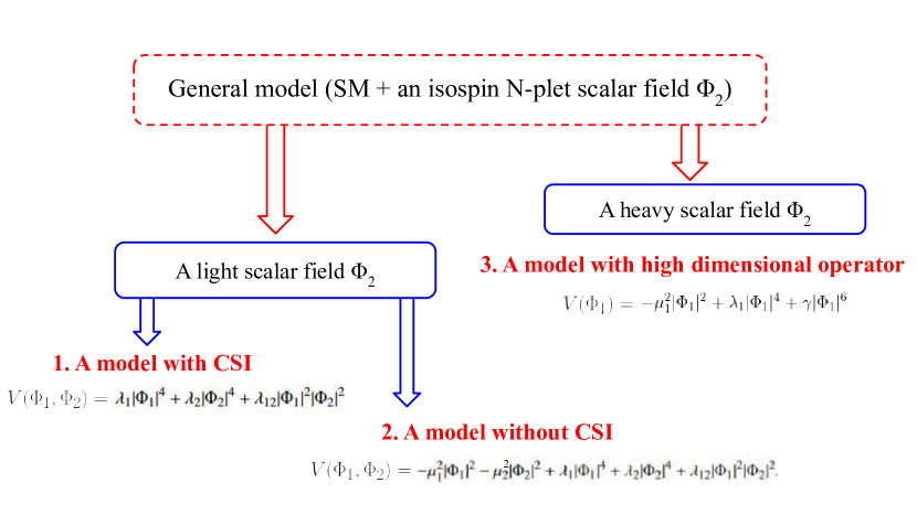
Figure 1: Our effective model description for some BSM models with FOPTs from a general model with an additional scalar field, which is either light or heavy consisting of (I) the light scalar model with CSI, (II) the light scalar model without CSI, (III) the heavy scalar model with high dimensional operator.

2.1 The model with classical scale invariance

In the first type of the model, we impose CSI on the tree-level potential without any dimensional parameters, then the spontaneous EWSB is generated by radiative corrections Coleman:1973jx given later in (24). The Lagrangian of this model is

$${\cal L}={\cal L}_{\mathrm{SM}}+\left|D_{\mu}\Phi_{2}\right|^{2}-V_{0}(\Phi_{1},\Phi_{2}),$$ (9)

where $D_{\mu}=\partial_{\mu}-igT^{a}W_{\mu}^{a}-ig^{\prime}Y_{\Phi_{2}}B_{\mu}/2$, $g^{\prime}$ and $g$ are U(1)_Y and SU(2)_I gauge couplings, respectively, and $T^{a}$ is the matrix for the generator of SU(2)_I. The tree-level potential $V_{0}(\Phi_{1},\Phi_{2})$ is given by

$$V_{0}(\Phi_{1},\Phi_{2})=\lambda_{1}|\Phi_{1}|^{4}+\lambda_{2}|\Phi_{2}|^{4}+\lambda_{12}|\Phi_{1}|^{2}|\Phi_{2}|^{2}.$$ (10)

If the isospin $I_{\Phi_{2}}$ is 1/2, then there are some mixing terms in the potential, such as $|\Phi_{1}^{\dagger}\Phi_{2}|^{2}$. For simplicity, we neglect such terms in the potential. According to Refs. Gildener:1976ih ; Endo:2015ifa , there may be a flat direction in the tree-level potential to assure the valid perturbative analysis. If not, the large logarithmic term may show up in the one-loop correction via the renormalization scale, for example, this scale in the $\phi^{4}$ theory is $Q\sim 3\lambda ve^{16\pi^{2}}$ Coleman:1973jx . Therefore we assume a flat direction in the tree-level potential to avoid invalidating the perturbative analysis. The details of the effective potential will be discussed in Sec. 3.

We mention here the current experimental constraints on this model. For simplicity, we assume that the additional scalar field $\Phi_{2}$ does not couple to the SM fermions and does not have the vacuum-expectation-value (VEV). On the other hand, the isospin $N$-plet scalar field $\Phi_{2}$ can interact with the SM gauge bosons. There are some experimental constraints on this model with respect to the gauge boson. The first one comes from the $\rho$ parameter, which is defined by

$$\rho_{0}=\frac{\sum_{i}\left[I_{i}(I_{i}+1)-Y_{i}^{2}\right]}{2\sum_{i}v_{i}^{2}Y_{i}^{2}}.$$ (11)

Here, the value at $2\sigma$ confidence level is  ParticleDataGroup:2018ovx

$$\rho_{0}=1.00039\pm 0.00019.$$ (12)

The new physics effects appear in two-point functions for weak gauge bosons, and we can use the precision measurements of the functions to explore the model beyond the SM. The corrections to them, which are called the oblique corrections, can be parameterized by $S$, $T$ and $U$ parameters Peskin:1990zt ; Peskin:1991sw . From the global fit of EW parameters, the values of $S$ and $T$ parameters under $U=0$ are given by  Zyla:2020zbs

$$S=0.00\pm 0.07,\quad T=0.05\pm 0.06.$$ (13)

The dominant new physics effects in the $h\gamma\gamma$ coupling is also one-loop level. The Higgs coupling $h\gamma\gamma$ is given by $1.05\pm 0.09$ ATLAS:2019nkf . Furthermore, the mass of charged scalar field should be larger than 155 GeV from charged Higgs boson searches Zyla:2020zbs . In our work, we do not take into account the experimental constraints in the numerical analysis of the PT.

2.2 The model without classical scale invariance

In the model without CSI, there are mass parameters in the tree-level potential. The tree-level potential in this model is given as

$$V_{0}(\Phi_{1},\Phi_{2})=-\mu_{1}^{2}|\Phi_{1}|^{2}-\mu_{2}^{2}|\Phi_{2}|^{2}+\lambda_{1}|\Phi_{1}|^{4}+\lambda_{2}|\Phi_{2}|^{4}+\lambda_{12}|\Phi_{1}|^{2}|\Phi_{2}|^{2},$$ (14)

where $\mu_{1}^{2}>0$ and $\lambda_{1},\lambda_{2}>0$ for the stability of the tree-level potential. The effective potential of this model will be given later in (47).

Before discussing the effective potential with loop-corrections, we show the possible PT paths from the tree-level potential. At first, the extremal values in the potential are obtained by

$$\frac{\partial V_{0}(\left\langle\Phi_{1}\right\rangle,\left\langle\Phi_{2}\right\rangle)}{\partial\left\langle\Phi_{1}\right\rangle}=\frac{\partial V_{0}(\left\langle\Phi_{1}\right\rangle,\left\langle\Phi_{2}\right\rangle)}{\partial\left\langle\Phi_{2}\right\rangle}=0,$$ (15)

which are solved by the following nine points in the field space as shown in Fig. 2,

$$\left(\left\langle\Phi_{1}\right\rangle,\left\langle\Phi_{2}\right\rangle\right)=(0,0),\quad \left(0,\pm\sqrt{\frac{\mu_{2}^{2}}{\lambda_{2}}}\right),\quad\left(\pm\sqrt{\frac{\mu_{1}^{2}}{\lambda_{1}}},0\right),$$

$$\left(\pm\sqrt{2\frac{\lambda_{12}\mu_{2}^{2}-2\lambda_{2}\mu_{1}^{2}}{\lambda_{12}^{2}-4\lambda_{1}\lambda_{2}}},\pm\sqrt{2\frac{\lambda_{12}\mu_{2}^{2}-2\lambda_{2}\mu_{1}^{2}}{\lambda_{12}^{2}-4\lambda_{1}\lambda_{2}}}\right), \left(\pm\sqrt{2\frac{\lambda_{12}\mu_{2}^{2}-2\lambda_{2}\mu_{1}^{2}}{\lambda_{12}^{2}-4\lambda_{1}\lambda_{2}}},\mp\sqrt{2\frac{\lambda_{12}\mu_{2}^{2}-2\lambda_{2}\mu_{1}^{2}}{\lambda_{12}^{2}-4\lambda_{1}\lambda_{2}}}\right).$$ (16)

The green point is the origin in the potential, the blue points are $\left\langle\Phi_{2}\right\rangle\not=0$ at zero temperature and red and magenta points are along $\left\langle\Phi_{1}\right\rangle$ and $\left\langle\Phi_{2}\right\rangle$ axes, respectively. To realize spontaneous EWSB at zero temperature, red or blue points are the minimum values. In this work, we especially focus on the one-step phase transition along $\left\langle\Phi_{1}\right\rangle$ axis, because this path is the same as the CSI case. We will compare differences of the results between the models with and without CSI.

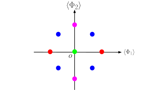
Figure 2: The extreme values of the tree-level potential given by Eq. (15).

2.3 The model with dimension-six operator from $\Phi_{2}$

In the last type of model, $\Phi_{2}$ is assumed at the TeV scale and then we integrate out the additional scalar field. The tree-level potential in this model is given by

$$V_{0}(\Phi_{1},\Phi_{2})=-\mu_{1}^{2}|\Phi_{1}|^{2}-\mu_{2}^{2}|\Phi_{2}|^{2}+\lambda_{1}|\Phi_{1}|^{4}+\lambda_{2}|\Phi_{2}|^{4}+\lambda_{12}|\Phi_{1}|^{2}|\Phi_{2}|^{2},$$ (17)

where $\mu_{2}$ is TeV scale. Otherwise it is the same as the model without CSI. Then, we integrate out the heavy $\Phi_{2}$ by loop-level matching Henning:2014wua ; Postma:2020toi in our analysis, and the effective Lagrangian for the SM-like Higgs boson $h$ reads

$${\cal L}_{\mathrm{EFT}}^{(6)}\sim\frac{1}{2}|\partial_{\mu}h|^{2}-\left(-\frac{1}{2}a_{2}h^{2}+\frac{1}{4}a_{4}h^{4}+\frac{1}{6}a_{6}h^{6}\right)$$ (18)

with

$$a_{2}=\mu_{1}^{2},\quad a_{4}=\lambda_{1}-(1+2I_{\Phi_{2}})\frac{\lambda_{12}^{2}\mu_{1}^{2}}{9(4\pi)^{2}m_{\Phi_{2}}^{2}},\quad a_{6}=(1+2I_{\Phi_{2}})\frac{1}{(4\pi)^{2}m_{\Phi_{2}}^{2}}\left(\frac{\lambda_{12}^{3}}{8}+\frac{\lambda_{12}^{2}\lambda_{1}}{6}\right),$$ (19)

where $m_{\Phi_{2}}^{2}=\mu_{2}^{2}+\lambda_{12}v^{2}/2$ is the mass of the additional scalar field $\Phi_{2}$. The effective potential with radiative corrections of this model is given later in (66).

We note that Ref. Postma:2020toi suggests FOPT may be difficult in the model with a loop-level matching. According to their work, the FOPT requires the balancing between the dimension-four and dimension-six terms via $\frac{1}{4}\frac{U}{M^{2}}\frac{c_{i}\kappa^{2}}{16\pi^{2}}\sim\frac{m_{h}^{2}}{v^{2}}\sim 0.12$ with $c_{i}$ = 1/2 (1) for a real (complex) scalar, where $U$ and $M$ correspond to the Higgs boson coupling to the heavy field and the mass parameter of heavy field, respectively. On the other hand, the parameter region for a valid EFT expansion requires $\frac{U}{M^{2}}\ll 1$ and $\frac{c_{i}\kappa^{2}}{16\pi^{2}}\ll 1$, therefore, they concluded that the FOPT cannot be generated in the model. However, the model has some scalar fields which contribute to the dimension-six term via the number of loop diagrams. Therefore, the FOPT can be realized in the parameter region which can satisfy the condition of a valid EFT expansion. At this time, we do not take into account other higher dimensional operators involving with the kinetic term. Such operators may contribute to the experimental constraints with respect to oblique parameters, like the Eq. (13).

3 Effective potentials

In this section, we discuss the forms of the effective potentials for our three effective model descriptions. To obtain the effective potential, we use the $\overline{\rm MS}$ scheme to absorb the divergence parts. Typically, the effective potential at one-loop level reads

$$V_{\rm eff}\left(\left\langle\Phi_{1}\right\rangle,\left\langle\Phi_{2}\right\rangle,T\right)=V_{0}+\sum_{i}\frac{n_{i}}{64\pi^{2}}\,M^{4}_{i}\left(\left\langle\Phi_{1}\right\rangle,\left\langle\Phi_{2}\right\rangle\right)\,\left(\ln\left(\frac{M^{2}_{i}\left(\left\langle\Phi_{1}\right\rangle,\left\langle\Phi_{2}\right\rangle\right)}{Q^{2}}\right)-c_{i}\right)+\Delta V_{T},$$ (20)

where $M^{2}_{i}\left(\left\langle\Phi_{1}\right\rangle,\left\langle\Phi_{2}\right\rangle\right)$ is the field-dependent mass, $n_{i}$ is the number of the degree of freedom, $Q$ is the renormalization scale and $c_{i}$ is 3/2 ($i=$ boson, fermion) or 5/6 ($i=$ gauge boson). The one-loop thermal contribution to the potential Dolan:1973qd is

$$\Delta V_{T} =\frac{T^{4}}{2\pi^{2}}\left\{\sum_{i={\rm bosons}}n_{i}\int_{0}^{\infty}dxx^{2}\ln\left[1-\exp\left(-\sqrt{x^{2}+M_{i}^{2}(\langle\Phi_{1}\rangle,\langle\Phi_{2}\rangle,T)/T^{2}}\right)\right]\right.$$

$$\left.+\sum_{i={\rm fermions}}n_{i}\int_{0}^{\infty}dxx^{2}\ln\left[1+\exp\left(-\sqrt{x^{2}+M_{i}^{2}(\langle\Phi_{1}\rangle,\langle\Phi_{2}\rangle,T)/T^{2}}\right)\right]\right\}.$$ (21)

Here, we take into account the resummation effect $V_{T}^{\rm ring}$ obtained by

$$V_{T}^{\rm ring}=\frac{T}{12\pi}\sum_{i=\rm bosons}n_{i}\left((M_{i}^{2}(\langle\Phi_{1}\rangle,\langle\Phi_{2}\rangle,T))^{3/2}-(M_{i}^{2}(\langle\Phi_{1}\rangle,\langle\Phi_{2}\rangle,T))^{3/2}\right),$$ (22)

where the thermal mass $M_{i}^{2}(\langle\Phi_{1}\rangle,\langle\Phi_{2}\rangle,T)=M_{i}^{2}(\langle\Phi_{1}\rangle,\langle\Phi_{2}\rangle)+\Pi_{i}$ receives the thermal correction from the thermal self-energy $\Pi_{i}$. Finally, the effective potential with finite temperature effects is obtained by

$$V_{\rm eff}\left(\left\langle\Phi_{1}\right\rangle,\left\langle\Phi_{2}\right\rangle,T\right)=V_{0}+V_{1-\rm loop}+\Delta V_{T}+V_{T}^{\rm ring}.$$ (23)

The field-dependent masses in the effective potential of Eq. (20) and thermal correction $\Pi_{i}$ in Eq. (23) depend on the details of model. Therefore we will discuss the form of effective potential in each type of the model in the following.

3.1 The model with classical scale invariance

For the model (10) with CSI, the spontaneous EWSB occurs on the flat direction, which is assumed along $\langle\Phi_{1}\rangle$. Then, the effective potential is simply

$$V_{\rm eff}(\varphi,T=0)=A\varphi^{4}+B\varphi^{4}\ln\frac{\varphi^{2}}{Q^{2}},$$ (24)

with $A$ and $B$ terms given by

$$A=\sum_{i}\frac{n_{i}}{64\pi^{2}v^{4}}m_{i}^{4}\left(\ln\frac{m_{i}^{2}}{v^{2}}-c_{i}\right),\quad B=\sum_{i}\frac{n_{i}}{64\pi^{2}v^{4}}m_{i}^{4},$$ (25)

where $m_{i}$ is the mass of the field species $i$ excluding the Higgs boson since this effect is at one-loop level in this model case. $n_{i}$ and $c_{i}$ in the potential are given by $(n_{W},n_{Z},n_{t},n_{\Phi_{2}})=(6,3,-12,2(2I_{\Phi_{2}}+1))$ and $(c_{W},c_{Z},c_{t})=(5/6,5/6,3/2,3/2)$, respectively. Using the stationary condition, we have

$$\left.\frac{\partial V_{\rm eff}(\varphi,T=0)}{\partial\varphi}\right|_{\varphi=v}=\ln\frac{v^{2}}{Q^{2}}+\frac{1}{2}+\frac{A}{B}=0,$$ (26)

where the renormalization scale $Q$ is fixed. Because $A$ and $B$ are the loop effects, $v$ can be large in contrast to the case of $\phi^{4}$ theory. Also, the Higgs boson mass is obtained as

$$m_{h}^{2}=\left.\frac{\partial^{2}V_{\rm eff}(\varphi,T=0)}{\partial\varphi^{2}}\right|_{\varphi=v}=8Bv^{2},$$ (27)

from which we can obtain the additional scalar boson mass $m_{\Phi_{2}}$ as

$$m_{\Phi_{2}}=\frac{C}{(2(2I_{\Phi_{2}}+1))^{1/4}},\quad C^{4}\equiv 8\pi^{2}v^{2}m_{h}^{2}-3m_{Z}^{4}-6m_{W}^{4}+12m_{t}^{4}$$ (28)

with $C=543\,\mathrm{GeV}$ determined by Eq.(10) of Hashino:2015nxa , and $\lambda_{12}$ coupling is obtained via relation $m_{\Phi_{2}}^{2}=\lambda_{12}v^{2}/2$ as

$$\lambda_{12}=\frac{\sqrt{2}C^{2}}{v^{2}\sqrt{2I_{\Phi_{2}}+1}}.$$ (29)

With the help of Eqs. (26) and (27), the one-loop effective potential at zero temperature could be obtained in terms of the renormalized mass of the Higgs boson as

$$V_{\rm eff}(\varphi,T=0)=\frac{m_{h}^{2}}{8v^{2}}\varphi^{4}\left(\ln\frac{\varphi^{2}}{v^{2}}-\frac{1}{2}\right).$$ (30)

Since the loop effects are renormalized into the Higgs boson mass, the value of $hhh$ coupling with one-loop effects does not depend on the model extension Hashino:2015nxa . The field-dependent masses and resummation effects in the effective potential with finite temperature effects are

$$M^{2}_{\Phi_{2}}(\varphi,T) =\frac{m^{2}_{\Phi_{2}}}{v^{2}}\varphi^{2}+T^{2}\left((I_{\Phi_{2}}+1)\frac{\lambda_{2}}{6}+\frac{m^{2}_{\Phi_{2}}}{3v^{2}}+I_{\Phi_{2}}(I_{\Phi_{2}}+1)\frac{g^{2}}{4}+Y_{\Phi_{2}}^{2}\frac{g^{\prime 2}}{16}\right).$$ (31)

Similarly, the thermally corrected field-dependent masses of gauge bosons in the ($W^{1},W^{2},W^{3},B$) basis are

$$M_{g}^{2(L,T)}(\varphi,T)=\frac{\varphi^{2}}{4}\left(\begin{array}[]{cccccccc}g^{2}&&&\\ &g^{2}&&\\ &&g^{2}&gg^{\prime}\\ &&gg^{\prime}&g^{\prime 2}\end{array}\right)+a_{g}^{(L,T)}T^{2}\left(\begin{array}[]{cccccccc}\pi_{W}&&&\\ &\pi_{W}&&\\ &&\pi_{W}&\\ &&&\pi_{B}\end{array}\right),$$ (40)

where

$$M_{W}^{2} =\frac{g^{2}}{4}\varphi^{2},\quad M_{WB}^{2}=\frac{gg^{\prime}}{4}\varphi^{2},\quad M_{B}^{2}=\frac{g^{\prime 2}}{4}\varphi^{2},$$ (41)

$$\pi_{W} =\frac{g^{2}}{9}I_{\Phi_{2}}\left(1+I_{\Phi_{2}}\right)\left(1+2I_{\Phi_{2}}\right)+\frac{11}{6}g^{2},$$ (42)

$$\pi_{B} =\frac{g^{\prime 2}T^{2}}{12}\left(1+I_{\Phi_{2}}\right)Y_{\Phi_{2}}^{2}+\frac{11}{6}g^{\prime 2},\quad a^{L}_{g}=1,\quad a^{T}_{T}=0.$$ (43)

The field-dependent mass of fermion does not receive thermal correction in $T^{2}$ so that

$$M_{t}^{2} =\frac{m_{t}^{2}}{v^{2}}\varphi^{2}.$$ (44)

In this model, there are three parameters in the tree-level potential,

$$\lambda_{1},\lambda_{2},\lambda_{12},$$ (45)

where $\lambda_{1}$ is zero in order to assume a flat direction along $\langle\Phi_{1}\rangle$ axis. According to Eq. (27), the isospin number $I_{\Phi_{2}}$ is related to the mass $m_{\Phi_{2}}$. Therefore, the free parameters in the effective potential with finite temperature effects are in fact

$$I_{\Phi_{2}},Y_{\Phi_{2}},\lambda_{2}.$$ (46)

3.2 The model without classical scale invariance

For the model (14) without CSI, the effective potential is given by

$$V_{\rm eff}\left(\varphi_{1},\varphi_{2},T\right)=V_{0}+\sum_{i}\frac{n_{i}}{64\pi^{2}}\,M^{4}_{i}\,\left(\ln\frac{M^{2}_{i}}{Q^{2}}-c_{i}\right)+\Delta V_{T},$$ (47)

where $\left\langle\Phi_{1}\right\rangle=\varphi_{1}/\sqrt{2}$, $\left\langle\Phi_{2}\right\rangle=\varphi_{2}/\sqrt{2}$ and

$$V_{0}=-\frac{\mu_{1}^{2}}{2}\varphi_{1}^{2}-\frac{\mu_{2}^{2}}{2}\varphi_{2}^{2}+\frac{\lambda_{1}}{4}\varphi_{1}^{4}+\frac{\lambda_{2}}{4}\varphi_{2}^{4}+\frac{\lambda_{12}}{4}\varphi_{1}^{2}\varphi^{2}_{2}.$$ (48)

There are the five model parameters in the tree-level potential and these parameters can be fixed in terms of following parameters,

$$v,m_{h},m_{\Phi_{2}},\lambda_{12},\lambda_{2},$$ (49)

by the stationary conditions and the second derivatives of the effective potential. The details of them are given in Appendix A.

The field-dependent masses with resummation corrections from the finite temperature effects of the effective potential are

$$M^{2}_{h,\Phi_{2}}(\varphi_{1},\varphi_{2},T)= \frac{1}{2}\left(M_{11}^{2}+M_{22}^{2}\mp\sqrt{(M_{11}^{2}-M_{22}^{2})^{2}+4M_{12}^{2}M_{21}^{2}}\right),$$ (50)

$$M^{2}_{N_{1}}(\varphi_{1},\varphi_{2},T)= -\mu_{1}^{2}+\lambda_{1}\varphi_{1}^{2}+\frac{\lambda_{12}}{2}\varphi_{2}^{2}$$

$$+T^{2}\left((2I_{\Phi_{2}}+1)\frac{\lambda_{12}}{12}+\frac{\lambda_{h}}{4}+\frac{3g^{2}}{16}+\frac{g^{\prime 2}}{16}+\frac{y_{t}^{2}}{4}\right),$$ (51)

$$M^{2}_{N_{2}}(\varphi_{1},\varphi_{2},T)= -\mu_{2}^{2}+\lambda_{2}\varphi_{2}^{2}+\frac{\lambda_{12}}{2}\varphi_{1}^{2}$$

$$+T^{2}\left(\frac{(I_{\Phi_{2}}+1)\lambda_{2}}{6}+\frac{\lambda_{12}}{6}+\frac{g^{2}}{4}\left(I_{\Phi_{2}}^{2}+I_{\Phi_{2}}\right)+\frac{g^{\prime 2}Y_{\Phi_{2}}^{2}}{16}\right),$$ (52)

where

$$\begin{pmatrix}M_{11}^{2}&M_{12}^{2}\\ M_{21}^{2}&M_{22}^{2}\end{pmatrix}=\begin{pmatrix}-\mu_{1}^{2}+3\lambda_{1}\varphi_{1}^{2}+\frac{\lambda_{12}}{2}\varphi_{2}^{2}&\lambda_{12}\varphi_{1}\varphi_{2}\\ \lambda_{12}\varphi_{1}\varphi_{2}&-\mu_{2}^{2}+3\lambda_{2}\varphi_{2}^{2}+\frac{\lambda_{12}}{2}\varphi_{1}^{2}\end{pmatrix}$$

$$\quad+T^{2}\begin{pmatrix}(2I_{\Phi_{2}}+1)\frac{\lambda_{12}}{12}+\frac{\lambda_{1}}{4}+\frac{3g^{2}}{16}+\frac{g^{\prime 2}}{16}+\frac{y_{t}^{2}}{4}&0\\ 0&\frac{(I_{\Phi_{2}}+1)\lambda_{2}}{6}+\frac{\lambda_{12}}{6}+\frac{g^{2}}{4}\left(I_{\Phi_{2}}^{2}+I_{\Phi_{2}}\right)+\frac{g^{\prime 2}Y_{\Phi_{2}}^{2}}{16}\end{pmatrix}.$$ (53)

Also the thermally corrected field-dependent masses of gauge bosons in the ($W^{1},W^{2},W^{3},B$) basis are

$$M_{g}^{2(L,T)}=\left(\begin{array}[]{cccccccc}M_{W}^{2}&&&\\ &M_{W}^{2}&&\\ &&M_{W}^{2}&M_{WB}^{2}\\ &&M_{WB}^{2}&M_{B}^{2}\end{array}\right)+a_{g}^{(L,T)}T^{2}\left(\begin{array}[]{cccccccc}\pi_{W}&&&\\ &\pi_{W}&&\\ &&\pi_{W}&\\ &&&\pi_{B}\end{array}\right),$$ (62)

where

$$M_{W}^{2} =\frac{g^{2}}{4}\left(\varphi_{1}^{2}+I_{W}^{2}\varphi_{2}^{2}\right),\quad M_{WB}^{2}=\frac{gg^{\prime}}{4}\left(\varphi_{1}^{2}+Y_{\Phi_{2}}^{2}\varphi_{2}^{2}\right),$$ (63)

$$M_{B}^{2} =\frac{g^{\prime 2}}{4}\left(\varphi_{1}^{2}+Y_{\Phi_{2}}^{2}\varphi_{2}^{2}\right),\quad\pi_{W}=\frac{g^{2}}{9}I_{\Phi_{2}}\left(1+I_{\Phi_{2}}\right)\left(1+2I_{\Phi_{2}}\right)+\frac{11}{6}g^{2},$$ (64)

$$\pi_{B} =\frac{g^{\prime 2}T^{2}}{12}\left(1+I_{\Phi_{2}}\right)Y_{\Phi_{2}}^{2}+\frac{11}{6}g^{\prime 2},\quad a^{L}_{g}=1,\quad a^{T}_{T}=0.$$ (65)

In this model, the EWPT can be generated in multi-field space $(\varphi_{1},\varphi_{2})$. We will focus on the path of the phase transition along $\varphi_{1}$ axis.

3.3 The model with dimension-six operator from $\Phi_{2}$

For the effective model (18) after integrating out the heavy scalar sector from (17), the effective potential is

$$V_{\rm eff}\left(\varphi_{1},T\right)=-\frac{1}{2}a_{2}\varphi_{1}^{2}+\frac{1}{4}a_{4}\varphi_{1}^{4}+\frac{1}{6}a_{6}\varphi_{1}^{6}+\sum_{i}\frac{n_{i}}{64\pi^{2}}\,M^{4}_{i}\,\left(\ln\left(\frac{M^{2}_{i}}{Q^{2}}\right)-c_{i}\right)+\Delta V_{T},$$ (66)

where $a_{2}$, $a_{4}$ and $a_{6}$ are given in Eq. (19), and the field-dependent mass of Higgs boson along with its thermal correction are

$$M_{h}^{2}(\varphi_{1})=-a_{2}+3a_{4}\varphi_{1}^{2}+5a_{6}\varphi_{1}^{4},\quad\Pi_{h}=T^{2}\left(\frac{a_{4}}{4}+\frac{3g^{2}}{16}+\frac{g^{\prime 2}}{16}+\frac{y_{t}^{2}}{4}\right).$$ (67)

The thermally corrected field-dependent masses of gauge bosons in the ($W^{1},W^{2},W^{3},B$) basis are

$$M_{g}^{2(L,T)}(\varphi,T)=\frac{\varphi^{2}}{4}\left(\begin{array}[]{cccccccc}g^{2}&&&\\ &g^{2}&&\\ &&g^{2}&gg^{\prime}\\ &&gg^{\prime}&g^{\prime 2}\end{array}\right)+a_{g}^{(L,T)}T^{2}\left(\begin{array}[]{cccccccc}\pi_{W}&&&\\ &\pi_{W}&&\\ &&\pi_{W}&\\ &&&\pi_{B}\end{array}\right),$$ (76)

where

$$M_{W}^{2} =\frac{g^{2}}{4}\varphi_{1}^{2},\quad M_{WB}^{2}=\frac{gg^{\prime}}{4}\varphi_{1}^{2},\quad M_{B}^{2}=\frac{g^{\prime 2}}{4}\varphi_{1}^{2},$$ (77)

$$\pi_{W} =\frac{11}{6}g^{2},\quad\pi_{B}=\frac{11}{6}g^{\prime 2},\quad a^{L}_{g}=1,\quad a^{T}_{T}=0$$ (78)

and the field-dependent mass of top quark is

$$M_{t}^{2} =\frac{m_{t}^{2}}{v^{2}}\varphi_{1}^{2}.$$ (79)

There are three new parameters in this potential, namely,

$$m_{\Phi_{2}}^{2},\lambda_{12},I_{\Phi_{2}}.$$ (80)

4 Gravitational waves

The GWs from the FOPTs serve as the promising probe for the new physics of BSM, including our EFT models of EWSB. Although the paradigm of GWs from FOPTs has been extensively described in the literatures for concrete model buildings, we include here some recent new progress.

4.1 Phase-transition dynamics

For an effective potential $V_{\mathrm{eff}}$ exhibiting a false vacuum $\phi_{+}$ and a true vacuum $\phi_{-}$ separated by a potential barrier, a cosmological FOPT proceeds via stochastic nucleations of true vacuum bubbles followed by a rapid expansion until a successful percolation to fully complete the phase transition process. In this section, we describe the phase transition dynamics consisting of the bubble nucleation and bubble percolation, which could be determined by the thermodynamics of effective potential alone without reference to the microscopic physics that leads to the macroscopic hydrodynamics of bubble expansion.

Bounce action

The bubble nucleations of true vacuum bubbles at finite temperature admit stochastic emergences of the field configuration $\phi(r)$ connecting a true vacuum region $\phi(r=0)\equiv\phi_{0}\lesssim\phi_{-}$ (assuming $\phi_{+}<\phi_{-}$) to the asymptotic false vacuum region $\phi(r\to\infty)\equiv\phi_{+}$ in an $O(4)$-symmetric manner $\mathrm{d}s^{2}=\mathrm{d}r^{2}+r^{2}\mathrm{d}\Omega_{3}^{2}$ or an $O(3)$-symmetric manner $\mathrm{d}s^{2}=\mathrm{d}\tau^{2}+\mathrm{d}r^{2}+r^{2}\mathrm{d}\Omega_{2}^{2}$ depending on their maximum value of the nucleation rates Coleman:1977py ; Callan:1977pt ; Linde:1980tt ; Linde:1981zj

$$\Gamma(T)=\max\left[T^{4}\left(\frac{S_{3}}{2\pi T}\right)^{\frac{3}{2}}e^{-\frac{S_{3}}{T}},\frac{1}{R_{0}^{4}}\left(\frac{S_{4}}{2\pi}\right)e^{-S_{4}}\right],$$ (81)

where the $O(4)$ bounce action

$$S_{4}=2\pi^{2}\int_{0}^{\infty}\mathrm{d}r\,r^{3}\left[\frac{1}{2}\left(\frac{\mathrm{d}\phi_{B}}{\mathrm{d}r}\right)^{2}+V_{\mathrm{eff}}(\phi_{B},T)-V_{\mathrm{eff}}(\phi_{+},T)\right]$$ (82)

is evaluated at the solution $\phi_{B}$ of the equation-of-motion

$$\frac{\mathrm{d}^{2}\phi}{\mathrm{d}r^{2}}+\frac{3}{r}\frac{\mathrm{d}\phi}{\mathrm{d}r}=\frac{\partial V_{\mathrm{eff}}}{\partial\phi},\quad\phi^{\prime}(0)=0,\quad\phi(\infty)=\phi_{+},$$ (83)

while the $O(3)$ bounce action

$$\frac{S_{3}}{T}=\frac{4\pi}{T}\int_{0}^{\infty}\mathrm{d}r\,r^{2}\left[\frac{1}{2}\left(\frac{\mathrm{d}\phi_{B}}{\mathrm{d}r}\right)^{2}+V_{\mathrm{eff}}(\phi_{B},T)-V_{\mathrm{eff}}(\phi_{+},T)\right]$$ (84)

is evaluated at the solution $\phi_{B}$ of the equation-of-motion

$$\frac{\mathrm{d}^{2}\phi}{\mathrm{d}r^{2}}+\frac{2}{r}\frac{\mathrm{d}\phi}{\mathrm{d}r}=\frac{\partial V_{\mathrm{eff}}}{\partial\phi},\quad\phi^{\prime}(0)=0,\quad\phi(\infty)=\phi_{+}.$$ (85)

In the realistic estimations, the vacuum decay rate from $S_{4}$ usually dominates over the thermal decay rate from $S_{3}/T$ at extremely low temperature when the potential barrier does not vanish even at $T=0$. $R_{0}$ is the bubble radius defined by $\phi_{B}(r=R_{0})=(\phi_{0}-\phi_{+})/2$.

Nucleation temperature

During the whole process of bubble nucleation, the false vacuum becomes unstable once the temperature drops below the critical temperature defined by

$$V_{\mathrm{eff}}(\phi_{+},T_{c})=V_{\mathrm{eff}}(\phi_{-}(T_{c}),T_{c}).$$ (86)

However, the bubble nucleation is only possible when the temperature further drops down to $T=T_{i}<T_{c}$ defined

$$\phi_{B}(r=0,T_{i})=\phi_{-}(T_{i})$$ (87)

due to the presence of the Hubble friction term in the bounce equation. Since then, one can count the number of nucleated bubbles in one Hubble volume during a given time elapse by

$$N(T(t))=\int_{t_{i}}^{t}\mathrm{d}t\frac{\Gamma(t)}{H^{3}}=\int_{T}^{T_{i}}\frac{\mathrm{d}T}{T}\frac{\Gamma(T)}{H(T)^{4}},$$ (88)

until the nucleation temperature $T_{n}<T_{i}$ defined by the moment when there is exactly one bubble nucleated in one Hubble volume,

$$N(T_{n})=1.$$ (89)

In the realistic estimations, the exponential part of bounce action dominates the integral in $N(T)$, therefore, a rough estimation from

$$\frac{\Gamma(T)}{H(T)^{4}}=\frac{T^{4}}{H(T)^{4}}\left(\frac{S_{3}}{2\pi T}\right)^{\frac{3}{2}}e^{-S_{3}/T}=\left(\frac{90}{\pi^{2}g_{\mathrm{dof}}}\right)^{2}\frac{M_{\mathrm{Pl}}^{4}}{T^{4}}\left(\frac{S_{3}}{2\pi T}\right)^{\frac{3}{2}}e^{-S_{3}/T}=1$$ (90)

gives rise to a thumb rule

$$\frac{S_{3}}{T}=4\log\frac{M_{\mathrm{Pl}}}{T}+\frac{3}{2}\log\frac{S_{3}}{2\pi T}+2\log\frac{90}{\pi^{2}g_{\mathrm{dof}}}\approx 4\log\frac{M_{\mathrm{Pl}}}{T}\approx 130\sim 140$$ (91)

for the EWPTs with $T\sim\mathcal{O}(100)$ GeV, which, however, will not be used here for the characteristic temperature of the phase transition.

Percolation temperature

The progress of the phase transition could be described by the the expected volume fraction of the true-vacuum regions at time $t$ Guth:1982pn ; Turner:1992tz ; Ellis:2018mja ,

$$I(t)=\frac{4\pi}{3}\int_{t_{i}}^{t}\mathrm{d}t^{\prime}\,\Gamma(t^{\prime})a(t^{\prime})^{3}r(t,t^{\prime})^{3},$$ (92)

where $r(t,t^{\prime})$ is the comoving radius of a bubble at $t$ nucleated at an earlier time $t^{\prime}$,

$$r(t,t^{\prime})\equiv\frac{R_{0}}{a(t^{\prime})}+\int_{t^{\prime}}^{t}\frac{v_{w}(\tilde{t})\mathrm{d}\tilde{t}}{a(\tilde{t})}\approx v_{w}\int_{t^{\prime}}^{t}\frac{\mathrm{d}\tilde{t}}{a(\tilde{t})}.$$ (93)

Here we omit the initial bubble radius $R_{0}$ and fix the time-dependent bubble wall velocity $v_{w}(t)$ at its terminal $v_{w}$. When the effects for the overlapping of true-vacuum bubbles and “virtual bubbles” nucleated in the true-vacuum regions are taken into account, the fraction of regions that are still sitting at the false vacuum at time $t$ could be approximated by the exponentiation of $I(t)$,

$$P(t)=e^{-I(t)}.$$ (94)

A percolation temperature $T_{p}<T_{n}$ is therefore defined by a conventional estimation Leitao:2012tx ; Leitao:2015fmj ; Ellis:2018mja ; Ellis:2020awk ; Wang:2020jrd

$$P(T_{p})=1/e.$$ (95)

However, sine the background is also expanding, a successful achievement of $P(T_{p})=1/e$ does not necessarily lead to a successful completion of the phase transition. A necessary (but not sufficient) condition for the phase transition completion is a decreasing trend for the physical volumes $\mathcal{V}_{\mathrm{phys}}\propto a(t)^{3}P(t)$ of the false-vacuum regions Guth:1982pn ; Turner:1992tz ; Ellis:2018mja ,

$$\frac{1}{\mathcal{V}_{\mathrm{phys}}}\frac{\mathrm{d}\mathcal{V}_{\mathrm{phys}}}{\mathrm{d}t}=3H(t)-\frac{\mathrm{d}I(t)}{\mathrm{d}t}=H(T)\left(3+T\frac{\mathrm{d}I(T)}{\mathrm{d}T}\right)<0.$$ (96)

Along with the bubble percolation to successfully complete the phase transition, a reheating process is required to bring the Universe at a non-equilibrium state into a thermal equilibrium again at Ellis:2018mja

$$T_{\mathrm{reh}}\simeq T_{p}\left[1+\alpha(T_{p})\right]^{\frac{1}{4}},$$ (97)

which is obtained from evaluating the radiation energy density after PT by

$$\rho_{\mathrm{rad}}(t>t_{\mathrm{PT}}) \equiv\frac{\pi^{2}}{30}g_{\mathrm{eff}}T_{\mathrm{reh}}^{4}=\rho_{\mathrm{rad}}(t\leq t_{\mathrm{PT}})+(1-\kappa_{\phi}-\kappa_{v})\alpha\rho_{\mathrm{rad}}(t\leq t_{\mathrm{PT}})$$

$$\approx(1+\alpha)\rho_{\mathrm{rad}}(t\leq t_{\mathrm{PT}})=\frac{\pi^{2}}{30}g_{\mathrm{eff}}(1+\alpha)T_{p}^{4}.$$ (98)

Here the strength factor $\alpha$, the efficiency factors $\kappa_{\phi}$ and $\kappa_{v}$ from the bubble wall motion and bulk fluid motion, respectively, are defined later. In the realistic estimations, the characteristic temperature of PT is defined by $T_{*}\simeq T_{\mathrm{reh}}$, and we will simply take $T_{*}=T_{p}$.

Strength factor

In the last equation, the parameter $\alpha$ is defined to characterize the total released latent heat into the plasma by Ellis:2018mja

$$\alpha(T)=\frac{\Delta\rho_{\mathrm{vac}}(T)}{\rho_{\mathrm{rad}}(T)},$$ (99)

with the total released vacuum energy defined by

$$\Delta\rho_{\mathrm{vac}}(T)=\rho(\phi_{+},T)-\rho(\phi_{-}(T),T)=\Delta V_{\mathrm{eff}}(T)-T\frac{\partial\Delta V_{\mathrm{eff}}(T)}{\partial T}$$ (100)

due to $\rho=\mathcal{F}+Ts=-p+T\frac{\partial p}{\partial T}=V_{\mathrm{eff}}-T\frac{\partial V_{\mathrm{eff}}}{\partial T}$ similar to the usual definition of latent heat $L(T_{c})=\rho(\phi_{+},T_{c})-\rho(\phi_{-}(T_{c}),T_{c})$ at critical temperature. Here $\Delta V_{\mathrm{eff}}(T)\equiv V_{\mathrm{eff}}(\phi_{+}(T),T)-V_{\mathrm{eff}}(\phi_{-}(T),T)$ for short. Note that for the strong FOPT with detonation expansion ($v_{w}>v_{J}>c_{s}$ defined later), the latent heat released in front of the bubble wall, $\alpha_{+}$, simply equals to its asymptotic value, $\alpha_{N}$, while for the weak FOPT with deflagration expansion ($v_{w}<c_{s}$ defined later), the latent heat released just in front of the bubble wall is disturbed by the shockwaves that obscures the definition of $\alpha$. In this study, we will only consider the case with relatively large bubble wall velocity $v_{w}\gg c_{s}$ without reference to the difference between $\alpha_{+}$ and $\alpha_{N}$, and use the same symbol $\alpha$ for the strength of phase transition.

It is worth noting that there is another definition of the strength factor with a factor of 4 difference,

$$\alpha_{0}(T)\equiv\frac{1}{\rho_{\mathrm{rad}}(T)}\left[\Delta V_{\mathrm{eff}}(T)-\frac{T}{4}\frac{\partial\Delta V_{\mathrm{eff}}(T)}{\partial T}\right],$$ (101)

which is motivated by the bag approximation for the equation of state (EOS) of the scalar-plasma system. The key observation for the bag EOS is that the finite temperature part of the effective potential $V_{T}\equiv V_{\mathrm{eff}}^{T\neq 0}$ at the massless and large massive limits for the coupled particles could be approximated by

$$V_{T}(\phi,T)=\sum\limits_{i=B,F}\pm g_{i}T\int\frac{\mathrm{d}^{3}\vec{k}}{(2\pi)^{3}}\log\left(1\mp e^{-\frac{\sqrt{k^{2}+m_{i}^{2}(\phi)}}{T}}\right)\approx\begin{cases}-\frac{\rho_{\mathrm{rad}}(T)}{3},&m_{i}\ll T,\\ 0,&m_{i}\gg T,\end{cases}$$ (102)

which is the case for no particle gaining mass comparable to the temperature, $m_{i}\approx T$, during the penetration across the bubble wall. Since the massive heavy particles have no contribution to the radiation

$$\rho_{\mathrm{rad}}(T)=\frac{\pi^{2}}{30}g_{\mathrm{eff}}T^{4},\quad g_{\mathrm{eff}}=\sum\limits_{i=B}g_{i}+\frac{7}{8}\sum\limits_{i=F}g_{i},\quad m_{i}\ll T,$$ (103)

the pressure and energy density for the scalar-plasma system simply read

$$p_{\pm}(T) =-V_{\mathrm{eff}}(\phi_{\pm}(T),T)\approx\frac{1}{3}\rho_{\mathrm{rad}}^{\pm}(T)-V_{0}(\phi_{\pm}),$$ (104)

$$\rho_{\pm}(T) =V_{\mathrm{eff}}(\phi_{\pm}(T),T)-T\frac{\partial}{\partial T}V_{\mathrm{eff}}(\phi_{\pm}(T),T)\approx\rho_{\mathrm{rad}}^{\pm}(T)+V_{0}(\phi_{\pm}),$$ (105)

where in the last approximation we have ignored the mild dependence on $T$ in $\phi_{\pm}(T)$ for the zero-temperature part of the effective potential $V_{0}\equiv V_{\mathrm{eff}}^{T=0}$. Hence the sound speed reads $c_{s,\pm}^{2}=\partial p_{\pm}/\partial\rho_{\pm}=1/3$ in both symmetric and broken phases. This bag EOS renders the vacuum part of the effective potential as

$$V_{0}(\phi_{\pm})=\frac{1}{4}(\rho_{\pm}-3p_{\pm})=V_{\mathrm{eff}}(\phi_{\pm},T)-\frac{T}{4}\frac{\partial}{\partial T}V_{\mathrm{eff}}(\phi_{\pm},T),$$ (106)

where the temperature-dependence at right-hand-side implicitly cancels out to yield a temperature-independence at left-hand-side. Therefore, the strength factor defined in (101) for the bag EOS simply accounts for the pure difference in the vacuum part of effective potential (hence with subscript “0” in $\alpha_{0}$),

$$\alpha_{0}(T)=\frac{V_{0}(\phi_{+})-V_{0}(\phi_{-})}{\rho_{\mathrm{rad}}(T)}.$$ (107)

We will not use this definition of the strength factor for calculations since the finite temperature part of the effective potential seems to contribute nothing to $\alpha_{0}$. Note that the strength factor definition (101) could also be generalized beyond the bag EOS with a temperature-dependent sound speed as Hindmarsh:2017gnf

$$\alpha_{\theta}(T)=\frac{1}{3\omega_{+}(T)}\left[\left(1+\frac{1}{c_{s}(T)^{2}}\right)\Delta V_{\mathrm{eff}}(T)-T\frac{\partial}{\partial T}\Delta V_{\mathrm{eff}}(T)\right]\equiv\frac{\theta_{+}(T)-\theta_{-}(T)}{3\omega_{+}(T)},$$ (108)

where the prefactor $\omega_{+}$ is the enthalpy density $\omega=\rho+p=-T\partial V_{\mathrm{eff}}/\partial T$ in the symmetric phase, and $\theta\equiv\rho-p/c_{s}^{2}$ is the trace anomaly. We will also not use this definition for calculations since we have no plan to go beyond the bag EOS in the current investigation.

Characteristic length scale

Another characteristic parameter is the length scale of the bubble radius at collisions Ellis:2018mja ,

$$R_{*}=R_{\mathrm{max}},$$ (109)

corresponding to the peak frequency of the GW energy density spectrum from bubble wall collisions (defined later), where $R_{\mathrm{max}}$ maximizes the energy distribution

$$\mathcal{E}(R,t;t_{R})=R^{3}\frac{\mathrm{d}n}{\mathrm{d}R}(R,t;t_{R})$$ (110)

with the distribution of bubble sizes at temperature $T$ estimated by

$$\frac{\mathrm{d}n}{\mathrm{d}R}(R,t;t_{R})=-\frac{\mathrm{d}t_{R}}{\mathrm{d}R}\left(\frac{a(t_{R})}{a(t)}\right)^{3}P(t_{R})\Gamma(t_{R}).$$ (111)

Here $R$ is the bubble radius at $T$ that is nucleated at an earlier time $t_{R}$,

$$R\equiv R(t,t_{R})=a(t)r(t,t_{R})=2\sqrt{t}(\sqrt{t}-\sqrt{t_{R}})=\frac{2\xi}{T}\left(\frac{1}{T}-\frac{1}{T_{R}}\right)$$ (112)

with $\xi^{2}\equiv 45M_{\mathrm{Pl}}^{2}/2\pi^{2}g_{\mathrm{dof}}$, $g_{\mathrm{dof}}=106.75$, $M_{\mathrm{Pl}}^{2}\equiv 1/8\pi G_{\mathrm{N}}$. The sound wave contribution to the GW energy density spectrum corresponds to the width of sound shell Ellis:2018mja ,

$$R_{*}=(v_{w}-c_{s})R_{\mathrm{max}}.$$ (113)

A more efficient estimation for $R_{*}$ comes from the duration of the phase transition with exponential nucleation rate

$$\Gamma=e^{\beta_{1}(t-t_{p})+\cdots},\quad P(t_{p})=1/e,\quad\beta_{1}=\left.-\frac{\mathrm{d}}{\mathrm{d}t}\frac{S_{3}(t)}{T(t)}\right|_{t=t_{p}}=\left.H(T)T\frac{\mathrm{d}}{\mathrm{d}T}\frac{S_{3}(T)}{T}\right|_{T=T_{p}}$$ (114)

or simultaneous nucleation rate

$$\Gamma=e^{-\frac{1}{2}\beta_{2}(t-t_{m})^{2}+\cdots},\quad\left.\frac{\mathrm{d}}{\mathrm{d}t}\frac{S_{3}}{T}\right|_{t=t_{m}}=0,\quad\beta_{2}=\left.\sqrt{\frac{\mathrm{d}^{2}}{\mathrm{d}t^{2}}\frac{S_{3}}{T}}\right|_{t=t_{m}}=H(T)T\left.\sqrt{\frac{\mathrm{d}^{2}}{\mathrm{d}T^{2}}\frac{S_{3}}{T}}\right|_{T=T_{m}},$$ (115)

where in the former case it is related to the average number density by

$$n_{B}=R_{*}^{-3}=\frac{1}{8\pi}\left(\frac{\beta_{1}}{v_{w}}\right)^{3},$$ (116)

while in the later case it is related to the averaged number density by

$$n_{B}=R_{*}^{-3}=\sqrt{2\pi}\frac{\Gamma(T_{m})}{\beta_{2}}.$$ (117)

4.2 Bubble-expansion dynamics

Besides the input from the thermodynamics of the effective potential, the bubble-expansion dynamics involves both microscopic particle physics and macroscopic hydrodynamics, which give rise to the efficiency factors of transforming the total released vacuum energy into the bubble wall motion and bulk fluid motion.

The efficiency factor of the bubble wall motion

The microscopic particle physics determines the specific form of the thermal friction term

$$\delta f=\sum\limits_{i=\mathrm{B,F}}g_{i}\frac{\mathrm{d}m_{i}^{2}}{\mathrm{d}\phi}\int\frac{\mathrm{d}^{3}\vec{k}}{(2\pi)^{3}}\frac{\delta f_{i}}{2E_{i}(\vec{k})}$$ (118)

in the combined Boltzmann equations

$$\square\phi-\frac{\partial V_{\mathrm{eff}}}{\partial\phi} =\delta f;$$ (119)

$$\partial_{\mu}T_{\mathrm{p}}^{\mu\nu}+\partial^{\nu}\phi\frac{\partial V_{T}}{\partial\phi} =-\partial^{\nu}\phi\cdot\delta f,$$ (120)

where $V_{T}$ is the finite-temperature part of the effective potential, and the friction term $\delta f$ characterizes the deviations from the thermal equilibrium $f_{i}=f_{i}^{\mathrm{eq}}+\delta f_{i}$. Since we are dealing with the effective benchmark models that are not confined to a specific particle physics model, there is no universal form for the friction term $\delta f$. However, some model-independent phenomenological parameterizations are proposed, for example, in Ignatius:1993qn ; Megevand:2009ut ; Megevand:2009gh with a form of

$$\delta f=\eta_{T}u^{\mu}\partial_{\mu}\phi,$$ (121)

and in Cai:2020djd with a form of

$$\delta f=-\tilde{\eta}_{T}(u^{\mu}\partial_{\mu}\phi)^{2}.$$ (122)

The difference of above two forms of the friction term is that, when integrating the scalar equation-of-motion (119) in the vicinity of bubble wall, the derived effective equation-of-motion of the bubble wall position $R(t)$ Cai:2020djd ,

$$\left(\sigma+\frac{R}{3}\frac{\mathrm{d}\Delta p_{\mathrm{fr}}}{\mathrm{d}\gamma}\right)\gamma^{3}\ddot{R}+\frac{2\sigma\gamma}{R}=\Delta p_{\mathrm{dr}}-\Delta p_{\mathrm{fr}},$$ (123)

exhibits different forms of the friction force term $\Delta p_{\mathrm{fr}}\equiv\Delta p_{\mathrm{LO}}+h(\gamma)\Delta p_{N\mathrm{LO}}$ for the interactions between the bubble wall and thermal plasma. Here $\gamma=1/\sqrt{1-\dot{R}^{2}}$ is the Lorentz factor of the moving bubble wall, and the driving force $\Delta p_{\mathrm{dr}}=V_{\mathrm{eff}}(\phi_{+})-V_{\mathrm{eff}}(\phi_{-})$ is driven by the potential difference between the false and true vacuums. The leading-order friction force $\Delta p_{\mathrm{LO}}$ from the particle transmission/reflection $P_{1\to 1}\approx\Delta m^{2}T^{2}/24$ Bodeker:2009qy is independent of the $\gamma$ factor. The next-to-leading-order friction force $\gamma\Delta p_{\mathrm{NLO}}$ from the transition splitting $P_{1\to 2}\approx\gamma g^{2}\Delta m_{V}T^{3}$ Bodeker:2017cim admits a linear dependence on the $\gamma$-factor, which could be obtained from the friction term parameterization (121). The all orders friction force $\gamma^{2}\Delta p_{N\mathrm{LO}}$ Hoeche:2020rsg admits a quadratic dependence on the $\gamma$-factor, similar to a thermodynamic considerations $\Delta p=(\gamma^{2}-1)T\Delta s$ Mancha:2020fzw , which could be reproduced from the friction term parameterization (122).

Without reference to the microscopic physics, we parameterize the friction force with arbitrary $h(\gamma)$. The effective equation-of-motion (123) can be solved directly with a solution $\gamma(R)$ satisfying following algebraic equation Cai:2020djd ,

$$\frac{h(\gamma)-h(1)}{h(\gamma_{\mathrm{eq}})-h(1)}+\frac{3\gamma}{2R}=1+\frac{1}{2R^{3}}$$ (124)

which renders the total energy $E=4\pi R^{2}\sigma\gamma-\frac{4}{3}\pi R^{3}(\Delta p_{\mathrm{dr}}-\Delta p_{\mathrm{fr}})$ conserved during the bubble expansion. Here $R$ is already normalized by the initial bubble size $R_{0}$ and $\gamma_{\mathrm{eq}}$ is the asymptotic Lorentz factor that balances the driving force with the friction force, $h(\gamma_{\mathrm{eq}})=(\Delta p_{\mathrm{dr}}-\Delta p_{\mathrm{LO}})/\Delta p_{N\mathrm{LO}}$. Therefore, the efficiency factor for the bubble wall collision can be calculated directly from the integration Cai:2020djd

$$\kappa_{\phi}=\left(1-\frac{\alpha_{\infty}}{\alpha}\right)\int_{1}^{R_{\mathrm{col}}}\frac{\mathrm{d}R}{R_{\mathrm{col}}}\left[1-\frac{h(\gamma(R))}{h(\gamma_{\mathrm{eq}})}\right]$$ (125)

with the solution (124), where $\alpha=\Delta V_{\mathrm{eff}}$, $\alpha_{\infty}=\Delta p_{\mathrm{LO}}/\rho_{\mathrm{rad}}$, and $R_{\mathrm{col}}$ is the bubble radius at collisions. The correction term associated with the derivative of the friction force with respect to the $\gamma$-factor in (123) defines a transition radius,

$$R_{\sigma}=\frac{3}{2}\frac{h(\gamma_{\mathrm{eq}})-h(1)}{h^{\prime}(\gamma(R_{\sigma}))}R_{0},$$ (126)

which signifies the moment when the bubble wall starts to slow down its acceleration and approachs a terminal velocity defined by $\gamma_{\mathrm{eq}}$. For example, $R_{\sigma}=\frac{3}{2}(\gamma_{\mathrm{eq}}-1)R_{0}\approx\frac{3}{2}\gamma_{\mathrm{eq}}R_{0}\equiv R_{\mathrm{eq}}$ for $h(\gamma)=\gamma$ as found before in Ellis:2019oqb corresponding to $\gamma_{\mathrm{eq}}$ in a friction-free solution of $\gamma(R)$. If the bubble walls collide with each other long after they are approaching the terminal velocity, namely, $R_{\mathrm{col}}\gtrsim\mathcal{O}(10^{3})R_{\sigma}\gg R_{\sigma}$ or $\gamma_{\mathrm{col}}\equiv\frac{2}{3}R_{\mathrm{col}}\gg\gamma_{\mathrm{eq}}\equiv\frac{2}{3}R_{\mathrm{eq}}\approx\frac{2}{3}R_{\sigma}$, our efficiency factor (125) simply reproduces the previous estimation Ellis:2019oqb ,

$$\kappa_{\phi}=\frac{\gamma_{\mathrm{eq}}}{\gamma_{\mathrm{col}}}\left[1-\frac{\alpha_{\infty}}{\alpha}\left(\frac{\gamma_{\mathrm{eq}}}{\gamma_{\mathrm{col}}}\right)^{2}\right]$$ (127)

for $h(\gamma)=\gamma$ and the recent estimation Ellis:2020nnr ,

$$\kappa_{\phi}=\frac{2}{3}\frac{\gamma_{\mathrm{eq}}}{\gamma_{\mathrm{col}}}\left(1-\frac{\alpha_{\infty}}{\alpha}\right).$$ (128)

for $h(\gamma)=\gamma^{2}$. However, if the bubble walls collide with each other just around the time when they start to approach the terminal velocity or even earlier, namely, $R_{\mathrm{col}}\lesssim\mathcal{O}(100)R_{\sigma}$, our calculation for the efficiency factor of bubble wall collision could be significantly deviated from previous estimations Ellis:2019oqb ; Ellis:2020nnr . For example, for friction form $h(\gamma)=\gamma$, the efficiency factor from (125) with the input solution (124) gives rise to

$$\kappa_{\phi} =\frac{1-\alpha_{\infty}/\alpha}{27\gamma_{\mathrm{col}}^{2}\gamma_{\mathrm{eq}}(\gamma_{\mathrm{eq}}-1)}\left[\gamma_{\mathrm{col}}(3\gamma_{\mathrm{eq}}-4)(3\gamma_{\mathrm{eq}}-1)^{2}\log\frac{3(\gamma_{\mathrm{eq}}+\gamma_{\mathrm{col}}-1)}{3\gamma_{\mathrm{eq}}-1}\right.$$

$$\qquad\qquad\qquad\qquad\qquad\left.-4\gamma_{\mathrm{col}}\log\frac{2}{3\gamma_{\mathrm{col}}}-2(\gamma_{\mathrm{eq}}-1)(3\gamma_{\mathrm{col}}-2)\right].$$ (129)

For other form of friction coefficient $h(\gamma)$ in $\Delta p_{\mathrm{fr}}\equiv\Delta p_{\mathrm{LO}}+h(\gamma)\Delta p_{N\mathrm{LO}}$, one might have to numerically integrate (125) to obtain the efficiency factor $\kappa_{\phi}$ for the bubble wall collision. Note that our general method also applies to the recent revisits on the friction forms of $\Delta p_{\mathrm{fr}}\propto(\gamma^{2}-1)$ Ai:2021kak or $\Delta p_{\mathrm{fr}}\propto\gamma$ Gouttenoire:2021kjv .

This is particularly important for the case of strong first-order phase transitions when the friction force is much smaller than the driving force so that the bubble walls would take longer time to approach a terminal velocity, before which they had already been colliding with each other if the initial separation is so small (namely a very large decay rate) that there is no enough time for the bubble wall to be ever close to a terminal velocity.

The efficiency factor of the bulk fluid motion

Having identifying the efficiency factor of the bubble wall motion, we next turn to the efficiency factor of the bulk fluid motion Espinosa:2010hh .

A crucial assumption for the determination of the efficiency factor of the bulk fluid motion is that, the bubble wall expansion has reached a steady state with a terminal velocity $v_{w}=\sqrt{1-\gamma_{\mathrm{eq}}^{-2}}$, then the total energy-momentum tensor of the scalar-plasma system could be modeled as a perfect fluid of form $T^{\mu\nu}=(\rho+p)u^{\mu}u^{\nu}+p\eta^{\mu\nu}$ with the four-velocity $u^{\mu}=\gamma(v)(1,\vec{v})$ and three-velocity $\vec{v}=\mathrm{d}\vec{x}/\mathrm{d}t$ of a fluid element $\vec{x}$ with respect to the bubble-center frame. The matching condition of the energy-momentum tensor $(T_{+}^{\mu\nu}-T_{-}^{\mu\nu})n_{\nu}=0$ along an unit vector perpendicular to the bubble wall direction gives rise to the junction conditions

$$\omega_{+}\bar{v}_{+}\bar{\gamma}_{+}^{2} =\omega_{-}\bar{v}_{-}\bar{\gamma}_{-}^{2},$$ (130)

$$\omega_{+}\bar{v}_{+}^{2}\bar{\gamma}_{+}^{2}+p_{+} =\omega_{-}\bar{v}_{-}^{2}\bar{\gamma}_{-}^{2}+p_{-},$$ (131)

for the fluid velocities $\bar{v}_{\pm}$ and corresponding Lorentz factors in the bubble-wall frame, from which one obtains following relations

$$\bar{v}_{+}\bar{v}_{-} =\frac{p_{+}-p_{-}}{\rho_{+}-\rho_{-}}\approx\frac{1-(1-3\alpha_{+})r}{3-3(1+\alpha_{+})r},$$ (132)

$$\bar{v}_{+}/\bar{v}_{-} =\frac{\rho_{-}+p_{+}}{\rho_{+}+p_{-}}\approx\frac{3+(1-3\alpha_{+})r}{1+3(1+\alpha_{+})r},$$ (133)

by the bag EOS approximation with

$$\alpha_{+}=\frac{4\Delta V_{0}}{3\omega_{+}},\quad r=\frac{\omega_{+}}{\omega_{-}}.$$ (134)

Note that $\alpha_{+}$ defined above is actually $\alpha_{0}$ defined in (101). Therefore, both $\bar{v}_{\pm}$ could be solved for the input $\alpha_{+}$ and $r$,

$$\bar{v}_{+}(\alpha_{+},r) =\sqrt{\frac{1-(1-3\alpha_{+})r}{3-3(1+\alpha_{+})r}\cdot\frac{3+(1-3\alpha_{+})r}{1+3(1+\alpha_{+})r}},$$ (135)

$$\bar{v}_{-}(\alpha_{+},r) =\sqrt{\left.\frac{1-(1-3\alpha_{+})r}{3-3(1+\alpha_{+})r}\right/\frac{3+(1-3\alpha_{+})r}{1+3(1+\alpha_{+})r}}.$$ (136)

Projecting the conservation equation of the total energy-momentum tensor parallel along and perpendicular to the fluid flow direction gives rise to the combined equations for the fluid motions,

$$u^{\mu}\nabla_{\mu}\rho =-\omega\nabla_{\mu}u^{\mu},$$ (137)

$$\tilde{u}^{\mu}\nabla_{\mu}p =-\omega\tilde{u}^{\nu}u^{\mu}\nabla_{\mu}u_{\nu},$$ (138)

where $u^{\mu}=\gamma(v)(1,\vec{v})$, $\tilde{u}^{\mu}=\gamma(v)(v,\vec{1})$ are the directions parallel along and perpendicular to the fluid flow motion, respectively, satisfying the relations $u_{\mu}u^{\mu}=-1$, $\tilde{u}_{\mu}\tilde{u}^{\mu}=1$, $u_{\nu}\nabla_{\mu}u^{\nu}=0$, and $\tilde{u}_{\mu}u^{\mu}=0$. Since the initial size of the nucleated bubble could be neglected, the featureless expansion of a bubble is self-similar in the similarity coordinate $\xi\equiv|\vec{x}(t)|/t$, tracing a fluid element in the fluid motion profile, of which the fluid velocity in the bubble-center frame is depicted by $\vec{v}=v(t,\vec{x})\hat{x}=v(\xi)\hat{x}$. Therefore, the combined equations of fluid motions could be rewritten using the similarity coordinate as

$$(\xi-v)\frac{\partial_{\xi}\rho}{\omega} =2\frac{v}{\xi}+\gamma^{2}(1-\xi v)\partial_{\xi}v,$$ (139)

$$(1-\xi v)\frac{\partial_{\xi}p}{\omega} =\gamma^{2}(\xi-v)\partial_{\xi}v,$$ (140)

which could be rearranged by division and summation as

$$2\frac{v}{\xi} =\gamma^{2}(1-\xi v)\left(\frac{\mu(\xi,v)^{2}}{c_{s}^{2}}-1\right)\frac{\mathrm{d}v}{\mathrm{d}\xi},$$ (141)

$$\frac{\mathrm{d}\omega}{\mathrm{d}\xi} =\omega\gamma^{2}\mu(\xi,v)\left(\frac{1}{c_{s}^{2}}+1\right)\frac{\mathrm{d}v}{\mathrm{d}\xi}.$$ (142)

Here $\mu(\xi,v(\xi))=[\xi-v(\xi)]/[1-\xi v(\xi)]$ denotes the fluid velocity with respect to a frame traced by $\xi$. In particular, for a steadily expanding bubble wall traced by $\xi_{w}\equiv v_{w}$, $\mu(\xi_{w},v)\equiv\bar{v}$ and $\mu(\xi_{w},\bar{v})\equiv v$ are used for Lorentz-boost transformation between the fluid velocities $v$ in the bubble-center frame and $\bar{v}$ in the bubble-wall frame.

With solved solutions for the fluid velocity profile $v(\xi)$ and enthalpy profile $\omega(\xi)$, the efficiency factor for the bulk fluid motion is defined by

$$\kappa_{v} =\frac{1}{\frac{4}{3}\pi\xi_{w}^{3}\Delta V_{0}}\int[T^{tt}(v)-T^{tt}(v=0)]4\pi\xi^{2}\mathrm{d}\xi,$$ (143)

$$=\frac{4}{\xi_{w}^{3}\alpha_{+}}\int\frac{\omega(\xi)}{\omega_{+}}v(\xi)^{2}\gamma(v(\xi))^{2}\xi^{2}\mathrm{d}\xi,$$ (144)

where the kinetic part of energy-momentum tensor reads $T^{tt}(v)-T^{tt}(v=0)=\omega\gamma^{2}-\omega=\omega v^{2}\gamma^{2}$. The efficiency factor of bulk fluid motion $\kappa_{v}(v_{w},\alpha_{N})$ could be fitted Espinosa:2010hh for deflagration wave,

$$\kappa_{v}(v_{w}\lesssim c_{s})\simeq\frac{c_{s}^{\frac{11}{5}}\kappa_{A}\kappa_{B}}{(c_{s}^{\frac{11}{5}}-v_{w}^{\frac{11}{5}})\kappa_{B}+v_{w}c_{s}^{\frac{6}{5}}\kappa_{A}},$$ (145)

hybrid wave,

$$\kappa_{v}(c_{s}<v_{w}<v_{J})\simeq\kappa_{B}+(v_{w}-c_{s})\delta\kappa+\frac{(v_{w}-c_{s})^{3}}{(v_{J}-c_{s})^{3}}[\kappa_{C}-\kappa_{B}-(v_{J}-c_{s})\delta\kappa],$$ (146)

and detonation wave,

$$\kappa_{v}(v_{J}\lesssim v_{w})\simeq\frac{(v_{J}-1)^{3}v_{J}^{\frac{5}{2}}v_{w}^{-\frac{5}{2}}\kappa_{C}\kappa_{D}}{[(v_{J}-1)^{3}-(v_{w}-1)^{3}]v_{J}^{\frac{5}{2}}\kappa_{C}+(v_{w}-1)^{3}\kappa_{D}},$$ (147)

where $\kappa_{A}$, $\kappa_{B}$, $\kappa_{C}$ and $\kappa_{D}$ are fitted for the non-relativistic, acoustic, Jouguet and ultra-relativistic bubble wall velocities as

$$v_{w}\ll c_{s} :\quad\kappa_{A}\simeq v_{w}^{\frac{6}{5}}\frac{6.9\alpha_{N}}{1.36-0.037\sqrt{\alpha_{N}}+\alpha_{N}};$$ (148)

$$v_{w}=c_{s} :\quad\kappa_{B}\simeq\frac{\alpha_{N}^{\frac{2}{5}}}{0.017+(0.997+\alpha_{N})^{\frac{2}{5}}};$$ (149)

$$v_{w}=v_{J} :\quad\kappa_{C}\simeq\frac{\sqrt{\alpha_{N}}}{0.135+\sqrt{0.98+\alpha_{N}}};$$ (150)

$$v_{w}\rightarrow 1 :\quad\kappa_{D}\simeq\frac{\alpha_{N}}{0.73+0.083\sqrt{\alpha_{N}}+\alpha_{N}},$$ (151)

and $\delta\kappa$ measures the slope of $\kappa_{v}$ at the continuous transition from deflagration region to hybrid region,

$$\delta\kappa\approx-0.9\log\frac{\sqrt{\alpha_{N}}}{1+\sqrt{\alpha_{N}}}.$$ (152)

With the knowledge of the efficiency factor for bulk fluid motion, the root- mean-square fluid velocity weighted by the enthalpy could be defined as

$$\bar{U}_{f}^{2}=\frac{\rho_{+}}{\omega_{+}}\kappa_{v}.$$ (153)

4.3 Numerical simulation results

With the help of the numerical simulations, the GWs from bubble wall collisions are usually fitted by Kosowsky:1991ua ; Kosowsky:1992rz ; Kosowsky:1992vn ; Kamionkowski:1993fg ; Huber:2008hg

$$h^{2}\Omega_{\phi}=1.67\times 10^{-5}\left(\frac{100}{g_{\mathrm{dof}}}\right)^{\frac{1}{3}}(HR)_{*}^{2}\left(\frac{\kappa_{\phi}\alpha}{1+\alpha}\right)^{2}\frac{0.11v_{w}^{3}}{0.42+v_{w}^{2}}\frac{3.8\left(f/f_{\phi}\right)^{2.8}}{1+2.8\left(f/f_{\phi}\right)^{3.8}},$$ (154)

$$f_{\phi}=1.65\times 10^{-5}\,\mathrm{Hz}\left(\frac{g_{\mathrm{dof}}}{100}\right)^{\frac{1}{6}}\frac{T_{\star}}{100\mathrm{GeV}}\frac{0.62}{1.8-0.1v_{w}+v_{w}^{2}}\frac{1}{(HR)_{*}}.$$ (155)

while the GWs from sound waves are fitted by Hindmarsh:2013xza ; Hindmarsh:2015qta ; Hindmarsh:2017gnf ; Cutting:2019zws Ellis:2018mja ; Guo:2020grp

$$h^{2}\Omega_{\mathrm{sw}}=2.65\times 10^{-6}\left(\frac{100}{g_{\mathrm{dof}}}\right)^{\frac{1}{3}}\frac{(HR)_{*}}{(8\pi)^{1/3}}\left(\frac{\kappa_{v}\alpha}{1+\alpha}\right)^{2}v_{w}\frac{7^{\frac{7}{2}}\left(f/f_{\mathrm{sw}}\right)^{3}}{\left(4+3\left(f/f_{\mathrm{sw}}\right)^{2}\right)^{\frac{7}{2}}}\Upsilon(\tau_{\mathrm{sw}}),$$ (156)

$$f_{\mathrm{sw}}=1.9\times 10^{-5}\,\mathrm{Hz}\left(\frac{g_{\mathrm{dof}}}{100}\right)^{\frac{1}{6}}\frac{T_{\star}}{100\mathrm{GeV}}\frac{1}{v_{w}}\frac{(8\pi)^{1/3}}{(HR)_{*}},$$ (157)

$$\Upsilon=1-\frac{1}{\sqrt{1-2\tau_{\mathrm{sw}}H}},\quad\tau_{\mathrm{sw}}=\frac{R_{*}}{\bar{U}_{f}}.$$ (158)

The contribution from MHD turbulences is neglected in this study.

Note that for bubble wall collisions, $R_{*}=R_{\mathrm{max}}$, while for sound shell collisions, $R_{*}=(v_{w}-c_{s})R_{\mathrm{max}}$. If the decay rate is large enough so that the averaged initial bubble separation is not distant enough for the accelerating bubble wall to reach a terminal velocity, then most of the bubble walls are colliding with each other while they are stilling rapidly accelerating, therefore, the dominated GW contribution comes from the bubble wall collisions, and $\kappa_{\phi}$ should be calculated from (125). Otherwise, if the decay rate is relatively weak so that the averaged initial bubble separation is distant enough for the accelerating bubble wall to reach a terminal velocity, long after which the bubble walls finally collide with each other, then the dominated contribution of GWs comes from the sound waves, and one can use the asymptotic approximations (127) or (128) for evaluating $\kappa_{\phi}$.

However, since our effective model description includes various different concrete particle physics models, each of which admits different strength for the thermal friction leading to different evolution for the bubble wall velocity. Therefore, it is barely practicable for our effective model description to precisely weight different contributions from bubble collisions and sound waves. Hence we make the most optimistic estimation for the GWs signal by simply taking the bubble wall velocity as the speed-of-light and setting the efficiency factors of each case to be unity. However, our general conclusion does not heavily rely on these numeric choices.

To qualify the model detectability, the GWs signals $h^{2}\Omega_{\mathrm{GW}}(f)$ are compared to the sensitivity curves of some GW detectors $h^{2}\Omega_{\mathrm{sen}}(f)$ during the mission year $\mathcal{T}$ by the signal-to-noise ratio (SNR),

$$\mathrm{SNR}=\sqrt{\mathcal{T}\int_{f_{\mathrm{min}}}^{f_{\mathrm{max}}}\mathrm{d}f\left[\frac{h^{2}\Omega_{\mathrm{GW}}(f)}{h^{2}\Omega_{\mathrm{sen}}(f)}\right]^{2}}.$$ (159)

5 Summary of results

In this section, we show the results for the effective model descriptions with three types of the EWSB: (I) the light scalar model with CSI, (II) the light scalar model without CSI, and (III) the heavy scalar model with a higher dimensional operator after integrating out the additional heavy scalar. Besides the common SM parameters $(v,m_{h},m_{W},m_{Z},m_{t},g,g^{\prime},\alpha_{s},y_{t})$, the new parameters in these three models are summarized below:

• For model I, there are five parameters ($I_{\Phi_{2}},Y_{\Phi_{2}},\lambda_{1},\lambda_{2},\lambda_{12}$) from the effective potential (24). By using the stationary condition, we can introduce the massive parameter EW vacuum by the dimensional transmutation Coleman:1973jx . From the second derivative of the potential, the $\lambda_{12}$ is related to the SM effects, like Eq. (29). $\lambda_{1}$ is assumed to be zero for a flat direction along $\langle\Phi_{1}\rangle$ axis. Eventually, there are three free dimensionless parameters: $(I_{\Phi_{2}},Y_{\Phi_{2}},\lambda_{2})$.

• For model II, there are seven parameters $(I_{\Phi_{2}},Y_{\Phi_{2}},\mu_{1},\mu_{2},\lambda_{1},\lambda_{2},\lambda_{12})$ in the effective potential. With the stationary condition, the massive parameter $\mu_{1}$ can be replaced by the EW VEV $v$. From the second derivatives of the potential, $\lambda_{1}$ and $\mu_{2}$ parameters are given by the Higgs boson mass $m_{h}$ and the additional scalar boson mass $m_{\Phi_{2}}$. Eventually, there are five free parameters: $(I_{\Phi_{2}},Y_{\Phi_{2}},\lambda_{2},m_{\Phi_{2}},\lambda_{12})$.

• For model III, there are five parameters $(I_{\Phi_{2}},\mu_{1},m_{\Phi_{2}},\lambda_{1},\lambda_{12})$ from the tree-level potential (18), two of which, for example, $\mu_{1}$ and $\lambda_{1}$, could be fixed by the EW vacuum normalization conditions in terms of the EW VEV $v$ and the Higgs mass $m_{h}$, leaving behind three free parameters $(I_{\Phi_{2}},m_{\Phi_{2}},\lambda_{12})$.

Note that in the models I and II, although the hypercharge $Y_{\Phi_{2}}$ is a free parameter, it does not significantly change the PT results since its effect is proportional to $(m_{W}-m_{Z})$ via Daisy diagram contributions. Thus, we take $Y_{\Phi_{2}}$ = 1 as an illustrative example in the following PT analysis. For consistent comparison, we consider the models with common values for the shared free parameters. For example, the model I and model II can be compared in the parameter space of $I_{\Phi_{2}}$ and $\lambda_{2}$ for given choices of $m_{\Phi_{2}}$ and $\lambda_{12}$ as illustrated in Fig. 3.

5.1 The model with classical scale invariance

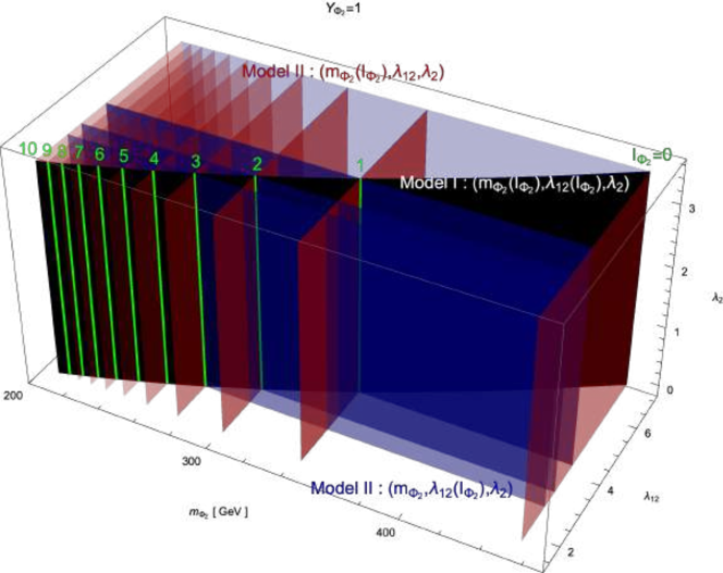
Figure 3: The presentation for a part of the effective models of interest in the parameter space supported by $(m_{\Phi_{2}},\lambda_{12},\lambda_{2})$ with a fixed $Y_{\Phi_{2}}=1$. The black strip is the model I with both $m_{\Phi_{2}}$ and $\lambda_{12}$ determined by $I_{\Phi_{2}}$ labeled in green. For model II, we take two illustrative examples with (1) the same $m_{\Phi_{2}}$ as the model I but a free $\lambda_{12}$ detached from $I_{\Phi_{2}}$ presented as red slices, and (2) the same $\lambda_{12}$ as the model I but a free $m_{\Phi_{2}}$ detached from $I_{\Phi_{2}}$ presented as blue slices.

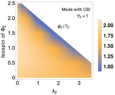
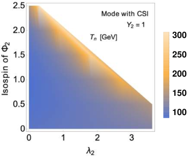
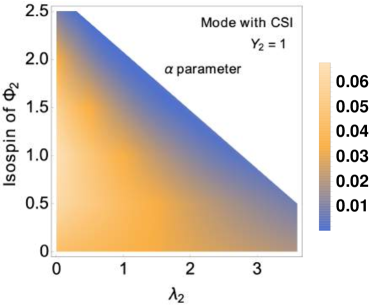
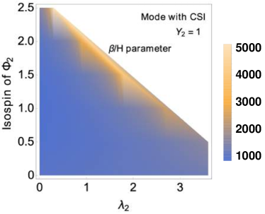
Figure 4: The values of $\phi_{C}/T_{C}$, $T_{n}$, $\alpha$ and $\beta/H$ for the model I with respect to $\lambda_{2}$ coupling and isospin $I_{\Phi_{2}}$ of the additional scalar boson fields.

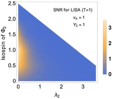
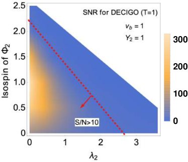
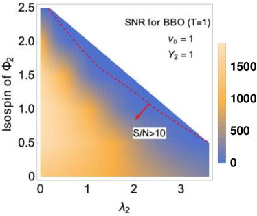
Figure 5: The values of SNR for the model with CSI at LISA, DECIGO and BBO. The experimental period is one year and bubble wall velocity is 1. The red dashed line represents SNR=10.

In this section, we first show the value of $\phi_{C}/T_{C}$ for the model I in the first panel of Fig. 4 to see which part of parameter space could produce detectable GWs. The horizontal axis is the quartic coupling $\lambda_{2}$ and the vertical axis is the isospin $I_{\Phi_{2}}$ of the additional scalar boson fields. It is easy to see that the value of $\phi_{C}/T_{C}$ is large for either small isospin $I_{\Phi_{2}}$ or small $\lambda_{2}$ coupling. This result of $\phi_{C}/T_{C}$ is different from our intuition since the strongly FOPT can be typically realized by adding a large number of additional scalar boson fields into the model, which corresponds to a large isospin $I_{\Phi_{2}}$. In the model with CSI, the number of additional scalar boson fields is related to the Higgs boson mass via Eq. (27). Then, the $\phi_{C}/T_{C}$ without ring diagram contribution is roughly estimated by

$$\frac{\phi_{C}}{T_{C}}=\frac{E}{\lambda_{2}}\propto I_{\Phi_{2}}^{1/4}.$$ (160)

On the other hand, the ring diagram contribution has $I_{\Phi_{2}}^{2}$-dependence in Eq. (3.2), therefore, $\phi_{C}/T_{C}$ becomes small through large ring diagram contributions from large $I_{\Phi_{2}}^{2}$ value.

The PT parameters $T_{n}$, $\alpha$ and $\beta/H$ are shown in the last three panels of Fig. 4, respectively. From these parameters, we can describe the GW spectrum from the FOPT. The SNR for the testability of this model with CSI is shown in Fig. 5 with respect to the future space-borne GW detectors LISA, DECIGO, and BBO. When evaluating the SNR, we simply take the mission duration to be one year and the bubble wall velocity to be one. The red dashed curves in the panels of DECIGO and BBO represent SNR=10. In the parameter regions to the left of the red dashed curves, the SNR is larger than 10, therefore, these parameter regions could be tested at future GW detectors DECIGO and BBO. From these figures, most of parameter regions for the model with CSI could be tested by the DECIGO and BBO missions.

5.2 The model without classical scale invariance

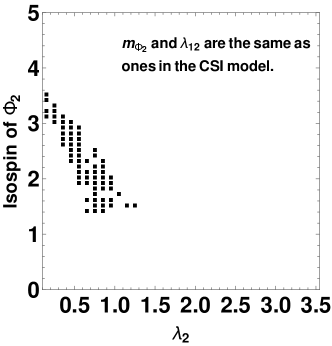
Figure 6: The parameter region can have a stable minimum point along $\varphi_{1}$ and $\varphi_{2}$ axes. At these black points, there is global minimum along $\varphi_{2}$ axis.

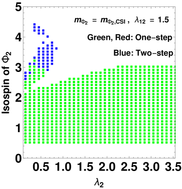
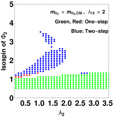
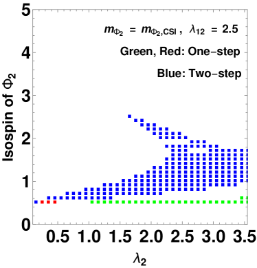
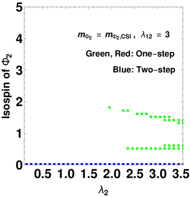
Figure 7: Different PT regions in the parameter space supported by $\lambda_{2}$ and $\Phi_{2}$ for the model II with the same $m_{\Phi_{2}}$ as the model I but allowing for different $\lambda_{12}=1.5,2.0,2.5,3.0$. The blue points represent the two-step PT. The red and green points represent the one-step PT. The detectable GWs at the BBO detection can be generated for the red points. For the rest of regions in this figure, the global minimum point does not appear along $\varphi_{1}$ axis otherwise the potential is unstable.

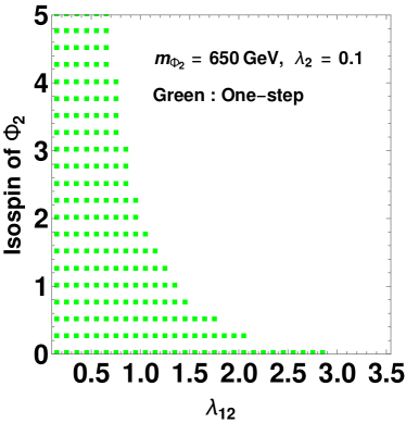
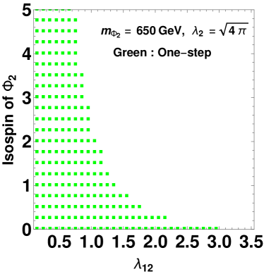
Figure 8: The model parameters for the model II with $\lambda_{2}=0.1,\sqrt{4\pi}$ and $m_{\Phi_{2}}$ = 650 GeV. The horizontal axis in left and right figures is $\lambda_{12}$. Otherwise, the same as Fig. 7.

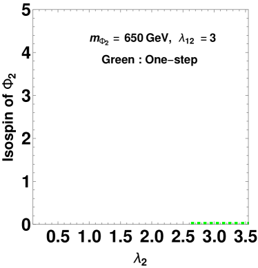
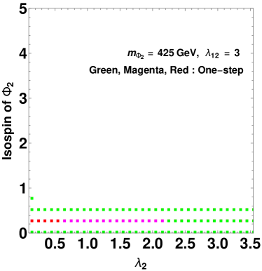
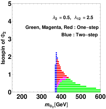
Figure 9: (Upper panels) The model parameters for the model II with $\lambda_{12}=$3 and $m_{\Phi_{2}}$ = 650, 425 GeV in the upper left and upper right panels, respectively. At the red (magenta) marks, the detectable GWs at DECIGO (BBO) can be generated. Otherwise, the same as Fig. 7. (Lower panel) The results in the model with $\lambda_{2}=$0.5 and $\lambda_{12}=$2.5. Horizontal axis is the additional scalar boson mass. The two-step PT occurs at blue marks.

In this section, we show the results for the model II, which admits two more free parameters than the model I, namely, $m_{\Phi_{2}}$ and $\lambda_{12}$. To compare with model I/III with only one-step PT (the additional VEV does not appear in the potential at zero temperature), we will focus on the parameter regions where the same one-step PT for model II as model I/III (green $\to$ red in Fig. 2) can be realized. We also neglect the parameter regions with other paths of PT, for example, two-step PT (namely the path along green $\to$ magenta $\to$ red, where the red is a global minimum). We numerically examine the parameter regions where one-step EWPT can be generated by using following four parameter regions: (i) the same $m_{\Phi_{2}}$ and $\lambda_{12}$ as the model I, (ii) the same $m_{\Phi_{2}}$ as model I, (iii) the same $m_{\Phi_{2}}$ as model III, and (iv) different $m_{\Phi_{2}}$ and $\lambda_{12}$ from other models.

In the parameter region (i), there are the minimum points along $\varphi_{1}$ and $\varphi_{2}$ axes at the black-point region in Fig. 6, but the minimum points along $\varphi_{1}$ and $\varphi_{2}$ axis are local and global minima, respectively. According our numerical results, the two-step PT (green $\to$ red $\to$ magenta) is generated at the black-point region, and the magenta point becomes the true vacuum. In such a case, we cannot explain the fermion mass since the additional scalar field $\Phi_{2}$ does not couple to the fermion fields anymore. Therefore, in the parameter (i) for the model II, we cannot realize a proper PT which can make up the current universe. Although the model I can generate the detectable GW from the one-step EWPT in Fig. 5, the model II cannot realize the correct PT between green and red points in the parameter region (i), which shares the same parameter values as the model I. Therefore, we can distinguish the models with and without CSI by the GW detection.

In the parameter case (ii), model II admits the same $m_{\Phi_{2}}$ given by Eq. (28) as the model I but with $\lambda_{12}=1.5,2.0,2.5,3.0$ decoupled from $I_{\Phi_{2}}$ by Eq. (29) as shown in Fig. 7, respectively. Note that in the case of model I, $m_{\Phi_{2}}$ and $\lambda_{12}$ are related by $m_{\Phi_{2}}^{2}=\lambda_{12}v^{2}/2$, and thus we can get almost the same results for a similar case with the same $\lambda_{12}$ as model I by Eq. (29) but decoupled $m_{\Phi_{2}}$ from $I_{\Phi_{2}}$ by Eq. (28). All colored points in Fig. 7 admit their global minimum along $\varphi_{1}$ (namely the red point in Fig. 2). To show the parameter region where one-step PT along $\varphi_{1}$ axis can be generated, we compare the critical temperatures for the PT along $\varphi_{1}$ and $\varphi_{2}$ axes. From the numerical results, the blue points in Fig. 7 have higher critical temperature for the PTs along $\varphi_{2}$ than the PT for $\varphi_{1}$. On the other hand, the green and red points in Fig. 7 can realize the one-step PT (green $\to$ red in Fig. 2), especially, the red points can realize the strong FOPT along $\varphi_{1}$ axis where the detectable GWs may be generated. At these red points in the model with $\lambda_{12}=2$ and 2.5, the SNR for BBO with mission time $\mathcal{T}$=1 yr and $v_{b}=1$ is larger than 10. Furthermore, the SNR for DECIGO with mission time $\mathcal{T}$=1 yr and $v_{b}=1$ at ($\lambda_{2}$, $I_{\Phi_{2}}$)=(0.25,0.5) is about 10.87, while other red points have their SNR no more than 10 for DECIGO. In short summary, a small $\lambda_{2}$ is necessary for detectable GWs in the model II, which is not necessary for the model I as shown in Fig. 5.

To compare the results between the model II and the model III, we show the results in the parameter region (iii) with heavy $m_{\Phi_{2}}$ as model III. For example, the results for heavy $m_{\Phi_{2}}=650$ GeV with some $\lambda_{2}$ values in the model II are shown in Fig. 8, however, the effects from the additional heavy scalar field decouple. From the additional scalar mass $M_{\Phi_{2}}(\varphi)^{2}\sim-\mu^{2}_{2}+\lambda_{12}\varphi^{2}$ with large $\mu_{2}^{2}$ value, the cubic term of field-dependent mass in the effective potential can be expanded like $(M_{\Phi_{2}}^{2})^{3/2}\sim|\mu^{3}_{2}|+\lambda_{12}\mu_{2}\varphi^{2}+\lambda_{12}^{2}\varphi^{4}/\mu_{2}$, but the cubic $\varphi^{3}$ term does not appear in the potential. On the other hand, the $M_{\Phi_{2}}(\varphi)^{3/2}$ with small $\mu_{2}^{2}$ value can have $\lambda_{12}^{3/2}\varphi^{3}$ as the source of a barrier. Therefore, it is difficult to generate a sizable barrier to realize first-order EWPT in the model II with much heavy additional scalar field. For the large negative $\mu_{2}^{2}$ term, the one-step PT occurs between green and red points in Fig. 2. In this case, $\lambda_{2}$, which is the coefficient of $\Phi_{2}^{4}$, does not much affect the EWPT, and the results are not very different between two figures of Fig. 8.

Upper panels in Fig. 9 represent the results in the model with $\lambda_{12}$=3 and $m_{\Phi_{2}}=650$ and 425 GeV, which correspond to the parameter regions (iii) and (iv), respectively. With these parameters, the mass parameter $\mu_{2}$ becomes small (non-decoupling) and the detectable GW spectrum can be generated. Especially, in the model with $m_{\Phi_{2}}=$ 425 GeV, the red (magenta) marks can be described in the upper right figure, and the SNR for DECIGO (BBO) is larger than 10. The lower panel in Fig. 9 represents the results with respect to $I_{\Phi_{2}}$ and $m_{\Phi_{2}}$, which are related to parameter region (iv) in the model with benchmark parameters $\lambda_{2}=$0.5 and $\lambda_{12}=$2.5. The blue marks in this model can realize two-step PT. In short summary, the detectable GWs, which are represented by red and magenta marks, can be produced in the massive model with small isospin of $\Phi_{2}$ and small $\lambda_{2}$ value. However, for the model II, such parameter regions with detectable GWs are not the same as those in model I and model III. Therefore we may distinguish the three types of models by the GW observations.

5.3 The model with dimension-six operator from $\Phi_{2}$

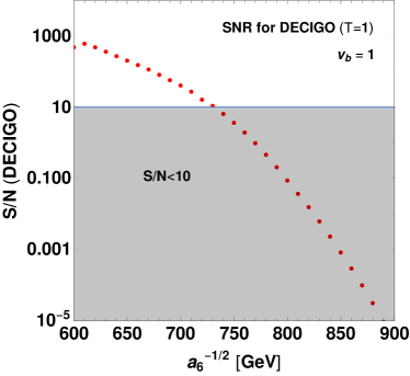
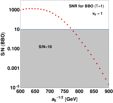
Figure 10: The SNR value from the model with a higher dimensional operator for DECIGO and BBO with mission year $\mathcal{T}=1$ yr and $v_{b}=1$.

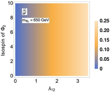
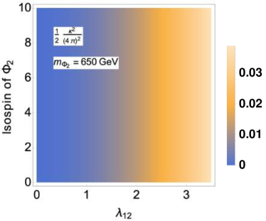
Figure 11: The values of parameters $U/m_{\Phi_{2}}^{2}$ and $\frac{\kappa^{2}}{32\pi^{2}}$ for a valid EFT expansion in the model with a higher dimensional operator with respect to $I_{\Phi_{2}}$ and $\lambda_{12}$ and fixed $m_{\Phi_{2}}=650$ GeV. For the presented parameter regions, the conditions $\frac{U}{M^{2}}\ll 1$ and $\frac{c_{i}\kappa^{2}}{16\pi^{2}}\ll 1$ for a valid EFT expansion can be satisfied.

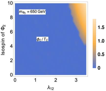
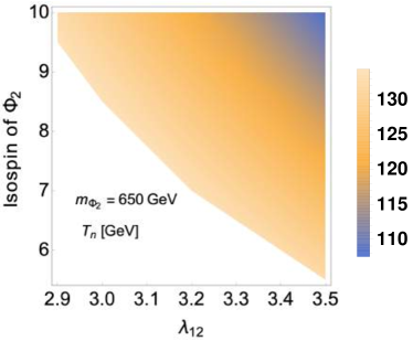
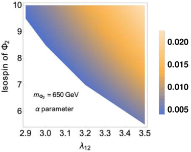
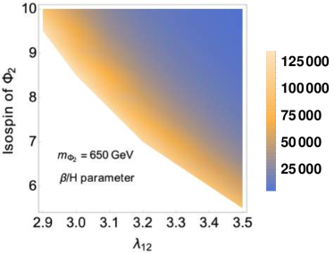
Figure 12: The value of $\phi_{C}/T_{C}$, $T_{n}$, $\alpha$ and $\beta/H$ in the EFT model with $m_{\Phi_{2}}=650$ GeV. Otherwise, the same as Fig. 11.

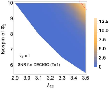
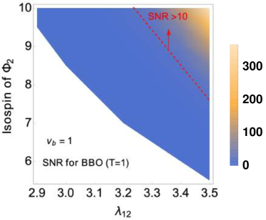
Figure 13: The values of SNR in the EFT model with $m_{\Phi_{2}}=650$ GeV at DECIGO and BBO. The ratio of SNR is larger than 10 in the parameter region to right of the red dashed lines.

In this section, we discuss the testability for the model III. At first, the parameter region of $a_{6}$ is shown in Fig. 10 for detectable GWs at DECIGO and BBO with mission duration $\mathcal{T}=1$ yr and $v_{b}=1$. In the dark regions, the SNR is smaller than 10, hence we require for a large $a_{6}$ value. Recall that with Eq. (19), $a_{6}=(1+2I_{\Phi_{2}})\frac{1}{(4\pi)^{2}m_{\Phi_{2}}^{2}}\left(\frac{\lambda_{12}^{3}}{8}+\frac{\lambda_{12}^{2}\lambda_{1}}{6}\right)$, a large $a_{6}$ value generally prefers a large isospin $I_{\Phi_{2}}$, namely a large number of the additional scalar boson fields. This circumvents the difficulty mentioned at the end of Section 2, and we should further check the balance between $U/M^{2}$ and $\frac{c_{i}\kappa^{2}}{16\pi^{2}}$ for a valid EFT expansion. In the left and right panels of Fig. 11, the values of $U/m_{\Phi_{2}}^{2}$ and $\frac{\kappa^{2}}{32\pi^{2}}$ are shown for given $I_{\Phi_{2}}$ and $\lambda_{12}$, respectively. For the presented parameter space, the conditions $\frac{U}{M^{2}}\ll 1$ and $\frac{c_{i}\kappa^{2}}{16\pi^{2}}\ll 1$ for a valid EFT expansion are satisfied.

The values of $\phi_{C}/T_{C}$, $T_{n}$, $\alpha$ and $\beta/H$ are then shown in Fig. 12 and the corresponding SNR at DECIGO and BBO are shown in Fig. 13, where the parameter regions to the right of red dashed lines have their SNR larger than 10. However, SNR is less than $10^{-5}$ for LISA, hence LISA may be difficult to test the parameter region of the model III. For detectable GWs from the model III, we require a large number of additional scalar fields (namely a large isospin $I_{\Phi_{2}}$) and large coupling $\lambda_{12}$, which can be distinguished from models I and II by detectable GWs in the parameter regions of small isospin $I_{\Phi_{2}}$. In particular, the model I cannot take the heavy scalar field with $m_{\Phi_{2}}=650$ GeV since the additional scalar mass should be less than 543 GeV from Eq. (28) Hashino:2015nxa . Therefore, we may distinguish the model III from model I and model II by constraining the isospin of additional scalar fields with the GWs background observed at future GW detectors.

6 Conclusions and discussions

The predictions for the GW background vary sensitively among different concrete models but also share a large degeneracy in the model buildings. From that, in this time, we take into account an EFT treatment for three BSM models based on different patterns of the EWSB: (I) classical scale invariance, (II) generic scalar extension, and (III) higher dimensional operators. In these EFTs, the EWSB can be realized by (I) radiative symmetry breaking, (II) Higgs mechanism, and (III) EFT description of EWSB, respectively.

These three models can realize the strongly first-order EWPT and can produce the detectable GW spectrum by the effects summarized in Tab. 2. Here, $C_{n}$ are the effective couplings of the order parameter operators $\phi^{n}$ in the effective potential. The dominant contributions of $\lambda_{2}$ and $I_{\Phi_{2}}$ in models (I) and (II) show up through the ring diagram effects as shown in Eqs (31), (42), (3.2) and (63). Thus, a small $\lambda_{2}$ and a small $I_{\Phi_{2}}$ are required to produce the detectable GW spectrum. The differences between models (I) and (II) are the $C_{2}$ and $C_{4}$ terms and the number of free parameters in the model. In the model (II), these terms have the tree-level contribution, and thus we need to tune model parameters to have a sizable $C_{3}$ comparable with these $C_{2}$ and $C_{4}$ terms. Unlike the model (I), we can use the $\lambda_{12}$ parameter to realize such a situation and could generate the first-order EWPT as shown in Fig. 7. On the other hand, the $\lambda_{2}$ in model (III) does not contribute to the effective potential after integrating out the $\Phi_{2}$ scalar field, and the high dimensional operator $a_{6}^{-1/2}$ in Fig. 10 is inversely proportional to $\lambda_{12}$ and $I_{\Phi_{2}}$ as shown in Eq. (19). Therefore, a small $a_{6}^{-1/2}$ can be realized by a large $\lambda_{12}$ and a large $I_{\Phi_{2}}$.

Model	$C_{2}\phi^{2}$	$C_{3}\phi^{3}$	$C_{4}\phi^{4}$	$C_{6}\phi^{6}$	GW features
I	Loop	Loop	Loop	None	Small $\lambda_{2}$ and small $I_{\Phi_{2}}$
II	Tree	Loop	Tree	None	Small $\lambda_{2}$ and small $I_{\Phi_{2}}$
III	Tree	Loop	Tree	Tree	Large $\lambda_{12}$ and large $I_{\Phi_{2}}$

Table 2: The potential forms in the three types of the models where the EWSB can be realized by (I) radiative symmetry breaking, (II) Higgs mechanism and (III) EFT description of EWSB, respectively. The last column shows the source of detectable GW spectrum in these models. Otherwise, the same as Tab. 1.

These three types of models might be distinguished by investigating the detectable GWs in the parameter regions with overlapping parameters: (1) Model I and model II might be distinguished by the detection of GWs in the parameter regions as shown in Figs. 5 and 6. When taking the same $m_{\Phi_{2}}$ and $\lambda_{12}$ as model I by Eqs. (28) and (29), model II cannot generate the correct one-step PT where the red point in Fig. 2 is the local minimum. However, when just taking the same $m_{\Phi_{2}}$ as model I by Eq. (28) but decoupling $\lambda_{12}$ from $I_{\Phi_{2}}$ by Eq. (29), model II could produce detactable GWs in the parameter regions of small $\lambda_{2}$ and small $I_{\Phi_{2}}$, which is partially overlapping with model I with detectable GWs. In this case, although we cannot fully distinguish models I and II by the GW detections alone, we may use other observations, such as $hhh$ coupling, to do that Hashino:2016rvx . (2) Model II and model III can be distinguished by the detection of GWs in the parameter regions as shown in Figs. 8 and 13 since detectable GWs are produced for model II in the parameter regions of small $\lambda_{2}$ and small $I_{\Phi_{2}}$, while model III favors a large $I_{\Phi_{2}}$ to generate detectable GWs. (3) Similarly, model I could also be distinguished from model III by detectable GWs in the parameter regions of small $I_{\Phi_{2}}$ (model I) and large $I_{\Phi_{2}}$ (model III). Furthermore, the additional scalar mass should be less than 543 GeV in the model I, different from the case of model III with a heavy scalar field.

Therefore, we may distinguish these three effective model descriptions of EWPT by future GW detections in space. Nevertheless, our PT analysis for the effective model descriptions is preliminary in surveying part of the parameter space, and it only depicts those scalar extensions (with $Z_{2}$ symmetry) of fundamental Higgs models Corbett:2017ieo ; Li:2020gnx ; Li:2020xlh and Coleman-Weinberg Higgs models Hill:2014mqa ; Helmboldt:2016mpi ; Hashino:2015nxa , but by no means covers all the effective models of EWPT. We will investigate the PT dynamics in a more general classifications of EWSB Agrawal:2019bpm in the ever-enlarging parameter space in future works.

Appendix A Stationary condition and CP-even boson masses in the model without CSI

We use the stationary condition at ($\varphi_{1}$, $\varphi_{2}$) = ($v$, 0) and the second derivatives of the potential with one-loop effects,

$$\left.\frac{\partial V_{eff}}{\partial\left\langle\Phi_{1}\right\rangle}\right|_{\left\langle\Phi_{1}\right\rangle=v,\left\langle\Phi_{2}\right\rangle=0}=0,\quad\left.\frac{\partial^{2}V_{eff}}{\partial\left\langle\Phi_{1}\right\rangle^{2}}\right|_{\left\langle\Phi_{1}\right\rangle=v,\left\langle\Phi_{2}\right\rangle=0}=m_{h}^{2},$$ (161)

where we take $Q=v=246$ GeV. With tadpole condition ${\cal M}_{\Phi_{2}\Phi_{2}}^{2}>{\cal M}_{\Phi_{1}\Phi_{1}}^{2}$, one arrives at

$$\left.\frac{\partial V_{\rm eff}}{\partial\left\langle\Phi_{1}\right\rangle}\right|_{\left\langle\Phi_{1}\right\rangle=v,\left\langle\Phi_{2}\right\rangle=0} =-\mu_{1}^{2}+\lambda_{1}v^{2}+\frac{1}{16\pi^{2}}\Bigg{[}\frac{6\lambda_{1}+\lambda_{12}}{4}f_{+}(m_{\Phi_{1,r}}^{2},m_{\Phi_{2,r}}^{2})+\frac{1}{4}(6\lambda_{1}-\lambda_{12})f_{-}(m_{\Phi_{1,r}}^{2},m_{\Phi_{2,r}}^{2})$$

$$\quad+(2(2I_{\Phi_{2}}-1)-1)\frac{\lambda_{12}m_{N_{2,r}}^{2}}{2}\left(\ln\frac{m_{N_{2,r}}^{2}}{Q^{2}}-1\right)+\frac{6m_{W}^{4}}{v^{2}}\left(\ln\frac{m_{W}^{2}}{Q^{2}}-\frac{1}{3}\right)$$

$$\quad+\frac{3m_{Z}^{4}}{v^{2}}\left(\ln\frac{m_{Z}^{2}}{Q^{2}}-\frac{1}{3}\right)-\frac{12m_{t}^{4}}{v^{2}}\left(\ln\frac{m_{t}^{2}}{Q^{2}}-1\right)\Bigg{]}=0,$$ (162)

where

$$f_{\pm}(m_{i}^{2},m_{j}^{2}) =m_{i}^{2}\left(\ln\frac{m_{i}^{2}}{Q^{2}}-1\right)\pm m_{j}^{2}\left(\ln\frac{m_{j}^{2}}{Q^{2}}-1\right),$$ (163)

$$\Delta m_{\Phi}^{2} =m_{\Phi_{2}}^{2}-m_{\Phi_{1}}^{2}=\sqrt{\left({\cal M}_{\Phi_{1}\Phi_{1}}^{2}-{\cal M}_{\Phi_{2}\Phi_{2}}^{2}\right)^{2}+4{\cal M}_{\Phi_{1}\Phi_{2}}^{4}},$$ (164)

$$\mathcal{M}_{neutral\,\,Higgs}^{2} =\left(\begin{array}[]{ccc}{\cal M}_{\Phi_{1}\Phi_{1}}^{2}&{\cal M}_{\Phi_{1}\Phi_{2}}^{2}\\ {\cal M}_{\Phi_{2}\Phi_{1}}^{2}&{\cal M}_{\Phi_{2}\Phi_{2}}^{2}\end{array}\right)$$ (167)

and the masses in the tadpole conditions of red point case are

$$m_{\Phi_{1,r}}^{2} =-\mu_{1}^{2}+3\lambda_{1}v^{2},\quad m_{\Phi_{2,r}}^{2}=-\mu_{2}^{2}+\lambda_{12}v^{2}/2,\quad m_{N_{1,r}}^{2}=-\mu_{1}^{2}+\lambda_{1}v^{2},\quad m_{N_{2,r}}^{2}=-\mu_{2}^{2}+\lambda_{12}v^{2}/2,$$ (168)

with $m_{\Phi_{2}}^{2}>m_{h}^{2}$. In order to replace two of the input parameters in the potential in terms of the Higgs boson mass $m_{h}$ and additional neutral CP-even boson mass $m_{\Phi_{2}}$ , we use

$$\left.\frac{\partial^{2}V_{\rm eff}}{\partial\left\langle\Phi_{1}\right\rangle^{2}}\right|_{\left\langle\Phi_{1}\right\rangle=v,\left\langle\Phi_{2}\right\rangle=0} =2\lambda_{1}v^{2}+\frac{v^{2}}{32\pi^{2}}\Bigg{[}A^{r}_{2}\ln\frac{m_{\Phi_{2}}^{2}m_{h}^{2}}{Q^{4}}-A^{r}_{3}\ln\frac{m_{h}^{2}}{m_{\Phi_{2}}^{2}}+4\lambda_{12}^{2}(2(2I_{\Phi_{2}}-1)-1)\ln\frac{m_{N_{2,r}}^{2}}{Q^{2}}$$

$$\quad+12\frac{m_{Z}^{4}}{v^{4}}\left(\ln\frac{m_{Z}^{2}}{Q^{2}}+\frac{2}{3}\right)+24\frac{m_{W}^{4}}{v^{4}}\left(\ln\frac{m_{W}^{2}}{Q^{2}}+\frac{2}{3}\right)-48\frac{m_{t}^{4}}{v^{4}}\ln\frac{m_{t}^{2}}{Q^{2}}\Bigg{]}\equiv m_{h}^{2}$$ (169)

$$\left.\frac{\partial^{2}V_{\rm eff}}{\partial\left\langle\Phi_{2}\right\rangle^{2}}\right|_{\left\langle\Phi_{1}\right\rangle=v,\left\langle\Phi_{2}\right\rangle=0} =-\mu_{2}^{2}+\lambda_{12}v^{2}+\frac{1}{64\pi^{2}}\Bigg{[}B_{1}f_{-}(m_{\Phi_{2}}^{2},m_{h}^{2})+B_{2}f_{+}(m_{\Phi_{2}}^{2},m_{h}^{2})$$

$$\quad+4(2(2I_{\Phi_{2}}-1)-1)\lambda_{2}m_{N_{2,r}}^{2}\left(\ln\frac{m_{N_{2,r}}^{2}}{Q^{2}}-1\right)+12\frac{m_{Z}^{4}Y_{\Phi_{2}}^{2}}{v^{2}}\left(\ln\frac{m_{Z}^{2}}{Q^{2}}-\frac{1}{3}\right)$$

$$\quad+24\frac{m_{W}^{4}I_{W}^{2}}{v^{2}}\left(\ln\frac{m_{W}^{2}}{Q^{2}}-\frac{1}{3}\right)\Bigg{]}\equiv m_{\Phi_{2}}^{2},$$ (170)

where

$$A^{r}_{2} =\frac{1}{4}\left((6\lambda_{1}+\lambda_{12})^{2}+(6\lambda_{1}-\lambda_{12})^{2}\right),\quad A^{r}_{3}=-\frac{36\lambda_{1}^{2}-\lambda_{12}^{2}}{2}$$ (171)

$$B_{1} =\frac{2}{\Delta m^{2}}\left[\left(-6\lambda_{2}+\lambda_{12}\right)\left({\cal M}_{\Phi_{1}\Phi_{1}}^{2}-{\cal M}_{\Phi_{2}\Phi_{2}}^{2}\right)+4\lambda_{12}^{2}v^{2}\right]$$ (172)

$$B_{2} =6\lambda_{2}+\lambda_{12}.$$ (173)

By using Eqs. (A), (A) and (A), we can replace the model parameters:

$$(\mu_{1}^{2},\mu_{2}^{2},\lambda_{1},\lambda_{2},\lambda_{12})\to(v,m_{\Phi_{2}}^{2},m_{h},\lambda_{2},\lambda_{12}).$$ (174)

References

- (1) Particle Data Group collaboration, P. Zyla et al., Review of Particle Physics, PTEP 2020 (2020) 083C01.
- (2) A. Mazumdar and G. White, Review of cosmic phase transitions: their significance and experimental signatures, Rept. Prog. Phys. 82 (2019) 076901, [1811.01948].
- (3) M. B. Hindmarsh, M. Lüben, J. Lumma and M. Pauly, Phase transitions in the early universe, 2008.09136.
- (4) C. Caprini et al., Science with the space-based interferometer eLISA. II: Gravitational waves from cosmological phase transitions, JCAP 1604 (2016) 001, [1512.06239].
- (5) C. Caprini et al., Detecting gravitational waves from cosmological phase transitions with LISA: an update, JCAP 2003 (2020) 024, [1910.13125].
- (6) LISA collaboration, P. Amaro-Seoane et al., Laser Interferometer Space Antenna, 1702.00786.
- (7) P. Binetruy, A. Bohe, C. Caprini and J.-F. Dufaux, Cosmological Backgrounds of Gravitational Waves and eLISA/NGO: Phase Transitions, Cosmic Strings and Other Sources, JCAP 1206 (2012) 027, [1201.0983].
- (8) P. Amaro-Seoane et al., Low-frequency gravitational-wave science with eLISA/NGO, Class. Quant. Grav. 29 (2012) 124016, [1202.0839].
- (9) P. Amaro-Seoane et al., eLISA/NGO: Astrophysics and cosmology in the gravitational-wave millihertz regime, GW Notes 6 (2013) 4–110, [1201.3621].
- (10) D. J. Weir, Gravitational waves from a first order electroweak phase transition: a brief review, Phil. Trans. Roy. Soc. Lond. A376 (2018) 20170126, [1705.01783].
- (11) D. G. Figueroa, E. Megias, G. Nardini, M. Pieroni, M. Quiros, A. Ricciardone et al., LISA as a probe for particle physics: electroweak scale tests in synergy with ground-based experiments, PoS GRASS2018 (2018) 036, [1806.06463].
- (12) M. Fitz Axen, S. Banagiri, A. Matas, C. Caprini and V. Mandic, Multiwavelength observations of cosmological phase transitions using LISA and Cosmic Explorer, Phys. Rev. D98 (2018) 103508, [1806.02500].
- (13) R.-G. Cai, Z. Cao, Z.-K. Guo, S.-J. Wang and T. Yang, The Gravitational-Wave Physics, Natl. Sci. Rev. 4 (2017) 687–706, [1703.00187].
- (14) L. Bian et al., The Gravitational-wave physics II: Progress, Sci. China Phys. Mech. Astron. 64 (2021) 120401, [2106.10235].
- (15) K. Kajantie, M. Laine, K. Rummukainen and M. E. Shaposhnikov, Is there a hot electroweak phase transition at m(H) larger or equal to m(W)?, Phys. Rev. Lett. 77 (1996) 2887–2890, [hep-ph/9605288].
- (16) X.-m. Zhang, Operators analysis for Higgs potential and cosmological bound on Higgs mass, Phys. Rev. D47 (1993) 3065–3067, [hep-ph/9301277].
- (17) D. Bodeker, L. Fromme, S. J. Huber and M. Seniuch, The Baryon asymmetry in the standard model with a low cut-off, JHEP 02 (2005) 026, [hep-ph/0412366].
- (18) C. Grojean, G. Servant and J. D. Wells, First-order electroweak phase transition in the standard model with a low cutoff, Phys. Rev. D71 (2005) 036001, [hep-ph/0407019].
- (19) C. Delaunay, C. Grojean and J. D. Wells, Dynamics of Non-renormalizable Electroweak Symmetry Breaking, JHEP 04 (2008) 029, [0711.2511].
- (20) S. J. Huber and T. Konstandin, Production of gravitational waves in the nMSSM, JCAP 0805 (2008) 017, [0709.2091].
- (21) S. J. Huber and M. Sopena, An efficient approach to electroweak bubble velocities, 1302.1044.
- (22) T. Konstandin, G. Nardini and I. Rues, From Boltzmann equations to steady wall velocities, JCAP 1409 (2014) 028, [1407.3132].
- (23) P. H. Damgaard, A. Haarr, D. O’Connell and A. Tranberg, Effective Field Theory and Electroweak Baryogenesis in the Singlet-Extended Standard Model, JHEP 02 (2016) 107, [1512.01963].
- (24) L. Leitao and A. Megevand, Gravitational waves from a very strong electroweak phase transition, JCAP 1605 (2016) 037, [1512.08962].
- (25) C. P. D. Harman and S. J. Huber, Does zero temperature decide on the nature of the electroweak phase transition?, JHEP 06 (2016) 005, [1512.05611].
- (26) F. P. Huang, Y. Wan, D.-G. Wang, Y.-F. Cai and X. Zhang, Hearing the echoes of electroweak baryogenesis with gravitational wave detectors, Phys. Rev. D94 (2016) 041702, [1601.01640].
- (27) C. Balazs, G. White and J. Yue, Effective field theory, electric dipole moments and electroweak baryogenesis, JHEP 03 (2017) 030, [1612.01270].
- (28) J. de Vries, M. Postma, J. van de Vis and G. White, Electroweak Baryogenesis and the Standard Model Effective Field Theory, JHEP 01 (2018) 089, [1710.04061].
- (29) R.-G. Cai, M. Sasaki and S.-J. Wang, The gravitational waves from the first-order phase transition with a dimension-six operator, JCAP 1708 (2017) 004, [1707.03001].
- (30) M. Chala, C. Krause and G. Nardini, Signals of the electroweak phase transition at colliders and gravitational wave observatories, JHEP 07 (2018) 062, [1802.02168].
- (31) G. C. Dorsch, S. J. Huber and T. Konstandin, Bubble wall velocities in the Standard Model and beyond, JCAP 1812 (2018) 034, [1809.04907].
- (32) J. De Vries, M. Postma and J. van de Vis, The role of leptons in electroweak baryogenesis, JHEP 04 (2019) 024, [1811.11104].
- (33) S. A. R. Ellis, S. Ipek and G. White, Electroweak Baryogenesis from Temperature-Varying Couplings, JHEP 08 (2019) 002, [1905.11994].
- (34) M. Chala, V. V. Khoze, M. Spannowsky and P. Waite, Mapping the shape of the scalar potential with gravitational waves, Int. J. Mod. Phys. A34 (2019) 1950223, [1905.00911].
- (35) R. Zhou, L. Bian and H.-K. Guo, Connecting the electroweak sphaleron with gravitational waves, Phys. Rev. D101 (2020) 091903, [1910.00234].
- (36) V. Q. Phong, P. H. Khiem, N. P. D. Loc and H. N. Long, Sphaleron in the first-order electroweak phase transition with the dimension-six Higgs field operator, Phys. Rev. D101 (2020) 116010, [2003.09625].
- (37) S. Kanemura and M. Tanaka, Higgs boson coupling as a probe of the sphaleron property, Phys. Lett. B 809 (2020) 135711, [2005.05250].
- (38) K. Hashino, S. Kanemura and T. Takahashi, Primordial black holes as a probe of strongly first-order electroweak phase transition, 2111.13099.
- (39) S. Kanemura and R. Nagai, A new Higgs effective field theory and the new no-lose theorem, 2111.12585.
- (40) S. Profumo, M. J. Ramsey-Musolf and G. Shaughnessy, Singlet Higgs phenomenology and the electroweak phase transition, JHEP 08 (2007) 010, [0705.2425].
- (41) J. R. Espinosa, T. Konstandin and F. Riva, Strong Electroweak Phase Transitions in the Standard Model with a Singlet, Nucl. Phys. B854 (2012) 592–630, [1107.5441].
- (42) S. Profumo, M. J. Ramsey-Musolf, C. L. Wainwright and P. Winslow, Singlet-catalyzed electroweak phase transitions and precision Higgs boson studies, Phys. Rev. D91 (2015) 035018, [1407.5342].
- (43) R. Jinno, K. Nakayama and M. Takimoto, Gravitational waves from the first order phase transition of the Higgs field at high energy scales, Phys. Rev. D93 (2016) 045024, [1510.02697].
- (44) P. Huang, A. J. Long and L.-T. Wang, Probing the Electroweak Phase Transition with Higgs Factories and Gravitational Waves, Phys. Rev. D94 (2016) 075008, [1608.06619].
- (45) C. Balazs, A. Fowlie, A. Mazumdar and G. White, Gravitational waves at aLIGO and vacuum stability with a scalar singlet extension of the Standard Model, Phys. Rev. D95 (2017) 043505, [1611.01617].
- (46) D. Curtin, P. Meade and H. Ramani, Thermal Resummation and Phase Transitions, Eur. Phys. J. C78 (2018) 787, [1612.00466].
- (47) K. Hashino, M. Kakizaki, S. Kanemura, P. Ko and T. Matsui, Gravitational waves and Higgs boson couplings for exploring first order phase transition in the model with a singlet scalar field, Phys. Lett. B766 (2017) 49–54, [1609.00297].
- (48) V. Vaskonen, Electroweak baryogenesis and gravitational waves from a real scalar singlet, Phys. Rev. D95 (2017) 123515, [1611.02073].
- (49) G. Kurup and M. Perelstein, Dynamics of Electroweak Phase Transition In Singlet-Scalar Extension of the Standard Model, Phys. Rev. D96 (2017) 015036, [1704.03381].
- (50) A. Beniwal, M. Lewicki, J. D. Wells, M. White and A. G. Williams, Gravitational wave, collider and dark matter signals from a scalar singlet electroweak baryogenesis, JHEP 08 (2017) 108, [1702.06124].
- (51) Z. Kang, P. Ko and T. Matsui, Strong first order EWPT & strong gravitational waves in Z3-symmetric singlet scalar extension, JHEP 02 (2018) 115, [1706.09721].
- (52) C.-Y. Chen, J. Kozaczuk and I. M. Lewis, Non-resonant Collider Signatures of a Singlet-Driven Electroweak Phase Transition, JHEP 08 (2017) 096, [1704.05844].
- (53) W. Chao, H.-K. Guo and J. Shu, Gravitational Wave Signals of Electroweak Phase Transition Triggered by Dark Matter, JCAP 1709 (2017) 009, [1702.02698].
- (54) A. Beniwal, M. Lewicki, M. White and A. G. Williams, Gravitational waves and electroweak baryogenesis in a global study of the extended scalar singlet model, JHEP 02 (2019) 183, [1810.02380].
- (55) V. R. Shajiee and A. Tofighi, Electroweak Phase Transition, Gravitational Waves and Dark Matter in Two Scalar Singlet Extension of The Standard Model, Eur. Phys. J. C79 (2019) 360, [1811.09807].
- (56) A. Alves, T. Ghosh, H.-K. Guo, K. Sinha and D. Vagie, Collider and Gravitational Wave Complementarity in Exploring the Singlet Extension of the Standard Model, JHEP 04 (2019) 052, [1812.09333].
- (57) B. Grzadkowski and D. Huang, Spontaneous -Violating Electroweak Baryogenesis and Dark Matter from a Complex Singlet Scalar, JHEP 08 (2018) 135, [1807.06987].
- (58) K. Hashino, R. Jinno, M. Kakizaki, S. Kanemura, T. Takahashi and M. Takimoto, Selecting models of first-order phase transitions using the synergy between collider and gravitational-wave experiments, Phys. Rev. D99 (2019) 075011, [1809.04994].
- (59) A. Ahriche, K. Hashino, S. Kanemura and S. Nasri, Gravitational Waves from Phase Transitions in Models with Charged Singlets, Phys. Lett. B789 (2019) 119–126, [1809.09883].
- (60) B. Imtiaz, Y.-F. Cai and Y. Wan, Two-field cosmological phase transitions and gravitational waves in the singlet Majoron model, Eur. Phys. J. C79 (2019) 25, [1804.05835].
- (61) N. Chen, T. Li, Y. Wu and L. Bian, Complementarity of the future colliders and gravitational waves in the probe of complex singlet extension to the standard model, Phys. Rev. D101 (2020) 075047, [1911.05579].
- (62) A. Alves, D. Gonçalves, T. Ghosh, H.-K. Guo and K. Sinha, Di-Higgs Production in the Channel and Gravitational Wave Complementarity, JHEP 03 (2020) 053, [1909.05268].
- (63) K. Kannike, K. Loos and M. Raidal, Gravitational wave signals of pseudo-Goldstone dark matter in the complex singlet model, Phys. Rev. D101 (2020) 035001, [1907.13136].
- (64) C.-W. Chiang and B.-Q. Lu, First-order electroweak phase transition in a complex singlet model with symmetry, JHEP 07 (2020) 082, [1912.12634].
- (65) J. Kozaczuk, M. J. Ramsey-Musolf and J. Shelton, Exotic Higgs boson decays and the electroweak phase transition, Phys. Rev. D101 (2020) 115035, [1911.10210].
- (66) M. Carena, Z. Liu and Y. Wang, Electroweak phase transition with spontaneous Z2-breaking, JHEP 08 (2020) 107, [1911.10206].
- (67) A. Alves, D. Gonçalves, T. Ghosh, H.-K. Guo and K. Sinha, Di-Higgs Blind Spots in Gravitational Wave Signals, 2007.15654.
- (68) P. Di Bari, D. Marfatia and Y.-L. Zhou, Gravitational waves from neutrino mass and dark matter genesis, Phys. Rev. D102 (2020) 095017, [2001.07637].
- (69) M. Pandey and A. Paul, Gravitational Wave Emissions from First Order Phase Transitions with Two Component FIMP Dark Matter, 2003.08828.
- (70) T. Alanne, N. Benincasa, M. Heikinheimo, K. Kannike, V. Keus, N. Koivunen et al., Pseudo-Goldstone dark matter: gravitational waves and direct-detection blind spots, JHEP 10 (2020) 080, [2008.09605].
- (71) A. Paul, U. Mukhopadhyay and D. Majumdar, Gravitational Wave Signatures from Domain Wall and Strong First-Order Phase Transitions in a Two Complex Scalar extension of the Standard Model, 2010.03439.
- (72) K.-P. Xie, Lepton-mediated electroweak baryogenesis, gravitational waves and the final state at the collider, 2011.04821.
- (73) S. Kanemura and M. Tanaka, Strongly first-order electroweak phase transition by relatively heavy additional Higgs bosons, 2201.04791.
- (74) P. Huet and A. E. Nelson, CP violation and electroweak baryogenesis in extensions of the standard model, Phys. Lett. B355 (1995) 229–235, [hep-ph/9504427].
- (75) J. M. Cline and P.-A. Lemieux, Electroweak phase transition in two Higgs doublet models, Phys. Rev. D55 (1997) 3873–3881, [hep-ph/9609240].
- (76) L. Fromme, S. J. Huber and M. Seniuch, Baryogenesis in the two-Higgs doublet model, JHEP 11 (2006) 038, [hep-ph/0605242].
- (77) J. M. Cline, K. Kainulainen and M. Trott, Electroweak Baryogenesis in Two Higgs Doublet Models and B meson anomalies, JHEP 11 (2011) 089, [1107.3559].
- (78) G. C. Dorsch, S. J. Huber and J. M. No, A strong electroweak phase transition in the 2HDM after LHC8, JHEP 10 (2013) 029, [1305.6610].
- (79) G. C. Dorsch, S. J. Huber, K. Mimasu and J. M. No, Echoes of the Electroweak Phase Transition: Discovering a second Higgs doublet through , Phys. Rev. Lett. 113 (2014) 211802, [1405.5537].
- (80) M. Kakizaki, S. Kanemura and T. Matsui, Gravitational waves as a probe of extended scalar sectors with the first order electroweak phase transition, Phys. Rev. D92 (2015) 115007, [1509.08394].
- (81) G. C. Dorsch, S. J. Huber, T. Konstandin and J. M. No, A Second Higgs Doublet in the Early Universe: Baryogenesis and Gravitational Waves, JCAP 1705 (2017) 052, [1611.05874].
- (82) P. Basler, M. Krause, M. Muhlleitner, J. Wittbrodt and A. Wlotzka, Strong First Order Electroweak Phase Transition in the CP-Conserving 2HDM Revisited, JHEP 02 (2017) 121, [1612.04086].
- (83) J. Bernon, L. Bian and Y. Jiang, A new insight into the phase transition in the early Universe with two Higgs doublets, JHEP 05 (2018) 151, [1712.08430].
- (84) G. C. Dorsch, S. J. Huber, K. Mimasu and J. M. No, The Higgs Vacuum Uplifted: Revisiting the Electroweak Phase Transition with a Second Higgs Doublet, JHEP 12 (2017) 086, [1705.09186].
- (85) F. P. Huang and J.-H. Yu, Exploring inert dark matter blind spots with gravitational wave signatures, Phys. Rev. D98 (2018) 095022, [1704.04201].
- (86) P. Basler, M. Mühlleitner and J. Wittbrodt, The CP-Violating 2HDM in Light of a Strong First Order Electroweak Phase Transition and Implications for Higgs Pair Production, JHEP 03 (2018) 061, [1711.04097].
- (87) B. Barman, A. Dutta Banik and A. Paul, Singlet-doublet fermionic dark matter and gravitational waves in a two-Higgs-doublet extension of the Standard Model, Phys. Rev. D101 (2020) 055028, [1912.12899].
- (88) X. Wang, F. P. Huang and X. Zhang, Gravitational wave and collider signals in complex two-Higgs doublet model with dynamical CP-violation at finite temperature, Phys. Rev. D101 (2020) 015015, [1909.02978].
- (89) R. Zhou and L. Bian, Baryon asymmetry and detectable Gravitational Waves from Electroweak phase transition, 2001.01237.
- (90) H. H. Patel and M. J. Ramsey-Musolf, Stepping Into Electroweak Symmetry Breaking: Phase Transitions and Higgs Phenomenology, Phys. Rev. D88 (2013) 035013, [1212.5652].
- (91) S. Inoue, G. Ovanesyan and M. J. Ramsey-Musolf, Two-Step Electroweak Baryogenesis, Phys. Rev. D93 (2016) 015013, [1508.05404].
- (92) N. Blinov, J. Kozaczuk, D. E. Morrissey and C. Tamarit, Electroweak Baryogenesis from Exotic Electroweak Symmetry Breaking, Phys. Rev. D92 (2015) 035012, [1504.05195].
- (93) M. Chala, M. Ramos and M. Spannowsky, Gravitational wave and collider probes of a triplet Higgs sector with a low cutoff, Eur. Phys. J. C79 (2019) 156, [1812.01901].
- (94) R. Zhou, W. Cheng, X. Deng, L. Bian and Y. Wu, Electroweak phase transition and Higgs phenomenology in the Georgi-Machacek model, JHEP 01 (2019) 216, [1812.06217].
- (95) A. Addazi, A. Marcianò, A. P. Morais, R. Pasechnik, R. Srivastava and J. W. F. Valle, Gravitational footprints of massive neutrinos and lepton number breaking, Phys. Lett. B807 (2020) 135577, [1909.09740].
- (96) N. Benincasa, K. Kannike, A. Hektor, A. Hryczuk and K. Loos, Phase transitions and gravitational waves in models of scalar dark matter, PoS EPS-HEP2019 (2020) 089.
- (97) V. Brdar, L. Graf, A. J. Helmboldt and X.-J. Xu, Gravitational Waves as a Probe of Left-Right Symmetry Breaking, JCAP 1912 (2019) 027, [1909.02018].
- (98) A. Paul, B. Banerjee and D. Majumdar, Gravitational wave signatures from an extended inert doublet dark matter model, JCAP 1910 (2019) 062, [1908.00829].
- (99) L. Bian, H.-K. Guo, Y. Wu and R. Zhou, Gravitational wave and collider searches for electroweak symmetry breaking patterns, Phys. Rev. D101 (2020) 035011, [1906.11664].
- (100) L. Niemi, M. Ramsey-Musolf, T. V. I. Tenkanen and D. J. Weir, Thermodynamics of a two-step electroweak phase transition, 2005.11332.
- (101) Y. Wang, C. S. Li and F. P. Huang, Complementary probe of dark matter blind spots by lepton colliders and gravitational waves, 2012.03920.
- (102) D. Borah, A. Dasgupta, K. Fujikura, S. K. Kang and D. Mahanta, Observable Gravitational Waves in Minimal Scotogenic Model, JCAP 2008 (2020) 046, [2003.02276].
- (103) B. Grinstein and M. Trott, Electroweak Baryogenesis with a Pseudo-Goldstone Higgs, Phys. Rev. D78 (2008) 075022, [0806.1971].
- (104) G. Panico, M. Redi, A. Tesi and A. Wulzer, On the Tuning and the Mass of the Composite Higgs, JHEP 03 (2013) 051, [1210.7114].
- (105) C. Grojean, O. Matsedonskyi and G. Panico, Light top partners and precision physics, JHEP 10 (2013) 160, [1306.4655].
- (106) C. Csáki, M. Geller and O. Telem, Tree-level Quartic for a Holographic Composite Higgs, JHEP 05 (2018) 134, [1710.08921].
- (107) J. R. Espinosa, B. Gripaios, T. Konstandin and F. Riva, Electroweak Baryogenesis in Non-minimal Composite Higgs Models, JCAP 1201 (2012) 012, [1110.2876].
- (108) L. Bian, Y. Wu and K.-P. Xie, Electroweak phase transition with composite Higgs models: calculability, gravitational waves and collider searches, JHEP 12 (2019) 028, [1909.02014].
- (109) S. De Curtis, L. Delle Rose and G. Panico, Composite Dynamics in the Early Universe, JHEP 12 (2019) 149, [1909.07894].
- (110) K.-P. Xie, L. Bian and Y. Wu, Electroweak baryogenesis and gravitational waves in a composite Higgs model with high dimensional fermion representations, JHEP 12 (2020) 047, [2005.13552].
- (111) M. Chala, G. Nardini and I. Sobolev, Unified explanation for dark matter and electroweak baryogenesis with direct detection and gravitational wave signatures, Phys. Rev. D94 (2016) 055006, [1605.08663].
- (112) K. Fujikura, K. Kamada, Y. Nakai and M. Yamaguchi, Phase Transitions in Twin Higgs Models, JHEP 12 (2018) 018, [1810.00574].
- (113) M. Chala, R. Gröber and M. Spannowsky, Searches for vector-like quarks at future colliders and implications for composite Higgs models with dark matter, JHEP 03 (2018) 040, [1801.06537].
- (114) S. Bruggisser, B. Von Harling, O. Matsedonskyi and G. Servant, Electroweak Phase Transition and Baryogenesis in Composite Higgs Models, JHEP 12 (2018) 099, [1804.07314].
- (115) S. Bruggisser, B. Von Harling, O. Matsedonskyi and G. Servant, Baryon Asymmetry from a Composite Higgs Boson, Phys. Rev. Lett. 121 (2018) 131801, [1803.08546].
- (116) D. Delepine, J. M. Gerard, R. Gonzalez Felipe and J. Weyers, A Light stop and electroweak baryogenesis, Phys. Lett. B386 (1996) 183–188, [hep-ph/9604440].
- (117) M. Carena, M. Quiros and C. E. M. Wagner, Opening the window for electroweak baryogenesis, Phys. Lett. B380 (1996) 81–91, [hep-ph/9603420].
- (118) R. Apreda, M. Maggiore, A. Nicolis and A. Riotto, Supersymmetric phase transitions and gravitational waves at LISA, Class. Quant. Grav. 18 (2001) L155–L162, [hep-ph/0102140].
- (119) M. Laine, G. Nardini and K. Rummukainen, Lattice study of an electroweak phase transition at 126 GeV, JCAP 1301 (2013) 011, [1211.7344].
- (120) L. Leitao, A. Megevand and A. D. Sanchez, Gravitational waves from the electroweak phase transition, JCAP 1210 (2012) 024, [1205.3070].
- (121) A. Menon and D. E. Morrissey, Higgs Boson Signatures of MSSM Electroweak Baryogenesis, Phys. Rev. D79 (2009) 115020, [0903.3038].
- (122) D. Curtin, P. Jaiswal and P. Meade, Excluding Electroweak Baryogenesis in the MSSM, JHEP 08 (2012) 005, [1203.2932].
- (123) M. Carena, G. Nardini, M. Quiros and C. E. M. Wagner, MSSM Electroweak Baryogenesis and LHC Data, JHEP 02 (2013) 001, [1207.6330].
- (124) T. Cohen, D. E. Morrissey and A. Pierce, Electroweak Baryogenesis and Higgs Signatures, Phys. Rev. D86 (2012) 013009, [1203.2924].
- (125) S. Liebler, S. Profumo and T. Stefaniak, Light Stop Mass Limits from Higgs Rate Measurements in the MSSM: Is MSSM Electroweak Baryogenesis Still Alive After All?, JHEP 04 (2016) 143, [1512.09172].
- (126) A. Katz, M. Perelstein, M. J. Ramsey-Musolf and P. Winslow, Stop-Catalyzed Baryogenesis Beyond the MSSM, Phys. Rev. D92 (2015) 095019, [1509.02934].
- (127) M. Pietroni, The Electroweak phase transition in a nonminimal supersymmetric model, Nucl. Phys. B402 (1993) 27–45, [hep-ph/9207227].
- (128) A. T. Davies, C. D. Froggatt and R. G. Moorhouse, Electroweak baryogenesis in the next-to-minimal supersymmetric model, Phys. Lett. B372 (1996) 88–94, [hep-ph/9603388].
- (129) R. Apreda, M. Maggiore, A. Nicolis and A. Riotto, Gravitational waves from electroweak phase transitions, Nucl. Phys. B631 (2002) 342–368, [gr-qc/0107033].
- (130) A. Menon, D. E. Morrissey and C. E. M. Wagner, Electroweak baryogenesis and dark matter in the nMSSM, Phys. Rev. D70 (2004) 035005, [hep-ph/0404184].
- (131) S. Das, P. J. Fox, A. Kumar and N. Weiner, The Dark Side of the Electroweak Phase Transition, JHEP 11 (2010) 108, [0910.1262].
- (132) J. Kozaczuk, S. Profumo and C. L. Wainwright, Electroweak Baryogenesis And The Fermi Gamma-Ray Line, Phys. Rev. D87 (2013) 075011, [1302.4781].
- (133) J. Kozaczuk, S. Profumo, L. S. Haskins and C. L. Wainwright, Cosmological Phase Transitions and their Properties in the NMSSM, JHEP 01 (2015) 144, [1407.4134].
- (134) S. J. Huber, T. Konstandin, G. Nardini and I. Rues, Detectable Gravitational Waves from Very Strong Phase Transitions in the General NMSSM, JCAP 1603 (2016) 036, [1512.06357].
- (135) S. V. Demidov, D. S. Gorbunov and D. V. Kirpichnikov, Split NMSSM with electroweak baryogenesis, JHEP 11 (2016) 148, [1608.01985].
- (136) S. V. Demidov, D. S. Gorbunov and D. V. Kirpichnikov, Gravitational waves from phase transition in split NMSSM, Phys. Lett. B779 (2018) 191–194, [1712.00087].
- (137) L. Bian, H.-K. Guo and J. Shu, Gravitational Waves, baryon asymmetry of the universe and electric dipole moment in the CP-violating NMSSM, Chin. Phys. C42 (2018) 093106, [1704.02488].
- (138) S. Akula, C. Balázs, L. Dunn and G. White, Electroweak baryogenesis in the -invariant NMSSM, JHEP 11 (2017) 051, [1706.09898].
- (139) H. Georgi and M. Machacek, DOUBLY CHARGED HIGGS BOSONS, Nucl. Phys. B262 (1985) 463–477.
- (140) L. Cort, M. Garcia and M. Quiros, Supersymmetric Custodial Triplets, Phys. Rev. D88 (2013) 075010, [1308.4025].
- (141) M. Garcia-Pepin and M. Quiros, Strong electroweak phase transition from Supersymmetric Custodial Triplets, JHEP 05 (2016) 177, [1602.01351].
- (142) R. Vega, R. Vega-Morales and K. Xie, The Supersymmetric Georgi-Machacek Model, JHEP 03 (2018) 168, [1711.05329].
- (143) P. Creminelli, A. Nicolis and R. Rattazzi, Holography and the electroweak phase transition, JHEP 03 (2002) 051, [hep-th/0107141].
- (144) L. Randall and G. Servant, Gravitational waves from warped spacetime, JHEP 05 (2007) 054, [hep-ph/0607158].
- (145) B. Hassanain, J. March-Russell and M. Schvellinger, Warped Deformed Throats have Faster (Electroweak) Phase Transitions, JHEP 10 (2007) 089, [0708.2060].
- (146) G. Nardini, M. Quiros and A. Wulzer, A Confining Strong First-Order Electroweak Phase Transition, JHEP 09 (2007) 077, [0706.3388].
- (147) T. Konstandin, G. Nardini and M. Quiros, Gravitational Backreaction Effects on the Holographic Phase Transition, Phys. Rev. D82 (2010) 083513, [1007.1468].
- (148) T. Konstandin and G. Servant, Cosmological Consequences of Nearly Conformal Dynamics at the TeV scale, JCAP 1112 (2011) 009, [1104.4791].
- (149) G. Servant, Baryogenesis from Strong Violation and the QCD Axion, Phys. Rev. Lett. 113 (2014) 171803, [1407.0030].
- (150) Y. Chen, M. Huang and Q.-S. Yan, Gravitation waves from QCD and electroweak phase transitions, JHEP 05 (2018) 178, [1712.03470].
- (151) B. M. Dillon, B. K. El-Menoufi, S. J. Huber and J. P. Manuel, Rapid holographic phase transition with brane-localized curvature, Phys. Rev. D98 (2018) 086005, [1708.02953].
- (152) D. Bunk, J. Hubisz and B. Jain, A Perturbative RS I Cosmological Phase Transition, Eur. Phys. J. C78 (2018) 78, [1705.00001].
- (153) L. Marzola, A. Racioppi and V. Vaskonen, Phase transition and gravitational wave phenomenology of scalar conformal extensions of the Standard Model, Eur. Phys. J. C77 (2017) 484, [1704.01034].
- (154) S. Iso, P. D. Serpico and K. Shimada, QCD-Electroweak First-Order Phase Transition in a Supercooled Universe, Phys. Rev. Lett. 119 (2017) 141301, [1704.04955].
- (155) B. von Harling and G. Servant, QCD-induced Electroweak Phase Transition, JHEP 01 (2018) 159, [1711.11554].
- (156) E. Megías, G. Nardini and M. Quirós, Cosmological Phase Transitions in Warped Space: Gravitational Waves and Collider Signatures, JHEP 09 (2018) 095, [1806.04877].
- (157) K. Fujikura, Y. Nakai and M. Yamada, A more attractive scheme for radion stabilization and supercooled phase transition, JHEP 02 (2020) 111, [1910.07546].
- (158) K. Agashe, P. Du, M. Ekhterachian, S. Kumar and R. Sundrum, Phase Transitions from the Fifth Dimension, 2010.04083.
- (159) A. Azatov and M. Vanvlasselaer, Phase transitions in perturbative walking dynamics, JHEP 09 (2020) 085, [2003.10265].
- (160) F. Bigazzi, A. Caddeo, A. L. Cotrone and A. Paredes, Fate of false vacua in holographic first-order phase transitions, JHEP 12 (2020) 200, [2008.02579].
- (161) E. Megias, G. Nardini and M. Quiros, Gravitational Imprints from Heavy Kaluza-Klein Resonances, Phys. Rev. D102 (2020) 055004, [2005.04127].
- (162) J. R. Espinosa, T. Konstandin, J. M. No and M. Quiros, Some Cosmological Implications of Hidden Sectors, Phys. Rev. D78 (2008) 123528, [0809.3215].
- (163) S. Iso, N. Okada and Y. Orikasa, Classically conformal L extended Standard Model, Phys. Lett. B676 (2009) 81–87, [0902.4050].
- (164) S. Iso, N. Okada and Y. Orikasa, The minimal B-L model naturally realized at TeV scale, Phys. Rev. D80 (2009) 115007, [0909.0128].
- (165) H. Okada and Y. Orikasa, Classically conformal radiative neutrino model with gauged B-L symmetry, Phys. Lett. B760 (2016) 558–564, [1412.3616].
- (166) G. C. Dorsch, S. J. Huber and J. M. No, Cosmological Signatures of a UV-Conformal Standard Model, Phys. Rev. Lett. 113 (2014) 121801, [1403.5583].
- (167) A. Farzinnia and J. Ren, Higgs Partner Searches and Dark Matter Phenomenology in a Classically Scale Invariant Higgs Boson Sector, Phys. Rev. D90 (2014) 015019, [1405.0498].
- (168) A. Farzinnia and J. Ren, Strongly First-Order Electroweak Phase Transition and Classical Scale Invariance, Phys. Rev. D90 (2014) 075012, [1408.3533].
- (169) J. Jaeckel, V. V. Khoze and M. Spannowsky, Hearing the signal of dark sectors with gravitational wave detectors, Phys. Rev. D94 (2016) 103519, [1602.03901].
- (170) K. Hashino, M. Kakizaki, S. Kanemura and T. Matsui, Synergy between measurements of gravitational waves and the triple-Higgs coupling in probing the first-order electroweak phase transition, Phys. Rev. D94 (2016) 015005, [1604.02069].
- (171) R. Jinno and M. Takimoto, Probing a classically conformal B-L model with gravitational waves, Phys. Rev. D95 (2017) 015020, [1604.05035].
- (172) J. Kubo and M. Yamada, Scale genesis and gravitational wave in a classically scale invariant extension of the standard model, JCAP 1612 (2016) 001, [1610.02241].
- (173) C.-W. Chiang and E. Senaha, On gauge dependence of gravitational waves from a first-order phase transition in classical scale-invariant models, Phys. Lett. B774 (2017) 489–493, [1707.06765].
- (174) K. Miura, H. Ohki, S. Otani and K. Yamawaki, Gravitational Waves from Walking Technicolor, JHEP 10 (2019) 194, [1811.05670].
- (175) V. Brdar, A. J. Helmboldt and J. Kubo, Gravitational Waves from First-Order Phase Transitions: LIGO as a Window to Unexplored Seesaw Scales, JCAP 1902 (2019) 021, [1810.12306].
- (176) C. Marzo, L. Marzola and V. Vaskonen, Phase transition and vacuum stability in the classically conformal B–L model, Eur. Phys. J. C79 (2019) 601, [1811.11169].
- (177) T. Prokopec, J. Rezacek and B. Świeżewska, Gravitational waves from conformal symmetry breaking, JCAP 1902 (2019) 009, [1809.11129].
- (178) M. Aoki and J. Kubo, Gravitational waves from chiral phase transition in a conformally extended standard model, JCAP 2004 (2020) 001, [1910.05025].
- (179) L. Bian, W. Cheng, H.-K. Guo and Y. Zhang, Gravitational waves triggered by charged hidden scalar and leptogenesis, 1907.13589.
- (180) A. Mohamadnejad, Gravitational waves from scale-invariant vector dark matter model: Probing below the neutrino-floor, Eur. Phys. J. C80 (2020) 197, [1907.08899].
- (181) Z. Kang and J. Zhu, Scale-genesis by Dark Matter and Its Gravitational Wave Signal, Phys. Rev. D102 (2020) 053011, [2003.02465].
- (182) F. A. Chishtie, Z.-R. Huang, M. Reimer, T. G. Steele and Z.-W. Wang, Transformation of scalar couplings between Coleman-Weinberg and MS schemes, Phys. Rev. D102 (2020) 076021, [2003.01657].
- (183) P. Schwaller, T. M. P. Tait and R. Vega-Morales, Dark Matter and Vectorlike Leptons from Gauged Lepton Number, Phys. Rev. D88 (2013) 035001, [1305.1108].
- (184) A. Addazi, Limiting First Order Phase Transitions in Dark Gauge Sectors from Gravitational Waves experiments, Mod. Phys. Lett. A32 (2017) 1750049, [1607.08057].
- (185) T. Hambye and A. Strumia, Dynamical generation of the weak and Dark Matter scale, Phys. Rev. D88 (2013) 055022, [1306.2329].
- (186) M. J. Baker and J. Kopp, Dark Matter Decay between Phase Transitions at the Weak Scale, Phys. Rev. Lett. 119 (2017) 061801, [1608.07578].
- (187) M. Aoki, H. Goto and J. Kubo, Gravitational Waves from Hidden QCD Phase Transition, Phys. Rev. D96 (2017) 075045, [1709.07572].
- (188) A. Addazi and A. Marciano, Gravitational waves from dark first order phase transitions and dark photons, Chin. Phys. C42 (2018) 023107, [1703.03248].
- (189) K. Tsumura, M. Yamada and Y. Yamaguchi, Gravitational wave from dark sector with dark pion, JCAP 1707 (2017) 044, [1704.00219].
- (190) I. Baldes, Gravitational waves from the asymmetric-dark-matter generating phase transition, JCAP 1705 (2017) 028, [1702.02117].
- (191) M. J. Baker, M. Breitbach, J. Kopp and L. Mittnacht, Dynamic Freeze-In: Impact of Thermal Masses and Cosmological Phase Transitions on Dark Matter Production, JHEP 03 (2018) 114, [1712.03962].
- (192) L. Bian and X. Liu, Two-step strongly first-order electroweak phase transition modified FIMP dark matter, gravitational wave signals, and the neutrino mass, Phys. Rev. D99 (2019) 055003, [1811.03279].
- (193) M. Breitbach, J. Kopp, E. Madge, T. Opferkuch and P. Schwaller, Dark, Cold, and Noisy: Constraining Secluded Hidden Sectors with Gravitational Waves, JCAP 1907 (2019) 007, [1811.11175].
- (194) I. Baldes and C. Garcia-Cely, Strong gravitational radiation from a simple dark matter model, JHEP 05 (2019) 190, [1809.01198].
- (195) D. Croon, V. Sanz and G. White, Model Discrimination in Gravitational Wave spectra from Dark Phase Transitions, JHEP 08 (2018) 203, [1806.02332].
- (196) E. Madge and P. Schwaller, Leptophilic dark matter from gauged lepton number: Phenomenology and gravitational wave signatures, JHEP 02 (2019) 048, [1809.09110].
- (197) L. Bian and Y.-L. Tang, Thermally modified sterile neutrino portal dark matter and gravitational waves from phase transition: The Freeze-in case, JHEP 12 (2018) 006, [1810.03172].
- (198) D. Croon and G. White, Exotic Gravitational Wave Signatures from Simultaneous Phase Transitions, JHEP 05 (2018) 210, [1803.05438].
- (199) E. Hall, T. Konstandin, R. McGehee and H. Murayama, Asymmetric Matters from a Dark First-Order Phase Transition, 1911.12342.
- (200) M. Fairbairn, E. Hardy and A. Wickens, Hearing without seeing: gravitational waves from hot and cold hidden sectors, JHEP 07 (2019) 044, [1901.11038].
- (201) A. Katz and A. Riotto, Baryogenesis and Gravitational Waves from Runaway Bubble Collisions, JCAP 1611 (2016) 011, [1608.00583].
- (202) A. J. Long, A. Tesi and L.-T. Wang, Baryogenesis at a Lepton-Number-Breaking Phase Transition, JHEP 10 (2017) 095, [1703.04902].
- (203) P. Archer-Smith, D. Linthorne and D. Stolarski, Gravitational Wave Signals from Multiple Hidden Sectors, Phys. Rev. D101 (2020) 095016, [1910.02083].
- (204) A. Greljo, T. Opferkuch and B. A. Stefanek, Gravitational Imprints of Flavor Hierarchies, Phys. Rev. Lett. 124 (2020) 171802, [1910.02014].
- (205) A. J. Helmboldt, J. Kubo and S. van der Woude, Observational prospects for gravitational waves from hidden or dark chiral phase transitions, Phys. Rev. D100 (2019) 055025, [1904.07891].
- (206) P. Schwaller, Gravitational Waves from a Dark Phase Transition, Phys. Rev. Lett. 115 (2015) 181101, [1504.07263].
- (207) C. Corianò, P. H. Frampton and A. Tatullo, Conformal unification in a quiver theory and gravitational waves, Phys. Lett. B811 (2020) 135909, [2005.12216].
- (208) W.-C. Huang, F. Sannino and Z.-W. Wang, Gravitational Waves from Pati-Salam Dynamics, Phys. Rev. D102 (2020) 095025, [2004.02332].
- (209) N. Craig, N. Levi, A. Mariotti and D. Redigolo, Ripples in Spacetime from Broken Supersymmetry, 2011.13949.
- (210) W. Chao, W.-F. Cui, H.-K. Guo and J. Shu, Gravitational wave imprint of new symmetry breaking, Chin. Phys. C44 (2020) 123102, [1707.09759].
- (211) F. P. Huang and X. Zhang, Probing the gauge symmetry breaking of the early universe in 3-3-1 models and beyond by gravitational waves, Phys. Lett. B788 (2019) 288–294, [1701.04338].
- (212) A. Addazi, Y.-F. Cai and A. Marciano, Testing Dark Matter Models with Radio Telescopes in light of Gravitational Wave Astronomy, Phys. Lett. B782 (2018) 732–736, [1712.03798].
- (213) A. Addazi and A. Marciano, Limiting majoron self-interactions from gravitational wave experiments, Chin. Phys. C42 (2018) 023105, [1705.08346].
- (214) V. Ayyar, T. DeGrand, D. C. Hackett, W. I. Jay, E. T. Neil, Y. Shamir et al., Finite-temperature phase structure of SU(4) gauge theory with multiple fermion representations, Phys. Rev. D97 (2018) 114502, [1802.09644].
- (215) N. Okada and O. Seto, Probing the seesaw scale with gravitational waves, Phys. Rev. D98 (2018) 063532, [1807.00336].
- (216) K. Hashino, M. Kakizaki, S. Kanemura, P. Ko and T. Matsui, Gravitational waves from first order electroweak phase transition in models with the U(1)X gauge symmetry, JHEP 06 (2018) 088, [1802.02947].
- (217) T. Hasegawa, N. Okada and O. Seto, Gravitational waves from the minimal gauged model, Phys. Rev. D99 (2019) 095039, [1904.03020].
- (218) A. Azatov, D. Barducci and F. Sgarlata, Gravitational traces of broken gauge symmetries, JCAP 2007 (2020) 027, [1910.01124].
- (219) N. Haba and T. Yamada, Gravitational waves from phase transition in minimal SUSY model, Phys. Rev. D101 (2020) 075027, [1911.01292].
- (220) T. Ghosh, H.-K. Guo, T. Han and H. Liu, Electroweak Phase Transition with an SU(2) Dark Sector, 2012.09758.
- (221) N. Okada, O. Seto and H. Uchida, Gravitational waves from breaking of an extra in grand unification, 2006.01406.
- (222) J. Halverson, C. Long, A. Maiti, B. Nelson and G. Salinas, Gravitational waves from dark Yang-Mills sectors, 2012.04071.
- (223) P. S. B. Dev and A. Mazumdar, Probing the Scale of New Physics by Advanced LIGO/VIRGO, Phys. Rev. D93 (2016) 104001, [1602.04203].
- (224) L. Delle Rose, G. Panico, M. Redi and A. Tesi, Gravitational Waves from Supercool Axions, JHEP 04 (2020) 025, [1912.06139].
- (225) B. Von Harling, A. Pomarol, O. Pujolàs and F. Rompineve, Peccei-Quinn Phase Transition at LIGO, JHEP 04 (2020) 195, [1912.07587].
- (226) D. Croon, R. Houtz and V. Sanz, Dynamical Axions and Gravitational Waves, JHEP 07 (2019) 146, [1904.10967].
- (227) P. S. B. Dev, F. Ferrer, Y. Zhang and Y. Zhang, Gravitational Waves from First-Order Phase Transition in a Simple Axion-Like Particle Model, JCAP 1911 (2019) 006, [1905.00891].
- (228) C. S. Machado, W. Ratzinger, P. Schwaller and B. A. Stefanek, Gravitational wave probes of axionlike particles, Phys. Rev. D102 (2020) 075033, [1912.01007].
- (229) C.-W. Chiang and B.-Q. Lu, Testing clockwork axion with gravitational waves, 2012.14071.
- (230) A. Ghoshal and A. Salvio, Gravitational waves from fundamental axion dynamics, JHEP 12 (2020) 049, [2007.00005].
- (231) T. Boeckel and J. Schaffner-Bielich, A little inflation in the early universe at the QCD phase transition, Phys. Rev. Lett. 105 (2010) 041301, [0906.4520].
- (232) S. Schettler, T. Boeckel and J. Schaffner-Bielich, Imprints of the QCD Phase Transition on the Spectrum of Gravitational Waves, Phys. Rev. D83 (2011) 064030, [1010.4857].
- (233) T. Boeckel and J. Schaffner-Bielich, A little inflation at the cosmological QCD phase transition, Phys. Rev. D85 (2012) 103506, [1105.0832].
- (234) S. Capozziello, M. Khodadi and G. Lambiase, The quark chemical potential of QCD phase transition and the stochastic background of gravitational waves, Phys. Lett. B789 (2019) 626–633, [1808.06188].
- (235) M. Khodadi, K. Nozari, H. Abedi and S. Capozziello, Planck scale effects on the stochastic gravitational wave background generated from cosmological hadronization transition: A qualitative study, Phys. Lett. B783 (2018) 326–333, [1805.11310].
- (236) Y. Bai and A. J. Long, Six Flavor Quark Matter, JHEP 06 (2018) 072, [1804.10249].
- (237) F. Bigazzi, A. Caddeo, A. L. Cotrone and A. Paredes, Dark Holograms and Gravitational Waves, 2011.08757.
- (238) I. Baldes and G. Servant, High scale electroweak phase transition: baryogenesis & symmetry non-restoration, JHEP 10 (2018) 053, [1807.08770].
- (239) A. Glioti, R. Rattazzi and L. Vecchi, Electroweak Baryogenesis above the Electroweak Scale, JHEP 04 (2019) 027, [1811.11740].
- (240) P. Meade and H. Ramani, Unrestored Electroweak Symmetry, Phys. Rev. Lett. 122 (2019) 041802, [1807.07578].
- (241) O. Matsedonskyi and G. Servant, High-Temperature Electroweak Symmetry Non-Restoration from New Fermions and Implications for Baryogenesis, JHEP 09 (2020) 012, [2002.05174].
- (242) Q.-H. Cao, K. Hashino, X.-X. Li, Z. Ren and J.-H. Yu, Electroweak phase transition triggered by fermion sector, JHEP 01 (2022) 001, [2103.05688].
- (243) M. Postma and G. White, Cosmological phase transitions: is effective field theory just a toy?, JHEP 03 (2021) 280, [2012.03953].
- (244) J. E. Camargo-Molina, R. Enberg and J. Löfgren, A new perspective on the electroweak phase transition in the Standard Model Effective Field Theory, 2103.14022.
- (245) S. R. Coleman and E. J. Weinberg, Radiative Corrections as the Origin of Spontaneous Symmetry Breaking, Phys. Rev. D 7 (1973) 1888–1910.
- (246) E. Gildener and S. Weinberg, Symmetry Breaking and Scalar Bosons, Phys. Rev. D 13 (1976) 3333.
- (247) K. Endo and Y. Sumino, A Scale-invariant Higgs Sector and Structure of the Vacuum, JHEP 05 (2015) 030, [1503.02819].
- (248) Particle Data Group collaboration, M. Tanabashi et al., Review of Particle Physics, Phys. Rev. D 98 (2018) 030001.
- (249) M. E. Peskin and T. Takeuchi, A New constraint on a strongly interacting Higgs sector, Phys. Rev. Lett. 65 (1990) 964–967.
- (250) M. E. Peskin and T. Takeuchi, Estimation of oblique electroweak corrections, Phys. Rev. D 46 (1992) 381–409.
- (251) ATLAS collaboration, G. Aad et al., Combined measurements of Higgs boson production and decay using up to fb-1 of proton-proton collision data at 13 TeV collected with the ATLAS experiment, Phys. Rev. D 101 (2020) 012002, [1909.02845].
- (252) B. Henning, X. Lu and H. Murayama, How to use the Standard Model effective field theory, JHEP 01 (2016) 023, [1412.1837].
- (253) L. Dolan and R. Jackiw, Symmetry Behavior at Finite Temperature, Phys. Rev. D9 (1974) 3320–3341.
- (254) K. Hashino, S. Kanemura and Y. Orikasa, Discriminative phenomenological features of scale invariant models for electroweak symmetry breaking, Phys. Lett. B 752 (2016) 217–220, [1508.03245].
- (255) S. R. Coleman, The Fate of the False Vacuum. 1. Semiclassical Theory, Phys. Rev. D15 (1977) 2929–2936.
- (256) C. G. Callan, Jr. and S. R. Coleman, The Fate of the False Vacuum. 2. First Quantum Corrections, Phys. Rev. D16 (1977) 1762–1768.
- (257) A. D. Linde, Fate of the False Vacuum at Finite Temperature: Theory and Applications, Phys. Lett. 100B (1981) 37–40.
- (258) A. D. Linde, Decay of the False Vacuum at Finite Temperature, Nucl. Phys. B216 (1983) 421.
- (259) A. H. Guth and E. J. Weinberg, Could the Universe Have Recovered from a Slow First Order Phase Transition?, Nucl. Phys. B 212 (1983) 321–364.
- (260) M. S. Turner, E. J. Weinberg and L. M. Widrow, Bubble nucleation in first order inflation and other cosmological phase transitions, Phys. Rev. D46 (1992) 2384–2403.
- (261) J. Ellis, M. Lewicki and J. M. No, On the Maximal Strength of a First-Order Electroweak Phase Transition and its Gravitational Wave Signal, JCAP 04 (2019) 003, [1809.08242].
- (262) J. Ellis, M. Lewicki and J. M. No, Gravitational waves from first-order cosmological phase transitions: lifetime of the sound wave source, JCAP 2007 (2020) 050, [2003.07360].
- (263) X. Wang, F. P. Huang and X. Zhang, Phase transition dynamics and gravitational wave spectra of strong first-order phase transition in supercooled universe, JCAP 2005 (2020) 045, [2003.08892].
- (264) M. Hindmarsh, S. J. Huber, K. Rummukainen and D. J. Weir, Shape of the acoustic gravitational wave power spectrum from a first order phase transition, Phys. Rev. D96 (2017) 103520, [1704.05871].
- (265) J. Ignatius, K. Kajantie, H. Kurki-Suonio and M. Laine, The growth of bubbles in cosmological phase transitions, Phys. Rev. D49 (1994) 3854–3868, [astro-ph/9309059].
- (266) A. Megevand and A. D. Sanchez, Detonations and deflagrations in cosmological phase transitions, Nucl. Phys. B820 (2009) 47–74, [0904.1753].
- (267) A. Megevand and A. D. Sanchez, Velocity of electroweak bubble walls, Nucl. Phys. B825 (2010) 151–176, [0908.3663].
- (268) R.-G. Cai and S.-J. Wang, Effective picture of bubble expansion, JCAP 2021 (2021) 096, [2011.11451].
- (269) D. Bodeker and G. D. Moore, Can electroweak bubble walls run away?, JCAP 0905 (2009) 009, [0903.4099].
- (270) D. Bodeker and G. D. Moore, Electroweak Bubble Wall Speed Limit, JCAP 1705 (2017) 025, [1703.08215].
- (271) S. Höche, J. Kozaczuk, A. J. Long, J. Turner and Y. Wang, Towards an all-orders calculation of the electroweak bubble wall velocity, 2007.10343.
- (272) M. Barroso Mancha, T. Prokopec and B. Swiezewska, Field theoretic derivation of bubble wall force, 2005.10875.
- (273) J. Ellis, M. Lewicki, J. M. No and V. Vaskonen, Gravitational wave energy budget in strongly supercooled phase transitions, JCAP 1906 (2019) 024, [1903.09642].
- (274) J. Ellis, M. Lewicki and V. Vaskonen, Updated predictions for gravitational waves produced in a strongly supercooled phase transition, JCAP 2011 (2020) 020, [2007.15586].
- (275) W.-Y. Ai, B. Garbrecht and C. Tamarit, Bubble wall velocities in local equilibrium, 2109.13710.
- (276) Y. Gouttenoire, R. Jinno and F. Sala, Friction pressure on relativistic bubble walls, 2112.07686.
- (277) J. R. Espinosa, T. Konstandin, J. M. No and G. Servant, Energy Budget of Cosmological First-order Phase Transitions, JCAP 1006 (2010) 028, [1004.4187].
- (278) A. Kosowsky, M. S. Turner and R. Watkins, Gravitational radiation from colliding vacuum bubbles, Phys. Rev. D45 (1992) 4514–4535.
- (279) A. Kosowsky, M. S. Turner and R. Watkins, Gravitational waves from first order cosmological phase transitions, Phys. Rev. Lett. 69 (1992) 2026–2029.
- (280) A. Kosowsky and M. S. Turner, Gravitational radiation from colliding vacuum bubbles: envelope approximation to many bubble collisions, Phys. Rev. D47 (1993) 4372–4391, [astro-ph/9211004].
- (281) M. Kamionkowski, A. Kosowsky and M. S. Turner, Gravitational radiation from first order phase transitions, Phys. Rev. D49 (1994) 2837–2851, [astro-ph/9310044].
- (282) S. J. Huber and T. Konstandin, Gravitational Wave Production by Collisions: More Bubbles, JCAP 0809 (2008) 022, [0806.1828].
- (283) M. Hindmarsh, S. J. Huber, K. Rummukainen and D. J. Weir, Gravitational waves from the sound of a first order phase transition, Phys. Rev. Lett. 112 (2014) 041301, [1304.2433].
- (284) M. Hindmarsh, S. J. Huber, K. Rummukainen and D. J. Weir, Numerical simulations of acoustically generated gravitational waves at a first order phase transition, Phys. Rev. D92 (2015) 123009, [1504.03291].
- (285) D. Cutting, M. Hindmarsh and D. J. Weir, Vorticity, kinetic energy, and suppressed gravitational wave production in strong first order phase transitions, Phys. Rev. Lett. 125 (2020) 021302, [1906.00480].
- (286) H.-K. Guo, K. Sinha, D. Vagie and G. White, Phase Transitions in an Expanding Universe: Stochastic Gravitational Waves in Standard and Non-Standard Histories, 2007.08537.
- (287) T. Corbett, A. Joglekar, H.-L. Li and J.-H. Yu, Exploring Extended Scalar Sectors with Di-Higgs Signals: A Higgs EFT Perspective, JHEP 05 (2018) 061, [1705.02551].
- (288) H.-L. Li, Z. Ren, J. Shu, M.-L. Xiao, J.-H. Yu and Y.-H. Zheng, Complete set of dimension-eight operators in the standard model effective field theory, Phys. Rev. D 104 (2021) 015026, [2005.00008].
- (289) H.-L. Li, Z. Ren, M.-L. Xiao, J.-H. Yu and Y.-H. Zheng, Complete set of dimension-nine operators in the standard model effective field theory, Phys. Rev. D 104 (2021) 015025, [2007.07899].
- (290) C. T. Hill, Is the Higgs Boson Associated with Coleman-Weinberg Dynamical Symmetry Breaking?, Phys. Rev. D 89 (2014) 073003, [1401.4185].
- (291) A. J. Helmboldt, P. Humbert, M. Lindner and J. Smirnov, Minimal conformal extensions of the Higgs sector, JHEP 07 (2017) 113, [1603.03603].
- (292) P. Agrawal, D. Saha, L.-X. Xu, J.-H. Yu and C. P. Yuan, Determining the shape of the Higgs potential at future colliders, Phys. Rev. D 101 (2020) 075023, [1907.02078].