A macro-scale description of quasi-periodically developed flow in channels with arrays of in-line square cylinders

Abstract

We present a macro-scale description of quasi-periodically developed flow in channels, which relies on double volume-averaging. We show that quasi-developed macro-scale flow is characterized by velocity modes which decay exponentially in the main flow direction. We prove that the closure force can be represented by an exact permeability tensor consisting of two parts. The first part, which is due to the developed macro-scale flow, is uniform everywhere, except in the side-wall region, where it is affected by the macro-scale velocity profile and its slip length. The second part expresses the resistance against the velocity mode, so it decays exponentially as the flow develops. It satisfies a specific closure problem on a transversal row of the array. From these properties, we assess the validity of the classical closure problem for the volume-averaged flow equations. We show that all its underlying assumptions are partly violated by an exponentially vanishing error during flow development. Furthermore, we show that it modifies the eigenvalues, modes, and onset point of quasi-developed flow, when it is applied to reconstruct the macro-scale flow. The former theoretical aspects are illustrated for high-aspect-ratio channels with high-porosity arrays of equidistant in-line square cylinders, by means of direct numerical simulation and explicit filtering of the flow. In particular, we present extensive solutions of the classical closure problem for Reynolds numbers up to 600, porosities between 0.2 and 0.95, and flow directions between 0 and 45 degrees, though the channel height has been kept equal to the cylinder spacing. These closure solutions are compared with the actual closure force in channels with cylinder arrays of a porosity between 0.75 and 0.94, for Reynolds numbers up to 300.

1 Introduction

Steady laminar flow in channels containing an array of periodic solid structures has been of interest for different research domains. On the one hand, research on the topic has been driven by technological applications like compact heat transfer devices, in which arrays of periodic fins are employed to increase the heat transfer performance. On the other hand, the topic has been extensively studied as an idealization of the flow through more complex disordered porous media. Especially the last two decades, the topic has gained renewed interest due the development of microfluidic devices (Koşar et al. (2005)) and ordered microporous materials. The latter applications often consist of hundreds of circular or square cylinders in a periodic configuration, with a diameter of 10 to 1000 $\mu$m, and a relatively high porosity between $0.3$ and $0.95$ (Siu-Ho et al. (2007); Mohammadi & Koşar (2018)). Usually, the flow through such arrays of periodic solid structures is confined by the walls of a rectangular channel with a high aspect ratio.

Steady laminar flow in a channel with a large array of periodic solid structures is commonly modelled on a macro-scale level through so-called porous-medium models, like the Darcy-Forchheimer equation or the Brinkman equation. The application of these porous-medium models to describe the flow is mainly motivated by empirical evidence from experiments. For instance, experimental calibration of the (apparent) permeability in the Darcy-Forchheimer equation has been shown to correlate well the relationship between the overall pressure drop over the channel and the bulk velocity or mass-flow rate through the channel. In this context, the macro-scale velocity and pressure which appear in the Darcy-Forchheimer equation are thus actually interpreted as the cross-sectional average of the velocity and pressure fields at the inlet and outlet of the channel.

Nevertheless, also formal upscaling or homogenization methods based on volume averaging of the velocity and pressure fields (Whitaker (1999)) are regularly used as a theoretical and practical framework for the macro-scale description of laminar flow in a channel with periodic solid structures. In particular, because the former porous-medium models can be theoretically recovered from the Navier-Stokes flow equations through volume averaging, when certain length-scale approximations are invoked. Moreover, several closure problems have been derived for the volume-averaged Navier-Stokes equations, whose solutions govern the permeability and Forchheimer tensors required in the former porous-medium models. Especially the classical closure problem proposed by Whitaker (1969, 1996) is widely used, as it governs the (apparent) permeability tensor for a steady incompressible flow of a Newtonian fluid through a porous medium. Over the past decades, also closure problems for a variety of other laminar flow regimes have been proposed. Recent works have treated, for example, the closure for unsteady incompressible flows (Lasseux, D. and Valdés-Parada, F., and Bellet, F. (2019)) and the closure for slightly compressible flows in porous media (Lasseux, D. and Valdés-Parada, F., and Porter, M. (2016); Lasseux, D. and Valdés-Parada, F., and Bottaro, A. (2021)). These closure problems are an effective means to obtain model reduction, as they can be solved locally on a single representative volume of the porous medium, or a geometric unit cell of the periodic array.

It is well known that steady laminar flow through a channel with periodic solid structures often becomes periodically developed after a certain distance from the inlet. This means that the flow exhibits spatial periodicity over a geometric unit cell of the array. The occurrence of periodically developed flow has recently been visualized in channels with arrays of circular and square cylinders, by means of micro-PIV measurements (Renfer et al. (2011); Xu et al. (2018)) at low to moderate Reynolds numbers. Yet, the earliest experimental observations of periodically developed flow in conventional channels with streamwise-periodic cross sections date back to the work of Prata & Sparrow (1983). When the flow is periodically developed, the flow field satisfies the periodic flow equations formulated by Patankar et al. (1977), which are mathematically equivalent to the classical closure problem for the volume-averaged Navier-Stokes equations, as proposed by Whitaker (1996). Therefore, closure for the macro-scale flow equations is usually obtained by solving the periodic flow equations on a geometric unit cell of the array.

A physically meaningful macro-scale description of periodically developed flow, for which the classical closure problem of Whitaker (1996) becomes exact and so defines a spatially constant permeability tensor, requires a specific averaging operator for the volume-averaged Navier-Stokes equations, as shown by Buckinx & Baelmans (2015b). This averaging operator is based on a weighting function which represents a double volume average, and was originally introduced by Quintard & Whitaker (1994b) for the homogenization of Stokes flow in ordered porous media. It has also been used to construct exact and physically meaningful macro-scale descriptions of the periodically developed heat transfer regimes in arrays of periodic solid structures (Buckinx & Baelmans (2015a, 2016)). The use of weighting functions or filters to describe the macro-scale flow based on filtered Navier-Stokes equations has already been explored by many researchers (Davit & Quintard (2017)), since the seminal works of Marle (1965, 1967). In addition, it has received attention in… .

As the region of periodically developed flow in a channel is always preceded by a region of developing flow, the former macro-scale description based on a double-volume-averaging operator is of course no longer exact when the entire flow in the channel is considered. At present, it is still an open question whether the classical closure problem of Whitaker (1996) is accurate enough to provide an approximative solution of the double-volume-averaged flow equations in the region of developing flow. So far, it hasn’t been investigated whether homogenization of a channel flow by means of a (spatially constant) permeability tensor is possible outside the region of periodically developed flow.

However, it must be noted that the classical closure problem of Whitaker (1996) has been derived as a local closure problem, under certain length-scale approximations which are less restrictive than the periodically developed flow equations of Patankar et al. (1977). In view of this, it can be applied locally within the developing flow, and under certain conditions, its local solution in the form of a local permeability tensor may still be a sufficiently accurate approximation. If that is the case, it may even allow us to solve the macro-scale flow field over a larger part of the channel. Nonetheless, empirical evidence or a disproof for the former hypothesis is still lacking, as the influence of flow development on the validity of the local closure problem of Whitaker (1996) has never been addressed.

An obvious reason is that flow development does not occur in the class of disordered porous media, for which many porous-medium models and homogenization methods were originally contrived. Furthermore, in channels with arrays of periodic solid structures, which are classified as ordered porous media, flow development may occur over a relatively short distance from the inlet and then have little practical relevance. Another explanation is that flow development is also difficult to study in a general way, since it is strongly affected by the boundary conditions, i.e. the velocity profile at the inlet of the channel and the no-slip condition at the channel walls. As such, it is affected by the entire geometry of the channel and can only be studied via direct numerical simulation of the detailed flow in the entire channel. Because of this, the study of flow development in large arrays of solid structures is in many cases not computationally affordable, as it necessitates supercomputing infrastructure.

Despite these complexities, it has been shown that flow development requires consideration at moderate Reynolds numbers, especially in high-aspect-ratio channels containing high-porosity cylinder arrays, like those employed in microfluidic devices and compact heat transfer devices (Buckinx (2022)). In addition, it has been shown that in such channels, the flow can be mathematically described as quasi-periodically developed over a significant, if not the largest, part of the region of developing flow (Buckinx (2022)). The occurrence of quasi-periodically developed flow is a more universal feature of flow development in arrays of periodic solid structures, as it is characterized by a single exponential mode, whose shape and eigenvalue do not depend on the specific boundary conditions at the inlet of the channel.

Therefore, the main objective of this work is to give an exact macro-scale description of quasi-periodically developed flow, and assess its influence on the validity of the Whitaker’s local closure problem. In particular, the macro-scale description and the validity of the latter closure problem are explored for channels containing arrays of equidistant in-line square cylinders. The focus lies on cylinder arrays confined between channel walls with a high aspect ratio and a high porosity, which are representative for a variety of microfluidic devices.

For this type of arrays, solutions of Whitaker’s local closure problem have not yet been presented. Solutions have been presented primarily for two-dimensional arrays of square and circular cylinders, often regarded as an idealized model for more complex disordered porous media. Early studies on this topic include those of Edwards et al. (1990); Ghaddar (1995); Koch & Ladd (1997); Amaral Souto & Moyne (1997) and Martin et al. (1998), who all investigated the dependence of the apparent permeability on the Reynolds number, flow direction and geometry of the array. This dependence was further investigated by Papathanasiou et al. (2001) to evaluate the validity of the Ergun and Forchheimer correlations for closure, as well as Lasseux et al. (2011) and Khalifa et al. (2020), who focused on the flow regimes in such arrays. To a lesser extent, also closure solutions for three-dimensional periodic solid structures have been presented, for instance in the works of Fourar et al. (2004), Rocha & Cruz (2010), Vangeffelen et al. (2021) and some other works reviewed by Khalifa et al. (2020).

For the macro-scale description explicated in this work also the developing flow in the proximity of the channel’s side walls is examined, although the local closure problem of Whitaker (1996) is not directly applicable in the side-wall region. Therefore, an alternative local closure problem for the side-wall region will be derived, which is a correction to the one of Whitaker (1996). In the literature, local closure problems for the macro-scale flow in a porous medium near a solid wall have already been explored, for instance in the recent works of Valdés-Parada, F. J., and Lasseux, D. (2021a, b). However, they rely on a few assumptions with regard to the flow regime and morphology of the porous medium, which make them inexact and less suitable for the modelling of (quasi-) periodically developed flow in channels.

The remainder of this work is organised as follows. First, in §2, we set out the channel and array geometry that are the subject of the present study. We also clarify the boundary conditions chosen in this work for the direct numerical simulation of the developing flow. In §3, the macro-scale flow equations for a steady channel flow are briefly reviewed. We give special attention to the definition of the closure terms and double-volume-averaging operator. The reason is that, in this work, the boundary conditions of the flow need to be taken into account in the averaging procedure, while they have been left out of consideration in the literature. In §4, the different macro-scale flow regions in a channel are identified to facilitate the mathematical notation and interpretation of the results that follow. The features of quasi-developed macro-scale flow, which are observed after spatial averaging of the quasi-periodically developed flow, are examined in §5. These features include the onset point of quasi-developed macro-scale flow, as well as the macro-scale velocity modes. Subsequently, in §6, we treat the local closure for developed macro-scale flow. First, the exact closure solutions for periodically developed flow in arrays of equidistant in-line square cylinders are discussed in §6.1, as they serve as the starting point for all other derivations and computational results in this work. Then, in §6.2, we propose an exact local closure problem for periodically developed flow in the side-wall region. This closure problem is simplified to obtain an approximate permeability tensor for the side-wall region in §6.3, which is shown to depend on the profile of the macro-scale velocity and its slip length in the side-wall region. We comment on the validity of the closure solutions for periodically developed flow in §6.4. In §7, the local closure for quasi-developed macro-scale flow is treated. We start in §7.1 with the formulation of an exact local closure problem for the permeability tensor in quasi-periodically developed flow. This local closure problem is obtained from the eigenvalue problem that defines quasi-periodically developed flow (Buckinx (2022)), and can be solved on a row of the array. The classical closure problem, and in particular the approximations that may allow us to apply it in the region of quasi-developed macro-scale flow, are discussed in §7.2. There, we also present some of its solutions for arrays of equidistant in-line square cylinders. The validity and accuracy of those closure solutions for quasi-periodically developed flow is first analysed from a theoretical point of view in §7.3. To support our theoretical analysis, we conduct a computational study in §7.4, in which the solutions of the classical closure problem are compared with the actual macro-scale flow in different rectangular channels, all containing an array of equidistant in-line square cylinders with a porosity between 0.75 and 0.94. The macro-scale flow development is studied by means of direct numerical simulation and explicit filtering of the flow in the channel. Our theoretical analysis and computational study are extended to the side-wall region of the channel in §7.5. In §8, we end our work with some computational results which shed light on the suitability of the classical closure problem for reconstructing the macro-scale flow in channels. Finally, in §9, we summarize the main the conclusions of this work.

2 Geometry of the Flow Channel

We consider the steady laminar flow of an incompressible Newtonian fluid through a straight channel, having a length $L$ and a rectangular cross section of width $W$ and height $H$. The flow through this channel is described on a fixed, open bounded domain $\Omega\subset\mathbb{R}^{3}$, which is the disjoint reunion of a fluid region $\Omega_{f}$ and a solid region $\Omega_{s}=\Omega\setminus\Omega_{f}$. To locate points within $\Omega$, we introduce a normalized Cartesian vector basis $\left\{\boldsymbol{e}_{j}\right\}_{j=1,2,3}$ and a corresponding coordinate system $\left\{x_{j}\right\}_{j=1,2,3}$ such that $\forall\boldsymbol{x}\in\Omega:x_{1}\in\left(0,L\right),x_{2}\in\left(0,W\right),x_{3}\in\left(-H/2,H/2\right)$. The inlet and outlet section of the channel then correspond to the domain boundary parts $\Gamma_{\text{in}}=\left\{\boldsymbol{x}\,|\,\boldsymbol{x}\in\partial\Omega,x_{1}=0\right\}$ and $\Gamma_{\text{out}}=\left\{\boldsymbol{x}\,|\,\boldsymbol{x}\in\partial\Omega,x_{1}=L\right\}$ respectively, while the solid channel walls correspond to the boundary part $\Gamma_{\text{wall}}=\partial\Omega\setminus(\Gamma_{\text{in}}\cup\Gamma_{\text{out}})$. We further distinguish the bottom wall $\Gamma_{\text{bottom}}=\left\{\boldsymbol{x}\,|\,\boldsymbol{x}\in\partial\Omega,x_{3}=-H/2\right\}$, the top wall $\Gamma_{\text{top}}=\left\{\boldsymbol{x}\,|\,\boldsymbol{x}\in\partial\Omega,x_{3}=H/2\right\}$, as well as the side walls $\Gamma_{\text{sides}}=\left\{\boldsymbol{x}\,|\,\boldsymbol{x}\in\partial\Omega,x_{2}\in\{0,W\}\right\}$.

The solid region $\Omega_{s}$ in the channel is assumed to consist of an array of $N_{1}\times N_{2}$ square solid cylinders of a diameter $d$ and height $H$, separated from each other by a distance $\ell_{j}$ along each direction $\boldsymbol{e}_{j}$:

$$\Omega_{s}=\left\{\boldsymbol{x}\,|\,\boldsymbol{x}\in\Omega,x_{1}\in\left[s_{0},L-s_{N}\right],\left(x_{j}-\left\lfloor{x_{j}/\ell}\right\rfloor\ell_{j}\right)\in\left[\frac{\ell_{j}-d}{2},\frac{\ell_{j}+d}{2}\right]\,\text{for}\,j=1,2\right\}\,,$$

where $s_{0}$ and $s_{N}$ indicate the position of the first and last cylinder row, as $L=s_{0}+N_{1}\ell_{1}+s_{N}$ and $W=N_{2}\ell_{2}$. It follows that the porosity in the array equals $\epsilon_{f}=1-d^{2}/(\ell_{1}\ell_{2})$. The fluid region $\Omega_{s}$ has an associated indicator function $\gamma_{f}$ defined as $\gamma_{f}(\boldsymbol{x})=1\leftrightarrow\boldsymbol{x}\in\Omega_{f},\gamma_{f}(\boldsymbol{x})=0\leftrightarrow\boldsymbol{x}\notin\Omega_{s}$. The fluid indicator is thus spatially periodic at any position $\boldsymbol{x}\in\Omega$ sufficiently far from the domain boundary $\partial\Omega$: $\gamma_{f}(\boldsymbol{x}+\boldsymbol{l}_{j})=\gamma_{f}(\boldsymbol{x})$ with $\boldsymbol{l}_{j}\triangleq\ell_{j}\boldsymbol{e}_{j}$ and $j=1,2$.

In the remainder of this work, the dimensions of the channel and array have been chosen such that they are representative of many microchannels (Renfer et al. (2011); Xu et al. (2018)), as well as larger-sized channels encountered in compact heat transfer devices (Ref). As we focus on the influence of flow development in high-aspect-ratio channels with high-porosity arrays, most computational results are provided in the porosity range $\epsilon_{f}\in\left[0.75,0.94\right]$, for a single aspect ratio $W/H=10$ and single height-to-spacing ratio $H/\ell_{1}=1$. In addition, we restrict our computational study to equidistant cylinders for which $\ell_{1}=\ell_{2}$.

The flow velocity $\boldsymbol{u}_{f}$ and pressure $p_{f}$ through the channel are determined by direct numerical simulation of the incompressible Navier-Stokes equations on $\Omega_{f}$ for a parabolic inlet velocity profile and a uniform outlet pressure: $\boldsymbol{u}_{f}(\boldsymbol{x})=36x_{2}x_{3}(W-x_{2})(H-x_{3})/(WH)^{2}\boldsymbol{e}_{1}$ for $\boldsymbol{x}\in\Gamma_{\text{in}}$ and $p_{f}(\boldsymbol{x})=0$ for $\boldsymbol{x}\in\Gamma_{\text{out}}$. The bulk velocity $u_{b}\triangleq-\int_{\Gamma_{\text{in}}}\boldsymbol{n}\boldsymbol{\cdot}\boldsymbol{u}_{f}\,d\Gamma/(WH)$ through the channel is thus imposed. In addition to these boundary conditions, a no-slip condition is presumed at the boundary $\Gamma_{0}\triangleq\Gamma_{\text{wall}}\cup\Gamma_{fs}$, which is the union of the channel wall and the fluid-solid interface $\Gamma_{fs}\triangleq\partial\Omega_{f}\cap\partial\Omega_{s}$:

$$\boldsymbol{u}_{f}(\boldsymbol{x})=0\qquad\mbox{for}~{}~{}\boldsymbol{x}\in\Gamma_{0}\,.$$ (1)

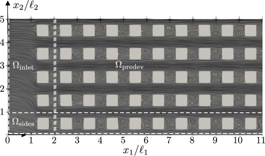
Figure 1: Flow velocity field in the mid plane $x_{3}=H/2$ of a channel containing an array of in-line square cylinders ($N_{1}=20,N_{2}=10$, $s_{0}/\ell_{1}=1,s_{N}/\ell_{1}=10$, $H/\ell_{1}=1$, $\ell_{1}/\ell_{2}=1$) for $\mbox{\it Re}=50$ and $\epsilon_{f}=0.75$. The flow patterns and wakes have been visualized using line integral convolution (LIC) vector field visualization.

Figure 1 illustrates the velocity field that is obtained for the previous boundary conditions, in the mid plane of a channel containing an array of $20\times 10$ in-line square cylinders, for a Reynolds number $\mbox{\it Re}\triangleq\rho_{f}u_{b}2H/\mu_{f}=50$ and a porosity $\epsilon_{f}=0.75$. Because the flow is symmetric with respect to the plane $x_{2}=W/2$, only a part of the mid plane is shown. It can be seen from the flow patterns and the wakes behind each cylinder, that at $x_{1}/\ell_{1}\simeq 11$, the flow has almost become periodically developed. In this case, the direct numerical simulation was performed on a regularly-sized mesh of about $98$ millon mesh cells, resulting in a computational time of about $6$ hours on $13$ nodes of each $36$ processors, for a total number of $2500$ discrete time steps until a steady state was observed at time $t=20\ell_{1}/u_{b}$. The flow simulation was started from a uniform zero velocity field as initial condition. A mesh-refinement study has been carried out, to ensure that the estimated discretisation error on the local velocity profiles was at least below $2.5\%$. For all other direct numerical simulations presented in this work, the discretisation error has been estimated to have the same relative magnitude.

For the direct numerical simulation of the flow equations and their boundary conditions, the software package FEniCSLab was developed within the finite-element framework FEniCS (Alnaes et al. (2015)). The package FEniCSLab contains an object-oriented re-implementation of the parallel fractional-step solver of Oasis developed by Mortensen & Valen-Sendstad (2015) for the unsteady incompressible Navier-Stokes equations, and has been modified to allow for variable time stepping and coupled mass and heat transfer between a fluid and a (moving) solid. The discretization of the Navier-Stokes equations in FEniCSLab relies on piecewise quadratic Lagrange elements for the velocity and piecewise linear Lagrange elements for the pressure, so that almost fourth-order accuracy in velocity and second-order in pressure accuracy is achieved (Mortensen & Valen-Sendstad (2015)) on the regularly-sized meshes used in this work.

3 Macro-Scale Flow Equations for Steady Channel Flow

The macro-scale velocity field $\langle\boldsymbol{u}\rangle_{m}$ and macro-scale pressure field $\langle p\rangle_{m}$ in the channel are obtained by applying a spatial averaging operator or filter $\langle\;\rangle_{m}$ to the velocity and pressure distributions $\boldsymbol{u}$ and $p$, which follow from a direct numerical simulation of the Navier-Stokes equations. As we consider steady channel flow, they satisfy the following macro-scale Navier-Stokes equations,

$$\rho_{f}\boldsymbol{\nabla}\boldsymbol{\cdot}\left(\epsilon_{fm}^{-1}\langle\boldsymbol{u}\rangle_{m}\langle\boldsymbol{u}\rangle_{m}\right) =-\boldsymbol{\nabla}\langle p\rangle_{m}+\mu_{f}\nabla^{2}\langle\boldsymbol{u}\rangle_{m}-\rho_{f}\boldsymbol{\nabla}\boldsymbol{\cdot}{\boldsymbol{M}}+\boldsymbol{b}\,,$$ (2)

$$\boldsymbol{\nabla}\boldsymbol{\cdot}\langle\boldsymbol{u}\rangle_{m} =0\,.$$ (3)

Here, $\epsilon_{fm}\triangleq\langle\gamma_{f}\rangle_{m}$ is the weighted porosity, and $\boldsymbol{M}\triangleq\langle\boldsymbol{u}\boldsymbol{u}\rangle_{m}-\epsilon_{fm}^{-1}\langle\boldsymbol{u}\rangle_{m}\langle\boldsymbol{u}\rangle_{m}$ the macro-scale momentum dispersion tensor. The closure force $\boldsymbol{b}$ results from the no-slip condition (1) at the channel walls and the fluid-solid interface:

$$\boldsymbol{b}\triangleq\langle\boldsymbol{n}_{0}\boldsymbol{\cdot}(-p_{f}\boldsymbol{I}+\boldsymbol{\tau}_{f})\delta_{0}\rangle_{m}\,.$$ (4)

We remark that $\boldsymbol{I}$ denotes the identity tensor and $\boldsymbol{n}_{0}$ denotes the normal at $\Gamma_{0}$ (pointing towards $\Omega_{s}$ at $\Gamma_{fs}$ and pointing outwards $\Omega$ at $\Gamma$), while $\delta_{0}$ is the Dirac surface indicator of the no-slip surface $\Gamma_{0}$. The filter operator itself is defined by the convolution product in $\mathbb{R}^{3}$ with a compact weighting function $m$: $\langle\boldsymbol{\phi}\rangle_{m}\triangleq m\ast\boldsymbol{\phi}$ (Quintard & Whitaker (1994b); Buckinx (2017)).

In order that $\langle\boldsymbol{u}\rangle_{m}$ and $\langle p\rangle_{m}$, as well as their governing equations (2) and (3), be defined on the entire domain $\Omega$, $\boldsymbol{u}$ and $p$ are defined here as extended distributions derived from the velocity $\boldsymbol{u}_{f}$ and pressure $p_{f}$ which appear in the original Navier-Stokes equations: $\boldsymbol{u}=\boldsymbol{u}_{f}\text{ in }\Omega_{f}$, $\boldsymbol{u}=0\text{ in }\Omega_{s}$, $\boldsymbol{u}=\boldsymbol{u}_{e}\text{ in }\mathbb{R}^{3}\setminus\Omega$ and $p=p_{f}\text{ in }\Omega_{f}$, $p=0\text{ in }\Omega_{s}$, $p=p_{e}\text{ in }\mathbb{R}^{3}\setminus\Omega$ (Schwartz (1978)). Therefore, also the viscous stress tensor $\boldsymbol{\tau}$ is a distribution given by $\boldsymbol{\tau}=\mu_{f}\left(\boldsymbol{\nabla}^{\nu}\boldsymbol{u}+\boldsymbol{\nabla}^{\nu}\boldsymbol{u}^{\intercal}\right)$, where $\boldsymbol{\nabla}^{\nu}$ denotes the gradient operator in the usual sense (Quintard & Whitaker (1994b); Gagnon (1970)). As shown in appendix A, a suitable choice of the extensions $\boldsymbol{u}_{e}$, $p_{e}$ and $\boldsymbol{\tau}_{e}$ has been made such that the form of the macro-scale flow equations (2) and (3) is valid.

In this work, the weighting function that is used to define the macro-scale flow, corresponds to a double volume average:

$$m(\boldsymbol{y})=\frac{1}{H}\operatorname{rect}\left(\frac{y_{3}}{H}\right)\displaystyle\prod_{j=1}^{2}\frac{l_{j}-2|y_{j}|}{l_{j}}\operatorname{rect}\left(\frac{y_{j}}{2\ell_{j}}\right)\qquad\mbox{with}~{}~{}y_{j}\triangleq\boldsymbol{y}\boldsymbol{\cdot}\boldsymbol{e}_{j}\,.$$ (5)

This weighting function has a compact support or filter window given by the local unit cell $\Omega_{\text{unit}}^{2\times 2}(\boldsymbol{x})$, which is defined by

$$\Omega_{\text{unit}}^{n_{1}\times n_{2}}(\boldsymbol{x})\triangleq\left\{\boldsymbol{r}=\boldsymbol{x}+\boldsymbol{y}\,|\,\exists\,c_{j}\in\left[-\frac{1}{2},\frac{1}{2}\right]\Leftrightarrow\boldsymbol{y}=\sum_{j=1}^{2}c_{j}n_{j}\boldsymbol{l}_{j}+c_{3}H\boldsymbol{e}_{3}\right\}\,.$$ (6)

Therefore, this weighting function enables an exact macro-scale description of periodically developed flow (Buckinx & Baelmans (2015b)), as long as the flow field is periodically similar within each unit cell $\Omega_{\text{unit}}^{n_{1}\times n_{2}}(\boldsymbol{x})$ with $n_{j}\leq 2$.

Because we only evaluate the filtered quantities at the mid plane $x_{3}=H/2$ of the channel, the centroid $\boldsymbol{x}$ of the filter window is chosen such that the window does not fall out the channel domain, i.e. $\forall\boldsymbol{r}\in\Omega_{\text{unit}}^{2\times 2}(\boldsymbol{x}):\boldsymbol{r}\in\Omega$. It must be remarked that we have chosen the height of the filter window equal to that of the channel, since the macro-scale flow then becomes two-dimensional, due to the no-slip condition at the bottom and top surface of the channel. Moreover, we remark that the filter based on the weighting function (5) is a separable filter whose action on the flow is equivalent to height-averaging followed by double volume averaging (Buckinx (2017)).

Further in this work, also the intrinsic averaging operator $\langle\;\rangle^{f}_{m}$ and deviation operator $(\,\widetilde{\;}\,)$ (Gray (1975))corresponding to the weighting function (5) are frequently used, whose definitions are given by $\langle\boldsymbol{\phi}\rangle^{f}_{m}\triangleq\epsilon_{fm}^{-1}\langle\boldsymbol{\phi}\rangle_{m}$ and $\widetilde{\boldsymbol{\phi}}\triangleq\boldsymbol{\phi}-\langle\boldsymbol{\phi}\rangle^{f}_{m}\gamma_{f}$. Each of the previous filter operators has been implemented in FEniCSLab as an explicit finite-element integral operator which can be applied to an arbitrary finite-element function. This discrete integral operator makes use of the automated quadrature degree estimation algorithms available in UFL (Alnaes et al. (2014)). For its parallel point-wise evaluation, a custom interpolation algorithm was written in DOLFIN (Logg & Wells (2010)) which is quite similar to the interpolation routines of the software package fenicstools by Mortensen (2017).

4 Macro-Scale Flow Regions in a Channel

From a macro-scale perspective, different flow regions can be identified in a channel containing an array of in-line equidistant square cylinders. These flow regions are illustrated in figure 2, which shows the macro-scale velocity field in a channel with an array of $20\times 10$ cylinders, for a Reynolds number $\mbox{\it Re}=50$. The macro-scale velocity components $\langle u_{j}\rangle^{f}_{m}\triangleq\langle\boldsymbol{u}\rangle^{f}_{m}\boldsymbol{\cdot}\boldsymbol{e}_{j}$ in figure 2 have been calculated via explicit filtering of the velocity field that was illustrated in figure 1. The explicit filtering operation for each velocity component took $12$ hours on $3$ nodes of $36$ processors.

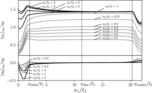
Figure 2: Macro-scale velocity components and flow regions in a channel array ($N_{1}=20,N_{2}=10$, $s_{0}/\ell_{1}=1,s_{N}/\ell_{1}=10$, $H/\ell_{1}=1$, $\ell_{1}/\ell_{2}=1$) for $\mbox{\it Re}=50$ and $\epsilon_{f}=0.75$. Grey and black lines correspond to locations inside and outside the side-wall region respectively.

The first flow region we identify in figure 2, is the inlet region, $\Omega_{\text{inlet}}\triangleq\{\boldsymbol{x}\in\Omega|x_{1}\in(0,x_{\text{inlet}}),x_{\text{inlet}}=s_{0}+\ell_{1}\}$, which extends from the channel inlet to the cross section after the first cylinder row where the weighted porosity $\epsilon_{fm}$ does no longer vary with the coordinate $x_{1}$ in the main flow direction.

Secondly, there is the outlet region, $\Omega_{\text{outlet}}\triangleq\{\boldsymbol{x}\in\Omega|x_{1}\in(x_{\text{outlet}},L),x_{\text{outlet}}=L-s_{N}-\ell_{1}\}$, which extends from the channel outlet to the cross section before the last cylinder row where a gradient of the weighted porosity starts to occur in the main flow direction $x_{1}$.

Between the inlet region and outlet region, we distinguish the channel’s core region, $\Omega_{\text{core}}\triangleq\{\boldsymbol{x}\in\Omega|x_{1}\in\left[x_{\text{inlet}},x_{\text{outlet}}\right]\}$. In this region, the weighted porosity $\epsilon_{fm}$ is constant everywhere, except in the region near the side walls, $\Omega_{\text{sides}}\triangleq\{\boldsymbol{x}\in\Omega|x_{2}\in((0,\ell_{2})\cup(W-\ell_{2},W))\}$, where $\epsilon_{fm}$ depends on the coordinate $x_{2}$ and decreases towards $\Gamma_{\text{sides}}$.

In the channel’s core region, typically a periodically developed flow region $\Omega_{\text{periodic}}\triangleq\{\boldsymbol{x}\in\Omega|x_{1}\in\left[x_{\text{periodic}},x_{\text{end}}\right]\}$ is established, provided that the number of solid cylinders $N_{1}$ along the main flow direction is sufficiently large with respect to the Reynolds number Re and no flow transition caused by vortex shedding occurs. In the periodically developed flow region, the velocity distribution can be treated as spatially periodic in the main flow direction, i.e.

$$\boldsymbol{u}(\boldsymbol{x}+n_{1}\boldsymbol{l}_{1})=\boldsymbol{u}(\boldsymbol{x})\qquad\mbox{for}~{}~{}\boldsymbol{x}\in\Omega_{\text{periodic}}\,,$$ (7)

with $n_{1}$ some integer. As a consequence, the macro-scale velocity has the same profile $U_{\text{dev}}(x_{2})$ over every cross section in $\Omega_{\text{periodic}}$ which is located at a distance larger than $n_{1}\ell_{1}$ from the onset point and end point of flow periodicity. Hence,

$$\langle\boldsymbol{u}\rangle_{m}(\boldsymbol{x})=\boldsymbol{U}_{\text{dev}}(\boldsymbol{x})\triangleq U_{\text{dev}}(x_{2})\boldsymbol{e}_{1}\qquad\mbox{for}~{}~{}\boldsymbol{x}\in\Omega_{\text{dev}}\,,$$ (8)

with $\Omega_{\text{dev}}\triangleq\{\boldsymbol{x}\in\Omega|x_{1}\in(x_{\text{dev}},x_{\text{end}}-n_{1}\ell_{1})\}$ and $x_{\text{dev}}\triangleq x_{\text{periodic}}+n_{1}\ell_{1}$. For that reason, the macro-scale velocity is called developed in $\Omega_{\text{dev}}$. We remark that the end point of flow development in good approximation satisfies $x_{\text{end}}\simeq x_{\text{outlet}}$ for the flow conditions and array geometries investigated in this work (Buckinx (2022)). It is well known (Patankar et al. (1977)) that because of (7), the pressure distribution in $\Omega_{\text{periodic}}$ has the form

$$p(\boldsymbol{x})=(\boldsymbol{\nabla}\mathrm{P}_{\text{dev}}\boldsymbol{\cdot}\boldsymbol{x})\gamma_{f}(\boldsymbol{x})+p^{\star}(\boldsymbol{x})\qquad\mbox{with}\qquad p^{\star}(\boldsymbol{x}+n_{1}\boldsymbol{l}_{1})=p^{\star}(\boldsymbol{x})\,.$$ (9)

Here, $\boldsymbol{\nabla}\mathrm{P}_{\text{dev}}$ denotes the constant pressure gradient which drives the periodically developed flow.

The velocity distribution in $\Omega_{\text{periodic}}$ also exhibits transversal periodicity at a distance larger than $\ell_{\text{sides}}$ from $\Gamma_{\text{sides}}$, if the number of solid cylinders $N_{2}$ in the transversal direction is sufficiently large. In that case, we thus have

$$\boldsymbol{u}(\boldsymbol{x}+n_{2}\boldsymbol{l}_{2})=\boldsymbol{u}(\boldsymbol{x})\qquad\mbox{and}\qquad p^{\star}(\boldsymbol{x}+n_{2}\boldsymbol{l}_{2})=p^{\star}(\boldsymbol{x})\,,$$ (10)

for all $\boldsymbol{x}\in\Omega_{\text{periodic}}$ with $x_{2}\in(\ell_{\text{sides}},W-\ell_{\text{sides}})$ and for some integer $n_{2}$. As a result, the developed macro-scale velocity field becomes uniform at a distance of $\ell_{\text{sides}}+n_{2}\ell_{2}$ from $\Gamma_{\text{sides}}$, so that

$$\boldsymbol{U}_{\text{dev}}(\boldsymbol{x})=\boldsymbol{U}\triangleq U\boldsymbol{e}_{1}\qquad\mbox{for}~{}~{}\boldsymbol{x}\in\Omega_{\text{uniform}}\,,$$ (11)

as $\Omega_{\text{uniform}}\triangleq\{\boldsymbol{x}\in\Omega|x_{1}\in(x_{\text{dev}},x_{\text{end}}-n_{1}\ell_{1}),x_{2}\in(\ell_{\text{sides}}+n_{2}\ell_{2},W-\ell_{\text{sides}}-n_{2}\ell_{2})\}$.

The last region we identify in $\Omega_{\text{core}}$, is the developing-flow region $\Omega_{\text{predev}}\triangleq\{\boldsymbol{x}\in\Omega|x_{1}\in\left[x_{\text{inlet}},x_{\text{dev}}\right]\}$, which precedes the periodically developed flow region. Now that the different macro-scale flow regions for the filter (5) have been defined, we will introduce the region of quasi-developed macro-scale flow.

5 Quasi-Developed Macro-Scale Flow

After a certain section in the developing-flow region $\Omega_{\text{predev}}$, the flow can be described as quasi-periodically developed (Buckinx (2022)). This means that the velocity distribution $\boldsymbol{u}$ converges asymptotically towards a truly periodic velocity distribution $\boldsymbol{u}^{\star}$ along the main flow direction via a single exponential mode:

$$\boldsymbol{u}=\boldsymbol{\mathsf{U}}\exp\left(-\boldsymbol{\lambda}\boldsymbol{\cdot}\boldsymbol{x}\right)+\boldsymbol{u}^{\star}\,,$$ (12)

where $\boldsymbol{u}^{\star}(\boldsymbol{x}+n_{1}\boldsymbol{l}_{1})=\boldsymbol{u}^{\star}(\boldsymbol{x})$ and

$$\boldsymbol{\mathsf{U}}(\boldsymbol{x}+n_{1}\boldsymbol{l}_{1})=\boldsymbol{\mathsf{U}}(\boldsymbol{x})\,.$$ (13)

The eigenvalue $\boldsymbol{\lambda}\triangleq\lambda\boldsymbol{e}_{1}$ and the mode amplitude $\boldsymbol{\mathsf{U}}$ are the solution of the eigenvalue problem given in (Buckinx (2022)). The region over which the flow is quasi-periodically developed, is denoted by $\Omega_{\text{quasi-periodic}}\triangleq\{\boldsymbol{x}\in\Omega|x_{1}\in\left[x_{\text{quasi-periodic}},x_{\text{periodic}}\right]\}$ and $x_{\text{quasi-periodic}}$ is called the onset point of quasi-periodically developed flow. In agreement with (9), the pressure field in $\Omega_{\text{quasi-periodic}}$ is given by

$$p_{f}(\boldsymbol{x})=\mathsf{P}_{f}(\boldsymbol{x})\exp\left(-\boldsymbol{\lambda}\boldsymbol{\cdot}\boldsymbol{x}\right)+\boldsymbol{\nabla}\mathrm{P}_{\text{dev}}\boldsymbol{\cdot}\boldsymbol{x}+p^{\star}_{f}(\boldsymbol{x})\,,$$ (14)

where

$$\mathsf{P}(\boldsymbol{x}+n_{1}\boldsymbol{l}_{1})=\mathsf{P}(\boldsymbol{x})\,.$$ (15)

The magnitude of the modes $\boldsymbol{\mathsf{U}}$ and $\mathsf{P}$ is characterized by a single constant $C_{\boldsymbol{\mathsf{U}}}\triangleq\langle{\mathsf{U}_{1}}\rangle_{\text{row}}$, which is the row-wise average of ${\mathsf{U}_{1}}$. This constant $C_{\boldsymbol{\mathsf{U}}}$ is called the perturbation size and depends on the specific inlet conditions (Buckinx (2022)).

It follows from (12) that the quasi-developed macro-scale flow field satisfies

$$\langle\boldsymbol{u}\rangle_{m}\simeq\boldsymbol{U}_{\text{dev}}+\langle\boldsymbol{\mathsf{U}}\rangle_{m}\exp\left(-\lambda x_{1}\right)\,,$$ (16)

since $\boldsymbol{U}_{\text{dev}}\triangleq\langle\boldsymbol{u}^{\star}\rangle_{m}$ in agreement with (7) and (8). Because of (13), it holds that

$$\frac{\partial}{\partial x_{1}}\langle\boldsymbol{\mathsf{U}}\rangle_{m}=0\,,$$ (17)

so the amplitude $\langle\boldsymbol{\mathsf{U}}\rangle_{m}$ of the macro-scale velocity mode depends only on the coordinate $x_{2}$. The quasi-developed macro-scale pressure field corresponding to (16) is given by

$$\langle p\rangle^{f}_{m}\simeq\boldsymbol{\nabla}\mathrm{P}_{\text{dev}}\boldsymbol{\cdot}\left(\boldsymbol{x}+\boldsymbol{m}\right)+\langle p^{\star}\rangle^{f}_{m}+\langle\mathsf{P}\rangle^{f}_{m}\exp\left(-\boldsymbol{\lambda}\boldsymbol{\cdot}\boldsymbol{x}\right)\,,$$ (18)

if $\boldsymbol{m}$ denotes the first intrinsic spatial moment over the fluid region (Quintard & Whitaker (1994a); Davit & Quintard (2017)). As a technical note, we remark that (16) and (18) are approximations instead of equalities, unless the filter’s weighting function is matched to the eigenvalue $\lambda$, as discussed in (Buckinx & Baelmans, 2015a). However, for the double volume-averaging operator (5), the latter approximations are sufficiently accurate as long as $\lambda\ell_{1}\ll 1$. Otherwise, the filter operator $\langle\;\rangle_{m}$ should be interpreted as a matched filter.

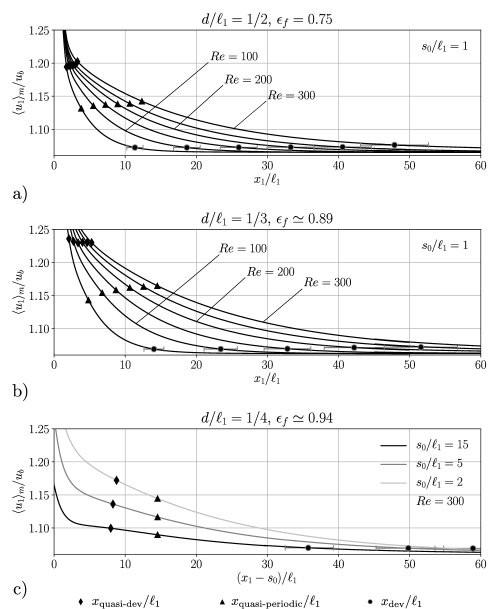
Figure 3: Macro-scale velocity profiles along the centreline ($x_{2}=W/2$) of a channel array ($N_{1}=80,N_{2}=10$, $H/\ell_{1}=1$, $\ell_{1}/\ell_{2}=1$, $s_{N}/\ell_{1}=10$) for different Reynolds numbers $\mbox{\it Re}\in\left\{50,100,150,200,250,300\right\}$ and porosities $\epsilon_{f}$, as well as different positions $s_{0}$ of the first cylinder row. The onset point of quasi-periodically developed flow, $x_{\text{quasi-periodic}}/\ell_{1}$, is shown together with the onset point of quasi-developed macro-scale flow, $x_{\text{quasi-dev}}/\ell_{1}$, as well as the point of developed flow, $x_{\text{dev}}/\ell_{1}$.

We may expect that the macro-scale velocity field can be treated as quasi-developed even before the local velocity field has become quasi-periodically developed in the strict sense of (12) and (13). This means that (16) and (17) are already an accurate approximation after a certain section $x_{1}=x_{\text{quasi-dev}}$ with $x_{\text{quasi-dev}}\leq x_{\text{quasi-periodic}}$. The reason is that an exponential mode $\boldsymbol{A}(\boldsymbol{x})\exp(-\lambda x_{1})$ with $\boldsymbol{A}(\boldsymbol{x})\simeq\boldsymbol{\mathsf{U}}(\boldsymbol{x})$ is already present within the velocity field $\boldsymbol{u}_{f}$ at the start of the flow development, near $x_{1}\simeq x_{\text{inlet}}$, so that after spatial averaging, it may pop up as a dominant mode in the macro-scale velocity field $\langle\boldsymbol{u}\rangle_{m}$, even before it has become the dominant mode for $\boldsymbol{u}_{f}$.

The latter expectation is also supported by the numerical evidence in figure 3, which shows an exponential evolution of the macro-scale velocity, $\langle u_{1}\rangle_{m}=\langle A_{1}\rangle_{m}\exp(-\lambda x_{1})+U_{\text{dev},1}$ with $\partial\langle A_{1}\rangle_{m}/\partial x_{1}\simeq 0$, from a section $x_{1}=x_{\text{quasi-dev}}$ relatively close to the inlet region, as indicated by the markers ($\mathrel{\scalebox{0.7}{$\blacklozenge$}}$). In a strict sense though, $\partial\langle A_{1}\rangle_{m}/\partial x_{1}=0$ is only valid when $\langle A_{1}\rangle_{m}=\langle{\mathsf{U}_{1}}\rangle_{m}$, which is the case for $x_{1}>x_{\text{quasi-periodic}}$, hence after the sections indicated by the markers ($\mathrel{\scalebox{0.9}{$\blacktriangle$}}$). We clarify that the macro-scale velocity profiles in figure 3 have been obtained by explicit filtering of the velocity fields from our preceding work (Buckinx (2022)). The explicit filtering operation took $24$ hours on $3\times 36$ processors for just a single velocity component on each mesh of about $140$ million mesh cells.

In figure 3 (a,b), one can see that the onset point of quasi-developed macro-scale flow, $x_{\text{quasi-dev}}$, scales in good approximation linearly with the Reynolds number Re, just like the onset point of quasi-periodically developed flow, $x_{\text{quasi-periodic}}$ (Buckinx (2022)). For the channel geometries selected for this figure, i.e. for $H=\ell_{1}=\ell_{2}=s_{0}$ and $W/H=N_{2}=10$, it was found that $x_{\text{quasi-dev}}/\ell_{1}\simeq 0.006\mbox{\it Re}+1.5$ for $d/\ell_{1}=1/2$, while $x_{\text{quasi-dev}}/\ell_{1}\simeq 0.013\mbox{\it Re}+1.5$ for $d/\ell_{1}=1/3$, when $\mbox{\it Re}\in\left\{50,100,150,200,250,300\right\}$. These linear correlations for $x_{\text{quasi-dev}}/\ell_{1}$ have been determined numerically by defining $x_{\text{quasi-dev}}$ as the $x_{1}$-section for which $\langle u_{1}\rangle_{m}-U_{\text{dev},1}$ at $x_{2}=W/2$ deviates less than $99.9\%$ from the exponential relationship $\langle{\mathsf{U}_{1}}\rangle_{m}\exp(-\lambda x_{1})$. The relative uncertainty on these correlations is about $10\%$, as the uncertainty on the numerical values for $x_{\text{quasi-dev}}/\ell_{1}$ in figure 3, is within $10\%$ too.

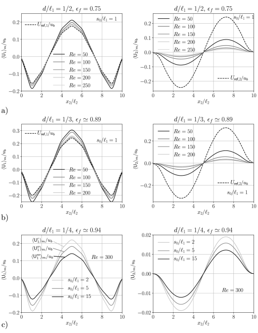
Figure 4: Macro-scale velocity modes for quasi-developed flow in a channel array ($N_{1}=80,N_{2}=10$, $H/\ell_{1}=1$, $\ell_{1}/\ell_{2}=1$, $s_{N}/\ell_{1}=10$) for different Reynolds numbers $\mbox{\it Re}\in\left\{50,100,150,200,250,300\right\}$ and porosities $\epsilon_{f}$, as well as different positions $s_{0}$ of the first cylinder row.

The dimensionless velocity modes $\langle\boldsymbol{\mathsf{U}}\rangle_{m}/u_{b}$ in the quasi-developed flow region for each of the channel flows depicted in figure 3 are shown in figure 4. Figure 4 (a,b) demonstrates that the shapes of the dimensionless macro-scale velocity modes at different Reynolds numbers are very similar when the inlet velocity profile and geometry of the channel and array remain unaltered. Therefore, their shapes can be represented by a Reynolds-number-independent reference profile $\boldsymbol{U}_{\text{ref}}(x_{2})/u_{b}$ such that

$$\frac{\langle\boldsymbol{\mathsf{U}}\rangle_{m}}{u_{b}}=\frac{\boldsymbol{U}_{\text{ref}}}{u_{b}}\left(1+\frac{c_{2}}{\mbox{\it Re}}\right)\boldsymbol{\cdot}\left(\boldsymbol{e}_{1}\boldsymbol{e}_{1}+\lambda\ell_{2}\boldsymbol{e}_{2}\boldsymbol{e}_{2}\right)\,.$$ (19)

This correlation form is based on the observation that the mode amplitude scales inversely linear with the Reynolds number: $\langle{\mathsf{U}_{1}}\rangle_{m}/u_{b}\sim(1+c_{2}/\mbox{\it Re})$. We have for instance $c_{2}\simeq 9.6$ for $d/\ell_{1}=1/2$, and $c_{2}\simeq 13$ for $d/\ell_{1}=1/3$, if $\ell_{1}/\ell_{2}=H/\ell_{1}=1$, $N_{2}=10$ and $s_{0}/\ell_{1}=1$. Furthermore, the form of this correlation takes into account that

$$\langle{\mathsf{U}_{2}}\rangle_{m}(x_{2})=\lambda\ell_{2}\displaystyle\int_{0}^{x_{2}/\ell_{2}}\langle{\mathsf{U}_{1}}\rangle_{m}(r_{2})dr_{2}\qquad\mbox{with}\qquad r_{2}\triangleq\frac{x_{2}}{\ell_{2}}\,,$$ (20)

due to the fact that $\boldsymbol{\nabla}\boldsymbol{\cdot}\boldsymbol{\mathsf{U}}=\boldsymbol{\lambda}\boldsymbol{\cdot}\boldsymbol{\mathsf{U}}$, by virtue of (3) and (16). We remark that (20) implies that only the component $U_{\text{ref,0}}$ and eigenvalue $\lambda$ are essential to reconstruct $\boldsymbol{U}_{\text{ref}}$.

Figure 4 (c) illustrates that the dimensionless macro-scale velocity modes for the same Reynolds number Re and same inlet velocity profile are all self-similar, apart from the scaling factor $C_{\boldsymbol{\mathsf{U}}}/u_{b}$. This scaling factor $C_{\boldsymbol{\mathsf{U}}}/u_{b}$, which determines the absolute value of the macro-scale velocity at the onset point $x_{\text{quasi-periodic}}/\ell_{1}$, clearly depends on the distance over which the flow is developing and thus the distance $s_{0}/\ell_{1}$ between the channel inlet and the first cylinder row, as one can observe in figure 3 (c). The perturbation size $C_{\boldsymbol{\mathsf{U}}}/u_{b}$ obviously increases when the flow has less distance to adapt itself to the array geometry, as the inlet profile has been fixed here.

The macro-scale velocity modes from figure 4 have some features in common with the two-dimensional velocity modes that occur in quasi-developed Poiseuille flow (Sadri & Floryan (2002); Asai & Floryan (2004)). The profile of $\langle{\mathsf{U}_{1}}\rangle_{m}/u_{b}$ has a similar W-shape over the width of the channel, while the profile of $\langle{\mathsf{U}_{2}}\rangle_{m}/u_{b}$ has a similar sinusoidal shape. In addition, the inversely linear relationship between the mode amplitude and the Reynolds number has also been discovered for quasi-developed Poiseuille flow at Reynolds numbers below 500 (Sadri (1997)). A difference, however, is that the modes of the macro-scale velocity do not satisfy a no-slip condition at the side walls of the channel. Besides, the modes from figure 4 differ in sign with respect to the modes observed in quasi-developed Poiseuille flow. The sign of the macro-scale velocity modes implies that the macro-scale velocity decreases along the center of the channel when the flow develops, whereas for quasi-developed Poiseuille flow, the velocity at the center of the channel tends to increase when the flow develops. The different sign of the perturbation size is an outcome of the specific inlet velocity profile and $s_{0}/\ell_{1}$-ratio chosen for the direct numerical simulation of the channel flow here. In figure 4 (a,b), the ratio $s_{0}/\ell_{1}$ is small, so that there occurs a velocity peak and overshoot of the macro-sale velocity in the center of the channel shortly after the flow enters the array. As figures 3 and 4 (c) show, this velocity peak decreases when $s_{0}/\ell_{1}$ increases. Eventually, when the distance between the channel inlet and first cylinder row becomes very large, a negative perturbation size, thus an undershoot of the macro-scale velocity at the center of the channel can be expected, in agreement with the experiments for quasi-developed Poiseuille flow (Asai & Floryan, 2004)).

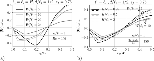
Figure 5: Macro-scale velocity modes for quasi-developed flow in a channel array ($N_{1}=60$, $\ell_{1}/\ell_{2}=1$, $s_{0}/\ell_{1}=1$, $s_{N}/\ell_{1}=10$) for different aspect ratios $W/\ell_{2}\in\left\{5,10,20,25\right\}$ (a) and height ratios $H/\ell_{1}\in\left\{0.25,0.5,0.25\right\}$ (b) of the channel. The porosity $\epsilon_{f}$ and the Reynolds number based on the cylinder spacing $2\rho_{f}u_{b}\ell_{1}/\mu_{f}$ have been kept fixed.

The influence of the geometry on the shape of the mode and the perturbation size is demonstrated in figure 5 for a single porosity and a single Reynolds number based on the cylinder spacing. Only half of the channel is shown, because the mode is symmetric with respect to the center plane $x_{1}=W/2$. In figure 5 (a), we can see that a larger aspect ratio $W/H=W/\ell_{2}$ comes along with a smaller perturbation size for the chosen inlet conditions. In addition, the location of the minimum of the mode $\langle{\mathsf{U}_{1}}\rangle_{m}$ moves closer to the side walls of the channel, when the aspect ratio increases. In figure 5 (b), we can see that a larger channel height comes along with a smaller perturbation size until $H/\ell_{1}>1$, after which the mode shape and perturbation remain constant. The influence of the channel height and the aspect ratio at the macro-scale is of course in line with the scaling laws for the velocity mode $\boldsymbol{\mathsf{U}}$, which are discussed in (Buckinx (2022)), so they are not treated here again.

In order to obtain an exact local closure problem for quasi-developed macro-scale flow, exact closure solutions for developed flow macro-scale flow need to be achieved first. Such closure solutions are presented in the next section, for the region of uniform macro-scale flow. Afterwards, they are extended to include the side-wall region.

6 Local Closure for Developed Macro-Scale Flow

6.1 Exact Local Closure in the Region of Uniform Macro-Scale Flow

In the region $\Omega_{\text{uniform}}$, where the macro-scale velocity $\boldsymbol{U}$ is uniform, also the closure force $\boldsymbol{b}$ adopts a uniform value, which is given by

$$\boldsymbol{b}^{\star}\triangleq\langle\boldsymbol{n}_{0}\boldsymbol{\cdot}(-p^{\star}_{f}\boldsymbol{I}+\mu_{f}\boldsymbol{\nabla}\boldsymbol{u}^{\star}_{f})\delta_{0}\rangle_{m}\,.$$ (21)

Following the derivations from Buckinx & Baelmans (2015b), it can be proved that the uniform closure force (21) is exactly represented by a spatially independent apparent permeability tensor $\boldsymbol{K}_{\text{uniform}}\left(\boldsymbol{U}\right)$, which depends on $\boldsymbol{U}$:

$$\boldsymbol{b}^{\star}=-\mu_{f}\boldsymbol{K}^{-1}_{\text{uniform}}\boldsymbol{\cdot}\boldsymbol{U}\,.$$ (22)

The latter apparent permeability tensor is determined by the closure variables ${\boldsymbol{\Phi}^{\star}}$ and ${\boldsymbol{\varphi}^{\star}}$, which define the mappings $\boldsymbol{u}^{\star}(\boldsymbol{r})={\boldsymbol{\Phi}^{\star}}(\boldsymbol{r})\boldsymbol{\cdot}\boldsymbol{U}^{\prime}$ and $p^{\star}(\boldsymbol{r})=\mu_{f}{\boldsymbol{\varphi}^{\star}}(\boldsymbol{r})\boldsymbol{\cdot}\boldsymbol{U}^{\prime}$:

$$\boldsymbol{K}^{-1}_{\text{uniform}}\triangleq\epsilon_{fm}^{-1}\langle\boldsymbol{n}_{0}\boldsymbol{\cdot}(\boldsymbol{I}{\boldsymbol{\varphi}_{f}^{\star}}-\boldsymbol{\nabla}{\boldsymbol{\Phi}_{f}^{\star}})\delta_{0}\rangle_{m}\,.$$ (23)

We note that, apart from the macro-scale velocity $\boldsymbol{U}\triangleq\epsilon_{f}\boldsymbol{U}^{\prime}$, $\boldsymbol{K}^{-1}_{\text{uniform}}$ thus also depends on the fluid properties $\mu_{f}$ and $\rho_{f}$, as well as the geometrical parametrization of $\Gamma_{0}$. Furthermore, since $\langle{\boldsymbol{\Phi}^{\star}}\rangle^{f}_{m}$ and $\langle{\boldsymbol{\varphi}^{\star}}\rangle^{f}_{m}$ are constant in $\Omega_{\text{uniform}}$, this apparent permeability tensor is equivalent to the one defined by the classical closure problem of Whitaker (1996):

$$\boldsymbol{K}^{-1}_{\text{uniform}}=\epsilon_{fm}^{-1}\langle\boldsymbol{n}_{0}\boldsymbol{\cdot}(\boldsymbol{I}{\widetilde{\boldsymbol{\varphi}}_{f}^{\star}}-\boldsymbol{\nabla}{\widetilde{\boldsymbol{\Phi}}_{f}^{\star}})\delta_{0}\rangle_{m}\,.$$ (24)

Because the uniform closure force equals the constant macro-scale pressure gradient in $\Omega_{\text{uniform}}$,

$$\boldsymbol{b}^{\star}=\boldsymbol{\nabla}\langle p\rangle_{m}=\boldsymbol{\nabla}\mathrm{P}_{\text{dev}}\epsilon_{f}\,,$$ (25)

as shown in (Buckinx & Baelmans (2015b)), both $\boldsymbol{b}^{\star}$ and $\boldsymbol{K}_{\text{uniform}}$ can be governed as a function of $\boldsymbol{U}$ by solving the periodically developed flow equations given in (Buckinx & Baelmans (2015b); Buckinx (2022)). Due to the periodicity conditions (7) and (10) in $\Omega_{\text{uniform}}$, the periodically developed flow equations need to be solved on just a single unit cell $\Omega_{\text{unit}}^{n_{1}\times n_{2}}(\boldsymbol{x})$ with $\boldsymbol{x}\in\Omega_{\text{uniform}}$. The result of this classical closure procedure, which has been adopted in many studies (see e.g. Refs), is illustrated in figure 6, for a channel with an array of equidistant in-line square cylinders.

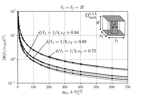
Figure 6: Magnitude of the closure force $\boldsymbol{b}=\boldsymbol{b}^{\star}$, as a function of the macro-scale velocity $U$ and porosity $\epsilon_{f}$ for a channel with an array of equidistant square in-line cylinders, in the region of uniform macro-scale flow. The solid lines correspond to the Darcy-Forchheimer relationship $(\ell_{1}^{2}/\kappa_{D})\mbox{\it Re}_{U}+\ell_{1}/\kappa_{F}$, while the dotted lines correspond to the Darcy relationship $(\ell_{1}^{2}/\kappa_{D})\mbox{\it Re}_{U}$.

Figure 6 shows the magnitude $\|\boldsymbol{b}^{\star}\|$ of the closure force in the region of uniform macro-scale flow, as a function of the macro-scale velocity $U$ and the porosity $\epsilon_{f}$ of the array. As mentioned earlier, a single height-to-spacing ratio $H/\ell_{1}=1$ has been chosen. The depicted data points, whose estimated accuracy is $1.5\%$ according to our mesh-refinement study, were obtained by numerically solving the periodically developed flow equations on a unit cell $\Omega_{\text{unit}}^{1\times 1}$, as the actual flow field in the channel is known to become periodic for $n_{1}=n_{2}=1$. Each unit-cell simulation was performed on a mesh of about $1.5$ million cells. Because we found numerically the same velocity field on $\Omega_{\text{unit}}^{1\times 1}$ whether $\boldsymbol{\nabla}\mathrm{P}_{\text{dev}}$ or $\boldsymbol{U}$ was imposed, so no flow bifurcations appeared, we argue that the relation between $\boldsymbol{b}$ and $\boldsymbol{U}$ is a one-to-one relationship over the range of Reynolds numbers $\mbox{\it Re}_{U}\triangleq 2\rho_{f}UH/\mu_{f}$ shown in figure 6. In agreement with the literature (e.g. Koch & Ladd (1997); Lasseux et al. (2011)), this one-to-one relationship satisfies in good approximation the Darcy-Forchheimer relationship,

$$\boldsymbol{b}^{\star}\simeq-\frac{\mu_{f}}{\kappa_{D}}\boldsymbol{U}-\frac{\rho_{f}}{\kappa_{F}}U\boldsymbol{U}\,,$$ (26)

so that $\|\boldsymbol{b}^{\star}\|\ell_{1}/(\rho_{f}U^{2})\simeq(\ell_{1}^{2}/\kappa_{D})/\mbox{\it Re}_{U}+\ell_{1}/\kappa_{F}$ and $\boldsymbol{K}^{-1}_{\text{uniform}}\simeq\left(\kappa_{D}^{-1}+\rho_{f}U/(\mu_{f}\kappa_{F})\right)\boldsymbol{I}$. By means of a least-square fitting procedure, the Darcy coefficient $\ell_{1}^{2}/\kappa_{D}$ was found to equal $233$ when $d/\ell_{1}=1/2$, $108$ when $d/\ell_{1}=1/3$, and $80$ when $d/\ell_{1}=1/4$ for the geometries and Reynolds numbers in figure 6. On the other hand, the corresponding Forchheimer coefficients were found to be much smaller: $\ell_{1}/\kappa_{F}=0.05$ for $d/\ell_{1}=1/2$, $\ell_{1}/\kappa_{F}=0.035$ for $d/\ell_{1}=1/3$, and $\ell_{1}/\kappa_{F}=0.03$ for $d/\ell_{1}=1/2$. With these values for the Darcy and Forchheimer coefficients, the relationship (26) deviates no more than $3$ to $5\%$ with respect to the data points depicted in figure 6, while its mean relative deviation is below $2\%$. Nevertheless, this relationship actually ignores the occurrence of a weak-inertia regime as discussed in (Lasseux et al. (2011)).

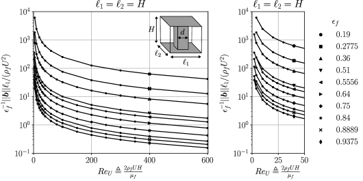
Figure 7: Magnitude of the closure force = as a function of the macro-scale velocity $U$ and porosity $\epsilon_{f}$, for a channel with an array of equidistant square in-line cylinders, in the region of uniform macro-scale flow.

The Darcy and Forchheimer coefficients can be correlated to the porosity of the array via the empirical formulas

$$\ell_{1}^{2}/\kappa_{D}=44.8\biggl{(}1-(1-\epsilon_{f})^{0.63}\biggr{)}^{-3}\qquad\mbox{and}\qquad\ell_{1}/\kappa_{F}=0.13\left(\frac{1-\epsilon_{f}}{\epsilon_{f}^{2}}\right)\,,$$ (27)

when the cylinder spacing is equal to the channel height: $H=\ell_{1}=\ell_{2}$. These formulas predict the 200 data points for the closure force in figure (7) with a mean relative error of $2\%$ and a maximum relative error below $9\%$. The estimated discretization error on the data points is below $1.5$ to 2$\%$. The correlations (27) show that if inertia effects at the macro-scale are neglected by setting the Forchheimer coefficient to $\ell_{1}/\kappa_{F}=0$, the closure force is underestimated by almost $8\%$ at the highest Reynolds number $\mbox{\it Re}=300$. Inertia effects at the macro-scale will thus remain rather small for $H/\ell_{1}<1$, since $\ell_{1}/\kappa_{F}$ tends to decrease when the channel height decreases. Furthermore, for $H/\ell_{1}>1$, both the Darcy and Forchheimer coefficients are expected to become constant and independent of $H/\ell_{1}$ (Vangeffelen et al. (2021)).

6.2 Exact Local Closure in the Region of Developed Macro-Scale Flow

In order to extend the former closure solutions towards the entire region of developed macro-scale flow $\Omega_{\text{dev}}$, we can express the closure force $\boldsymbol{b}$ explicitly in terms of the periodically developed velocity and pressure fields via (9):

$$\boldsymbol{b}_{\text{dev}}=\boldsymbol{b}^{\star}+\langle p\rangle^{f}_{m}\boldsymbol{\nabla}\epsilon_{fm}-\langle p^{\star}\rangle^{f}_{m}\boldsymbol{\nabla}\epsilon_{fm}-\epsilon_{fm}\boldsymbol{G}_{m}\boldsymbol{\cdot}\boldsymbol{\nabla}\mathrm{P}_{\text{dev}}\,.$$ (28)

Here, the developed macro-scale pressure field is given by

$$\langle p\rangle^{f}_{m}=\boldsymbol{\nabla}\mathrm{P}_{\text{dev}}\boldsymbol{\cdot}(\boldsymbol{x}+\boldsymbol{m})+\langle p^{\star}\rangle^{f}_{m}\,,$$ (29)

and $\boldsymbol{G}_{m}\triangleq-\nabla\boldsymbol{m}$ denotes the gradient of the first intrinsic spatial moment over the fluid region $\boldsymbol{m}$ (Buckinx & Baelmans (2015b); Quintard & Whitaker (1994a)). Additionally, we remark that although $\boldsymbol{b}^{\star}$ in (28) is still defined by (21), its value is no longer spatially uniform in $\Omega_{\text{dev}}$, so that (22) does not hold here.

We will now show that the closure force in the developed flow region (28) can be represented by an exact, yet spatially dependent, apparent permeability tensor $\boldsymbol{K}_{\text{dev}}\left(\boldsymbol{U}_{\text{dev}},x_{2}\right)$, such that

$$\boldsymbol{b}_{\text{dev}}=\langle p\rangle^{f}_{m}\boldsymbol{\nabla}\epsilon_{fm}-\mu_{f}\boldsymbol{K}_{\text{dev}}^{-1}\boldsymbol{\cdot}\boldsymbol{U}_{\text{dev}}\,.$$ (30)

To this end, we introduce the closure variable $\boldsymbol{\xi}$, which maps at each position in $\Omega_{\text{dev}}$, the uniform macro-scale velocity $\boldsymbol{U}^{\prime}$ to the actual macro-scale velocity $\boldsymbol{U}^{\prime}_{\text{dev}}\triangleq\epsilon_{fm}^{-1}\boldsymbol{U}_{\text{dev}}$:

$$\boldsymbol{U}_{\text{dev}}^{\prime}(x_{2})\triangleq\boldsymbol{\xi}\left(\boldsymbol{U},x_{2}\right)\boldsymbol{\cdot}\boldsymbol{U}^{\prime}\qquad\mbox{and}\qquad\xi\left(x_{2}\right)\triangleq\frac{U_{\text{dev}}^{\prime}(x_{2})}{U^{\prime}}\,.$$ (31)

The closure variable $\boldsymbol{\xi}=\xi\boldsymbol{I}$ thus determines the shape $\xi$ of the macro-scale velocity profile in $\Omega_{\text{dev}}$. We remark that $\boldsymbol{\xi}$ is solely a function of $\boldsymbol{U}$, if the fluid properties and geometry of $\Gamma_{0}$ are fixed. After all, $\boldsymbol{u}_{f}^{\star}$, $p_{f}^{\star}$ and hence $\boldsymbol{U}_{\text{dev}}$ in $\Omega_{\text{dev}}$ can be obtained, at least in principle, by solving the periodically developed flow equations on one or two rows of the array, for a fixed value of $\boldsymbol{U}$ (Buckinx (2022)).

With the aid of $\boldsymbol{\xi}$, we can define $\boldsymbol{K}_{\text{dev}}$ in $\Omega_{\text{dev}}$ in terms of the same closure mapping as the one that was introduced to define $\boldsymbol{K}_{\text{uniform}}$ in $\Omega_{\text{uniform}}$ (23):

$$\boldsymbol{u}(\boldsymbol{r}) ={\boldsymbol{\Phi}^{\star}}(\boldsymbol{r})\boldsymbol{\cdot}\boldsymbol{U}^{\prime}={\boldsymbol{\Phi}^{\star}}(\boldsymbol{r})\boldsymbol{\cdot}\boldsymbol{\xi}^{-1}\left(\boldsymbol{U},x_{2}\right)\boldsymbol{\cdot}\boldsymbol{U}_{\text{dev}}^{\prime}(x_{2})\,,$$ (32)

$$p^{\star}(\boldsymbol{r}) =\mu_{f}{\boldsymbol{\varphi}^{\star}}(\boldsymbol{r})\boldsymbol{\cdot}\boldsymbol{U}^{\prime}=\mu_{f}{\boldsymbol{\varphi}^{\star}}(\boldsymbol{r})\boldsymbol{\cdot}\boldsymbol{\xi}^{-1}\left(\boldsymbol{U},x_{2}\right)\boldsymbol{\cdot}\boldsymbol{U}_{\text{dev}}^{\prime}(x_{2})\,.$$

Substitution of the closure mapping (32) in the expression for the closure force yields for the first term on the right-hand side of (28):

$$\boldsymbol{b}^{\star}=-\mu_{f}\epsilon_{fm}^{-1}\langle\boldsymbol{n}_{0}\boldsymbol{\cdot}\left(\boldsymbol{I}{\boldsymbol{\varphi}_{f}^{\star}}-\boldsymbol{\nabla}{\boldsymbol{\Phi}_{f}^{\star}}\right)\delta_{0}\rangle_{m}\boldsymbol{\cdot}\boldsymbol{\xi}^{-1}\boldsymbol{\cdot}\boldsymbol{U}_{\text{dev}}\,.$$ (33)

For the third term on the right-hand side of (28), we obtain

$$\langle p^{\star}\rangle^{f}_{m}\boldsymbol{\nabla}\epsilon_{fm}=\mu_{f}\epsilon_{fm}^{-1}\boldsymbol{\nabla}\epsilon_{fm}\langle{\boldsymbol{\varphi}^{\star}}\rangle^{f}_{m}\boldsymbol{\cdot}\boldsymbol{\xi}^{-1}\boldsymbol{\cdot}\boldsymbol{U}_{\text{dev}}\,.$$ (34)

Furthermore, substitution of (32) in the last term of (28) results in

$$\epsilon_{fm}\boldsymbol{G}_{m}\boldsymbol{\cdot}\boldsymbol{\nabla}\mathrm{P}_{\text{dev}}=\mu_{f}\boldsymbol{G}_{m}\boldsymbol{\cdot}\boldsymbol{K}^{-1}_{\text{uniform}}\boldsymbol{\cdot}\boldsymbol{\xi}^{-1}\boldsymbol{\cdot}\boldsymbol{U}_{\text{dev}}\,,$$ (35)

by virtue of (22) and (23). Finally, we retrieve from (33) - (35) that the apparent permeability tensor in the developed flow region (30) is given by

$$\boldsymbol{K}_{\text{dev}}^{-1}=\left(\boldsymbol{K}^{-1}_{\text{dev,main}}+\boldsymbol{G}_{m}\boldsymbol{\cdot}\boldsymbol{K}^{-1}_{\text{uniform}}\right)\boldsymbol{\cdot}\boldsymbol{\xi}^{-1}\,,$$ (36)

where $\boldsymbol{\xi}=\langle{\boldsymbol{\Phi}^{\star}}\rangle^{f}_{m}$ and

$$\boldsymbol{K}^{-1}_{\text{dev,main}}\triangleq\epsilon_{fm}^{-1}\langle\boldsymbol{n}_{0}\boldsymbol{\cdot}\left(\boldsymbol{I}{\boldsymbol{\varphi}_{f}^{\star}}-\boldsymbol{\nabla}{\boldsymbol{\Phi}_{f}^{\star}}\right)\delta_{0}\rangle_{m}+\epsilon_{fm}^{-1}\boldsymbol{\nabla}\epsilon_{fm}\langle{\boldsymbol{\varphi}^{\star}}\rangle^{f}_{m}\,.$$ (37)

In order to determine $\boldsymbol{K}_{\text{dev,main}}$ and $\boldsymbol{\xi}$, the closure problem (82) from appendix B must be solved on (a part of) the side-wall region in $\Omega_{\text{dev}}$.

We note that the functional dependence of $\boldsymbol{K}_{\text{dev}}$ on $\boldsymbol{U}=\epsilon_{f}\boldsymbol{U}^{\prime}$ is easily transformed into a functional dependence on $\boldsymbol{U}_{\text{dev}}$ via (31), so the notations $\boldsymbol{K}_{\text{dev}}\left(\boldsymbol{U},x_{2}\right)$, $\boldsymbol{K}_{\text{dev}}\left(\boldsymbol{U}^{\prime},x_{2}\right)$ and $\boldsymbol{K}_{\text{dev}}\left(\boldsymbol{U}_{\text{dev}},x_{2}\right)$ are all equivalent. Evidently, if $\boldsymbol{x}\in\Omega_{\text{uniform}}$, it holds that $\xi\left(\boldsymbol{U},x_{2}\right)=1$ and $\boldsymbol{G}_{m}=0$ (Buckinx & Baelmans (2015b)), so that in $\Omega_{\text{uniform}}$ we recover again $\boldsymbol{K}_{\text{dev}}\left(\boldsymbol{U},x_{2}\right)=\boldsymbol{K}_{\text{dev,main}}\left(\boldsymbol{U},x_{2}\right)=\boldsymbol{K}_{\text{uniform}}\left(\boldsymbol{U}\right)$, in agreement with (23).

6.3 Approximative Local Closure in the Region of Developed Macro-Scale Flow

Although the exact definition (36) may be interesting in itself for theoretical reasons, it has limited practical value due to the complexity of the closure problem (82). Nevertheless, it can be used as a starting point for accomplishing approximative closure. Hereto, we first assume that $\boldsymbol{G}_{m}\simeq 0$, or

$$\boldsymbol{K}_{\text{dev}}\simeq\boldsymbol{\xi}\boldsymbol{\cdot}\boldsymbol{K}_{\text{dev,main}}\,,$$ (38)

since the spatial moment $\boldsymbol{m}$ of the cylinder array in $\Omega_{\text{sides}}$ can be neglected for the double volume-averaging filter of (5). Secondly, we assume that the variation of $\langle{\boldsymbol{\varphi}^{\star}}\rangle^{f}_{m}$ with $x_{2}$ in the region $\Omega_{\text{dev}}\setminus\Omega_{\text{uniform}}$ is small, so that $\langle{\boldsymbol{\varphi}^{\star}}\rangle^{f}_{m}$ can be treated as a constant and be moved within the averaging operator $\langle\;\rangle_{m}$:

$$\boldsymbol{K}^{-1}_{\text{dev,main}}\simeq\epsilon_{fm}^{-1}\langle\boldsymbol{n}_{0}\boldsymbol{\cdot}(\boldsymbol{I}{\widetilde{\boldsymbol{\varphi}}_{f}^{\star}}-\boldsymbol{\nabla}{\boldsymbol{\Phi}_{f}^{\star}})\delta_{0}\rangle_{m}\,.$$ (39)

Also the assumption that $\langle{\boldsymbol{\varphi}^{\star}}\rangle^{f}_{m}(x_{2})$ is virtually constant, is not so restrictive, as it implies that the constant macro-scale pressure gradient outside the side-wall region is maintained within the side-wall region: $\boldsymbol{\nabla}\langle p\rangle^{f}_{m}\simeq\boldsymbol{\nabla}\mathrm{P}_{\text{dev}}$ because of $\boldsymbol{\nabla}\langle p^{\star}\rangle^{f}_{m}\simeq 0$ in $\Omega_{\text{dev}}$. If we compare (39) with (23) and (24), we see that we thus may use the approximation

$$\boldsymbol{K}_{\text{dev,main}}\simeq\boldsymbol{K}_{\text{uniform}}\qquad\mbox{or}\qquad\boldsymbol{K}_{\text{dev}}\simeq\boldsymbol{\xi}\boldsymbol{\cdot}\boldsymbol{K}_{\text{uniform}}\,,$$ (40)

provided that the variation of $\boldsymbol{K}_{\text{dev,main}}$ with $x_{2}$ is much smaller than the variation of $\xi$ with $x_{2}$ in the side-wall region $\Omega_{\text{sides}}$, or more precisely the region $\Omega_{\text{dev}}\setminus\Omega_{\text{uniform}}$. This last condition is true as long as $\boldsymbol{b}\simeq\boldsymbol{\nabla}\mathrm{P}_{\text{dev}}$ in $\Omega_{\text{dev}}$, and holds for all the flow conditions and array geometries investigated in this work.

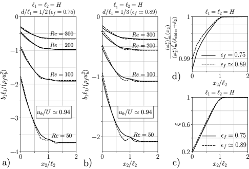
Figure 8: (a,b) Closure force for developed macro-scale flow in the side-wall region of a channel with an array of equidistant in-line cylinders, for different Reynolds numbers Re and different porosities $\epsilon_{f}$. The solid lines ($-$) represent the component $b_{1}$ of the actual closure force along the main flow direction. The dashed lines (- -) represent the approximation for $b_{1}$ given by (40). (c,d) Also the two closure variables $\xi$ and $\langle{\boldsymbol{\varphi}^{\star}}\rangle^{f}_{m}$ which determine the permeability tensor in the side-wall region are shown.

In practise, the approximation (40) is only useful if one knows or can estimate the shape of the developed macro-scale velocity profile $\xi$ a priori. Our numerical results indicate that in a channel array of square in-line cylinders, $\xi$ varies in a first approximation linearly with the coordinate $x_{2}$ perpendicular to the the side walls, so that

$$\xi\left(\boldsymbol{U},x_{2}\right)\simeq\left\{\begin{aligned} &\frac{x_{2}+\ell_{\text{slip}}}{\ell_{2}+\ell_{\text{slip}}}&&\qquad\mbox{for}~{}~{}x_{2}\in(0,\ell_{2})\,,\\ &~{}~{}~{}~{}~{}~{}1&&\qquad\mbox{for}~{}~{}x_{2}\in(\ell_{2},W-\ell_{2})\,,\\ &\frac{N_{2}\ell_{2}-x_{2}+\ell_{\text{slip}}^{\prime}}{\ell_{2}+\ell_{\text{slip}}^{\prime}}&&\qquad\mbox{for}~{}~{}x_{2}\in(W-\ell_{2},W)\,.\end{aligned}\right.$$ (41)

Here, the slip length $\ell_{\text{slip}}$ is defined by

$$\left.\frac{\partial\langle u_{1}\rangle_{m}}{\partial x_{2}}\right|_{x_{2}=0}=\frac{1}{\ell_{\text{slip}}}\left.\langle u_{1}\rangle_{m}\right|_{x_{2}=0}\,,$$ (42)

while $\ell_{\text{slip}}^{\prime}$ is similarly defined for $x_{2}=W$. We note that $\partial\langle u_{1}\rangle_{m}/\partial x_{2}=dU_{\text{dev}}/dx_{2}$.

Both slip lengths for the velocity profile in (41) are equal when the channel flow exhibits symmetry with respect to the plane $x_{2}=W/2$. According to our numerical results, the shape of the velocity profile $\xi$ is virtually independent of the magnitude of the macro-scale velocity, since inertial effects on the macro-scale flow are small: $\xi\left(\boldsymbol{U},x_{2}\right)\simeq\xi\left(x_{2}\right)$. So, the velocity profile $\xi$ and the slip lengths depend only on the geometry of the cylinder array, just like the velocity profile for fully-developed flow in a channel depends only on the geometry of the channel’s cross section. For symmetric flow in cylinder arrays with $\ell_{1}=\ell_{2}=H$ and $\ell_{\text{slip}}=\ell_{\text{slip}}^{\prime}$, we found that over the Reynolds number range $\mbox{\it Re}\in(25,300)$ we have $\ell_{\text{slip}}/\ell_{1}=0.24\pm 0.01$ for $d/\ell_{1}=1/2$, $\ell_{\text{slip}}/\ell_{1}=0.30\pm 0.01$ for $d/\ell_{1}=1/3$ and $\ell_{\text{slip}}/\ell_{1}=0.31\pm 0.01$ for $d/\ell_{1}=1/4$.

As illustrated in figure 8 (a, b), the combination of the approximations (40) and (41) is quite accurate over the range of investigated flow conditions and geometries shown here, i.e. for $\mbox{\it Re}\in(50,300)$, $H/\ell_{1}\in(0.25,2)$, $d/\ell_{1}\in\left\{1/2,1/3,1/4\right\}$. The relative error for $b_{1}\triangleq\boldsymbol{b}\boldsymbol{\cdot}\boldsymbol{e}_{1}$ due to the approximations is less than $5\%$ almost everywhere. A maximum relative error of $12\%$ occurs near $x_{2}=0$, because there the linear approximation (41) overestimates the smoother actual shape of $\xi$, which is shown in figure 8 (c). If the exact shape of the velocity profile $\xi$ would have been used, an exact reconstruction of the closure force in the main flow direction would have been achieved, since $b_{1}=\xi\boldsymbol{\nabla}\mathrm{P}_{\text{dev}}\boldsymbol{\cdot}\boldsymbol{e}_{1}$. Hence, the only approximation made here is that $b_{2}\simeq 0$. However, it can be seen from figure 8 (d) that the latter approximation, as well as the underlying assumption (39) are justified, because $\langle{\boldsymbol{\varphi}^{\star}}\rangle^{f}_{m}$ is indeed almost constant for $\mbox{\it Re}\in(50,300)$, $H=\ell_{1}=\ell_{2}$ and $d/\ell_{1}\in\left\{1/2,1/3,1/4\right\}$. In particular, it is observed that $\langle{\boldsymbol{\varphi}^{\star}}\rangle^{f}_{m}(x_{2})\simeq\langle{\boldsymbol{\varphi}^{\star}}\rangle^{f}_{m}(\ell_{\text{sides}}+\ell_{2})$ is satisfied within a relative margin of about $1\%$, independently of the Reynolds number Re.

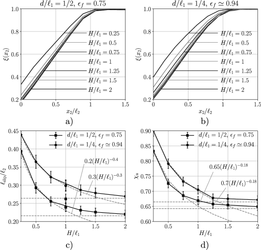
Figure 9: (a,b) Shape $\xi$ of the developed macro-scale velocity profile in the side-wall region of a channel with an array of equidistant square in-line cylinders. The velocity profile $\xi$ is shown for different ratios of the channel height $H$ to the cylinder spacing $\ell_{1}=\ell_{2}$, as well as for different porosities $\epsilon_{f}$. Also the corresponding slip length $\ell_{\text{slip}}$ (c) and displacement factor $\chi_{u}$ (d) for the flow rate in the side-wall region are shown.

The velocity profile $\xi$, and therefore the permeability tensor in the side-wall region, merely depend on the ratio of the channel height $H$ to the cylinder spacing $\ell_{1}=\ell_{2}$ for a fixed porosity $\epsilon_{f}$. The relationship between $\xi$ and $H/\ell_{2}$ is shown in figure 9 (a,b) for two porosities, $\epsilon_{f}=0.75$ and $\epsilon_{f}\simeq 0.94$. According to this figure, the profile $\xi(x_{2})$ becomes almost linear in $x_{2}$ when the channel height is equal to or greater than the cylinder spacing. Still, its first derivative $d\xi/dx_{2}$ is not exactly a constant. In particular in the neighbourhood of the core region, $x_{2}/\ell_{2}\simeq 1$, the first derivative exhibits a discontinuity, indicating a jump in the macro-scale stress $\mu_{f}d\langle u_{1}\rangle_{m}/dx_{2}$ at that location. At the side wall, the first derivative indicates the slip length: $\left.d\xi/dx_{2}\right|_{x_{2}=0}=1/(\ell_{2}+\ell_{\text{slip}})$.

The dependence of the slip length $\ell_{\text{slip}}$ on the ratio of the channel height to cylinder spacing $H/\ell_{2}$ is shown in more detail in figure 9 (c). Just like the velocity profile $\xi$, the slip length clearly becomes independent of the channel height, when the channel height is much larger than the cylinder spacing. This happens due to the fact that when the cylinders are relatively long, so $H/\ell_{2}\gg 1$, the flow patterns around each cylinder are no longer affected by the plate surfaces, nor the distance $H$ between them.

This explains why also the displacement factor $\chi_{u}$ for the flow rate in the side-wall region becomes independent of $H/\ell_{2}$ for $H/\ell_{2}\gg 1$, as shown in figure 9 (d). The latter is defined as the ratio of the mass flow rate through the side-wall region to the mass flow rate through the core region, multiplied with the ratio of the cross-sectional area of the core region to that of the side-wall region. Therefore, it allows us to calculate the magnitude of the uniform macro-scale velocity in the core of the channel, from the bulk velocity:

$$U=\frac{N_{2}}{N_{2}-2N_{\text{sides}}(1-\chi_{u})}u_{b}\,,$$ (43)

if we accept that $\ell_{\text{sides}}$ is a multiple of the unit cell width $\ell_{2}$, so that $N_{\text{sides}}\triangleq 1+\lfloor\ell_{\text{sides}}/\ell_{2}\rfloor$. We remark that the factor $2N_{\text{sides}}$ in (43) corresponds to the number of cylinders in a row parallel to the axis $x_{2}$, located in the region $\Omega_{\text{dev}}\setminus\Omega_{\text{uniform}}$.

The displacement factor $\chi_{u}$ can be seen to correlate well with the slip length $\ell_{\text{slip}}$, if we compare figure 9 (c) and (d). For smaller channel heights, they both obey an empirical power-law scaling with the ratio of the channel height to cylinder spacing, although their exponents differ for the same porosity. Under a few assumptions, their mutual relationship can be made explicit. The first assumption is that $N_{\text{sides}}=1$ so that $\chi_{u}=\left.\langle u_{1}\rangle\right|_{x_{2}=\ell_{\text{sides}}/2}/U$, which is commonly the case as $\ell_{\text{sides}}\simeq\ell_{2}$. The second assumption is that the macro-scale velocity has a linear profile $\xi$ and closely matches the volume-averaged velocity in the side-wall region: $\langle u_{1}\rangle_{m}\simeq\langle u_{1}\rangle$. Then, we have $\chi_{u}\simeq(\ell_{\text{sides}}/2+\ell_{\text{slip}})/(\ell_{\text{sides}}+\ell_{\text{slip}})=\left.\xi\right|_{x_{2}=\ell_{\text{sides}}/2}$. However, this approximation for $\chi_{u}$ has a typical accuracy of around $20\%$ for the data in figure 9 (d), because it is only holds when a single volume-averaging operator is used.

Before we close our discussion on the local closure for the developed region $\Omega_{\text{dev}}$, we emphasize that the permeability tensor $\boldsymbol{K}_{\text{dev}}$ accounts for nearly all macro-scale momentum transport due to gradients of the macro-scale velocity field. So, the momentum equation in $\Omega_{\text{dev}}$ reduces to $\boldsymbol{\nabla}\langle p\rangle^{f}_{m}\simeq\mu_{f}\boldsymbol{K}_{\text{dev}}^{-1}\boldsymbol{\cdot}\boldsymbol{U}^{\prime}_{\text{dev}}$, even though its exact form is $\boldsymbol{\nabla}\langle p\rangle_{m}=\mu_{f}d^{2}U_{\text{dev}}/dx_{2}^{2}\boldsymbol{e}_{1}-\rho_{f}d\langle u_{2}\boldsymbol{u}\rangle_{m}/dx_{2}+\boldsymbol{b}$. The reason is that based on the estimates $x_{2}\sim\ell_{\text{sides}}$ and $U_{\text{dev}}\sim U\sim u_{b}$, we typically have $\|\langle u_{2}\boldsymbol{u}\rangle_{m}\|/u_{b}^{2}\ll 1$ for laminar channel flows, so that the Brinkmann term $\mu_{f}d^{2}U_{\text{dev}}/dx_{2}^{2}$ and the momentum dispersion in the side-wall region are usually negligible at moderate Reynolds numbers $\rho u_{b}\ell_{\text{sides}}/\mu_{f}=\mbox{\it Re}\,(\ell_{\text{sides}}/H)\gg 1$.

6.4 Validity of the Local Closure Problem for Developed Macro-Scale Flow

As Whitaker’s permeability tensor (22) and its extension in the side-wall region (30) are exact once the flow has become periodically developed, the onset point of periodically developed flow, $x_{\text{periodic}}$, is a key parameter to characterize the validity of the preceding local closure models. The scaling laws for $x_{\text{periodic}}$ and their relation to the eigenvalue $\lambda$ in the region of quasi-periodically developed flow, have been discussed in (Buckinx (2022)). Still, the macro-scale flow can often be treated as developed even upstream of the point $x_{\text{periodic}}$.

For instance, if $x_{\text{dev}}$ would have been defined as the $x_{1}$-section in $\Omega_{\text{predev}}$ for which $\|\langle\boldsymbol{u}\rangle_{m}\|=0.99\|\boldsymbol{U}_{\text{dev}}\|$ at $x_{2}=W/2$, we would have found that $x_{\text{dev}}/\ell_{1}\simeq 0.15\mbox{\it Re}+4$ for $\mbox{\it Re}\in(50,300)$ for the flow depicted in figure 3 (a). In that case, we thus have that $x_{\text{dev}}\simeq 0.9x_{\text{periodic}}$, according to the definition of $x_{\text{periodic}}$ adopted in (Buckinx (2022)). Similarly, also for the flow depicted in figure 3 (b), we then would have found that $x_{\text{dev}}/\ell_{1}\simeq 0.19\mbox{\it Re}+4.7$ for $\mbox{\it Re}\in(50,300)$, which is about $10\%$ smaller than $x_{\text{periodic}}/\ell_{1}$ in that case (Buckinx (2022)).

The approximation $\langle\boldsymbol{u}\rangle_{m}\simeq\boldsymbol{U}_{\text{dev}}(\boldsymbol{x})$ is thus accurate even upstream of the periodically developed flow region, $\Omega_{\text{periodic}}$, as it can be seen from figure 2. Therefore, the distinction between $\Omega_{\text{periodic}}$ and $\Omega_{\text{dev}}$ is rather a subtlety from a macro-scale point of view. As a matter of fact, also the distinction between $\Omega_{\text{periodic}}\setminus\Omega_{\text{sides}}$ and $\Omega_{\text{uniform}}$ appears to be a theoretical subtlety, as the approximation $\langle\boldsymbol{u}\rangle_{m}(\boldsymbol{x})\simeq\boldsymbol{U}$ holds well for $\boldsymbol{x}\in(\Omega_{\text{periodic}}\setminus\Omega_{\text{sides}})$. The explanation for these observations is two-fold. Firstly, gradients of the macro-scale velocity in regions like $x_{2}\in(\ell_{\text{sides}},\ell_{\text{sides}}+n_{2}\ell_{2})$ or $x_{1}\in(x_{\text{periodic}},x_{\text{periodic}}+n_{1}\ell_{1})$ occur over a spatial distance smaller than the filter radius and thus tend to be rather small. Secondly, the distance from the side walls at which the flow displays transversal flow periodicity, $\ell_{\text{sides}}$, has been found to be smaller than the transversal spacing of the cylinders, $\ell_{2}$, for all the flow conditions investigated in (Buckinx (2022)).

7 Local Closure for Quasi-Developed Macro-Scale Flow

7.1 Exact Local Closure for Quasi-Developed Macro-Scale Flow

In the region of quasi-periodically developed flow, $\Omega_{\text{quasi-periodic}}$, the quasi-developed closure force is given by

$$\boldsymbol{b}_{\text{quasi-dev}}\simeq\boldsymbol{b}_{\text{dev}}+\langle\boldsymbol{n}_{0}\boldsymbol{\cdot}\left(-\mathsf{P}_{f}\boldsymbol{I}+\mu_{f}\boldsymbol{\nabla}\boldsymbol{\mathsf{U}}_{f}\right)\delta_{0}\rangle_{m}\exp\left(-\boldsymbol{\lambda}\boldsymbol{\cdot}\boldsymbol{x}\right)\,,$$ (44)

as it follows from (4) after substitution of (12) and (14). Again, the approximation symbol in (44) can be replaced by an equality sign, when a matched filter instead of a double-volume averaging operator is chosen.

Also in $\Omega_{\text{quasi-periodic}}$ there exists an apparent permeability tensor $\boldsymbol{K}_{\text{quasi-dev}}\left(\langle\boldsymbol{u}\rangle_{m},\boldsymbol{x}\right)$ to represent the closure force:

$$\boldsymbol{b}_{\text{quasi-dev}}\simeq\langle p\rangle^{f}_{m}\boldsymbol{\nabla}\epsilon_{fm}-\mu_{f}\boldsymbol{K}_{\text{quasi-dev}}^{-1}\boldsymbol{\cdot}\langle\boldsymbol{u}\rangle_{m}\,,$$ (45)

where the quasi-developed macro-scale pressure field in (45) is given by (18). The apparent permeability tensor for quasi-developed macro-scale flow, $\boldsymbol{K}_{\text{quasi-dev}}$, is spatially dependent, but exact in the case of a matched filter, in the sense that for a matched filter, expressions (45) and (18) are no longer approximations.

In order to determine the structure of the tensor $\boldsymbol{K}_{\text{quasi-dev}}$, we introduce a closure mapping which maps the uniform macro-scale velocity in $\Omega_{\text{uniform}}$ to the amplitudes of the velocity and pressure modes in $\Omega_{\text{quasi-periodic}}$:

$$\boldsymbol{\mathsf{U}}(\boldsymbol{r})=\boldsymbol{\Psi}(\boldsymbol{r})\boldsymbol{\cdot}\boldsymbol{U}^{\prime}\qquad\mbox{and}\qquad\mathsf{P}(\boldsymbol{r})=\mu_{f}\boldsymbol{\psi}(\boldsymbol{r})\boldsymbol{\cdot}\boldsymbol{U}^{\prime}\,,$$ (46)

This mapping exists, as we have shown that both $\boldsymbol{\mathsf{U}}$ and $\mathsf{P}$ can be reconstructed from $\boldsymbol{U}^{\prime}$ from the flow equations on one or two rows of the array, when the flow is quasi-periodically developed (Buckinx (2022)). The mapping gives rise to a closure problem for the closure variables $\boldsymbol{\Psi}$ and $\boldsymbol{\psi}$ which is included in appendix C. This closure problem can still be considered a local closure problem, although it has to be solved on a transversal row of the array, instead of a single unit cell. Furthermore, it defines the transformation $\boldsymbol{\zeta}$ from $\boldsymbol{U}^{\prime}$ to $\langle\boldsymbol{\mathsf{U}}\rangle^{f}_{m}$:

$$\langle\boldsymbol{\mathsf{U}}\rangle^{f}_{m}(x_{2})=\boldsymbol{\zeta}(\boldsymbol{U},x_{2})\boldsymbol{\cdot}\boldsymbol{U}^{\prime}\qquad\mbox{with}\qquad\boldsymbol{\zeta}\triangleq\langle\boldsymbol{\Psi}\rangle^{f}_{m}\,,$$ (47)

as well as the mapping from $\langle\boldsymbol{\mathsf{U}}\rangle^{f}_{m}$ to $\langle\boldsymbol{u}\rangle^{f}_{m}$:

$$\langle\boldsymbol{u}\rangle^{f}_{m}(\boldsymbol{x})=\left[\boldsymbol{\xi}(\boldsymbol{U},x_{2})+\boldsymbol{\zeta}(\boldsymbol{U},x_{2})\exp\left(-\boldsymbol{\lambda}\boldsymbol{\cdot}\boldsymbol{x}\right)\right]\boldsymbol{\cdot}\boldsymbol{U}^{\prime}\,,$$ (48)

by virtue of (16) and (31).

After substitution of the closure mapping (46), we find that the last term of (44) can be represented as

$$\langle\boldsymbol{n}_{0}\boldsymbol{\cdot}\left(-\mathsf{P}_{f}\boldsymbol{I}+\mu_{f}\boldsymbol{\nabla}\boldsymbol{\mathsf{U}}_{f}\right)\delta_{0}\rangle_{m}=-\mu_{f}\boldsymbol{\mathsf{K}}^{-1}\boldsymbol{\cdot}\langle\boldsymbol{\mathsf{U}}\rangle_{m}\,,$$ (49)

where the tensor $\boldsymbol{\mathsf{K}}$ is defined by

$$\boldsymbol{\mathsf{K}}^{-1}\triangleq\epsilon_{fm}^{-1}\langle\boldsymbol{n}_{0}\boldsymbol{\cdot}\left(\boldsymbol{I}\boldsymbol{\psi}_{f}-\boldsymbol{\nabla}\boldsymbol{\Psi}_{f}\right)\delta_{0}\rangle_{m}\boldsymbol{\cdot}\boldsymbol{\zeta}^{-1}\,.$$ (50)

This result implies that the apparent permeability tensor from (45) is given by

$$\boldsymbol{K}_{\text{quasi-dev}}^{-1}\triangleq\left[\boldsymbol{K}_{\text{dev}}^{-1}\boldsymbol{\cdot}\boldsymbol{\xi}+\boldsymbol{\mathsf{K}}^{-1}\boldsymbol{\cdot}\boldsymbol{\zeta}\exp\left(-\boldsymbol{\lambda}\boldsymbol{\cdot}\boldsymbol{x}\right)\right]\boldsymbol{\cdot}\left[\boldsymbol{\xi}+\boldsymbol{\zeta}\exp\left(-\boldsymbol{\lambda}\boldsymbol{\cdot}\boldsymbol{x}\right)\right]^{-1}\,,$$ (51)

as one can verify from (44) and (30). We thus conclude that the apparent permeability tensor for quasi-developed macro-scale flow, $\boldsymbol{K}_{\text{quasi-dev}}$, consists of two contributions. On the one hand, it contains a contribution from the apparent permeability tensor for developed macro-scale flow, $\boldsymbol{K}_{\text{dev}}$. This contribution becomes equal to the apparent permeability tensor for uniform macro-scale flow, outside of the side-wall region: $\boldsymbol{K}_{\text{dev}}^{-1}\boldsymbol{\cdot}\boldsymbol{\xi}=\boldsymbol{K}_{\text{uniform}}^{-1}$. On the other hand, it contains a contribution from the permeability tensor $\boldsymbol{\mathsf{K}}$, which expresses the resistance against the macro-scale velocity mode $\langle\boldsymbol{\mathsf{U}}\rangle_{m}$ that occurs on top of the developed macro-scale flow, as long as the flow is still developing. Since both contributions can be determined from the continuity and momentum equations for quasi-periodically developed flow on a transversal row of the array, so can the apparent permeability tensor for quasi-developed macro-scale flow. However, while both contributions vary only along the coordinate $x_{2}$ in the transversal direction, the apparent permeability tensor for quasi-developed macro-scale flow also varies along the main flow direction $x_{1}$. In particular, $\boldsymbol{K}_{\text{quasi-dev}}$ decays exponentially in the main flow direction at a rate imposed by the eigenvalue $\lambda$.

Finally, we have deduced that $\boldsymbol{K}_{\text{quasi-dev}}$ is affected by the tensor $\boldsymbol{\zeta}$, whose magnitude indicates the relative magnitude of the macro-scale velocity mode, as $\|\boldsymbol{\zeta}\boldsymbol{\cdot}\boldsymbol{e}_{1}\|=\|\langle\boldsymbol{\mathsf{U}}\rangle^{f}_{m}\|/U^{\prime}$ according to (47). So, $\boldsymbol{K}_{\text{quasi-dev}}$ is affected by the scaling factor $C_{\boldsymbol{\mathsf{U}}}/U^{\prime}$, which expresses how strong the quasi-developed macro-scale flow is perturbed from the uniform developed macro-scale flow. To make this dependency more explicit, we may write $\boldsymbol{\zeta}=\boldsymbol{\zeta}_{\text{ref}}\,C_{\boldsymbol{\mathsf{U}}}/U^{\prime}$, such that $\boldsymbol{\zeta}_{\text{ref}}\boldsymbol{\cdot}\boldsymbol{e}_{1}=\langle\boldsymbol{\mathsf{U}}\rangle^{f}_{m}/C_{\boldsymbol{\mathsf{U}}}$. In that case, we have $\boldsymbol{e}_{1}\boldsymbol{\cdot}\langle\boldsymbol{\zeta}_{\text{ref}}\rangle_{\text{row}}\boldsymbol{\cdot}\boldsymbol{e}_{1}=1$ because $C_{\boldsymbol{\mathsf{U}}}\triangleq\langle\boldsymbol{\mathsf{U}}\rangle_{\text{row}}$, which shows that $\boldsymbol{\zeta}_{\text{ref}}$ does not depend on the relative perturbation size $C_{\boldsymbol{\mathsf{U}}}^{+}\triangleq C_{\boldsymbol{\mathsf{U}}}/U^{\prime}$, nor the manner in which the flow develops. Since the perturbation size often tends to be relatively small, i.e. $\boldsymbol{\zeta}\ll\boldsymbol{I}$ as $\|\langle\boldsymbol{\mathsf{U}}\rangle^{f}_{m}\|\ll U^{\prime}$, the following approximation for $\boldsymbol{K}_{\text{quasi-dev}}$ is usually acceptable:

$$\boldsymbol{K}_{\text{quasi-dev}}^{-1}\simeq\boldsymbol{K}_{\text{dev}}^{-1}+C_{\boldsymbol{\mathsf{U}}}^{+}\boldsymbol{\mathsf{K}}^{-1}\boldsymbol{\cdot}\boldsymbol{\zeta}_{\text{ref}}\boldsymbol{\cdot}\boldsymbol{\xi}^{-1}\exp\left(-\boldsymbol{\lambda}\boldsymbol{\cdot}\boldsymbol{x}\right)\,.$$ (52)

The previous expression elucidates that the term $C_{\boldsymbol{\mathsf{U}}}^{+}\boldsymbol{\mathsf{K}}^{-1}\boldsymbol{\cdot}\boldsymbol{\zeta}_{\text{ref}}\boldsymbol{\cdot}\boldsymbol{\xi}^{-1}\exp\left(-\boldsymbol{\lambda}\boldsymbol{\cdot}\boldsymbol{x}\right)$ is an asymptotic correction to the apparent permeability tensor from the classical closure problem for developing flow. This correction term will allow us to analyse the validity of the classical closure problem for quasi-developed macro-scale flow, as well as its closure mapping (see appendix D). Yet, before we present this validity analysis, the underlying assumptions and solutions of the classical closure problem are discussed first, in the next subsection.

7.2 Approximative Local Closure for Quasi-Developed Macro-Scale Flow
Outside the Side-Wall Region

For a first approximation, the closure force in $\Omega_{\text{quasi-periodic}}$, and possibly even $\Omega_{\text{predev}}$, may be modelled according to the classical closure problem of Whitaker (1996). In that case, the closure force $\boldsymbol{b}$ has an approximative local representation of the form

$$\boldsymbol{b}_{\text{approx}}\triangleq-\mu_{f}\boldsymbol{K}^{-1}_{\text{approx}}\left(\langle\boldsymbol{u}\rangle_{m}\right)\boldsymbol{\cdot}\langle\boldsymbol{u}\rangle_{m}\,,$$ (53)

outside the side-wall region $\Omega_{\text{sides}}$, where $\boldsymbol{\nabla}\epsilon_{fm}=0$. The apparent permeability tensor $\boldsymbol{K}_{\text{approx}}$ is defined in terms of the closure variables ${\widetilde{\boldsymbol{\Phi}}}$ and ${\widetilde{\boldsymbol{\varphi}}}$, through the mappings $\widetilde{\boldsymbol{u}}(\boldsymbol{r})={\widetilde{\boldsymbol{\Phi}}}(\boldsymbol{r})\boldsymbol{\cdot}\langle\boldsymbol{u}\rangle^{f}_{m}(\boldsymbol{x})$ and $\widetilde{p}(\boldsymbol{r})={\widetilde{\boldsymbol{\varphi}}}(\boldsymbol{r})\boldsymbol{\cdot}\langle\boldsymbol{u}\rangle^{f}_{m}(\boldsymbol{x})$:

$$\boldsymbol{K}^{-1}_{\text{approx}}\triangleq\epsilon_{fm}^{-1}\langle\boldsymbol{n}_{0}\boldsymbol{\cdot}(\boldsymbol{I}{\widetilde{\boldsymbol{\varphi}}_{f}}-\boldsymbol{\nabla}{\widetilde{\boldsymbol{\Phi}}_{f}})\delta_{0}\rangle_{m}\,.$$ (54)

The classical closure problem itself, which governs an approximative solution for the deviation fields ($\widetilde{\boldsymbol{u}}$, $\widetilde{p}$) and the closure variables (${\widetilde{\boldsymbol{\Phi}}}$, ${\widetilde{\boldsymbol{\varphi}}}$) as a function of $\langle\boldsymbol{u}\rangle_{m}$, is given by

$$\rho_{f}\left(\langle\boldsymbol{u}\rangle^{f}_{m}+\widetilde{\boldsymbol{u}}_{f}\right)\boldsymbol{\cdot}\boldsymbol{\nabla}\widetilde{\boldsymbol{u}}_{f} =-\boldsymbol{\nabla}\widetilde{p}_{f}+\mu_{f}\nabla^{2}\widetilde{\boldsymbol{u}}_{f}-\epsilon_{fm}^{-1}\boldsymbol{b}\,,$$ (55)

$$\boldsymbol{\nabla}\boldsymbol{\cdot}\widetilde{\boldsymbol{u}}_{f} =0\,,$$ (56)

$$\widetilde{\boldsymbol{u}}_{f}(\boldsymbol{r}) =\widetilde{\boldsymbol{u}}_{f}(\boldsymbol{r}+n_{j}\boldsymbol{l}_{j})\,,\qquad\widetilde{p}_{f}(\boldsymbol{r})=\widetilde{p}_{f}(\boldsymbol{r}+n_{j}\boldsymbol{l}_{j})\,,$$ (57)

$$\widetilde{\boldsymbol{u}} =-\langle\boldsymbol{u}\rangle^{f}_{m}\qquad\mbox{for}~{}~{}\boldsymbol{r}\in\Gamma_{0}\,,$$ (58)

$$\langle\widetilde{\boldsymbol{u}}\rangle_{m} =0\,,$$ (59)

where it is tacitly assumed that $\boldsymbol{r}\in\Omega_{\text{unit}}^{2\times 2}(\boldsymbol{x})$, $j\in\{1,2\}$ and $n_{j}=1$ or $n_{j}=2$.

In order to apply the classical closure problem (55) - (59) to obtain the approximate relationship (53) between $\langle\boldsymbol{u}\rangle_{m}$ and $\boldsymbol{b}$ for developing or quasi-developed macro-scale flow, the following assumptions (or approximations) have to be made, in line with Whitaker’s original derivation. First, the macro-scale momentum dispersion source must be negligible with respect to the closure force, so that only the latter appears in the momentum equation (55):

$$\boldsymbol{b}\gg\rho_{f}\boldsymbol{\nabla}\boldsymbol{\cdot}\boldsymbol{M}\,.$$ (60)

Secondly, the closure force $\boldsymbol{b}$ should depend only on the deviation fields $\widetilde{\boldsymbol{u}}$ and $\widetilde{p}$, or at least, its direct dependence on the macro-scale velocity $\langle\boldsymbol{u}\rangle_{m}$ and pressure $\langle p\rangle_{m}$ should be of minor importance. As shown by Quintard & Whitaker (1994b), for the filter (5) this condition is automatically fulfilled, since in $\Omega_{\text{predev}}\setminus\Omega_{\text{sides}}$, it holds that

$$\boldsymbol{b}=\langle\boldsymbol{n}_{0}\boldsymbol{\cdot}(-\widetilde{p}_{f}\boldsymbol{I}+\mu_{f}\nabla\widetilde{\boldsymbol{u}}_{f})\delta_{0}\rangle_{m}\,.$$ (61)

The reason is that in the part of $\Omega_{\text{predev}}$ where $\boldsymbol{\nabla}\epsilon_{fm}$ is zero, also the gradients of all other spatial moments like $\boldsymbol{\nabla}\boldsymbol{m}$ are zero, due to the properties of the double volume-averaging operator (5).

In the third place, the momentum equation (55) incorporates the assumption that

$$\widetilde{\boldsymbol{u}}_{f}\boldsymbol{\cdot}\boldsymbol{\nabla}\widetilde{\boldsymbol{u}}_{f}\gg\widetilde{\boldsymbol{u}}_{f}\boldsymbol{\cdot}\boldsymbol{\nabla}\langle\boldsymbol{u}\rangle^{f}_{m}\,.$$ (62)

The last assumption behind this closure problem is the periodicity (57) of the deviation fields in each unit cell $\Omega_{\text{unit}}^{2\times 2}$ outside the side-wall region. Due to the assumed periodicity of the deviation fields, both $\langle\boldsymbol{u}\rangle^{f}_{m}$ and $\boldsymbol{b}$ appear as spatially constant vectors in the classical closure problem, and their spatial variation within the unit cell is neglected:

$$\langle\boldsymbol{u}\rangle^{f}_{m}(\boldsymbol{r})\simeq\langle\boldsymbol{u}\rangle^{f}_{m}(\boldsymbol{x})\qquad\mbox{and}\qquad\boldsymbol{b}(\boldsymbol{r})\simeq\boldsymbol{b}(\boldsymbol{x})\,,$$ (63)

$\forall\boldsymbol{r}\in\Omega_{\text{unit}}^{2\times 2}(\boldsymbol{x})$, if $\Omega_{\text{unit}}^{2\times 2}(\boldsymbol{x})\subset\left(\Omega_{\text{predev}}\setminus\Omega_{\text{sides}}\right)$.

Because of these four approximations, the classical closure problem is mathematically equivalent to the periodically developed flow equations (Buckinx & Baelmans, 2015a):

$$\boldsymbol{K}_{\text{approx}}\left(\langle\boldsymbol{u}\rangle_{m}\right)=\boldsymbol{K}_{\text{uniform}}\left(\langle\boldsymbol{u}\rangle_{m}\right)\,.$$ (64)

It thus yields the exact apparent permeability tensor for $\Omega_{\text{uniform}}$ when $\langle\boldsymbol{u}\rangle_{m}=\boldsymbol{U}$. Yet, it has to be solved for different directions and magnitudes of $\langle\boldsymbol{u}\rangle_{m}$, since the macro-scale velocity in $\Omega_{\text{predev}}$ may vary from point to point, whereas it is uniform in $\Omega_{\text{uniform}}$.

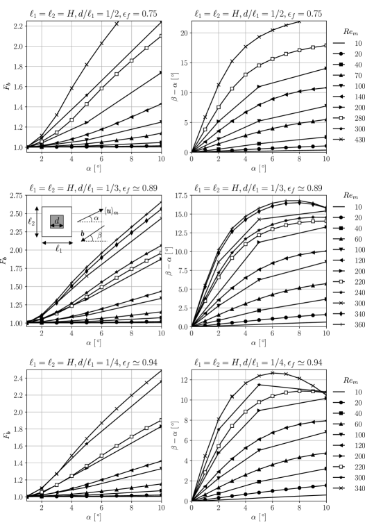
Figure 10: Relative magnitude $F_{\boldsymbol{b}}$ (left) and relative direction $\beta-\alpha$ (right) of the closure force $\boldsymbol{b}$, according to the classical closure problem for an array of equidistant in-line square cylinders. The dependence on the Reynolds number $\mbox{\it Re}_{m}$ and angle of attack $\alpha$ of the macro-scale velocity $\langle\boldsymbol{u}\rangle_{m}$ are shown for different porosities $\epsilon_{f}$, and a fixed height $H=\ell_{1}$.

The numerical solution of the classical closure problem (55) - (59) gives an approximation for the closure force $\boldsymbol{b}(\boldsymbol{x})$ at each point $\boldsymbol{x}\in\left(\Omega_{\text{predev}}\setminus\Omega_{\text{sides}}\right)$, as a function of the local Reynolds number $\mbox{\it Re}_{m}({\boldsymbol{x}})\triangleq 2\rho_{f}\|\langle\boldsymbol{u}\rangle_{m}\|H/\mu_{f}$ based on the local macro-scale velocity $\langle\boldsymbol{u}\rangle_{m}(\boldsymbol{x})$, and the local direction of the macro-scale velocity $\boldsymbol{e}_{s}(\boldsymbol{x})\triangleq\langle\boldsymbol{u}\rangle_{m}/\|\langle\boldsymbol{u}\rangle_{m}\|$. The local direction of the macro-scale velocity is more conveniently represented by the local angle of attack $\alpha\triangleq\arccos\left(\boldsymbol{e}_{1}\boldsymbol{\cdot}\boldsymbol{e}_{s}\right)$, since the macro-scale flow in the channel is two-dimensional.

In figure 10, the dependence of the magnitude and direction of the closure force $\boldsymbol{b}$ on $\mbox{\it Re}_{m}$ and $\alpha$, according to the classical closure problem, is illustrated for an array of equidistant in-line square cylinders. The classical closure problem was solved on a unit cell $\Omega_{\text{unit}}^{1\times 1}$, because the deviation fields $\widetilde{\boldsymbol{u}}$ and $\widetilde{p}$ are known to become periodic for $n_{1}=n_{2}=1$ in the periodically developed flow region. The angle of attack $\alpha$ is shown on the horizontal axis, while different Reynolds numbers $\mbox{\it Re}_{m}$ correspond to different markers, described by the legend for each porosity $\epsilon_{f}$ on the right. On the left side of figure 10, the magnitude $\|\boldsymbol{b}\|$ is expressed by the dimensionless factor $F_{\boldsymbol{b}}(Re_{m},\alpha)$, which is defined by $\|\boldsymbol{b}\|\triangleq F_{\boldsymbol{b}}\|\boldsymbol{b}(U,0)\|$. Here, $\boldsymbol{b}(U,0)$ denotes the closure force found for $\alpha=0$, in the case of a uniform macro-scale velocity $\langle\boldsymbol{u}\rangle_{m}=U\boldsymbol{e}_{1}$ of the same magnitude, as depicted in figure 6. On the right side of figure 10, the direction of the closure force is represented by the angle $\beta\triangleq\pi-\arccos\left(\boldsymbol{e}_{1}\boldsymbol{\cdot}\boldsymbol{b}/\|\boldsymbol{b}\|\right)$.

It is observed that for small angles of attack, $\alpha\in(0,10^{\circ})$, the magnitude of the closure force increases when the angle of attack increases, especially at higher Reynolds numbers. In the selected porosity range $\epsilon_{f}\in(0.75,0.94)$ and for the chosen channel height $H=\ell_{1}=\ell_{2}$, the magnitude of the macro-scale force at an angle $\alpha=10^{\circ}$, is more than twice as large as for aligned flow ($\alpha=0$) with the same speed $U$, if the Reynolds number $\mbox{\it Re}_{m}$ lies above $300$. On the other hand, if the Reynolds number is below $50$, the dependence of the magnitude of the macro-scale force force on the angle of attack is rather small, since for any $\alpha\in(0,10^{\circ})$, the factor $F_{\boldsymbol{b}}$ is below $1.1$.

It can also be seen that the direction of the closure force deviates stronger from the direction of the macro-scale velocity, when the angle of attack or the Reynolds number becomes higher. For instance, at a Reynolds number $\mbox{\it Re}_{m}$ above $100$, the difference in angle between both directions, $\beta-\alpha$, is almost $10^{\circ}$ for $\alpha=10^{\circ}$. However, the difference in direction between the closure force and the macro-scale velocity does not increase monotonically with the angle of attack at a certain Reynolds number. As a matter of fact, a maximum of $\beta-\alpha$ can be identified for each Reynolds number, beyond which the closure force becomes again more parallel to the macro-scale velocity.

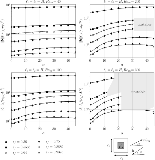
Figure 11: Magnitude of the closure force $\boldsymbol{b}$, according to the classical closure problem for an array of equidistant in-line square cylinders. The dependence on the porosity $\epsilon_{f}$ and angle of attack $\alpha$ is shown for selected Reynolds numbers $\mbox{\it Re}_{m}$, and a fixed height $H=\ell_{1}$. The solid lines ($-$) agree with the correlation (65).

In figure 11, the dependence of the magnitude of the closure force $\boldsymbol{b}$ on the porosity $\epsilon_{f}$ is shown for a wide range of angles of attack $\alpha$, but for selected Reynolds numbers $\mbox{\it Re}_{m}\in\left\{40,100,200,300\right\}$. At the higher Reynolds numbers $\mbox{\it Re}_{m}=200$ and $\mbox{\it Re}_{m}=300$, some of the steady solutions of the classical closure problem obtained for larger angles of attack $\alpha$, were found to correspond to unstable solutions of the (time-dependent) periodically developed flow equations. These unstable solutions have been omitted here, but their parameter range has been indicated by the grey-coloured areas in figure 11.

With a mean relative error of $3.5\%$ and a maximum relative error of $10\%$, all of the data points in figure 10 (as well as figure 11) satisfy the empirical correlation

$$F_{\boldsymbol{b}}=1+A_{0}\frac{\epsilon_{f}^{2}(1-\epsilon_{f})^{2}}{(1-\epsilon_{f})^{2}+A_{1}|\sin(2\alpha)|}\biggl{(}\frac{\sin^{2}(2\alpha)}{\sin^{2}(2\alpha)+A_{2}}\biggr{)}\biggl{(}1+A_{3}\epsilon_{f}^{6}\sqrt{|\cos(2\alpha)|}\biggr{)}\mbox{\it Re}_{m}^{1.2}\,,$$ (65)

with $A_{0}=0.022$, $A_{1}=0.01$, $A_{2}=0.15$ and $A_{3}=0.83$. This correlation has been obtained through a least-square fitting procedure, and reflects that $F_{\boldsymbol{b}}-1\sim\mbox{\it Re}_{m}^{1.2}$ is a good approximation over the investigated range of Reynolds numbers. Further, it is based on the observation that $F_{\boldsymbol{b}}-1\sim|\sin(2\alpha)|$ for porosities $\epsilon_{f}\leq 0.75$. For higher porosities, the latter form has been corrected into $F_{\boldsymbol{b}}-1\sim|\sin(2\alpha)|(1+A_{3}\sqrt{|\cos(2\alpha)|})$. The correlation also shows that $F_{\boldsymbol{b}}-1\sim\alpha^{2}$ for $\alpha\rightarrow 0$, although the numerical uncertainty on this exponent $2$ was found to be quite significant. Lastly, the correlation has been constructed by matching the approximate asymptotes $F_{\boldsymbol{b}}-1\sim\epsilon_{f}^{2}$ for $\epsilon_{f}\rightarrow 0$ and $F_{\boldsymbol{b}}-1\sim(1-\epsilon_{f})^{2}$ for $\epsilon_{f}\rightarrow 1$, whose intersection point depends on the angle of attack via the term $A_{1}|\sin(2\alpha)|$. We remark that if the coefficients $A_{i}$ in the correlation would be optimized for every single porosity value $\epsilon_{f}$, the maximum relative error of the correlation would be less than $6.5\%$ for that porosity value.

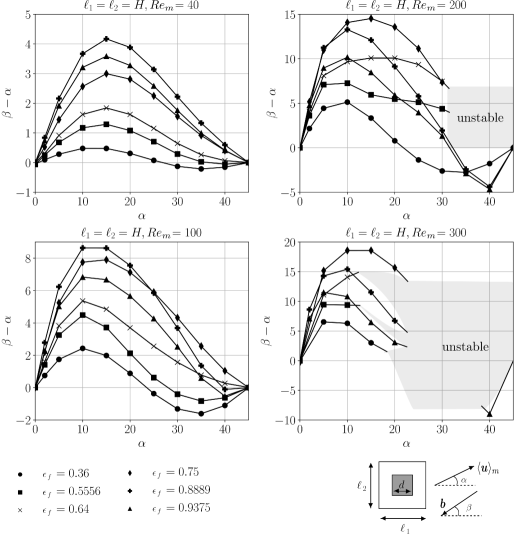
Figure 12: Direction $\beta$ of the closure force $\boldsymbol{b}$, according to the classical closure problem for an array of equidistant in-line square cylinders. The dependence on the porosity $\epsilon_{f}$ and angle of attack $\alpha$ is shown for selected Reynolds numbers $\mbox{\it Re}_{m}$, and a fixed height $H=\ell_{1}$.

The direction $\beta$ of the closure force according to the classical closure problem is given in figure 12. The range of porosities, angles of attack and Reynolds numbers is the same as in the previous figure. The relation between $\beta$ and $\alpha$ is quite complex even for a fixed porosity, especially when the Reynolds number $\mbox{\it Re}_{m}$ is bigger. But for high porosities, it can be described by the correlation

$$\frac{\tan\beta}{\tan\alpha}=1+B_{0}\frac{\mbox{\it Re}_{m}^{2}}{\mbox{\it Re}_{m}+B_{1}}\left(1-|\sin(2\alpha)|\right)\left(1-B_{2}\mbox{\it Re}_{m}^{B_{3}}|\sin(2\alpha)|^{B_{4}}\right)\,.$$ (66)

For a porosity $\epsilon_{f}=0.75$ and angle of attack $\alpha\in(2^{\circ},45^{\circ})$, this correlation captures all of the data points from figures 10 and 12 with a relative accuracy of $4\%$, if $B_{0}=0.040$, $B_{1}=22$, $B_{2}=0.004$, $B_{3}=1$ and $B_{4}=0.5$. For a porosity $\epsilon_{f}\simeq 0.89$, the correlation is accurate to within $6\%$ when $\alpha\in(2^{\circ},35^{\circ})$, if $B_{0}=0.040$, $B_{1}=12$, $B_{2}=0.0075$, $B_{3}=1$ and $B_{4}=0.7$. Moreover, for $\epsilon_{f}\simeq 0.94$ and $\alpha\in(2^{\circ},35^{\circ})$, the correlation is accurate to within $7\%$, if $B_{0}=0.042$, $B_{1}=20$, $B_{2}=0.021$, $B_{3}=0.8$ and $B_{4}=0.5$. On the other hand, for small angles $\alpha\in(0,2^{\circ})$, the relative accuracy of the latter three correlations reduces to $8\%$. The correlation also respects that $\alpha=\beta$ for $\alpha=0^{\circ}$, $\alpha=45^{\circ}$, or $\mbox{\it Re}_{m}\rightarrow 0$.

7.3 Validity of the Classical Closure Problem for Quasi-Developed Flow
Outside the Side-Wall Region – Theoretical Considerations

Although the classical closure problem in $\Omega_{\text{quasi-periodic}}$ has the same mathematical form as the periodically developed flow equations in $\Omega_{\text{uniform}}$, its underlying assumptions (57), (60), (62) and (63) are less restrictive than true flow periodicity. The reason is that these assumptions are also justified under certain length-scale conditions which may hold throughout a wider range of flow regimes, as shown by Whitaker (1996). Therefore, we might expect that already after some section in the region of quasi-periodically developed flow, the local approximation (53) for the actual closure force (44) may become relatively accurate.

In view of this expectation, the question arises how well each of the assumptions behind the classical closure problem is satisfied when the flow is still developing in $\Omega_{\text{quasi-periodic}}$. If we examine the first assumption (57), i.e. the periodicity of the deviation fields of the velocity and pressure in the main flow direction, we find that

$$\widetilde{\boldsymbol{u}}_{f}(\boldsymbol{r}+n_{1}\boldsymbol{l}_{1})-\widetilde{\boldsymbol{u}}_{f}(\boldsymbol{r}) =\widetilde{\boldsymbol{\mathsf{U}}}_{f}(\boldsymbol{r})\exp(-\boldsymbol{\lambda}\boldsymbol{\cdot}\boldsymbol{r})G_{\lambda}\,,$$ (67)

$$\widetilde{p}_{f}(\boldsymbol{r}+n_{1}\boldsymbol{l}_{1})-\widetilde{p}_{f}(\boldsymbol{r}) =\widetilde{\mathsf{P}}_{f}(\boldsymbol{r})\exp(-\boldsymbol{\lambda}\boldsymbol{\cdot}\boldsymbol{r})G_{\lambda}$$ (68)

with $G_{\lambda}\triangleq\exp(-\boldsymbol{\lambda}\boldsymbol{\cdot}n_{1}\boldsymbol{l}_{1})-1$, as a consequence of the defining properties of quasi-periodically developed flow (12)-(15). We thus see that the periodicity conditions for the classical closure problem are violated by the terms on the right hand side of (67) and (68), which are proportional to $C_{\boldsymbol{\mathsf{U}}}\exp(-\boldsymbol{\lambda}\boldsymbol{\cdot}\boldsymbol{r})G_{\lambda}$, since $\widetilde{\boldsymbol{\mathsf{U}}}_{f}\sim C_{\boldsymbol{\mathsf{U}}}$ and $\widetilde{\mathsf{P}}_{f}\sim C_{\boldsymbol{\mathsf{U}}}$.

A similar conclusion is found with respect to the assumption that the variation of the macro-scale velocity and closure force within the unit cell can be ignored (63). Along the main flow direction, we have for instance

$$\langle\boldsymbol{u}\rangle^{f}_{m}(\boldsymbol{r}+n_{1}\boldsymbol{l}_{1})-\langle\boldsymbol{u}\rangle^{f}_{m}(\boldsymbol{r})=\langle\boldsymbol{\mathsf{U}}\rangle^{f}_{m}(\boldsymbol{r})\exp(-\boldsymbol{\lambda}\boldsymbol{\cdot}\boldsymbol{r})G_{\lambda}\,,$$ (69)

by virtue of (16) and (17). In addition, we have

$$\boldsymbol{b}(\boldsymbol{r}+n_{1}\boldsymbol{l}_{1})-\boldsymbol{b}(\boldsymbol{r})=-\mu_{f}\boldsymbol{\mathsf{K}}^{-1}(\boldsymbol{r})\boldsymbol{\cdot}\langle\boldsymbol{\mathsf{U}}\rangle_{m}(\boldsymbol{r})\exp(-\boldsymbol{\lambda}\boldsymbol{\cdot}\boldsymbol{r})G_{\lambda}$$ (70)

due to (49). Hence, the biggest spatial variations of the macro-scale velocity and closure force within the unit cell, which are ignored in the classical closure problem, are also proportional to $C_{\boldsymbol{\mathsf{U}}}\exp(-\boldsymbol{\lambda}\boldsymbol{\cdot}\boldsymbol{r})G_{\lambda}$, as $\langle\boldsymbol{\mathsf{U}}\rangle^{f}_{m}\sim C_{\boldsymbol{\mathsf{U}}}$.

The third assumption, which implies that the gradient of the macro-scale velocity within the unit cell is negligible (62), can be evaluated based on the same criterion as just derived to evaluate the variation of the macro-scale velocity within the unit cell (69). However, in line with (12) and (16), it also requires that

$$-\lambda\langle\boldsymbol{\mathsf{U}}\rangle^{f}_{m}\ll\boldsymbol{e}_{1}\boldsymbol{\cdot}\frac{\partial\widetilde{\boldsymbol{\mathsf{U}}}_{f}}{\partial\boldsymbol{r}}-\lambda\widetilde{\boldsymbol{\mathsf{U}}}_{f}\,.$$ (71)

This condition is expected to be automatically satisfied when $\lambda\ell_{1}\ll 1$, hence as long as the double-volume averaging operator $\langle\;\rangle_{m}$ has the same properties as a matched filter with respect to the mode $\exp(-\boldsymbol{\lambda}\boldsymbol{\cdot}\boldsymbol{r})$. The argument as to why $\lambda\ell_{1}\ll 1$ is a sufficient condition for (71) and thus (62), is that we may estimate $\langle\boldsymbol{\mathsf{U}}\rangle^{f}_{m}$ and $\widetilde{\boldsymbol{\mathsf{U}}}_{f}$ in (71) to have the same order of magnitude, i.e. $O(\langle\boldsymbol{\mathsf{U}}\rangle^{f}_{m})=O(\widetilde{\boldsymbol{\mathsf{U}}}_{f})=O(\boldsymbol{\mathsf{U}}_{f})$, since $\boldsymbol{\mathsf{U}}_{f}(\boldsymbol{x})=0$ for $\boldsymbol{x}\in\Gamma_{0}$, while we have $O(\boldsymbol{r})=O(\ell_{1})$ for $\boldsymbol{r}\in\Omega_{\text{unit}}^{2\times 2}$. As a side note, we add that when $\lambda\ell_{1}\ll 1$, it holds that $G_{\lambda}\simeq-n_{1}\lambda\ell_{1}$.

The last assumption to evaluate is whether the macro-scale momentum dispersion source can be neglected when the flow is quasi-periodically developed, that is (60). The macro-scale momentum dispersion source in $\Omega_{\text{quasi-periodic}}$ is given by

$$\boldsymbol{M} =\boldsymbol{M}^{\star}+\left(\langle\boldsymbol{u}^{\star}\boldsymbol{\mathsf{U}}\rangle_{m}-\langle\boldsymbol{u}^{\star}\rangle^{f}_{m}\langle\boldsymbol{\mathsf{U}}\rangle_{m}+\langle\boldsymbol{\mathsf{U}}\boldsymbol{u}^{\star}\rangle_{m}-\langle\boldsymbol{\mathsf{U}}\rangle^{f}_{m}\langle\boldsymbol{u}^{\star}\rangle_{m}\right)\exp(-\boldsymbol{\lambda}\boldsymbol{\cdot}\boldsymbol{r})$$ (72)

$$\simeq\boldsymbol{M}^{\star}+\left(\langle\widetilde{\boldsymbol{u}}^{\star}\boldsymbol{\mathsf{U}}\rangle_{m}+\langle\boldsymbol{\mathsf{U}}\widetilde{\boldsymbol{u}}^{\star}\rangle_{m}\right)\exp(-\boldsymbol{\lambda}\boldsymbol{\cdot}\boldsymbol{r})$$ (73)

where $\boldsymbol{M}^{\star}\triangleq\langle\boldsymbol{u}^{\star}\boldsymbol{u}^{\star}\rangle_{m}-\langle\boldsymbol{u}^{\star}\rangle^{f}_{m}\langle\boldsymbol{u}^{\star}\rangle_{m}$. Note that (72) has been obtained by neglecting the small advective contributions of the velocity terms which are proportional to $\exp(-2\lambda x_{1})$, since only the mode $\exp(-\lambda x_{1})$ determines the asymptotic convergence of $\boldsymbol{u}$ towards $\boldsymbol{u}^{\star}$ in $\Omega_{\text{quasi-periodic}}$. As $\boldsymbol{M}^{\star}$ is divergence-free outside of $\Omega_{\text{sides}}$, we can deduce that the approximation $\boldsymbol{\nabla}\boldsymbol{\cdot}\boldsymbol{M}\simeq 0$ neglects the contribution of the second term on the right hand side of (72). This contribution is again proportional to $C_{\boldsymbol{\mathsf{U}}}\exp(-\boldsymbol{\lambda}\boldsymbol{\cdot}\boldsymbol{r})$, but it appears to be very small. According to our numerical simulations, the closure term $\rho_{f}\boldsymbol{\nabla}\boldsymbol{\cdot}\boldsymbol{M}$ is at least an order of magnitude smaller than the closure force $\boldsymbol{b}$ over the entire core region of the channel, $\Omega_{\text{core}}$. Moreover, even near the channel inlet and outlet, we have observed that macro-scale momentum dispersion is of minor importance for the boundary conditions studied in this work.

In summary, we conclude that all assumptions behind the classical closure problem are either fulfilled, or violated by an error which is proportional to $C_{\boldsymbol{\mathsf{U}}}\exp(-\boldsymbol{\lambda}\boldsymbol{\cdot}\boldsymbol{r})$ in $\Omega_{\text{quasi-periodic}}$. This explains why the classical closure problem leads to a modelling error for the closure force in $\Omega_{\text{quasi-periodic}}$,

$$\boldsymbol{b}(\boldsymbol{r})-\boldsymbol{b}_{\text{approx}}(\boldsymbol{r})\simeq-\mu_{f}\left[\boldsymbol{\mathsf{K}}^{-1}(\boldsymbol{r})-\boldsymbol{K}^{-1}_{\text{uniform}}\right]\boldsymbol{\cdot}\langle\boldsymbol{\mathsf{U}}\rangle_{m}(\boldsymbol{r})\exp(-\boldsymbol{\lambda}\boldsymbol{\cdot}\boldsymbol{r})\,,$$ (74)

which also scales with $C_{\boldsymbol{\mathsf{U}}}\exp(-\boldsymbol{\lambda}\boldsymbol{\cdot}\boldsymbol{r})$ and thus diminishes in the main flow direction. At least, this is true if the dependence of the permeability tensor $\boldsymbol{K}_{\text{approx}}$ on the macro-scale velocity is sufficiently weak, i.e. when $\boldsymbol{K}_{\text{approx}}\left(\langle\boldsymbol{u}\rangle_{m}\right)\simeq\boldsymbol{K}_{\text{uniform}}\left(\boldsymbol{U}\right)$. This tends to be the case when the Forchheimer coefficient is much smaller than the Darcy coefficient, or when the perturbation size $C_{\boldsymbol{\mathsf{U}}}$ is small.

From the previous analysis, we learn that the classical closure problem will hold with good accuracy over the entire region of quasi-periodically developed flow, under two circumstances. The first circumstance is when the flow develops in such a manner that the relative perturbation size $C_{\boldsymbol{\mathsf{U}}}^{+}\triangleq C_{\boldsymbol{\mathsf{U}}}/U^{\prime}$ is rather small. After all, we see that $\boldsymbol{b}_{\text{approx}}\rightarrow\boldsymbol{b}$ as $C_{\boldsymbol{\mathsf{U}}}\rightarrow 0$, from (74). This circumstance is rather obvious, as it implies that the macro-scale flow can be treated as developed over the entire region of quasi-periodically developed flow. The second circumstance is when the apparent permeability tensors $\boldsymbol{\mathsf{K}}$ and $\boldsymbol{K}_{\text{uniform}}$ match each other closely. In general, however, this will never be exactly the case, because $\boldsymbol{\mathsf{K}}$ and $\boldsymbol{K}_{\text{uniform}}$ are governed by two mathematically very different closure problems. Nevertheless, when the difference between $\boldsymbol{\mathsf{K}}$ and $\boldsymbol{K}_{\text{uniform}}$ is small enough with respect to $C_{\boldsymbol{\mathsf{U}}}^{+}$, the modelling error (74) will be negligible even for larger perturbations. Therefore, it is possible that the classical closure problem yields an accurate approximation for the closure force, not just over the entire region of quasi-periodically developed flow, but even more upstream where the macro-scale flow can be treated as approximately quasi-developed. By this we mean at some point after the section $x_{1}=x_{\text{quasi-dev}}$, with $x_{\text{quasi-dev}}\leq x_{\text{quasi-periodic}}$.

Under other circumstances, the classical closure problem will hold at best over a part of $\Omega_{\text{quasi-periodic}}$. This understanding brings us to the question for which section in $\Omega_{\text{quasi-periodic}}$, or which section after the point $x_{\text{quasi-dev}}$, the relative error between the actual permeability tensor and its approximation from the classical closure problem equals some prescribed value $\varepsilon_{\boldsymbol{K}}$, defined as

$$\varepsilon_{\boldsymbol{K}}\triangleq\|\boldsymbol{I}-\boldsymbol{K}_{\text{approx}}\boldsymbol{\cdot}\boldsymbol{K}^{-1}_{\text{quasi-dev}}\|\,.$$ (75)

Here, $\|\;\|$ denotes an appropriate tensor norm. From (52) and (64) it follows that this section is given by $x_{1}=x_{\text{approx}}$ with

$$x_{\text{approx}}\simeq\frac{1}{\lambda}\ln\left(\frac{\displaystyle\max_{x_{2}\in I_{2}}\|\boldsymbol{K}_{\text{approx}}\boldsymbol{\cdot}\boldsymbol{\mathsf{K}}^{-1}\boldsymbol{\cdot}\boldsymbol{\zeta}_{\text{ref}}\|C_{\boldsymbol{\mathsf{U}}}^{+}}{\varepsilon_{\boldsymbol{K}}}\right)\,,$$ (76)

and $I_{2}\triangleq(\ell_{\text{sides}},W-\ell_{\text{sides}})$. To obtain the last result, it was assumed again that the dependence of the permeability tensor $\boldsymbol{K}_{\text{approx}}$ on the macro-scale velocity is sufficiently weak, so $\boldsymbol{K}_{\text{approx}}\left(\langle\boldsymbol{u}\rangle_{m}\right)\simeq\boldsymbol{K}_{\text{uniform}}\left(\boldsymbol{U}\right)$. Expression (76) reveals that the point where the classical closure problem becomes accurate to within $\varepsilon_{\boldsymbol{K}}$ for some relative perturbation size $C_{\boldsymbol{\mathsf{U}}}^{+}$, satisfies the scaling law

$$x_{\text{approx}}\simeq\frac{1}{\lambda}\left(\ln\frac{C_{\boldsymbol{\mathsf{U}}}^{+}}{\varepsilon_{\boldsymbol{K}}}+c_{3}\right)\,,$$ (77)

with $c_{3}\triangleq\ln\displaystyle\max_{x_{2}\in I_{2}}\|\boldsymbol{K}_{\text{approx}}\boldsymbol{\cdot}\boldsymbol{\mathsf{K}}^{-1}\boldsymbol{\cdot}\boldsymbol{\zeta}_{\text{ref}}\|$, provided that $x_{\text{approx}}\in(x_{\text{quasi-dev}},x_{\text{end}}-n_{1}\ell_{1})$. Of course, this scaling law is only of use once the eigenvalue $\lambda$ and the term $c_{3}$ have been determined by solving the conservation equations for quasi-periodically flow on one or two rows of the array.

We remark that the term $c_{3}$, which is a measure for the difference between $\boldsymbol{\mathsf{K}}$ and $\boldsymbol{K}_{\text{approx}}$, is virtually independent of the macro-scale velocity $\boldsymbol{U}$ and hence the Reynolds number Re, if also the dependence of $\boldsymbol{\mathsf{K}}$ on the macro-scale velocity is weak, next to that of $\boldsymbol{K}_{\text{approx}}$. Therefore, when $c_{3}$ is interpreted as a geometrical property of the channel and its array, the scaling law (77) yields the correct correlation between $x_{\text{approx}}/\ell_{1}$ and Re, as long as the inertial effects on the permeability tensors $\boldsymbol{\mathsf{K}}$ and $\boldsymbol{K}_{\text{approx}}$ (or $\boldsymbol{K}_{\text{uniform}}$) are not too strong. This correlation between $x_{\text{approx}}/\ell_{1}$ and Re tends to be linear, due to the fact that the eigenvalue $\lambda$ scales inversely linear with the Reynolds number in the region of quasi-periodically developed flow (Buckinx (2022)): $x_{\text{approx}}/\ell_{1}\sim 1/(\lambda\ell_{1})\sim c_{1}\mbox{\it Re}+1$. So, at lower Reynolds numbers Re, the apparent permeability tensor according to the classical closure problem, $\boldsymbol{K}_{\text{approx}}$, tends to match $\boldsymbol{K}_{\text{quasi-dev}}$ more upstream towards the channel inlet. Nevertheless, for a given velocity profile at the inlet of the channel, also the relative perturbation size $C_{\boldsymbol{\mathsf{U}}}^{+}$ will change when the Reynolds number Re changes, as the flow will develop differently. In particular, for a parabolic velocity profile at the channel inlet, the relative perturbation size $C_{\boldsymbol{\mathsf{U}}}^{+}$ decreases at higher Reynolds number Re. Yet, the influence of the relative perturbation size $C_{\boldsymbol{\mathsf{U}}}^{+}$ on the point where the classical problem becomes valid, is less pronounced than that on the modelling error (74) itself. The reason is that $x_{\text{approx}}$ does not scale linearly with $C_{\boldsymbol{\mathsf{U}}}^{+}$, but instead scales with its logarithm.

7.4 Validity of the Classical Closure Problem for Quasi-Developed Flow
Outside the Side-Wall Region – Computational Study

Thus far, we have shown that for quasi-developed macro-scale flow, the approximation errors in the classical closure problem, as well as the point where the classical closure problem becomes valid, depend on three factors: the relative perturbation size $C_{\boldsymbol{\mathsf{U}}}^{+}$, which controls the mode amplitudes $\boldsymbol{\mathsf{U}}$ and $\langle\boldsymbol{\mathsf{U}}\rangle_{m}$, the eigenvalue $\lambda$, and lastly the difference between $\boldsymbol{\mathsf{K}}$ and $\boldsymbol{K}_{\text{uniform}}$. So, a complete treatise on the validity of (53) would require first an assessment of the relative perturbation size or magnitude of the mode amplitudes for a large set of relevant inlet conditions and channel geometries. However, the formulation and characterization of physically realistic inlet conditions falls beyond the scope of the present work. To get some idea of how large the mode amplitudes can be for the class of channel flows discussed in section 2, albeit under the idealized case of a parabolic velocity profile at the channel inlet, we refer the reader to our preceding work (Buckinx (2022)). Here, we limit us to a discussion of the computational results for the macro-scale flow fields from figure 3, to support our main theoretical findings. These computational results, which illustrate the accuracy of the classical closure problem as a model for the closure force in the developing flow region, are displayed in the next figures.

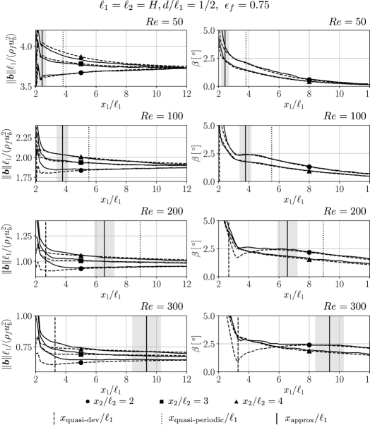
Figure 13: Closure force in the developing flow region of a channel array with a porosity $\epsilon_{f}=0.75$ ($N_{1}=60,N_{2}=10$, $s_{0}/\ell_{1}=1,s_{N}/\ell_{1}=1$, $H/\ell_{1}=1$, $\ell_{1}/\ell_{2}=1$) for different Reynolds numbers Re and different $x_{2}$-sections. The solid lines ($-$) represent the magnitude and angle of the actual closure force $\boldsymbol{b}$. The dashed lines (- -) represent the solution of the classical closure problem, $\boldsymbol{b}_{\text{approx}}$. The onset points of quasi-periodic and quasi-developed flow, $x_{\text{quasi-periodic}}$ and $x_{\text{quasi-dev}}$ have been indicated by a dotted and a dashed vertical line respectively. The solid vertical line marks the point $x_{\text{approx}}$ from where on the classical closure problem is theoretically accurate to within $1\%$.

In figure 13, the solution of the classical closure problem, $\boldsymbol{b}_{\text{approx}}$ from (53), is compared with the actual closure force $\boldsymbol{b}$ in a channel, which consists of an array of $60\times 10$ in-line equidistant square cylinders with a height $H=\ell_{1}=\ell_{2}$ and a porosity $\epsilon_{f}=0.75$. The position of the first and last cylinder row have been chosen as $s_{0}=\ell_{1}$ and $s_{N}=\ell_{1}$.

The actual closure force, whose magnitude $\|\boldsymbol{b}\|$ and direction $\beta$ are given by the solid lines ($-$) in figure 13, has been obtained from a direct numerical simulation of the flow in the channel, for the boundary conditions discussed in section 2. It has been calculated from the closure terms $\boldsymbol{b}_{p}$ and $\boldsymbol{b}_{\tau}$, as defined in section 3, by explicitly filtering the pressure field, the pressure gradient, as well as the viscous stress tensor and its divergence. The latter explicit filtering operation proved to be computationally very demanding, as it required an interpolation of the flow field onto a mesh twice as fine as the one used for the direct numerical simulation of the flow (thus containing up to 250 million mesh cells), in order to keep the average relative discretization error on $\|\boldsymbol{b}\|$ below $5\%$.

The approximation for the closure force according to the classical closure problem, $\boldsymbol{b}_{\text{approx}}$, which is indicated by the dashed lines (- -) in figure 13, has been obtained in three steps. First, the macro-scale velocity in the developing flow region was acquired by explicit filtering of the velocity field, to get the local angle of attack $\alpha$ and local Reynolds number $\mbox{\it Re}_{m}$ at each point of $\Omega_{\text{predev}}$. Then, the closure equations (55) - (59) were solved to construct a data table for $F_{\boldsymbol{b}}$ and $\beta$ for an extensive set of angles of attack and local Reynolds numbers, covering the actual range of $\alpha$ and $\mbox{\it Re}_{m}$ in the developing flow region. That way, the value of $\boldsymbol{b}_{\text{approx}}$ was already obtained for certain points in $\Omega_{\text{predev}}$. Finally, two-dimensional interpolation based on univariate cubic splines and linear radial basis functions was used to evaluate $F_{\boldsymbol{b}}$ and $\beta$ for the intermediate values of $\alpha$ and $\mbox{\it Re}_{m}$ in $\Omega_{\text{predev}}$ that were not included in the data table. The part of the data table for $F_{\boldsymbol{b}}$ and $\beta$ which is most relevant for reproducing the approximation $\boldsymbol{b}_{\text{approx}}$ in figure 13, has been presented earlier in figure 10. Indeed, for all the flow conditions depicted in figure 13, it holds that $\alpha(\boldsymbol{x})\in(0,5^{\circ})$ and $\mbox{\it Re}_{m}(\boldsymbol{x})\in\left(0.4Re,1.3Re\right)$ if $\boldsymbol{x}\in\Omega_{\text{predev}}$, and $\mbox{\it Re}_{m}\simeq 1.07\mbox{\it Re}$ in $\Omega_{\text{uniform}}$. Therefore, a complete overview of the data table used for the interpolation has been omitted here. Besides, the data table is quite extensive, since the classical closure problem was solved numerically for more than 850 different combinations of $\alpha$, $\mbox{\it Re}_{m}$ and $\epsilon_{f}$, to keep the estimated interpolation error below $5\%$ (including the estimated maximum discretization error of $1.5\%$ on the values in the data table itself). Almost 300 different simulations of the classical closure problem were carried out for just the geometry selected in figure 13.

By comparing the actual closure force with its approximation according to the classical closure problem in figure 13, we see that both converge downstream along the main flow direction. As explained before, once the macro-scale velocity and the closure force have become uniform due to the onset of periodically developed flow, both are in exact agreement, apart from a small discretization error, which is in this case around $1\%$. For the channel in figure 13, this exact agreement between $\boldsymbol{b}$ and $\boldsymbol{b}_{\text{approx}}$ occurs around $x_{1}=x_{\text{dev}}$, with $x_{\text{dev}}\simeq 12\ell_{1}$ when $\mbox{\it Re}=50$, and $x_{\text{dev}}\simeq 52\ell_{1}$ when $\mbox{\it Re}=300$.

We also see that over the largest part of the developing flow region, the approximation based on the classical closure problem is already quite accurate. For instance, when $\mbox{\it Re}\leq 100$, the solution of the classical closure problem deviates no more than $5\%$ in magnitude and $10\%$ in angle from the actual closure force, for $x_{1}/\ell_{1}\geq 2.5$. At higher Reynolds numbers, i.e. $200\leq\mbox{\it Re}\leq 300$, the same quantitative agreement is reached more downstream, for $x_{1}/\ell_{1}\geq 6$. If we take into account that the estimated discretization errors for $\|\boldsymbol{b}\|$ and $\beta$ are around $2.5\%$ and $10\%$ respectively (and certainly below $5\%$ and $15\%$), while the numerical solution of the classical closure problem has an estimated error of $1\%$ to $3\%$ (and certainly less than $5\%$) due to the interpolation, we can conclude that the classical closure problem yields an approximation which is accurate to within the margin of numerical uncertainty almost everywhere, except near the inlet region. Close to the inlet region, around $x_{1}/\ell_{1}=2$, the relative difference between the solution of the classical closure problem and the actual closure force, is more than $25\%$ in terms of magnitude and angle, for all Reynolds numbers illustrated.

Despite the quantitatively good agreement between $\boldsymbol{b}_{\text{approx}}$ and $\boldsymbol{b}$ over most of the developing flow region, the difference $\boldsymbol{b}-\boldsymbol{b}_{\text{approx}}$ nowhere becomes zero in $\Omega_{\text{predev}}$: apart from locations with small discretization errors, there is everywhere some distance between the solid and dotted lines in figure 13. We do observe that the difference $\boldsymbol{b}-\boldsymbol{b}_{\text{approx}}$ decreases exponentially in the main flow direction after the section $x_{1}=x_{\text{quasi-dev}}$, as predicted by (74). Inevitably, this exponentially decreasing modelling error arises due to discrepancies between $\boldsymbol{K}_{\text{approx}}$ and $\boldsymbol{\mathsf{K}}$, whose largest components differ by as much as $20\%$, or even $40\%$, depending on the transversal position $x_{2}/\ell_{2}$. These discrepancies between $\boldsymbol{K}_{\text{approx}}$ and $\boldsymbol{\mathsf{K}}$ result in just a minor modelling error $\|\boldsymbol{b}-\boldsymbol{b}_{\text{approx}}\|/\|\boldsymbol{b}\|$ of less than $1\%$ in $\Omega_{\text{quasi-periodic}}$, because the amplitude of the macro-scale velocity mode is rather small: $\|\langle\boldsymbol{\mathsf{U}}\rangle_{m}\|<0.25U$ (see figure 4). Therefore, the local solution of the classical closure problem can barely be distinguished from the actual closure force in $\Omega_{\text{quasi-periodic}}$.

The point $\hat{x}_{\text{approx}}$ from where on the approximation $\boldsymbol{b}_{\text{approx}}$ deviates no more than $1\%$ in magnitude and $10\%$ in angle from the actual closure force $\boldsymbol{b}$ over the entire core of the channel, lies within the grey-coloured areas in figure 13. The width of these grey-coloured areas indicates the numerical uncertainty on the latter point, stemming from the fact that the gradients of $\boldsymbol{b}$ in the direction of the $x_{1}$-axis are so small. Even though the point of agreement $\hat{x}_{\text{approx}}$ is located upstream of the region of quasi-periodically flow, hence to the left of the point $x_{\text{quasi-periodic}}$, it still lies in the region where the macro-scale velocity field can be considered quasi-developed, thus to the right of the point $x_{\text{quasi-dev}}$. Therefore, the point $\hat{x}_{\text{approx}}$ still obeys the theoretical scaling law (77). This scaling law corresponds to the vertical solid line in figure 13, and is given by $x_{\text{approx}}/\ell_{1}\simeq 1/(\lambda\ell_{1})\left(\ln(1+c_{2}/Re)-\ln(\varepsilon_{\boldsymbol{K}})-4\right)$ with $\varepsilon_{\boldsymbol{K}}=0.01$ and $1/(\lambda\ell_{1})\simeq 0.05\mbox{\it Re}+0.8$ (Buckinx (2022)). This follows from the fact that $C_{\boldsymbol{\mathsf{U}}}^{+}\sim(1+c_{2}/\mbox{\it Re})$ with $c_{2}=9.6$, as already appeared from (19).

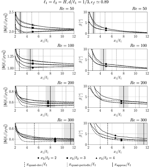
Figure 14: Closure force in the developing flow region of a channel array with a porosity $\epsilon_{f}\simeq 0.89$ ($N_{1}=60,N_{2}=10$, $s_{0}/\ell_{1}=1,s_{N}/\ell_{1}=1$, $H/\ell_{1}=1$, $\ell_{1}/\ell_{2}=1$) for different Reynolds numbers Re and different $x_{2}$-sections. The solid lines ($-$) represent the magnitude and angle of the actual closure force $\boldsymbol{b}$. The dashed lines (- -) represent the solution of the classical closure problem, $\boldsymbol{b}_{\text{approx}}$. The onset points of quasi-periodic and quasi-developed flow, $x_{\text{quasi-periodic}}$ and $x_{\text{quasi-dev}}$ have been indicated by a dotted and a dashed vertical line respectively. The solid vertical line marks the point $x_{\text{approx}}$ from where on the classical closure problem is theoretically accurate to within $1\%$.

In figure 14, another comparison between the actual closure force and its approximation according to the classical closure problem is presented, yet for a channel with a higher porosity $\epsilon_{f}\simeq 0.89$. The actual closure force $\boldsymbol{b}$, indicated by the solid lines ($-$), has again been obtained through direct numerical simulation and explicit filtering of the flow field in the channel. Also the approximation according to the classical closure problem $\boldsymbol{b}_{\text{approx}}$, indicated by the dashed lines (- -), has been determined in a similar fashion as discussed before. In this case, the classical closure problem was solved numerically for more than $250$ combinations of the angle of attack $\alpha$ and local Reynolds number $\mbox{\it Re}_{m}$, with respect to the selected geometry, i.e. $\ell_{1}=\ell_{2}=H$ and $d/\ell_{1}=1/3$. The solutions of the closure problem which are most relevant for reproducing figure 14 have been shown in figure 10, as $\alpha(\boldsymbol{x})\in(0,10^{\circ})$ and $\mbox{\it Re}_{m}(\boldsymbol{x})\in\left(0.5Re,1.3Re\right)$ if $\boldsymbol{x}\in\Omega_{\text{predev}}$, and $\mbox{\it Re}_{m}\simeq 1.07\mbox{\it Re}$ in $\Omega_{\text{uniform}}$.

From the profiles of the actual closure force in figure 14 it can again be seen that in a geometrically similar array with a higher porosity, the onset of the periodically developed flow region is delayed more downstream. The point where the macro-scale flow becomes developed, is now given by $x_{\text{dev}}\simeq 14\ell_{1}$ for $\mbox{\it Re}=50$, while $x_{\text{dev}}\simeq 62\ell_{1}$ for $\mbox{\it Re}=300$, in agreement with the correlation presented in subsection 6.4.

Also in this case, we observe a quantitatively good agreement between the actual closure force $\boldsymbol{b}$ and its approximation $\boldsymbol{b}_{\text{approx}}$ once the macro-scale flow is quasi-developed, despite the fact that the largest components of $\boldsymbol{K}_{\text{approx}}$ and $\boldsymbol{\mathsf{K}}$ differ by as much as $20\%$ or $40\%$ at certain positions. Nevertheless, the difference between $\boldsymbol{b}$ and $\boldsymbol{b}_{\text{approx}}$ in the region of quasi-developed flow is better visible than it was for the porosity $\epsilon_{f}=0.75$. The first reason is that the amplitude of the macro-scale velocity mode is significantly larger, when the flows develops in an array with a higher porosity: $\|\langle\boldsymbol{\mathsf{U}}\rangle_{m}\|<0.35U$ (see figure 4). Secondly, the rate $\lambda$ at which the exponential velocity mode and thus the modelling error (74) vanish after the point $x_{\text{quasi-dev}}$, is smaller: $1/(\lambda\ell_{1})\simeq 0.06\mbox{\it Re}+0.7$ (Buckinx (2022)).

For the same two reasons, the section after which the classical closure problem is theoretically accurate within a relative error $\varepsilon_{\boldsymbol{K}}=0.01$, is located more downstream: $x_{\text{approx}}/\ell_{1}\simeq 1/(\lambda\ell_{1})\left(\ln(1+c_{2}/Re)-\ln(\varepsilon_{\boldsymbol{K}})-4\right)$, where $c_{2}=13$. The position of the latter section, $x_{\text{approx}}$, could not be calculated without numerical uncertainty from the data itself in figure 14, because the relative discretization error for the angle $\beta$ is around $10\%$ when $\mbox{\it Re}\leq 100$, and may become as large as $50\%$ when $\mbox{\it Re}\geq 200$. Such a high upper bound for the discretization error on $\beta$ is attributed to the fact that in a high-porosity array, the macro-scale flow field will have almost no transversal component at higher Reynolds numbers: $\beta\simeq\alpha\simeq\langle{\mathsf{U}_{2}}\rangle_{m}/U_{\text{dev}}\exp(\lambda x_{1})\simeq 0$, as $\langle{\mathsf{U}_{2}}\rangle_{m}/U_{\text{dev}}\sim\lambda(1+c_{2}/\mbox{\it Re})\sim 1/\mbox{\it Re}$ for sufficiently high Re. On the other hand, the discretization error for the magnitude $\|\boldsymbol{b}\|$ is comparable to that in figure 13. Therefore, the closest numerical approximation for $x_{\text{approx}}$, denoted by $\hat{x}_{\text{approx}}$, has been indicated instead in figure 14, by means of the grey areas, just like in the previous figure. This position $\hat{x}_{\text{approx}}$ from where on $\boldsymbol{b}_{\text{approx}}$ deviates no more than $1\%$ in magnitude and $10\%$ in angle from $\boldsymbol{b}$ can be seen to obey the theoretical scaling law derived for $x_{\text{approx}}$.

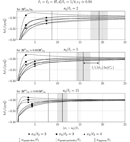
Figure 15: Closure force in the developing flow region of a channel array with a porosity $\epsilon_{f}\simeq 0.94$ ($N_{1}=90,N_{2}=10$, $s_{N}/\ell_{1}=1$, $H/\ell_{1}=1$, $\ell_{1}/\ell_{2}=1$) for different Reynolds numbers Re, different positions of the first cylinder row $s_{0}$, and different $x_{2}$-sections. The solid lines ($-$) represent the component $b_{1}$ of the actual closure force along the main flow direction. The dashed lines (- -) represent the solution of the classical closure problem, $b_{\text{approx},1}$. The onset points of quasi-periodic and quasi-developed flow, $x_{\text{quasi-periodic}}$ and $x_{\text{quasi-dev}}$ have been indicated by a dotted and a dashed vertical line respectively. The solid vertical line marks the point $x_{\text{approx}}$ from where on the classical closure problem is theoretically accurate to within $1\%$.

The previous figures 13 and 14 confirm our initial expectation that especially in high-porosity arrays at higher Reynolds numbers ($\mbox{\it Re}>100$), the classical closure problem fails to capture the macro-scale features of the developing flow. However, in these figures, the relative perturbation size and thus the mode amplitudes were altered by each change in Reynolds number, as the dimensionless velocity profile $\boldsymbol{u}/u_{b}$ at the channel inlet was kept fixed. As a consequence, we observed a smaller mode amplitude at higher Reynolds numbers, which is a favourable condition with regard to the accuracy of the classical closure problem, even though it is outdone by the accompanying decrease of the eigenvalue $\lambda$. It is therefore instructive to inspect the isolated effect of different mode amplitudes at a fixed (high) Reynolds number, as illustrated in figure 15 for an array with an even higher porosity $\epsilon_{f}\simeq 0.94$.

In figure 15, the closure force $\boldsymbol{b}$ and its approximation $\boldsymbol{b}_{\text{approx}}$ are shown for each of the three mode amplitudes $\langle\boldsymbol{\mathsf{U}}^{\prime}\rangle_{m}$, $\langle\boldsymbol{\mathsf{U}}^{\prime\prime}\rangle_{m}$ and $\langle\boldsymbol{\mathsf{U}}^{\prime\prime\prime}\rangle_{m}$ depicted in figure 3 (c). These three mode amplitudes, which all have the same shape but a different magnitude, have thus been obtained by varying the distance $s_{0}$ between the inlet and the first cylinder row, so that at the beginning of the array, at $x_{1}=s_{0}$, a different velocity profile was achieved. Only the component $b_{1}$ along the main flow direction $x_{1}$ is shown in figure 15, because the transversal component $b_{2}$ is so small that its numerical values suffer from significant discretization errors. We remark that the Reynolds number Re, which equals $300$ in this case, should be considered as high for a steady laminar flow, because it is quite close to the critical Reynolds number at which chaotic vortex shedding starts to occur in the selected channel and array geometry. In fact, the critical Reynolds number lies somewhere between $320$ and $400$ according to our direct numerical simulations.

The grey-coloured areas in figure 15 indicate this time the location of the point $\hat{x}_{\text{approx}}$ from where on the approximation $b_{\text{approx,1}}$ deviates no more than $2\%$ in magnitude from the actual closure force $b_{1}$ over the entire cross section of the channel. As before, their width reflects the numerical uncertainty on $\hat{x}_{\text{approx}}$ due to the flatness of the $b_{1}$-curves. The location of the grey-coloured areas is well predicted by the theoretical scaling law for $x_{\text{approx}}$ (77), provided that we take $\varepsilon_{\boldsymbol{K}}=0.01$ instead of $\varepsilon_{\boldsymbol{K}}=0.02$. This numerical inconsistency for $\varepsilon_{\boldsymbol{K}}$ is caused by two factors. On the one hand, the estimated discretization error for $b_{1}$ lies between $1\%$ and $4\%$. On the other hand, also the underlying assumption that $\boldsymbol{K}_{\text{approx}}\left(\langle\boldsymbol{u}\rangle_{m}\right)\simeq\boldsymbol{K}_{\text{uniform}}\left(\boldsymbol{U}\right)$ leads to an error on $b_{1}$ of at least $2\%$, as inertia effects are more important at at the current Reynolds number and porosity.

Notwithstanding this small inconsistency, we clearly notice in figure 15 that both points $\hat{x}_{\text{approx}}$ and $x_{\text{approx}}$ shift upstream over a distance $1/\lambda\ln C_{r}$, upon a reduction of the relative perturbation size by a factor $C_{r}\triangleq\langle{\mathsf{U}_{1}}^{\prime}\rangle_{m}/\langle{\mathsf{U}_{1}}^{\prime\prime}\rangle_{m}$, from the larger mode $\langle\boldsymbol{\mathsf{U}}^{\prime}\rangle_{m}$ to the smaller one, $\langle\boldsymbol{\mathsf{U}}^{\prime\prime}\rangle_{m}$. Due to this shift, the points $\hat{x}_{\text{approx}}$ and $x_{\text{approx}}$ for the mode $\langle\boldsymbol{\mathsf{U}}^{\prime\prime}\rangle_{m}$ end up much closer to the onset point of quasi-periodically developed flow, $x_{\text{quasi-periodic}}$. We also notice that a further decrease of the relative perturbation size, causing the mode amplitude to change from $\langle\boldsymbol{\mathsf{U}}\rangle_{m}$ to $\langle\boldsymbol{\mathsf{U}}^{\prime\prime\prime}\rangle_{m}$, eventually moves the points $\hat{x}_{\text{approx}}$ and $x_{\text{approx}}$ further downstream to the point $x_{\text{quasi-dev}}$, from where on the macro-scale flow can be treated as quasi-developed. These findings illustrate that Whitaker’s permeability tensor $\boldsymbol{K}_{\text{uniform}}$ suffices to accurately describe quasi-developed flow, even at at higher Reynolds numbers and higher porosities, as long as the mode amplitude is small enough. However, for larger mode amplitudes like $\langle\boldsymbol{\mathsf{U}}^{\prime}\rangle_{m}$, only the exact permeability tensor $\boldsymbol{K}_{\text{quasi-dev}}$ will accurately describe the macro-scale flow from the point $x_{\text{quasi-dev}}$ onwards. How large the mode amplitude $\langle\boldsymbol{\mathsf{U}}\rangle_{m}$ needs to be before the exact permeability tensor $\boldsymbol{K}_{\text{quasi-dev}}$ becomes of practical interest, depends on the tensor $\boldsymbol{\mathsf{K}}$, as it is the mode amplitude of the closure force, $\mu_{f}\boldsymbol{\mathsf{K}}^{-1}\boldsymbol{\cdot}\langle\boldsymbol{\mathsf{U}}\rangle_{m}$, which dictates the error of using $\boldsymbol{K}_{\text{uniform}}$ instead of $\boldsymbol{K}_{\text{quasi-dev}}$. So, a relatively large mode amplitude $\langle\boldsymbol{\mathsf{U}}\rangle_{m}$ does not necessarily imply a large error when replacing $\boldsymbol{K}_{\text{quasi-dev}}$ by $\boldsymbol{K}_{\text{uniform}}$. For instance, in figure 15, the relative size of the mode amplitude of the closure force, $\mu_{f}\|\boldsymbol{\mathsf{K}}^{-1}\boldsymbol{\cdot}\langle\boldsymbol{\mathsf{U}}\rangle_{m}\|/\|\boldsymbol{b}^{\star}\|$, is about a factor four smaller than $\langle\boldsymbol{\mathsf{U}}\rangle_{m}/U$. Vice versa, a small change in mode amplitude of the closure force can have a notable impact on the resulting mode amplitude of the macro-scale velocity field.

7.5 Validity of the Classical Closure Problem for Quasi-Developed Flow
Inside the Side-Wall Region

In the side-wall region $\Omega_{\text{sides}}$, the classical closure problem tends to yield a very poor approximation of the actual closure force, due to the strong gradients of the (macro-scale) velocity field that form perpendicular to the side walls, as the flow is slowed down by viscous stresses near the solid boundaries. However, the closure problem for developed macro-scale flow presented in section 6.2, which is an extension of the classical closure problem over $\Omega_{\text{sides}}$, can hold well enough to use the approximation $\boldsymbol{b}_{\text{approx}}=\langle p\rangle^{f}_{m}\boldsymbol{\nabla}\epsilon_{fm}-\mu_{f}\boldsymbol{K}_{\text{dev}}^{-1}(\langle\boldsymbol{u}\rangle_{m})\boldsymbol{\cdot}\langle\boldsymbol{u}\rangle_{m}$ for quasi-developed flow in and outside the side-wall region. The precondition is again that the relative perturbation size $C_{\boldsymbol{\mathsf{U}}}^{+}$ and thus the amplitude of the macro-scale velocity mode are sufficiently small, and that $\boldsymbol{K}_{\text{dev}}(\langle\boldsymbol{u}\rangle_{m})\simeq\boldsymbol{K}_{\text{quasi-dev}}(\boldsymbol{U})$, as it follows from (52).

The point $x^{\prime}_{\text{approx}}$ from where on the latter approximation holds with a relative accuracy $\varepsilon^{\prime}_{\boldsymbol{K}}\triangleq\|\boldsymbol{I}-\boldsymbol{K}_{\text{dev}}\boldsymbol{\cdot}\boldsymbol{K}_{\text{quasi-dev}}^{-1}\|$ also obeys the scaling law (77):

$$x^{\prime}_{\text{approx}}\simeq\frac{1}{\lambda}\left(\ln\frac{C_{\boldsymbol{\mathsf{U}}}^{+}}{\varepsilon^{\prime}_{\boldsymbol{K}}}+c^{\prime}_{3}\right)\,,$$ (78)

if we define $c^{\prime}_{3}\triangleq\ln\displaystyle\max_{x_{2}}\|\boldsymbol{K}_{\text{dev}}\boldsymbol{\cdot}\boldsymbol{\mathsf{K}}^{-1}\boldsymbol{\cdot}\boldsymbol{\zeta}_{\text{ref}}\boldsymbol{\cdot}\boldsymbol{\xi}^{-1}\|$. Often, the point $x^{\prime}_{\text{approx}}$ is little affected by the shape of the developed macro-scale velocity profile $\xi$ itself, because $\boldsymbol{K}_{\text{dev}}\simeq\boldsymbol{\xi}\boldsymbol{\cdot}\boldsymbol{K}_{\text{dev, main}}$ (cf. (38)), so that the tensor $\boldsymbol{\xi}$ contained in $\boldsymbol{K}_{\text{dev}}$ almost cancels its inverse in $c_{3}$. Conversely, it is strongly affected by the difference between $\boldsymbol{K}_{\text{dev, main}}$ and $\boldsymbol{\mathsf{K}}$, which can be significantly large in $\Omega_{\text{sides}}$. Essentially, the larger this difference, the more downstream $x^{\prime}_{\text{approx}}$ will lie, closer to the developed flow region. Therefore, the point $x^{\prime}_{\text{approx}}$ will lie downstream of $x_{\text{approx}}$, when the discrepancy between $\boldsymbol{K}_{\text{dev, main}}$ and $\boldsymbol{\mathsf{K}}$ in $\Omega_{\text{sides}}$ exceeds the discrepancy between $\boldsymbol{K}_{\text{approx}}$ and $\boldsymbol{\mathsf{K}}$ in $\Omega_{\text{core}}$. This means that the closure problem for developed macro-scale flow then will become valid in the side-wall region for some criterion $\varepsilon^{\prime}_{\boldsymbol{K}}=\varepsilon_{\boldsymbol{K}}$, after it has become valid in the core region. On the other hand, when the variation of the tensor $\boldsymbol{K}_{\text{dev, main}}$ over the side-wall region is rather small, such that (40) applies, we find that $x^{\prime}_{\text{approx}}\simeq x_{\text{approx}}$, as $c^{\prime}_{3}\simeq c_{3}$. This situation, where the approximation $\boldsymbol{b}\simeq\boldsymbol{b}_{\text{approx}}=\langle p\rangle^{f}_{m}\boldsymbol{\nabla}\epsilon_{fm}-\mu_{f}\boldsymbol{K}_{\text{dev}}^{-1}(\langle\boldsymbol{u}\rangle_{m})\boldsymbol{\cdot}\langle\boldsymbol{u}\rangle_{m}$ with $\boldsymbol{K}_{\text{dev}}\simeq\boldsymbol{\xi}\boldsymbol{\cdot}\boldsymbol{K}_{\text{uniform}}$, has nearly the same relative accuracy in $\Omega_{\text{sides}}$ as in $\Omega_{\text{core}}$ once the macro-scale flow is quasi-developed, occurs in figure 16.

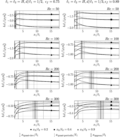
Figure 16: Closure force in the side-wall region of a channel array with a porosity $\epsilon_{f}=0.75$ (left) and $\epsilon_{f}\simeq 0.89$ (right) ($N_{1}=60,N_{2}=10$, $s_{0}/\ell_{1}=1,s_{N}/\ell_{1}=1$, $H/\ell_{1}=1$, $\ell_{1}/\ell_{2}=1$) for different Reynolds numbers Re and different sections $x_{2}/\ell_{2}$. The solid lines ($-$) represent the actual closure force $b_{1}$. The dashed lines (- -) represent the approximate solution of the closure problem for developed macro-scale flow, $b_{\text{approx},1}$, which is based on the permeability tensor $\boldsymbol{K}_{\text{uniform}}$ from the classical closure problem and a linear correlation for $\xi$. The onset points of quasi-periodic and quasi-developed flow, $x_{\text{quasi-periodic}}/\ell_{1}$ and $x_{\text{quasi-dev}}/\ell_{1}$ have been indicated by a dotted and a dashed vertical line respectively. The solid vertical line marks the point $x_{\text{approx}}/\ell_{1}$ from where on the classical closure problem is theoretically accurate to within $1\%$.

In figure 16, the approximation $\boldsymbol{b}_{\text{approx}}$ based on the permeability tensor from the classical closure problem (i.e. based on $\boldsymbol{K}_{\text{dev}}\simeq\boldsymbol{\xi}\boldsymbol{\cdot}\boldsymbol{K}_{\text{uniform}}$), is compared with the actual closure force $\boldsymbol{b}$ in the side-wall region. Only the components $b_{1}$ and $b_{\text{approx},1}$ along the main flow direction are set out, because the transversal component is known a priori for quasi-developed flow: $b_{2}\simeq\langle p\rangle^{f}_{m}d\epsilon_{fm}/dx_{2}$. The different channel flows considered in this figure correspond to two different porosities, $\epsilon_{f}=0.75$ and $\epsilon_{f}\simeq 0.89$. The core regions of these flows have been shown before in figures 13 and 14. It must be remarked that $b_{\text{approx},1}$ is based on the linear approximation for $\xi$ given in (41), instead the exact $\xi$-profile. Therefore, we still observe deviations between $b_{\text{approx},1}$ and $b_{1}$ after the section $x_{1}=x_{\text{approx}}$, even though $x^{\prime}_{\text{approx}}$ is close to $x_{\text{approx}}$ within one to three unit cell lengths $\ell_{1}$ for the exact $\xi$-profile, over the displayed Reynolds number range.

We remark that as the Reynolds number Re increases in figure 16, the local angle of attack $\alpha(\boldsymbol{x})$ in $\Omega_{\text{sides}}$ increases, while it was seen to decrease in $\Omega_{\text{core}}$. This is a consequence of the shape of the mode amplitudes illustrated in figure 4.

8 Reconstruction of Quasi-Developed Macro-Scale Flow

The preceding theoretical considerations and empirical evidence suggest that the closure models for developed flow (30) and quasi-developed flow (45) are not able to capture the flow development before the point $x_{\text{quasi-dev}}$, whether the mode amplitude $\langle\boldsymbol{\mathsf{U}}\rangle_{m}$ is small or large. So, it seems that with the present closure models, accurate closure for the macro-scale flow equations can only be achieved when the point $x_{\text{quasi-dev}}$ is located close to the channel inlet – that is, when the developing flow almost entirely can be treated as quasi-developed. Nevertheless, the validity of these closure models has been discussed so far only from an a-priori analysis, in which the exact macro-scale velocity field is known in advance. Therefore, we will now discuss the validity of these closure models from an a-posteriori analysis. By this we mean an analysis after the closure model has been employed to solve the macro-scale flow equations, and to reconstruct the quasi-developed macro-scale flow.

Figure 17: Reconstructed macro-scale velocity field and flow regions in a channel array ($N_{1}=60,N_{2}=10$, $s_{0}/\ell_{1}=1,s_{N}/\ell_{1}=10$, $H/\ell_{1}=1$, $\ell_{1}/\ell_{2}=1$) with $\epsilon_{f}=0.75$ at $\mbox{\it Re}=50$ (a) and $\mbox{\it Re}=300$ (b). Black and grey lines correspond to the reconstructed and actual macro-scale velocity field respectively. Note that the geometry is the same as in figure 2, although the number of cylinders is higher: $N_{1}=60$ instead of $N_{1}=20$.

In figure 17, the actual macro-scale velocity field in a channel, as obtained via direct numerical simulation and explicit filtering, has been reconstructed for $\mbox{\it Re}=50$ and $\mbox{\it Re}=300$, by solving the macro-scale flow equations (2) and (3) with the approximate closure model

$$\boldsymbol{b}=\left\{\begin{aligned} &\boldsymbol{b}_{||}&&\qquad\mbox{for}~{}~{}x_{1}\in(0,s_{0}-\ell_{1})\cup(x_{\text{outlet}}+2\ell_{1},L)\,,\\ &\boldsymbol{b}_{\text{dev}}&&\qquad\mbox{for}~{}~{}x_{1}\in(x_{\text{inlet}},x_{\text{outlet}})\,,\\ &\boldsymbol{b}_{||}w_{0}(x_{1})+\boldsymbol{b}_{\text{dev}}(1-w_{0}(x_{1}))&&\qquad\mbox{for}~{}~{}x_{1}\in(s_{0}-\ell_{1},x_{\text{inlet}})\,,\\ &\boldsymbol{b}_{||}w_{N}(x_{1})+\boldsymbol{b}_{\text{dev}}(1-w_{N}(x_{1}))&&\qquad\mbox{for}~{}~{}x_{1}\in(x_{\text{outlet}},x_{\text{outlet}}+2\ell_{1})\,.\end{aligned}\right.$$ (79)

In this approximate closure model, the closure force outside the array is given by $\boldsymbol{b}_{||}\triangleq\langle p\rangle^{f}_{m}\boldsymbol{\nabla}\epsilon_{fm}-\mu_{f}(12/H^{2})\epsilon_{fm}\langle\boldsymbol{u}\rangle_{m}$, which is the value that would be attained for fully developed flow between the top and bottom wall, in the absence of side walls. Inside the array, the closure force is given by the closure model for developed macro-scale flow, $\boldsymbol{b}_{\text{dev}}\triangleq\langle p\rangle^{f}_{m}\boldsymbol{\nabla}\epsilon_{fm}-\mu_{f}\boldsymbol{K}_{\text{dev}}^{-1}(\langle\boldsymbol{u}\rangle_{m})\boldsymbol{\cdot}\langle\boldsymbol{u}\rangle_{m}$, with $\boldsymbol{K}_{\text{dev}}=\xi\boldsymbol{K}_{\text{uniform}}$. Here, $\boldsymbol{K}_{\text{uniform}}$ is obtained from the solution of the classical closure problem (Buckinx (2022)), while $\xi$ is given by (41). In the regions near the inlet and outlet where porosity gradients occur, the closure force is determined by an ad-hoc linear interpolation between $\boldsymbol{b}_{||}$ and $\boldsymbol{b}_{\text{dev}}$, as suitable closure models for these regions are still lacking in the literature. The linear interpolation functions in (79) are defined as $w_{0}(x_{1})\triangleq(s_{0}+\ell_{1}/2-x_{1})/\ell_{1}$ and $w_{N}(x_{1})\triangleq(L-s_{N}+\ell_{1}/2-x_{1})/\ell_{1}$. The approximate closure model (79) can thus be interpreted as a generalization of models which employ developed-friction-factor correlations to estimate the local macro-scale pressure drop (Buckinx (2022)).

To obtain the reconstructed macro-scale velocity field in figure 17 (a,b), the macro-scale flow equations were solved for the actual $\langle u_{1}\rangle_{m}$-profile at the channel inlet. Hereto, the actual profile of the macro-scale velocity at the channel inlet was described by the fitted function $\langle\boldsymbol{u}\rangle_{m}(x_{1},x_{2})=(0.57x_{2}-0.057x_{2}^{2}+0.05)u_{b}\boldsymbol{e}_{1}$ for $x_{2}\in(0,W)$ and $x_{1}=0$. Along the side walls of the channel, at $x_{2}=\pm W/2$, the slip condition (42) for the velocity component $\langle u_{1}\rangle_{m}$ was imposed. The other component $\langle u_{2}\rangle_{m}$ was set to zero at both the channel inlet and side walls. At the outlet of the channel, the macro-scale pressure was prescribed: $\langle p\rangle_{m}(x_{1},x_{2})=0$ at $x_{1}=L$. For the discretization of the macro-scale flow equations, a uniform triangular mesh of $500000$ cells was chosen. Further, a mixed-element variational formulation was used, in which the Taylor-Hood finite-element space was chosen for $\langle\boldsymbol{u}\rangle_{m}$ and $\langle p\rangle_{m}$. The discretized macro-scale flow equations were solved as a coupled system using a Newton method with an exact linearization.

The slip condition (42) at the side-walls is the most severe simplification of the boundary conditions satisfied by the actual macro-scale velocity field. In fact, it may be replaced by the no-slip condition $\langle u_{1}\rangle_{m}=0$ at $x_{2}=\pm W/2$, without significantly changing the reconstructed macro-scale velocity field. Yet, the approximate closure model (79) is the cause of the largest discrepancies between the actual macro-scale velocity field and the reconstructed one. The poor approximation of the closure force outside the array, $\boldsymbol{b}_{||}$, does not allow to accurately trace the magnitude of the actual closure force over the inlet and outlet region. In addition, it fails to reproduce the strong misalignment between the directions of $\boldsymbol{b}$ and $\langle\boldsymbol{u}\rangle_{m}$ in these regions. The actual angle $\beta$ can be for instance more than five degrees larger than $\alpha$ in $\Omega_{\text{inlet}}\cap\Omega_{\text{core}}$, while the assumption $\boldsymbol{b}=\boldsymbol{b}_{||}$ implies $\beta=\alpha$. Therefore, we see in figure 17 that the strongest deviations between the actual macro-scale velocity field and the reconstructed macro-scale velocity field occur in the inlet and outlet region. As a result, the reconstructed macro-scale pressure gradient is up to four times smaller than the actual macro-scale pressure gradient $\partial\langle p\rangle^{f}_{m}/\partial x_{1}$ near $x_{1}=x_{\text{inlet}}$.

The most important message to take away from figure 17 is that also the reconstructed macro-scale flow field exhibits a quasi-developed flow region. The occurrence of quasi-developed solutions for channel flows is ultimately a mathematical property of the Navier-Stokes equations, as well as the quite similar macro-scale flow equations. However, the onset point, eigenvalue and mode shape of the quasi-developed flow after the reconstruction do not match that of the actual flow. Hence, the classical closure problem leads to three types of reconstruction errors.

In figure 17 (a), we see that the onset point of quasi-developed flow, $x_{\text{quasi-dev}}$, has shifted downstream after the reconstruction, due to the approximate closure model in $\Omega_{\text{predev}}$. Also the point after which the reconstructed macro-scale flow can be considered developed, lies more downstream. However, it is not visible in the figure, as the reconstructed macro-scale flow is just shown up to the point $x_{\text{dev}}$, where the actual macro-scale flow becomes developed. Still, the distance over which the region of quasi-developed flow extends, is nearly the same after the reconstruction. The reason is that both the perturbation size and eigenvalue of the reconstructed flow are a factor two larger than that of the original flow. As such, the reconstruction errors in $C_{\boldsymbol{\mathsf{U}}}^{+}$ and $\lambda$ cancel each other more or less, and the distance $x_{\text{quasi-dev}}-x_{\text{dev}}$ is barely affected. For the same reason, the macro-scale velocity component $\langle u_{1}\rangle_{m}$ in the quasi-developed flow region deviates less than $5\%$ from its actual value in the core of the channel $\Omega_{\text{core}}$, and less than $15\%$ in the side-wall region $\Omega_{\text{sides}}$.

In figure 17 (b), the macro-scale flow field has been reconstructed for a higher Reynolds number $\mbox{\it Re}=300$. It can be noticed that due to the higher Reynolds number, the onset point of quasi-developed flow has moved even further downstream after the reconstruction. In addition, the differences between the reconstructed and actual macro-scale velocity field are significantly larger. More specifically, the reconstructed macro-scale velocity field develops at a much higher rate than the actual macro-scale velocity field, since its eigenvalue is a factor four too large.

Figure 18: Reconstructed and actual macro-scale velocity mode for the channel flow of figure 17 (a). In order to compare the shape of the actual mode and the reconstructed mode, the former has been rescaled such that it has the same perturbation size as the latter.

If the reconstruction is repeated for a range of Reynolds numbers $\mbox{\it Re}\in\left\{50,100,200,300\right\}$, the reconstructed eigenvalue is found to obey the scaling law $1/(\lambda\ell_{1})\simeq 0.009\mbox{\it Re}+1.4$, whereas the actual eigenvalue scales as $1/(\lambda\ell_{1})\simeq 0.05\mbox{\it Re}+0.8$. This a-posteriori analysis shows that the classical closure problem is not able to capture the correct exponential evolution of quasi-developed flow, because it drastically changes the eigenvalues with respect the original flow.

In principle, the classical closure problem also alters the shape of the mode amplitude $\langle{\mathsf{U}_{1}}\rangle_{m}$ after the reconstruction. Nonetheless, the reconstructed mode shape is almost identical to the actual mode shape for the flows from figure 17. This is is shown in more detail in figure 18, where the reconstructed mode shape $\langle{\mathsf{U}_{1}}\rangle_{m}$ for $\mbox{\it Re}=50$ is compared with the actual mode shape, before and after rescaling the latter to obtain the same perturbation size. The reconstructed mode shape mainly differs in the side-wall region $\Omega_{\text{sides}}$, where the approximate permeability tensor $\boldsymbol{K}_{\text{dev}}=\xi\boldsymbol{K}_{\text{uniform}}$ was used and a constant slip length $\ell_{\text{slip}}$ was imposed.

Evidently, only the exact closure problem for the permeability tensor $\boldsymbol{K}_{\text{quasi-dev}}$, which contains the exact eigenvalue, allows for an exact reconstruction of quasi-developed flow. Nevertheless, also with $\boldsymbol{K}_{\text{quasi-dev}}$, the onset point $x_{\text{quasi-dev}}$ and perturbation size $C_{\boldsymbol{\mathsf{U}}}^{+}$ may still be incorrect after the reconstruction, as long as an approximate closure model is used upstream of the actual region of quasi-developed flow.

9 Conclusions

To obtain a macro-scale description of quasi-periodically developed flow in channels with arrays of periodic solid structures, the velocity field and pressure field can be filtered using a double volume-averaging operator. That way, the macro-scale flow will display many of the features of quasi-developed flow in channels without solid structures, so we can speak of quasi-developed macro-scale flow.

A first feature is that the macro-scale velocity field evolves exponentially towards a developed velocity profile, whose shape remains the same at every cross section in the channel, until the end of the array. A second feature is that the gradient of the macro-scale pressure evolves exponentially along the main flow direction, until it adopts a constant value in the core of the channel, once the macro-scale flow has become developed. The mode which determines this exponential evolution, inherits its eigenvalue (or decay rate) from the eigenvalue problem that defines quasi-periodically developed flow. The amplitude of the mode does not depend on the specific inlet conditions of the flow, apart from a single scaling factor called the perturbation size. It is also the same over every cross section in the channel.

When the macro-scale flow is quasi-developed, the closure force has an exact representation in the form of an apparent permeability tensor, which consists of two contributions. The first contribution is the apparent permeability tensor for developed macro-scale flow. In the core of the channel, where also the macro-scale velocity is uniform, this tensor can be obtained from the periodic flow equations or the classical closure problem on a unit cell of the array. Near the side walls of the channel, the developed permeability tensor becomes space-dependent, because it is affected by the local profile of the macro-scale velocity. As such, it can be approximated by estimating the shape of the developed velocity profile near the side walls. Theoretically, however, the exact developed permeability tensor is given by a specific closure problem on a unit cell in the side-wall region, when its uniform value in the core region is known.

The second contribution to the apparent permeability tensor for quasi-developed macro-scale flow expresses the resistance against the macro-scale velocity mode. Therefore, it decays exponentially in the main flow direction at the same rate as the macro-scale velocity mode. This additional permeability tensor can be obtained from a closure problem on a transversal row of the array.

The apparent permeability tensor for quasi-developed flow will approach asymptotically to the permeability tensor from the classical closure problem, if the channel is long enough. The point where the classical closure problem becomes valid, scales inversely with the eigenvalue of the quasi-developed flow. In addition, it scales with the logarithm of the perturbation size. The reason is that all assumptions and approximations behind the classical closure problem are partly fulfilled, and partly violated by an exponentially vanishing error which is proportional to the perturbation size.

If the classical closure problem is used to model the closure force in the region of quasi-developed flow, the reconstructed macro-scale velocity field will have a mode shape and eigenvalue which differs from the actual macro-scale flow. On the other hand, if the exact permeability tensor for quasi-developed macro-scale flow is used, only the onset point and perturbation size may no longer be exact after the reconstruction.

To support the former theoretical findings, we have studied the macro-scale flow in high-aspect ratio channels with high-porosity arrays of in-line equidistant square cylinders. Hereto, we relied on direct numerical simulation and explicit filtering of the detailed flow in the channel.

We found that the shape of the macro-scale velocity profile in the developed region is nearly independent of the Reynolds number, as macro-scale inertia effects in the cylinder array are rather small. The developed velocity profile is uniform everywhere, except over the cylinder rows closest to the side walls of the channel. In the side-wall region, the profile is in good approximation linear, especially when the channel height is equal to or greater than the cylinder spacing. The linear profile is affected by the slip length of the macro-scale velocity at the side walls, which correlates well with the displacement factor for the mass-flow rate in the side-wall region. Both the slip length and the displacement factor become independent of the channel height, when the channel height is much larger than the cylinder spacing. For smaller channel heights, they apparently obey a power-law scaling with the ratio of the channel height to cylinder spacing. In addition, they are observed to increase when the porosity increases, because the friction at the cylinder surface becomes relatively smaller in that case.

We have illustrated the macro-scale velocity modes in the region of quasi-developed flow for different porosities of the cylinder array between 0.75 and 0.94, and Reynolds numbers up to 300. Also the influence of the inlet conditions, the aspect ratio and the channel height on these modes has been discussed. In particular, we have shown that the shapes of the macro-scale velocity modes resemble those of the velocity modes in quasi-developed Poiseuille flow. In analogy, also their amplitudes scale inversely linear with the Reynolds number, as does the perturbation size.

To assess the accuracy of the classical closure problem in the region of quasi-developed macro-scale flow, its solutions have been compared with the actual closure force in the cylinder array. To this end, an extensive set of closure solutions has been presented, covering a wide range of Reynolds numbers up to 600, and a variety of porosities between 0.2 and 0.95. These solutions are restricted to the case where the channel height equals the cylinder spacing. From these closure solutions, it was established that the developed closure force in the cylinder array is in good agreement with the Darcy-Forchheimer equation. The Forchheimer contribution accounts for less than $10\%$ of the total closure force over the investigated parameter range. The closure solutions predict a complex dependence between the direction of the closure force and the direction of the macro-scale velocity. Furthermore, for larger angles of attack of the macro-scale velocity, stable steady solutions of the classical closure problem may not exist, especially at higher Reynolds numbers.

Our comparison of the former closure solutions with the actual closure force in different channel flows has revealed that the classical closure problem can be quite accurate over the entire region of quasi-developed macro-scale flow. Our computational results for the cylinder array with a porosity of 0.75 and Reynolds numbers below 100, indicated that the classical closure problem is able to capture the actual closure force with relative errors of less than $5\%$ and $10\%$ in terms of magnitude and angle respectively, almost immediately after the inlet. Nevertheless, for higher porosities or higher Reynolds numbers, the same quantitative agreement is reached more downstream, in accordance with the theoretically derived scaling laws.

Finally, our computational results suggest that on a macro-scale level, the flow in the cylinder array can be treated as (quasi-) developed, even before the detailed flow is (quasi-) periodically developed in the strict sense. This observation suggests that the macro-scale description presented in this work applies to almost the entire channel flow at low to moderate Reynolds numbers, except the regions in near vicinity of the channel inlet and outlet.

10 Acknowledgement

The present work was supported by the Research Foundation — Flanders (FWO) through G. Buckinx’s post-doctoral fellowship grant (12Y2919N). The author would like to thank prof. dr. Michel Quintard and dr. Yohan Davit from IMFT, Toulouse, France for their preliminary remarks on parts of this draft article.

The resources and services used in this work were provided by the VSC (Flemish Supercomputer Center), funded by the Research Foundation - Flanders (FWO) and the Flemish Government.

Appendix A Form of the Macro-Scale Flow Equations

In their most general form, the macro-scale flow equations may be written as

$$\rho_{f}\boldsymbol{\nabla}\boldsymbol{\cdot}\left(\epsilon_{fm}^{-1}\langle\boldsymbol{u}\rangle_{m}\langle\boldsymbol{u}\rangle_{m}\right) =-\boldsymbol{\nabla}\langle p\rangle_{m}+\mu_{f}\nabla^{2}\langle\boldsymbol{u}\rangle_{m}+\boldsymbol{f}_{\text{closure}}\,,$$ (80)

$$\boldsymbol{\nabla}\boldsymbol{\cdot}\langle\boldsymbol{u}\rangle_{m} =\varphi_{\text{closure}}\,,$$ (81)

where $\boldsymbol{b}_{\text{closure}}$ is the total closure force, and $\varphi_{\text{closure}}$ the continuity closure source. The total closure force in the macro-scale momentum equation (80) can be split into five closure terms: $\boldsymbol{f}_{\text{closure}}\triangleq-\rho_{f}\boldsymbol{\nabla}\boldsymbol{\cdot}{\boldsymbol{M}}-\rho_{f}\boldsymbol{d}+\boldsymbol{b}_{p}+\boldsymbol{b}_{\tau}+\boldsymbol{b}_{\mu}$. The first closure term stems from the macro-scale momentum dispersion tensor $\boldsymbol{M}\triangleq\langle\boldsymbol{u}\boldsymbol{u}\rangle_{m}-\epsilon_{fm}^{-1}\langle\boldsymbol{u}\rangle_{m}\langle\boldsymbol{u}\rangle_{m}$, while the second closure term is given by $\boldsymbol{d}\triangleq\langle\boldsymbol{\nabla}^{\nu}\boldsymbol{\cdot}\boldsymbol{u}\boldsymbol{u}\rangle_{m}-\boldsymbol{\nabla}\boldsymbol{\cdot}\langle\boldsymbol{u}\boldsymbol{u}\rangle_{m}$. The other closure terms are defined as $\boldsymbol{b}_{p}\triangleq-\langle\boldsymbol{\nabla}^{\nu}p\rangle_{m}+\boldsymbol{\nabla}\langle p\rangle_{m}$, $\boldsymbol{b}_{\tau}\triangleq\langle\boldsymbol{\nabla}^{\nu}\boldsymbol{\cdot}\boldsymbol{\tau}\rangle_{m}-\boldsymbol{\nabla}\boldsymbol{\cdot}\langle\boldsymbol{\tau}\rangle_{m}$ and $\boldsymbol{b}_{\mu}\triangleq\boldsymbol{\nabla}\boldsymbol{\cdot}\langle\boldsymbol{\tau}\rangle_{m}$ - $\mu_{f}\nabla^{2}\langle\boldsymbol{u}\rangle_{m}$. As a consequence of the spatial averaging gradient theorem (Slattery (1999); Howes & Whitaker (1985)), each of the previous four closure terms can also be expressed as an integral over all boundary parts in $\mathbb{R}^{3}$ where the distributions $\boldsymbol{u}$ and $p$ may exhibit a discontinuous jump: $\boldsymbol{d}=\langle\boldsymbol{n}\boldsymbol{\cdot}(\boldsymbol{u}_{f}\boldsymbol{u}_{f}-\boldsymbol{u}_{e}\boldsymbol{u}_{e})\delta\rangle_{m}$, $\boldsymbol{b}_{p}=-\langle\boldsymbol{n}_{fs}p_{f}\delta_{fs}\rangle_{m}-\langle\boldsymbol{n}(p_{f}-p_{e})\delta\rangle_{m}$, $\boldsymbol{b}_{\tau}=\langle\boldsymbol{n}_{fs}\boldsymbol{\cdot}\boldsymbol{\tau}_{f}\delta_{fs}\rangle_{m}+\langle\boldsymbol{n}\boldsymbol{\cdot}(\boldsymbol{\tau}_{f}-\boldsymbol{\tau}_{e})\delta\rangle_{m}$ and $\boldsymbol{b}_{\mu}=\mu_{f}\boldsymbol{\nabla}\boldsymbol{\cdot}\langle\boldsymbol{n}(\boldsymbol{u}_{f}-\boldsymbol{u}_{e})\delta\rangle_{m}+\mu_{f}\boldsymbol{\nabla}\boldsymbol{\cdot}(\boldsymbol{\nabla}\langle\boldsymbol{u}\rangle_{m}^{\intercal})$. Here, these boundary integrals have been represented by means of the Dirac surface indicators $\delta_{fs}$ and $\delta$ for the boundaries $\Gamma_{fs}$ and $\Gamma$ respectively, and their corresponding normals $\boldsymbol{n}_{fs}$ (pointing towards $\Omega_{s}$) and $\boldsymbol{n}$ (pointing outwards $\Omega$). In a similar way, also the closure term in the macro-scale continuity equation can be expressed as $\varphi_{\text{closure}}\triangleq\langle\boldsymbol{\nabla}^{\nu}\boldsymbol{\cdot}\boldsymbol{u}\rangle_{m}-\boldsymbol{\nabla}\boldsymbol{\cdot}\langle\boldsymbol{u}\rangle_{m}=\langle\boldsymbol{n}\boldsymbol{\cdot}(\boldsymbol{u}_{f}-\boldsymbol{u}_{e})\delta\rangle_{m}$.

The treatment of the boundary closure terms $\boldsymbol{d}$, $\boldsymbol{b}_{\mu}$ and $\varphi_{\text{closure}}$ is rarely discussed in the literature, although similar boundary closure terms or commutation errors have been identified for LES filters, see for instance (Sagaut (2001)). Nevertheless, in order to consistently evaluate $\boldsymbol{b}_{\text{closure}}$ from the flow variables $\boldsymbol{u}_{f}$ and $p_{f}$, the latter closure terms must be rigorously defined through a careful choice of the velocity and pressure extensions $\boldsymbol{u}_{e}$ and $p_{e}$ outside of $\Omega$. Therefore, in this work, $\boldsymbol{u}_{e}$, $p_{e}$, as well as $\boldsymbol{\tau}_{e}$, have been extrapolated from the inlet and outlet boundary conditions, in a direction normal to the boundary, such that for all $s>0$, we have $\boldsymbol{u}_{e}(\boldsymbol{x}+s\boldsymbol{n})=\boldsymbol{u}_{f}(\boldsymbol{x})$, $p_{e}(\boldsymbol{x}+s\boldsymbol{n})=p_{f}(\boldsymbol{x})$ and $\boldsymbol{\tau}_{e}(\boldsymbol{x}+s\boldsymbol{n})=\boldsymbol{\tau}_{f}(\boldsymbol{x})$ if $\boldsymbol{x}\in(\Gamma_{\text{in}}\cup\Gamma_{\text{out}})$. Furthermore, we define $\boldsymbol{u}_{e}(\boldsymbol{r})=0$, $\boldsymbol{\tau}_{e}(\boldsymbol{r})=0$ and $p_{e}(\boldsymbol{r})=0$ if $\boldsymbol{r}\notin\left\{\boldsymbol{r}\in\mathbb{R}^{3}|\boldsymbol{r}=\boldsymbol{x}+s,\boldsymbol{x}\in(\Gamma_{\text{in}}\cup\Gamma_{\text{out}}),s>0\right\}$. That way, the macro-scale velocity becomes divergence-free as $\varphi_{\text{closure}}=0$, while the total closure force can be simplified into $\boldsymbol{f}_{\text{closure}}=-\rho_{f}\boldsymbol{\nabla}\boldsymbol{\cdot}{\boldsymbol{M}}+\boldsymbol{b}$ with $\boldsymbol{b}\triangleq\langle\boldsymbol{n}_{fs}\boldsymbol{\cdot}(-p_{f}\boldsymbol{I}+\boldsymbol{\tau}_{f})\delta_{fs}\rangle_{m}+\langle\boldsymbol{n}\boldsymbol{\cdot}(-p_{f}\boldsymbol{I}+\boldsymbol{\tau}_{f})\delta_{\text{wall}}\rangle_{m}$. This last expression is based on the Dirac surface indicator $\delta_{\text{wall}}$ of $\Gamma_{\text{wall}}$. Eventually, we may write the closure force $\boldsymbol{b}$ in the more concise form (4).

Appendix B Closure Problem for Developed Macro-Scale Flow

Substitution of the closure mapping $\boldsymbol{u}^{\star}(\boldsymbol{r})={\boldsymbol{\Phi}^{\star}}(\boldsymbol{r})\boldsymbol{\cdot}\boldsymbol{U}^{\prime}$, $p^{\star}(\boldsymbol{r})=\mu_{f}{\boldsymbol{\varphi}^{\star}}(\boldsymbol{r})\boldsymbol{\cdot}\boldsymbol{U}^{\prime}$ into the momentum equation and continuity equation for periodically developed flow (Buckinx (2022)) gives rise to the following closure problem for developed macro-scale flow:

$$\rho_{f}\left({\boldsymbol{\Phi}_{f}^{\star}}\boldsymbol{\cdot}\boldsymbol{U}^{\prime}\right)\boldsymbol{\cdot}\boldsymbol{\nabla}{\boldsymbol{\Phi}_{f}^{\star}} =\mu_{f}\boldsymbol{K}_{\text{uniform}}^{-1}-\mu_{f}\boldsymbol{\nabla}{\boldsymbol{\varphi}_{f}^{\star}}+\mu_{f}\nabla^{2}{\boldsymbol{\Phi}_{f}^{\star}}\,,$$ (82)

$$\boldsymbol{\nabla}\boldsymbol{\cdot}{\boldsymbol{\Phi}_{f}^{\star}} =0\,,$$

$${\boldsymbol{\Phi}_{f}^{\star}}(\boldsymbol{x}) ={\boldsymbol{\Phi}_{f}^{\star}}(\boldsymbol{x}+n_{1}\boldsymbol{l}_{1})\,,\qquad{\boldsymbol{\varphi}_{f}^{\star}}(\boldsymbol{x})={\boldsymbol{\varphi}_{f}^{\star}}(\boldsymbol{x}+n_{1}\boldsymbol{l}_{1})\,,$$

$${\boldsymbol{\Phi}_{f}^{\star}}(\boldsymbol{x}) =0\qquad\mbox{for}~{}~{}\boldsymbol{x}\in\Gamma_{0}\,,$$

$$\langle{\boldsymbol{\Phi}^{\star}}\rangle^{f}(\boldsymbol{x}) =\boldsymbol{I}\qquad\mbox{for}~{}~{}\boldsymbol{x}\in\Omega_{\text{uniform}}\,.$$

This closure problem relies on the equalities (22) and (25).

In the region of uniform macro-scale flow, the closure problem can be solved on a unit cell of the array, as ${\boldsymbol{\Phi}_{f}^{\star}}(\boldsymbol{x})={\boldsymbol{\Phi}_{f}^{\star}}(\boldsymbol{x}+n_{2}\boldsymbol{l}_{2})$ for $\boldsymbol{x}\in\Omega_{\text{uniform}}$, due to the periodicity of the velocity field (10). This allows us to determine the relationship $\boldsymbol{K}_{\text{uniform}}\left(\boldsymbol{U}\right)$, as discussed in §6.1.

Once the relationship $\boldsymbol{K}_{\text{uniform}}\left(\boldsymbol{U}\right)$ is known, the former closure problem can be solved on one or two transversal rows in the region $\Omega_{\text{dev}}\setminus\Omega_{\text{uniform}}$, depending on whether $n_{1}=1$ or $n_{1}=2$. It then yields the profile of the macro-scale velocity in the side-wall region, as its solution satisfies $\langle{\boldsymbol{\Phi}^{\star}}\rangle^{f}_{m}=\boldsymbol{\xi}$ by definition (31). For channel flows which are symmetric with respect to the plane $x_{2}=W/2$, the closure problem would need to be solved only on a part of the side-wall region, $x_{2}\in(0,\ell_{\text{sides}}+n_{2}\ell_{2})$, since ${\boldsymbol{\Phi}_{f}^{\star}}(\boldsymbol{x})={\boldsymbol{\Phi}_{f}^{\star}}(\boldsymbol{x}+n_{2}\boldsymbol{l}_{2})$ and ${\boldsymbol{\varphi}_{f}^{\star}}(\boldsymbol{x})={\boldsymbol{\varphi}_{f}^{\star}}(\boldsymbol{x}+n_{2}\boldsymbol{l}_{2})$ for $x_{2}>\ell_{\text{sides}}$.

Appendix C Closure Problem for Quasi-Developed Macro-Scale Flow

When the closure mapping $\boldsymbol{\mathsf{U}}(\boldsymbol{r})=\boldsymbol{\Psi}(\boldsymbol{r})\boldsymbol{\cdot}\boldsymbol{U}^{\prime}$, $\mathsf{P}(\boldsymbol{r})=\mu_{f}\boldsymbol{\psi}(\boldsymbol{r})\boldsymbol{\cdot}\boldsymbol{U}^{\prime}$ (cf. (46)) is substituted into the momentum equation and continuity equation for quasi-periodically developed flow (Buckinx (2022)), the following closure problem for quasi-developed macro-scale flow is obtained:

$$\rho_{f}\boldsymbol{u}_{f}^{\star}\boldsymbol{\cdot}\boldsymbol{\nabla}\boldsymbol{\Psi}_{f}+\rho_{f}\boldsymbol{\Psi}_{f}\boldsymbol{\cdot}\boldsymbol{\nabla}\boldsymbol{u}_{f}^{\star} =-\boldsymbol{\nabla}\boldsymbol{\psi}_{f}+\mu_{f}\nabla^{2}\boldsymbol{\Psi}_{f}+\rho_{f}(\boldsymbol{u}_{f}^{\star}\boldsymbol{\cdot}\boldsymbol{\lambda})\boldsymbol{\Psi}_{f}$$ (83)

$$\qquad-2\mu_{f}\boldsymbol{\lambda}\boldsymbol{\cdot}\boldsymbol{\nabla}\boldsymbol{\Psi}_{f}+\mu_{f}(\boldsymbol{\lambda}\boldsymbol{\cdot}\boldsymbol{\lambda})\boldsymbol{\Psi}_{f}+\boldsymbol{\lambda}\boldsymbol{\psi}_{f}\,,$$

$$\boldsymbol{\nabla}\boldsymbol{\cdot}\boldsymbol{\Psi}_{f} =\boldsymbol{\lambda}\boldsymbol{\cdot}\boldsymbol{\Psi}_{f}\,,$$

$$\boldsymbol{\Psi}_{f}(\boldsymbol{x}) =\boldsymbol{\Psi}_{f}(\boldsymbol{x}+n_{1}\boldsymbol{l}_{1})\,,\qquad\boldsymbol{\psi}_{f}(\boldsymbol{x})=\boldsymbol{\psi}_{f}(\boldsymbol{x}+n_{1}\boldsymbol{l}_{1})\,,$$

$$\boldsymbol{\Psi}_{f}(\boldsymbol{x}) =0\qquad\mbox{for}~{}~{}\boldsymbol{x}\in\Gamma_{0}\,.$$

Due to the appearance of the periodically developed flow field $\boldsymbol{u}_{f}^{\star}={\boldsymbol{\Phi}^{\star}}\boldsymbol{\cdot}\boldsymbol{U}^{\prime}$, this closure problem can only be solved once the solution of the previous closure problem (82) is known. In addition, the following constraint must be imposed to find a unique solution:

$$\boldsymbol{e}_{1}\boldsymbol{\cdot}\langle\boldsymbol{\Psi}\rangle_{\text{row}}\boldsymbol{\cdot}\boldsymbol{U}^{\prime}=C_{\boldsymbol{\mathsf{U}}}\,,$$ (84)

in accordance with the definition of the perturbation size $C_{\boldsymbol{\mathsf{U}}}$ given in (Buckinx (2022)).

Appendix D Closure Mapping for Quasi-Developed Macro-Scale Flow

The closure problems (82) and (83) yield an exact mapping for the deviation fields in the case of a matched filter:

$$\widetilde{\boldsymbol{u}}_{f} =\left({\widetilde{\boldsymbol{\Phi}}_{f}^{\star}}+\widetilde{\boldsymbol{\Psi}}_{f}\exp(-\boldsymbol{\lambda}\boldsymbol{\cdot}\boldsymbol{x})\right)\boldsymbol{\cdot}\boldsymbol{U}^{\prime}\,,$$ (85)

$$\widetilde{p}_{f} =\mu_{f}\left({\widetilde{\boldsymbol{\varphi}}_{f}^{\star}}+\widetilde{\boldsymbol{\psi}}_{f}\exp(-\boldsymbol{\lambda}\boldsymbol{\cdot}\boldsymbol{x})+\boldsymbol{m}\boldsymbol{\cdot}\boldsymbol{K}_{\text{uniform}}^{-1}\right)\boldsymbol{\cdot}\boldsymbol{U}^{\prime}\,.$$ (86)

When we link this mapping to $\langle\boldsymbol{u}\rangle^{f}_{m}$ instead of $\boldsymbol{U}^{\prime}$ via (48), we find that the closure variables in the classical closure problem actually are given by

$${\widetilde{\boldsymbol{\Phi}}}_{f} =\left({\widetilde{\boldsymbol{\Phi}}_{f}^{\star}}+\widetilde{\boldsymbol{\Psi}}_{f}\exp(-\boldsymbol{\lambda}\boldsymbol{\cdot}\boldsymbol{x})\right)\boldsymbol{\cdot}\left[\boldsymbol{\xi}+\boldsymbol{\zeta}\exp\left(-\boldsymbol{\lambda}\boldsymbol{\cdot}\boldsymbol{x}\right)\right]^{-1}\,,$$ (87)

$${\widetilde{\boldsymbol{\varphi}}}_{f} =\left({\widetilde{\boldsymbol{\varphi}}_{f}^{\star}}+\widetilde{\boldsymbol{\psi}}_{f}\exp(-\boldsymbol{\lambda}\boldsymbol{\cdot}\boldsymbol{x})+\boldsymbol{m}\boldsymbol{\cdot}\boldsymbol{K}_{\text{uniform}}^{-1}\right)\boldsymbol{\cdot}\left[\boldsymbol{\xi}+\boldsymbol{\zeta}\exp\left(-\boldsymbol{\lambda}\boldsymbol{\cdot}\boldsymbol{x}\right)\right]^{-1}\,.$$ (88)

So, we see that the classical closure problem is based on the assumption that the periodic closure variables are dominant: ${\widetilde{\boldsymbol{\Phi}}}_{f}\simeq{\widetilde{\boldsymbol{\Phi}}_{f}^{\star}}$ and ${\widetilde{\boldsymbol{\varphi}}}_{f}\simeq{\widetilde{\boldsymbol{\varphi}}_{f}^{\star}}$.

We remark that instead of the uniform macro-scale velocity $\boldsymbol{U}^{\prime}$ also the constant pressure gradient $\boldsymbol{\nabla}P_{\text{dev}}$ could have been used to construct exact mappings for the deviation fields $\widetilde{\boldsymbol{u}}_{f}$ and $\widetilde{p}_{f}$ in quasi-developed macro-scale flow. This equivalent approach, which would be in line with the closure problems from (Barrère, J. and Gipouloux O. and Whitaker, S. (1992); Valdés-Parada, F. J., and Lasseux, D. (2021b)), has been omitted in this work.

Appendix E Additional information

In figure 19, the closure force $\boldsymbol{b}$ is shown in the inlet region of the flows illustrated before in figure 15. The figure indicate that the macro-scale velocity field in the inlet region is determined by other modes than the one which dominates over the quasi-developed flow region.

Figure 19: closure force in the inlet region of a channel array with a porosity $\epsilon_{f}=0.9375$ ($N_{2}=10$, $H/\ell_{1}=1$, $\ell_{1}/\ell_{2}=1$) at a Reynolds number $\mbox{\it Re}=300$, for different positions of the first cylinder row $s_{0}$. The solid lines ($-$) represent the actual no-slip force as obtained via direct numerical simulation and explicit filtering. The dashed lines (- -) represent the approximation $\boldsymbol{b}_{\|}$ for the closure force, in the case that the macro-scale flow would have been developed.

Appendix F Notes - To Do

F.1 Figures

• Figure 6: Perhaps change $\|\boldsymbol{b}\|$ into $\|\boldsymbol{b}^{\star}\|$.

• Figures 3 (c) and figure 15: Check whether $x_{\text{quasi-periodic}}$ is up to date with latest version of (Buckinx, 2022).

F.2 Derivations and mathematics

• Perhaps introduce new notation to distinguish the permeability tensor that depends on the local macro-scale velocity from the one that depends on the uniform macro-scale velocity: $\boldsymbol{K}_{\text{DEV}}(\langle\boldsymbol{u}\rangle_{m})\triangleq\boldsymbol{K}_{\text{dev}}(\boldsymbol{\xi}\boldsymbol{\cdot}\boldsymbol{U})$ and $\boldsymbol{K}_{\text{dev}}\triangleq\boldsymbol{K}_{\text{dev}}(\boldsymbol{U})$

• Check whether the $\langle\boldsymbol{\Lambda}\rangle^{f}_{m}=\boldsymbol{I}\xi^{-1}$, or whether only the contraction of $\langle\boldsymbol{\Lambda}\rangle^{f}_{m}=\boldsymbol{I}\xi^{-1}$ on $\boldsymbol{U}_{\text{dev}}$ is a scalar. Otherwise it might be better to introduce $\xi$ at a later stage, since it is not necessary to introduce it in the closure mapping.

• Explain the link with Lasseux’ closure problem for a boundary between a porous medium flow and a solid.

• Perhaps we can also assume that $\boldsymbol{\nabla}\langle\boldsymbol{\Lambda}^{\star}\rangle^{f}_{m}(x_{2})$ can be moved outside of the averaging operator in the definition of $\boldsymbol{K}_{\text{dev, main}}^{-1}$, so that $\boldsymbol{K}_{\text{dev, main}}^{-1}\simeq\boldsymbol{K}_{\text{uniform}}^{-1}+\epsilon_{fm}^{-1}\boldsymbol{\nabla}\epsilon_{fm}\boldsymbol{\cdot}\boldsymbol{\nabla}\boldsymbol{\xi}$, even though the last contribution is small anyway.

• Verify that the mapping tensors $\boldsymbol{\xi}$ and $\boldsymbol{\zeta}$ are invertible (thus full rank, not projections).

• Check current definition angle: Mention how $\beta$ is obtained for negative $\alpha$ Perhaps define angle of attack through $\alpha\triangleq\boldsymbol{e}_{2}\boldsymbol{e}_{s}$, so that $\alpha<0$ for $x_{2}<N_{2}\ell_{2}/2$? Also define $\beta$ to be negative for negative $\alpha$?

F.3 Text

• Check spelling: periodically-developed-flow region, periodically-developed-flow equations, midplane?

• Mention discretisation and meshing aspects everywhere for all figures, also accuracy of discrete filter. Perhaps refer to DNS results from (Buckinx, 2022)?

• Perhaps mention possibility of row averaging to obtain 1D macro-scale flow and spatially independent permeability tensors?

References

- Alnaes et al. (2015) Alnaes, M. S., Blechta, J., Hake, J., Johansson, A., Kehlet, B., Logg, A., Richardson, C., Ring, J., Rognes, M. E. & Wells, G. N. 2015 The FEniCS Project Version 1.5. Archive of Numerical Software 3.
- Alnaes et al. (2014) Alnaes, M. S., Logg, A., ølgaard, K. B., Rognes, M. E. & Wells, G. N. 2014 Unified Form Language: A domain-specific language for weak formulations of partial differential equations. ACM Trans. Math. Softw. 4.
- Amaral Souto & Moyne (1997) Amaral Souto, H. P. & Moyne, C. 1997 Dispersion in two-dimensional periodic porous media. Part I. Hydrodynamics. Phys. Fluids 9, 2243–2252.
- Asai & Floryan (2004) Asai, M. & Floryan, J. M. 2004 Certain aspects of channel entrance flow. Phys. Fluids 16 (4), 1160–1163.
- Barrère, J. and Gipouloux O. and Whitaker, S. (1992) Barrère, J. and Gipouloux O. and Whitaker, S. 1992 On the closure problem for Darcy’s law. Transp. Porous Media 7, 209–222.
- Buckinx (2017) Buckinx, G. 2017 Macro-scale flow and heat transfer in systems with periodic solid structures. PhD thesis, KU Leuven, Belgium.
- Buckinx (2022) Buckinx, G. 2022 Quasi-periodically developed flow in channels with arrays of in-line square cylinders. (unpublished) .
- Buckinx & Baelmans (2015a) Buckinx, G. & Baelmans, M. 2015a Macro-scale heat transfer in periodically developed flow through isothermal solids. J. Fluid Mech. 780, 274–298.
- Buckinx & Baelmans (2015b) Buckinx, G. & Baelmans, M. 2015b Multi-scale modelling of flow in periodic solid structures through spatial averaging. J. Comp. Phys. 291, 34–51.
- Buckinx & Baelmans (2016) Buckinx, G. & Baelmans, M. 2016 Macro-scale conjugate heat transfer in periodically developed flow through solid structures. J. Fluid Mech. 804, 298–322.
- Davit & Quintard (2017) Davit, Y. & Quintard, M. 2017 Notes on Volume Averaging in Porous Media I: How to Choose a Spatial Averaging Operator for Periodic and Quasiperiodic Structures. Chem. Engng Sci. 119 (3), 555–584.
- Edwards et al. (1990) Edwards, D. A., Shapiro, M., Bar-Yoseph, P. & Shapira, M. 1990 The influence of Reynolds number upon the apparent permeability of spatially periodic arrays of cylinders. Phys. Fluids A 2, 45–55.
- Fourar et al. (2004) Fourar, M., Radilla, G., Lenormand, R. & Moyne, C. 2004 On the non-linear behavior of a laminar single-phase flow through two and three-dimensional porous media. Adv Water Resour 27 (6), 669–677.
- Gagnon (1970) Gagnon, Ralph J. 1970 Distribution Theory of Vector Fields. Am. J. Phys. 38 (7), 879–891.
- Ghaddar (1995) Ghaddar, Chahid K. 1995 On the permeability of unidirectional fibrous media: A parallel computational approach. Phys. Fluids 7 (11), 2563–2586.
- Gray (1975) Gray, W. G. 1975 A derivation of the equations for multiphase transport. Chem. Engng Sci. 30, 229–233.
- Howes & Whitaker (1985) Howes, F. A. & Whitaker, S. 1985 The spatial averaging theorem revisited. Chem. Engng Sci. 40, 1387–1392.
- Khalifa et al. (2020) Khalifa, Z., Pocher, L. & Tilton, N. 2020 Regimes of flow through cylinder arrays subject to steady pressure gradients. Int. J. Heat Mass Transf. 159 (120072), 1–21.
- Koch & Ladd (1997) Koch, D. L. & Ladd, A. J. C. 1997 Moderate Reynolds number flows through periodic and random arrays of aligned cylinders. J. Fluid Mech. 349, 31–66.
- Koşar et al. (2005) Koşar, A., Mishra, C. & Peles, Y. 2005 Laminar Flow Across a Bank of Low Aspect Ratio Micro Pin Fins. J. Fluids Eng. 127 (3), 419–430.
- Lasseux et al. (2011) Lasseux, D., Abbasian Arani, A. A. & Ahmadi, A. 2011 On the stationary macroscopic inertial effects for one phase flow in ordered and disordered porous media. Phys. Fluids 23 (73103), 1–19.
- Lasseux, D. and Valdés-Parada, F., and Bellet, F. (2019) Lasseux, D. and Valdés-Parada, F., and Bellet, F. 2019 Macroscopic model for unsteady flow in porous media. J. Fluid Mech. 862, 283–311.
- Lasseux, D. and Valdés-Parada, F., and Bottaro, A. (2021) Lasseux, D. and Valdés-Parada, F., and Bottaro, A. 2021 Upscaled model for unsteady slip flow in porous media. J. Fluid Mech. 923.
- Lasseux, D. and Valdés-Parada, F., and Porter, M. (2016) Lasseux, D. and Valdés-Parada, F., and Porter, M. 2016 An improved macroscale model for gas slip flow in porous media. J. Fluid Mech. 805, 118–146.
- Logg & Wells (2010) Logg, A. & Wells, G. N. 2010 DOLFIN: Automated Finite Element Computing. ACM Trans. Math. Softw. 37.
- Marle (1965) Marle, C.M. 1965 Application de la méthode de la thermodynamique des processus irréversible à l’écoulement d’un fluide à travers un milieux poreux. Bull. RILEM 29, 1066–1071.
- Marle (1967) Marle, C.M. 1967 Ecoulements monophasiques en milieu poreux. Rev. Inst. Fr. Pét. 22 (10), 1471–1509.
- Martin et al. (1998) Martin, A.R., Saltiel, C. & Shyy, W. 1998 Frictional losses and convective heat transfer in sparse, periodic cylinder arrays in cross flow. Int. J. Heat Mass Transf. 41 (15), 2383–2397.
- Mohammadi & Koşar (2018) Mohammadi, A. & Koşar, A. 2018 Review on Heat and Fluid Flow in Micro Pin Fin Heat Sinks under Single-phase and Two-phase Flow Conditions. Nanoscale Microscale Thermophys. Eng. 22 (3), 153–197.
- Mortensen (2017) Mortensen, M. 2017 https://github.com/mikaem/fenicstools.wiki.git .
- Mortensen & Valen-Sendstad (2015) Mortensen, M. & Valen-Sendstad, K. 2015 Oasis: a high-level/high-performance open source Navier-Stokes solver. Comput. Phys. Commun. 188, 177–188.
- Papathanasiou et al. (2001) Papathanasiou, T. D., Markicevic, B. & Dendy, E. D. 2001 A computational evaluation of the Ergun and Forchheimer equations for fibrous porous media. Phys. Fluids 13, 2795–2804.
- Patankar et al. (1977) Patankar, S. V., Liu, C. H. & Sparrow, E. M. 1977 Fully Developed Flow and Heat Transfer in Ducts Having Streamwise-Periodic Variations of Cross-Sectional Area. J. Heat Transf. 99 (2), 180–186.
- Prata & Sparrow (1983) Prata, A. T. & Sparrow, E. M. 1983 Numerical solutions for laminar flow and heat transfer in a periodically converging-diverging tube, with experimental confirmation. Numer. Heat Transf. 6 (11), 441–461.
- Quintard & Whitaker (1994a) Quintard, M. & Whitaker, S. 1994a Transport in ordered and disordered porous media I: The cellular average and the use of weighting functions. Transp. Porous Media 14 (2), 163–177.
- Quintard & Whitaker (1994b) Quintard, M. & Whitaker, S. 1994b Transport in ordered and disordered porous media II: Generalized volume averaging. Transp. Porous Media 14 (2), 179–206.
- Renfer et al. (2011) Renfer, A., Tiwari, M.K., T., Brunschwiler, Michel, B. & Poulikakos, D. 2011 Experimental investigation into vortex structrure and pressure across microcavities in D integrated electronics. Exp. Fluids 51 (3), 731–741.
- Rocha & Cruz (2010) Rocha, R.P.A. & Cruz, M.E. 2010 Calculation of the permeability and apparent permeability of three-dimensional porous media. Transp Porous Med 83, 349–373.
- Sadri (1997) Sadri, R. M. 1997 Channel entrance flow. PhD thesis, University of Western Ontario, London, Ontario, Canada.
- Sadri & Floryan (2002) Sadri, R. M. & Floryan, J. M. 2002 Entry flow in a channel. Comput. Fluids 31, 133–157.
- Sagaut (2001) Sagaut, P. 2001 Large Eddy Simulation for Incompressible Flows. Springer-Verlag, Berlin Heidelberg New York.
- Schwartz (1978) Schwartz, L. 1978 Théorie des Distributions. Hermann, Paris.
- Siu-Ho et al. (2007) Siu-Ho, A., Qu, W. & Pfefferkorn, F. 2007 Experimental Study of Pressure Drop and Heat Transfer in a Single-Phase Micropin-Fin Heat Sink. J. Electron. Packag. 129 (4), 479–487.
- Slattery (1999) Slattery, J. C. 1999 Advanced Transport Phenomena. Cambridge University Press.
- Valdés-Parada, F. J., and Lasseux, D. (2021a) Valdés-Parada, F. J., and Lasseux, D. 2021a A novel one-domain approach for modeling flow in a fluid-porous system including inertia and slip effects. Phys. Fluids 33 (022106).
- Valdés-Parada, F. J., and Lasseux, D. (2021b) Valdés-Parada, F. J., and Lasseux, D. 2021b Flow near porous media boundaries including inertia and slip: A one-domain approach. Phys. Fluids 33 (073612).
- Vangeffelen et al. (2021) Vangeffelen, A., Buckinx, G., Vetrano, M.R. & Baemans, M. 2021 Friction factor for steady periodically developed flow in micro- and mini-channels with arrays of offset strip fins. Phys. Fluids 33 (103610).
- Whitaker (1969) Whitaker, S. 1969 Advances in theory of fluid motion in porous media. Ind. Eng. Chem. 61, 14–28.
- Whitaker (1996) Whitaker, S. 1996 The Forchheimer equation: A theoretical development. Transp. Porous Media 25 (1), 27–61.
- Whitaker (1999) Whitaker, Stephen 1999 The Method of Volume Averaging (Theory and Applications of Transport in Porous Media). Kluwer Academic Publishers, Boston.
- Xu et al. (2018) Xu, F., Pan, Z. & Wu, H. 2018 Experimental investigation on the fow transition in different pin-fin arranged microchannels. Microfluid Nanofluidics 22 (11), 1–13.