Asymptotic safety guaranteed for strongly coupled gauge theories

Abstract

We demonstrate that interacting ultraviolet fixed points in four dimensions exist at strong coupling, and away from large-$N$ Veneziano limits. This is established exemplarily for semi-simple supersymmetric gauge theories with chiral matter and superpotential interactions by using the renormalisation group and exact methods from supersymmetry. We determine the entire superconformal window of ultraviolet fixed points as a function of field multiplicities. Results are in accord with the $a$-theorem, bounds on conformal charges, Seiberg duality, and unitary. We also find manifolds of Leigh-Strassler models exhibiting lines of infrared fixed points. At weak coupling, findings are confirmed using perturbation theory up to three loop. Benchmark models with low field multiplicities are provided including examples with Standard Model-like gauge sectors. Implications for particle physics, model building, and conformal field theory are indicated.

I Introduction

Ultraviolet fixed points are key for the renormalisability and predictive power of quantum field theories. The classic example is given by asymptotic freedom of the strong nuclear force, where the fixed point is non-interacting [1, 2]. The possibility of interacting ultraviolet (UV) fixed points, often denoted as asymptotic safety [3], has been conjectured early on [4]. Recently, this field has taken up some speed due to the discovery of UV conformal fixed points in models of particle physics [5, 6, 7, 8, 9, 10]. Conditions under which asymptotic safety arises in weakly coupled four-dimensional quantum field theories (without gravity) are by now well understood: Non-abelian gauge fields are central [6], alongside Yukawa and scalar interactions and subject to a stable vacuum [7, 8]. Templates with strict perturbative control have been found for unitary [5], orthogonal and symplectic [9], or product gauge groups [10], and supersymmetry [11]. This has also triggered new ideas for model building [12, 13], asymptotically safe extensions of the Standard Model explaining the electron and muon $g-2$ anomalies [14, 15, 16] whose new type of flavor phenomenology can be tested at colliders [17], and explanations of flavour anomalies as evidenced in rare $B$-meson decays [18]. Further results cover vacuum stability [19] including the Higgs [14, 15, 16, 18], abelian factors [13], global fixed points [20], aspects of radiative symmetry breaking [21], UV conformal windows [22], and fixed point mergers [23].

Despite the vast body of weakly coupled fixed points at hand, it has remained an open challenge to understand asymptotic safety of strongly coupled 4d quantum field theories from first principles. It would be desirable to have rigorous and explicit examples at hand, if only as a proof of principle, and to clarify whether large matter field anomalous dimensions or new phenomena may become an obstacle for safety in the UV. Moreover, it is well known that weakly coupled fixed points often require a large number of gauge and matter fields, such as in a Veneziano large-$N$ limit, while decreasing the number of matter fields turns fixed point interactions stronger. In the context of asymptotically safe model building where only finitely many new matter fields are added to the Standard Model [12, 13, 14, 15, 15, 16, 17, 18], it becomes paramount to control the size of UV conformal windows non-perturbatively, and to understand how few matter fields can sustain an underlying fixed point [22, 23]. It would be equally important to understand whether or not qualitatively new types of fixed points arise at strong coupling, beyond those discovered at weak coupling.

In this spirit, we put forward a non-perturbative search for interacting UV fixed points in conventional 4d quantum field theories, without gravity. With asymptotically safe fixed points being presently out of reach for lattice simulations or the conformal bootstrap, we turn, instead, to $N=1$ global supersymmetry as the non-perturbative tool of choice: Non-renormalisation theorems ensure that superpotential (Yukawa) couplings are renormalised non-perturbatively via the chiral superfield anomalous dimensions, and exact infinite order perturbative RG equations are available for gauge couplings [24, 25]. Further, at superconformal fixed points, anomalous dimensions of all chiral superfields can be determined unambigiously using the method of $a$-maximisation [26]. Finally, independent quartics do not arise and vacuum stability is automatically guaranteed provided gauge and Yukawas take viable fixed points. Taken together, these ingredients prove sufficient to determine interacting fixed points reliably, including at strong coupling.

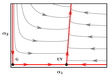
Figure 1: The basic setup in the plane of gauge couplings $(\alpha_{1},\alpha_{2})$, showing the free Gaussian fixed point (G) and an interacting ultraviolet fixed point (UV), with arrows on RG trajectories pointing from the UV to the IR. Note that the Gaussian is a “saddle” and asymptotic freedom is absent.

Here, we apply this methodology exemplarily to an asymptotically non-free $SU(N_{1})\times SU(N_{2})$ supersymmetric gauge theory with massless chiral matter and a superpotential, and determine the entire conformal window of interacting UV fixed points. Our basic setup is illustrated in Fig. 1 which shows the phase diagram of a semi-simple gauge theory with superpotential interactions. Notice that asymptotic freedom is absent because one of the gauge sector $(\alpha_{2})$ is infrared free while the other not $(\alpha_{1})$. The theory may nevertheless develop an asymptotically safe fixed point (UV) which allows as well-defined high energy limit and outgoing RG trajectories towards the IR, and which is the central topic of this study. Consistency with Seiberg duality, and constraints from the $a$-theorem, global charges, and unitarity, are also observed [27]. Findings are confirmed independently using perturbation theory up to three loop order. Implications of our findings for the asymptotic safety conjecture, model building, and conformal field theory are indicated.

Matter	$\bm{\psi_{L}}$	$\bm{\psi_{R}}$	$\bm{\Psi_{L}}$	$\bm{\Psi_{R}}$	$\bm{\chi_{L}}$	$\bm{\chi_{R}}$	$\bm{Q_{L}}$	$\bm{Q_{R}}$
$\ \ \bm{SU(N_{1})}\ \$	$\overline{\Box}$	$\Box$	$\Box$	$\overline{\Box}$	1	1	1	1
$\bm{SU(N_{2})}$	1	1	$\Box$	$\overline{\Box}$	$\overline{\Box}$	$\Box$	$\overline{\Box}$	$\Box$
Flavour	$N_{F}$	$N_{F}$	1	1	$N_{F}$	$N_{F}$	$N_{Q}$	$N_{Q}$

Table 1: Chiral matter with gauge charges and multiplicities.

II Semi-Simple Gauge Theories with Matter

We consider semi-simple Yang-Mills theories with product gauge group $SU(N_{1})\times SU(N_{2})$ coupled to chiral superfields $(\psi,\chi,\Psi,Q)$ with flavour multiplicities $(N_{F},N_{F},1,N_{Q})$ and gauge charges as in Tab. 1. We require that the model has a global $N=1$ supersymmetry. It is then characterised by two gauge couplings $g_{1}$ and $g_{2}$ and a Yukawa coupling $y$ via the superpotential

$$W=y\,{\rm Tr}\big{[}\psi_{L}\,\Psi_{L}\,\chi_{L}+\psi_{R}\,\Psi_{R}\,\chi_{R}\big{]}\,,$$ (1)

where the trace sums over flavour and gauge indices. The superfields $Q$ are not furnished with Yukawa interactions. The theory has a global $SU(N_{F})_{L}\times SU(N_{F})_{R}\times SU(N_{Q})_{L}\times SU(N_{Q})_{R}$ flavour and a $U(1)_{R}$ symmetry and is characterised by the field multiplicities

$$(N_{1}\,,\,N_{2}\,,\,N_{F}\,,\,N_{Q})\,.$$ (2)

Asymptotic freedom and interacting infrared fixed points arise for suitable matter field multiplicities. For this study, the regime of interest is where the $SU(N_{1})$ gauge sector is asymptotically free while the $SU(N_{2})$ gauge sector is infrared free. Accordingly, the free theory corresponds to a “saddle” and asymptotic freedom cannot be achieved (Fig. 1), very much like in the non-abelian gauge sectors of the Minimal Supersymmetric Standard Model (MSSM). In this light, the gauge coupling $\alpha_{2}$ can be viewed as “dangerously irrelevant”, in that it may to become relevant due to the gauge-Yukawa fixed point in the other gauge sector.

In the large $N$ Veneziano limit, the theory has previously been studied in perturbation theory, where it was found that interacting UV fixed points can arise at weak coupling with perturbatively small anomalous dimensions [11]. The main point of this study is to investigate the conditions under which theories with (6) may develop strongly interacting ultraviolet fixed points where anomalous dimensions become large, of order unity. Ordinarily, this would require strong coupling methods such as lattice simulations to establish the claim. In supersymmetry, however, powerful continuum methods beyond perturbation theory are available to which we turn next.

III Renormalisation Group

To achieve our claim, we must find the renormalisation group equations for all couplings and identify their fixed points, and non-perturbative expressions for the chiral superfield anomalous dimensions. Here, we exploit key features of $N=1$ supersymmetic gauge theories which make this task feasible.

For supersymmetric gauge theories, closed all-order expressions for perturbative $\beta$-functions have been achieved by Novikov, Shifman, Vainstein, and Zakharov (NSVZ) [24, 25] (see also [28, 29]). We introduce the gauge and Yukawa couplings as

$$\alpha_{1,2}=\left(\frac{g_{1,2}}{4\pi}\right)^{2}\,,\quad\quad\alpha_{y}=\left(\frac{y}{4\pi}\right)^{2}\,,$$ (3)

and denote the chiral superfield anomalous dimensions as $\gamma_{a}$ $(a=\psi,\Psi,\chi,Q)$, with $\beta$-functions $\beta_{i}\equiv d\alpha_{i}/d\ln\mu$ $(i=1,2,y)$ defined as usual. The NSVZ beta functions for the gauge couplings of our models are then given by

$$\beta_{1} = \frac{2\alpha_{1}^{2}}{F(\alpha_{1})}[N_{F}\left(1-2\gamma_{\psi}\right)+N_{2}\left(1-2\gamma_{\Psi}\right)-3N_{1}]$$ (4)

$$\beta_{2} = \frac{2\alpha_{2}^{2}}{F(\alpha_{2})}[N_{F}\left(1-2\gamma_{\chi}\right)+N_{1}\left(1-2\gamma_{\Psi}\right)+N_{Q}\left(1-2\gamma_{Q}\right)-3N_{2}]\,.$$ (5)

The scheme-dependent function $F(\alpha)$ is normalised to unity for vanishing coupling [30] and reads $F(\alpha)=1-2C^{G}_{2}\alpha$ in the NSVZ scheme [24, 25] with $C^{G}_{2}$ the quadratic Casimir in the adjoint. Close to the Gaussian fixed point, the anomalous dimensions vanish and we can then read off the condition for a saddle in terms of the field multiplicities (2),

$$\begin{array}[]{lcl}3{N_{1}}&>&{N_{2}+N_{F}}\\[4.30554pt] 3N_{2}&\leq&{N_{1}+N_{F}+N_{Q}}\,.\end{array}$$ (6)

This also covers the case where the one-loop coefficient of $\beta_{2}$ vanishes identically. For the Yukawa coupling, we exploit that supersymmetry dictates strict non-renormalisation theorems which ensure that superpotential couplings are only renormalised through field anomalous dimensions. Hence, the RG running is given by

$$\beta_{y} = 2\alpha_{y}\big{[}\gamma_{\psi}+\gamma_{\Psi}+\gamma_{\chi}\big{]}\,,$$ (7)

valid to all orders in perturbation theory. Renormalisation group fixed points $(\beta_{i}=0)$ correspond to superconformal field theories.

All perturbative fixed points $(\alpha^{*}_{i}\ll 1)$ for this theory have previously been found in [11]. In general, these are either Banks-Zaks fixed points where some of the gauge couplings are non-zero but $\alpha^{*}_{y}=0$, or gauge-Yukawa (GY) fixed points with one $({\rm GY}_{1})$, the other $({\rm GY}_{2})$, or both gauge couplings non-zero $({\rm GY}_{12})$ and $\alpha^{*}_{y}>0$ [7, 6]. It has also been shown that if ${\rm GY}_{1}$ is UV, its outgoing trajectory is connected with the IR fixed point $({\rm GY}_{12})$, and similarly for ${\rm GY}_{2}$ [11].

In this work, we focus on the regime (6) and search for non-perturbative fixed points with the property

$${\rm GY}_{1}:\quad\quad\alpha_{1}^{*}>0\,,\quad\alpha_{y}^{*}>0\,,\quad\alpha_{2}^{*}=0\,.$$ (8)

Our ansatz states that the $SU(N_{2})$ gauge sector is infrared free, meaning $\beta_{2}>0$ in the vicinity of the Gaussian. If $\beta_{2}<0$ in the vicinity of the interacting fixed point, the $SU(N_{2})$ gauge sector suddenly becomes asymptotically free, and the fixed point is ultraviolet. In its vicinity, $\alpha_{2}$ is the only relevant coupling in the UV, which runs out of the fixed point as

$$\alpha_{2}(\mu)=\frac{\delta\alpha_{2}(\Lambda)}{1+B_{2,\rm eff}\,\delta\alpha_{2}\,\ln(\mu/\Lambda)}\,,$$ (9)

with $\delta\alpha_{2}(\Lambda)$ a small deviation at the high scale $\Lambda$, $B_{2,\rm eff}=B_{2}+N_{F}\,\gamma_{\chi}+4N_{1}\,\gamma_{\Psi}>0$ the interaction-induced one loop coefficient, and $B_{2}<0$ given by (minus) the one-loop coefficient of (5) at the Gaussian. The couplings $\alpha_{1}$ and $\alpha_{y}$ are irrelevant interactions in the UV and their running is fully determined by the one of $\alpha_{2}$ [11]. This scenario is schematically depicted in Fig. 1.

The necessary and sufficient conditions for the partially interacting fixed point to turn the dangerously irrelevant coupling $\alpha_{2}$ into a relevant one are given by

$$0 = 3N_{1}-N_{F}\left(1-2\gamma_{\psi}\right)-N_{2}\left(1-2\gamma_{\Psi}\right)$$

$$0 < 3N_{2}-N_{F}\,\left(1-2\gamma_{\chi}\right)-N_{1}\left(1-2\gamma_{\Psi}\right)-N_{Q}\left(1-2\gamma_{Q}\right)\,,$$ (10)

$$0 = \gamma_{\psi}+\gamma_{\Psi}+\gamma_{\chi}\,,$$

where the two equations determine the fixed point while the inequality ensures the sign flip from $\beta_{2}\geq 0$ close to the Gaussian to $\beta_{2}<0$ close to the fixed point (8).

IV a-Maximisation

The beta functions (4), (5) and (7), and the conditions (10), still depend on the superfield anomalous dimensions. These can be determined either perturbatively, as we will do in Sec. VIII below, or exactly, as we do here. To that end, we exploit that fixed points of the renormalisation group correspond to superconformal field theories. Hence superfields must transform in representations of the superconformal algebra. Focussing on the bosonic part, we observe an extra global $U(1)_{R}$ symmetry in addition to the ordinary conformal algebra. The global and anomaly-free $U(1)_{R}$ symmetry prescribes global charges $R_{i}$ for all chiral superfields at any superconformal fixed point and thereby determines anomalous dimensions $\gamma_{i}$ of chiral superfields via

$$\gamma_{i}=\frac{3}{2}R_{i}-1\,.$$ (11)

The task then reduces to the determination of $R$-charges at superconformal fixed points for which we use the method of $a$-maximisation [26]. Specifically, at the fixed point GY₁ with (8) and characterised by (10), we find

$$\begin{array}[]{rl}R_{\psi}&\displaystyle=\frac{2}{3}\left(1+\gamma_{\psi}\right)=\frac{N_{F}[N_{F}-(N_{1}+N_{2})]^{2}-N_{1}^{2}\,N_{2}\,\Delta}{[N_{2}-N_{F}][N_{1}(N_{2}+N_{F})+(N_{2}-N_{F})^{2}]}\,,\par\\[10.76385pt] R_{\Psi}&\displaystyle=\frac{2}{3}\left(1+\gamma_{\Psi}\right)=\frac{N_{2}[N_{2}-(N_{1}+N_{F})]^{2}-N^{2}_{1}\,N_{F}\,\Delta}{[N_{F}-N_{2}][N_{1}(N_{2}+N_{F})+(N_{2}-N_{F})^{2}]}\,,\\[10.76385pt] R_{\chi}&=\displaystyle\frac{2}{3}\left(1+\gamma_{\chi}\right)=\frac{8}{9}\frac{(N_{2}-N_{F})^{2}}{(N_{2}-N_{F})^{2}-(1-\Delta)N_{1}^{2}}\,,\\[10.76385pt] R_{Q}&\displaystyle=\frac{2}{3}\left(1+\gamma_{Q}\right)=\frac{2}{3}\,,\end{array}$$ (12)

and $\Delta>0$ the positive root of

$$\Delta^{2} = 1+\left(\frac{N_{2}-N_{F}}{3N_{1}^{2}}\right)^{2}\left[(4N_{1}+N_{2}+N_{F})^{2}-34N_{1}^{2}-4N_{2}N_{F}\right]\,.$$ (13)

The $\psi_{Q}$ fermions do not interact at the fixed point (8), hence $\gamma_{Q}=0$ and none of the $R$-charges depends on $N_{Q}$. The results for the $R$-charges uniquely determine the remaining anomalous dimensions non-perturbatively, and provide closure for the beta functions (4), (5) and (7). At weak coupling, anomalous dimensions are small and $R$-charges are close to their classical values $(R_{i}\approx\mbox{\small{$\frac{2}{3}$}})$. Moreover, unitarity mandates that scaling dimensions $D$ of spinless operators must satisfy $D\geq 1$ [27], additionally implying $\gamma_{i}\geq-\mbox{\small{$\frac{1}{2}$}}$ ($R_{i}\geq\mbox{\small{$\frac{1}{3}$}}$) for gauge-invariant scalar operators such as $\bar{\psi}\psi$.

The conditions for unitary quantum field theories with interacting UV fixed points (10) only depend on ratios of field multiplicities. Therefore, we can reduce the four-dimensional parameter space of field multiplicities (2) to a three-dimensional one. Following [11], we do so by scaling-out one of the field multiplicities, say $N_{1}$, and by introducing three suitable ratios of field multiplicities instead,

$$\begin{array}[]{rcl}R&=&\displaystyle\frac{N_{2}}{N_{1}}\,,\quad P=\frac{N_{1}}{N_{2}}\frac{N_{Q}+N_{1}+N_{F}-3N_{2}}{N_{F}+N_{2}-3N_{1}}\,,\quad\epsilon=\displaystyle\frac{N_{F}+N_{2}}{N_{1}}-3\,.\end{array}$$ (14)

The colour ratio $R$ (not to be confused with the $R$-charges $R_{i}$) is sensitive to the relative size of gauge groups. The parameter $P<0$ is proportional to the ratio of one-loop gauge coefficients. The parameter $\epsilon$, which in the region of interest is negative $\epsilon<0$, can be made arbitrarily small in a Veneziano limit where it controls perturbative fixed points provided $|\epsilon|\ll 1$. Since field multiplicities are semi-positive numbers, we further observe

$$0<R<3\,,\quad P<\frac{4(1-R)+\epsilon}{R\,\epsilon}\,,\quad R-3<\epsilon<0\,.$$ (15)

The parameters (14) take discrete values for integer field multiplicities except in a Veneziano large-$N$ limit where they become continuous.

V Fixed Points and Conformal Windows

We are now in a position to investigate the range of field multiplicities for which the theory displays an interacting ultraviolet fixed point. Exploiting all constraints we find that the parameter $P$ is bounded from above and from below

$$P_{\rm min}(R,\epsilon)<P\leq P_{\rm max}(R,\epsilon)\,.$$ (16)

The upper boundary $P_{\rm max}$ relates to (6) and $P\leq 0$, and to the physicality of field multiplicities (15), whichever is stronger. The lower boundary $P_{\rm min}$ relates to the sign-flip for induced asymptotic freedom of $SU(N_{2})$. Explicitly,

$$P_{\rm max}(R,\epsilon) = \left\{\begin{array}[]{cl}\displaystyle\frac{4(1-R)+\epsilon}{R\,\epsilon}&\ \ {\rm for}\ \ R<1+\frac{\epsilon}{4}\\[8.61108pt] 0&\ \ {\rm otherwise}\end{array}\right.$$ (19)

$$P_{\rm min}(R,\epsilon) = \frac{3R_{\Psi}-2}{R\,\epsilon}+\frac{(3\,R_{\chi}-2)\,(3-R+\epsilon)}{R\,\epsilon}\,.$$ (20)

In the above, the $R$-charges $R_{\Psi}$ and $R_{\chi}$ are understood as functions of $(R,\epsilon)$ via (12) and (14). The parameters $R$ and $\epsilon$ are constrained globally by the physicality of couplings ($\alpha\geq 0$) and unitarity,

$$\begin{array}[]{rcl}\mbox{\small{$\frac{1}{4}$}}<&R&<2\quad{\rm and}\quad-\mbox{\small{$\frac{3}{2}$}}\leq\epsilon<0\,.\end{array}$$ (21)

Fig. 2 shows a contour plot of the superconformal window (16) and (21) in the $(\epsilon,R)$ plane. The left panel shows the lower boundary $P_{\rm min}$ while the right panel shows the accessible range of $P$ values between $P_{\rm min}$ and $P_{\rm max}$. The lower boundary in both graphs is given by $R_{\rm min}=1+\mbox{\small{$\frac{\epsilon}{2}$}}$, corresponding to $N_{1}+N_{2}=N_{F}$. Above the full white line $R=1+\mbox{\small{$\frac{\epsilon}{4}$}}$ we have $P_{\rm max}=0$. Roughly speaking, the width in $P$ is largest around the full white line. At the upper border we have $R_{\rm max}=2+\mbox{\small{$\frac{2}{3}$}}\epsilon$ which translates into $N_{2}=N_{F}$. We notice that the width $P_{\rm max}-P_{\rm min}$ vanishes at $R_{\rm min}$, while it remains small but non-zero at $R_{\rm max}$, except at the endpoints. Weakly coupled fixed points correspond to parameters $(P,R,\epsilon)$ close to the boundary where $|\epsilon|\ll 1$.

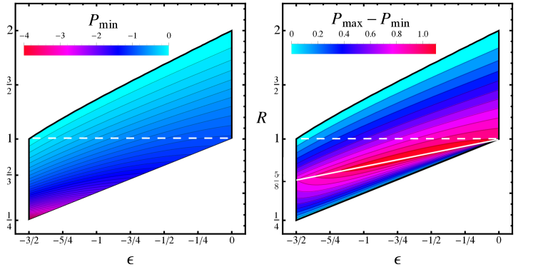
Figure 2: Contour plot of the superconformal window for asymptotic safety (16) in the $(R,\epsilon)$ plane showing the boundary $P_{\rm min}$ (left) and the height $P_{\rm max}-P_{\rm min}$ (right); dashed and full white lines are explained in the main text.

The conformal window is further illustrated in Fig. 3 showing its projection onto the $(P,R)$ plane. Within the yellow-shaded area, weakly coupled fixed points arise towards the right of the dashed line, while strongly-coupled fixed points can arise anywhere. Outside the yellow-shaded area, asymptotic safety is not available and the corresponding quantum field theories must viewed as effective rather than fundamental.

It is interesting to discuss the $N_{F}$ dependence of fixed points within the conformal window while keeping $(N_{1},N_{2},P)$ fixed. In Fig. 2, this effectively corresponds to varying $\epsilon$ along horizontal cuts. We notice that the conformal window splits into two distinct types of models, separated by dashed lines in Figs. 2 and 3, to which we refer as “mostly weakly” and “mostly strongly” coupled. Specifically, the first subset of models are those above the dashed line in Fig. 2 and on the right of the dashed line in Fig. 3. Their conformal window is characterised by

$$\begin{array}[]{rcl}1\leq&R&<2\,.\end{array}$$ (22)

Then, for any admissible value of $R$ within (22), there is a range of viable parameters $P$ within $(-1,0]$ such that the UV conformal window in $\epsilon$ covers the range

$$\epsilon_{\rm max}\leq\epsilon<0\,.$$ (23)

The lower bound $\epsilon_{\rm max}=\mbox{\small{$\frac{3}{2}$}}(R-2)$ may become as low as $-\mbox{\small{$\frac{3}{2}$}}$. The significance of this result is as follows. Perturbative fixed points are controlled by the parameter $|\epsilon|\ll 1$ in a large-$N$ Veneziano limit, meaning that this part of the UV conformal window contains all perturbatively controlled superconformal UV fixed points found previously in [11]. Hence, we observe that all perturbative fixed points extend into a non-perturbative conformal window for $\epsilon$ given precisely by the range (23). The same considerations apply for finite $N$, away from a Veneziano limit, the only difference being that $(R,P,\epsilon)$ take discrete rather than continuous values. Since all theses fixed points are linked to weakly coupled ones, and for want of terminology, we refer to the models within (22) as “mostly weakly” coupled.

Next, we turn to the part of the conformal window below the dashed line in Fig. 2 and to the left of the dashed line in Fig. 3, characterised by

$$\begin{array}[]{rcl}\mbox{\small{$\frac{1}{4}$}}<&R&<1\,.\end{array}$$ (24)

For any admissible value of $R$ within (24), there is a range of viable parameters $P$ within $(-4,0]$ such that the UV conformal window in $\epsilon$ covers the range

$$-\mbox{\small{$\frac{3}{2}$}}\leq\epsilon<\epsilon_{\rm min}<0\,.$$ (25)

Here, the lower bound $\epsilon_{\rm min}=2(R-1)<0$ ensures induced asymptotic freedom for the coupling $\alpha_{2}$. Most importantly, we observe the existence of a finite gap $[\epsilon_{\rm min},0]$ in $\epsilon$ within which no asymptotically safe fixed points can be found. This implies that none of the fixed points within (24) can be achieved with strict perturbative control $(\epsilon\to 0^{-})$, not even in a Veneziano limit. It is in this sense that the fixed points within (24) are non-perturbative and parametrically disconnected from the free theory, quite different from those in (22). For these reasons, we refer to these superconformal fixed points as “mostly strongly” coupled.

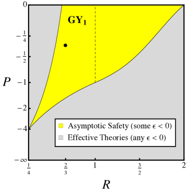
Figure 3: Projection of the superconformal window with interacting ultraviolet fixed points onto the $(R,P)$ parameter plane. Weakly coupled fixed points arise within the yellow-shaded area on the right of the dashed line. Strongly-coupled fixed points arise within the entire yellow-shaded area for some range of $\epsilon$. The full dot is discussed in the main text.

Another important aspect of the conformal window relates to the saddle close to the Gaussian which needs to be overcome by the interacting fixed point. Recall that the asymptotically free (infrared free) direction is characterised by the one-loop gauge coefficient $B_{1}=2\,N_{1}\,\epsilon<0$ ($B_{2}=2\,N_{2}\,P\,\epsilon\geq 0$), with (minus) their ratio given by the imbalance parameter

$$I=-B_{2}/B_{1}\equiv|P|\cdot R$$ (26)

for which we have $I\geq 0$. Quantum effects at the interacting fixed point overcome the positive or vanishing one-loop coefficient $B_{2}$ and turn it, effectively, into a negative one (see Fig. 1). It is then important to understand the largest imbalance that can be achieved without spoiling asymptotic safety. We find that the imbalance is bounded from above,

$$0\leq I=\frac{3N_{2}-N_{1}-N_{F}-N_{Q}}{N_{F}+N_{2}-3N_{1}}<1\,,$$ (27)

where we recall that field multiplicities obey (6). In other words, as soon as one gauge sector is as or more infrared free at the Gaussian fixed point than the other gauge sector is ultraviolet free, asymptotic safety at an interacting fixed point cannot arise.

In Figs. 2 and 3, the small imbalance region $0\leq I\ll 1$ is realised close to the upper boundaries where $P\approx 0$. Here, many ultraviolet fixed points can be found in large parts of the parameter space including perturbative and non-perturbative ones. With growing imbalance $I\to 1$, the set of perturbatively controlled fixed points shrinks to the vicinity of a single point $(P,R)=(-1,1)$. Non-perturbatively, however, many more fixed points realise a near-maximal imbalance, corresponding to the lower boundary in Fig. 2 with parameters given by the line $R=R_{\rm min}(\epsilon)$, $P=-1/R_{\rm min}$, and $\epsilon\in[-\mbox{\small{$\frac{3}{2}$}},0)$. In Fig. 3, the near-maximal imbalance is realised along the lower boundary to the left of the dashed line. We conclude that all models which may afford the near-maximal imbalance are contained in the “mostly strongly coupled” part of the conformal window (24).

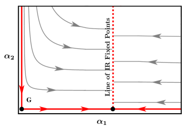
Figure 4: Schematic phase diagram of Leigh-Strassler type models in the plane of gauge couplings in the limit where the UV fixed point degenerates into a line of IR fixed points (see Fig. 1).

We emphasize that the boundary at $P_{\rm min}$ in (20) is not part of the conformal window. The reason for this is that whenever $P\to P_{\rm min}$ the inequality in (10) becomes an equality, meaning that $\beta_{2}\to 0$ non-perturbatively at the fixed point (8). At this point the UV fixed point ${\rm GY}_{1}$ merges with yet another fixed point (a non-perturbative IR fixed point ${\rm GY}_{12}$ [11]) in the limit $P\to P_{\rm min}$. In consequence, the fixed point (8) degenerates into a line of fixed points for any $\alpha_{2}$, illustrated in Fig. 4. As such, this limit offers a manifold of Leigh-Strassler type models [31], each of which is characterised by a line of interacting superconformal field theories, disconnected from the free theory, and generated by an exactly marginal operator. Further, each of these lines of fixed points corresponds to an infrared sink because the previously relevant perturbation, given by $\alpha_{2}$, has become strictly marginal. This includes all settings with maximal imbalance $I=1$. Concrete examples for strongly-coupled Leigh-Strassler models are delegated to Sec. X below.

Fig. 5 shows the superfield anomalous dimensions within the entire conformal window. Since the spectator fermions $\psi_{Q}$ are free at the fixed point (8), the chiral superfield anomalous dimensions are only functions of $(R,\epsilon)$ and independent of $P$. Overall, we find that anomalous dimensions grow with growing $|\epsilon|$. For models within (22) or (24), the chiral anomalous dimensions cover the range

$$0>\gamma_{\psi},\gamma_{\Psi}\geq-\mbox{\small{$\frac{1}{2}$}}\quad{\rm and}\quad 0<\gamma_{\chi}\leq 1$$ (28)

with extremals reached at the $\epsilon=-\mbox{\small{$\frac{3}{2}$}}$ and $\epsilon=0$ boundaries of the conformal window. For models within (24) anomalous dimensions tend to take larger values than for those in (22). A comparison with perturbation theory is given in Sec. VIII. Incidentally, the monotonicity of $\gamma_{i}$ with growing $\epsilon$ establishes that anomalous dimensions do not vanish unless the fixed point is free.

VI Central Charges and the $a$-Theorem

Superconformal fixed points can also be characterised by central charges $a$, $b$ and $c$, the anomaly coefficients [32, 33]. Their values have to satisfy certain conditions, and can be used to constrain viable fixed points. The global charges $a$ and $c$ can be expressed in terms of the $R$-charges of chiral superfields,

$$a =\frac{3}{32}\left(3{\rm Tr}R^{3}-{\rm Tr}R\right)\,$$ (29)

$$c =\frac{1}{32}\left(9{\rm Tr}R^{3}-5{\rm Tr}R\right)\,.$$ (30)

Given that the positivity conditions $a,b,c>0$ are satisfied non-marginally for free theories, they are guaranteed to be satisfied for perturbative theories. Similarly, the conformal collider bound [34]

$$\frac{1}{2}<\frac{a}{c}<\frac{3}{2}$$ (31)

cannot be violated for weakly interacting theories. Here, we find that the positivity conditions and the conformal collider bound are satisfied non-perturbatively, in the entire conformal window, as they must.

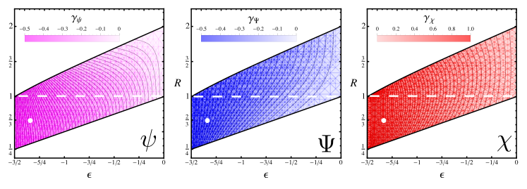
Figure 5: Contour plot showing the non-perturbative anomalous dimensions of chiral superfields at the superconformal fixed points of Fig. 2. The full dot and dashed line are explained in the main text.

We now turn to the $a$-theorem. It states that the central charge $a$ must be a decreasing function along RG trajectories in any 4d quantum field theory [35, 36]. We find that $a_{\rm UV}-a_{\rm Gauss}<0\,,$ which confirms that none of the UV fixed points is connected by an RG trajectory with the free Gaussian fixed point, in accord with Fig. 1. Further, we noted earlier that any interacting UV fixed point in the conformal window comes bundled with a fully interacting non-perturbative IR fixed point $({\rm GY}_{12})$ [11]. We find $a_{\rm UV}-a_{\rm IR}>0\,,$ meaning that both conformal fixed points are connected by RG trajectories flowing from the former to the latter as in Fig. 1. We conclude that our results are consistent with the $a$-theorem, as they must.

VII Seiberg Duality

Next, we comment on how our results relate to Seiberg’s electric-magnetic duality [37]. At the partially interacting fixed point (8) where the $SU(N_{2})$ gauge sector is free, the flavour symmetry of the theory is enhanced. This manifests itself as an exchange symmetry under $N_{2}\leftrightarrow N_{F}$, whereby the quarks $\psi$ and $\Psi$ interchange their roles while the fields $\chi$ remain unchanged,

$$N_{2}\leftrightarrow N_{F}\,,\quad\quad R_{\psi}\leftrightarrow R_{\Psi}\,,\quad\quad R_{\chi}\leftrightarrow R_{\chi}\,,$$ (32)

see (12). Hence, we observe an interacting “magnetic” $SU(N_{1})$ gauge theory which has $N_{F}+N_{2}$ flavours of “magnetic quarks” $\psi$ and $\Psi$, alongside $(N_{F}+N_{2})^{2}$ singlet mesons $(\psi_{L}\psi_{R})$, $\chi_{L}$, $\chi_{R}$, and $(\Psi_{L}\Psi_{R})$ [38]. In this light, the gauge-Yukawa fixed point (8) corresponds to a free non-Abelian magnetic phase whose superconformal window is known to cover the range $\mbox{\small{$\frac{3}{2}$}}N_{1}<N_{F}+N_{2}<3N_{1}$ [37] which corresponds to the parameter range $-\mbox{\small{$\frac{3}{2}$}}<\epsilon<0$ observed in (21). Notice however that the conformal window in Fig. 2 has additional constraints on $(R,P)$ which ensure that the $SU(N_{2})$ gauge sector becomes a relevant perturbation at the fixed point.

Seiberg duality predicts the existence of a dual “electric” theory which must have gauge group $SU(N_{F}+N_{2}-N_{1})$ coupled to $N_{F}+N_{2}$ flavours of electric quarks. The conformal window of the non-Abelian Coulomb phase is given by $\mbox{\small{$\frac{3}{2}$}}(N_{F}+N_{2}-N_{1})<N_{F}+N_{2}<3(N_{F}+N_{2}-N_{1})\,.$ This corresponds to the exact same parameter band in $\epsilon$ as the one in (21). In the special case where $N_{F}=N_{2}$, given by the upper boundary in Fig. 2, the $R$-charges simplify and become

$$R_{\psi}=R_{\Psi}=1-\frac{N_{1}}{2N_{F}}\,,\quad R_{\chi}=\frac{N_{1}}{N_{F}}\,.$$ (33)

One recognises the $R$-charges for the quarks and singlet mesons of supersymmetric magnetic QCD [37], whose Seiberg dual is characterised by electric quarks ${\widetilde{\psi}}$ and $\widetilde{\Psi}$ with

$$R_{\widetilde{\psi}}=R_{\widetilde{\Psi}}=\frac{N_{1}}{2N_{F}}\,.$$ (34)

We refer to [38] for further aspects of Seiberg duality in theories with product gauge groups.

VIII Perturbation Theory

In this section, we contrast the non-perturbative determination of anomalous dimensions with perturbation theory, using general expressions for perturbative beta functions in the DRED regularisation scheme up to three loop [39, 40]. The main addition are perturbative expressions for anomalous dimensions which at superconformal fixed points can be used to cross-check the non-perturbative results from $a$-maximisation.

For the sake of this comparison, it is convenient to perform a Veneziano limit and rescale gauge couplings as $\alpha_{i}\to N_{i}\,\alpha_{i}$ and Yukawas as $\alpha_{y}\to N_{1}\,\alpha_{y}$. We also use the parametrisation (14). The parameter $0<|\epsilon|\ll 1$ then serves as a small expansion parameter to ensure rigorous control of fixed points in perturbation theory. To find fixed points, scaling exponents, and anomalous dimensions to first (second) order in $\epsilon$, we must retain terms up to two (three) loop in the gauge coupling, and up to one (two) loop in the Yukawa beta functions [7, 22]. We refer to these approximations as NLO and NNLO, respectively. Using the general results of [39, 40] we find the gauge beta functions up to three loop for our models as

$$\beta_{1}^{(1)} = \displaystyle 2\alpha_{1}^{2}\,\epsilon\,,$$

$$\beta_{1}^{(2)} = \displaystyle 2\alpha_{1}^{2}\big{[}6\alpha_{1}+2R\alpha_{2}-4R(3+\epsilon-R)\alpha_{y}\big{]}\,,$$ (35)

$$\beta_{1}^{(3)} = 4\alpha_{1}^{2}\left[2\epsilon\alpha_{1}^{2}-R\left(2\alpha_{1}\,\gamma_{\Psi}^{(1)}+\gamma_{\Psi}^{(2)}\right)-(3+\epsilon-R)\left(2\alpha_{1}\,\gamma_{\psi}^{(1)}+\gamma_{\psi}^{(2)}\right)\right]\,,$$

and

$$\beta_{2}^{(1)} = \displaystyle 2\alpha_{2}^{2}\,P\epsilon\,,$$

$$\beta_{2}^{(2)} = \displaystyle 2\alpha_{2}^{2}\left[6\alpha_{2}+\frac{2}{R}\alpha_{1}-\frac{4}{R}(3-R+\epsilon)\alpha_{y}\right]\,,$$ (36)

$$\beta_{2}^{(3)} = 4\alpha_{2}^{2}\left[2P\epsilon\alpha_{2}^{2}-\frac{1}{R}\left(2\alpha_{2}\gamma_{\Psi}^{(1)}+\gamma_{\Psi}^{(2)}\right)\right.$$

$$\quad\quad\left.-\frac{3-R+\epsilon}{R}\left(2\alpha_{2}\,\gamma_{\chi}^{(1)}+\gamma_{\chi}^{(2)}\right)-\left(4+P\epsilon-\frac{4+\epsilon}{R}\right)\left(2\alpha_{2}\,\gamma_{Q}^{(1)}+\gamma_{Q}^{(2)}\right)\right]\,.$$

The perturbative Yukawa beta function is given by (7) for any loop order. The anomalous dimensions of the superfields are required up to two loop accuracy. They read

$$\begin{array}[]{rcl}\gamma_{\psi}^{(1)}&=&\displaystyle R\,\alpha_{y}-\alpha_{1}\,,\\[4.30554pt] \gamma_{\Psi}^{(1)}&=&\displaystyle(3-R+\epsilon)\alpha_{y}-\alpha_{1}-\alpha_{2}\,,\\[4.30554pt] \gamma_{\chi}^{(1)}&=&\displaystyle\alpha_{y}-\alpha_{2}\,,\\[4.30554pt] \gamma_{Q}^{(1)}&=&\displaystyle-\alpha_{2}\,,\end{array}$$ (37)

and

$$\begin{array}[]{rcl}\gamma_{\psi}^{(2)}&=&\displaystyle-R\,\alpha_{y}\left(\gamma_{\Psi}^{(1)}+\gamma_{\chi}^{(1)}\right)-\alpha_{1}\gamma_{\psi}^{(1)}+4\,\epsilon\,\alpha_{1}^{2}\,,\\[4.30554pt] \gamma_{\Psi}^{(2)}&=&\displaystyle-(3-R+\epsilon)\,\alpha_{y}\left(\gamma_{\psi}^{(1)}+\gamma_{\chi}^{(1)}\right)-(\alpha_{1}+\alpha_{2})\gamma_{\Psi}^{(1)}+4\,\epsilon\,\alpha_{1}^{2}+4\,P\,\epsilon\,\alpha_{2}^{2}\,,\\[4.30554pt] \gamma_{\chi}^{(2)}&=&\displaystyle-\alpha_{y}\left(\gamma_{\psi}^{(1)}+\gamma_{\Psi}^{(1)}\right)-\alpha_{2}\gamma_{\chi}^{(1)}+4\,P\,\epsilon\,\alpha_{2}^{2}\,,\\[4.30554pt] \gamma_{Q}^{(2)}&=&\displaystyle-\alpha_{2}\,\gamma_{Q}^{(1)}+4\,P\,\epsilon\,\alpha_{2}^{2}\,,\end{array}$$ (38)

respectively. Then, interacting fixed points with (8) are determined via a Taylor expansion of couplings in $\epsilon$ around the zeros of (35) and (7), also using (37) and (38). Notice that (36) is only used to determine whether the sign change from $\beta_{2}>0$ at the Gaussian to $\beta_{2}<0$ at (8) has taken place. Inserting the perturbative results for the fixed point into (37) and (38) provides explicit expressions for the anomalous dimensions of the form

$$\gamma_{i}(\epsilon)=A^{(1)}_{i}\,\epsilon+A^{(2)}_{i}\,\epsilon^{2}+{\cal O}(\epsilon^{3})\,.$$ (39)

The six coefficients $A^{(n)}_{i}$ for $i=\psi,\Psi,\chi$ which for $n=1,2$ arise from the perturbative fixed point solutions at NLO and NNLO accuracy [10, 22] still depend on the parameter $R$ (but not on $P$). Their explicit expressions are not given because they do not offer further insights for the present purposes.

The expressions (39) must be compared with the exact $R$-charges from $a$-maximisation (12). Writing the exact anomalous dimensions in terms of the $R$-charges, and expanding the expressions to second order in $\epsilon$ with the help of (14), we find the identical result for the coefficients $A^{(n)}_{i}$ in (39). This establishes consistency of findings between $a$-maximisation and perturbation theory, as it must.

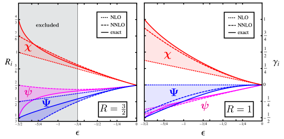
Figure 6: Exact anomalous dimensions and $U(1)_{R}$ charges in comparison with 2-loop (NLO) and 3-loop (NNLO) results from perturbation theory. Shown are projections along $R=\mbox{\small{$\frac{3}{2}$}}$ (left panel) and $R=1$ (right panel). Fixed points in the gray-shaded area do not show the required sign-flip in (10) for any $P$, and are therefore outside of the UV conformal window.

IX Anomalous Dimensions

In Fig. 5 we have shown the exact anomalous dimensions across the entire UV conformal window. Here, we have a closer look into anomalous dimensions and compare with the NLO and NNLO predictions from perturbation theory. More specifically, in Figs. 6 and 7, we compare results at fixed colour ratio $R=\mbox{\small{$\frac{3}{2}$}},1,\mbox{\small{$\frac{2}{3}$}}$ and $\frac{1}{3}$, and for any $\epsilon$ within $[-\mbox{\small{$\frac{3}{2}$}},0]$, which corresponds to horizontal cuts across Figs. 2 and 5.

We begin with Fig. 6 where our results for $R=\mbox{\small{$\frac{3}{2}$}}$ (left panel) and $R=1$ (right panel) are shown. For small $|\epsilon|\ll 1$, perturbation theory matches the exact results as it must. With growing $|\epsilon|$, all anomalous dimensions grow in magnitude. For $R=\mbox{\small{$\frac{3}{2}$}}$, the gray-shaded area indicates that fixed points are no longer in the UV conformal window, leading to a lower bound for $\epsilon$, see (23). Also, the NLO results for $\gamma_{\psi}$ and $\gamma_{\Psi}$ coincide accidentally. At NNLO, perturbative results for all three anomalous dimensions are quite close to the exact results in the admissible range for $\epsilon$. For $R=1$, the extension of the conformal window is maximal. Here, anomalous dimensions correspond to the fixed points along the dashed lines in Figs. 2, 3 and 5, which marks the boundary between the “mostly weakly” and “mostly strongly” coupled quantum field theories, see (22) vs (24). Maximal values $\gamma_{\psi,\Psi}\to-\mbox{\small{$\frac{1}{2}$}}$ and $\gamma_{\chi}\to 1$ are reached for $\epsilon\to-\mbox{\small{$\frac{3}{2}$}}$. For $\gamma_{\psi}$, we observe that the NLO and NNLO results are close to the exact one over the entire range for $\epsilon$. For $\gamma_{\Psi}$, the NLO correction vanishes accidentally. Similarily, for $\gamma_{\chi}$, the NLO result strongly underestimates the exact value with growing $|\epsilon|$. However, at NNLO, perturbative results for all three anomalous dimensions are close to the exact findings in the entire range of $\epsilon$. We conclude that differences between NNLO and exact results are moderate over the entire interval. Note that this does not hold true in general, but when it does, one may use this near-coincidence to extract estimates for fixed points at strong coupling which elsewise are not easily accessible.

The same analysis is repeated in Fig. 7 for the parameter choices $R=\mbox{\small{$\frac{2}{3}$}}$ (left panel) and $R=\mbox{\small{$\frac{1}{3}$}}$ (right panel). These horizontal cuts through Fig. 2 project onto the more strongly coupled fixed points in (24). For either of these the small $\epsilon$ regions are excluded (grey-shaded areas) because the corresponding fixed points are not ultraviolet. In the increasingly narrow regions of interest (25) which are $\epsilon\in[-\mbox{\small{$\frac{3}{2}$}},-\mbox{\small{$\frac{2}{3}$}}]$ and $\epsilon\in[-\mbox{\small{$\frac{3}{2}$}},-\mbox{\small{$\frac{4}{3}$}}]$, respectively, we observe that differences between NLO, NNLO, and exact results become rather large for $\gamma_{\chi}$, $\gamma_{\psi}$ and $\gamma_{\Psi}$. Outside the UV conformal window, we also notice that $\gamma_{\Psi}$ is no longer monotonous with $\epsilon$, but instead changes sign for non-vanishing $\epsilon$, and taking values outside the range (28). Perhaps unsurprisingly, this confirms that the leading orders of perturbation theory cease to offer a good approximation for anomalous dimensions at strong coupling, once $|\epsilon|$ is large.

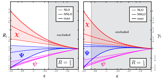
Figure 7: Same as Fig. 6, except that the projections are along $R=\mbox{\small{$\frac{2}{3}$}}$ (left panel) and $R=\mbox{\small{$\frac{1}{3}$}}$ (right panel). Decreasing $R$ considerably narrows the UV conformal window. The excluded (gray-shaded) areas refer to regions where some matter field field multiplicities would be unphysical (negative).

X Benchmarks for Models of Particle Physics

At weak coupling, ultraviolet fixed points are often characterised by a large number of field multiplicities [11]. At strong coupling, fixed points can arise with a much lower number matter fields. Therefore, we benchmark models with minimal numbers of gauge and matter fields and explore whether variants could serve as templates for asymptotically safe Standard Model extensions.

Our benchmarks of superconformal fixed points with low numbers of fields are summarised in Tab. 2. They represent strongly coupled models in that they have large $|\epsilon|$ and anomalous dimensions. The benchmarks also cover the full range of imbalance parameters $I$. Note that because the $\psi_{Q}$ fermions are free at the superconformal fixed point, anomalous dimensions of chiral superfields agree between different models as long as they only differ in the $N_{Q}$ multiplicity, see models 2–4, model 5 and 6, or model 7 and 8.

We begin with model 1 which is the sole example with $SU(2)\times SU(2)$ gauge symmetry, the simple reason being that the only other integer solution $(N_{F},N_{Q})=(3,2)$ to the constraint (6) does not lead to asymptotic safety. Here, anomalous dimensions are still small and well-approximated by the perturbative three loop result (see Fig. 6, right panel). Moreover, in models 1 and 2, the $SU(2)$ gauge sector has a vanishing one-loop coefficient. In both cases a viable interacting UV fixed point is found, located at a boundary of the conformal window (Fig. 2) where $I=0$.

For the gauge group $SU(3)\times SU(2)$, we find a total of five solutions (models 2–6). For all of these $SU(2)$ is infrared free at the Gaussian. Settings where $SU(3)$ is infrared free do not lead to asymptotic safety. Also, all models are within the strongly-coupled domain where 3-loop perturbation theory does not offer an accurate approximation (Fig. 7, left panel). Model 3 has $N_{F}=3$ and $N_{Q}=1$ and its location in the conformal window is indicated by a full dot in Figs. 2 and 3. The anomalous dimensions are of order unity

$$(\gamma_{\psi},\gamma_{\Psi},\gamma_{\chi})\approx(-0.41,-0.38,0.79)$$ (40)

and shown by a full dot in Fig. 5. Enhancing $N_{Q}$ by one unit gives another viable fixed point (model 4) without changing the anomalous dimensions. For $(N_{F},N_{Q})=(4,0)$ (model 5) and $(N_{F},N_{Q})=(4,1)$ (model 6), the main change is that $|\epsilon|$, and hence the anomalous dimensions come out slightly smaller than in model 2-4. Overall, increasing the number of matter fields charged under $SU(2)$ also increases the imbalance parameter.

Models $3-6$ have some similarities with the Minimal Supersymmetric Standard Model (MSSM). Unlike in the Standard Model, the $SU(2)$ sector of the MSSM becomes infrared free due to extra gauge charges from supersymmetry partners, while the $SU(3)$ sector remains asymptotically free. Hence, the Gaussian corresponds to a saddle with imbalance $I_{\rm MSSM}=\mbox{\small{$\frac{1}{3}$}}$, just as in model 5. The imbalance could even be made larger such as in model 4 or model 6, and still yield an asymptotically safe fixed point. Hence, we see that supersymmetric gauge theories with the SM gauge groups (neglecting hypercharge) and imbalances similar to the MSSM may very well become asymptotically safe [41].

Model	Gauge Group	$\bm{N_{F}}$	$\bm{N_{Q}}$	$\bm{I}$	$\bm{R}$	$\bm{P}$	$\bm{\epsilon}$	$\bm{\gamma_{\psi}}$	$\bm{\gamma_{\Psi}}$	$\bm{\gamma_{\chi}}$
1	$SU(2)\times SU(2)$	3	1	$0$	$1$	$0$	$-\mbox{\small{$\frac{1}{2}$}}$	$-0.126$	$-0.061$	$0.187$
2	$SU(3)\times SU(2)$	3	0	$0$	$\frac{2}{3}$	$0$	$-\mbox{\small{$\frac{4}{3}$}}$	$-0.412$	$-0.382$	$0.794$
3	$SU(3)\times SU(2)$	3	1	$\frac{1}{4}$	$\frac{2}{3}$	$-\mbox{\small{$\frac{3}{8}$}}$	$-\mbox{\small{$\frac{4}{3}$}}$	$-0.412$	$-0.382$	$0.794$
4	$SU(3)\times SU(2)$	3	2	$\frac{1}{2}$	$\frac{2}{3}$	$-\mbox{\small{$\frac{3}{4}$}}$	$-\mbox{\small{$\frac{4}{3}$}}$	$-0.412$	$-0.382$	$0.794$
5	$SU(3)\times SU(2)$	4	0	$\frac{1}{3}$	$\frac{2}{3}$	$-\mbox{\small{$\frac{1}{2}$}}$	$-1$	$-0.288$	$-0.174$	$0.462$
6	$SU(3)\times SU(2)$	4	1	$\frac{2}{3}$	$\frac{2}{3}$	$-1$	$-1$	$-0.288$	$-0.174$	$0.462$
7	$SU(6)\times SU(2)$	7	0	$\frac{7}{9}$	$\frac{1}{3}$	$-\mbox{\small{$\frac{7}{3}$}}$	$-\mbox{\small{$\frac{3}{2}$}}$	$-\mbox{\small{$\frac{1}{2}$}}$	$-\mbox{\small{$\frac{1}{2}$}}$	$1$
$8$	$SU(6)\times SU(2)$	7	1	$\frac{8}{9}$	$\frac{1}{3}$	$-\mbox{\small{$\frac{8}{3}$}}$	$-\mbox{\small{$\frac{3}{2}$}}$	$-\mbox{\small{$\frac{1}{2}$}}$	$-\mbox{\small{$\frac{1}{2}$}}$	$1$
$9$	$SU(8)\times SU(2)$	10	0	$1$	$\frac{1}{4}$	$-4$	$-\mbox{\small{$\frac{3}{2}$}}$	$-\mbox{\small{$\frac{1}{2}$}}$	$-\mbox{\small{$\frac{1}{2}$}}$	$1$

Table 2: Parameter and anomalous dimensions for a selection of benchmark models with superconformal fixed points and a low number of field multiplicities, including Leigh-Strassler type models (8 and 9).

The constraints (6) imply that maximal values for anomalous dimensions (28) cannot arise if gauge group factors are as small as $SU(2)$ or $SU(3)$. For larger gauge groups, however, we can find models realising maximal anomalous dimensions. An example is given by an $SU(6)\times SU(2)$ gauge theory with $N_{F}=7$ (model 7) which has a near-maximal imbalance parameter $(I=\mbox{\small{$\frac{7}{9}$}}$). The model is located at the $\epsilon=-\mbox{\small{$\frac{3}{2}$}}$ boundary of the conformal window and leads to an asymptotically safe fixed point with non-perturbatively large chiral field anomalous dimensions,

$$\gamma_{\psi}=-\frac{1}{2}\,,\quad\gamma_{\Psi}=-\frac{1}{2}\,,\quad\gamma_{\chi}=1\,.$$ (41)

We conclude that the benchmark models are low-field-multiplicity realisations of asymptotic safety with phase diagrams as in Fig. 1. Most of them are non-perturbative with large $|\epsilon|$ and large anomalous dimensions, whose features are not captured reliably by a few leading orders of perturbation theory (Fig. 7). With increasing sizes of gauge group factors $(N_{1},N_{2})$, many more solutions $(N_{F},N_{Q})$ for the constraint (6) arise, and a fair fraction of these lead to an asymptotically safe fixed point within the UV conformal window (Fig. 2).

Finally, we discuss two benchmark models with $\epsilon=-\mbox{\small{$\frac{3}{2}$}}$ and maximal anomalous dimensions. These strongly-coupled models are of the Leigh-Strassler type and narrowly outside the UV conformal window. The first one is model 8 with $SU(6)\times SU(2)$ gauge symmetry and $N_{F}=7$, which differs from model 7 only in that $N_{Q}=1$ instead of $N_{Q}=0$, thus leading to a larger imbalance ($I=\mbox{\small{$\frac{8}{9}$}}$). In consequence, the ultraviolet fixed point of model 7 degenerates into a line of fixed points due to $\beta_{2}|_{*}$ vanishing identically at the gauge-Yukawa fixed point. The exactly marginal coupling $\alpha_{2}$ becomes a free parameter and extends the fixed point into an infrared attractive line. The same phenomenon occurs for model 9, which has an $SU(8)\times SU(2)$ gauge symmetry with $N_{F}=10$ and imbalance $I=1$, situated at the lower-left corner of Fig. 2. Although interesting in their own right, the models 8 and 9 no longer serve the purpose of ultraviolet fixed points. However, we stress that the method of $a$-maximisation has been key in identifying fixed points with exactly marginal directions.

XI Conclusions

We have shown, as a proof of principle, that interacting UV fixed points exist in strongly coupled quantum field theories including away from Veneziano (large-$N$) limits. Fixed point anomalous dimensions of matter fields can grow large, taking values in the entire range dictated by unitarity (28). Thereby, previously-found perturbative fixed points [11] extend naturally into a non-perturbative conformal window (Fig. 6). Interestingly, a novel range of fixed points has become available, with no perturbative counterparts in a Veneziano limit (Fig. 7). We thus conclude that the non-perturbative “phase space” of fixed points is large, and substantially larger then the one accessible at weak coupling. Further, all conformal fixed points (Fig. 2) are in accord with the $a$-theorem, bounds on central charges, Seiberg duality, and unitarity. We also found a manifold of Leigh-Strassler models arising at the sign-flip-controlling boundary of the conformal window, where theories display a line of IR fixed points generated by an exactly marginal gauge interaction (Fig. 4). It is understood that similar UV conformal windows, bounded by Leigh-Strassler manifolds, arise naturally in other semi-simple gauge theories coupled to matter.

From the viewpoint of particle physics and model building, it is quite promising that fixed points persist at low field multiplicities (Tab. 2), including with Standard Model-like gauge groups. Next natural questions to ask are whether fixed points also arise in MSSM extensions [41] or in non-supersymmetric setting at strong coupling. From the viewpoint of conformal field theory, it will be interesting to classify asymptotically safe SUSY theories more systematically, and to extract CFT data or structure coefficients directly from the RG fixed points.

Acknowledgements

The work of DL is supported by the Science and Technology Research Council (STFC) under the Consolidated Grant [ST/T00102X/1] .

References

- [1] D. J. Gross and F. Wilczek, Ultraviolet Behavior of Nonabelian Gauge Theories, Phys.Rev.Lett. 30 (1973) 1343.
- [2] H. D. Politzer, Reliable Perturbative Results for Strong Interactions?, Phys.Rev.Lett. 30 (1973) 1346.
- [3] S. Weinberg, Ultraviolet divergences in quantum theories of gravitation, in: General Relativity: An Einstein centenary survey, Eds. Hawking, S.W., Israel, W; Cambridge University Press (1979) 790.
- [4] D. Bailin and A. Love, Asymptotic Near Freedom, Nucl. Phys. B75 (1974) 159.
- [5] D. F. Litim and F. Sannino, Asymptotic safety guaranteed, JHEP 12 (2014) 178 [1406.2337].
- [6] A. D. Bond and D. F. Litim, Price of Asymptotic Safety, Phys. Rev. Lett. 122 (2019) 211601 [1801.08527].
- [7] A. D. Bond and D. F. Litim, Theorems for Asymptotic Safety of Gauge Theories, Eur. Phys. J. C77 (2017) 429 [1608.00519].
- [8] A. Bond and D. F. Litim, Interacting ultraviolet completions of four-dimensional gauge theories, PoS LATTICE2016 (2017) 208.
- [9] A. D. Bond, D. F. Litim and T. Steudtner, Asymptotic safety with Majorana fermions and new large equivalences, Phys. Rev. D 101 (2020) 045006 [1911.11168].
- [10] A. D. Bond and D. F. Litim, More asymptotic safety guaranteed, Phys. Rev. D 97 (2018) 085008 [1707.04217].
- [11] A. D. Bond and D. F. Litim, Asymptotic safety guaranteed in supersymmetry, Phys. Rev. Lett. 119 (2017) 211601 [1709.06953].
- [12] A. D. Bond, G. Hiller, K. Kowalska and D. F. Litim, Directions for model building from asymptotic safety, JHEP 08 (2017) 004 [1702.01727].
- [13] K. Kowalska, A. Bond, G. Hiller and D. Litim, Towards an asymptotically safe completion of the Standard Model, PoS EPS-HEP2017 (2017) 542.
- [14] G. Hiller, C. Hormigos-Feliu, D. F. Litim and T. Steudtner, Asymptotically safe extensions of the Standard Model with flavour phenomenology, in 54th Rencontres de Moriond on Electroweak Interactions and Unified Theories, pp. 415–418, 2019, 1905.11020.
- [15] G. Hiller, C. Hormigos-Feliu, D. F. Litim and T. Steudtner, Anomalous magnetic moments from asymptotic safety, Phys. Rev. D 102 (2020) 071901 [1910.14062].
- [16] G. Hiller, C. Hormigos-Feliu, D. F. Litim and T. Steudtner, Model Building from Asymptotic Safety with Higgs and Flavor Portals, Phys. Rev. D 102 (2020) 095023 [2008.08606].
- [17] S. Bißmann, G. Hiller, C. Hormigos-Feliu and D. F. Litim, Multi-lepton signatures of vector-like leptons with flavor, Eur. Phys. J. C 81 (2021) 101 [2011.12964].
- [18] R. Bause, G. Hiller, T. Höhne, D. F. Litim and T. Steudtner, B-anomalies from flavorful U(1)′ extensions, safely, Eur. Phys. J. C 82 (2022) 42 [2109.06201].
- [19] D. F. Litim, M. Mojaza and F. Sannino, Vacuum stability of asymptotically safe gauge-Yukawa theories, JHEP 01 (2016) 081 [1501.03061].
- [20] T. Buyukbese and D. F. Litim, Asymptotic safety of gauge theories beyond marginal interactions, PoS LATTICE2016 (2017) 233.
- [21] S. Abel and F. Sannino, Radiative Symmetry Breaking from Interacting UV Fixed Points, Phys. Rev. D 96 (2017) 056028 [1704.00700].
- [22] A. D. Bond, D. F. Litim, G. Medina Vazquez and T. Steudtner, UV conformal window for asymptotic safety, Phys. Rev. D 97 (2018) 036019 [1710.07615].
- [23] A. D. Bond, D. F. Litim and G. M. Vazquez, Conformal windows beyond asymptotic freedom, Phys. Rev. D 104 (2021) 105002 [2107.13020].
- [24] V. Novikov, M. A. Shifman, A. Vainshtein and V. I. Zakharov, Exact Gell-Mann-Low Function of Supersymmetric Yang-Mills Theories from Instanton Calculus, Nucl. Phys. B 229 (1983) 381.
- [25] V. Novikov, M. A. Shifman, A. Vainshtein and V. I. Zakharov, The Beta Function in Supersymmetric Gauge Theories. Instantons Versus Traditional Approach, Sov. J. Nucl. Phys. 43 (1986) 294.
- [26] K. A. Intriligator and B. Wecht, The Exact superconformal R symmetry maximizes a, Nucl. Phys. B667 (2003) 183 [hep-th/0304128].
- [27] G. Mack, All Unitary Ray Representations of the Conformal Group SU(2,2) with Positive Energy, Commun. Math. Phys. 55 (1977) 1.
- [28] K. Stepanyantz, The all-loop perturbative derivation of the NSVZ -function and the NSVZ scheme in the non-Abelian case by summing singular contributions, Eur. Phys. J. C 80 (2020) 911 [2007.11935].
- [29] D. Korneev, D. Plotnikov, K. Stepanyantz and N. Tereshina, The NSVZ relations for = 1 supersymmetric theories with multiple gauge couplings, JHEP 10 (2021) 046 [2108.05026].
- [30] D. Kutasov and A. Schwimmer, Lagrange multipliers and couplings in supersymmetric field theory, Nucl. Phys. B702 (2004) 369 [hep-th/0409029].
- [31] R. G. Leigh and M. J. Strassler, Exactly marginal operators and duality in four-dimensional N=1 supersymmetric gauge theory, Nucl. Phys. B447 (1995) 95 [hep-th/9503121].
- [32] D. Anselmi, D. Freedman, M. T. Grisaru and A. Johansen, Nonperturbative Formulas for Central Functions of Supersymmetric Gauge Theories, Nucl. Phys. B 526 (1998) 543 [hep-th/9708042].
- [33] D. Anselmi, J. Erlich, D. Z. Freedman and A. A. Johansen, Positivity constraints on anomalies in supersymmetric gauge theories, Phys. Rev. D 57 (1998) 7570 [hep-th/9711035].
- [34] D. M. Hofman and J. Maldacena, Conformal collider physics: Energy and charge correlations, JHEP 05 (2008) 012 [0803.1467].
- [35] Z. Komargodski and A. Schwimmer, On Renormalization Group Flows in Four Dimensions, JHEP 12 (2011) 099 [1107.3987].
- [36] Z. Komargodski, The Constraints of Conformal Symmetry on RG Flows, JHEP 07 (2012) 069 [1112.4538].
- [37] N. Seiberg, Electric - magnetic duality in supersymmetric nonAbelian gauge theories, Nucl. Phys. B435 (1995) 129 [hep-th/9411149].
- [38] E. Barnes, K. A. Intriligator, B. Wecht and J. Wright, N=1 RG flows, product groups, and a-maximization, Nucl. Phys. B716 (2005) 33 [hep-th/0502049].
- [39] M. B. Einhorn and D. R. T. Jones, Scale Fixing by Dimensional Transmutation: Supersymmetric Unified Models and the Renormalization Group, Nucl. Phys. B211 (1983) 29.
- [40] M. E. Machacek and M. T. Vaughn, Two Loop Renormalization Group Equations in a General Quantum Field Theory. 1. Wave Function Renormalization, Nucl.Phys. B222 (1983) 83.
- [41] G. Hiller, D. F. Litim and K. Moch, Fixed Points in Supersymmetric Extensions of the Standard Model, 2202.01264.