Koopmans spectral functionals in periodic-boundary conditions

Abstract

Koopmans spectral functionals aim to describe simultaneously ground state properties and charged excitations of atoms, molecules, nanostructures and periodic crystals. This is achieved by augmenting standard density functionals with simple but physically motivated orbital-density-dependent corrections. These corrections act on a set of localized orbitals that, in periodic systems, resemble maximally localized Wannier functions. At variance with the original, direct supercell implementation [Phys. Rev. X 8, 021051 (2018)], we discuss here i) the complex but efficient formalism required for a periodic-boundary code using explicit Brillouin zone sampling, and ii) the calculation of the screened Koopmans corrections with density-functional perturbation theory. In addition to delivering improved scaling with system size, the present development makes the calculation of band structures with Koopmans functionals straightforward. The implementation in the open-source Quantum ESPRESSO distribution and the application to prototypical insulating and semiconducting systems are presented and discussed.

1 Introduction

Electronic-structure simulations have a profound impact on many scientific fields, from condensed-matter physics to chemistry, materials science, and engineering ¹. One of the main reasons for this is the accuracy and efficiency of Kohn-Sham density-functional theory ^{2, 3} (KS-DFT), together with the availability of robust computational tools that implement and make available these fundamental theoretical developments. Nevertheless, exact KS-DFT can only describe (if the exact functional were known) the total energy of a system, including its static derivatives (or the expectation value of any local single-particle operator), precluding any access to spectroscopic information, except for the position of the highest occupied orbital ^{4, 5, 6} (HOMO) (see also Ref. 7 and Ref. 8 and references therein for an in-depth discussion about the connection between KS eigenvalues and vertical ionization potentials).

While the access to charge-neutral excitations can be achieved by extending the formalism to the time domain ⁹, charged excitations — revealed in direct and inverse photoemission experiments — are outside the realm of the theory. Accurate first-principles predictions of band gaps, photoemission spectra, and band structures require more advanced approaches, most often based on Green’s function theory ¹⁰. For example, in solids, the so-called GW approximation ¹¹ is considered a good compromise between accuracy and computational cost. Nevertheless, these high-level methods are often limited in system size and complexity, due to their computational cost and numerical complexity. Despite many efforts dedicated to improving efficiency of Green’s function methods ^{12, 13, 14, 15, 16, 17, 18, 19}, simpler methods based on Kohn-Sham density-functional theory (KS-DFT), possibly including some fraction of non-local exchange ²⁰, are still frequently employed to approximately evaluate the spectral properties of nanostructures, interfaces, and solids. In this respect, Koopmans-compliant (KC) functionals ^{21, 22, 23, 24, 25, 26} have been introduced to bridge the gap between KS-DFT and Green’s function theory ^{27, 28}. KC functionals retain the advantages of a functional formulation by enforcing physically motivated conditions to approximate density functionals. In particular, the exact condition of the piecewise linearity (PWL) of the total energy as a function of the total number of electrons ²⁹, or equivalently of the occupation of the HOMO, is extended to the entire manifold, leading to a generalized PWL of the energy as a function of each orbital occupation ^{22, 24}. In KS-DFT the deviation from PWL has been suggested ^{30, 31, 32, 33, 34} as a definition of electronic self-interaction errors (SIEs) ³⁵, and in recently developed functionals, such as DFT-corrected ^{36, 37, 38, 39, 40, 41, 42, 43}, range-separated ^{44, 45, 46} or dielectric-dependent hybrid functionals ^{47, 48, 49, 50}, it has been recognized as a critical feature to address. The generalized PWL of KC functionals leads to beyond-DFT orbital-density dependent functionals, with enough flexibility to correctly describe both ground states and charged excitations ^{51, 52, 53, 54, 28, 55}. In fact, while ground-state energies are typically very close or exactly identical to those of the “base” functional ²⁴, some of us argued that, for spectral properties, the orbital-dependent KC potentials act as a quasiparticle approximation to the spectral potential ²⁷ (that is, the local and frequency-dependent potential sufficient to correctly describe the local spectral density $\rho({\bf r},\omega)$ ^{56, 57, 58}).

Beside the core concept of generalized PWL, KC functionals are characterized by two other features: i) the correct description of the screening and relaxation effects that take place when an electron is added/removed from the system ^{59, 60}, and ii) the localization of the “variational” orbitals, i.e. those that minimize the KC energy. This last feature is key to obtaining meaningful and accurate results in extended or periodic systems ^{26, 55}, but at the same time poses some challenges since the localized nature of the variational orbitals apparently breaks the translational symmetry. Nevertheless, thanks to the Wannier-like character of the variational orbitals, the Bloch symmetry is still preserved and it is possible to describe the electronic energies with a band structure picture ⁶¹. While a general method to unfold and interpolate the electronic bands from $\Gamma$-point-only calculations can be employed ⁶¹, in this work we describe how to exploit the Wannier-like character of the variational orbitals to recast the Koopmans corrections as integrals over the Brillouin zone of the primitive cell. This leads to a formalism suitable for a periodic-boundary implementation and to the natural and straightforward recovery of band structures. Moreover, we show how the evaluation of the screened KC corrections can be recast into a linear-response problem suitable for an efficient implementation based on density-functional perturbation theory. The advantage with respect to a $\Gamma$-point calculation with unfolding is a much reduced computational cost and complexity. In the rest of the paper we will describe the details of such a formalism, which leads to a transparent and efficient implementation of Koopmans functionals for periodic systems.

2 Koopmans spectral functionals

We review in this section the theory of KC functionals. In Sec. 2.1 we describe the basic features of the KC functionals; in Sec. 2.2 we detail, for the interested readers, more practical and technical aspects of the method. Finally in Sec. 2.3 we describe the general strategy to minimize the KC functionals and the assumptions made in this work to simplify the formalism. For a complete and exhaustive description of the theory we also refer the reader to previous publications ^{24, 26}.

2.1 Core concepts of the theory

Linearization: The basic idea KC functionals stand on is that of enforcing a generalized PWL condition of the total energy as a function of the fractional occupation of any orbital in the system:

$$\frac{dE^{\rm KC}}{df_{i}}=\langle\phi_{i}|\hat{h}^{\rm KC}|\phi_{i}\rangle=\mathrm{constant},$$ (1)

where $f_{i}$ is the occupation number of the $i$-th orbital $\phi_{i}$ and $\hat{h}^{\rm KC}$ the Koopmans-compliant Hamiltonian. Under such condition the total energy remains unchanged when an electron is, e.g., extracted ($f_{i}$ goes from $1$ to $0$) from the system, in analogy to what happen in a photoemission experiment. The generalized PWL condition in Eq. 1 can be achieved by simply augmenting any approximate density functional $E^{\rm DFT}$ with a set of orbital-density-dependent corrections $\{\Pi_{i}\}$ (one for each orbital $\phi_{i}$):

$$E^{\rm KC}[\rho,\{\rho_{i}\}]=E^{\rm DFT}[\rho]+\sum_{i}{\Pi_{i}}[\rho,\rho_{i}]$$ (2)

where $\rho({\bf r})=\sum_{i}\rho_{i}({\bf r})$ and $\rho_{i}({\bf r})=f_{i}n_{i}({\bf r})=f_{i}|\phi_{i}({\bf r})|^{2}$ are the total and orbital densities, respectively. The corrective term removes from the approximate DFT energy the contribution that is non-linear in the orbital occupation $f_{i}$ and adds in its place a linear Koopmans’s term in such a way to satisfy the KC condition in Eq. 1. Depending on the slope of this linear term, different KC flavors can be defined ²⁴; in this work we focus on the Koopmans-Integral (KI) approach, where the linear term is given by the integral between occupations 0 and 1 of the expectation value of the DFT Hamiltonian on the orbital at hand:

$${\Pi_{i}^{\rm KI}}[\rho,\rho_{i}]=-\int_{0}^{f_{i}}ds\langle\phi_{i}|H^{\rm DFT}(s)|\phi_{i}\rangle$$

$$+f_{i}\int_{0}^{1}ds\langle\phi_{i}|H^{\rm DFT}(s)|\phi_{i}\rangle.$$ (3)

In the expression above, the first line removes the non-linear behaviour of the underlying DFT energy functional and the second one replaces it with a linear term, i.e. proportional to $f_{i}$. Neglecting orbital relaxations, i.e. the dependence of the orbital $\phi_{i}$ on the occupation numbers, and recalling that $\langle\phi_{i}|H^{\rm DFT}(s)|\phi_{i}\rangle=dE^{\rm DFT}/df_{i}$, the explicit expression for the “bare” or “unrelaxed” KI correction becomes:

$$\Pi^{\rm KI}_{i} =E^{\rm DFT}_{\rm Hxc}[\rho-\rho_{i}]-E^{\rm DFT}_{\rm Hxc}[\rho]$$

$$+f_{i}\Big{[}E^{\rm DFT}_{\rm Hxc}[\rho-\rho_{i}+n_{i}]-E^{\rm DFT}_{\rm Hxc}[\rho-\rho_{i}]\Big{]},$$ (4)

where $E^{\rm DFT}_{\rm Hxc}$ is the Hartree, exchange and correlation energy at the “base” DFT level. Interestingly, the KI functional is identical to the underlying DFT functional at integer occupation numbers ($f_{i}=0$ or $f_{i}=1$) and thus it preserves exactly the potential energy surface of the base functional. However, its value at fractional occupations differs from the base functional, and thus so do the derivatives everywhere, including at integer occupations, and consequently the spectral properties will be different.

Screening: By construction, the “unrelaxed” KI functional is linear as a function of the occupation number $f_{i}$, when orbital relaxations are neglected. This is analogous to Koopmans’ theorem in HF theory, and it is not enough to guarantee the linearity of the functional in the general case, where each orbital will relax in response to a change in the occupation of all the others. To enforce the generalized Koopmans’ theorem — that is, to achieve the desired linearity in the presence of orbital relaxation — a set of scalar, orbital dependent screening coefficients are introduced that transform the “unrelaxed” KI correction into a fully relaxed one:

$$E^{\rm KI}[\rho,\{\rho_{i}\}]=E^{\rm DFT}[\rho]+\sum_{i}\alpha_{i}{\Pi^{\rm KI}_{i}}[\rho,\rho_{i}].$$ (5)

The scalar coefficients $\alpha_{i}$ act as a compact measure of electronic screening in an orbital basis and they are given by a well-defined average of the microscopic dielectric function ^{23, 60}:

$$\alpha_{i}=\frac{d^{2}E^{\rm DFT}/df_{i}^{2}}{\partial^{2}E^{\rm DFT}/\partial f_{i}^{2}}=\frac{\langle n_{i}|\left[\epsilon^{-1}f_{\rm Hxc}\right]|n_{i}\rangle}{\langle n_{i}|\left[f_{\rm Hxc}\right]|n_{i}\rangle}$$ (6)

where $f_{\rm Hxc}({\bf r},{\bf r}^{\prime})$ is the Hartree and exchange-correlation kernel, i.e. the second derivative of the underlying DFT energy functional with respect to the total density, and $\epsilon^{-1}({\bf r},{\bf r}^{\prime})$ is the static microscopic dielectric function. The different notation in the derivative at the numerator and denominator indicates whether orbitals relaxation is accounted for ($df_{i}$) or not ($\partial f_{i}$).

Localization: Similarly to other orbital-density-dependent functionals, KC functionals can break the invariance of the total energy with respect to unitary rotations of the occupied manifold. This implies that the energy functional is minimized by a unique set of “variational” orbitals; contrast this with density functional theory, or any unitary invariant theory, where any unitary transformation of the occupied manifold would leave the energy unchanged. These variational orbitals are typically very localized in space and closely resemble Foster-Boys orbitals ^{62, 63} in the case of atoms and molecules or equivalently maximally localized Wannier functions ^{64, 65} (MLWF) in the case of periodic systems. This localization is driven by a Perdew-Zunger (PZ) self-interaction-correction (SIC) term appearing in any KC functional (see Sec. 2.2.2 for the specific case of KI), and in particular by the self-Hartree contribution to it. This also explain the similarity between variational orbitals and MLWF as the maximization of the self-Hartree energy and the maximal localization produce very similar localized representations of the electronic manifold ⁶⁵.

We recently showed that the localization of the variational orbitals is a key feature to get meaningful KC corrections in the thermodynamic limit of extended systems (see Fig. 1 in Ref. [26] and the related discussion). We note in passing that several recent strategies to address the DFT band-gap underestimation in periodic crystals have relied on the use of some kinds of localized orbitals, ranging from defect states ^{66, 67, 68} to different types of Wannier functions ^{69, 70, 71, 72, 42, 73, 74, 75}. It is a strength of KC theory that a set of localized orbitals arises naturally from the energy functional minimization. Indeed, this provides a more rigorous justification of the aforementioned approaches where the use of Wannier functions is a mere (albeit reasonable) ansatz.

2.2 Technical aspects of the theory

Having described the three main pillars that KC functionals stand on, in this subsection we detail several technical aspects of the theory. While these details are certainly important, this subsection can be skipped without compromising the article’s message.

2.2.1 Canonical and variational orbitals

As we mentioned above, KC functionals depend on the orbital densities (rather than on the total density as in DFT or on the density matrix as in Hartree-Fock). This can break the invariance of the total energy with respect to unitary rotations of the occupied manifold. A striking consequence of this feature is the fact that the variational orbitals $\{\phi_{i}\}$, i.e. those that minimize the energy functional, are different from the eigenstates or “canonical” orbitals, i.e. those that diagonalize the orbital-density-dependent Hamiltonian. This duality between canonical and variational orbital is not a unique feature of KC functionals but it also arises in any other orbital-density-dependent functional theories such as the well-known self-interaction-correction (SIC) scheme by Perdew and Zunger (PZ) and has been extensively discussed in the literature ^{69, 76, 8, 77, 78, 79, 80}. At the minimum of the energy functional, the KC Hamiltonian is defined in the basis of the variational orbitals as

$$\langle\phi_{j}|\hat{h}_{i}^{\rm KC}|\phi_{i}\rangle=\langle\phi_{j}|\hat{h}^{\rm DFT}[\rho]+\hat{\mathcal{V}}_{i}^{\rm KC}[\rho,\rho_{i}]|\phi_{i}\rangle$$ (7)

where $\mathcal{V}_{i}^{\rm KC}[\rho,\rho_{i}]({\bf r})=\delta\sum_{j}\alpha_{j}\Pi^{\rm KC}_{j}[\rho,\rho_{j}]/\delta\rho_{j}({\bf r})$ is the orbital-density-dependent KC potential. This Hamiltonian is then diagonalized to obtain the KC eigenvalues and canonical orbitals. These orbitals are the analogue of KS-DFT or Hartree-Fock eigenstates: they usually display the symmetry of the Hamiltonian and, in analogy to exact DFT ^{4, 5, 6}, the energy of the highest occupied canonical orbitals has been numerically proven to be related to the asymptotic decay of the ground-state charge density ⁷⁹. For these reasons, canonical orbitals and energies are usually interpreted as Dyson orbitals and quasiparticle energies ^{8, 52, 27} accessible, for example, via photoemission experiments.

2.2.2 Resolving the unitary invariance of the KI functional

While in the most general situation KC functionals break the invariance of the total energy under unitary rotation of the occupied manifold, in the particular case of KI at integer occupation number the functional is invariant under such transformation. (Integer occupation is the typical case of an insulating system, where the valence manifold is separated by the conduction manifold by a finite energy gap). Indeed, it is easy to verify that for $f_{i}=0$ or $f_{i}=1$ the KI energy correction in Eq. 2.1 vanishes and the KI functional coincides with the underlying density functional approximation which is invariant under such transformations. Nevertheless the spectral properties will depend on the orbital representation the Koopmans Hamiltonians operate on, and it is thus important to remove this ambiguity; this is achieved by defining the KI functional as the limit of the KIPZ functional at zero PZ correction ²⁴. Formally, this amounts to adding an extra term $-\gamma f_{i}E^{\rm DFT}_{\rm Hxc}[n_{i}]$ to the KI correction defined in Eq. 2.1. In the limit of $\gamma\rightarrow 0$ this extra term drives the variational orbitals toward a localized representation without modifying the energetics. Practically, this infinitesimal term is not included in the functional; instead, the KI variational orbitals are generated by minimizing the PZ energy of the system with respect to unitary rotations of the canonical orbitals of the base DFT functional. The final result is entirely equivalent to taking the $\gamma\rightarrow 0$ limit.

2.2.3 Restriction to insulating systems

The KC linearization procedure can be imposed upon both the valence and conduction states. Currently, the only requirement is that the system under consideration needs to have a finite band gap so that the occupation matrix can always be chosen to be block-diagonal and equal to the identity for the occupied manifold and zero for the empty manifold ²³. This limitation follows from the fact that currently KC corrections are well-defined for changes in the diagonal elements of the occupation matrix. In the most general case where a clear distinction between occupied and empty manifold is not possible, e.g. in the case of metallic systems, the occupation matrix will be necessarily non-diagonal in the localized-orbitals representation. This would in turn call for possibly more general KC corrections to deal with such off-diagonal terms in the occupation matrix. While this would certainly be a desirable improvement of the theory, as things currently stand the theory remains powerful: it provides a simple yet effective method for correcting insulating and semiconducting systems, where DFT exhibits one of its most striking limitations in its inability to accurately predict the band gap.

2.2.4 Empty state localization

While the energy functional minimization typically leads to a set of very well localized occupied orbitals, this is not the case for the empty states, which, even at the KC level, turn out to be delocalized. Applying the KC corrections on delocalized empty states would lead to corrective terms that vanish in the limit of infinite systems ²⁶, thus leaving the unoccupied band structure totally uncorrected and identical to the one of the underlying density functional approximation. Using a localized set of orbitals is indeed a key requirement to deal with extended systems, and to get KC corrections to the band structure that remain finite (rather than tend to zero) and converge rapidly to their thermodynamic limit ²⁶. For this reason we typically compute a non-self-consistent Koopmans correction using maximally localized Wannier functions as the localized representation for the lower part of the empty manifold ^{61, 26}. This heuristic choice provides a practical and effective scheme, as clearly supported by the results of previous works ^{26, 61} and confirmed here. Moreover, it does not affect the occupied manifold and therefore does not change the potential energy surface of the functional.

2.3 Energy functional minimization

The algorithm used to minimize any KC functional consists of two nested steps ²⁵, inspired by the ensemble-DFT approach ⁸¹: First, (i) a minimization is performed with respect to all unitary transformations of the orbitals at fixed manifold, i.e. leaving unchanged the Hilbert subspace spanned by these orbitals (the so-called “inner-loop”). This minimizes the orbital-density-dependent contribution to the KC functional. Then (ii) an optimization of the orbitals in the direction orthogonal to the subspace is performed via a standard conjugate-gradient algorithm (the so-called “outer-loop”). This two steps are iterated, imposing throughout the orthonormality of the orbitals, until the minimum is reached. To speed up the convergence, the minimization is typically performed starting from a reasonable guess for the variational orbitals. As discussed above, for extended systems a very good choice for this guess are the MLWFs calculated from the ground state of the base functional. For these orbitals the screening coefficients are calculated and kept fixed during the minimization. Ideally, these can be recalculated at the end of the minimization if the variational orbitals changed significantly, thus implementing a full self-consistent cycle for the energy minimization.

While this is the most rigorous way to perform a KC calculation, in the next section we will we resort to two well-controlled approximations to simplify the formalism and make it possible to use an efficient implementation in primitive cell: i) we use a second order Taylor expansion of Eq. 2.1 and ii) we assume that the variational orbitals coincide with MLWFs from the underlying density functional. The first assumption allows us to replace expensive $\Delta$SCF calculations in a supercell with cheaper primitive cell ones using DFPT, while the second allows us to skip altogether the minimization of the functional, while still providing a very good approximation for the variational orbitals ^{25, 26, 61}. A formal justification of the second order Taylor expansion is discussed in Sec. 3 and its overall effect on the final results is discussed in Sec. 4.1 and in the Supporting Information.

3 A simplified KI implementation: Koopmans meets Wannier

In previous work on the application of KC functionals to periodic crystals ²⁶ the calculation of the screening coefficients and the minimization of the KC functional were performed using a supercell approach. While this is a very general strategy (and the only possible one for non-periodic system), for periodic solids it is desirable to work with a primitive cell, exploiting translational symmetry and thus reducing the computational cost. The obstacle to this (and the reason for the previous supercell approach) is the localized nature of the variational orbitals and the orbital-density-dependence of the KI Hamiltonian which apparently breaks the translational symmetry of the crystal. Nevertheless, one can argue that the Bloch symmetry is still preserved ^{69, 5} which allows the variational orbitals to be expressed as Wannier functions ⁸² (WFs). The translational properties of the WFs can then be exploited to recast the supercell problem into a primitive cell one plus a sampling of the Brillouin zone.

In the present implementation, we use a Taylor expansion of Eq. 2.1 retaining only the terms up to second order in $f_{i}$ ^{60, 83, 84, 59, 43}. While this approximation is not strictly necessary, it allows us to simplify the expression for the KI corrections and potentials, and at the same time it does not affect the dominant Hartree contribution in Eq. 2.1, which is exactly quadratic in the occupations. The residual difference in the xc contribution has a minor effect on the final results (see section 4.1). The unrelaxed KI energy corrections and potentials become ^{60, 28}

$$\Pi^{\rm KI(2)}_{i} =\frac{1}{2}f_{i}(1-f_{i})\langle n_{i}|f_{\rm Hxc}|n_{i}\rangle$$ (8)

$$\mathcal{V}_{i}^{\rm KI(2)}({\bf r}) =\frac{\delta\Pi^{\rm KI(2)}_{i}}{\delta\rho_{i}({\bf r})}=-\frac{1}{2}\langle n_{i}|f_{\rm Hxc}|n_{i}\rangle+$$

$$+(1-f_{i})\int d{\bf r}^{\prime}f_{\rm Hxc}({\bf r},{\bf r}^{\prime})n_{i}({\bf r}^{\prime})$$ (9)

where the superscript “⁽²⁾” underscores the fact that this is a second-order expansion of the full KI energy and potential.

We note that the DFT kernel $f_{\rm Hxc}$ depends only on the total charge density and therefore has the periodicity of the primitive cell, while the variational orbitals are periodic on the supercell. Based on the translational symmetry of perfectly periodic systems the assumption can be made that variational orbitals can be expressed as WFs ⁶¹. By definition the WFs $\omega_{{\bf R}n}({\bf r})$ are labeled according to the lattice vector ${\bf R}$ of the home cell inside the supercell; have the periodicity of the supercell, i.e. $\omega_{{\bf R}n}({\bf r})=\omega_{{\bf R}n}({\bf r}+{\bf T})$ with ${\bf T}$ any lattice vector of the supercell; and are such that $\omega_{{\bf R}n}({\bf r})=\omega_{{\mathbf{0}}n}({\bf r}-{\bf R})$. The WFs provides an alternative but completely equivalent description of the electronic structure of a crystal, via a unitary matrix transformation of the delocalized Bloch states $\psi_{\mathbf{k}n}$:

$$w_{\mathbf{R}n}(\mathbf{r}) =\frac{1}{N_{\mathbf{k}}}\sum_{\mathbf{k}}e^{-i\mathbf{k}\cdot\mathbf{R}}\psi_{\mathbf{k}n}(\mathbf{r})$$

$$=\frac{1}{N_{\mathbf{k}}}\sum_{\mathbf{k}}e^{-i\mathbf{k}\cdot\mathbf{R}}e^{i\mathbf{k}\cdot\mathbf{r}}w_{\mathbf{k}n}(\mathbf{r})$$

$$w_{\mathbf{k}n}(\mathbf{r}) =\sum_{v}U^{({\bf k})}_{nm}u_{\mathbf{k}m}(\mathbf{r}).$$ (10)

In this expression $w_{{\bf k}n}({\bf r})=\sum_{v}U^{({\bf k})}_{nm}u_{{\bf k}m}({\bf r})$ is a very general “gauge transformation” of the periodic part of the canonical Bloch state $u_{{\bf k}m}({\bf r})$, $N_{{\bf k}}$ is the number of ${\bf k}$ points and ${\bf R}$ the Bravais lattice vectors of the primitive cell. The expression above highlights the duality between variational orbitals (Wannier functions) and canonical orbitals (Bloch states), and the simple connection between the two. In periodic systems the transformation relating these two sets of orbitals can be decomposed in a phase factor $e^{-i{\bf k}\cdot{\bf R}}$ and a ${\bf k}$-dependent unitary rotation mixing only Bloch states at the same ${\bf k}$. This unitary matrix is defined in principle by the minimization of the orbital-density-dependent correction to the energy functionals (see Sec. 2.3). However, this minimization greatly increases the computational cost of these calculations relative to functionals of the electronic density alone. As discussed in section 2.1, the minimization of the KI functional (in the limit of an infinitesimally small PZ-SIC term) leads to localized orbitals that closely resemble MLWFs ²⁵. For this reason we make a further assumption and assume that the unitary matrix defining the variational orbitals can be obtained via a standard Wannierization procedure, i.e. by minimizing the sum of the quadratic spread of the Wannier functions ^{64, 65}, thus allowing us to bypass the computationally intense energy minimization. Under this assumption the KI functional closely resembles related approaches like the Wannier-Koopmans ⁷¹ and the Wannier-transition-state methods ⁷⁰. In both these schemes the linearity of the energy is enforced when adding/removing an electron from a set of Wannier functions, resulting in accurate prediction of band gaps and band structure of a variety of systems ^{70, 71, 85, 72, 86, 73}. At variance with these two methods, the present approach is based on a variational expression of the total energy (Eq. (2)) as a function of the orbital densities which automatically leads to a set of Wannier-like variational orbitals. Moreover, from a practical point of view, within the present implementation the evaluation of the energy and potential corrections can be efficiently evaluated using density functional perturbation theory, as detailed in the next section, thus avoiding expensive supercell calculations typically needed for both the Wannier-Koopmans ⁷¹ and the Wannier-transition-state methods ⁷⁰.

Overall, in this simplified framework, all the ingredients are then provided by a standard DFT calculation followed by a Wannierization of the canonical KS-DFT eigenstates. The KI calculation reduces then to a one-shot procedure where the screening coefficients in Eq. 6 and the KI Hamiltonian specified by Eq. 7 and Eq. 9 needs to be evaluated on the localized representation provided by the MLWFs. This can be done straightforwardly by working in a supercell to accommodate the real-space representation of the Wannier orbital densities, or, as pursued here, by working in reciprocal space and exclusively within the primitive cell, thus avoiding expensive supercell calculations. This latter strategy leverages the translational properties of the Wannier functions. By expressing the Wannier orbital densities as Bloch sum in the primitive cell as described in Sec. 3.1, we must then i) recast the equation for the screening coefficients (cf. Eq. 6) into a linear response problem suitable for an efficient implementation using the reciprocal space formulation of density-functional perturbation theory as detailed in Sec. 3.1.1, and ii) devise, compute and diagonalize the KI Hamiltonian at each ${\bf k}$-point in the BZ of the primitive cell as illustrated in Sec. 3.1.2.

3.1 From Wannier orbitals in the supercell to Bloch sums in the primitive cell

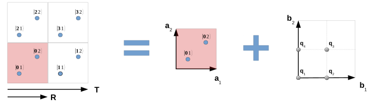
Figure 1: Schematic representation of the supercell — primitive cell mapping in 2D. A $2\times 2$ supercell problem with a $\Gamma$ only sampling can be recast in a primitive cell problem with a $2\times 2$ sampling of the Brillouin zone.

The first step in this reformulation is to rewrite the Wannier orbital densities as Bloch sums in the primitive cell. A schematic view of the supercell-primitive cell mapping is shown in Fig. 1. Using the definition of the MLWFs, the Wannier orbital densities can be written as

$$\rho_{{\bf R}n}({\bf r}) =|\omega_{{\bf R}n}({\bf r})|^{2}=\left|\frac{1}{N_{{\bf k}}}\sum_{{\bf k}}e^{-i{\bf k}\cdot{\bf R}}\tilde{\psi}_{{\bf k}n}({\bf r})\right|^{2}$$

$$=\frac{1}{N_{{\bf q}}}\sum_{{\bf q}}e^{i{\bf q}\cdot{\bf r}}\left\{e^{-i{\bf q}\cdot{\bf R}}\frac{1}{N_{{\bf k}}}\sum_{{\bf k}}w^{*}_{{\bf k},n}({\bf r})w_{{\bf k}+{\bf q},n}({\bf r})\right\}$$

$$=\frac{1}{N_{{\bf q}}}\sum_{{\bf q}}e^{i{\bf q}\cdot{\bf r}}\rho_{{\bf q}}^{{\bf R}n}({\bf r}).$$ (11)

Since the $w_{{\bf k}n}({\bf r})$ are periodic on the primitive cell, the $\rho^{{\bf R}n}_{{\bf q}}({\bf r})$ are also, and consequently the Wannier orbital density is given as a sum over the Brillouin zone (BZ) of primitive cell-periodic function just modulated by a phase factor $e^{i{\bf q}\cdot{\bf r}}$. The periodic densities $\rho^{{\bf R}n}_{{\bf q}}({\bf r})=\rho^{{\bf R}n}_{{\bf q}}({\bf r}+{\bf R})$ are the basic ingredients needed to express integrals over the supercell appearing in the definitions of the screening coefficients and of the KI corrections and potentials into integrals over the primitive cell.

3.1.1 Screening coefficients

The expression for the screening coefficients given in Eq. (6) can be recast in a linear response-problem ⁶⁰ suitable for an efficient implementation based on DFPT ⁸⁷:

$$\alpha_{{\mathbf{0}}n} =\frac{\langle\rho_{{\mathbf{0}}n}|\left[\epsilon^{-1}f_{\rm Hxc}\right]|\rho_{{\mathbf{0}}n}\rangle}{\langle\rho_{{\mathbf{0}}n}|\left[f_{\rm Hxc}\right]|\rho_{{\mathbf{0}}n}\rangle}=1+\frac{\langle V^{{\mathbf{0}}n}_{\rm pert}|\Delta^{{\mathbf{0}}n}\rho\rangle}{\langle\rho_{{\mathbf{0}}n}|V^{{\mathbf{0}}n}_{\rm pert}\rangle}.$$ (12)

In the expression above we made use of the definition of the dielectric matrix $\epsilon^{-1}=1+f_{\rm Hxc}\chi$ with $\chi$ being the density-density response function of the system at the underlying DFT level; $\Delta^{{\mathbf{0}}n}\rho({\bf r})=\int d{\bf r}^{\prime}\chi({\bf r},{\bf r}^{\prime})V_{\rm pert}^{{\mathbf{0}}n}({\bf r}^{\prime})$ is by definition the density response induced in the systems due to the “perturbing potential” $V^{{\mathbf{0}}n}_{\rm pert}({\bf r})=\int d{\bf r}^{\prime}f_{\rm Hxc}({\bf r},{\bf r}^{\prime})\rho_{n}({\bf r}^{\prime})$. This perturbation represents the Hartree-exchange-correlation potential generated when an infinitesimal fraction of an electron is added to/removed from a MLWF. The perturbing potential has the same periodic structure as the Wannier density in Eq. (11) and can be decomposed into a sum of monochromatic perturbations in the primitive cell, $V_{\rm pert}^{{\mathbf{0}}n}({\bf r})=\sum_{{\bf q}}e^{i{\bf q}\cdot{\bf r}}V^{{\mathbf{0}}n}_{{\rm pert},{\bf q}}({\bf r})$ with

$$V^{{\mathbf{0}}n}_{{\rm pert},{\bf q}}({\bf r})=\int d{\bf r}^{\prime}f_{\rm Hxc}({\bf r},{\bf r}^{\prime})\rho^{{\mathbf{0}}n}_{{\bf q}}({\bf r}^{\prime}).$$ (13)

The total density variation $\Delta^{{\mathbf{0}}n}\rho({\bf r}^{\prime})$ induced by the bare perturbation $V_{\rm pert}^{{\mathbf{0}}n}({\bf r})$ reads

$$\Delta^{{\mathbf{0}}n}\rho({\bf r}) =\int d{\bf r}^{\prime}\chi({\bf r},{\bf r}^{\prime})V_{\rm pert}^{{\mathbf{0}}n}({\bf r}^{\prime})$$

$$=\int d{\bf r}^{\prime}\chi({\bf r},{\bf r}^{\prime})\sum_{{\bf q}}e^{i{\bf q}\cdot{\bf r}^{\prime}}V_{{\rm pert},{\bf q}}^{{\mathbf{0}}n}({\bf r}^{\prime})$$

$$=\sum_{{\bf q}}e^{i{\bf q}\cdot{\bf r}}\Delta_{{\bf q}}^{{\mathbf{0}}n}\rho({\bf r})$$ (14)

where we used the fact that for a periodic system $\chi$ can be decomposed in a sum of primitive cell-periodic functions $\chi({\bf r},{\bf r}^{\prime})=\sum_{{\bf q}}e^{i{\bf q}\cdot({\bf r}-{\bf r}^{\prime})}\chi_{{\bf q}}({\bf r},{\bf r}^{\prime})$  . The primitive cell-periodic density variation is given by:

$$\Delta_{{\bf q}}^{{\mathbf{0}}n}\rho({\bf r}) =\int d{\bf r}^{\prime}\chi_{{\bf q}}({\bf r},{\bf r}^{\prime})V_{{\rm pert},{\bf q}}^{{\mathbf{0}}n}({\bf r}^{\prime})$$

$$=\sum_{{\bf k}v}\psi_{{\bf k},v}^{*}({\bf r})\Delta\psi_{{\bf k}+{\bf q},v}({\bf r})+c.c.$$ (15)

where $\Delta\psi_{{\bf k}+{\bf q}}({\bf r})$ is the first order variation of the KS orbitals due to the perturbation (the bare one plus the SCF response in the Hxc potential). Only the projection of the variation of the KS wave functions on the conduction manifold contributes to the density response in Eq. (15), meaning that $\Delta\psi_{{\bf k}+{\bf q}}({\bf r})$ can be thought of as its own projection on this manifold and it is given by the solution of the following linear problem ⁸⁷:

$$\left(H+\gamma P_{v}^{{\bf k}+{\bf q}}-\varepsilon_{{\bf k},v}\right)\Delta\psi_{{\bf k}+{\bf q},v}({\bf r})$$

$$= -P_{c}^{{\bf k}+{\bf q}}\left[V_{{\rm pert},{\bf q}}^{{\mathbf{0}}n}({\bf r})+\Delta_{{\bf q}}V_{\rm Hxc}({\bf r})\right]\psi_{{\bf k},v}({\bf r})$$ (16)

where $H$ is the ground state KS Hamiltonian, $P_{v}^{{\bf k}}=\sum_{v}|u_{{\bf k},v}\rangle\langle u_{{\bf k},v}|$ and $P_{c}^{{\bf k}}=1-P_{v}^{{\bf k}}$ are the projectors onto the occupied- and empty-manifold respectively, $\gamma$ is a constant chosen in such a way that the $\gamma P_{v}^{{\bf k}+{\bf q}}$ operator makes the linear system non-singular ⁸⁷, and

$$\Delta_{{\bf q}}V_{\rm Hxc}({\bf r})=\int d{\bf r}^{\prime}f_{\rm Hxc}({\bf r},{\bf r}^{\prime})\Delta^{{\mathbf{0}}n}_{{\bf q}}\rho({\bf r}^{\prime})$$ (17)

is the self-consistent variation of the Hxc potential due to the charge density variation $\Delta_{{\bf q}}^{{\mathbf{0}}n}\rho$. Iterating Eqs. (15)-(17) to self-consistency leads to the final results for $\Delta\rho_{{\bf q}}^{{\mathbf{0}}n}({\bf r})$ and the screening coefficient is finally obtained by summing over all the ${\bf q}$ contributions:

$$\alpha_{{\mathbf{0}}n}=1+\frac{\sum_{{\bf q}}\langle V^{{\mathbf{0}}n}_{{\rm pert},{\bf q}}|\Delta^{{\mathbf{0}}n}_{{\bf q}}\rho\rangle}{\sum_{{\bf q}}\langle{\rho^{{\mathbf{0}}n}_{{\bf q}}}|V^{{\mathbf{0}}n}_{{\rm pert},{\bf q}}\rangle}.$$ (18)

Equations  (13)-(17) show how to recast the calculation of the screening coefficient into a linear response problem in the primitive cell that can be efficiently solved using the machinery of DFPT ,and are key to the present work. Linear-response equations for different ${\bf q}$ are decoupled and the original problem is thus decomposed into a set of independent problems that can be solved on separate computational resources, allowing for straightforward parallelization. More importantly, the computational cost is also greatly reduced: In a standard supercell implementation the screening coefficients are computed with a finite difference approach by performing additional total-energy calculations where the occupation of a Wannier function is constrained ²⁶. This requires, for each MLWF, multiple SCF calculations with a computational time $T^{\rm SC}$ that scales roughly as ${N_{\rm el}^{\rm SC}}^{3}$, where $N_{\rm el}^{\rm SC}$ is the number of electrons in the supercell. The primitive cell DFPT approach described above scales instead as $T^{\rm PC}\propto N_{{\bf q}}N_{{\bf k}}{N_{\rm el}^{\rm PC}}^{3}$; this is the typical computational time for the SCF cycle ($N_{{\bf k}}{N_{\rm el}^{\rm PC}}^{3}$), times the number of independent monochromatic perturbations ($N_{{\bf q}}$). Using the relation $N_{\rm el}^{\rm SC}=N_{{\bf k}}N_{\rm el}^{\rm PC}$, and the fact that $N_{{\bf q}}=N_{{\bf k}}$, the ratio between the supercell and primitive cell computational times is $T^{\rm SC}/T^{\rm PC}\propto N_{{\bf q}}$. Therefore as the supercell size (and, equivalently, the number of ${\bf q}$-points in the primitive cell) increases, the primitive cell DFPT approach becomes more and more computationally convenient. We finally point out that a similar strategy was recently implemented in the context of the linear-response approach to the calculation of the Hubbard parameters in DFT+U ³⁰ in order to avoid the use of a supercell ^{88, 89}.

3.1.2 KI Hamiltonian

As it is typical for orbital-density-dependent functionals, the canonical eigenvalues and eigenvectors are given by the diagonalization of the matrix of Lagrangian multipliers $H_{mn}({\bf R})=\langle{\bf R}m|\hat{h}_{{\mathbf{0}}n}|{\mathbf{0}}n\rangle$ with $\hat{h}_{{\mathbf{0}}m}|{\mathbf{0}}n\rangle=\delta E^{\rm KI(2)}/\delta\langle{\bf R}n|$. In the case of insulating systems, the matrix elements between occupied and empty states vanish ²³ and we can treat the two manifolds separately. For occupied states, the KI potential is simply a scalar correction (the second term in Eq. (9) is identically zero if $f_{i}=1$), and thus the KI contribution to the Hamiltonian is diagonal and ${\bf R}$-independent:

$$\Delta H^{\rm KI(2)}_{vv^{\prime}}({\bf R}) =\langle{\bf R}v|\mathcal{V}^{\rm KI(2)}_{{\mathbf{0}}v^{\prime}}|{\mathbf{0}}v^{\prime}\rangle$$

$$=-\frac{1}{2N_{{\bf q}}}\sum_{{\bf q}}\langle{\rho^{{\mathbf{0}}v}_{{\bf q}}}|V^{{\mathbf{0}}v}_{{\rm pert},{\bf q}}\rangle\delta_{{\bf R},{\mathbf{0}}}\delta_{vv^{\prime}}$$

$$=-\frac{1}{2}\Delta^{\rm KI(2)}_{{\mathbf{0}}v}\delta_{{\bf R},{\mathbf{0}}}\delta_{vv^{\prime}}$$ (19)

Using the definition of $|{\bf R}v\rangle$ or equivalently the identity $\delta_{{\bf R},{\mathbf{0}}}=1/N_{{\bf k}}\sum_{{\bf k}}e^{i{\bf k}\cdot{\bf R}}$ in the equation above, the KI contribution to the Hamiltonian at a given ${\bf k}$ can be identified as:

$$\Delta H^{\rm KI(2)}_{vv^{\prime}}({\bf k}) =-\frac{1}{2}\Delta^{\rm KI(2)}_{{\mathbf{0}}v}\delta_{vv^{\prime}}$$ (20)

which is ${\bf k}$-independent, as expected.

In the case of empty states, in addition to the scalar term in the equation above, there is also a non-scalar contribution ²⁴ that needs a more careful analysis. This term is given by the matrix element of the non-scalar contribution to the KI potential, i.e. $\mathcal{V}^{\rm KI(2),r}_{{\mathbf{0}}c}({\bf r})=\int d{\bf r}^{\prime}f_{\rm Hxc}({\bf r},{\bf r}^{\prime})\rho_{{\mathbf{0}}c}({\bf r}^{\prime})$, and reads:

$$\Delta H^{\rm KI(2),r}_{cc^{\prime}}({\bf R}) =\langle{\bf R}c|\mathcal{V}^{\rm KI(2),r}_{{\mathbf{0}}c^{\prime}}|{\mathbf{0}}c^{\prime}\rangle$$

$$=\frac{1}{N_{{\bf k}}}\sum_{{\bf k}}e^{i{\bf k}\cdot{\bf R}}\left[\frac{1}{N_{{\bf q}}}\sum_{{\bf q}}\langle V^{{\mathbf{0}}c^{\prime}}_{{\rm pert},{\bf q}}|\rho^{cc^{\prime}}_{{\bf k},{\bf k}+{\bf q}}\rangle\right]$$ (21)

where $\rho^{cc^{\prime}}_{{\bf k},{\bf k}+{\bf q}}({\bf r})=w^{*}_{{\bf k},c}({\bf r})w_{{\bf k}+{\bf q},c^{\prime}}({\bf r})$ (see Supporting Information for a detailed derivation of the KI matrix elements). Since the dependence on the ${\bf R}$-vector only appears in the complex exponential, the matrix elements of the KI Hamiltonian in ${\bf k}$-space can be easily identified as the term inside the square brackets in Eq.(21). Including the scalar contribution leads to the ${\bf k}$-space Hamiltonian for the empty manifold:

$$\Delta H^{\rm KI(2)}_{cc^{\prime}}({\bf k})=-\frac{1}{2}\Delta^{\rm KI(2)}_{{\mathbf{0}}c}\delta_{cc^{\prime}}+\frac{1}{N_{{\bf q}}}\sum_{{\bf q}}\langle V^{{\mathbf{0}}c^{\prime}}_{{\rm pert},{\bf q}}|\rho^{cc^{\prime}}_{{\bf k},{\bf k}+{\bf q}}\rangle$$ (22)

Eqs. (20) and (22) define the KI contribution to the Hamiltonian at a given ${\bf k}$ point on the regular mesh used for the sampling of the Brillouin zone. This contribution needs to be scaled by the screening coefficient $\alpha_{{\mathbf{0}}n}$ and added to the DFT Hamiltonian to define the full KI Hamiltonian at ${\bf k}$ as:

$$H^{\rm KI(2)}_{mn}({\bf k})=H^{\rm DFT}_{mn}({\bf k})+\alpha_{{\mathbf{0}}n}\Delta H^{\rm KI(2)}_{mn}({\bf k})$$ (23)

where $H^{\rm DFT}_{mn}({\bf k})=\langle w_{{\bf k}m}|\hat{H}^{\rm DFT}|w_{{\bf k}n}\rangle$ is the KS-DFT Hamiltonian evaluated on the periodic part of the Bloch states in the Wannier gauge (see Eq. (10)). The diagonalization of $H^{\rm KI(2)}_{mn}({\bf k})$ defines the canonical KI eigenstates $\{\psi_{{\bf k}i}^{\rm KI(2)};\varepsilon_{{\bf k}i}^{\rm KI(2)}\}$. Finally, given the localized nature of the MLWFs it is also possible to interpolate the Hamiltonian with standard techniques ^{90, 91, 65} to obtain the KI eigenvalues at any arbitrary ${\bf k}$ point in the Brillouin zone.

3.2 Technical aspects of the implementation

The calculations of the screening parameters and KI potentials involve the evaluation of bare and screened Hxc integrals of the form $\langle\rho_{{\mathbf{0}}n}|f_{\rm Hxc}|\rho_{{\mathbf{0}}n}\rangle$ and $\langle\rho_{{\mathbf{0}}n}|\epsilon^{-1}f_{\rm Hxc}|\rho_{{\mathbf{0}}n}\rangle$. Because of the long-range nature of the Hartree kernel, these integrals are diverging in periodic-boundary conditions (PBC) and therefore require particular caution. The divergence can be avoided adding a neutralizing background (in practice this means that the ${\bf q}+{\bf G}={\mathbf{0}}$ component of the Hartree kernel is always set to zero). The integrals are then finite and, more importantly, converge to the correct electrostatic energy of isolated Wannier functions. ⁹² However, the convergence is extremely slow ($1/N_{{\bf k}}^{1/3}$ to leading order) because of the $1/|{\bf q}+{\bf G}|^{2}$ divergence in the Coulomb kernel. This is a well know problem and many solutions have been proposed to overcome it; e.g. Makov and Payne ⁹² (MP) suggested to remove from the energy the electrostatic interaction of a periodically-repeated point-charge. Other approaches consist in truncating the Coulomb interaction ^{93, 94} or using the scheme proposed by Martyna and Tuckermann ⁹⁵ or the charge or density corrections of Ref. 96. Here we adopt the approach devised by Gygi and Baldereschi (GB) ⁹⁷ that consists of adding and subtracting to the integrand a function with the same divergence and whose integral can be computed analytically. The result is a smooth function suitable for numerical integration, plus an analytical contribution. From a computational point of view this amounts to defining a modified Hartree kernel

$$f_{\rm H}({\bf q}+{\bf G})=\begin{cases}D,&\text{if }{\bf q}+{\bf G}={\mathbf{0}}\\ 4\pi/|{\bf q}+{\bf G}|^{2},&\text{if }{\bf q}+{\bf G}\neq{\mathbf{0}}\end{cases}$$ (24)

where $D$ is the reciprocal-space part of the Ewald sum for a point charge, repeated according to the super-periodicity defined by the grid of ${\bf q}$-points ⁹⁸. For the screened Hartree integral the ${\bf q}+{\bf G}=0$ component needs to be further scaled by the macroscopic dielectric function $\epsilon_{\infty}$ of the system  because in this case we are dealing with the screened Coulomb integral $\epsilon^{-1}f_{H}$. In this work we compute $\epsilon_{\infty}$ from first-principles ⁸⁷ using the PHONON code of Quantum ESPRESSO .

Another important point is that the periodic part of the Wannier function at ${\bf k}$ and ${\bf k}+{\bf q}$ must come from the same Wannierization procedure, otherwise the localization property of the Wannier orbital density [Eq. (11)] will be lost because of unphysical phase factors possibly due to the diagonalization routine or other computational reasons. This requirement is enforced using a uniform grid centered at $\Gamma$ such that ${\bf k}+{\bf q}={\bf p}+{\bf G}$ with ${\bf p}$ still belonging to the original grid and ${\bf G}$ a reciprocal lattice vector. In this way $w_{{\bf k}+{\bf q}}({\bf r})$ can be obtained from $w_{{\bf p}}({\bf r})$ simply multiplying it by a phase factor $e^{-i{\bf G}\cdot{\bf r}}$. As a direct consequence of this choice the mesh of ${\bf q}$ points for the LR calculation has to be the same as the one used for the Wannierization.

Finally, in order to be compliant with the current limitation of working with block-diagonal occupation matrices (see. Sec. 2.2.3), the Wannierization procedure needs to be prevented from mixing the occupied and empty manifolds, so that the occupation matrix retains its block-diagonal form in the localized-orbital representation. In practice this is done by performing two separate Wannierizations, one for the occupied and one for the empty manifold. To obtain the maximally localized Wannier orbitals for the low-lying empty states, we employed the disentanglement maximally localized Wannier function technique proposed in Ref. 91.

Sys.	wann	method	$\frac{\partial^{2}E}{\partial f^{2}}[eV]$	$\frac{d^{2}E}{df^{2}}[eV]$	$\alpha$
Si	$sp^{3}$ (V)	FD	3.906	0.888	0.227
		DFPT	3.886	0.887	0.228
	$sp^{3}$ (C)	FD	1.351	0.215	0.160
		DFPT	1.351	0.218	0.162
GaAs	$d$ (V)	FD	10.159	3.530	0.347
		DFPT	10.217	3.550	0.347
	$sp^{3}$ (V)	FD	3.899	0.976	0.250
		DFPT	3.896	0.936	0.240
	$sp^{3}$ (C)	FD	1.418	0.233	0.164
		DFPT	1.372	0.243	0.177

Table 1: Comparison between analytical (computed with DFPT) and numerical [computed with finite differences (FD)] second derivatives of the energy with respect to the occupation of different kinds of Wannier functions for silicon (Si) and gallium arsenide (GaAs). V / C indicates whether the MLWF is from the valence or conduction manifold. Partial $\partial/\partial f_{i}$ and full $d/df_{i}$ derivatives refer to unrelaxed and relaxed quantity, respectively.

4 Results and discussion

In this section we first validate the present implementation against a standard KI one as described in Ref. 26, and then discuss the application to few paradigmatic test cases, highlighting the advantages and limitations of the approach. In particular we analyze the band structure of gallium arsenide (GaAs), hexagonal wurtzite zinc oxide (ZnO) and face-centered-cubic (FCC) lithium fluoride (LiF) at three levels of theory: i) the local density approxination (LDA), ii) the hybrid-functional scheme by Heyd Scuseria and Ernzerhof (HSE) ^{102, 103}, and iii) the KI functional within the implementation described in this work. All calculations are performed using the plane-wave (PW) and pseudopotential (PP) method as implemented in the Quantum ESPRESSO  package ^{104, 105}. The LDA functional is used as the underlying density-functinal approximation for all the KI calculations. LDA scalar relativistic Optimized Norm-conserving Vanderbilt PPs ^{106, 107} from the DOJO library ¹⁰⁸ are used to model the interaction between the valence electrons and the nucleus plus the core electrons . Maximally localized Wannier functions are computed using the Wannier90 code ¹⁰⁹. For all the systems we used the experimental crystal structures taken from the inorganic Crystal Structure Database  (ICSD); GaAs, ZnO and LiF correspond to ICSD numbers 107946, 162843 and 62361 respectively. For the LDA calculations we used a $10\times 10\times 10$ ${\bf k}$-point mesh for GaAs, a $12\times 12\times 7$ ${\bf k}$-point mesh for ZnO and a $14\times 14\times 14$ ${\bf k}$-point mesh for LiF. The kinetic energy cutoff for the PW expansion of the wave-functions is set to $E_{\rm cut}=80$ Ry (320 Ry for the density and potentials expansion) in all cases. For the HSE calculations we verified that a reduced cutoff $E^{\rm Fock}_{\rm cut}=120$ and a ${\bf k}$-point grid typically twice as coarse as the LDA one are sufficient for the convergence of the exchange energy and potential. For the screening parameters and KI Hamiltonian calculations we used the same energy cutoff and a ${\bf q}$-mesh of $6\times 6\times 6$ for GaAs and LiF, and a $6\times 6\times 4$ mesh for ZnO.

Figure 2: KI density of states of Si (upper panel) and GaAs (lower panel) computed with a reference 4$\times$4$\times$4 supercell (red line) and with the present approach working in the primitive cell with a commensurate 4$\times$4$\times$4 ${\bf k}$-points mesh.

GaAs band structure

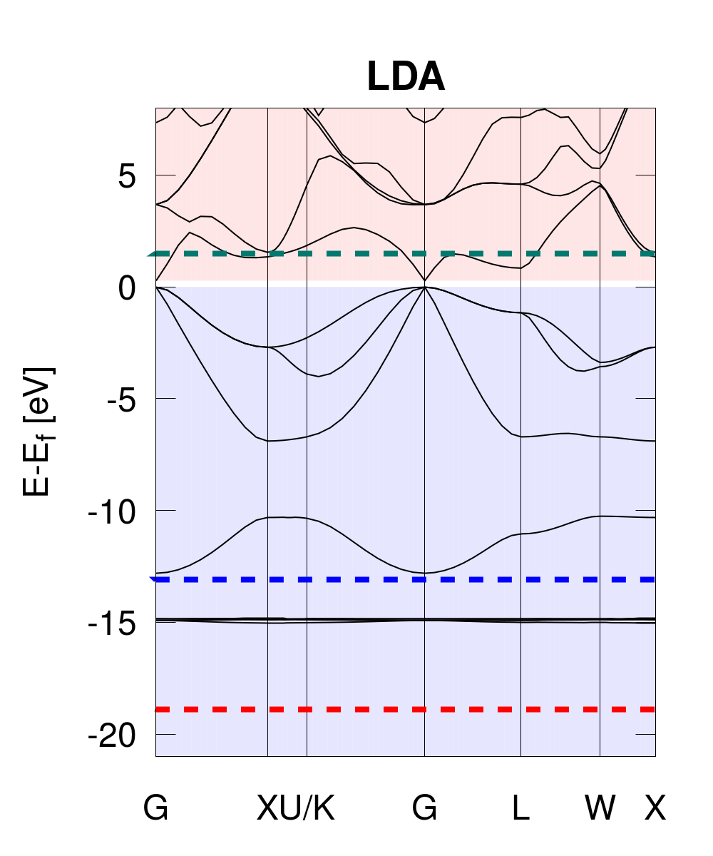
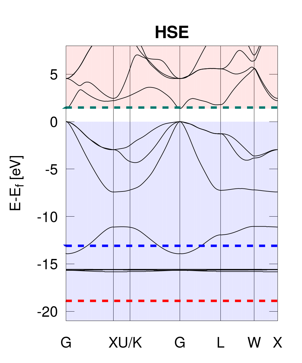
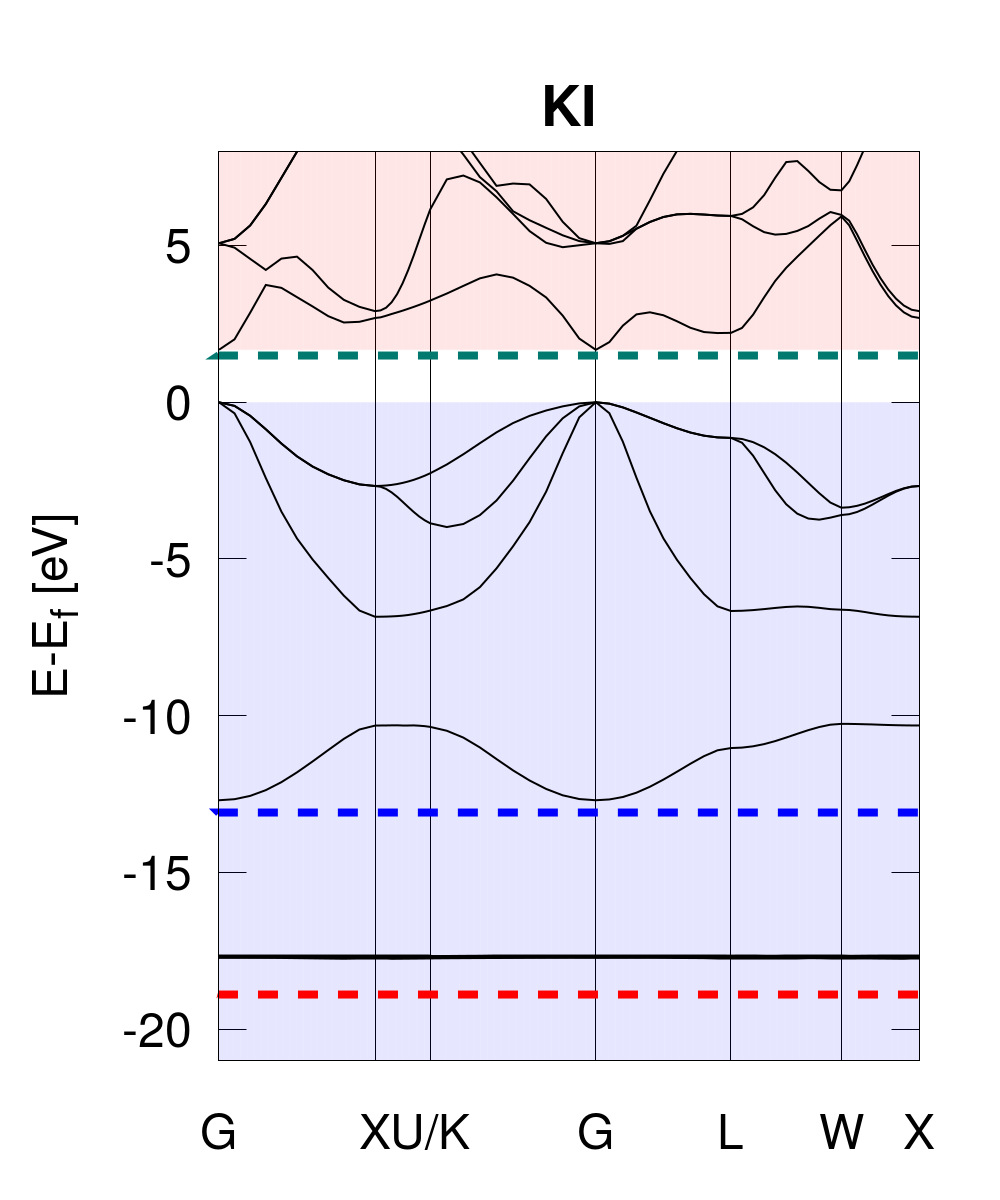
	LDA	HSE	GW0	scG$\tilde{\rm W}$	KI	Exp.
Egap(eV)	0.19	1.28	1.55	1.62	1.57	1.52
$\langle\varepsilon_{d}\rangle$(eV)	-14.9	-15.6	-17.3	-17.6	-17.7	-18.9
$W$(eV)	12.8	13.9	–	–	12.8	13.1

Figure 3: Band structure of GaAs calculated at different levels of theory: LDA (left panel), HSE (middle panel) and KI (right panel). Shaded areas highlight valence (light blue) and conduction (light red) manifolds. The experimental values for the band gap, valence band width, and energy position of Ga $d$-states are represented by the dashed green, blue and red lines, respectively. Table: Band gap, position of Ga $d$ states with respect to the top of the valence band, and valence band width ($W$) at different level of theory compared to experimental ^{110, 111} and GW results from Ref. 112. Theoretical values of the band gap are corrected for spin-orbit coupling (0.10 eV).

4.1 Validation

In order to validate the implementation of the analytical formula for the derivatives based on the DFTP [Eq. (12)], we compare the result with a finite difference calculation where we add/remove a tiny fraction of an electron from a given Wannier function. This is done using a 4$\times$4$\times$4 supercell, consistent with the ${\bf k}$/${\bf q}$ mesh in the primitive cell calculation. In Table (1) we present the results for two semiconductors, silicon (Si) and gallium arsenide (GaAs). For Si the Wannierization produces four identical bonding $sp^{3}$-like MLWFs spanning the occupied manifold and four anti-bonding $sp^{3}$-like MLWFs spanning a four-dimensional manifold disentangled from the lowest part of the conduction bands. In the case of GaAs we obtained 5 $d$-like and 4 $sp^{3}$-like MLWFs representing the occupied manifold and 4 anti-bonding $sp^{3}$-like MLWFs from the lowest part of the empty manifold. The numerical and analytical values for the derivatives agree within few hundredths of an eV. The residual discrepancy is possibly due to tiny differences in the Wannierization procedure (for the supercell a specific algorithm for a $\Gamma$-only calculation was used), and to the difficulties in converging to arbitrary accuracy the constrained calculations in the supercell.

In order to quantify the error introduced by the second-order approximation adopted here, we compare in Fig. (2) the KI density of states for Si and GaAs computed using a 4$\times$4$\times$4 supercell within the original implementation ^{26, 61}, and the present approach working in primitive cell with a consistent 4$\times$4$\times$4 ${\bf k}/{\bf q}$-points mesh. For this figure the single particle eigenvalues were convoluted with a Gaussian function with a broadening of 0.2 eV. The zero of the energy is set to the LDA valence band maximum (VBM), and the shaded red area represent the LDA band gap. The thick black ticks on the energy axes mark the position of the KI VBM and conduction band minimum (CBM). The KI VBM and CBM are shifted downwards and upwards with respect to the corresponding LDA quantities, leading to an opening the fundamental band gap, that goes from 0.51 eV to 1.41 eV and from 0.20 eV to 1.57 eV for Si and GaAs, respectively. We stress here that these results are not fully converged with respect to the BZ sampling (or supercell size), and serve just as a validation test. The two DOS are in very good agreement, but small differences between the reference supercell and the primitive cell calculations are present. In particular there is a small downward shift of the order or 0.05 eV in the valence part of the DOS, and also tiny differences in the conduction one, especially evident for GaAs. These discrepancies are due to the second order approximation used for the calculation of the screening parameters and KI Hamiltonian in the primitive cell implementation (additional details are provided in Supporting Information). Nevertheless, all the main features of the DOS are correctly reproduced, thus validating the present implementation.

4.2 Application to selected systems

Gallium arsenide: GaAs is a III-V direct band gap semiconductor with a zincblende crystal structure. The band structure around the band gap is dominated by $s$ and $p$ orbitals from Ga and As forming $sp^{3}$ hybrid orbitals while the flat bands around 18.9 eV below the VBM are from the $d$ states of Ga. All these features are correctly reproduced by the LDA band structure [see Fig. (3)] but the band gap $E^{\rm LDA}_{\rm gap}=0.28$ eV is too small, the average $d$ states position $\langle\varepsilon^{\rm LDA}_{d}\rangle=-14.9$ eV is too high, and the valence bad width $W^{\rm LDA}=12.8$ eV is slightly underestimated. The HSE functional corrects these errors to some extent, opening the band gap up to $E^{\rm HSE}_{\rm gap}=1.38$ eV, and shifting downwards the Ga $d$ states, $\langle\varepsilon^{\rm HSE}_{d}\rangle=-15.6$ eV, but it also over-stretches the valence band thus overestimating the valence band width ($W^{\rm HSE}=13.9$ eV). These discrepancies with respect to experiment are possibly due to the fact that the fraction of Fock exchange and the range-separation parameter defining any hybrid scheme might have to be in principle system- and possibly state-dependent ^{49, 50, 113}. On the contrary the parameters of the HSE functionals (and also of the vast majority of hybrid schemes) are system-independent and this is probably not sufficient for an accurate description of all the spectral features mentioned above. The KI functional with its orbital-dependent corrections produces an upward shift of the conduction manifold and a state-dependent downward shift of the valence manifold (with respect to the LDA VBM), leading to a better agreement with experimental data for $E_{\rm gap}$ and $\langle\varepsilon_{d}\rangle$. The $sp^{3}$ band width is instead identical to that of the underlying density functional approximation (LDA), which is already in good agreement with the experimental value. This is because of the scalar nature of the KI corrections for the occupied manifold combined with the fact that the Wannierization produces four identical but differently-oriented $sp^{3}$ MLWFs spanning the four uppermost valence bands. Then from Eq. (20) it follows that the KI contribution to the Hamiltonian is not only ${\bf k}$-independent but also the same for all the $sp^{3}$ bands. The KIPZ functional ²⁴, another flavor of KC functionals, might correct this because of its non-scalar contribution to the effective potentials. This will introduce an off-diagonal coupling between different bands and will thus modify the band width ⁶¹. Overall the KI results are in extremely good agreement with experimental data. This performance is even more remarkable if compared to GW results ¹¹² reported in the Table under Fig. 3, with KI showing the same accuracy as self-consistent GW plus vertex correction in the screened Coulomb interaction.

LiF band structure

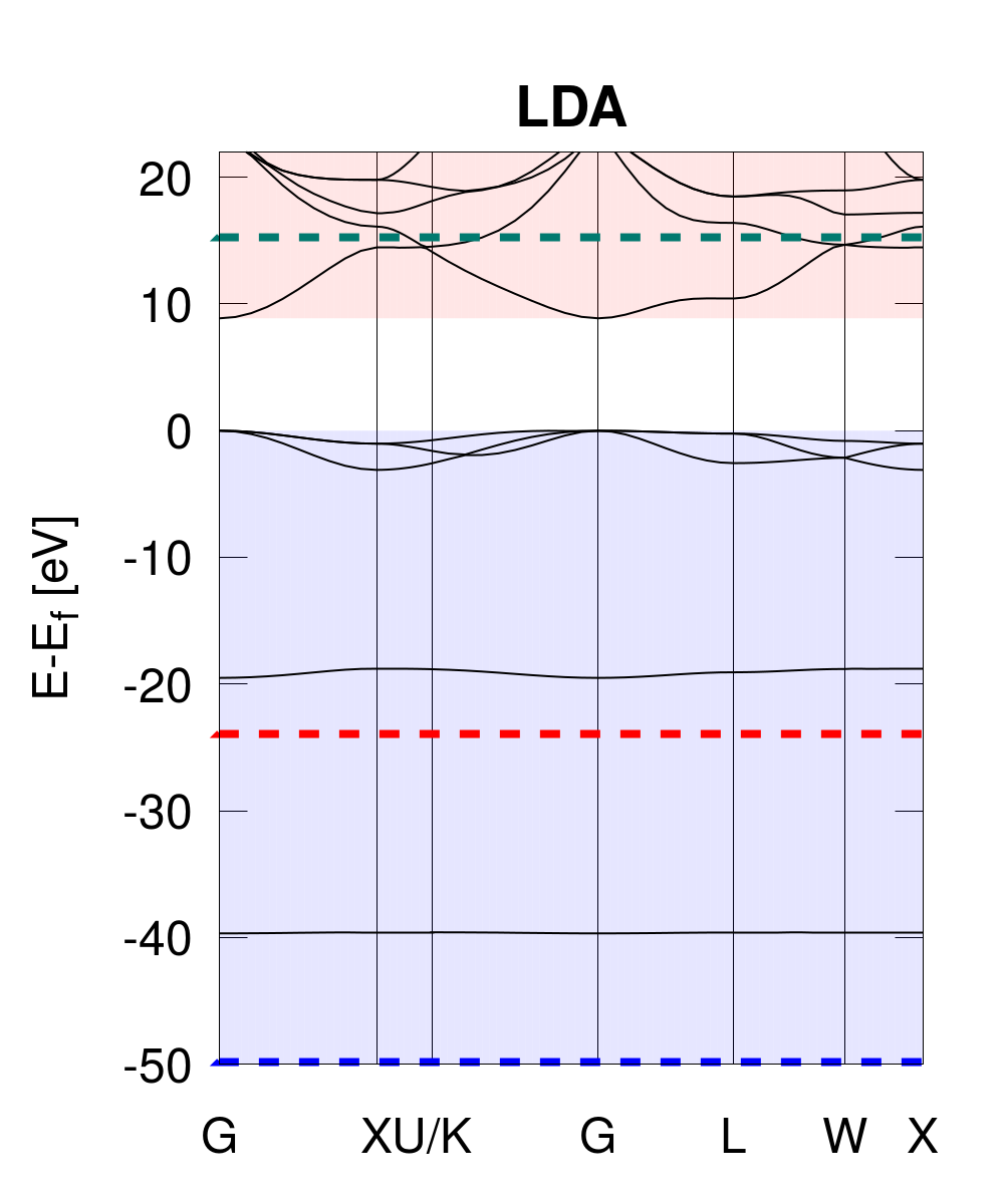
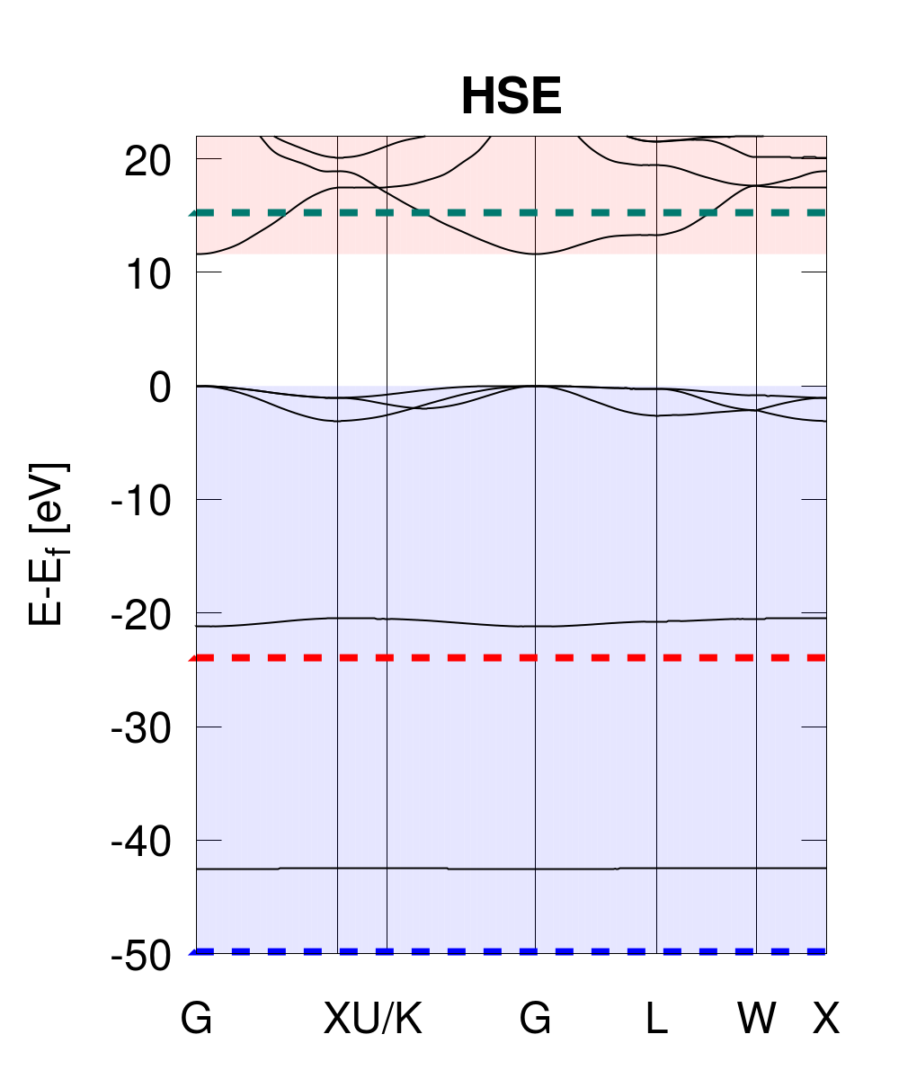
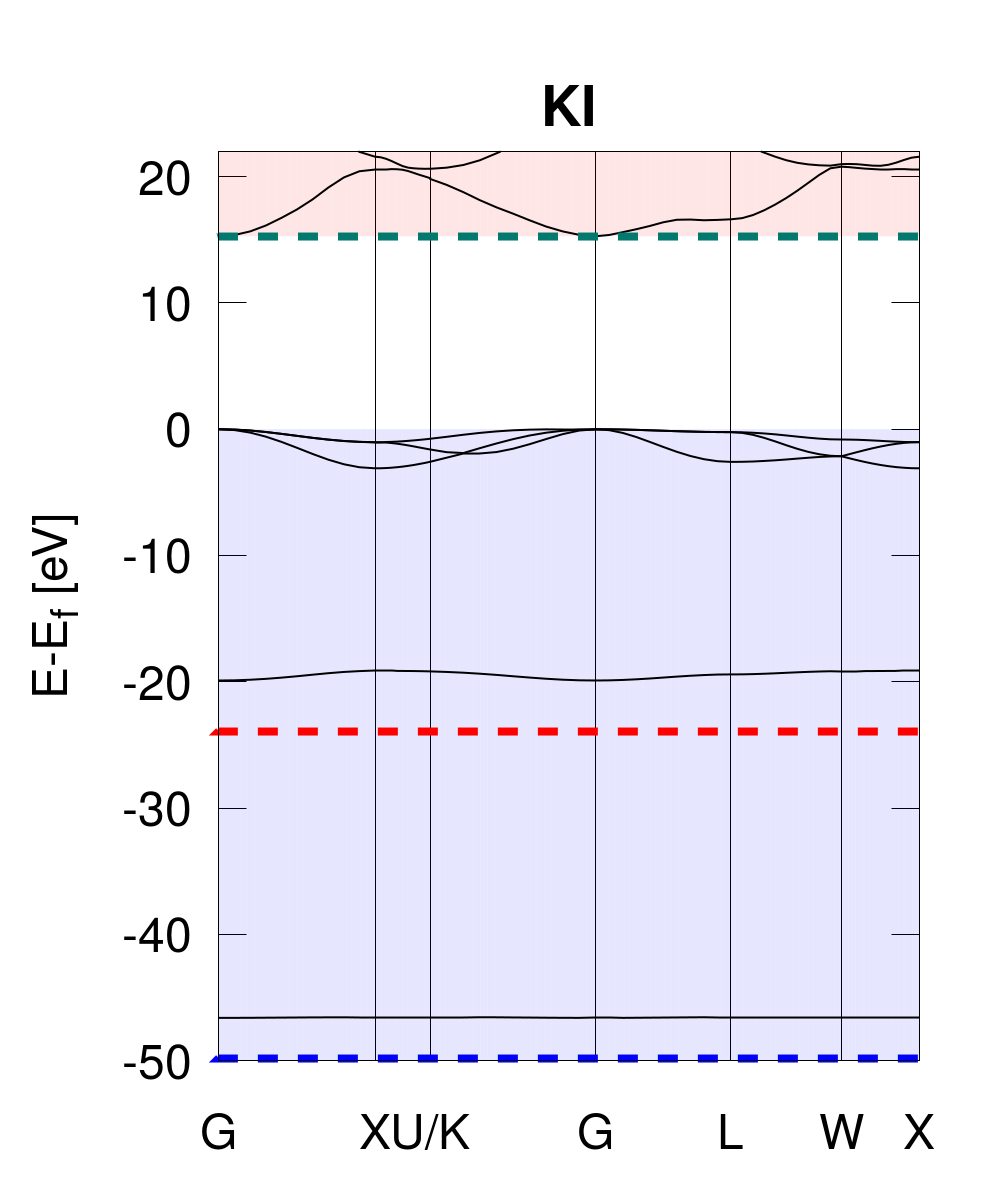
	LDA	HSE	GW0	scG$\tilde{\rm W}$	KI	(Exp.)
Egap(eV)	8.87	11.61	13.96	14.5	15.28	15.35(∗)
$\langle\varepsilon\rangle_{\rm{F}_{2s}}$(eV)	-19.06	-20.7	-24.8(†)	–	-19.5	-23.9
$\langle\varepsilon\rangle_{\rm{Li}_{1s}}$(eV)	-39.6	-42.5	-47.2(†)	–	-46.6	-49.8

Figure 4: Band structure of LiF calculated at different levels of theory: LDA (left panel), HSE (middle panel) and KI (right panel). Shaded areas highlight valence (light blue) and conduction (light red) manifolds. The experimental value for the band gap, the F $2s$ band and Li $1s$ band are represented by the dashed green, red, and blue lines, respectively. Table: Band gap and low lying energy levels at different levels of theory compared to GW results ^{112, 114, 115} and to experiments ^{116, 117}. ^(∗) The zero-point-renormalization ¹¹⁸ (-1.15 eV) has been subtracted to the experimental gap ¹¹⁶ (14.2 eV) to have a meaningful comparison with the calculations. $(^{\dagger})$ Values obtained at G₀W₀ level. ¹¹⁵

Lithium fluoride: LiF crystallizes in a rock-salt structure and provides a prototypical example of wide gap insulators with a marked ionic character. Its band structure at all the different levels of theory analyzed in this work is presented in Fig. (4). LiF is a direct band gap material with the topmost valence bands exclusively contributed by F $2p$ orbitals, and the lower part of the conduction manifolds mainly from Li $2s$ orbitals with a small contribution from F $2p$ orbitals. The low lying energy levels at about -24 eV and -50 eV with respect to the top of the valence bands can be unambiguously classified as F $2s$ and Li $1s$ bands, respectively. Also in this case we observe all the limitations of LDA already observed and discussed for GaAs and the same trend going from local to hybrid to orbital-density dependent KI functionals. In particular, the KI band gap is in very good agreement with the experimental band gap ¹¹⁶ after the zero point renormalization energy ¹¹⁸ is added to have a fair comparison between calculations (no electron-phonon effects are accounted for) and experiments. Thanks to the state-dependent potentials the Li $1s$ band is pushed downwards in energy more than the valence bands are, and its relative position with respect to the VBM results in a much better agreement with experimental values. On the other hand the F_2s band is shifted downwards in energy by roughly the same amount as the three valence bands (originating from the F_2p states) are. This leaves almost unchanged its distance with respect to the VBM ( 19.5 eV at KI level compared to -19.06 at LDA level). This is at odd with GW results ¹¹⁵ which show an increase in the relative distance of roughly 5 eV and place the F_2s band at -24.8 eV with respect to the VBM, in better agreement with experimental results ¹¹⁷(-23.9 eV). Full KI and KIPZ band structures show the same underestimation although less severe (see Supporting Information), especially when using a better underlying density functional (PBE vs LDA). This seems to suggest this underestimation to be a common feature of the KC functionals (rather than to an effect solely due to the second order approximation adopted here) which deserves further investigation. Nevertheless the improved description of the band structure close to the Fermi level and in particular of the band gap is remarkable also in this case, and a comparison with available GW calculations ^{112, 114} reveals the effectiveness of the KI functional approach presented here as a valid alternative to Green’s function based methods.

Zinc oxide: ZnO is a transition metal oxide which at ambient conditions crystallizes in a hexagonal wurtzite structure. It is a well studied insulator with potential applications in, e.g., transparent electrodes, light-emitting diodes, and solar cells ^{119, 120, 121, 122}. It is also know to be a challenging system for Green’s function theory ^{123, 124} and thus represents a more stringent test case for the KC functionals. In Fig. 5 the ZnO band structure calculated at different levels of theory is shown together with experimental data. The bands around the gap are dominated by oxygen $2p$ states in the valence and Zn $4s$ states in the conduction with some contribution from O $2p$ and $2s$. At LDA level the band gap is dramatically underestimated (see the table in Fig. 5) compared to the experimental value. This underestimation is even more severe than in semiconductors with similar electronic structure and band gap, like e.g. GaN, and has been related to the O $p$ — Zn $d$ repulsion and hybridization ^{125, 126}. In fact, at LDA level the bands coming from Zn $d$ states lie below the O $2p$ valence bands, but are too high in energy, resulting in upwards repulsion of the valence band maximum states, and in an exaggerated reduction of the band gap ¹²⁶. The HSE functional pushes the $d$ states lower in energy and opens up the band gap (as already seen for GaAs) achieving a better agreement with experimental values. The KI functional moves in the same direction and further reduces the discrepancies with experiments, providing an overall satisfactory description of the electronic structure. The KI performance with an error as small as 0.02 eV on the band gap [after the zero point renormalization energy ¹²⁷ (-0.16 eV) has been subtracted to the experimental band gap ¹¹² (3.44 eV)] and smaller than 1 eV on the $d$ band position is in line with that of self-consistent GW plus vertex correction in the screened Coulomb interaction.

ZnO band structure

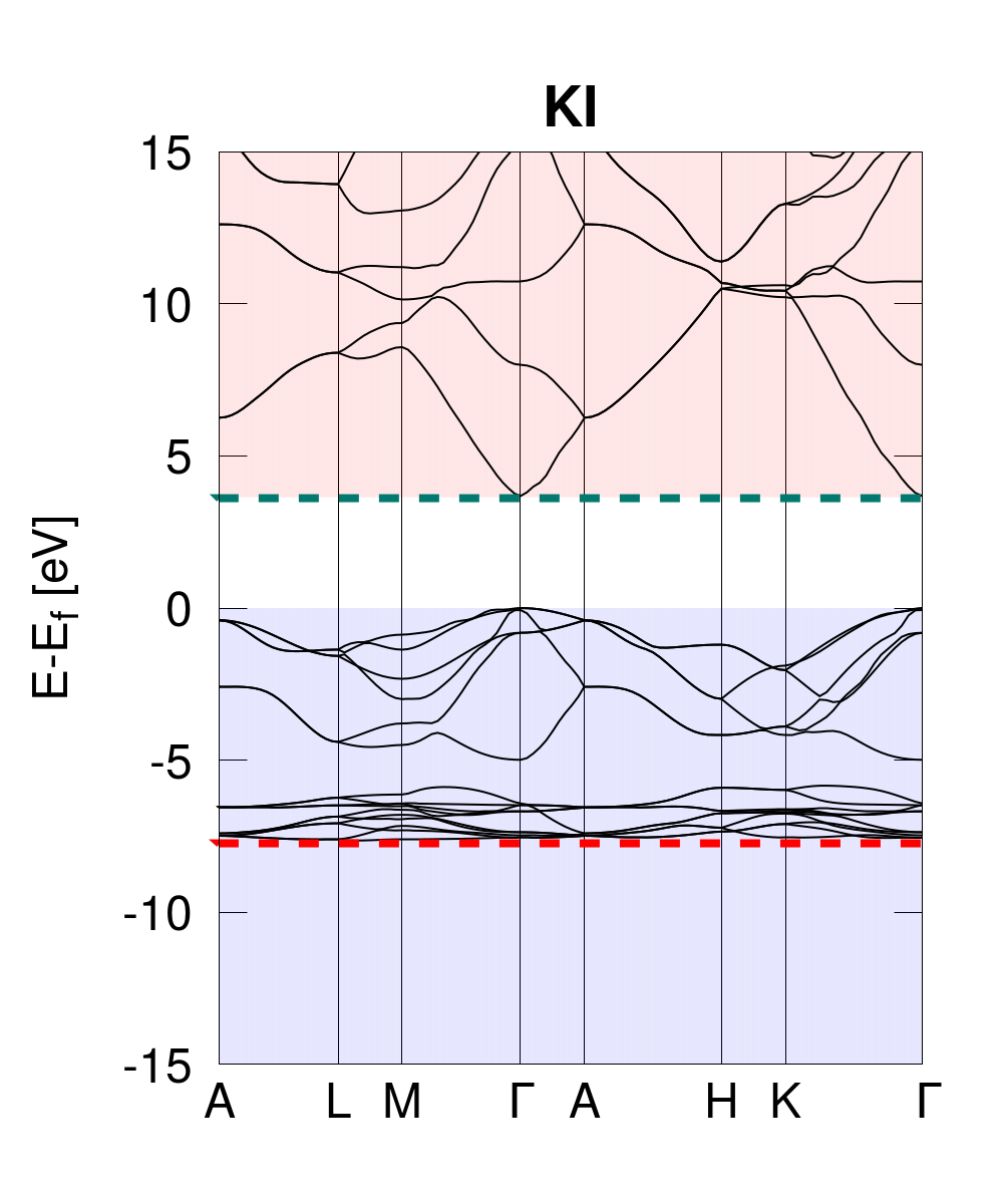
	LDA	HSE	GW0	scG$\tilde{\rm W}$	KI	Exp.
Egap(eV)	0.79	2.79	3.0	3.2	3.62	3.60(∗)
$\langle\varepsilon_{d}\rangle$(eV)	-5.1	-6.1	-6.4	-6.7	-6.9	-7.5/-8.0

Figure 5: Band structure of ZnO calculated at different level of theory: LDA (left panel), HSE (middle panel) and KI (right panel). Shaded areas highlight valence (light blue) and conduction (light red) manifolds. The experimental values for the band gap and for the energy position of Zn $d$-states are represented by the dashed green line and by the dashed red line, respectively. Table: Band gap and position of Zn $d$ states with respect to the top of the valence band at different level of theory compared to experimental and GW results from Ref. 112.^(∗) The zero-point-renormalization ¹²⁷ (-0.16 eV) has been subtracted to the experimental gap ¹¹² (3.44 eV) to have a meaningful comparison with the calculations.

It is worth mentioning here that for the KI calculation for ZnO we used projected Wannier functions as approximated variational orbitals. At variance with MLWFs, no minimization of the quadratic spread is performed in this case. The Wannier functions are uniquely defined by the projection onto atomic-like orbitals and, for the empty manifold, by the disentanglement procedure. We found that the minimization of the quadratic spread leads to a mixing of O $2p$ and Zn $3d$ states with deeper ones and this deteriorate the quality of the results (the band gap turns out to be overestimated and the $d$ states are pushed too low in energy). While the KS Hamiltonian depends only on the charge density and is therefore not affected by this unitary mixing, the orbital-density dependent part of the KI Hamiltonian is instead sensitive to the particular choice of the localized manifold; the unconstrained mixing of the valence Bloch states with very different energies is detrimental. The important question of which set of localized orbitals are the most suitable for the correction of the DFT Hamiltonian is not restricted to the KC functionals but is relevant, and has indeed been discussed, also in the context of the Perdew-Zunger self-interaction-correction scheme ⁷⁹, the generalized transition state method ^{70, 71}, the localized orbital scaling correction to approximate DFT ⁴² and the DFT+U method for predicting band gaps ¹²⁸. In principle the variational property of the KC functionals can be used to verify which set of Wannier functions — projected or maximally localized — is the most energetically favorable. This important point will be addressed in future work; here, we just highlight the evidence that in complex systems, where an undesired mixing between state with very different energies might be driven by the quadratic spread minimization, projected Wannier functions seem to provide a better choice for the localized manifold.

5 Summary and conclusions

We have developed, tested, and described a novel and efficient implementation of KC functional for periodic systems (but also readily applicable to finite ones) using Wannier functions as approximated variational orbitals and a linear response approach for the efficient evaluation of the screening parameters based on DFPT. Using the translational property of the Wannier functions , we have shown how to recast a problem whose natural dimension is that of a supercell, into a primitive cell problem plus a sampling of the primitive-cell Brillouin zone. All this leads to the decomposition of the problem into smaller and independent ones and thus to a sensible reduction of the computational cost and complexity. We have showcased its use to compute the band structure of few prototypical systems ranging from small gap semiconductors to a wide-gap insulator and demonstrated that the present implementation provides the same result as a straightforward supercell implementation, but at a greatly reduced computational cost, thus making the KC calculation more robust and user-friendly. The main results of Secs. (3.1.1) and (3.1.2) have been implemented as a post-processing of the PWSCF packages of the Quantum ESPRESSO  distribution ^{105, 104}, and of the Wannier90 code ¹⁰⁹, two open-source and widely used electronic structure tools. The KI implementation presented here is part of the official Quantum ESPRESSO  distribution. It is hosted at the Quantum ESPRESSO  gitlab repository under the name “KCW” and has been distributed with the official release $7.1$ of Quantum ESPRESSO . The data used to produce the results of this work are available at the Materials Cloud Archive. ¹²⁹

6 Acknowledgments

This work was supported by the Swiss National Science Foundation (SNSF) trough its National Centre of Competence in Research (NCCR) MARVEL and the grant No. 200021-179138.

References

- Marzari et al. 2021 Marzari, N.; Ferretti, A.; Wolverton, C. Electronic-structure methods for materials design. Nature Materials 2021, 20, 736–749, DOI: 10.1038/s41563-021-01013-3
- Hohenberg and Kohn 1964 Hohenberg, P.; Kohn, W. Inhomogeneous Electron Gas. Physical Review 1964, 136, B864–B871, DOI: 10.1103/PhysRev.136.B864
- Kohn and Sham 1965 Kohn, W.; Sham, L. J. Self-Consistent Equations Including Exchange and Correlation Effects. Physical Review 1965, 140, A1133–A1138, DOI: 10.1103/PhysRev.140.A1133
- Levy et al. 1984 Levy, M.; Perdew, J. P.; Sahni, V. Exact differential equation for the density and ionization energy of a many-particle system. Phys. Rev. A 1984, 30, 2745–2748, DOI: 10.1103/PhysRevA.30.2745
- Almbladh and von Barth 1985 Almbladh, C.-O.; von Barth, U. Exact results for the charge and spin densities, exchange-correlation potentials, and density-functional eigenvalues. Phys. Rev. B 1985, 31, 3231–3244, DOI: 10.1103/PhysRevB.31.3231
- Perdew and Levy 1997 Perdew, J. P.; Levy, M. Comment on “Significance of the highest occupied Kohn-Sham eigenvalue”. Phys. Rev. B 1997, 56, 16021–16028, DOI: 10.1103/PhysRevB.56.16021
- Chong et al. 2002 Chong, D. P.; Gritsenko, O. V.; Baerends, E. J. Interpretation of the Kohn–Sham orbital energies as approximate vertical ionization potentials. J. Chem. Phys. 2002, 116, 1760–1772, DOI: 10.1063/1.1430255
- Pederson et al. 1985 Pederson, M. R.; Heaton, R. A.; Lin, C. C. Density-functional theory with self-interaction correction: Application to the lithium moleculea). J. Chem. Phys. 1985, 82, DOI: 10.1063/1.448266
- Runge and Gross 1984 Runge, E.; Gross, E. K. U. Density-Functional Theory for Time-Dependent Systems. Physical Review Letters 1984, 52, 997–1000, DOI: 10.1103/PhysRevLett.52.997
- Onida et al. 2002 Onida, G.; Reining, L.; Rubio, A. Electronic excitations: density-functional versus many-body Green’s-function approaches. Reviews of Modern Physics 2002, 74, 601–659
- Hedin 1965 Hedin, L. New Method for Calculating the One-Particle Green’s Function with Application to the Electron-Gas Problem. Physical Review 1965, 139, A796–A823, DOI: 10.1103/PhysRev.139.A796
- Umari et al. 2009 Umari, P.; Stenuit, G.; Baroni, S. Optimal representation of the polarization propagator for large-scale GW calculations. Physical Review B 2009, 79, 201104, DOI: 10.1103/PhysRevB.79.201104
- Umari et al. 2010 Umari, P.; Stenuit, G.; Baroni, S. GW quasiparticle spectra from occupied states only. Physical Review B 2010, 81, 115104, DOI: 10.1103/PhysRevB.81.115104
- Giustino et al. 2010 Giustino, F.; Cohen, M. L.; Louie, S. G. GW method with the self-consistent Sternheimer equation. Physical Review B 2010, 81, 115105, DOI: 10.1103/PhysRevB.81.115105
- Neuhauser et al. 2014 Neuhauser, D.; Gao, Y.; Arntsen, C.; Karshenas, C.; Rabani, E.; Baer, R. Breaking the Theoretical Scaling Limit for Predicting Quasiparticle Energies: The Stochastic GW Approach. Physical Review Letters 2014, 113, 076402, DOI: 10.1103/PhysRevLett.113.076402
- Govoni and Galli 2015 Govoni, M.; Galli, G. Large Scale GW Calculations. Journal of Chemical Theory and Computation 2015, 11, 2680–2696, DOI: 10.1021/ct500958p
- Wilhelm et al. 2018 Wilhelm, J.; Golze, D.; Talirz, L.; Hutter, J.; Pignedoli, C. A. Toward GW Calculations on Thousands of Atoms. The Journal of Physical Chemistry Letters 2018, 9, 306–312, DOI: 10.1021/acs.jpclett.7b02740
- Vlček et al. 2018 Vlček, V.; Li, W.; Baer, R.; Rabani, E.; Neuhauser, D. Swift GW beyond 10,000 electrons using sparse stochastic compression. Physical Review B 2018, 98, 075107, DOI: 10.1103/PhysRevB.98.075107
- Umari 2022 Umari, P. A Fully Linear Response G0W0 Method That Scales Linearly up to Tens of Thousands of Cores. The Journal of Physical Chemistry A 2022, 126, 3384–3391, DOI: 10.1021/acs.jpca.2c01328
- Becke 1993 Becke, A. D. A new mixing of Hartree–Fock and local density-functional theories. The Journal of Chemical Physics 1993, 98, 1372–1377, DOI: 10.1063/1.464304
- Dabo et al. 2009 Dabo, I.; Cococcioni, M.; Marzari, N. Non-Koopmans Corrections in Density-functional Theory: Self-interaction Revisited. arXiv:0901.2637 [cond-mat] 2009, arXiv: 0901.2637
- Dabo et al. 2010 Dabo, I.; Ferretti, A.; Poilvert, N.; Li, Y.; Marzari, N.; Cococcioni, M. Koopmans’ condition for density-functional theory. Physical Review B 2010, 82, 115121, DOI: 10.1103/PhysRevB.82.115121
- Dabo et al. 2014 Dabo, I.; Ferretti, A.; Marzari, N. First Principles Approaches to Spectroscopic Properties of Complex Materials; Topics in Current Chemistry; Springer, Berlin, Heidelberg, 2014; pp 193–233, DOI: 10.1007/128_2013_504
- Borghi et al. 2014 Borghi, G.; Ferretti, A.; Nguyen, N. L.; Dabo, I.; Marzari, N. Koopmans-compliant functionals and their performance against reference molecular data. Physical Review B 2014, 90, 075135, DOI: 10.1103/PhysRevB.90.075135
- Borghi et al. 2015 Borghi, G.; Park, C.-H.; Nguyen, N. L.; Ferretti, A.; Marzari, N. Variational minimization of orbital-density-dependent functionals. Physical Review B 2015, 91, 155112, DOI: 10.1103/PhysRevB.91.155112
- Nguyen et al. 2018 Nguyen, N. L.; Colonna, N.; Ferretti, A.; Marzari, N. Koopmans-Compliant Spectral Functionals for Extended Systems. Physical Review X 2018, 8, 021051, DOI: 10.1103/PhysRevX.8.021051
- Ferretti et al. 2014 Ferretti, A.; Dabo, I.; Cococcioni, M.; Marzari, N. Bridging density-functional and many-body perturbation theory: Orbital-density dependence in electronic-structure functionals. Physical Review B 2014, 89, 195134, DOI: 10.1103/PhysRevB.89.195134
- Colonna et al. 2019 Colonna, N.; Nguyen, N. L.; Ferretti, A.; Marzari, N. Koopmans-Compliant Functionals and Potentials and Their Application to the GW100 Test Set. Journal of Chemical Theory and Computation 2019, 15, 1905–1914, DOI: 10.1021/acs.jctc.8b00976
- Perdew et al. 1982 Perdew, J. P.; Parr, R. G.; Levy, M.; Balduz, J. L. Density-Functional Theory for Fractional Particle Number: Derivative Discontinuities of the Energy. Physical Review Letters 1982, 49, 1691–1694, DOI: 10.1103/PhysRevLett.49.1691
- Cococcioni and de Gironcoli 2005 Cococcioni, M.; de Gironcoli, S. Linear response approach to the calculation of the effective interaction parameters in the LDA+U method. Phys. Rev. B 2005, 71, 035105, DOI: 10.1103/PhysRevB.71.035105
- Kulik et al. 2006 Kulik, H. J.; Cococcioni, M.; Scherlis, D. A.; Marzari, N. Density Functional Theory in Transition-Metal Chemistry: A Self-Consistent Hubbard U Approach. Phys. Rev. Lett. 2006, 97, 103001, DOI: 10.1103/PhysRevLett.97.103001
- Mori-Sánchez et al. 2006 Mori-Sánchez, P.; Cohen, A. J.; Yang, W. Many-electron self-interaction error in approximate density functionals. J. Chem. Phys. 2006, 125, 201102, DOI: 10.1063/1.2403848
- Cohen et al. 2008 Cohen, A. J.; Mori-Sánchez, P.; Yang, W. Insights into Current Limitations of Density Functional Theory. Science 2008, 321, 792–794, DOI: 10.1126/science.1158722
- Mori-Sánchez et al. 2008 Mori-Sánchez, P.; Cohen, A. J.; Yang, W. Localization and Delocalization Errors in Density Functional Theory and Implications for Band-Gap Prediction. Phys. Rev. Lett. 2008, 100, 146401, DOI: 10.1103/PhysRevLett.100.146401
- Perdew and Zunger 1981 Perdew, J. P.; Zunger, A. Self-interaction correction to density-functional approximations for many-electron systems. Phys. Rev. B 1981, 23, 5048–5079, DOI: 10.1103/PhysRevB.23.5048
- Zheng et al. 2011 Zheng, X.; Cohen, A. J.; Mori-Sánchez, P.; Hu, X.; Yang, W. Improving Band Gap Prediction in Density Functional Theory from Molecules to Solids. Phys. Rev. Lett. 2011, 107, 026403, DOI: 10.1103/PhysRevLett.107.026403
- Zheng et al. 2013 Zheng, X.; Zhou, T.; Yang, W. A nonempirical scaling correction approach for density functional methods involving substantial amount of Hartree–Fock exchange. The Journal of Chemical Physics 2013, 138, 174105, DOI: 10.1063/1.4801922
- Kraisler and Kronik 2013 Kraisler, E.; Kronik, L. Piecewise Linearity of Approximate Density Functionals Revisited: Implications for Frontier Orbital Energies. Phys. Rev. Lett. 2013, 110, 126403, DOI: 10.1103/PhysRevLett.110.126403
- Kraisler and Kronik 2014 Kraisler, E.; Kronik, L. Fundamental gaps with approximate density functionals: The derivative discontinuity revealed from ensemble considerations. The Journal of Chemical Physics 2014, 140, 18A540, DOI: 10.1063/1.4871462
- Li et al. 2015 Li, C.; Zheng, X.; Cohen, A. J.; Mori-Sánchez, P.; Yang, W. Local Scaling Correction for Reducing Delocalization Error in Density Functional Approximations. Phys. Rev. Lett. 2015, 114, 053001, DOI: 10.1103/PhysRevLett.114.053001
- Görling 2015 Görling, A. Exchange-correlation potentials with proper discontinuities for physically meaningful Kohn-Sham eigenvalues and band structures. Phys. Rev. B 2015, 91, 245120, DOI: 10.1103/PhysRevB.91.245120
- Li et al. 2018 Li, C.; Zheng, X.; Su, N. Q.; Yang, W. Localized orbital scaling correction for systematic elimination of delocalization error in density functional approximations. National Science Review 2018, 5, 203–215, DOI: 10.1093/nsr/nwx111
- Mei et al. 2021 Mei, Y.; Chen, Z.; Yang, W. The Exact Second Order Corrections and Accurate Quasiparticle Energy Calculations in Density Functional Theory. arXiv:2106.10358 [physics, physics:quant-ph] 2021, arXiv: 2106.10358
- Stein et al. 2010 Stein, T.; Eisenberg, H.; Kronik, L.; Baer, R. Fundamental Gaps in Finite Systems from Eigenvalues of a Generalized Kohn-Sham Method. Phys. Rev. Lett. 2010, 105, 266802, DOI: 10.1103/PhysRevLett.105.266802
- Kronik et al. 2012 Kronik, L.; Stein, T.; Refaely-Abramson, S.; Baer, R. Excitation Gaps of Finite-Sized Systems from Optimally Tuned Range-Separated Hybrid Functionals. J. Chem. Theory Comput. 2012, 8, 1515–1531, DOI: 10.1021/ct2009363
- Refaely-Abramson et al. 2012 Refaely-Abramson, S.; Sharifzadeh, S.; Govind, N.; Autschbach, J.; Neaton, J. B.; Baer, R.; Kronik, L. Quasiparticle Spectra from a Nonempirical Optimally Tuned Range-Separated Hybrid Density Functional. Phys. Rev. Lett. 2012, 109, 226405
- Shimazaki and Asai 2008 Shimazaki, T.; Asai, Y. Band structure calculations based on screened Fock exchange method. Chemical Physics Letters 2008, 466, 91 – 94, DOI: https://doi.org/10.1016/j.cplett.2008.10.012
- Marques et al. 2011 Marques, M. A. L.; Vidal, J.; Oliveira, M. J. T.; Reining, L.; Botti, S. Density-based mixing parameter for hybrid functionals. Phys. Rev. B 2011, 83, 035119, DOI: 10.1103/PhysRevB.83.035119
- Skone et al. 2014 Skone, J. H.; Govoni, M.; Galli, G. Self-consistent hybrid functional for condensed systems. Phys. Rev. B 2014, 89, 195112, DOI: 10.1103/PhysRevB.89.195112
- Brawand et al. 2016 Brawand, N. P.; Vörös, M.; Govoni, M.; Galli, G. Generalization of Dielectric-Dependent Hybrid Functionals to Finite Systems. Phys. Rev. X 2016, 6, 041002, DOI: 10.1103/PhysRevX.6.041002
- Dabo et al. 2012 Dabo, I.; Ferretti, A.; Park, C.-H.; Poilvert, N.; Li, Y.; Cococcioni, M.; Marzari, N. Donor and acceptor levels of organic photovoltaic compounds from first principles. Physical Chemistry Chemical Physics 2012, 15, 685–695, DOI: 10.1039/C2CP43491A
- Nguyen et al. 2015 Nguyen, N. L.; Borghi, G.; Ferretti, A.; Dabo, I.; Marzari, N. First-Principles Photoemission Spectroscopy and Orbital Tomography in Molecules from Koopmans-Compliant Functionals. Physical Review Letters 2015, 114, 166405, DOI: 10.1103/PhysRevLett.114.166405
- Nguyen et al. 2016 Nguyen, N. L.; Borghi, G.; Ferretti, A.; Marzari, N. First-Principles Photoemission Spectroscopy of DNA and RNA Nucleobases from Koopmans-Compliant Functionals. Journal of Chemical Theory and Computation 2016, 12, 3948–3958, DOI: 10.1021/acs.jctc.6b00145
- Elliott et al. 2019 Elliott, J. D.; Colonna, N.; Marsili, M.; Marzari, N.; Umari, P. Koopmans Meets Bethe–Salpeter: Excitonic Optical Spectra without GW. Journal of Chemical Theory and Computation 2019, DOI: 10.1021/acs.jctc.8b01271
- de Almeida et al. 2021 de Almeida, J. M.; Nguyen, N. L.; Colonna, N.; Chen, W.; Rodrigues Miranda, C.; Pasquarello, A.; Marzari, N. Electronic Structure of Water from Koopmans-Compliant Functionals. Journal of Chemical Theory and Computation 2021, 17, 3923–3930, DOI: 10.1021/acs.jctc.1c00063
- Gatti et al. 2007 Gatti, M.; Olevano, V.; Reining, L.; Tokatly, I. V. Transforming Nonlocality into a Frequency Dependence: A Shortcut to Spectroscopy. Physical Review Letters 2007, 99, 057401, DOI: 10.1103/PhysRevLett.99.057401
- Vanzini et al. 2017 Vanzini, M.; Reining, L.; Gatti, M. Dynamical local connector approximation for electron addition and removal spectra. arXiv:1708.02450 [cond-mat] 2017, arXiv: 1708.02450
- Vanzini et al. 2018 Vanzini, M.; Reining, L.; Gatti, M. Spectroscopy of the Hubbard dimer: the spectral potential. The European Physical Journal B 2018, 91, 192, DOI: 10.1140/epjb/e2018-90277-3
- Zhang et al. 2015 Zhang, D.; Zheng, X.; Li, C.; Yang, W. Orbital relaxation effects on Kohn–Sham frontier orbital energies in density functional theory. The Journal of Chemical Physics 2015, 142, 154113, DOI: 10.1063/1.4918347
- Colonna et al. 2018 Colonna, N.; Nguyen, N. L.; Ferretti, A.; Marzari, N. Screening in Orbital-Density-Dependent Functionals. Journal of Chemical Theory and Computation 2018, 14, 2549–2557, DOI: 10.1021/acs.jctc.7b01116
- De Gennaro et al. 2021 De Gennaro, R.; Colonna, N.; Linscott, E.; Marzari, N. Bloch’s theorem in orbital-density-dependent functionals: band structures from Koopmans spectral functionals. arXiv:2111.09550 [cond-mat, physics:physics] 2021,
- Boys 1960 Boys, S. F. Construction of Some Molecular Orbitals to Be Approximately Invariant for Changes from One Molecule to Another. Rev. Mod. Phys. 1960, 32, 296–299, DOI: 10.1103/RevModPhys.32.296
- Foster and Boys 1960 Foster, J. M.; Boys, S. F. Canonical Configurational Interaction Procedure. Rev. Mod. Phys. 1960, 32, 300–302, DOI: 10.1103/RevModPhys.32.300
- Marzari and Vanderbilt 1997 Marzari, N.; Vanderbilt, D. Maximally localized generalized Wannier functions for composite energy bands. Physical Review B 1997, 56, 12847–12865, DOI: 10.1103/PhysRevB.56.12847
- Marzari et al. 2012 Marzari, N.; Mostofi, A. A.; Yates, J. R.; Souza, I.; Vanderbilt, D. Maximally localized Wannier functions: Theory and applications. Rev. Mod. Phys. 2012, 84, 1419–1475, DOI: 10.1103/RevModPhys.84.1419
- Miceli et al. 2018 Miceli, G.; Chen, W.; Reshetnyak, I.; Pasquarello, A. Nonempirical hybrid functionals for band gaps and polaronic distortions in solids. Physical Review B 2018, 97, 121112, DOI: 10.1103/PhysRevB.97.121112
- Bischoff et al. 2019 Bischoff, T.; Reshetnyak, I.; Pasquarello, A. Adjustable potential probes for band-gap predictions of extended systems through nonempirical hybrid functionals. Physical Review B 2019, 99, 201114, DOI: 10.1103/PhysRevB.99.201114
- Bischoff et al. 2019 Bischoff, T.; Wiktor, J.; Chen, W.; Pasquarello, A. Nonempirical hybrid functionals for band gaps of inorganic metal-halide perovskites. Physical Review Materials 2019, 3, 123802, DOI: 10.1103/PhysRevMaterials.3.123802
- Heaton et al. 1983 Heaton, R. A.; Harrison, J. G.; Lin, C. C. Self-interaction correction for density-functional theory of electronic energy bands of solids. Physical Review B 1983, 28, 5992–6007, DOI: 10.1103/PhysRevB.28.5992
- Anisimov and Kozhevnikov 2005 Anisimov, V. I.; Kozhevnikov, A. V. Transition state method and Wannier functions. Physical Review B 2005, 72, 075125, DOI: 10.1103/PhysRevB.72.075125
- Ma and Wang 2016 Ma, J.; Wang, L.-W. Using Wannier functions to improve solid band gap predictions in density functional theory. Scientific Reports 2016, 6, 24924, DOI: 10.1038/srep24924
- Weng et al. 2018 Weng, M.; Li, S.; Zheng, J.; Pan, F.; Wang, L.-W. Wannier Koopmans Method Calculations of 2D Material Band Gaps. The Journal of Physical Chemistry Letters 2018, 9, 281–285, DOI: 10.1021/acs.jpclett.7b03041
- Weng et al. 2020 Weng, M.; Pan, F.; Wang, L.-W. Wannier–Koopmans method calculations for transition metal oxide band gaps. npj Computational Materials 2020, 6, 1–8, DOI: 10.1038/s41524-020-0302-0
- Wing et al. 2021 Wing, D.; Ohad, G.; Haber, J. B.; Filip, M. R.; Gant, S. E.; Neaton, J. B.; Kronik, L. Band gaps of crystalline solids from Wannier-localization–based optimal tuning of a screened range-separated hybrid functional. Proceedings of the National Academy of Sciences 2021, 118, DOI: 10.1073/pnas.2104556118
- Shinde et al. 2020 Shinde, R.; Yamijala, S. S. R. K. C.; Wong, B. M. Improved Band Gaps and Structural Properties from Wannier-Fermi-Löwdin Self-Interaction Corrections for Periodic Systems. Journal of Physics: Condensed Matter 2020, 33, 115501, DOI: 10.1088/1361-648X/abc407
- Pederson et al. 1984 Pederson, M. R.; Heaton, R. A.; Lin, C. C. Local-density Hartree–Fock theory of electronic states of molecules with self-interaction correction. J. Chem. Phys. 1984, 80, 1972–1975, DOI: 10.1063/1.446959
- Lehtola and Jónsson 2014 Lehtola, S.; Jónsson, H. Variational, Self-Consistent Implementation of the Perdew–Zunger Self-Interaction Correction with Complex Optimal Orbitals. J. Chem. Theory Comput. 2014, 10, 5324–5337, DOI: 10.1021/ct500637x
- Vydrov et al. 2007 Vydrov, O. A.; Scuseria, G. E.; Perdew, J. P. Tests of functionals for systems with fractional electron number. J. Chem. Phys. 2007, 126, 154109, DOI: 10.1063/1.2723119
- Stengel and Spaldin 2008 Stengel, M.; Spaldin, N. A. Self-interaction correction with Wannier functions. Phys. Rev. B 2008, 77, 155106, DOI: 10.1103/PhysRevB.77.155106
- Hofmann et al. 2012 Hofmann, D.; Klüpfel, S.; Klüpfel, P.; Kümmel, S. Using complex degrees of freedom in the Kohn-Sham self-interaction correction. Phys. Rev. A 2012, 85, 062514, DOI: 10.1103/PhysRevA.85.062514
- Marzari et al. 1997 Marzari, N.; Vanderbilt, D.; Payne, M. C. Ensemble Density-Functional Theory for Ab Initio Molecular Dynamics of Metals and Finite-Temperature Insulators. Phys. Rev. Lett. 1997, 79, 1337–1340, DOI: 10.1103/PhysRevLett.79.1337
- Wannier 1937 Wannier, G. H. The Structure of Electronic Excitation Levels in Insulating Crystals. Physical Review 1937, 52, 191–197, DOI: 10.1103/PhysRev.52.191
- Salzner and Baer 2009 Salzner, U.; Baer, R. Koopmans’ springs to life. J. Chem. Phys. 2009, 131, 231101, DOI: 10.1063/1.3269030
- Stein et al. 2012 Stein, T.; Autschbach, J.; Govind, N.; Kronik, L.; Baer, R. Curvature and Frontier Orbital Energies in Density Functional Theory. J. Phys. Chem. Lett. 2012, 3, 3740–3744, DOI: 10.1021/jz3015937
- Weng et al. 2017 Weng, M.; Li, S.; Ma, J.; Zheng, J.; Pan, F.; Wang, L.-W. Wannier Koopman method calculations of the band gaps of alkali halides. Applied Physics Letters 2017, 111, 054101, DOI: 10.1063/1.4996743
- Li et al. 2018 Li, S.; Weng, M.; Jie, J.; Zheng, J.; Pan, F.; Wang, L.-W. Wannier-Koopmans method calculations of organic molecule crystal band gaps. EPL (Europhysics Letters) 2018, 123, 37002, DOI: 10.1209/0295-5075/123/37002
- Baroni et al. 2001 Baroni, S.; de Gironcoli, S.; Dal Corso, A.; Giannozzi, P. Phonons and related crystal properties from density-functional perturbation theory. Rev. Mod. Phys. 2001, 73, 515–562, DOI: 10.1103/RevModPhys.73.515
- Timrov et al. 2018 Timrov, I.; Marzari, N.; Cococcioni, M. Hubbard parameters from density-functional perturbation theory. Physical Review B 2018, 98, 085127, DOI: 10.1103/PhysRevB.98.085127
- Timrov et al. 2021 Timrov, I.; Marzari, N.; Cococcioni, M. Self-consistent Hubbard parameters from density-functional perturbation theory in the ultrasoft and projector-augmented wave formulations. Physical Review B 2021, 103, 045141, DOI: 10.1103/PhysRevB.103.045141
- Slater and Koster 1954 Slater, J. C.; Koster, G. F. Simplified LCAO Method for the Periodic Potential Problem. Physical Review 1954, 94, 1498–1524, DOI: 10.1103/PhysRev.94.1498
- Souza et al. 2001 Souza, I.; Marzari, N.; Vanderbilt, D. Maximally localized Wannier functions for entangled energy bands. Physical Review B 2001, 65, 035109, DOI: 10.1103/PhysRevB.65.035109
- Makov and Payne 1995 Makov, G.; Payne, M. C. Periodic boundary conditions in \textit{ab initio} calculations. Phys. Rev. B 1995, 51, 4014–4022, DOI: 10.1103/PhysRevB.51.4014
- Ismail-Beigi 2006 Ismail-Beigi, S. Truncation of periodic image interactions for confined systems. Physical Review B 2006, 73, 233103, DOI: 10.1103/PhysRevB.73.233103
- Rozzi et al. 2006 Rozzi, C. A.; Varsano, D.; Marini, A.; Gross, E. K. U.; Rubio, A. Exact Coulomb cutoff technique for supercell calculations. Physical Review B 2006, 73, 205119, DOI: 10.1103/PhysRevB.73.205119
- Martyna and Tuckerman 1999 Martyna, G. J.; Tuckerman, M. E. A reciprocal space based method for treating long range interactions in ab initio and force-field-based calculations in clusters. J. Chem. Phys. 1999, 110, 2810–2821, DOI: 10.1063/1.477923
- Dabo et al. 2008 Dabo, I.; Kozinsky, B.; Singh-Miller, N. E.; Marzari, N. Electrostatics in periodic boundary conditions and real-space corrections. Physical Review B 2008, 77, 115139, DOI: 10.1103/PhysRevB.77.115139
- Gygi and Baldereschi 1989 Gygi, F.; Baldereschi, A. Quasiparticle energies in semiconductors: Self-energy correction to the local-density approximation. Phys. Rev. Lett. 1989, 62, 2160–2163, DOI: 10.1103/PhysRevLett.62.2160
- Nguyen and de Gironcoli 2009 Nguyen, H.-V.; de Gironcoli, S. Efficient calculation of exact exchange and RPA correlation energies in the adiabatic-connection fluctuation-dissipation theory. Phys. Rev. B 2009, 79, 205114, DOI: 10.1103/PhysRevB.79.205114
- Fischerauer 1997 Fischerauer, G. Comments on real-space Green’s function of an isolated point-charge in an unbounded anisotropic medium. IEEE Transactions on Ultrasonics, Ferroelectrics, and Frequency Control 1997, 44, 1179–1180, DOI: 10.1109/58.656617
- Rurali and Cartoixà 2009 Rurali, R.; Cartoixà, X. Theory of Defects in One-Dimensional Systems: Application to Al-Catalyzed Si Nanowires. Nano Letters 2009, 9, 975–979, DOI: 10.1021/nl802847p
- Murphy and Hine 2013 Murphy, S. T.; Hine, N. D. M. Anisotropic charge screening and supercell size convergence of defect formation energies. Physical Review B 2013, 87, 094111, DOI: 10.1103/PhysRevB.87.094111
- Heyd et al. 2003 Heyd, J.; Scuseria, G. E.; Ernzerhof, M. Hybrid functionals based on a screened Coulomb potential. The Journal of Chemical Physics 2003, 118, 8207–8215, DOI: 10.1063/1.1564060
- Heyd et al. 2006 Heyd, J.; Scuseria, G. E.; Ernzerhof, M. Erratum: “Hybrid functionals based on a screened Coulomb potential” [J. Chem. Phys.118, 8207 (2003)]. The Journal of Chemical Physics 2006, 124, 219906, DOI: 10.1063/1.2204597
- Giannozzi et al. 2009 Giannozzi, P. et al. QUANTUM ESPRESSO: a modular and open-source software project for quantum simulations of materials. Journal of Physics: Condensed Matter 2009, 21, 395502, DOI: 10.1088/0953-8984/21/39/395502
- Giannozzi et al. 2017 Giannozzi, P. et al. Advanced capabilities for materials modelling with Q uantum ESPRESSO. Journal of Physics: Condensed Matter 2017, 29, 465901, DOI: 10.1088/1361-648X/aa8f79
- Hamann 2013 Hamann, D. R. Optimized norm-conserving Vanderbilt pseudopotentials. Physical Review B 2013, 88, 085117, DOI: 10.1103/PhysRevB.88.085117
- Hamann 2017 Hamann, D. R. Erratum: Optimized norm-conserving Vanderbilt pseudopotentials [Phys. Rev. B 88, 085117 (2013)]. Phys. Rev. B 2017, 95, 239906
- van Setten et al. 2018 van Setten, M. J.; Giantomassi, M.; Bousquet, E.; Verstraete, M. J.; Hamann, D. R.; Gonze, X.; Rignanese, G. M. The PseudoDojo: Training and grading a 85 element optimized norm-conserving pseudopotential table. Computer Physics Communications 2018, 226, 39–54, DOI: 10.1016/j.cpc.2018.01.012
- Pizzi et al. 2020 Pizzi, G. et al. Wannier90 as a community code: new features and applications. Journal of Physics: Condensed Matter 2020, 32, 165902, DOI: 10.1088/1361-648x/ab51ff
- Shevchik et al. 1974 Shevchik, N. J.; Tejeda, J.; Cardona, M. Densities of valence states of amorphous and crystalline III-V and II-VI semiconductors. Physical Review B 1974, 9, 2627–2648, DOI: 10.1103/PhysRevB.9.2627
- Madelung 2004 Madelung, O. Semiconductors: Data Handbook; Springer-Verlag, 2004; DOI: 10.1007/978-3-642-18865-7
- Shishkin et al. 2007 Shishkin, M.; Marsman, M.; Kresse, G. Accurate Quasiparticle Spectra from Self-Consistent GW Calculations with Vertex Corrections. Phys. Rev. Lett. 2007, 99, 246403, DOI: 10.1103/PhysRevLett.99.246403
- Brawand et al. 2017 Brawand, N. P.; Govoni, M.; Vörös, M.; Galli, G. Performance and Self-Consistency of the Generalized Dielectric Dependent Hybrid Functional. Journal of Chemical Theory and Computation 2017, DOI: 10.1021/acs.jctc.7b00368
- Shishkin and Kresse 2007 Shishkin, M.; Kresse, G. Self-consistent GW calculations for semiconductors and insulators. Physical Review B 2007, 75, 235102, DOI: 10.1103/PhysRevB.75.235102
- Wang et al. 2003 Wang, N.-P.; Rohlfing, M.; Krüger, P.; Pollmann, J. Quasiparticle band structure and optical spectrum of LiF(001). Physical Review B 2003, 67, 115111, DOI: 10.1103/PhysRevB.67.115111
- Piacentini et al. 1976 Piacentini, M.; Lynch, D. W.; Olson, C. G. Thermoreflectance of LiF between 12 and 30 eV. Physical Review B 1976, 13, 5530–5543, DOI: 10.1103/PhysRevB.13.5530
- Johansson and Hagström 1976 Johansson, L. I.; Hagström, S. B. M. Core Level and Band Structure Energies of the Alkali Halides LiF, LiCl and LiBr Studied by ESCA. Physica Scripta 1976, 14, 55–59, DOI: 10.1088/0031-8949/14/1-2/011
- Nery et al. 2018 Nery, J. P.; Allen, P. B.; Antonius, G.; Reining, L.; Miglio, A.; Gonze, X. Quasiparticles and phonon satellites in spectral functions of semiconductors and insulators: Cumulants applied to the full first-principles theory and the Fr\”ohlich polaron. Physical Review B 2018, 97, 115145, DOI: 10.1103/PhysRevB.97.115145
- Look and Claflin 2004 Look, D. C.; Claflin, B. P-type doping and devices based on ZnO. physica status solidi (b) 2004, 241, 624–630, DOI: https://doi.org/10.1002/pssb.200304271
- Look et al. 2004 Look, D. C.; Claflin, B.; Alivov, Y. I.; Park, S. J. The future of ZnO light emitters. physica status solidi (a) 2004, 201, 2203–2212, DOI: https://doi.org/10.1002/pssa.200404803
- Özgür et al. 2005 Özgür, Ü.; Alivov, Y. I.; Liu, C.; Teke, A.; Reshchikov, M. A.; Doğan, S.; Avrutin, V.; Cho, S.-J.; Morkoç, H. A comprehensive review of ZnO materials and devices. Journal of Applied Physics 2005, 98, 041301, DOI: 10.1063/1.1992666
- Look 2006 Look, D. C. Progress in ZnO materials and devices. Journal of Electronic Materials 2006, 35, 1299–1305, DOI: 10.1007/s11664-006-0258-y
- Shih et al. 2010 Shih, B.-C.; Xue, Y.; Zhang, P.; Cohen, M. L.; Louie, S. G. Quasiparticle Band Gap of ZnO: High Accuracy from the Conventional GW Approach. Physical Review Letters 2010, 105, 146401, DOI: 10.1103/PhysRevLett.105.146401
- Samsonidze et al. 2014 Samsonidze, G.; Par k, C.-H.; Kozinsky, B. Insights and challenges of applying theGWmethod to transition metal oxides. Journal of Physics: Condensed Matter 2014, 26, 475501, DOI: 10.1088/0953-8984/26/47/475501
- Wei and Zunger 1988 Wei, S.-H.; Zunger, A. Role of metal d states in II-VI semiconductors. Physical Review B 1988, 37, 8958–8981, DOI: 10.1103/PhysRevB.37.8958
- Lim et al. 2012 Lim, L. Y.; Lany, S.; Chang, Y. J.; Rotenberg, E.; Zunger, A.; Toney, M. F. Angle-resolved photoemission and quasiparticle calculation of ZnO: The need for band shift in oxide semiconductors. Physical Review B 2012, 86, 235113, DOI: 10.1103/PhysRevB.86.235113
- Cardona and Thewalt 2005 Cardona, M.; Thewalt, M. L. W. Isotope effects on the optical spectra of semiconductors. Reviews of Modern Physics 2005, 77, 1173–1224, DOI: 10.1103/RevModPhys.77.1173
- Kirchner-Hall et al. 2021 Kirchner-Hall, N. E.; Zhao, W.; Xiong, Y.; Timrov, I.; Dabo, I. Extensive Benchmarking of DFT+U Calculations for Predicting Band Gaps. Applied Sciences 2021, 11, 2395, DOI: 10.3390/app11052395
- Colonna et al. 2021 Colonna, N.; De Gennaro, R.; Linscott, E.; Marzari, N. Koopmans spectral functionals: an open-source periodic-boundary implementation. Materials Cloud Archive 2021.85 2021, DOI: 10.24435/materialscloud:b5-8r