Extended Kalman filter based observer design for semilinear infinite-dimensional systems

Abstract

In many physical applications, the system’s state varies with spatial variables as well as time. The state of such systems is modelled by partial differential equations and evolves on an infinite-dimensional space. Systems modelled by delay-differential equations are also infinite-dimensional systems. The full state of these systems cannot be measured. Observer design is an important tool for estimating the state from available measurements. For linear systems, both finite- and infinite-dimensional, the Kalman filter provides an estimate with minimum-variance on the error, if certain assumptions on the noise are satisfied. The extended Kalman filter (EKF) is one type of extension to nonlinear finite-dimensional systems. In this paper we provide an extension of the EKF to semilinear infinite-dimensional systems. Under mild assumptions we prove the well-posedness of equations defining the EKF. Local exponential stability of the error dynamics is shown. Only detectability is assumed, not observability, so this result is new even for finite-dimensional systems. The results are illustrated with implementation of finite-dimensional approximations of the infinite-dimensional EKF on an example.

I Introduction

In many physical applications, the system’s state varies with spatial variables as well as time. The state of such systems is modelled by partial differential equations and evolves on an infinite-dimensional space, and so they are an important class of infinite-dimensional systems. Systems modelled by delay-differential equations are also infinite-dimensional systems. The full state of these systems cannot be measured. As for finite-dimensional systems, a system, referred to as an observer or estimator, can be designed to estimate the state using the mathematical model and the measurements provided by sensors.

For linear systems, the Kalman filter (KF) minimizes the variance of the error under certain assumptions on the disturbances. The observer can be calculated through solution of a Riccati equation. The Kalman filter is widely used and was extended to infinite-dimensional linear systems in the 1970’s; see the review papers [1] and [2]. This theory was recently extended to time-varying infinite-dimensional systems [3]. For linear infinite-dimensional systems, there are a number of other different approaches to observer design in addition to the Kalman filter, including backstepping [4], sliding mode combined with backstepping [5]. Some other approaches can be found in [6, 7, 8, 9].

Due to its success in a wide range of applications, an extension of the KF to nonlinear systems, the extended Kalman filter (EKF), was developed for finite-dimensional systems. The EKF design is based on a linear approximation of the system around the estimated state. The linearized system is used to derive a Riccati equation and this is used to calculate the observer gain; e.g. [10, 11]. This method is widely used; see for example, [12, 13, 14, 15, 16, 17]. However, although this method may work well, it is well known that it may lead to divergent error estimates. Convergence of the estimation error for EKF depends on the size of the nonlinearity and the initial condition, see for instance, [18, 19].

Local asymptotic convergence of the estimation error under an observability assumption of the nonlinear system has been shown in [20, 21]. In [22], conditions for asymptotic convergence are imposed on the linearization residues. Under an uniform observability condition it is shown in [13, 14], that the estimation error is bounded in presence of disturbances. Local exponential convergence of the estimation error under uniform controllability and detectability conditions is shown in [23]. Local exponential convergence of the error is proven in [24] under certain assumptions that imply observability; similar results for discrete time are in [13]. In [25] better convergence was obtained by using the normal form of the governing ordinary differential equations. Local asymptotic convergence of the estimation error with an assumption of observability of the nonlinear system was subsequently shown in [20, 21].

Observers for nonlinear infinite-dimensional systems are often designed using a finite-dimensional approximation of the system. This enables the use of techniques for nonlinear finite-dimensional systems. Some examples are the robust fuzzy and also robust adaptive observers in [26] and [27]. In [28] the effect of approximation on observer performance for several different types of diffusion models and different observer designs was studied. The EKF has been used on finite-dimensional approximations of PDEs; for example a highway traffic model in [29] and state-of-charge estimation in lithium-ion batteries [30].

There are some studies for nonlinear infinite-dimensional systems where the observer is designed directly using the infinite-dimensional system equations. In [31], a second-order sliding mode observer is employed to provide stability with the assumption that the measurement is available everywhere. In [32], the observer dynamics are corrected by a linear output error injection term via an estimated spatially distributed measurement. Spatially-distributed linear output injection is also proposed in [33] for a one-dimensional nonlinear Burgers’ equation. Backstepping is used in [8] to design an observer for a lithium-ion battery model using the PDE model directly. An example of a general and abstract form of late lumping nonlinear observer design is introduced in [34] on reflexive Banach spaces, where a nonlinear feedback operator is added to a copy of the system’s dynamics. Other examples of observer design for specific nonlinear PDEs can be found in [35, 36, 37, 38]

In this paper, the EKF is formally shown to be well-posed for a class of semilinear infinite-dimensional systems with bounded observation. As for a finite-dimensional EKF, the observer dynamics are a copy of the original system’s dynamics with an injection gain defined by the solution of an Riccati equation. Since the Riccati equation is coupled with the observer equation, conventional results in the literature including [39] for existence of solutions to the Riccati equation cannot be directly used. This is due to the fact that for linear equations the Riccati equation does not depend on the state of the system. In our, nonlinear, case, such a dependence still remains after linearizing the system, making the analysis more involved. The proof of well-posedness was done in [40] for nonlinearities without time dependence, and briefly sketched in the conference paper [41]. A complete proof with a slightly different presentation and considering time-dependent nonlinearities is provided in this paper, and a more complex example is presented than in [41].

It is also shown that for sufficiently small initial error, and smooth nonlinearity, the error dynamics are exponentially stable. The approach for finite-dimensional systems cannot be used here because the analogue of the observability assumption would be uniformly exact observability, which is extremely restrictive for infinite-dimensional systems. Local exponential stability of the error dynamics is shown with much weaker assumptions of uniform stabilizability/detectabilty. Thus, these results are new even for finite-dimensional systems. The estimation error bounded in presence of disturbances. Although an EKF is generally implemented in discrete time, the analysis throughout is for a continuous time observer in order to remove the effects of time discretization from those of linearization.

For implementation, the infinite-dimensional EKF must be approximated using some method. The paper concludes with illustration of implementation of this approach for estimation of concentration in a magnetic drug delivery system.

Notation

Throughout the paper, calligraphic $\mathcal{H}$, with or without indices, will denote Hilbert spaces. Where the space considered is not clear from the context, the norm $\|\cdot\|$, as well as the scalar product $(\cdot,\cdot)$ will be equipped with an appropriate subscript, i.e. $\|\cdot\|_{\mathcal{H}}$ or $(\cdot,\cdot)_{\mathcal{H}}$; otherwise it is omitted. For an arbitrary, but henceforth fixed $t_{f}>0$ we work on the time interval $[0,t_{f}]$. For $0<p<\infty$ let $\mathbb{L}^{p}([0,t_{f}],\mathcal{H})$ and $\mathbb{W}^{1,p}([0,t_{f}],\mathcal{H})$ denote the spaces of functions ${f}:[0,t_{f}]\rightarrow\mathcal{H}$ such that

$$\int_{0}^{t_{f}}\|{f}(t)\|^{p}_{\mathcal{H}}\,ds<\infty\quad\text{and}\quad\int_{0}^{t}\|{f}(t)\|^{p}_{\mathcal{H}}+\|\frac{d}{dt}{f}(t)\|^{p}_{\mathcal{H}}\,ds<\infty$$

respectively. By $\mathcal{H}_{2}\hookrightarrow\mathcal{H}_{1}$ we denote a continuous and dense embedding and the trace space of $\mathbb{L}^{p}([0,t_{f}];\mathcal{H}_{2})\cap\mathbb{W}^{p}([0,t_{f}];\mathcal{H}_{1})$ is denoted by $\mathbb{H}_{p,1/p}.$ For integers $k\geq 0$ we denote by $\mathcal{C}^{k}([0,t_{f}],\mathcal{H})$ the space of functions $f:[0,t_{f}]:\rightarrow\mathcal{H}$ that are $k$ times continuously (with respect to the norm in $\mathcal{H}$) differentiable. Whenever $\mathcal{H}=\mathbb{R}$ we may omit the space and simply write $\mathbb{L}([0,t_{f}]),\mathbb{W}^{1,p}([0,t_{f}])$ and $\mathcal{C}^{k}([0,t_{f}])$ for the spaces above. For a linear operator ${A}:\mathcal{H}_{1}\rightarrow\mathcal{H}_{2}$ we write $\mathcal{D}({A})\subset\mathcal{H}_{1}$ for its domain and denote by

$$\|{A}\|=\sup_{{v}\in\mathcal{H}_{1}:\|{v}\|\leq 1}\|{A}{v}\|_{\mathcal{H}_{2}}$$

the usual operator norm. For nonlinear operators ${F}:\mathcal{H}_{1}\rightarrow\mathcal{H}_{2}$ we use brackets ${F}({v})$ whenever we write ${F}$ acting on ${v}\in\mathcal{H}_{1}$. Lastly, by $\mathcal{L}(\mathcal{H}_{1},\mathcal{H}_{2})$ we mean the space of linear and bounded operators mapping from $\mathcal{H}_{1}$ to $\mathcal{H}_{2}$, where we use the convention $\mathcal{L}(\mathcal{H})=\mathcal{L}(\mathcal{H},\mathcal{H}).$

II Preliminaries and statement of observer design problem

Let ${A}:\mathcal{D}({A})\rightarrow\mathcal{H}$ be a linear operator that generates a $C_{0}$-semigroup ${T}(t)$ on $\mathcal{H}$ and ${F}:\mathcal{H}\times[0,t_{f}]\rightarrow\mathcal{H}$ be strongly continuous in time and nonlinear on $\mathcal{H}$ satisfying ${F}(0,t)=0$ for every $t$.

We consider the semilinear evolution system

$$\frac{\partial{z}(t)}{\partial t} ={A}{z}(t)+{F}({z}(t),t)+{Bu}(t)+{G\omega}(t),$$ (1)

$${z}(0) ={z}_{0}\in\mathcal{H},$$

where ${u}(t)\in\mathcal{C}([0,t_{f}],\mathcal{H}_{1})$ is the control input, ${\omega}(t)\in\mathcal{C}([0,t_{f}],\mathcal{H}_{2})$ is the input disturbance and ${B}\in\mathcal{L}(\mathcal{H}_{1},\mathcal{H})$, ${G}\in\mathcal{L}(\mathcal{H}_{2},\mathcal{H})$. We refer to ${z}(t)$ as the state of the system (1).

We impose the following regularity on ${F}$, which is henceforth assumed to hold throughout the paper.

Assumption II.1

The operator ${F}$ admits a Fréchet-derivative ${DF}(\cdot,\cdot)$ that is globally bounded (in operator norm) as well as locally Lipschitz, uniformly in time. More precisely, there exists a constant $\delta_{DF}>0$ such that $\|{DF}(x,t)\|\leq\delta_{DF}$ for all $(x,t)\in\mathcal{H}\times[0,t_{f}]$, and for every $\delta>0$ there exists a Lipschitz constant $\iota_{DF}>0$ such that for all $\|{x}-{y}\|<\delta$ and all $t\in[0,t_{f}]$,

$$\|{DF}({x},t)-{DF}({y},t)\|\leq\iota_{DF}\|{x}-{y}\|.$$

Though the following is a well known consequence, it is provided as proposition for the sake of completeness.

Proposition II.2

The operator ${F}$ is globally Lipschitz, uniformly in time, meaning that there exists $M>0$ such that for all ${x},{y}\in\mathcal{H}$ and $t\in[0,t_{f}]$,

$$\|{F}({x},t)-{F}({y},t)\|\leq M\|{x}-{y}\|.$$

Proof:

Fix $t\in[0,t_{f}]$. By the continuity of ${DF}(\cdot,t)$ on $\mathcal{H}$, the Mean Value Theorem [42, Thm. 5.1.12] yields that for all ${x},{y}\in\mathcal{H}$,

$$\|{F}({x},t)-{F}({y},t)\| \leq\sup_{\theta\in[0,1]}\|{DF}({x}+\theta{y},t)\|\|{x}-{y}\|$$

$$\leq\delta_{DF}\|{x}-{y}\|,$$ (2)

whereby our proposition holds with $M=\delta_{DF}$. ∎

For convenience, the disturbance ${\omega}$ and control ${u}$ may be lumped as a single input,

$${B}_{d}=[{B},{G}],\quad{u}_{d}^{T}(t)=[{u}^{T}(t),{\omega}^{T}(t)].$$

The state-equation for ${z}$ in system (1) can then be written in the general form

$$\frac{\partial{z}(t)}{\partial t} ={A}{z}(t)+{F}({z}(t),t)+{B}_{d}{u}_{d}(t),$$ (3)

$$z(0) =z_{0}\in\mathcal{H}.$$

It is useful to establish in what sense the systems considered in this paper admit solutions.
Recall that ${T}(t)$ is the $C_{0}$-semigroup generated by ${A}$.

Definition II.3

We say ${z}(t)\in\mathcal{C}([0,t_{f}],\mathcal{H})$ is a mild solution of (3) if for $t\in[0,t_{f}]$ it satisfies the integral equation

$${z}(t)={T}(t){z}_{0}+\int_{0}^{t}{T}(t-s)({F}({z}(s),s)+{B}_{d}{u}(s))\,ds.$$ (4)

It is worth noting that if ${z}(t)$ is a classical, that is, continuously differentiable solution to (3), then it clearly satisfies (4). However, to obtain a classical solution, one has to at least impose Lipschitz continuity in time on ${F}$. Such conditions are often not met in applications. The systems considered in this paper are of a more general form, and the following result, ensures the existence of their mild solutions. For the proof of the following result we refer to [43, Thm. 6.1.12].

Theorem II.4

Consider a system of the form (3), where ${A}$ generates the $C_{0}$-semigroup ${T}(t)$ on $\mathcal{H}$, the nonlinearity ${F}(x,t)$ satisfies Assumption II.1 and ${u}(t)\in\mathcal{C}([0,t_{f}])$. Then (3) has a unique mild solution ${z}(t)\in\mathcal{C}([0,t_{f}],\mathcal{H})$ given by formula (4).

Let the system measurement be

$${y}(t)={C}{z}(t)+{\eta}(t)$$

where ${\eta}(t)\in\mathcal{C}([0,t_{f}],\mathbb{R}^{p})$, $p\geq 1$, is the output disturbance, and ${C}\in\mathcal{L}(\mathcal{H},\mathbb{R}^{p})$.

Our objective is to design an observer for the system (3). Most generally, an observer is a dynamical system with state $\hat{{z}}(t)$ such that, in the absence of disturbances,

$$\lim_{t\to\infty}\|{z}(t)-\hat{{z}}(t)\|=0.$$

In this paper, as is common, the observer dynamics contain a copy of the system’s dynamics and a feedback term that corrects for the error between the predicted observation, ${C}\hat{{z}}$, and the actual observation, ${y}.$ The general form of the observer is

$$\frac{\partial\hat{{z}}(t)}{\partial t} ={A}\hat{{z}}(t)+{F}(\hat{{z}}(t),t)+{Bu}(t)+L(t)[{y}(t)-{C}\hat{{z}}(t)]$$ (5)

$$\hat{{z}}(0) =\hat{{z}}_{0}\in\mathcal{H},$$

where $L(t)$, referred to as observer gain, needs to be selected so that in the absence of disturbances ${\omega}(t)$ and ${\eta}(t)$, $\hat{{z}}(t)\to{z}(t).$ The following proposition follows from Theorem II.4 and ensures the existence of a mild solution $\hat{{z}}$ to (5) if ${K}$ is strongly continuous.

Proposition II.5

Let the assumptions of Theorem II.4 hold and let again ${z}(t)$ be the mild solution to (3). Let moreover ${L}\in\mathcal{C}([0,t_{f}],\mathcal{L}(\mathbb{R}^{p},\mathcal{H}))$. Then there exists a unique mild solution $\hat{{z}}(t)$ to (5) given by

$$\hat{{z}}(t)={T}(t)\hat{z}_{0}+\int_{0}^{t}{T}(t-s)[{F}(\hat{{z}}(s),s)+{Bu}(s)+L(s)({y}(s)-\hat{{z}}(s))]\,ds.$$

Proof:

It suffices to note that since ${\eta}(t)\in\mathcal{C}([0,t_{f}],\mathbb{R}^{p})$, also ${y}(t)={Cz}(t)+{\eta}(t)\in\mathcal{C}([0,t_{f}],\mathbb{R}^{p})$ and hence the nonlinear operator

$$\tilde{{F}}(x,t)={F}(x,t)+L(t)[{y}(t)-{Cx}]$$ (6)

satisfies Assumption II.1. ∎

The following generalization of semigroups is useful for time-varying systems.

Definition II.6

Let $\Delta(t_{f}):=\{(t,s):0\leq s\leq t\leq t_{f}\}$. A mapping ${U}(t,s):\Delta(t_{f})\mapsto\mathcal{L}(\mathcal{H})$ is an evolution operator, if

1. ${U}(t,t)={I}$, $t\in\Delta(t_{f})$, where $I$ denotes the identity operator,

2. ${U}(t,r){U}(r,s)={U}(t,s)$, $0\leq s\leq r\leq t\leq t_{f}$,

3. ${U}(\cdot,s)$ is strongly continuous on $[s,t_{f}]$ and ${U}(t,\cdot)$ is strongly continuous on $[0,t]$.

For the proof of the following property, as well as more details on evolution operators, see for example, [44, section 5.3].

Theorem II.7

Let ${A}$ be the generator of a $C_{0}$-semigroup ${T}(t)$ on $\mathcal{H}$ and let ${D}(t)\in\mathcal{C}([0,t_{f}],\mathcal{L}(\mathcal{H}))$. Then there exists a unique evolution operator ${U}(t,s)$ satisfying

$${U}(t,s){x}={T}(t-s){x}-\int_{s}^{t}{T}(t-r){D}(r){U}(r,s){x}dr$$ (7)

for all ${x}\in\mathcal{H}$. We call ${U}(t,s)$ the evolution operator generated by ${A}+{D}(t)$.

For ${f}(t)\in\mathcal{C}([s,t_{f}],\mathcal{H})$, the mild solution to

$$\frac{\partial{v}(t)}{\partial t} =({A}+{D}(t)){v}(t)+{f}(t)$$

$${v}(s) ={v}_{0}\in\mathcal{H}$$

is

$${v}(t)={U}(t,s){v}_{0}+\int_{s}^{t}{U}(t,r){f}(r)dr.$$

In the next section, a method of calculating the observer gain $L(t)$ based on the Extended Kalman filter is described.

III Definition and well-posedness of EKF

The problem of observer design for linear systems has been well studied. The most widely known and used approach is the Kalman filter. Consider a time-varying linear system

$$\frac{\partial{z}(t)}{\partial t} =\tilde{{A}}(t){z}(t)+{Bu}(t)+{\omega}(t).$$ (8)

$${y}(t) ={C}{z}(t)+{\eta}(t).$$

where $\tilde{{A}}(t)$ generates an evolution operator ${U}_{\tilde{A}}(t,s)$ and ${\omega}(t)$ and ${\eta}(t)$ are process and output disturbance respectively.

Assumption III.1

Let linear operators ${P}_{0}\in\mathcal{L}({\mathcal{H}})$, ${W}(t)\in C([0,t_{f}],\mathcal{L}({\mathcal{H}}))$ and ${R}(t)\in C([0,t_{f}],\mathcal{L}(\mathbb{R}^{p}))$ be self-adjoint. The operator ${P}_{0}$ is positive definite; that is, for every nonzero ${v}\in\mathcal{H}$, $({v},{P}_{0}{v})>0$. Moreover, for all $t\in[0,t_{f}]$, ${W}(t)$ is nonnegative definite: for every nonzero ${v}\in\mathcal{H}$, $({v},{W}(t){v})\geq 0$. Finally, for all $t\in[0,t_{f}]$ the operator ${R}(t)$ is uniformly coercive; meaning that there exists a $\delta_{0}>0$ such that for every ${w}\in\mathbb{R}^{p}$ and $t\in[0,t_{f}]$, $({w},{R}(t){w})\geq\delta_{0}\|{w}\|^{2}$.

Note that since ${R}(t)$ is self-adjoint, coercive and bounded for each $t$, it follows that for all $t\in[0,t_{f}],$ it has a self-adjoint bounded inverse ${R}^{-1}(t)\in\mathcal{C}([0,t_{f}],\mathcal{H}).$

Linear integral Riccati equations are defined in the following theorem. For the proof we refer to [39, Theorem 3.1 & 3.3] or [45, Theorem 2.1].

Theorem III.2

Let ${U}(t,s)$ be an evolution operator on $\Delta(t_{f})$. Under Assumption III.1, the following two integral Riccati equations

$${P}(t){w} ={U}_{P}(t,0){P}_{0}{U}^{\ast}(t,0){w}+\int_{0}^{t}{U}_{P}(t,s){W}(s){U}^{\ast}(t,s){w}ds,\quad{w}\in\mathcal{H},$$ (9)

$${P}(t){w} ={U}_{P}(t,0){P}_{0}{U}_{P}^{*}(t,0){w}+\int_{0}^{t}{U}_{P}(t,s)({W}(s)+{P}(s){C}^{*}{R}^{-1}(s){C}{P}(s)){U}_{P}^{*}(t,s){w}ds,\quad{w}\in\mathcal{H},$$ (10)

where the perturbed evolution operator

$${U}_{P}(t,s){w}={U}(t,s){w}-\int_{s}^{t}{U}(t,r){P}(r){C}^{*}{R}^{-1}(r){C}{U}_{P}(r,s){w}dr,$$ (11)

are equivalent and admit a unique, positive definite, self-adjoint solution ${P}(t)\in\mathcal{C}([0,t_{f}],\mathcal{L}(\mathcal{H}))$.

The solution ${P}(t)$ of the Riccati equations (9) and (10), defines an observer gain,

$$L(t)={P}(t){C}^{\ast}{R}^{-1}(t).$$

Letting $U$ be the evolution operator generated by $\tilde{{A}},$ observer dynamics for (8) are

$$\frac{\partial\hat{{z}}(t)}{\partial t} =\tilde{{A}}(t)\hat{{z}}(t)+{Bu}(t)+L(t)({y}(t)-Cz(t)).$$

In the case that ${\omega}(t)$ and ${\eta}(t)$ are process and sensor noises with covariances ${W}(t)$ and ${R}(t)$ respectively and the covariance of the initial condition ${\hat{z}}(0)$ is ${P}_{0}$ then the observer gain $L(t)$ and corresponding estimate $\hat{z}(t)$ are optimal in a sense that $\hat{{z}}(t)$ minimizes the error covariance [45]. The observer in this case is Kalman filter. For details, see the book [46] and for recent work on time-varying systems, [3].

The linearization of (3) will be used to define a integral Riccati equation similar to (9), (10). Their solution ${P}$ define the observer gain. In the case of finite-dimensional systems, this approach is known as an extended Kalman filter (EKF) and this terminology will be used here.

First, the linearization of the system is defined. For this purpose, for $\hat{{z}}(t)\in C([0,t_{f}],\mathcal{H}),$ at time $t$ the Fréchet-derivative of ${F}(\cdot,t),$ denoted by ${D}{F}(\cdot,t):\mathcal{H}\rightarrow\mathcal{L}(\mathcal{H})$, is

$${D}{F}(\hat{{z}}(t),t)=\frac{\partial{F}({z}(t),t)}{\partial{z}(t)}\mid_{{z}(t)=\hat{{z}}(t)}.$$ (12)

Linearizing the system (3) around $\hat{{z}}(t)$ yields

$$\frac{\partial{z}(t)}{\partial t}={A}{z}(t)+{F}(\hat{{z}}(t),t)+{D}{F}(\hat{{z}}(t),t)[{z}(t)-\hat{{z}}(t)]+{B}_{d}{u}_{d}(t).$$ (13)

To obtain the EKF equations, the solution to a Riccati equation for the linear system (13) is needed. This Riccati equation will contain the Fréchet-derivative ${D}{F}(\hat{{z}}(t),t)$, a possibly nonlinear function of the observer state $\hat{{z}}(t).$ It is for that reason, that the Riccati equation still depends on the observer state $\hat{{z}}$, that recent results on the Riccati equation do not provide well-posedness for the coupled system we study here.

For a bounded linear operator ${P}(t)\in C([0,t_{f}];\mathcal{L}(\mathcal{H}))$ and ${\hat{z}}_{0}\in{\mathcal{H}}$, define $\hat{{z}}_{P}(t)$ as

$$\begin{split}{\hat{z}}_{P}(t)={{T}}(t){\hat{z}}_{0}&+\int_{0}^{t}{{T}}(t-s)\big{(}{F}({\hat{z}}_{P}(s),s)+{B}{u}(s)\big{)}ds\\ &+\int_{0}^{t}{{T}}(t-s){P}(s){C}^{\ast}{R}^{-1}(s)[{y}(s)-{C}{\hat{z}}_{P}(s)]ds.\end{split}$$ (14)

If this equation has a unique solution for ${\hat{z}}_{P},$ it defines a mapping

$${{{\hat{z}}}_{P}}(t)={\mathsf{G}}_{1}({P}(t)).$$

For $\hat{{z}}_{P}(\cdot)\in C([0,t_{f}];{\mathcal{H}}),$ $w\in{\mathcal{H}},$ an evolution operator is defined as

$${U}(t,s){w}={{T}}(t-s){w}+\int_{s}^{t}{{T}}(t-r){D}{F}(\hat{z}_{P}(r),r){U}(r,s){w}dr.$$ (15)

This evolution operator is generated by the time-varying operator ${A}+{DF}(\hat{z}_{P}(t),t).$ For each $\hat{z}_{P}(\cdot)$ the associated time-varying system, ${w}\in{\mathcal{H}}$ and the operators ${P}_{0},R,W,$ imply an integral Riccati equation

$${U}_{P}(t,s){w} ={U}(t,s){w}-\int_{s}^{t}{U}(t,r){P}(r){C}^{*}{R}^{-1}(r){C}{U}_{P}(r,s){w}dr.$$ (16)

$${P}(t){w} ={U}_{P}(t,0){P}_{0}{U}^{\ast}(t,0){w}+\int_{0}^{t}{U}_{P}(t,s){W}(s){U}^{\ast}(t,s){w}ds.$$ (17)

This defines a second mapping

$${P}(t) ={\mathsf{G}}_{2}({\hat{z}}_{P}(t)).$$

It will be shown that the mappings ${\mathsf{G}}_{1},$ ${\mathsf{G}}_{2}$ are well-defined. Then it is shown that the composite mapping ${\mathsf{G}}(\cdot)={\mathsf{G}}_{2}({\mathsf{G}}_{1}(\cdot))$ has a unique fixed point, ${P}(t)={\mathsf{G}}({P}(t)).$ This will show that the observer dynamics coupled with extended Riccati equations are well-posed in a sense that equations (14), (15), (16), (17) have a unique solution ${{{\hat{z}}}_{P}}(t)\in C([0,t_{f}];\mathcal{H})$ and ${P}(t)\in C([0,t_{f}];\mathcal{L}(\mathcal{H})).$ The operator

$$L(t)={P}(t){C}^{*}{R}^{-1}(t)$$ (18)

will then define an observer (5). The proof of well-posedness is in [40, Chapter 7] but is provided here for completeness.

Proposition III.3

The mapping $G_{1}$ defined by ${{{\hat{z}}}_{P}}(t)={\mathsf{G}}_{1}({P}(t))$ is well-defined and ${\mathsf{G}}_{1}:C([0,t_{f}],\mathcal{L}({\mathcal{H}}))\longrightarrow C([0,t_{f}],{\mathcal{H}}).$

Proof:

Due to ${P}(t)\in\mathcal{C}([0,t_{f}],\mathcal{L}(\mathcal{H}))$ and Assumption III.1, ${L}(t)\in\mathcal{C}([0,t_{f}];\mathcal{L}(\mathbb{R}^{p},\mathcal{H})).$ Hence, by Proposition II.5 $\hat{{z}}_{P}(t)\in\mathcal{C}([0,t_{f}],\mathcal{H})$. ∎

Proposition III.4

The mapping

$$\begin{split}{\mathsf{G}}_{2}:C([0,t_{f}],{\mathcal{H}})&\longrightarrow C([0,t_{f}],\mathcal{L}({\mathcal{H}}))\\ \end{split}$$

is well-defined.

Proof:

It suffices to note that for ${x}(t)\in C([0,t_{f}],{\mathcal{H}})$, ${D}({x}(t),t)\in\mathcal{C}([0,t_{f}],\mathcal{L}(\mathcal{H}))$ and therefore, by Theorem (II.7) the operator ${A}+{D}({x}(t),t)$ generates a evolution operator

$${U}_{x}(t,s){w}={{T}}(t-s){w}+\int_{s}^{t}{{T}}(t-r){D}{F}({x}(r),r){U}_{x}(r,s){w}dr,\quad{w}\in\mathcal{H}.$$ (19)

By Theorem III.2, there is a unique, positive, self-adjoint ${P}_{x}(t)\in\mathcal{C}([0,t_{f}],\mathcal{L}(\mathcal{H}))$ satisfying for all ${w}\in\mathcal{H}$,

$${U}_{P}(t,0){w} ={U}_{x}(t,0){w}-\int_{0}^{t}{U}_{x}(t,r){P}_{x}(r){C}^{\ast}{R}^{-1}(r){C}{U}_{P}(r,0){w}dr$$ (20)

$${P}_{x}(t){w} ={U}_{P}(t,0){P}_{0}{U}_{x}^{\ast}(t,0){w}+\int_{0}^{t}{U}_{P}(t,s){W}(s){U}_{x}^{\ast}(t,s){w}ds.$$ (21)

Therefore, the mapping ${\mathsf{G}}_{2}(\cdot)$ is well-defined from its domain to the range. ∎

The following result extends EKF based observer design to the class of semilinear infinite-dimensional systems considered in this paper.

Theorem III.5

Let Assumptions II.1 and III.1 hold. For any ${u}(t)\in C([0,t_{f}],\mathcal{H}_{1}),$ $y(t)\in C([0,t_{f}],\mathbb{R}^{p})$ and ${\hat{z}}_{0}\in{\mathcal{H}}$ there exist ${{{\hat{z}}}_{P}}(t)\in C([0,t_{f}],{\mathcal{H}})$ and ${P}(t)\in C([0,t_{f}],\mathcal{L}({\mathcal{H}}))$ such that ${{{\hat{z}}}_{P}}(t)$ solves (14) and ${P}(t)$ satisfies the Riccati equation (17), coupled to (15) and (16).

Proof:

For ${x}={{{\hat{z}}}_{P}}(t)$, define the mapping ${\mathsf{G}}={\mathsf{G}}_{2}\circ{\mathsf{G}}_{1}$ by

$$\begin{split}{\mathsf{G}}:C([0,t_{f}],\mathcal{L}({\mathcal{H}}))&\longrightarrow C([0,t_{f}],\mathcal{L}({\mathcal{H}}))\\ {P}(t)&\mapsto{P}_{{{\hat{z}}}_{P}}(t).\end{split}$$

It will now be shown that ${\mathsf{G}}$ has a unique fixed point in $C([0,t_{f}];\mathcal{L}({\mathcal{H}})).$ This means that there is a unique pair $({\hat{z}}_{P}(t),{P}(t))$ with ${{{\hat{z}}}_{P}}(t)$ satisfying the semilinear system (14) and ${P}(t)$ the Riccati equations (17)-(16) or equivalently (20) and (21) for ${x}(t)={{{\hat{z}}}_{P}}(t)$. This will imply that the semilinear system (5) coupled with the Riccati equations (17)-(15) has a unique solution.

The proof is divided into three steps:

1. Define the closed ball

   $$\mathbb{P}_{t_{f}}(\delta_{p})=\{{P}(t)\in C([0,t_{f}];\mathcal{L}(\mathcal{H})),\;\|{P}(t)\|\leq\delta_{p}\}.$$

   It will be shown that for suitable $\delta_{p}$ the mapping ${\mathsf{G}}$ maps the ball $\mathbb{P}_{t_{f}}(\delta_{p})$ to itself, i.e. ${\mathsf{G}}:\mathbb{P}_{t_{f}}(\delta_{p})\longrightarrow\mathbb{P}_{t_{f}}(\delta_{p}).$

2. Show ${\mathsf{G}}^{n}$ is contractive on $\mathbb{P}_{t_{f}}(\delta_{p})$ for large enough $n$.

3. A fixed point argument concludes the proof.

Step 1: In order to prove the first part of the proof, let $\delta_{DF}$ be the bound for ${DF}(\cdot,\cdot)$ given by Assumption II.1. Choose ${P}(t)\in C([0,t_{f}],\mathcal{L}({\mathcal{H}}))$. Using the Grönwall inequality, we can conclude from (19) that for all $t\in[0,t_{f}]$,

$$\begin{split}\max_{0\leq s\leq t}\|{U}_{{{{\hat{z}}}_{P}}}(t,s)\|&\leq\delta_{T,\alpha}+\delta_{T,\alpha}\delta_{DF}\int_{0}^{t}\max_{0\leq s\leq r}\|{U}_{{{{\hat{z}}}_{P}}}(r,s)\|dr\\ &\leq\delta_{T,\alpha}\exp(\delta_{T,\alpha}\delta_{DF}t_{f})\\ &=:\delta_{U_{{{{\hat{z}}}_{P}}}},\end{split}$$ (22)

where $\delta_{T,\alpha}=\max_{t\in[0,t_{f}]}\|T_{\alpha}(t)\|$. Now, let ${P}(t)\in\mathbb{P}_{t_{f}}(\delta_{p})$. Define $\delta_{W}=\max_{[0,t_{f}]}\|{W}(t)\|$. By [39, Lemma 2.2],

$$\begin{split}\max_{[0,t_{f}]}\|{\mathsf{G}}({P}(t))\|&\leq(\|{P}_{0}\|+t_{f}\delta_{W})\delta_{{U}_{{{{\hat{z}}}_{P}}}}^{2}\leq\delta_{p}\end{split}$$

where the last inequality is true if $\delta_{p}$ is sufficiently large. For such $\delta_{p}$, we can conclude the first part of the proof, or

$${\mathsf{G}}:\mathbb{P}_{t_{f}}(\delta_{p})\longrightarrow\mathbb{P}_{t_{f}}(\delta_{p}).$$

Step 2: Now, we prove that ${\mathsf{G}}^{n}$ is a contraction on $\mathbb{P}_{t_{f}}(\delta_{p})$ for large enough $n\in\mathbb{N}$. For $i=1,2$, let ${P}_{i}(t)\in\mathbb{P}_{t_{f}}(\delta_{p})$ and define

$\bullet$ $\hat{z}_{P}(t)={\mathsf{G}}_{1}({P}_{i}(t))$ satisfying (14) with ${P}(t)={P}_{i}(t)$

$\bullet$ $U_{\hat{z}_{P},i}(t,s)$ being the evolution operator given by (19) with ${x}(t)=\hat{z}_{P}(t)$

$\bullet$ $U_{P,i}(t,s)$ being the perturbation of ${U}_{{{{\hat{z}}}_{P}},i}(t,s)$ by $-{\mathsf{G}}({P}_{i}(t)){C}^{\ast}{R}^{-1}(t){C}$ given by (20).

Moreover define

$$\Delta{{{\hat{z}}}_{P}}(t) ={\hat{z}}_{P_{1}}(t)-{\hat{z}}_{P_{2}}(t), \Delta{U}_{{{{\hat{z}}}_{P}}}(t,s) ={U}_{{{{\hat{z}}}_{P}},1}(t,s)-{U}_{{{{\hat{z}}}_{P}},2}(t,s),$$

$$\Delta{P}(t) ={P}_{1}(t)-{P}_{2}(t), \Delta{U}_{P}(t,s) ={U}_{P,1}(t,s)-{U}_{P,2}(t,s),$$

$$\Delta{G}(t) ={G}({P}_{1}(t))-{G}({P}_{2}(t)).$$

Step 2.1: In this step, it is shown that the operators $\Delta{U_{P}}(t,s)$ and $\Delta U_{{{{\hat{z}}}_{P}}}(t,s)$ are bounded and the bounds are defined.

For ${{{\hat{z}}}_{P}}(t)$ satisfying (14), by Assumption II.1 and the Grönwall inequality, it can be shown that there exists $\delta_{{{\hat{z}}}_{P}}>0$ such that for all $t\in[0,t_{f}]$,

$$\|{{{\hat{z}}}_{P}}(t)\|\leq\delta_{{{\hat{z}}}_{P}},\quad\text{for all }{P}(t)\in\mathbb{P}_{t_{f}}(\delta_{p}).$$ (23)

For the difference $\Delta{{{\hat{z}}}_{P}}$ we compute

$$\begin{split}\Delta{{{\hat{z}}}_{P}}(t)&=\int_{0}^{t}{T}(t-s)\big{(}{F}({\hat{z}}_{P_{1}}(s),s)-{F}({\hat{z}}_{P_{2}}(s),s)\big{)}ds+\int_{0}^{t}{T}(t-s)\Delta{P}(s){C}^{\ast}{R}^{-1}(s)y(s)ds\\ &-\int_{0}^{t}{T}(t-s)\big{(}\Delta{P}(s){C}^{\ast}{R}^{-1}(s){C}{\hat{z}}_{P_{1}}(s)+{P}_{2}(s){C}^{\ast}{R}^{-1}(s){C}\Delta{{{\hat{z}}}_{P}}(s)\big{)}ds\\ \end{split}.$$ (24)

From (24), Assumptions II.1 and III.1, inequality (23), and boundedness of the operators ${T}(t-s)$, ${C}$, and ${R}^{-1}(t)$, it is concluded that there are constants $\delta_{1},\delta_{2}>0$ and $c_{1}>0$ such that for all $t\in[0,t_{f}]$,

$$\begin{split}\|\Delta{{{\hat{z}}}_{P}}(t)\|&\leq\delta_{1}\max_{0\leq s\leq t}\|\Delta{P}(s)\|+\delta_{2}\int_{0}^{t}\|\Delta{{{\hat{z}}}_{P}}(s)\|ds.\\ &\leq c_{1}\max_{0\leq s\leq t}\|\Delta{P}(s)\|\end{split}$$ (25)

where the last inequality was obtained by applying the Grönwall inequality.

Similarly, from (19), it is derived that for all ${w}\in\mathcal{H}$,

$$\Delta{U}_{{{{\hat{z}}}_{P}}}(t,s){w} =\int_{s}^{t}{{T}}(t-r)\big{(}{DF}({\hat{z}}_{P_{1}}(r),r)-{DF}({\hat{z}}_{P_{2}}(r),r)\big{)}{U}_{{{{\hat{z}}}_{P}},1}(r,s){w}dr$$ (26)

$$+\int_{s}^{t}{{T}}(t-r){DF}({\hat{z}}_{P_{2}}(r),r)\Delta{U}_{{{\hat{z}}}_{P}}(r,s){w}dr.$$

Given Assumption II.1, the boundedness defined by (23), and the boundedness of the operators ${{T}}(t-s)$ and ${U}_{{{{\hat{z}}}_{P}},1}(r,s)$ defined by (22), (26) allow us to compute

$$\begin{split}\max_{0\leq s\leq t}\|\Delta{U}_{{{\hat{z}}}_{P}}(t,s)\|&\leq\delta_{T,\alpha}\iota_{DF}\delta_{U_{{{{\hat{z}}}_{P}}}}\int_{0}^{t}\|\Delta{{{\hat{z}}}_{P}}(s)\|ds\\ &+\delta_{T,\alpha}\delta_{DF}\int_{0}^{t}\max_{0\leq s\leq r}\|\Delta{U}_{{{\hat{z}}}_{P}}(r,s)\|dr.\end{split}$$

which by Grönwall inequality yields for all $t\in[0,t_{f}]$,

$$\|\Delta{U}_{{{{\hat{z}}}_{P}}}(t,s)\|\leq c_{2}\int_{0}^{t}\|\Delta{{{\hat{z}}}_{P}}(s)\|ds$$ (27)

for some $c_{2}>0$. From (25) and (27), it is concluded that for all $t\in[0,t_{f}]$,

$$\|\Delta{U}_{{{{\hat{z}}}_{P}}}(t,s)\|\leq c_{2}c_{1}\int_{0}^{t}\max_{0\leq\tau\leq s}\|\Delta{P}(\tau)\|ds.$$ (28)

Note that by the boundness of ${U}_{{{{\hat{z}}}_{P}},i}(t,s),i=1,2$ given by (22), as well as Grönwall’s lemma, it can be shown that the perturbed evolution operators ${U}_{P,i}(t,s),i=1,2$ are, for all $t\in[0,t_{f}]$, also bounded by

$$\max_{0\leq s\leq t}\|{U}_{P,i}(t,s)\|\leq\delta_{U_{P}},$$ (29)

for some $\delta_{U_{P}}>0$.

Let ${Q}(t)={C}^{\ast}{R}^{-1}(t){C}$. Similarly, from (20), it can be derived that for all ${w}\in\mathcal{H}$,

$$\begin{split}\Delta{U}_{P}(t,s){w}&=\Delta{U}_{{{\hat{z}}}_{P}}(t,s){w}-\int_{s}^{t}\Delta{U}_{{{\hat{z}}}_{P}}(t,r){\mathsf{G}}({P}_{1}(r)){Q}(r){U}_{P,1}(r,s){w}dr\\ &-\int_{s}^{t}{U}_{{{{\hat{z}}}_{P}},2}(t,r)\Delta{\mathsf{G}}(r){Q}(r){U}_{P,1}(r,s){w}dr-\int_{s}^{t}{U}_{{{{\hat{z}}}_{P}},2}(t,r){\mathsf{G}}({P}_{2}(r)){Q}(r)\Delta{U}_{P}(r,s){w}dr.\end{split}$$ (30)

Using the boundedness defined by (22) and (29) as well as the boundedness of the operator ${Q}(t)$, by Grönwall’s inequality, we can show that (30) leads to

$$\max_{0\leq s\leq t}\|\Delta{U}_{P}(t,s)\|\leq c_{3}\max_{0\leq s\leq t}\|\Delta{U}_{{{{\hat{z}}}_{P}}}(t,s)\|+c_{4}\int_{0}^{t}\|\Delta{\mathsf{G}}(r)\|dr$$

for some constants $c_{3},c_{4}>0$; substituting (28) into this inequality yields for all $t\in[0,t_{f}]$,

$$\|\Delta{U}_{P}(t,s)\|\leq c_{3}c_{2}c_{1}\int_{0}^{t}\max_{0\leq\tau\leq s}\|\Delta{P}(\tau)\|ds+c_{4}\int_{0}^{t}\|\Delta{\mathsf{G}}(r)\|dr.$$ (31)

Step 2.2: It this step, we use the bounds obtained in the above to find a bound for ${\mathsf{G}}({P}_{1}(t))-{\mathsf{G}}({P}_{2}(t)).$ Note that the operators ${\mathsf{G}}({P}_{i}(t))$ for $i=1,2$ satisfy

$${\mathsf{G}}({P}_{i}(t)){w}={U}_{P,i}(t,0){P}_{0}{U}_{{{{\hat{z}}}_{P}},i}^{\ast}(t,0){w}+\int_{0}^{t}{U}_{P,i}(t,s){W}(s){U}_{{{{\hat{z}}}_{P}},i}^{\ast}(t,s){w}ds$$ (32)

for all ${w}\in{\mathcal{H}}$. From (32), it can be concluded that the difference ${\mathsf{G}}(P_{1}(t))-{\mathsf{G}}(P_{2}(t))$ satisfies, for all ${w}\in\mathcal{H}$,

$$\begin{split}\big{(}{\mathsf{G}}({P}_{1}(t))&-{\mathsf{G}}({P}_{2}(t))\big{)}{w}=\Delta{U}_{P}(t,0){P}_{0}{U}_{{{{\hat{z}}}_{P}},1}^{\ast}(t,0){w}+{U}_{P,2}(t,0){P}_{0}\Delta{U}_{{{{\hat{z}}}_{P}}}^{\ast}(t,0){w}\\ &+\int_{0}^{t}\big{(}\Delta{U}_{P}(t,s){W}(s){U}_{{{{\hat{z}}}_{P}},1}^{\ast}(t,s)+{U}_{P,2}(t,s){W}(s)\Delta{U}_{{{{\hat{z}}}_{P}}}^{\ast}(t,s)\big{)}{w}ds.\end{split}$$

which given (22) and (29) as well as the boundedness of the operators ${P}_{0}$ and ${W}(t)$ leads to

$$\|{\mathsf{G}}({P}_{1}(t))-{\mathsf{G}}({P}_{2}(t)\|\leq c_{5}\max_{0\leq s\leq t}\|\Delta{U}_{P}(t,s)\|+c_{5}\max_{0\leq s\leq t}\|\Delta{U}_{{{{\hat{z}}}_{P}}}(t,s)\|.$$ (33)

for all $t\in[0,t_{f}]$, for some $c_{5}>0$.

Substituting (28) and (31) into (33) results in

$$\|{\mathsf{G}}({P}_{1}(t))-{\mathsf{G}}({P}_{2}(t)\|\leq(c_{5}c_{2}c_{1})(c_{3}+1)\int_{0}^{t}\max_{0\leq\tau\leq s}\|\Delta{P}(\tau)\|ds+c_{5}c_{4}\int_{0}^{t}\|\Delta{\mathsf{G}}(s)\|ds$$

for all $t\in[0,t_{f}]$, and employing Grönwall’s inequality yields for all $t\in[0,t_{f}]$,

$$\|{\mathsf{G}}({P}_{1}(t))-{\mathsf{G}}({P}_{2}(t))\|\leq c\int_{0}^{t}\max_{0\leq\tau\leq s}\|{P}_{1}(\tau)-{P}_{2}(\tau)\|ds.$$ (34)

for some $c>0$.

Now, we show that ${\mathsf{G}}^{n}(\cdot)$ is a contraction mapping for large enough $n>0$. For this purpose, we use an induction argument to show that

$$\|{\mathsf{G}}^{n}({P}_{1}(t))-{\mathsf{G}}^{n}({P}_{2}(t))\|\leq\frac{(ct)^{n}}{n!}\max_{0\leq\tau\leq t}\|{P}_{1}(\tau)-{P}_{2}(\tau)\|.$$ (35)

First, for $n=1$ the argument holds by (34). Now let $n\geq 2$ and assume (35) holds for $k\leq n-1$. By (34)

$$\begin{split}\|{\mathsf{G}}^{n}({P}_{1}(t))-{\mathsf{G}}^{n}({P}_{2}(t))\|&\leq c\int_{0}^{t}\max_{0\leq\tau\leq s}\|{\mathsf{G}}^{n-1}({P}_{1}(\tau))-{\mathsf{G}}^{n-1}({P}_{2}(\tau))\|ds\\ &\leq\frac{c^{n}}{(n-1)!}\int_{0}^{t}s^{n-1}\max_{0\leq\tau\leq s}\|{P}_{1}(\tau)-{P}_{2}(\tau)\|ds\\ &\leq\frac{c^{n}}{(n-1)!}\max_{0\leq\tau\leq t}\|{P}_{1}(\tau)-{P}_{2}(\tau)\|\int_{0}^{t}s^{n-1}ds\\ &\leq\frac{(ct)^{n}}{n!}\max_{0\leq\tau\leq t}\|{P}_{1}(\tau)-{P}_{2}(\tau)\|\end{split}$$

which proves (35). By taking the maximum on $[0,t_{f}]$ it follows that

$$\max_{[0,t_{f}]}\|{\mathsf{G}}^{n}({P}_{1}(t))-{\mathsf{G}}^{n}({P}_{2}(t))\|\leq\frac{(ct_{f})^{n}}{n!}\max_{[0,t_{f}]}\|{P}_{1}(t)-{P}_{2}(t)\|.$$

Therefore, for $n$ large enough $\frac{(ct_{f})^{n}}{n!}<1$ and ${\mathsf{G}}^{n}(\cdot)$ is a contraction on $\mathbb{P}_{t_{f}}(\delta_{p})$. Thus, by the Contraction Mapping Theorem, see for example, [47, Lemma 5.4-3], there is a unique fixed point on $\mathbb{P}_{t_{f}}(\delta_{p}),$ completing the proof. ∎

This implies the existence of a unique mild solution of the observer dynamics (5) with observer gain $L(t)$ defined by (18) where the linear operator ${P}(t)$ is the solution of the Riccati equation (17)-(15). It may be convenient to adjust the rate at which the estimation error converges to zero, which will be discussed in more detail in the next section. To this end, in the Riccati coupled equations (15),(16), and (17), the operator ${A}$ is replaced by ${A}+\alpha{I}$ where $\alpha>0$ and ${I}$ is the identity operator. In other words, let ${T}_{\alpha}(t)$ be the $C_{0}$-semigroup generated by ${A}+\alpha{I}$ and for $\hat{{z}}_{P}(t)\in C([0,t_{f}];{\mathcal{H}})$ and $w\in{\mathcal{H}}$ defines a evolution operator

$${U}_{\alpha}(t,s){w}={T}_{\alpha}(t-s){w}+\int_{s}^{t}{T}_{\alpha}(t-r){D}{F}(\hat{z}_{P}(r),r){U}_{\alpha}(r,s){w}dr.$$ (36)

The integral Riccati equation takes the form

$${U}_{P,\alpha}(t,s){w} ={U}_{\alpha}(t,s){w}-\int_{s}^{t}{U}(t,r){P}(r){C}^{*}{R}^{-1}(r){C}{U}_{P,\alpha}(r,s){w}dr.$$ (37)

$${P}(t){w} ={U}_{P,\alpha}(t,0){P}_{0}{U}_{P,\alpha}^{\ast}(t,0){w}+\int_{0}^{t}{U}_{P,\alpha}(t,s)\left({W}(s)+{P}(s){C}^{*}{R}^{-1}(s){C}{P}(s)\right){U}_{P,\alpha}^{\ast}(t,s){w}ds.$$ (38)

Note that (36)-(38) satisfy the condition of the conditions of Theorem III.5 and thus are well-posed on every bounded time interval $[0,t_{f}]$.

IV Dynamics of the estimator

Now the estimator defined by the solution to the coupled integral Riccati equations discussed in the previous sections is analyzed as a dynamical system. The following definition is standard.

Definition IV.1

An evolution operator ${Y}(t,s)$ is exponentially stable if there exists $M\geq 0,$ $\alpha>0$ such that for all $t\geq s,$

$$\|Y(t,s)\|\leq Me^{-\alpha(t-s)}.$$

Let ${A}_{c}(t):\mathcal{D}({A}(t))\mathcal{H}\to\mathcal{H}$ be a linear operator that generates an evolution operator $Y(t,s)$ and consider bounded linear operators ${B}_{c}(t)\in\mathcal{C}\left([0,\infty);\mathcal{L}(\mathcal{X}_{B},\mathcal{H})\right)$ and ${C}_{c}(t)\in\mathcal{C}\left([0,\infty);\mathcal{L}(\mathcal{H},\mathcal{X}_{C})\right)$ where $\mathcal{X}_{B}$ and $\mathcal{X}_{C}$ are Hilbert spaces.

Definition IV.2

1. For a linear bounded and continuous in time operator $L(t)$ define the evolution operator ${Y}_{L}(t,s)$ satisfying

   $${Y}_{L}(t,s){w} ={Y}(t,s){w}$$ (39)

   $$+\int_{s}^{t}{Y}(t,r)L(r){C}_{c}(r){Y}_{L}(r,s){w}dr,\quad{w}\in\mathcal{H}.$$

   The pair $({A}_{c}(t),{C}_{c}(t))$ is uniformly detectable if there exists a linear uniformly bounded and continuous in time operator $L(t)$ such that the evolution operator ${Y}_{L}(t,s)$ is exponentially stable .

2. For any linear uniformly bounded and continuous in time operator $K(t)$ define the evolution operator ${Y}_{K}(t,s)$ satisfying

   $${Y}_{K}(t,s){w} ={Y}(t,s){w}$$ (40)

   $$+\int_{s}^{t}{Y}(t,r){B}_{c}(r){K}(r){Y}_{K}(r,s){w}dr,\quad{w}\in\mathcal{H}.$$

   The pair $({A}_{c}(t),{B}_{c}(t))$ is uniformly stabilizable if there exists a linear uniformly bounded and continuous in time operator ${K}(t)$ such that the evolution operator ${Y}_{K}(t,s)$ is exponentially stable .

Duality with the corresponding linear quadratic control problem will be used to establish the main result. First, we introduce an optimal control problem. Let ${P}_{0},$ ${W}_{c}(t)$ and ${R}_{c}(t)$ be operators satisfying Assumption III.1. For $t_{f}>0$ consider the cost function

$$J({u}(t);{z}_{adj,0},0) =({z}_{adj}(t_{f}),{P}_{0}{z}_{adj}(t_{f}))_{\mathcal{H}}$$ (41)

$$+\int_{0}^{t_{f}}\big{(}({z}_{adj}(r),{W}_{c}(r){z}_{adj}(r))_{\mathcal{H}}+({u}(r),{R}_{c}(r){u}(r))_{\mathcal{X}_{B}}\big{)}dr.$$

subject to the dynamics

$$\frac{\partial z_{adj}(t)}{\partial t}={A}_{c}(t){z}_{adj}(t)+{B}_{c}(t)u(t),\quad{z}_{adj}(0)={z}_{adj,0}$$ (42)

with mild solution

$${z}_{adj}(t) ={Y}(t,0){z}_{adj,0}+\int_{0}^{t}{Y}(t,r){B}_{c}(r){u}(r)dr.$$ (43)

Theorem IV.3

[39, Thms. 2.1- 2.3] For any $z_{0}\in{\mathcal{H}},$ the integral equations

$${P}_{t_{f}}(0){z_{0}} =Y_{-B_{c}K_{t_{f}}}^{*}(t_{f},0){P}_{0}Y_{-B_{c}K_{t_{f}}}(t_{f},0){z_{0}}$$ (44)

$$\quad+\int_{0}^{t_{f}}Y_{-B_{c}K_{t_{f}}}^{*}(r,0)({W}_{c}(r)+{P}_{t_{f}}(r){B}_{c}(r){R}_{c}^{-1}(r){B}_{c}^{*}(r){P}_{t_{f}}(r))Y_{-B_{c}K_{t_{f}}}(r,0){z_{0}}dr,$$

$$Y_{-B_{c}K_{t_{f}}}(t,s){z_{0}} ={Y}(t,s){z_{0}}-\int_{s}^{t}{Y}(t,r){B}_{c}(r){R}_{c}^{-1}(r){B}_{c}^{*}(r){P}_{t_{f}}(r)Y_{-B_{c}K_{t_{f}}}(r,s)z_{0}dr,$$ (45)

have a unique solution ${P}_{t_{f}}(\cdot)\in\mathbb{B}^{\infty}\left([0,t_{f}];\mathcal{L}(\mathcal{H})\right)$. Furthermore, the control

$${u}_{opt}(t)=-{R}_{c}^{-1}(t){B}_{c}^{*}(t){P}_{t_{f}}(t){z}_{adj}(t),$$

minimizes the cost (41) and the minimum cost is

$$J({u}_{opt}(t);{z}_{adj,0},0) =({P}_{t_{f}}(0){z}_{adj,0},{z}_{adj,0})_{\mathcal{H}}$$ (46)

The optimal control problem is now considered on the infinite time interval. Assume that $A_{c}(t),B_{c}(t)$ and $C_{c}(t)$ are all linear operators defined for $t\in\mathbb{R}$ and also that $B_{c}(t),C_{c}(t)$ are bounded uniformly in time. Let ${P}_{0}\in\mathcal{L}(\mathcal{H})$, ${W}_{c}(t)\in\mathcal{C}(\mathbb{R},\mathcal{L}({\mathcal{H}}))$ and ${R}_{c}(t)\in\mathcal{C}(\mathbb{R},\mathcal{L}(\mathcal{Y}))$ be operators satisfying Assumption III.1. Both ${W}_{c}(t)$ and ${R}_{c}(t)$ are in addition assumed to be uniformly bounded uniformly in time and $R_{c}(t)$ is coercive uniformly in time. The cost function becomes

$$J_{\infty}({u}(t);{z}_{adj,0},0)=\lim_{t_{f}\rightarrow\infty}\int_{0}^{t_{f}}\big{(}({z}_{adj}(r),{W}_{c}(r){z}_{adj}(r))_{\mathcal{H}}+({u}(r),{R}_{c}(r){u}(r))_{\mathcal{X}_{B}}\big{)}dr$$ (47)

subject to the same dynamics (43).

Theorem IV.4

[48, Thms. 4.2-4.4] Assume that for every initial condition ${z}_{adj,0}\in\mathcal{H}$ in (43), there exists a stongly measurable control input ${u}(t)$ such that the cost function (47) is finite. Let ${P}_{t_{f}}(\cdot)$ be the solution to the Riccati equation (44) and (45) with $P_{0}=0$. Then there exists a unique nonnegative and self-adjoint operator ${P}_{\infty}(0)\in\mathcal{L}(\mathcal{H})$ such that, for any $z_{0}\in{\mathcal{H}},$

$$\min_{{u}}J_{\infty}({u}(t);{z}_{adj,0},0) =({P}_{\infty}(0){z}_{adj,0},{z}_{adj,0})_{\mathcal{H}}\,,$$ (48)

$$\lim_{t_{f}\to\infty}{P}_{t_{f}}(0){z}_{adj,0} ={P}_{\infty}(0){z}_{adj,0}.$$ (49)

for any $z_{0}\in{\mathcal{H}},$ $0\leq s\leq t.$ Furthermore, for any $0\leq s\leq t,$ $P_{\infty}(s)$ solves

$${P}_{\infty}(s){z_{0}} =Y_{-B_{c}K_{\infty}}^{*}(t,s){P_{\infty}}(t)Y_{-B_{c}K_{\infty}}(t,s){z_{0}}$$ (50)

$$\quad+\int_{s}^{t}Y_{-B_{c}K_{\infty}}^{*}(r,s)({W}_{c}(r)+{P}_{\infty}(r){B}_{c}(r){R}_{c}^{-1}(r){B}_{c}^{*}(r){P}_{\infty}(r))Y_{-B_{c}K_{\infty}}(r,s){z_{0}}dr,$$

$$Y_{-B_{c}K_{\infty}}(t,s){z_{0}} ={Y}(t,s){z_{0}}-\int_{s}^{t}{Y}(t,r){B}_{c}(r){R}_{c}^{-1}(r){B}_{c}^{*}(r){P}_{\infty}(r)Y_{-B_{c}K_{\infty}}(r,s)z_{0}dr,$$ (51)

and $Y_{-B_{c}K_{\infty}}(t,s)$ is an evolution operator.

The linear operator $A_{c}(t)$ can be reformulated as

$$A_{c}(t)=A_{c}(t)+L(t)W^{1/2}(t)-L(t)W^{1/2}(t)$$

where $L(t)$ is such that the evolution operator generated by $A_{c}(t)+L(t)W^{1/2}(t)$ is exponentially stable in the sense of definition (39). Let $Y_{L}(t,s)$ be the evolution operator generated by $A_{c}(t)+L(t)W^{1/2}(t)$. Since the dynamics (42) can be represented as

$$\frac{\partial z_{adj}(t)}{\partial t}=\big{(}A_{c}(t)+L(t)W^{1/2}(t)-L(t)W^{1/2}(t)\big{)}z_{adj}(t)+{B}_{c}(t)u(t),\quad{z}_{adj}(s)={z}_{adj,0},$$

$z_{adj}$ can be written

$$z_{adj}(t)=Y_{L}(t,s)z_{adj,0}+\int_{s}^{t}Y_{L}(t,r)\left(-L(r)W^{1/2}(r)z_{adj}(r)+B_{c}(r)u(r)\right)dr.$$ (52)

This formulation will be useful in proofs of the following theorems.

Theorem IV.5

Consider the infinite-time optimal control problem (47) and finite-time optimal control problem (41) with dynamics (43). Assume that $({A}_{c}(t),{W}^{1/2}_{c}(t))$ is uniformly detectable. Let $Y_{-B_{c}K_{\infty}}(t,s)$ be the evolution operator generated by the perturbation of $A_{c}(t)$ by $-B_{c}(t)R_{c}^{-1}(t)B_{c}^{*}(t)P_{\infty}(t)$, (51), and similarly $Y_{-B_{c}K_{t_{f}}}(t,s)$ is the evolution operator generated by the perturbation of $A_{c}(t)$ by $-B_{c}(t)R_{c}^{-1}(t)B_{c}^{*}(t)P_{t_{f}}(t)$,(45). For each $z_{0}\in\mathcal{H}$,

$$\lim_{t_{f}\to\infty}Y_{-B_{c}K_{t_{f}}}(t,s)z_{0}=Y_{-B_{c}K_{\infty}}(t,s)z_{0}$$ (53)

uniformly in time for $0\leq s<t\leq\infty.$

Proof:

Define

$$u_{\infty}(t) =-R_{c}^{-1}(t)B_{c}(t)^{*}P_{\infty}(t)z_{adj,\infty}(t),$$

$$u_{t_{f}}(t) =-R_{c}^{-1}(t)B_{c}(t)^{*}P_{t_{f}}(t)z_{adj,t_{f}}(t)$$

where $z_{adj,\infty}(t)$ and $z_{adj,t_{f}}(t)$ are the solutions to (52) with $u(t)=u_{\infty}(t)$ and $u(t)=u_{t_{f}}(t)$ respectively. Since $R_{c}(t)$ is uniformly lower and upper bounded, [48, pg 551] implies

$$J(u_{t_{f}},z_{adj,0},0) \rightarrow J_{\infty}(u_{\infty}(t),z_{adj,0},0),$$

$$u_{t_{f}} \rightarrow u_{\infty}\qquad\text{in}\quad\mathbb{L}^{2}([0,\infty];\mathcal{X}_{B}),$$ (54)

$$W^{1/2}(t)z_{adj,t_{f}}(t) \rightarrow W^{1/2}(t)z_{adj,\infty}(t)\quad\text{in}\quad\mathbb{L}^{2}([0,\infty];\mathcal{H}).$$ (55)

Using (52),

$$\left(z_{adj,\infty}(t)-z_{adj,t_{f}}(t)\right) =\int_{s}^{t}Y_{L}(t,r)\bigg{(}-L(r)W^{1/2}(r)\left(z_{adj,\infty}(r)-z_{adj,t_{f}}(r)\right)$$ (56)

$$+B_{c}(r)\left(u_{\infty}(r)-u_{t_{f}}(r)\right)\bigg{)}dr$$

Define $\delta z_{adj}(t)=z_{adj,\infty}(t)-z_{adj,t_{f}}(t)$ and $\delta u(t)=u_{\infty}(t)-u_{t_{f}}(t)$. From (56),

$$\sup_{t\in[s,\infty)}\|\delta z_{adj}(t)\|_{\mathcal{H}} \leq\int_{s}^{\infty}\|Y_{L}(t,r)\|\big{(}\sup_{r^{\prime}}\|L(r^{\prime})\|\|W^{1/2}(r)\delta z_{adj}(r)\|_{\mathcal{H}}$$ (57)

$$+\sup_{r^{\prime}}\|B_{c}(r^{\prime})\|\|\delta u(r)\|_{\mathcal{U}}\big{)}dr$$

$$\leq\|Y_{L}(t,s)\|_{\mathbb{L}^{2}(s,\infty)}\sup_{r^{\prime}}\|L(r^{\prime})\|\|W^{1/2}(t)\delta z_{adj}(t)\|_{\mathbb{L}^{2}([s,\infty];\mathcal{H})}$$

$$+\|Y_{L}(t,s)\|_{\mathbb{L}^{2}(s,\infty)}\sup_{r^{\prime}}\|B_{c}(r^{\prime})\|\|\delta u(t)\|_{\mathbb{L}^{2}([s,\infty];\mathcal{X}_{B})}.$$

Since $Y_{L}(t,s)$ is exponentially stable, the convergence in (55) into (57) implies that $\sup_{t\in[s,\infty)}\|\delta z_{adj}(t)\|_{\mathcal{H}}\to 0.$ This is equivalent to (53) . ∎

Theorem IV.6

Consider the infinite-time optimal control problem (47) with dynamics (43). Assume that $({A}_{c}(t),{B}_{c}(t))$ is uniformly stabilizable and $({A}_{c}(t),{W}^{1/2}_{c}(t))$ is uniformly detectable. With the optimal feedback

$$K_{\infty}(t)={R}_{c}^{-1}(t){B}_{c}^{*}(t)P_{\infty}(t),$$

the evolution operator $Y_{-B_{c}K_{\infty}}(t,s)$ defined in (51) is exponentially stable.

Proof:

The optimal control is

$${u}_{opt}(t)=-K_{\infty}(t){z}_{adj}(t).$$

The dynamics of the controlled system are ${z}_{adj}(t)=Y_{-B_{c}K_{\infty}}(t,s){z}_{adj,0}.$ Define $\bar{{R}}_{c}(t)={B}_{c}(t){R}_{c}^{-1}(t){B}_{c}^{*}(t)$. By optimality of ${u}_{opt}(t)$, Theorem IV.4, and definition of the cost function (47), for any $t_{f}\geq 0,$ ${z}_{adj,0}\in{\mathcal{H}},$

$$\int_{0}^{t_{f}}\big{\|}{W}_{c}^{1/2}(r){z}_{adj}(r)\big{\|}^{2}_{\mathcal{H}}ds+\int_{0}^{t_{f}}\big{\|}\bar{{R}}_{c}^{1/2}(r){P}_{\infty}(r){z}_{adj}(r)\big{\|}^{2}_{\mathbb{H}}dr\leq({P}_{\infty}(0){z}_{adj,0},{z}_{adj,0})_{\mathcal{H}}\leq\|P_{\infty}(0)\|\|z_{adj,0}\|_{\mathcal{H}}^{2}.$$ (58)

This implies that

$${W}_{c}^{1/2}(t){z}_{adj}(t) \in\mathbb{L}^{2}([0,\infty);\mathcal{H}),$$ (59)

$$\bar{{R}}_{c}^{1/2}(t){P}_{\infty}(t){z}_{adj}(t) \in\mathbb{L}^{2}([0,\infty);\mathcal{H}).$$

Since $({A}_{c}(t),{W}^{1/2}_{c}(t))$ is uniformly detectable, there is a linear uniformly bounded operator ${L}(t)$ such that the evolution operator ${Y}_{L}(t,s)$, as defined in (39) but with $C_{c}(t)={W}^{1/2}(t),$ is exponentially stable. The operator ${A}_{c}(t)-{B}_{c}(t)K_{\infty}(t)$ can be written

$${A}_{c}(t)-{B}_{c}(t)K_{\infty}(t) ={A}_{c}(t)-\bar{{R}}_{c}(t){P}_{\infty}(t)$$

$$={A}_{c}(t)-{L}_{c}(t){W}_{c}^{1/2}(t)$$

$$\quad+{L}_{c}(t){W}_{c}^{1/2}(t)-\bar{{R}}_{c}(t){P}_{\infty}(t).$$

Therefore, the evolution operator $Y_{-B_{c}K_{\infty}}(t,s)$ generated by ${A}_{c}(t)-{B}_{c}(t){K}_{\infty}(t)$ can be written

$$Y_{-B_{c}K_{\infty}}(t,s) ={Y}_{L}(t,s)$$ (60)

$$+\int_{s}^{t}{Y}_{L}(t,r)\big{(}{L}_{c}(r){W}_{c}^{1/2}(r)-\bar{{R}}_{c}(r){P}_{\infty}(r)\big{)}Y_{-B_{c}K_{\infty}}(r,s)dr.$$

For any initial condition ${v}\in\mathcal{H}$,

$$\|Y_{-B_{c}K_{\infty}}(t,s){v}\|_{\mathcal{H}} \leq\|{Y}_{L}(t,s){v}\|_{\mathcal{H}}$$ (61)

$$+\int_{s}^{t}\|{Y}_{L}(t,r)\|\|{L}(r)\|\|{W}_{c}^{1/2}(r)Y_{-B_{c}K_{\infty}}(r,s){v}\|_{\mathcal{H}}dr$$

$$+\int_{s}^{t}\|{Y}_{L}(t,r)\|\|\bar{{R}}_{c}(r)^{1/2}\|\;\|\bar{{R}}_{c}(r)^{1/2}{P}_{\infty}(r)\big{)}Y_{-B_{c}K_{\infty}}(r,s){v}\|_{\mathcal{H}}dr.$$

Let $\delta_{Y,0},\alpha_{Y}>0$ be such that $\|{Y}_{L}(t,r)\|\leq\delta_{Y,0}\exp\left(-\alpha_{Y}(t-r)\right).$ Since ${L}_{c}(t)$ and $\bar{{R}}(t)$ are uniformly bounded over $[0,t_{f}]$, for some $\delta_{Y,0},\delta_{Y,1},\delta_{Y,2}>0$,

$$\|Y_{-B_{c}K_{\infty}}(t,s){v}\|_{\mathcal{H}} \leq\delta_{Y,0}\exp(-\alpha_{Y}(t-s))\|{v}\|_{\mathcal{H}}$$ (62)

$$+\delta_{Y,1}\int_{s}^{t}\exp\left(-\alpha_{Y}(t-r)\right)\|{W}_{c}^{1/2}(r)Y_{-B_{c}K_{\infty}}(r,s){v}\|_{\mathcal{H}}dr$$

$$+\delta_{Y,2}\int_{s}^{t}\exp\left(-\alpha_{Y}(t-r)\right)\|\bar{{R}}_{c}(r)^{1/2}{P}_{\infty}(r)\big{)}Y_{-B_{c}K_{\infty}}(r,s){v}\|_{\mathcal{H}}dr.$$

Since ${W}_{c}^{1/2}(r)Y_{-B_{c}K_{\infty}}(r,s){v}\in\mathbb{L}^{2}([0,\infty);\mathcal{H})$ and $\bar{{R}}_{c}^{1/2}(r){P}_{\infty}(r)Y_{-B_{c}K_{\infty}}(r,s){v}\in\mathbb{L}^{2}([0,\infty);\mathcal{H})$ (59), the convolution product

$$\|Y_{-B_{c}K_{\infty}}(t,s){v}\|_{\mathbb{L}^{2}([0,\infty);\mathcal{H})}\leq\delta_{Y,3},$$ (63)

where $\delta_{\delta,3}>0$ is independent of $t_{f}>0.$ (See for example [49, Lemma A.6.6].) Furthermore, $Y_{-B_{c}K_{\infty}}$ is a continuous evolution operator by [39, Thm 1.1] and has an exponential growth bound. Therefore, by Datko’s theorem for evolution operators, [50, Thm. 1], $Y_{-B_{c}K_{\infty}}(t,s)$ is exponentially stable. ∎

Theorem IV.7

Assume that $({A}_{c}(t),{B}_{c}(t))$ is uniformly stabilizable and $({A}_{c}(t),{W}^{1/2}_{c}(t))$ is uniformly detectable. Then the solution $P_{\infty}(s)$ to the Riccati equation (50) is unique and yields the optimal cost.

Proof:

Let $u(t)$ be any admissible control input strongly measurable control input such that (47) is finite. The cost function (47) is bounded above and thus for some $\delta_{u}>0$,

$$\lim_{t_{f}\rightarrow\infty}\int_{s}^{t_{f}}(u(r),R_{c}(r)u(r))_{\mathcal{X}_{B}}dr\leq \delta_{u},$$ (64)

$$\lim_{t_{f}\rightarrow\infty}\int_{s}^{t_{f}}(z_{adj}(r),W_{c}(r)z_{adj}(r))_{\mathcal{X}_{B}}dr\leq \delta_{u}.$$

Since $R_{c}(t)$ is uniformly coercive,

$$u(t)\in\mathbb{L}^{2}([s,\infty);\mathcal{X}_{B}).$$ (65)

Using (52) and letting $M_{L},$ $\alpha_{L}$ be such that $\|Y_{L}(t,s)\|\leq M_{L}\exp\left(-\alpha_{L}(t-s)\right),$

$$\|z_{adj}(t)\|_{\mathcal{H}} \leq\|Y_{L}(t,s)\|\|z_{adj,0}\|_{\mathcal{H}}$$ (66)

$$+\int_{s}^{t}\|Y_{L}(t,r)\|\|L(r)\|\|W^{1/2}(r)z_{adj}(r)\|_{\mathcal{H}}dr$$

$$+\int_{s}^{t}\|Y_{L}(t,r)\|\|B_{c}(r)\|\|u(r)\|_{\mathcal{U}}dr$$

$$\leq M_{L}\|z_{adj,0}\|_{\mathcal{H}}\exp\left(-\alpha_{L}(t-s)\right)$$

$$+M_{L}\sup_{r}\|L(r)\|\int_{s}^{t}\exp\left(-\alpha_{L}(t-r)\right)\|W^{1/2}(r)z_{adj}(r)\|_{\mathcal{H}}dr$$

$$+M_{L}\sup_{r}\|B_{c}(r)\|\int_{s}^{t}\exp\left(-\alpha_{L}(t-r)\right)\|u(r)\|_{\mathcal{U}}dr.$$

The convolution product (66) bounding $\|z_{adj}(t)\|$ and (64) implies that

$$z_{adj}(t)\in\mathbb{L}^{2}([s,\infty);\mathcal{H}).$$ (67)

(See for example, [49, Lemma A.6.5].)

It will now be shown that $z_{adj}(t)\to 0$ using the technique in the proof of [48, Lemma 4.1]. Due to (65) and (67), for any $n$ there exists $t_{n}>0$ such that

$$\int_{t_{n}}^{\infty}\|z_{adj}(r)\|_{\mathcal{H}}^{2}dr<\frac{1}{n^{4}},\quad\int_{t_{n}}^{\infty}\|u(r)\|_{\mathcal{X}_{B}}^{2}dr<\frac{1}{n^{4}}.$$

Define $S_{t}=\{t|t>t_{n}\,\&\,\|z_{adj}(t)\|_{\mathcal{H}}\geq 1/n^{2}\}.$ Note that

$$\frac{1}{n^{2}}\int_{S_{t}}dr \leq\int_{S_{t}}\|z_{adj}(r)\|_{\mathcal{H}}^{2}dr$$

$$<\frac{1}{n^{4}}$$

and so $\int_{S_{t}}dr<1/n^{2}$; write $\delta_{n}=\int_{S_{t}}dr.$ Thus, for $t\geq t_{n}+1/n^{2}$, there exists $s$ between $t_{n}$ and $t$ such that $|t-s|<\delta_{n}$ and $\|z_{adj}(s)\|<1/n$. From (43),

$$\|z_{adj}(t)\|^{2}_{\mathcal{H}} \leq\delta_{Y,0}\exp\left(\alpha_{Y,0}(t-s)\right)\frac{1}{n}+\delta_{Y,0}\int_{s}^{t}\exp\left(\alpha_{Y,0}(r-s)\right)\|B_{c}(r)\|\|u(r)\|dr$$

$$\leq\delta_{Y,0}\exp\left(\alpha_{Y,0}\delta_{n}\right)\left(1/n+\sup_{t}(\|B_{c}(t)\|)(t-s)^{1/2}\left(\int_{s}^{\infty}\|u(r)\|^{2}dr\right)^{1/2}\right)$$

$$\leq\delta_{Y,0}\exp\left(\alpha_{Y,0}\delta_{n}\right)\left(1/n+\sup_{t}(\|B_{c}(t)\|)1/n^{3}\right).$$

Therefore,

$$\lim_{t\to\infty}\|z_{adj}(t)\|=0.$$

Theorem 4.6 in [48] then implies that there is at most one solution to the Riccati integral equations (50) on the infinite interval and hence $P_{\infty}(s)$ is the optimal cost. ∎

Theorem IV.8

The solution $P_{t_{f}}(0)$ to (44) can be uniformly bounded independent of $t_{f}>0.$ With the optimal feedback

$$K_{t_{f}}(t)={R}_{c}^{-1}(t){B}_{c}^{*}(t)P_{t_{f}}(t),$$

the evolution operator $Y_{-B_{c}K_{t_{f}}}(t,s)$ defined in (45) is uniformly bounded independent of $t_{f}.$

Proof:

Since $P_{\infty}(0)$ yields the optimal cost to the infinite-time problem, for all $t_{f}>0$ and $z_{adj,0}\in\mathcal{H},$

$$(P_{t_{f}}(0)z_{adj,0},z_{adj,0})_{\mathcal{H}}\leq(P_{\infty}(0)z_{adj,0},z_{adj,0})_{\mathcal{H}}$$

Thus there exists $\delta_{p}>0$ such that for all $t_{f}>0,$

$$\|P_{t_{f}}(0)\|\leq\delta_{p}.$$

Now, from optimality of $u_{opt}(t)=-K_{t_{f}}(t)z_{adj}(t)$, and definition of the cost (41) it can be concluded that for some $\delta_{p}^{2}>0,$

$$\int_{0}^{t_{f}}\|W^{1/2}_{c}(r)z_{adj}(r)\|_{\mathcal{H}}^{2}dr \leq\delta_{p}^{2}\|z_{adj,0}\|_{\mathcal{H}}^{2}$$

$$\int_{0}^{t_{f}}\|\bar{R}^{1/2}_{c}(r)P_{t_{f}}(r)z_{adj}(r)\|_{\mathcal{X}_{B}}^{2}dr \leq\delta_{p}^{2}\||z_{adj,0}\|_{\mathcal{H}}^{2},$$

and for $u(t)=u_{opt}(t)$, (52) leads to, letting $M_{L},$ $\alpha_{L}$ be such that $\|Y_{L}(t,s)\|\leq M_{L}\exp\left(-\alpha_{L}(t-s)\right),$

$$\|z_{adj}(t)\|_{\mathcal{H}} \leq\|Y_{L}(t,s)\|\|z_{adj,0}\|_{\mathcal{H}}$$

$$+\int_{s}^{t}\|Y_{L}(t,r)\|\big{(}\sup_{r^{\prime}}\|L(r^{\prime})\|\|W^{1/2}(r)z_{adj}(r)\|_{\mathcal{H}}$$

$$\quad+\sup_{r^{\prime}}\|\bar{R}_{c}^{1/2}(r^{\prime})\|\|\bar{R}_{c}^{1/2}P_{t_{f}}(r)z_{adj}(r)\|_{\mathcal{U}}\big{)}dr$$

$$\leq M_{L}\exp\left(-\alpha_{L}(t-s)\right)\|z_{adj,0}\|_{\mathcal{H}}$$

$$\quad+\frac{M_{L}}{\sqrt{2\alpha}}\sup_{r^{\prime}}\|L(r^{\prime})\|\|W^{1/2}(t)z_{adj}(t)\|_{\mathbb{L}^{2}([s,\infty];\mathcal{H})}$$

$$\quad+\frac{M_{L}}{\sqrt{2\alpha}}\sup_{r^{\prime}}\|\bar{R}_{c}^{1/2}(r^{\prime})\|\|\bar{R}_{c}^{1/2}P_{t_{f}}(r)z_{adj}(r)\|_{\mathbb{L}^{2}([s,\infty];\mathcal{X}_{B})}$$

$$\leq M_{L}\left(\exp\left(-\alpha_{L}(t-s)\right)+\frac{2\delta_{p}}{\sqrt{2\alpha}}(\sup_{r^{\prime}}\|L(r^{\prime})\|+\sup_{r^{\prime}}\|\bar{R}_{c}^{1/2}(r^{\prime})\|)\right)\|z_{adj,0}\|_{\mathcal{H}}.$$

Thus, $\|Y_{-B_{c}K_{t_{f}}}(t,s)\|$ is a bounded operator independent of $t_{f}>0.$ ∎

The following result now follows from Theorem IV.7 and duality since ${U}_{P,\alpha}(t,s)=Y_{-B_{c}K_{t_{f}}}^{*}(t_{f}-s,t_{f}-t)$ by [39, Theorem 1.2 and 1.3].

Theorem IV.9

Defining ${A}_{d}(t)={A}+\alpha{I}+{DF}({\hat{z}}_{P}(t),t),$ assume that $({A}_{d}(t),{C})$, is uniformly detectable and $({A}_{d}(t),{W}^{1/2}(t))$ is uniformly stabilizable. Defining ${L}(t)={P}(t){C}^{*}{R}^{-1}(t)$ where. ${P}(t)$ satisfies the Riccati equation (38), the evolution operator ${U}_{P}(t,s)$ generated by ${A}_{d}(t)-{L}(t){C}$, is uniformly bounded; that is there exists $\delta_{Y}>0$ can be chosen so that for all $t\in[0,t_{f}]$

$$\|{U}_{P,\alpha}(t,s)\|_{\mathcal{H}}\leq\delta_{Y}.$$ (68)

Proof:

A standard duality argument will be used to show the stability of the evolution operator generated by ${A}_{d}-{L}(t){C}$.

Let ${A}_{c}(t)={A}_{d}^{*}(t_{f}-t)$, ${W}_{c}(t)={W}(t_{f}-t)$, and ${R}_{c}(t)={R}(t_{f}-t),$ ${Y}(t,s)={U}_{\alpha}^{*}(t_{f}-s,t_{f}-t)$, where ${U}_{\alpha}(t,s)$ is generated by ${A}_{d}(t)$; thus, ${Y}(t,s)$ is a mild evolution operator. It can be concluded from [39, Theorem 1.1 and Corollary 1.2] $Y_{-B_{c}K_{t_{f}}}(t,s)={U}_{P,\alpha}^{*}(t_{f}-s,t_{f}-t)$ which is a mild evalution operator. Therefore, for ${P}_{t_{f}}(t)={P}(t_{f}-t)$, the Riccati equation (38) can be rewritten as (44). By theorem IV.8, for some $\delta_{Y}>0$ such that

$$\|Y_{-B_{c}K_{t_{f}}}(t,s)\|_{\mathcal{H}}\leq\delta_{Y};$$

thus, by definition of $Y_{-B_{c}K_{t_{f}}}(t,s)$, (68) is preserved.

∎

Lemma IV.10

For ${D}_{0}(t)\in\mathbb{L}(\mathcal{H},\mathcal{H})$ continuous in time define ${U}_{{D}_{0}}(t,s)$ to be the evolution operator generated by ${A}+{D}_{0}(t)$. Furthermore, for $\beta_{0}>0,$ define ${U}_{{D}_{0},\beta_{0}}(t,s)$ to be the evolution operator generated by ${A}+{D}_{0}(t)+\beta_{0}{I}.$ Then

$${U}_{{D}_{0},\beta_{0}}(t,s)=\exp(\beta_{0}(t-s)){U}_{{D}_{0}}(t,s).$$ (69)

Proof:

Note that the evolution operator ${U}_{{D}_{0},\beta_{0}}(t,s)$ satisfies

$${U}_{{D}_{0},\beta_{0}}(t,s) ={T}_{\beta_{0}}(t-s)$$ (70)

$$+\int_{s}^{t}{T}_{\beta_{0}}(t-r){D}_{0}(r){U}_{{D}_{0},\beta_{0}}(r,s)dr$$

where ${T}_{\beta_{0}}(\cdot)$ is the semigroup generated by ${A}+\beta_{0}{I}$. Also, from semigroup properties, it can be concluded that

$${T}_{\beta_{0}}(t-s)=\exp(\beta_{0}(t-s)){T}(t-s);$$

substituting this equality back in (70) and multiplying both sides by $\exp(-\beta_{0}(t-s))$ result in

$$\exp(-\beta_{0}(t-s)){U}_{{D}_{0},\beta_{0}}(t,s)={T}(t-s)$$ (71)

$$+\int_{s}^{t}{T}(t-r){D}_{0}(r)\exp(-\beta_{0}(r-s)){U}_{{D}_{0},\beta_{0}}(r,s)dr.$$

From definition of the evolution operator ${U}_{{D}_{0}}(t,s)$ and (71) it is concluded that ${U}_{{D}_{0}}(t,s)=\exp(-\beta_{0}(t-s)){U}_{{D}_{0},\beta_{0}}(t,s)$ and the proof is complete. ∎

V Error dynamics

In this section, the convergence of the estimated state $\hat{z}_{P}(t)$ to the true state $z(t)$, with a filter $L(t)$ defined by (36), (37), and (38) as $t_{f}\to\infty$ is shown to hold under some additional assumptions, if the initial error is sufficiently small.

Define the error ${e}(t)={z}(t)-{\hat{z}}_{P}(t)$ between the system state $z(t)$ and the observer state ${\hat{z}}_{P}(t)$ and for ${z},\hat{{z}}_{P}\in\mathcal{H}$,

$${\phi}(e,t)={F}({z},t)-F(z-e,t)-DF(z-e,t)(e).$$ (72)

From definition of the system (1) and the observer (5) with $L(t)={P}(t){C}^{*}{R}^{-1}(t)$, the differential equation governing the error dynamics is,

$$\frac{\partial{e}(t)}{\partial t}={A}{e}(t)- L(t){C}{e}(t)+{DF}(z(t)-e(t),t){e}(t)$$ (73)

$$+{\phi}(e(t))-L(t)\eta(t)-{G}{w}(t).$$

Let ${U}_{P}(t,s)$ be the evolution operator generated by ${A}+{DF}({{{\hat{z}}}_{P}}(t),t)-L(t){C}$ where $L(t)={P}(t)C^{*}{R}^{-1}(t)$ and ${P}(t)$ solves (36)-(38). The mild solution for the error dynamics is, with initial condition $e(0)=e_{0},$

$${e}(t)={U}_{P}(t,0){e}_{0} +\int_{0}^{t}{U}_{P}(t,r){\phi}(e(r))dr$$ (74)

$$-\int_{0}^{t}{U}_{P}(t,r)(-L(r)\eta(r)-{G}{w}(r))dr$$

The right-hand side of (74) defines a nonlinear mapping

$$\Phi_{e}(t,0,e_{0}) :\mathbb{L}^{2}([0,t_{f}];\mathcal{H})\rightarrow\mathbb{L}^{2}([0,t_{f}];\mathcal{H}).$$

Well-posedness of the differential equations (1) and (5) for $z(t)$ and $\hat{z}_{P}(t)$ implies that for every initial condition ${e}(0)\in\mathcal{H}$ the above equation has a unique solution in $\mathcal{C}([0,t_{f}],\mathcal{H})$ for $e.$ Thus, for all $e(0)\in\mathcal{H},$ the operator $\Phi$ has a unique fixed point $e\in\mathbb{L}^{2}([0,t_{f}];\mathcal{H}.$

It will be shown that under stabilizability and detectability assumptions, and in the absence of disturbances, the estimation error, defined by (73) with ${L}(t)={P}(t){C}^{*}{R}^{-1}(t)$ where ${P}(t)$ satisfies the Riccati equation (38), converges to zero if the initial error is sufficiently small. A second-order smoothness assumption on the nonlinear term ${F}(.)$ is needed.

Theorem V.1

Let the system $({A}_{d}(t),{C})$, where ${A}_{d}(t)={A}+\alpha{I}+{DF}({\hat{z}}_{P}(t),t)$, be uniformly detectable, and $({A}_{d}(t),{W}^{1/2}(t))$ be uniformly stabilizable. Assume that there exist time $T>0$ and positive numbers $m>1$, $\epsilon_{\varphi}>0$ and $\delta_{\varphi}>0$ such that if $\|e\|_{\mathcal{H}}\leq\epsilon_{\phi},$ then defining $\phi(\cdot)$ as in (72),

$$\|{\phi}(e,t)\|_{\mathcal{H}}\leq\delta_{\phi}\|e\|_{\mathcal{H}}^{m},\quad 0\leq t\leq T.$$ (75)

In the absence of disturbances, ${w}=\eta\equiv 0$, there exists $\epsilon,$ $\delta_{e,0}>0$, $M_{e}>0$, such that if $\|e(0)\|=\|{z}(0)-\hat{{z}}_{P}(0)\|_{\mathcal{H}}<\epsilon$ then for $t\geq 0,$

$$\|{z}(t)-\hat{{z}}_{P}(t)\|_{\mathcal{H}}\leq M_{e}\exp(-\alpha_{e}(t-0))\|{z}(0)-\hat{{z}}_{P}(0)\|_{\mathcal{H}}.$$

Proof:

Define, for $0<t_{f}\leq T,$ and $\epsilon_{S}>0,$ the subset of $\mathbb{L}^{2}([0,t_{f});\mathcal{H})$

$$\mathcal{S}=\{v(t)\in\mathbb{L}^{\infty}([0,t_{f});\mathcal{H}):\|v(t)\|_{\mathbb{L}^{\infty}([0,t_{f});\mathcal{H})}\leq\epsilon_{S})\}.$$

It will first be shown that for suitable choices of $\epsilon$ and $\epsilon_{S}$ $\Phi_{e}(t,0,e(0))$ maps $S$ to itself if $\|{e(0)}\|_{\mathcal{H}}\leq\epsilon.$ By Lemma IV.10 and Theorem IV.9, (68), the evolution operator ${U}_{P}(t,s)$ generated by ${A}+{DF}({\hat{z}}_{P}(t),t)-{L}(t){C}$ satisfies

$$\|{U}_{P}(t,s)\|\leq\delta_{Y}\exp\big{(}-\alpha(t-s)\big{)}.$$ (76)

From (74), if $\|e_{0}\|\leq\epsilon$ and $e\in\mathcal{S},$

$$\|\left(\Phi_{e}(t,0,e_{0})\right)(t)\|_{\mathcal{H}} \leq\|{U}_{P}(t,0)\|\|{e}(0)\|_{\mathcal{H}}+\int_{0}^{t}\|{U}_{P}(t,r)\|\|{\phi}({z}(r),{\hat{z}}_{P}(r))\|_{\mathcal{H}}dr$$ (77)

$$\leq\delta_{Y}\exp(-\alpha t)\|{e}(0)\|_{\mathcal{H}}+\int_{0}^{t}\delta_{Y}\delta_{\phi}\exp(-\alpha(t-r))\|{e}(r)\|_{\mathcal{H}}^{m}dr$$

$$\leq(\delta_{Y}\epsilon-\frac{\delta_{Y}\delta_{\phi}}{\alpha}\epsilon_{S}^{m})\exp(-\alpha t)+\frac{\delta_{Y}\delta_{\phi}}{\alpha}\epsilon_{S}^{m}.$$

Choose $\epsilon>0$ and $\epsilon_{S}>0$ so that

$$\epsilon_{S}^{m-1}<\frac{\alpha}{\delta_{Y}\delta_{\phi}},$$

$$\epsilon<\frac{1}{\delta_{Y}}\epsilon_{S}.$$

Then, for all $0\leq t\leq t_{f},$ $\Phi_{e}(t,0,e_{0})$ maps $\mathcal{S}$ to itself. Thus for all initial errors $\|e(0)\|<\epsilon,$ if

$$\epsilon<\frac{1}{\delta_{Y}}\left(\frac{\alpha}{\delta_{Y}\delta_{\phi}}\right)^{\frac{1}{m-1}},$$

the error $\|e(t)\|$ is uniformly bounded by some number $\epsilon_{S}<\left(\frac{\alpha}{\delta_{Y}\delta_{\phi}}\right)^{\frac{1}{m-1}}$ for all $t.$

It will now be shown that if $\|{e}(0)\|<\epsilon$, the estimation error decays exponentially. Define $\tilde{{e}}(t)=e^{\alpha t}e(t).$ From (74) and (76),

$$\|\tilde{{e}}(t)\|_{\mathcal{H}} \leq\delta_{Y}\|\tilde{{e}}(0)\|_{\mathcal{H}}+\int_{0}^{t}\delta_{Y}\delta_{\phi}\|{e}(r)\|_{\mathcal{H}}^{m-1}\|\tilde{{e}}(r)\|_{\mathcal{H}}dr.$$

By Gronwall’s Inequality,

$$\|\tilde{{e}}(t)\|_{\mathcal{H}}\leq\delta_{Y}\|\tilde{{e}}(0)\|_{\mathcal{H}}\exp(\delta_{Y}\delta_{\phi}\epsilon_{S}^{m-1}t)$$

and so

$$\|e(t)\|_{\mathcal{H}} \leq\delta_{Y}\|{e}(0)\|_{\mathcal{H}}\exp\left(\alpha\left(\frac{\epsilon_{S}^{m-1}\delta_{Y}\delta_{\phi}}{\alpha}-1\right)t\right).$$ (78)

Since $\epsilon_{S}^{m-1}<\frac{\alpha}{\delta_{Y}\delta_{\phi}},$ the error decays exponentially. ∎

Thus, in the absence of disturbances, there is exponential convergence of the estimation error to zero, if the initial error is small enough. As expected, with smaller initial error $\epsilon$ the exponential decay improves.

If disturbances are present, the estimation error is bounded.

Corollary V.2

Consider the same assumptions as in Theorem V.1 except that there are disturbances $w(t),\eta(t)$ satisfying for some $\delta_{d}>0$ $\|w(t)\|,\|\eta(t)\|\leq\delta_{d}.$ There exists $\delta_{e}>0$ such that if $\|{e}(0)\|\leq\delta_{e}$ and, the estimation error is bounded.

Proof:

Since the undisturbed system is locally exponentially stable around the equilibrium point $e(t)=0$, it is uniformly asymptotically stable in sense of [51, Definition 2.24]. Furthermore, the nonlinear part of the error dynamics defined by $\phi(z(t),\hat{z}(t))-K(t)\eta(t)-Gw(t)$ is uniformly Lipschitz continuous with respect to its arguments. Therefore, by [51, Theorem 2.25], there exist s$\delta_{e}>0$ such that for $\|e(0)\|_{\mathcal{H}}\leq\delta_{e}$ the disturbed system is locally input-to-state stable, and thus the estimation error ${e}(t)$ is bounded. ∎

VI Example: estimation in a magnetic drug delivery system

In the absence of external stimulation, anticancer drugs distribute in the tissue via diffusion and convection. Drug resistance in cancer treatment is a major complication, often due to an increased interstitial flow pressure that affects the direction of drug delivery. One way of modulating the direction of drug delivery is by infusing the therapeutic agents in magnetic nanoparticles that are guided towards and within the destination tissue via electromagnetic actuation. Distribution of the nanoparticles is critical but typically cannot be measured with high precision. However, the average density and the center of the drug distribution are measurable quantities. An observer will be designed to estimate nanoparticle distribution from these measured outputs.

A simple in-vitro magnetic drug delivery system is considered. In the first simulation, the system is simplified such that the assumptions of the theorem stated above is satisfied. Next, we consider a more general case and show that even for a less smooth nonlinearity than assumed, the observer leads to converging estimates.

The distribution $c(r,s,t)$ of the magnetic nanoparticles is manipulated in a fluid environment via magnetic force generated by electromagnets. Details of the system can be found in  [52] and also [53, 54]; only an overview is provided here. The electromagnets’ currents are represented by $I_{1}(t)$ and $I_{3}(t)$ in the $r-$direction and $I_{2}(t)$ and $I_{4}(t)$ in the $s-$direction. The currents of the Helmholtz coils are denoted by $I_{5}(t)$ in the $r-$direction and by $I_{6}(t)$ in the $s-$direction. The system model is [55]

$$\dot{c}(t)=-\nabla\cdot(-\mathcal{D}\nabla c(t)+\kappa c(t)V_{f}(t)+\gamma c\nabla(H^{T}(t)H(t))),$$ (79)

on the domain of interest $\Omega=[-L_{0},L_{0}]\times[-L_{0},L_{0}]$, where $\mathcal{D}$ is the diffusion coefficient, $\kappa$ is the advection coefficient, $\gamma$ is a coefficient defined by the magnetic properties and size of the nanoparticles, $H$ is the magnetization vector (which is a linear function of the currents $I_{k}(t)$), and $V_{f}(t)$ is the flow velocity field. The equations are solved with homogeneous Neumann boundary conditions. The magnetization vector is $H(t)=J_{c}I(t)$ where $I(t)=[I_{1},\cdots,I_{9}]^{T}$ and $J_{c}$ is a matrix defined by the configuration and magnetic characteristics of the electromagnets and Helmholtz coils (For more details see [54, Chapter 4].) Thus $\nabla(H^{T}(t)H(t))=Q_{c}I_{t}(t)$ where $Q_{c}$ is a matrix with $ij$-th component defined by $\nabla(J_{c,i}\cdot J_{c,j})$ where $J_{c,k}$ is the $k$th column of $J_{c}$ and

$$I_{t}(t)=[I_{1}(t)I_{1}(t),I_{1}(t)I_{2}(t),\ldots,I_{1}(t)I_{6}(t),I_{2}(t)I_{2}(t),\ldots,I_{2}(t)I_{6}(t),\ldots,I_{6}(t)I_{6}(t)]^{T}.$$

The behaviour of the system (79) is simulated over a square $\Omega$ of size $2$cm $\times$ $2$cm. The diffusion coefficient is $\mathcal{D}=1\times 10^{-8}$ $\text{m}^{2}/\text{s},$ $\kappa=2.5\times 10^{-7}$ and $\gamma=6.6\times 10^{-5}$. The particles have radius $500$ nm.

Measurements of the system (79) are defined by

$$y(t)=\int_{-L_{0}}^{L_{0}}\int_{-L_{0}}^{L_{0}}\begin{bmatrix}rc(r,s,t)\\ sc(r,s,t)\\ c(r,s,t)\\ \end{bmatrix}drds.$$ (80)

In the first simulation, $V_{f}(t)=[\int_{0}^{r}c^{2}(x,s,t)dx/c(t),\int_{0}^{s}c^{2}(r,y,t)dy/c(t)]^{T}/2$. The last term on the right hand side of (79) is linearized around a fixed distribution $c_{e}(r,s)=c_{r}\exp(-(r^{2}+s^{2})/(6.25\times 10^{-5}))$, where $c_{r}>0$ is a normalization factor defined by

$$c_{r}=\mathcal{A}(\Omega)/\int_{\Omega}\exp(-(r^{2}+s^{2})/(6.25\times 10^{-5}))drds$$

where $\mathcal{A}(\Omega)$ is the area of the domain $\Omega$. The governing equations now are

$$\dot{c}(t) =-\nabla\cdot(-\mathcal{D}\nabla c(t)+\gamma c_{e}Q_{c}I_{t}(t))-\kappa c^{2}(t)+\omega(t).$$ (81)

We choose the external input to be

$$I_{t}(t)=[0_{1\times 9},0.8\sin(20t)/20,0_{1\times 4},16\sin(40t)/40,0_{1\times 30}]^{T}.$$

The initial concentration is set to be uniform, $c(\cdot,\cdot,0)\equiv 1,$ and the initial condition of the estimator is set at zero.

The state space $\mathcal{H}=\mathcal{L}^{2}(\Omega)$ and the state is $z(t)=c(t)\in L^{2}(\Omega).$ Also,

$$Az(t) =\nabla\cdot(\mathcal{D}\nabla z(t)),$$

$$F(z(t)) =-\kappa z^{2}(t),$$

$$Bu(t) =\gamma c_{e}\nabla\cdot Q_{c}u(t),\quad u(t)=I_{t}(t).$$

The operator $A$ generates a $C_{0}$-semigroup. The nonlinear term in (81), $F(z(t))$ is Lipchitz continuous and Fréchet differentiable but the derivative is not uniformly bounded over the entire state space. However, if the concentration $z$ remains bounded then this function can be replaced by a uniformly bounded function in the analysis.

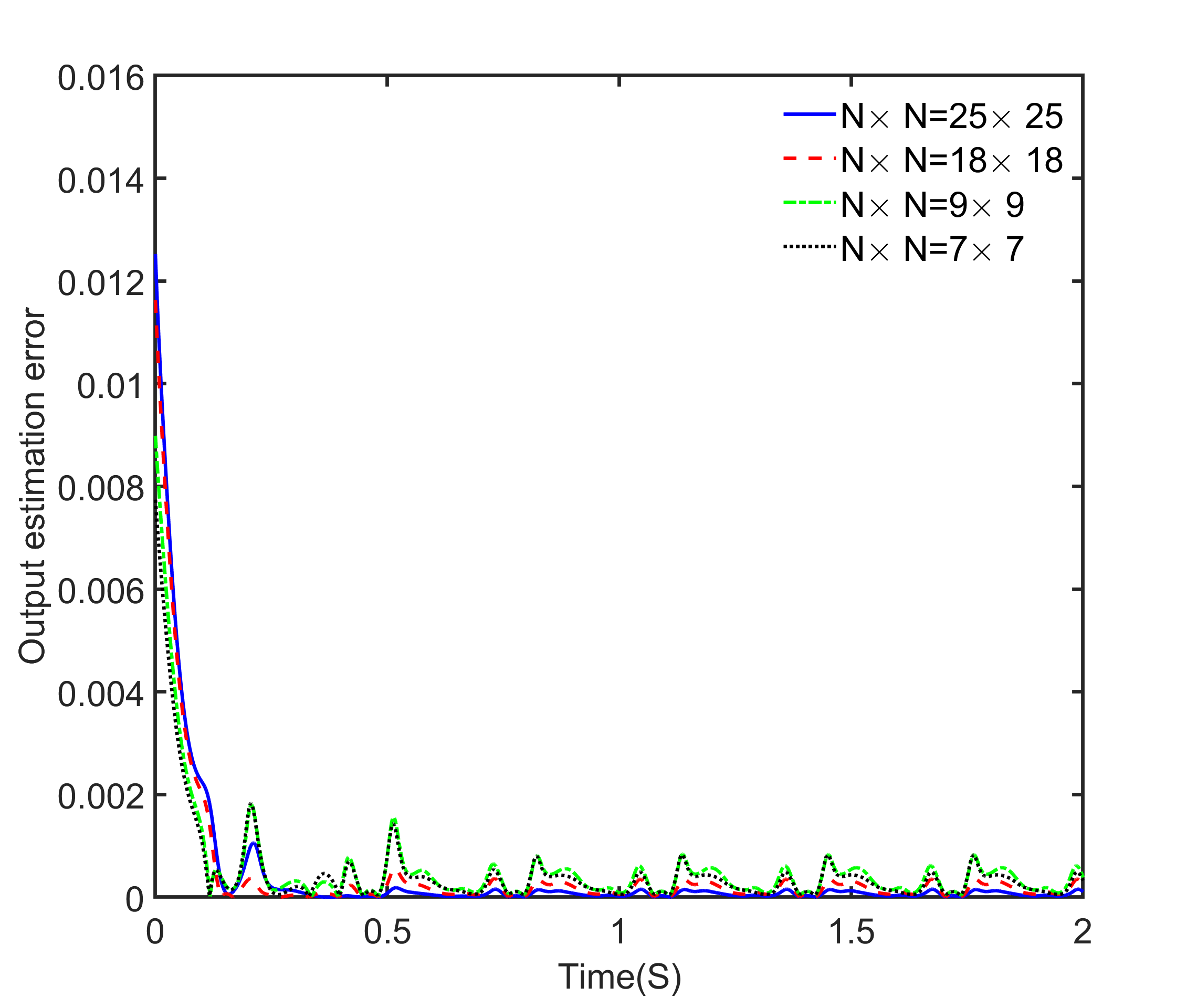
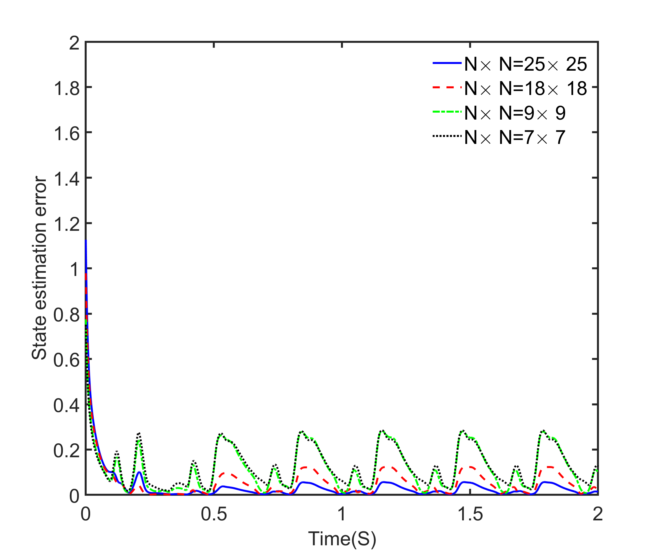
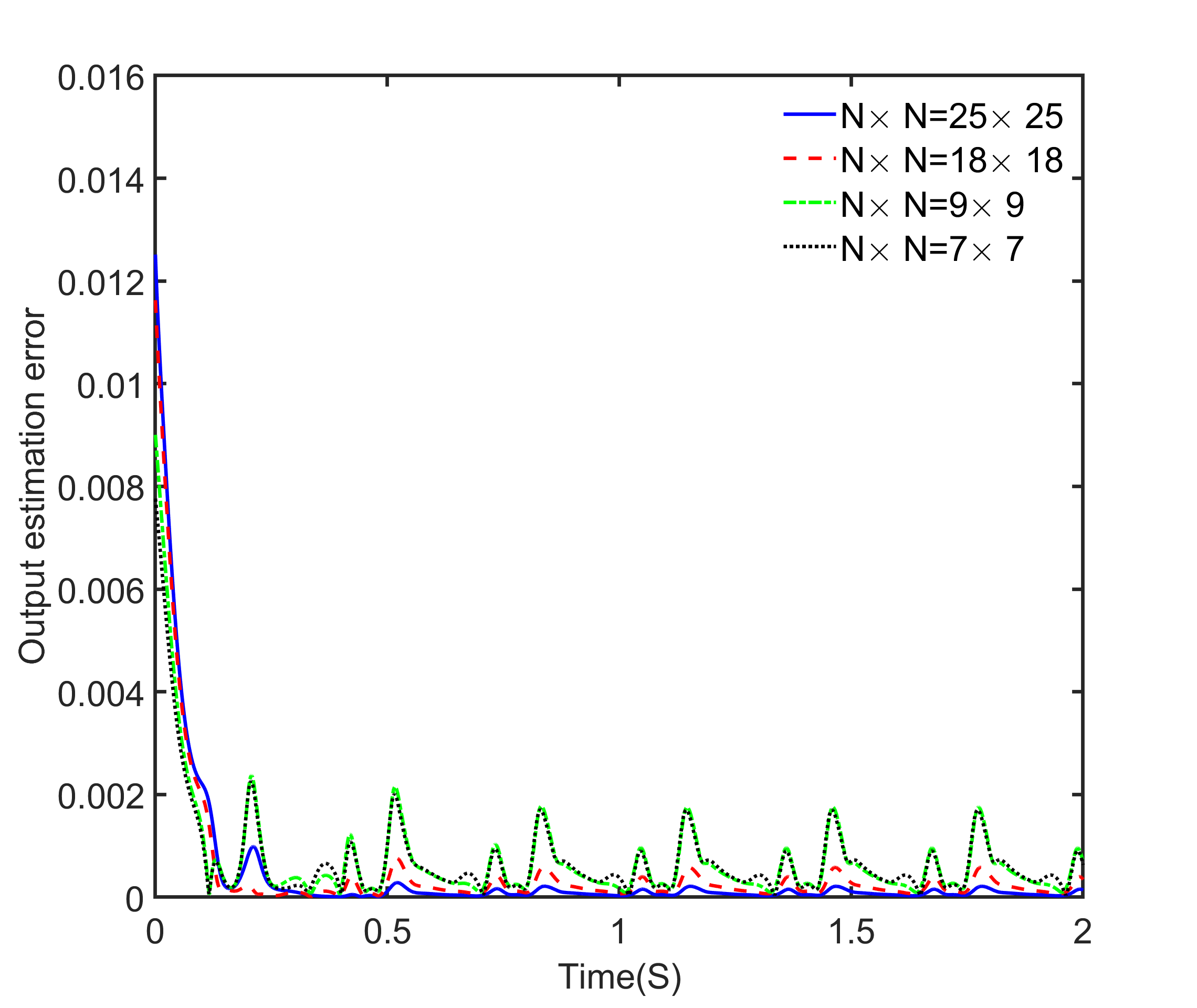
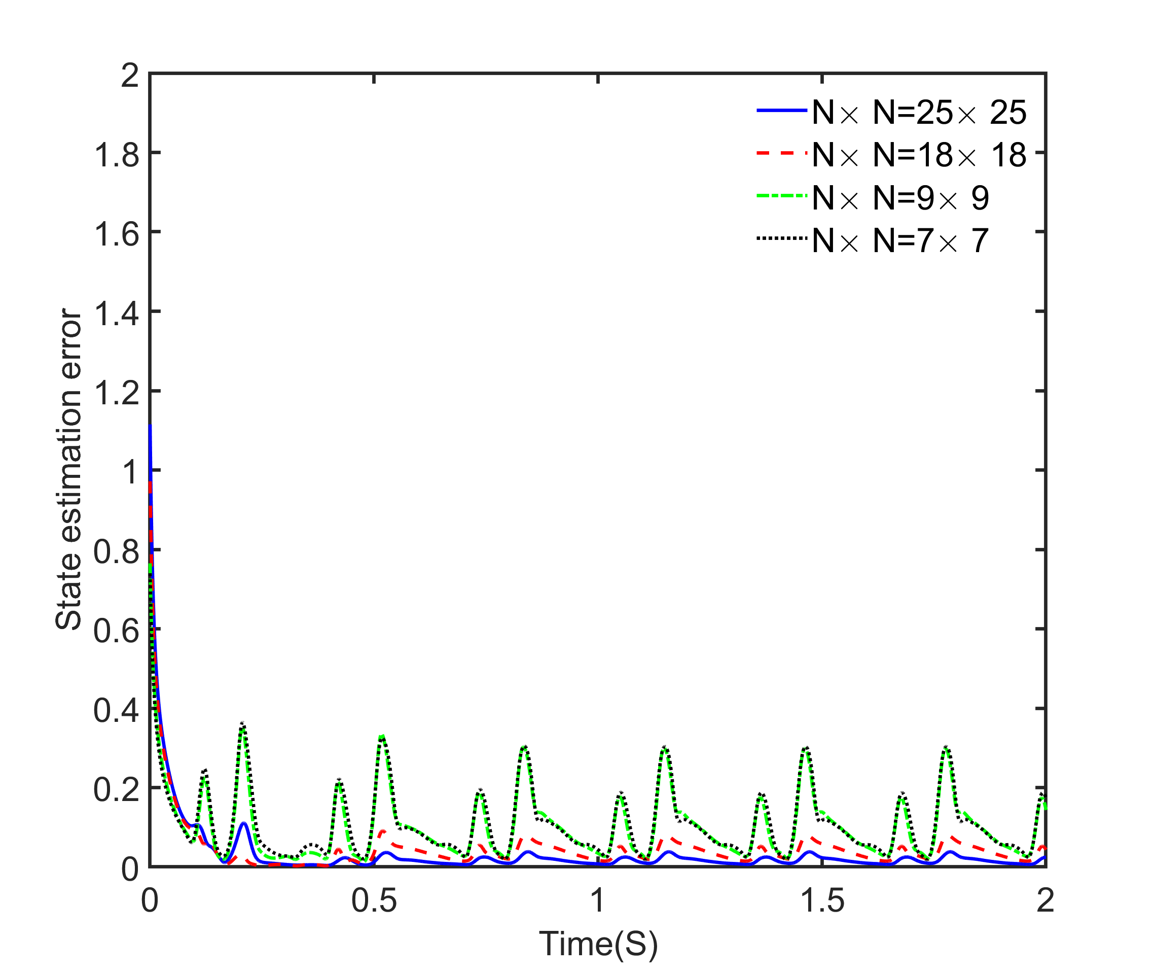
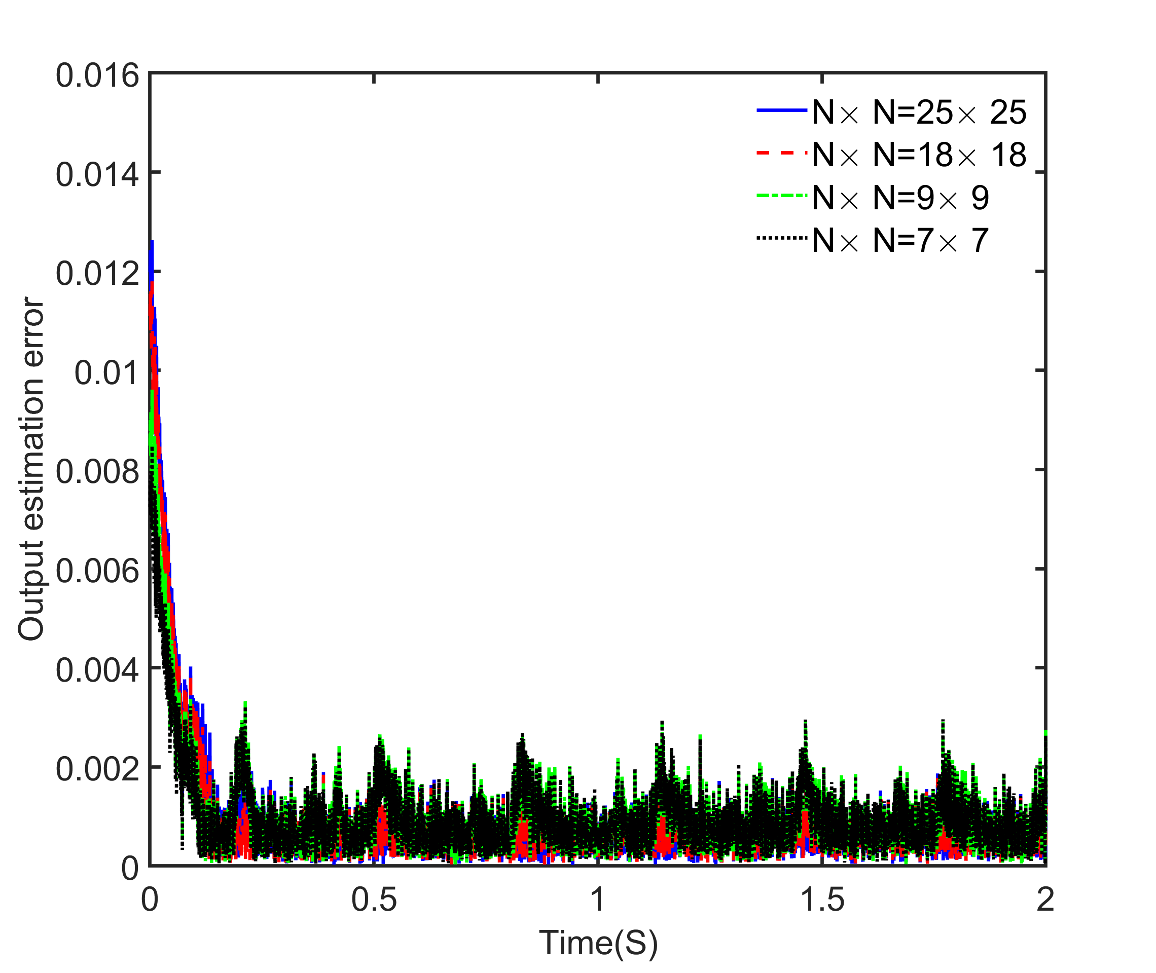
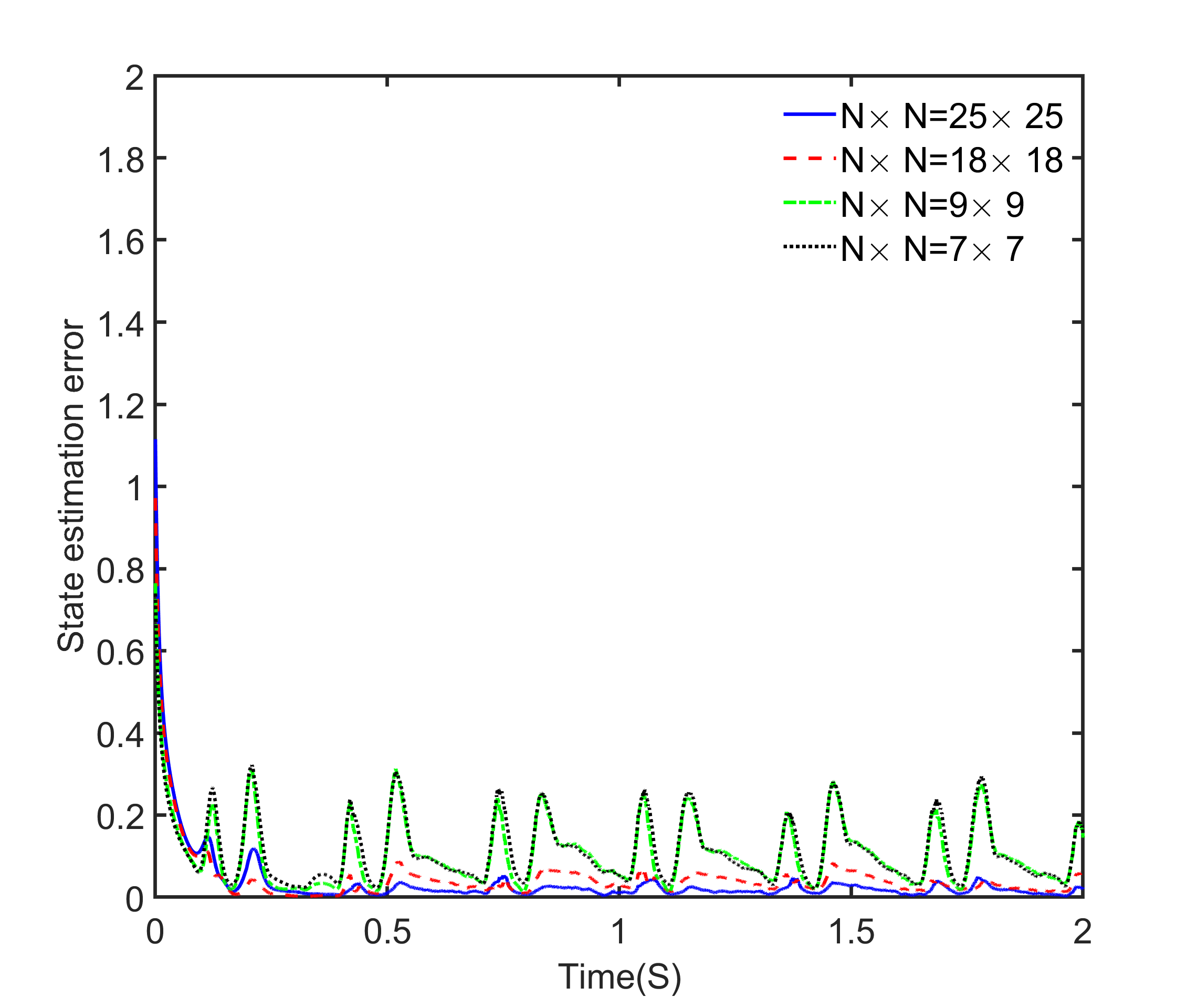
Both system and observer dynamics are approximated using the finite element method with square elements and piecewise linear basis functions. The order of approximation for the system is $35\times 35$. Four different orders of approximation were used for observer dynamics, $25\times 25$, $18\times 18$, $9\times 9$, and $7\times 7$. The equations are solved in MATLAB 2018. The filtering parameters are chosen to be $\alpha=8$, $W(s)=I_{\mathcal{H}}$, and $R(s)=100I_{\mathcal{Y}}$ where $I_{\mathcal{H}}$ and $I_{\mathcal{Y}}$ are the identity operators on $\mathcal{H}$ and $\mathcal{Y}$ respectively. The $L^{2}(\Omega)$-norm of the state estimation error and also the Euclidean norm of the error in the predicted measurement are shown in Figure 3. The errors converge quickly to small values. As expected, the steady-state estimation error increases as the order of the observer decreases.

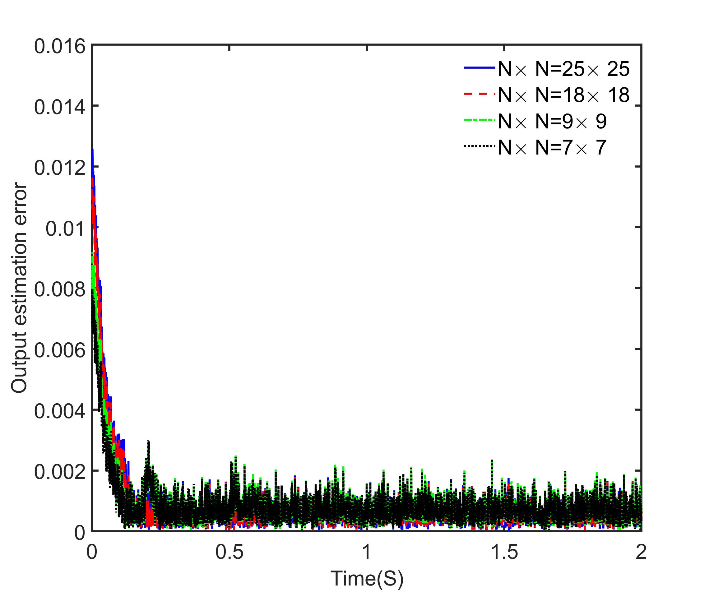
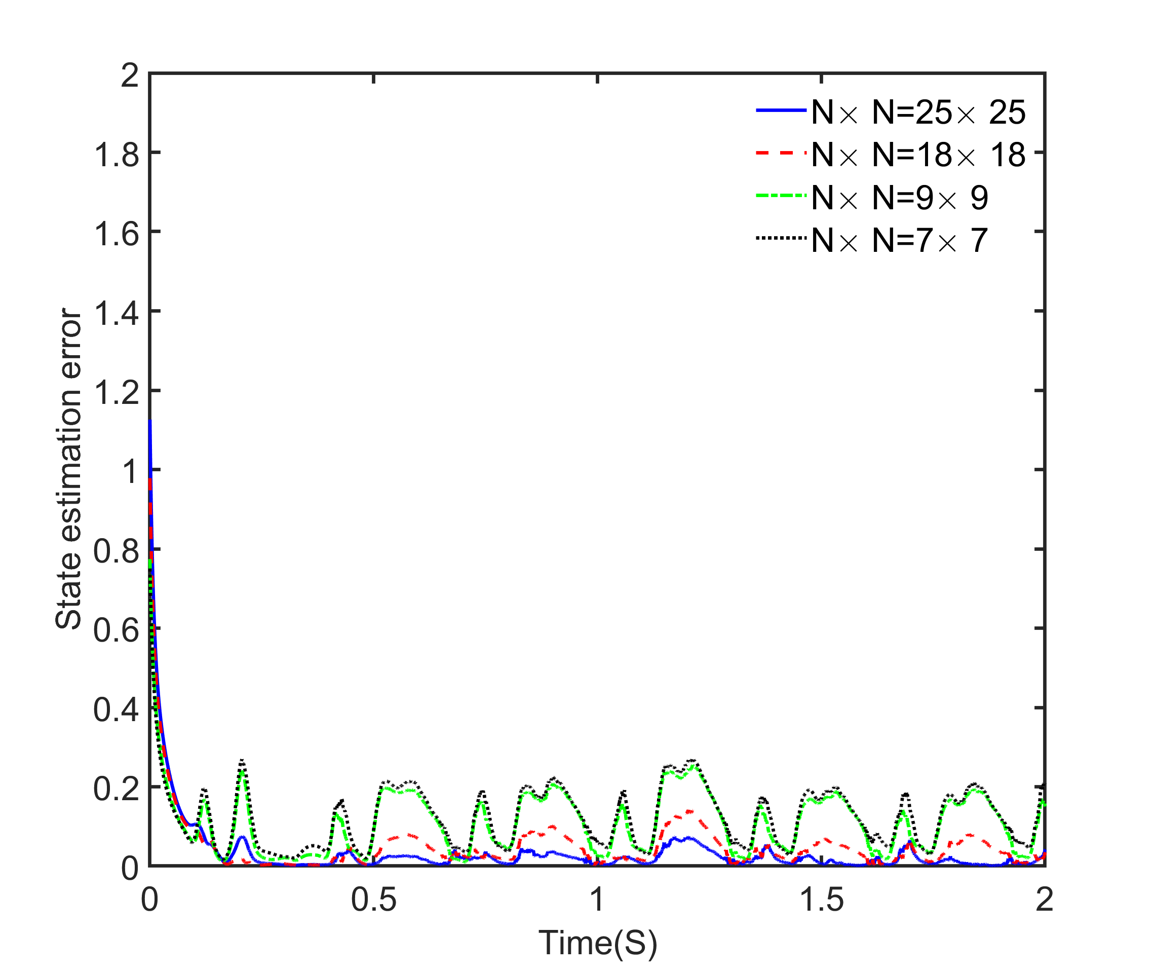
Simulation results in the presence of system and measurement disturbance are shown in Figures 2. The disturbance signal $\omega(t)\in\mathbb{R}$ is generated via MATLAB random signal generator such that it has zero mean and covariance of $0.1$. The output disturbance $\eta(t)\in\mathbb{R}^{3}$ is similarly created with zero mean and a covariance matrix of $\operatorname{diag}(5\times 10^{-3}I_{\mathbb{R}^{2}},5\times 10^{-4})$. The state estimation error increases slightly but remains bounded.

To investigate a less smooth nonlinearity, the velocity field is defined as a function of distribution $V_{f}(t)=\mathds{1}_{2\times 1}c(t)$. The system (79) is reformulated as

$$\dot{c}(t) =-\nabla\cdot(-\mathcal{D}\nabla c(t)+\kappa c^{2}(t)\mathds{1}_{2\times 1}+\kappa cQ_{c}I_{t}(t))+\omega_{1}(t),$$ (82)

$$\dot{I}_{t}(t) =U_{t}(t)+\omega_{2}(t).$$

In this new form, $I_{t}(t)$ is an augmented state so that the state representation of the system follows the form given by (1). Here, $U_{t}(t)$ is the derivative of current vector and is the input to the system; we chose $U_{t}=[0_{1\times 9},0.8\cos(20t),0_{1\times 4},16cos(40t),0_{1\times 30}]^{T}$. The state space is now $\mathcal{H}=\mathcal{L}^{2}(\Omega)\times\mathbb{R}^{m}$ where $m>0$ is the dimension of vector $I_{t}$. The state is $z(t)=(z_{1}(t),z_{2}(t))=(c(t),I_{t}(t))\in L^{2}(\Omega_{s})\times\mathbb{R}^{m}$. Also,

$$Az(t) =\begin{bmatrix}\nabla\cdot(\mathcal{D}\nabla z_{1}(t))&0\\ 0&0\end{bmatrix},$$

$$F(z(t)) =-\nabla\cdot(\kappa z_{1}^{2}(t)\mathds{1}_{2\times 1}+\gamma z_{1}(t)Q_{c}z_{2}(t)),$$

$$Bu(t) =[0,I]^{T}u(t),\quad u(t)=U_{t}(t).$$

The nonlinear function $F(c,I):H^{1}(\Omega)\times\mathbb{R}^{m}\rightarrow\mathcal{H}$ is not Lipschitz continuous over the state space $\mathcal{H}.$

The initial conditions and other details are the same as in the previous example. The error in both the state estimation and in the measurement are shown in Figure 2. Although the assumption of Theorem III.5 on the system nonlinearity is not satisfied, the estimate converges to the true state in these simulations for large-order estimator, and remains small for the lower-order estimators.

In Figures 4, the observer performance in presence of system and output disturbance is shown. The disturbance signal $\omega_{1}(t)\in\mathbb{R}$ and $\omega_{2}(t)\in\mathbb{R}^{4}$ are generated via MATLAB random signal generator such that $\omega(t)=[\omega_{1}(t),\omega_{2}^{T}(t)]^{T}$ has zero mean and a covariance matrix of $0.1I_{\mathbb{R}^{5}}$. The output disturbance $\eta(t)\in\mathbb{R}^{3}$ is similarly created with zero mean and a covariance matrix of $\operatorname{diag}(5\times 10^{-3}I_{\mathbb{R}^{2}},5\times 10^{-4})$. Note that the generated disturbance signals are piece-wise continuous. The estimation error increases compared with the condition with no disturbances. This error increases significantly for lower orders of the observer.

(a)

(b)

Figure 1: Error for different orders of approximation of the observer dynamics (a) ($L^{2}(\Omega)$-norm of state estimation error and (b) Euclidean norm of output estimation error. $V_{f}(t)=[\int_{0}^{r}c^{2}(x,s,t)dx/c(t),\int_{0}^{s}c^{2}(r,y,t)dy/c(t)]^{T}/2$ and $\hat{z}=[0,0]^{T}$.

(a)

(b)

Figure 2: Error for different orders of approximation of the observer dynamics (a) ($L^{2}(\Omega)$-norm of state estimation error and (b) Euclidean norm of output estimation error. $V_{f}(t)=[\int_{0}^{r}c^{2}(x,s,t)dx/c(t),\int_{0}^{s}c^{2}(r,y,t)dy/c(t)]^{T}/2$ and $\hat{z}=[0,0]^{T}$ in presence of system and output disturbance.

(a)

(b)

Figure 3: Error for different orders of approximation of the observer dynamics (a) ($L^{2}(\Omega)$-norm of state estimation error and (b) Euclidean norm of output estimation error. $V_{f}(t)=\mathds{1}_{2\times 1}c(t)$ and $\hat{z}=0$.

(a)

(b)

Figure 4: Error for different orders of approximation of the observer dynamics (a) ($L^{2}(\Omega)$-norm of state estimation error and (b) Euclidean norm of output estimation error. $V_{f}(t)=\mathds{1}_{2\times 1}c(t)$ and $\hat{z}=0$ in presence of system and output disturbance.

VII Conclusion

In this paper, EKF-based observer design for nonlinear finite-dimensional dynamical systems was formally extended to a class of semilinear infinite-dimensional systems. It is not assumed that the system is uniformly observable, so this result is also new for finite-dimensional systems.

The result is illustrated with several examples. In the second example, the nonlinearity is not Lipschitz continuous, but the error appears to be converging to zero. This suggests an extension to a wider class of nonlinearities. Also, since the estimators were of lower order than the approximation used to simulate the system, convergence of finite-dimensional estimators to the infinite-dimensional EKF is suggested.

References

- [1] R. F. Curtain, “A survey of infinite-dimensional filtering,” SIAM Review, vol. 17, no. 3, pp. 395–411, 1975.
- [2] A. Bensoussan, “Some remarks on linear filtering theory for infinite dimensional systems,” in Directions in mathematical systems theory and optimization, ser. Lecture notes in control and information sciences, A. Rantzer and C. I. Byrnes, Eds. Berlin: Springer-Verlag, 2003, vol. 286, pp. 27–39.
- [3] X. Wu, B. Jacob, and H. Elbern, “Optimal control and observation locations for time-varying systems on a finite-time horizon,” SIAM Jour. Control and Optim., vol. 54, no. 1, pp. 291–316, 2015.
- [4] A. Smyshlyaev and M. Krstic, “Backstepping observers for a class of parabolic PDE’s,” Systems & Control Letters, vol. 54, no. 7, pp. 613–625, 2005.
- [5] R. Miranda, I. Chairez, and J. Moreno, “Observer design for a class of parabolic PDE via sliding modes and backstepping,” in 2010 11th International Workshop on Variable Structure Systems (VSS). IEEE, 2010, pp. 215–220.
- [6] R. F. Curtain, “Finite-dimensional compensator design for parabolic distributed systems with point sensors and boundary input,” IEEE Transactions on Automatic Control, vol. 27, no. 1, pp. 98–104, 1982.
- [7] M. A. Demetriou, “Natural second-order observers for second-order distributed parameter systems,” Systems & control letters, vol. 51, no. 3, pp. 225–234, 2004.
- [8] S.-X. Tang, L. Camacho-Solorio, Y. Wang, and M. Krstic, “State-of-charge estimation from a thermal–electrochemical model of lithium-ion batteries,” Automatica, vol. 83, pp. 206–219, 2017.
- [9] S. Tang and M. Krstic, “Observer design for an IPDE with time-dependent coefficients,” in 2016 American Control Conference (ACC). IEEE, 2016, pp. 1655–1660.
- [10] D. Simon, Optimal state estimation: Kalman, H infinity, and nonlinear approaches. John Wiley & Sons, 2006.
- [11] M. S. Grewal and A. P. Andrews, Kalman filtering: theory and practice using MATLAB. John Wiley & Sons, 2011.
- [12] K. Reif and R. Unbehauen, “The extended Kalman filter as an exponential observer for nonlinear systems,” IEEE Transactions on Signal Processing, vol. 47, no. 8, pp. 2324–2328, 1999.
- [13] K. Reif, S. Günther, E. Yaz, and R. Unbehauen, “Stochastic stability of the discrete-time extended Kalman filter,” IEEE Transactions on Automatic Control, vol. 44, 1999.
- [14] ——, “Stochastic stability of the continuous-time extended Kalman filter,” IEEE Proceedings in Control Theory and Applications, 2000.
- [15] X. Kai, C. Wei, and L. Liu, “Robust extended Kalman filtering for nonlinear systems with stochastic uncertainties,” Systems, Man and Cybernetics, Part A: Systems and Humans, IEEE Transactions on, vol. 40, no. 2, pp. 399–405, 2010.
- [16] X. Kai, L. Liangdong, and L. Yiwu, “Robust extended Kalman filtering for nonlinear systems with multiplicative noises,” Optimal Control Applications and Methods, vol. 32, no. 1, pp. 47–63, 2011.
- [17] G. A. Einicke and L. B. White, “Robust extended Kalman filtering,” IEEE Transactions on Signal Processing, vol. 47, no. 9, pp. 2596–2599, 1999.
- [18] D. F. Liang, “Comparisons of nonlinear recursive filters for systems with nonnegligible nonlinearities,” in Control and Dynamic Systems. Elsevier, 1983, vol. 20, pp. 341–401.
- [19] M. I. Ribeiro, “Kalman and extended Kalman filters: Concept, derivation and properties,” Institute for Systems and Robotics, vol. 43, p. 46, 2004.
- [20] S. Elizabeth and R. Jothilakshmi, “Convergence analysis of extended Kalman filter in a noisy environment through difference equations,” International Journal of Differential Equations and Applications, vol. 14, no. 2, 2015.
- [21] F. Alonge, T. Cangemi, F. D’Ippolito, A. Fagiolini, and A. Sferlazza, “Convergence analysis of extended Kalman filter for sensorless control of induction motor,” IEEE Transactions on Industrial Electronics, vol. 62, no. 4, pp. 2341–2352, 2014.
- [22] M. Boutayeb, H. Rafaralahy, and M. Darouach, “Convergence analysis of the extended Kalman filter used as an observer for nonlinear deterministic discrete-time systems,” IEEE transactions on automatic control, vol. 42, no. 4, pp. 581–586, 1997.
- [23] J. Baras, A. Bensoussan, and M. James, “Dynamic observers as asymptotic limits of recursive filters: Special cases,” SIAM Journal on Applied Mathematics, vol. 48, no. 5, pp. 1147–1158, 1988.
- [24] K. Reif, F. Sonnemann, and R. Unbehauen, “An EKF-based nonlinear observer with a prescribed degree of stability,” Automatica, vol. 34, no. 9, pp. 1119–1123, 1998.
- [25] J. H. Ahrens and H. K. Khalil, “Closed-loop behavior of a class of nonlinear systems under EKF-based control,” IEEE Trans. Automat. Control, vol. 52, no. 3, pp. 536–540, 2007.
- [26] H.-N. Wu and H.-X. Li, “ fuzzy observer-based control for a class of nonlinear distributed parameter systems with control constraints,” IEEE Transactions on Fuzzy Systems, vol. 16, no. 2, pp. 502–516, 2008.
- [27] H. N. Wu and H. X. Li, “Robust adaptive neural observer design for a class of nonlinear parabolic PDE systems,” Journal of Process Control, vol. 21, no. 8, pp. 1172–1182, 2011.
- [28] S. Afshar, K. Morris, and A. Khajepour, “A modified sliding-mode observer design with application to the diffusion equation,” International Journal of Control, vol. 92, no. 10, pp. 2369–2382, 2019.
- [29] G. Rigatos, P. Siano, A. Melkikh, and N. Zervos, “Highway traffic estimation using nonlinear Kalman filtering,” Intell Industrial Systems, 2017.
- [30] S. Afshar, K. A. Morris, and A. Khajepour, “State-of-charge estimation using an EKF-based adaptive observer,” IEEE Transactions on Control Systems Technology, 2018.
- [31] R. Miranda, J. Moreno, J. Chairez, and L. Fridman, “Observer design for a class of hyperbolic PDE equation based on a distributed super twisting algorithm,” in 12th International Workshop on Variable Structure Systems (VSS). IEEE, 2012, pp. 367–372.
- [32] M. Bitzer and M. Zeitz, “Design of a nonlinear distributed parameter observer for a pressure swing adsorption plant,” Journal of process control, vol. 12, no. 4, pp. 533–543, 2002.
- [33] M. Efe, H. Özbay, and M. Samimy, “Infinite dimensional and reduced order observers for Burgers equation,” International Journal of Control, vol. 78, no. 11, pp. 864–874, 2005.
- [34] J.-F. Couchouron and P. Ligarius, “Nonlinear observers in reflexive Banach spaces,” ESAIM: Control, Optimisation and Calculus of Variations, vol. 9, pp. 67–103, 2003.
- [35] R. Vazquez, E. Schuster, and M. Krstic, “Magnetohydrodynamic state estimation with boundary sensors,” Automatica, vol. 44, no. 10, pp. 2517–2527, 2008.
- [36] T. Meurer, “On the extended Luenberger-type observer for semilinear distributed-parameter systems,” Automatic Control, IEEE Transactions on, vol. 58, no. 7, pp. 1732–1743, 2013.
- [37] F. Castillo, E. Witrant, C. Prieur, and L. Dugard, “Boundary observers for linear and quasi-linear hyperbolic systems with application to flow control,” Automatica, vol. 49, no. 11, pp. 3180–3188, 2013.
- [38] A. Schaum, J. A. Moreno, E. Fridman, and J. Alvarez, “Matrix inequality-based observer design for a class of distributed transport-reaction systems,” International Journal of Robust and Nonlinear Control, vol. 24, no. 16, pp. 2213–2230, 2014.
- [39] R. Curtain and A. Pritchard, “The infinite-dimensional Riccati equation for systems defined by evolution operators,” SIAM Journal on Control and Optimization, vol. 14, no. 5, pp. 951–983, 1976.
- [40] F. Germ, “Estimation for linear and semi-linear infinite-dimensional systems,” http://hdl.handle.net/10012/14648, University of Waterloo, 2019.
- [41] S. Afshar, F. Germ, and K. Morris, “Well-posedness of extended Kalman filter equations for semilinear infinite-dimensional systems,” in 2020 59th IEEE Conference on Decision and Control (CDC). IEEE, 2020, pp. 1210–1215.
- [42] Z. Denkowski, S. Migorski, and N. S. Papageorgiou, An Introduction to Nonlinear Analysis: Theory. Springer, 2003.
- [43] A. Pazy, Semigroups of Linear Operators and Applications to Partial Differential Equations. Springer, 1983.
- [44] R. F. Curtain and H. Zwart, An introduction to infinite-dimensional linear systems theory. Springer New York, 2020.
- [45] R. F. Curtain, “Estimation theory for abstract evolution equations excited by general white noise processes,” SIAM Journal on Control and Optimization, vol. 14, no. 6, pp. 1124–1150, 1976.
- [46] R. F. Curtain and A. J. Pritchard, Infinite dimensional linear systems theory, ser. Lecture Notes in Control and Information Sciences. Springer-Verlag, Berlin-New York, 1978, vol. 8.
- [47] E. Kreyszig, Introductory Functional Analysis with Applications. Wiley, 1989.
- [48] J. Gibson, “The Riccati integral equations for optimal control problems on Hilbert spaces,” SIAM Journal on Control and Optimization, vol. 17, no. 4, pp. 537–565, 1979.
- [49] R. F. Curtain and H. Zwart, Introduction to infinite-dimensional systems theory. Springer New York, 1995.
- [50] R. Datko, “Uniform asymptotic stability of evolutionary processes in a Banach space,” SIAM Journal on Mathematical Analysis, vol. 3, no. 3, pp. 428–445, 1972.
- [51] A. Mironchenko and C. Prieur, “Input-to-state stability of infinite-dimensional systems: recent results and open questions,” SIAM Review, vol. 62, no. 3, pp. 529–614, 2020.
- [52] S. Afshar, M. B. Khamesee, and A. Khajepour, “Optimal configuration for electromagnets and coils in magnetic actuators,” IEEE Trans. Magn., vol. 49, no. 4, pp. 1372–1381, 2013.
- [53] ——, “Mimo regulation control design for magnetic steering of a ferromagnetic particle inside a fluidic environment,” Internat. J. Control, vol. 88, no. 10, pp. 1942–1962, 2015.
- [54] S. Afshar, “Modeling and control of a magnetic drug delivery system,” Master’s thesis, University of Waterloo, 2012.
- [55] A. Nacev, C. Beni, O. Bruno, and B. Shapiro, “The behaviors of ferromagnetic nano-particles in and around blood vessels under applied magnetic fields,” Journal of magnetism and magnetic materials, vol. 323, no. 6, pp. 651–668, 2011.