Hinge mode dynamics of periodically driven higher-order Weyl semimetals

Abstract

We study the stroboscopic dynamics of hinge modes of a second-order topological material modeled by a tight-binding free fermion Hamiltonian on a cubic lattice in the intermediate drive frequency regime for both discrete (square pulse) and continuous (cosine) periodic drive protocols. We analyze the Floquet phases of this system and show that its quasienergy spectrum becomes almost gapless in the large drive amplitude regime at special drive frequencies. Away from these frequencies, the gapped quasienergy spectrum supports weakly dispersing Floquet hinge modes. Near them, these hinge modes penetrate into the bulk and eventually become indistinguishable from the bulk modes. We provide an analytic, albeit perturbative, expression for the Floquet Hamiltonian using Floquet perturbation theory (FPT) which explains this phenomenon and leads to analytic expressions of these special frequencies. We also show that in the large drive amplitude regime, the zero energy hinge modes corresponding to the static tight-binding Hamiltonian display qualitatively different dynamics at these special frequencies. We discuss possible local density of state measurement using a scanning tunneling microscope which can test our theory.

I Introduction

Topological materials have been a subject of intense theoretical and experimental studies in recent year toporev . The study of these systems began with spin-Hall systems kane05 , topological insulators toporef , and Dirac and Weyl semimetals diracref ; weylref . The key property of these materials which distinguishes them from, for example, trivial insulators, is manifestation of the bulk-boundary correspondence ashwinrev . In these materials, non-trivial topology of the bulk bands results in the presence of symmetry protected surface states. Thus a $d$-dimensional solid hosting a topological phase exhibits topologically protected gapless states localized in its $d-1$ dimensional surface.

More recently, a new class of topological materials, dubbed as higher-order topological materials (HOTMs), have been studied intensively hotmref1 ; hotmref2 ; hotmref3 ; hotmref4 ; hotmref5 ; hotmref6 ; hotmref7 ; hotmref8 ; hotmref9 ; hotmref10 ; hotmref11 ; hotmref12 ; hotmref13 ; hotmref14 ; hotmref15 ; hotmref16 ; hweylref0 ; hweylref1 ; hweylref2 ; hweylref3 ; hweylref4 ; hweylref5 ; hweylref6 ; hweylref7 ; hdiracref1 ; hdiracref2 ; hdiracref3 ; hdiracref4 ; hdiracref5 ; hdiracref6 . A $n^{\rm th}$ order HOTM has non-zero $2^{n}$ moment in the bulk (quadrupole for $n=2$ and octupole for $n=3$) and hosts $d-n$ dimensional topologically protected states on its edges or corners; all other higher dimensional surface modes are gapped out. For example in two-dimensional (2D) second-order topological materials (SOTM), there is a non-zero quadrupole moment in the bulk and the edge states are gapped, while topologically protected states appear at the corner hotmref2 ; hotmref4 ; hotmref5 ; hotmref6 ; hotmref8 ; hotmref9 ; hotmref11 ; hotmref12 ; hotmref13 ; hotmref14 ; hotmref16 . Similarly 3D SOTMs host gapless hinge modes with gapped surface states hotmref4 ; hotmref5 ; hotmref7 ; hotmref9 . A class of such materials include the higher-order Dirac semimetals (HODS) hdiracref1 ; hdiracref2 ; hdiracref3 ; hdiracref4 ; hdiracref5 ; hdiracref6 and the more recently found higher-order Weyl semimetals (HOWS) hweylref0 ; hweylref1 ; hweylref2 ; hweylref3 ; hweylref4 ; hweylref5 ; hweylref6 ; hweylref7 . Apart from the standard Fermi arc states of the typical Weyl semimetals, HOWSs also host gapless hinge states with quantized charge.

The physics of closed quantum systems driven out of equilibrium has also been studied extensively in recent years. rev1 ; rev2 ; rev3 ; rev4 ; rev5 ; rev6 ; rev7 ; rev8 . The quantum dynamics of such systems involving periodic drive protocols are of particular interest; they exhibit a host of phenomena which usually have no counterpart in either equilibrium or aperiodically driven quantum systems ap1 ; ap2 ; ap3 . Such phenomena include dynamical freezing df1 ; df2 ; df3 ; df4 ; df5 , dynamical localization dloc1 ; dloc2 ; dloc3 ; dloc4 , dynamical phase transitions dtran1 ; dtran2 ; dtran3 , presence of time crystalline phases tc1 ; tc2 ; tc3 , and possibility of tuning ergodic properties of a quantum system ergoref . More interestingly, it is realized that such drives can be used to engineer transition between topologically trivial and non-trivial phases of matter topo1 ; topo2 ; topo3 ; topo4 ; topo5 .

In this work, we study a driven tight-binding hopping Hamiltonian for free fermions which is known to host topological Weyl-semimetallic phase in equilibrium hweylref1 . We study this system for continuous and discrete drive protocols. The summary of our main results and their connection to existing ones are charted below.

I.1 Summary of results

The central results that we obtain from our study are as follows.

• First, we chart out the phase diagram of the equilibrium model and demonstrate that it hosts second-order topological phases with a bulk gap and zero energy hinge states. These states serve as initial states in our dynamics studies.

• Second, we use FPT to compute the Floquet Hamiltonian of the driven system corresponding to both discrete square pulse and continuous cosine drive protocols. The Floquet phases obtained from these perturbative analytic Hamiltonians agree remarkably well with that obtained from exact numerics in the large drive amplitude and intermediate frequency regime where second-order Magnus expansion fails.

• Third, we demonstrate the existence of special drive frequencies for which the bulk Floquet spectrum becomes almost gapless. At these frequencies, the first order analytic Floquet Hamiltonian leads to a gapless spectrum; thus the contribution to the gap in the Floquet spectrum comes from higher order terms which are small. This picture is corroborated by exact numerical study of the system which also indicates a drastic reduction of the Floquet spectrum gap at these special frequencies.

• Fourth, we find that the Floquet spectrum supports weakly dispersing hinge modes when the drive frequency is different from these special frequencies. We provide analytic expressions of these hinge states for the discrete protocol for a representative drive frequency starting from the perturbative first order Floquet Hamiltonian; we find the analytic expressions to be qualitatively similar to those obtained from exact numerics. In contrast, the hinge modes of the Floquet spectrum delocalizes into the bulk and becomes almost indistinguishable from the bulk modes at these special drive frequencies.

• Fifth, we study the manifestation of such a small bulk Floquet gap on the dynamics of the hinge modes. Starting from an initial zero energy eigenstate of the equilibrium Hamiltonian which is localized at one of the hinges, we show, by computing the spatially resolved probability distribution of the driven hinge state, that the dynamics keeps the state localized to the initial hinge when the bulk Floquet gap is large. In contrast, at the special drive frequencies where the bulk Floquet gap becomes small, the hinge modes show coherent propagation between diagonally opposite hinges with a fixed periodicity. We provide an analytic estimate of this periodicity using the first order perturbative Floquet Hamiltonian.

• Finally, we point out that such a periodic variation would reflect in the local density of state (LDOS) of the fermions and is hence measurable by a scanning tunneling microscope (STM). This allows for the possibility of verification of our theoretical results in standard STM experiments.

I.2 Comparison with existing works

Most of the theoretical efforts in the direction of Floquet engineering of HOTMs have been based on either a class of hopping Hamiltonians on specific lattices hotmbandcontref1 ; hotmbanddiscrref2 ; hotmbanddiscrref3 ; hotmbanddiscrref4 ; hotmbandcontref5 ; hotmbanddiscrref6 ; hotmbanddiscrref7 ; hotmbanddiscrref8 ; hotmbanddiscrref9 ; hotmbanddiscrref10 ; hotmbanddiscrref11 or driven topological superconductors hotmsupdiscrref1 ; hotmsupcontref2 ; hotmsupcontref3 ; hotmsupcontref4 ; hotmsupdiscrref5 ; hotmsupdiscrref6 ; hotmsupdiscrref7 ; hotmsupdiscrref8 . The drive protocols followed in these studies are either continuous arising from interaction of such systems with light hotmbandcontref1 ; hotmbandcontref5 ; hotmsupcontref2 ; hotmsupcontref3 ; hotmsupcontref4 ; hotmsupdiscrref8 or specifically engineered discrete ones where one of the Hamiltonian parameters are changed discontinuously with time hotmbanddiscrref2 ; hotmbanddiscrref3 ; hotmbanddiscrref4 ; hotmbanddiscrref6 ; hotmbanddiscrref7 ; hotmbanddiscrref8 ; hotmbanddiscrref9 ; hotmbanddiscrref10 ; hotmbanddiscrref11 ; hotmsupdiscrref1 ; hotmsupdiscrref5 ; hotmsupdiscrref6 ; hotmsupdiscrref7 ; hotmsupdiscrref8 . These studies clearly establish that such periodic driving can be used to engineer higher-order topological Floquet phases even when the ground state of the equilibrium parent Hamiltonian do not host such a phase. The theoretical analysis leading to this result may be classified into two distinct categories. The first involves construction of exact Floquet unitaries for discrete protocols followed by their numerical analysis to unravel the existence of the higher-order Floquet phase hotmsupdiscrref5 ; hotmsupdiscrref6 ; hotmsupdiscrref7 . The second class of studies, carried out for both discrete and continuous protocols, involves analytic computation of the Floquet Hamiltonian of the system in the high-frequency regime using perturbation techniques which uses $T$ as the expansion parameter hotmbandcontref1 ; hotmbanddiscrref2 ; hotmbanddiscrref3 ; hotmsupdiscrref1 . The latter class provide analytic insight into the properties of the Floquet Hamiltonian only in the high-frequency regime where such low $T$ expansions are accurate. To the best of our knowledge, such studies have not been extended to the intermediate frequency regime where these perturbative methods fail. Our study, on the other hand, uses FPT to explore this intermediate frequency regime both analytically and numerically. In the process, we encounter features like dispersion of hinge modes and closing of bulk band gap, which have no analogue both in the undriven and in the high frequency driven version. As we discuss in detail in Sec. IV.3, this closing of the band gap, in addition to being an artifact of the first order theory, doesn’t lead to a change in topology, as this isn’t accompanied by a band inversion. Nevertheless, this leaves dynamical signatures, which serve as diagnostic tools of our Floquet phases. To the best of our knowledge, such diagnosis of Floquet phases has not been discussed in the literature so far.

The plan of the rest of the work are as follows. In Sec. II, we define the starting Hamiltonian and chart out its equilibrium phase diagram. This is followed by Sec. III where we derive the analytic, albeit perturbative, Floquet Hamiltonian using FPT for both discrete and continuous drive protocols. Next, in Sec. IV, we discuss the Floquet phases and compare the FPT results with those from exact numerics. This is followed by Sec. V where we discuss the dynamics of the hinge modes. Finally we discuss our main results and conclude in Sec. VI. A derivation of the Floquet Hamiltonian for both continuous and discrete protocol using Magnus expansion is presented in the appendix.

II Model Hamiltonian and Equilibrium Phases

We begin with the low-energy model tight-binding Hamiltonian on a cubic lattice involving four spinless fermions within an unit cell hosting higher-order Weyl semimetal phases hweylref1 . A schematic picture of the model is shown in the top left panel of Fig. 1. In momentum-space, the Hamiltonian of this system is given by

$$H = \sum_{\vec{k}}\psi_{\vec{k}}^{\dagger}H_{0}(\vec{k})\psi_{\vec{k}}$$

$$H_{0}(\vec{k}) = a_{4}\Gamma_{1}+a_{2}\Gamma_{2}+a_{3}\Gamma_{3}+a_{1}\Gamma_{4}+ia_{5}\Gamma_{2}\Gamma_{3},$$

$$a_{1(2)} = (\gamma_{z}+\lambda\cos k_{x(y)}),\quad\gamma_{z}=\gamma_{0}+\frac{\lambda}{2}\cos k_{z},$$

$$a_{3(4)} = \lambda\sin k_{x(y)},\quad a_{5}=m_{0}\sin k_{z},$$ (1)

where $\psi_{k}$ denotes a four-component annihilation operator for fermions, the lattice spacing has been set to unity, $\gamma_{0}$($\lambda)$ denotes intra-(inter-)cell hopping amplitudes as shown in Fig. 1, $\vec{k}=(k_{x},k_{y},k_{z})$ indicates crystal momenta, and the matrices $\Gamma_{\mu}$ are given, in terms of outer product of two Pauli matrices $\tau$ and $\sigma$, by

$$\Gamma_{\alpha} = -\tau_{y}\otimes\sigma_{\alpha},\,\,\Gamma_{0}=\tau_{z}\otimes I_{\sigma},\,\,\Gamma_{4}=\tau_{x}\otimes I_{\sigma}.$$ (2)

Here $I_{\tau}$ and $I_{\sigma}$ denote $2\times 2$ identity matrices and the index $\alpha$ takes values $1,2,3$. The matrices $\Gamma_{\mu}$ satisfies the commutation relation $\{\Gamma_{\mu},\Gamma_{\nu}\}=2\delta_{\mu\nu}I_{\tau}\otimes I_{\sigma}$.

The model in Eq. (1) preserves inversion $\mathcal{I}=I_{\tau}\otimes\sigma_{y}$ and mirror $M_{y}=\tau_{x}\otimes\sigma_{x}$ symmetries, while time-reversal $T_{0}=\mathcal{K}$ (where ${\mathcal{K}}$ denotes complex conjugation), the four-fold rotational symmetry $C_{4}^{z}$ and mirror along $x$, $M_{x}=\tau_{x}\otimes\sigma_{z}$, are broken. In addition, the model preserves $M_{x}T_{0}$. We note that for the model $M_{z}$ is defined through ${\mathcal{I}}=M_{x}M_{y}M_{z}$ and that for $m_{0}=0$, $H_{0}$ preserves $C_{4}^{z}$ along with other symmetries mentioned above and hosts a higher-order topological semimetal phase.

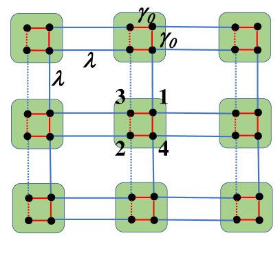
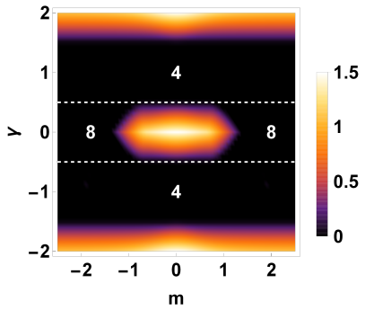
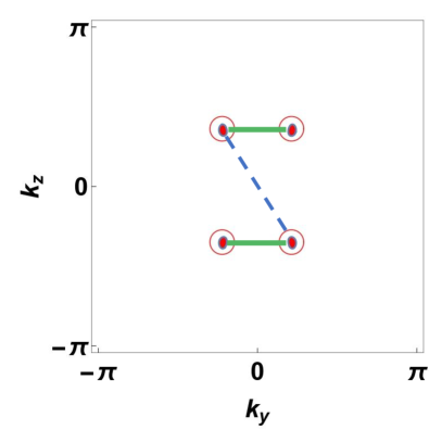
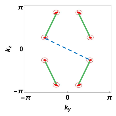
Figure 1: Top Panel: Left: A lattice realization of a two-dimensional quadrapolar insulator (QI) with four orbitals as indicated by 1-4 numbers. The 3D structure is obtained by stacking 2D QIs. The red and blue lines denote intra-cell and inter-cell hopping, respectively. Right: Plot of the bulk bandgap as obtained from Eq. (3) for different values of $\gamma$ and $m$. The black regime is gapless with 4 or 8 Weyl nodes as indicated and the rest including the central hexagon-like regime are gapped. Bottom Panel: The location of Weyl points for $\gamma=-1.0$ (left) and $m=0.75$ and $\gamma=-0.2$ and $m=2.0$ (right). The green solid and blue dashed lines are schematic representations of the surface and hinge arcs respectively. All energies are scaled in units of $\lambda$ and the circles for plots in the bottom panels are guide to the eye.

The energy spectrum of Eq. (1) is given by

$$E_{\pm,\pm} = \pm\sqrt{\sum_{i=1,5}a_{i}^{2}\pm 2|a_{5}|\sqrt{a_{1}^{2}+a_{4}^{2}}},$$ (3)

where $E_{+-}$ and $E_{--}$ correspond to the lowest conduction and highest valence band respectively. For Fermi energy $\epsilon_{F}=0$, the band spectrum in Eq. (3) can be gapped or gapless depending on the dimensionless parameters $\gamma=\gamma_{0}/\lambda$ and $m=m_{0}/\lambda$. It is evident from the top right panel of Fig. 1 that the spectrum is gapless for $-1.5\leq\gamma\leq 1.5$ except the central hexagonal-like regime, satisfying $|\gamma|\leq 0.5$ and

$$|m| \leq \sqrt{(1-|\gamma|)+\frac{1}{2}\sqrt{3-8|\gamma|+4\gamma^{2}}},$$ (4)

where the spectrum is gapped.

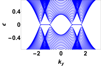
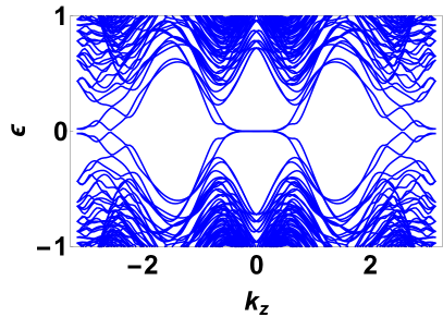
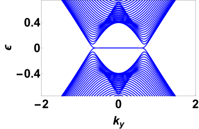
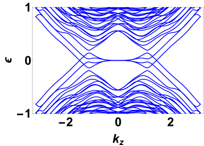
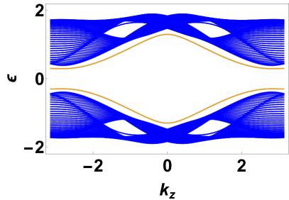
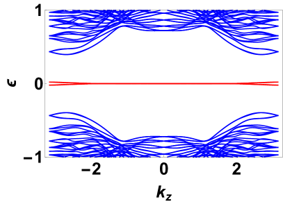
Figure 2: Top Panels: Left: Plot of surface Fermi arc of undriven Hamiltonian (Eq. (1)) as a function of $k_{y}$ with open boundary condition (OBC) along $z$ and $k_{x}=0$ for gapless bulk regime with eight Weyl nodes ($\gamma=-0.2,\text{ }m=2.0$). Right: The gapless hinge mode is obtained as a function of $k_{z}$ with OBC along $x$ and $y$ with the same parameter set. It connects two middle node at $k_{z}=0$. Middle Panels: Same as the corresponding top panels but for gapless bulk with four Weyl nodes ($\gamma=-1.0,\text{ }m=0.75$). Bottom panels: Left: Energy spectrum for gapped bulk ($\gamma=-0.2$, $m=0.4$) as a function of $k_{z}$ with $k_{x}=0$ and OBC along $y$. The surface localized modes, indicated by orange solid lines, are gapped. Right: The hinge mode, obtained with OBC along $x$ and $y$ denoted by red line is gapless, reflecting the typical quadrupolar insulating phase.

The gapless regime can further be divided into two regimes based on the number of Weyl nodes. Note that the Weyl nodes in this particular model lie in the $k_{y}-k_{z}$ plane (bottom panels of Fig. 1) (instead of the high symmetric lines $k_{x}=0$ and $k_{y}=0$). The gapless regime with $|\gamma|<0.5$ exhibits eight Weyl nodes which are connected through surface Fermi arc along the $z$-surface, as shown in the top left panel of Fig. 2. A further cut of this surface either along $x$ or $y$ does not give rise to any hinge mode. Instead, the hinge mode exists along $k_{z}$, connecting two Weyl nodes closest to $k_{z}=0$ as depicted in the top right panel of Fig. 2. Thus the hinge and surface modes are perpendicular to each other in the present model . As we move away from $|\gamma|<0.5$ to $|\gamma|\geq 0.5$, four Weyl nodes annihilate in pairs while the rest four retain. As before, we find gapless surface and hinge modes connecting Weyl nodes at the center of momenta $k_{y}=0$ and $k_{z}=0$, respectively (center left and right panels of Fig. 2). Finally, for the central hexagonal-like regime with $|\gamma|<0.5$ shown in the right panel of Fig. 1, all Weyl nodes annihilate in pairs, resulting in gapped insulating phase. In this regime, the surface bands denoted by orange solid line in the bottom left panel of Fig. 2 are gapped, whereas the hinge mode is found to be gapless (see bottom right panel Fig. 2), indicating the standard quadrupolar topological insulating (QTI) phase.

III Floquet Perturbation theory

The studies of topological properties of a periodically driven closed quantum system relies on computation of its Floquet Hamiltonian $H_{F}$ which is related to its unitary evolution operator $U(T,0)$ via the relation rev8

$$U(T,0) = {\mathcal{T}}_{t}\left[e^{-i\int_{0}^{T}H(t)dt/\hbar}\right]=e^{-iH_{F}T/\hbar},$$ (5)

where ${\mathcal{T}}_{t}$ denotes time ordering, $T=2\pi/\omega_{D}$ is the time period of the drive, $\omega_{D}$ is the drive frequency, and $\hbar$ is Planck’s constant. The knowledge of $H_{F}$ allows one to compute Floquet eigenstates; it is well known that they host non-trivial topological properties exhibiting transitions from trivial to non-trivial topological phases as a function of the drive frequency. It is well known that a driven system may host such topological phases and associated transitions between them even when the corresponding equilibrium Hamiltonian is topologically trivial topo1 ; topo2 ; topo3 ; topo4 ; topo5 .

The exact computation of the Floquet Hamiltonian for a generic quantum system is difficult; one therefore relies on several perturbative method for its computation rev8 ; flrev . One such perturbative scheme is the Magnus expansion where $T$ is taken as the perturbation parameter. However, the convergence of such an expansion is difficult to ascertain; moreover, it almost always fails to provide qualitatively accurate results in the intermediate or low frequency regimes. In contrast, the properties of $H_{F}$ in the intermediate drive frequency regime is known to be well-described by the Floquet perturbation theory which uses the inverse of the drive amplitude as the perturbation parameter dsenref ; cooperref ; roopayanref .

In this section, we shall provide an analytic computation of the Floquet Hamiltonian of the model in the presence of a periodic drive which is implemented by making $\gamma$ a periodic function of time: $\gamma(t)=\gamma_{0}+\gamma_{1}(t)$ using Floquet perturbation theory (for a review of this method, see Ref. rev8, ). The precise time dependence of $\gamma_{1}(t)$ depends on the protocol. In this section, we shall study two such protocols. The first, which constitutes a square pulse, leads to

$$\gamma_{1}(t)=\begin{cases}-\gamma_{1},&0\leq t<\frac{T}{2}\\ \gamma_{1},&\frac{T}{2}\leq t\leq T,\end{cases}$$ (6)

where $\gamma_{1}$ is the amplitude of the pulse and $T$ denotes its time period. The second constitutes a continuous protocol for which

$$\gamma_{1}(t)=\gamma_{1}\cos\omega_{D}t.$$ (7)

For implementing the FPT, we write $H(t)=H_{0}+H^{\prime}(t)$, where

$$H^{\prime}(t)=\gamma_{1}(t)(\Gamma_{2}+\Gamma_{4}).$$ (8)

Note that $H^{\prime}(t)$ does not break any of the additional symmetries discussed earlier.

We focus on the regime of large drive amplitude, i.e., $\gamma_{1}\gg\gamma_{0},\lambda,m_{0}$. In this case, we can treat $H^{\prime}(t)$ exactly and $H_{0}$ perturbatively to find the Floquet unitary and hence $H_{F}$. The first term in such an expansion constitutes the unitary evolution operator $U_{0}(t,0)$ given by

$$U_{0}(t,0) = {\mathcal{T}}_{t}\exp\left[\frac{-i}{\hbar}\int_{0}^{t}dt^{\prime}H^{\prime}(t^{\prime})\right].$$ (9)

For the square pulse protocol given by Eq. 6, this yields

$$U_{0}^{(s)}(t,0) = \exp[i\gamma_{1}t(\Gamma_{2}+\Gamma_{4})/\hbar]\quad 0\leq t\leq T/2,$$

$$= \exp[i\gamma_{1}(T-t)(\Gamma_{2}+\Gamma_{4})/\hbar]\quad T/2\leq t\leq T,$$

which yields $U_{0}^{(s)}(T,0)=I$ and $H_{F}^{(0;s)}=0$. For the continuous drive protocol given by Eq. 7, one gets

$$U_{0}^{(c)} = \exp\left[-\frac{i\gamma_{1}\sin\omega_{D}t}{\omega_{D}\hbar}(\Gamma_{2}+\Gamma_{4})\right]$$ (11)

which also yields $H_{F}^{(0;c)}=0$.

Next we consider the first order term in the Floquet perturbation theory which is given by

$$U_{1}(T,0) = \frac{-i}{\hbar}\int_{0}^{T}U_{0}^{\dagger}(t,0)H_{0}U_{0}(t,0),$$

$$H_{F}^{(1)} = \frac{i\hbar}{T}U_{1}(T,0).$$ (12)

A straightforward calculation using Eqs. 1 and III yields for the square pulse protocol

$$H_{F}^{(1);s}= \frac{1}{2}\left((a_{1}+a_{2})(\Gamma_{4}+\Gamma_{2})+ia_{5}(\Gamma_{2}\Gamma_{3}+\Gamma_{3}\Gamma_{4})\right)+\frac{\hbar\sin{(\sqrt{2}\gamma_{1}T/\hbar)}}{2\sqrt{2}\gamma_{1}T}\left((a_{1}-a_{2})(\Gamma_{4}-\Gamma_{2})+ia_{5}(\Gamma_{2}\Gamma_{3}-\Gamma_{3}\Gamma_{4})\right)$$

$$+i\frac{\hbar(\cos{(\sqrt{2}\gamma_{1}T/\hbar)}-1)}{2\gamma_{1}T}\left((a_{1}-a_{2})\Gamma_{2}\Gamma_{4}+(\Gamma_{2}+\Gamma_{4})(a_{3}\Gamma_{3}+a_{4}\Gamma_{1})+ia_{5}\Gamma_{3}\right)+\frac{\hbar\sin{(\sqrt{2}\gamma_{1}T/\hbar)}}{\sqrt{2}\gamma_{1}T}(a_{3}\Gamma_{3}+a_{4}\Gamma_{1}).$$ (13)

Note that the symmetries of the undriven Hamiltonian is retained in the effective Floquet Hamiltonian $H_{F}^{(1);s}$. A similar calculation for the continuous protocol using Eqs. 1 and 11 yields

$$H_{F}^{(1);c} = \frac{1}{2}\left[(a_{1}+a_{2})(\Gamma_{2}+\Gamma_{4})+ia_{5}(\Gamma_{2}\Gamma_{3}+\Gamma_{3}\Gamma_{4})\right]+\mathcal{J}_{0}\left(\frac{\sqrt{2}\gamma_{1}T}{\hbar\pi}\right)\Big{[}a_{3}\Gamma_{3}+a_{4}\Gamma_{1}+\frac{1}{2}((a_{1}-a_{2})(\Gamma_{4}-\Gamma_{2})$$ (14)

$$+ia_{5}(\Gamma_{2}\Gamma_{3}-\Gamma_{3}\Gamma_{4}))\Big{]},$$

where $J_{0}$ denotes zeroth order Bessel function of the first kind and we have used the identity $\exp[i\alpha\sin x]=\sum_{n}J_{n}(\alpha)\exp[inx]$.

We note that for the square pulse protocol $H_{F}^{(1);s}$ takes a particularly simple form around $\sqrt{2}\gamma_{1}T/\hbar=2n\pi$ (for $n\neq 0\in Z$) where only the first term in Eq. 13 survives. We shall see in Sec. IV.3 that this leads to presence of ring of Weyl nodes in the spectrum of $H_{F}^{(1);s}$. A similar simplification occurs for the continuous drive protocol at $\sqrt{2}\gamma_{1}T=\pi\alpha_{n}$, where $\alpha_{n}$ denotes the position of the $n^{\rm th}$ zero of the Bessel function. These features, for either square pulse or continuous protocols, are difficult to obtain within a Magnus expansion as shown via explicit calculation in the appendix; in fact, it can be shown that our results in Eqs. 13 and 14 constitute an infinite re-summation of a class of terms in the Magnus expansion ergoref .

Next, we compute the second order terms in the perturbative expansion. The expression for such terms can be written, in terms of $H_{0}(t)=U_{0}^{\dagger}(t,0)H_{0}U_{0}(t,0)$ as

$$U_{2}(T,0) = \left(\frac{-i}{\hbar}\right)^{2}\int_{0}^{T}dt_{1}H_{0}(t_{1})\int_{0}^{t_{1}}dt_{2}H_{0}(t_{2}),$$

$$H_{F}^{(2)} = \frac{i\hbar}{T}\left(U_{2}(T,0)-\frac{1}{2}U_{1}^{2}(T,0)\right).$$ (15)

For the square pulse protocol given by Eq. 6, it turns out that $U_{0}(t,0)=U_{0}(T-t,T/2)$ for all $t\leq T/2$. It can be shown that this symmetry allows one to write

$$U_{2}^{s}(T,0)=2\left(\frac{-i}{\hbar}\right)^{2}\int_{0}^{T/2}dt_{1}H_{0}(t_{1})\int_{0}^{T/2}dt_{2}H_{0}(t_{2}),$$ (16)

thereby implying that $U_{2}^{s}(T,0)=\frac{1}{2}[U_{1}^{s}(T,0)]^{2}$. Thus the second order correction, $H_{F}^{(2);s}$, vanishes identically. So for the square pulse protocol, $H_{F}^{(1);s}$ provides the Floquet Hamiltonian up to third order in perturbation theory.

The symmetry property mentioned above does not hold for the continuous protocol given in Eq. 7. In this case one obtains a finite contribution to the second order Floquet Hamiltonian. The computation is straightforward, though somewhat cumbersome. The final result is

$$H_{F}^{(2);c} = -\frac{1}{\sqrt{2}}\sum_{n=-\infty}^{\infty}\frac{\mathcal{J}_{2n+1}\left(\frac{\sqrt{2}\gamma_{1}T}{\hbar\pi}\right)}{(2n+1)\hbar\omega_{D}}\Big{[}\left((a_{1}^{2}-a_{2}^{2}+a_{5}^{2})(\Gamma_{2}-\Gamma_{4})-2(a_{1}+a_{2})(a_{3}\Gamma_{3}+a_{4}\Gamma_{1})-2ia_{1}a_{5}(\Gamma_{2}+\Gamma_{4})\Gamma_{3}\right.$$ (17)

$$\left.+2ia_{3}a_{5}\Gamma_{2}\Gamma_{4}\right)+\mathcal{J}_{0}\left(\frac{\sqrt{2}\gamma_{1}T}{\hbar\pi}\right)\left(\left((a_{1}-a_{2})^{2}+a_{5}^{2}+2(a_{3}^{2}+a_{4}^{2})\right)(\Gamma_{2}+\Gamma_{4})+2ia_{1}a_{5}(\Gamma_{2}-\Gamma_{4})\Gamma_{3}\right)\Big{]}.$$

We note that for $\hbar\omega_{D}\sim{\rm O}(\gamma_{1})$, the second order Floquet terms are suppressed by a factor of ${\rm O}(1/\gamma_{1})$; thus in this regime, we expect the first order term to be reasonably accurate.

Before closing this section, we note that the presence of such gapless first order Floquet Hamiltonian implies that at least at the high-frequency regime, the exact Floquet Hamiltonian will at most have a tiny gap in its spectrum. This is due to the fact that such a gap can only originate from higher order terms which are small in the high-frequency regime. We shall discuss this issue and its implication for the hinge modes of the model in more details in Secs. IV and V.

IV Floquet Phases

In this section, we analyze the spectrum of $H_{F}^{(1)}$ in the intermediate and high-frequency regime and compare the result with those obtained from numerical computation of exact $H_{F}$. For the sake of concreteness, we shall mainly focus on the regime where $H(t=0)$ hosts a quadrupolar insulating ground state. In Sec. IV.1, we discuss the Floquet phases of the model. This is followed by analysis of the properties of $H_{F}$ for some special drive frequencies in Secs. IV.2 and IV.3.

IV.1 The bulk spectrum

The computation of the exact Floquet Hamiltonian, which shall be used for obtaining the Floquet phases, can be carried out as follows. For the square pulse protocol, we write the Hamiltonian $H[\gamma=\gamma_{0}\pm\gamma_{1}]=H_{\pm}$. In terms of $H_{\pm}$, one can write the evolution operator as

$$U_{s}^{\rm ex}(T,0) = e^{-iH_{+}T/(2\hbar)}e^{-iH_{-}T/(2\hbar)}.$$ (18)

To evaluate $U_{s}^{\rm ex}$, we first obtain the eigenvalues and eigenvectors of $H_{\pm}$. This can be done analytically for periodic boundary condition, but needs to be done numerically for open boundary condition. We use the latter here for extracting the properties of the Floquet phases. We define the corresponding eigenvalues and eigenvectors as $\epsilon_{n}^{\pm}$ and $|n^{\pm}\rangle$. In the basis of these eigenstates $U_{s}^{\rm ex}(T,0)$ can be written as

$$U_{s}^{\rm ex}(T,0) = \sum_{n_{+},m_{-}}e^{-i(\epsilon_{n}^{+}+\epsilon_{m}^{-})T/(2\hbar)}c^{-+}_{mn}|m^{-}\rangle\langle n^{+}|.$$ (19)

The diagonalization of $U_{s}^{\rm ex}$ in this basis leads to the eigenvalues $\lambda_{p}=e^{i\theta_{p}}$ and the corresponding eigenvectors $|p\rangle$. The exact Floquet eigenvalues and eigenvectors can then be found as

$$H_{F}^{\rm ex} = \sum_{p}\epsilon_{p}^{F;\rm ex}|p\rangle\langle p|,\,\,\epsilon_{p}^{F;\rm ex}=\frac{\hbar}{T}\arccos\{{\rm Re}[\lambda_{p}]\}.$$ (20)

The ground state of $H_{F}^{\rm ex}$ is then used to distinguish between the different Floquet phases. This is typically done by examining the bulk gap and surface modes in the Floquet spectrum and also by determining the presence of the hinge modes. A similar analysis is done using the perturbative Floquet Hamiltonian $H_{F}^{(1);s}$.

For the continuous protocol, the computation of the Floquet Hamiltonian turns to be more challenging. The procedure involves division of the evolution operator into $N$ trotter steps; the width of these steps $\delta t=T/N$ are chosen such that $H[t_{j}]\simeq H[t_{j}+\delta t]$ for any Trotter slice $t_{j}$. For our purpose, numerically we find that $N=50$ is enough to satisfy this criteria; all data corresponding to $N>50$ coincides with their $N\simeq 50$ counterparts for all frequencies studied in this work. Writing the eigenvalues and eigenfunctions of $H(t_{j})$ as $\epsilon_{n}^{j}$ and $|n^{j}\rangle$ respectively, we express the evolution operator as

$$U_{c}^{\rm ex} = \prod_{j=1,N}\sum_{n}e^{-i\epsilon_{n}^{j}T/\hbar}|n^{j}\rangle\langle n^{j}|.$$ (21)

This is then diagonalized to find the corresponding eigenvalues and eigenvectors. The rest of the analysis follows the same steps as detailed for the discrete case. The results obtained from the exact Floquet Hamiltonian are compared to those obtained from perturbative result $H_{F}^{c}=H_{F}^{(1)c}+H_{F}^{(2)c}$.

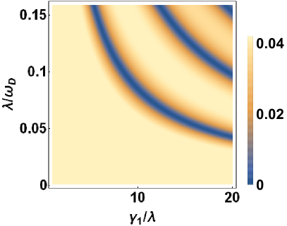
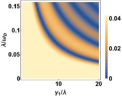
Figure 3: Top left Panel: Plot of the smallest Floquet bandgap for $H_{F}^{(1);s}$ as a function of $\lambda/(\hbar\omega_{D})$ and $\gamma_{1}/\lambda$. Top right panel: A similar plot corresponding to $H_{F}^{(1);c}$. Bottom Left (right) panel: Similar plot corresponding to the exact Floquet Hamiltonian for the discrete square pulse (continuous cosine drive) protocols. For all plots $\gamma=-0.35$ and $m=-0.08$. See text for details.

The plot of the smallest bandgap (the smallest difference in quasienergy between the lowest positive and highest negative quasienergy bands) of the Floquet Hamiltonian is shown in Fig. 3. The top panel shows the band gap as obtained using the expressions of $H_{F}$ from FPT as given in Eqs. 13, 14 and 17. The top left (right) panel shows the Floquet perturbation theory results for discrete square pulse (continuous cosine drive) protocols. These plots are compared to the exact results plotted in the respective bottom panels. The plots shows remarkable match in the high ($\hbar\omega_{D}\gg\gamma_{1}$) and intermediate frequency regime ($\hbar\omega_{D}\sim\gamma_{1}$) which clearly reflects the accuracy of FPT in this regime.

The plots in both the top and bottom panel indicate the presence of regimes with extremely small gaps in the Floquet spectrum as a function of $\gamma_{1}$ or $T$. These regimes appear around drive frequencies $T_{c}$ and amplitude $\gamma_{1c}$ which satisfy $\sqrt{2}\gamma_{1c}T_{c}/\hbar=2n\pi$ for the discrete protocol and along $\sqrt{2}\gamma_{1c}T_{c}/\hbar=\pi\alpha_{n}$ for the continuous protocol as shown in Fig. 3. This feature is easy to understand from the expressions of the first order Floquet Hamiltonians given in Eqs. 13 and 14; for these drive frequencies and amplitude both of these Hamiltonians reduce to

$$H_{F}^{\ast} = \frac{1}{2}\left[(a_{1}+a_{2})(\Gamma_{2}+\Gamma_{4})+ia_{5}(\Gamma_{2}\Gamma_{3}+\Gamma_{3}\Gamma_{4})\right],$$

which, as we shall see in Sec. IV.3, supports gapless bulk modes. Further, as shall be analyzed in details in Sec. IV.3, a relative sign change of the mass of the gapped edge modes occur at both the $x$ and one of the $y$ edges of the system as the system traverses through these nearly gapless points. The spectrum of the exact Floquet Hamiltonian, in contrast, retains a small gap across these points; we shall discuss this feature in details in Sec. IV.3.

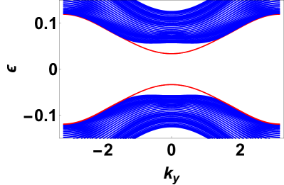
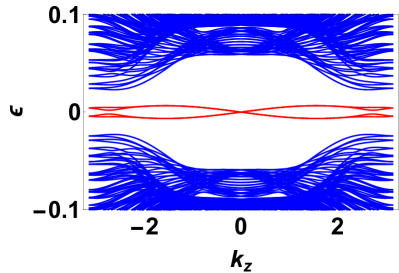
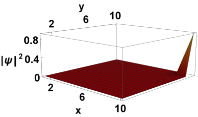
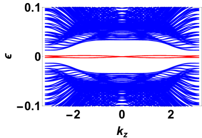
Figure 4: Top left panel: Plot of energy spectrum of the first order Floquet Hamiltonian $H_{F}^{(1);s}$ as a function of $k_{y}$ for $k_{z}=2$ with PBC along $z$ and $y$ and OBC along $x$ for $\sqrt{2}\gamma_{1}T/\hbar=\pi$. Top right panel: Surface bands of $H_{F}^{(1);s}$ plotted as a function of $k_{z}$ using OBC along $x$ and $y$. The red bands show Floquet hinge localized modes. Bottom left panel: Plot of $|\psi(x,y;k_{z}=1)|^{2}$ as a function of $x$ and $y$ for the Floquet hinge localized mode. Bottom right panel: Surface bands of $H_{F}^{(1);c}$ plotted as a function of $k_{z}$ using OBC along $x$ and $y$ for $\hbar\omega_{D}/\lambda=3.3$. For all plots $\gamma=-0.35$, $m=-0.08$.

For the square pulse protocol, the magnitude of the gap becomes smaller as the drive frequency is lowered from $T=2\pi\hbar/(\sqrt{2}\gamma_{1})$ as can be seen from the left panels of Fig. 3. This feature can be easily understood by noting that the terms in the Floquet Hamiltonian $H_{F}^{(1);s}$ which are to be added to $H_{F}^{\ast}$ to obtain a spectral gap have amplitudes $\sim 1/(\gamma_{1}T)$ and thus decrease rapidly with decreasing frequency. In contrast, for the continuous protocol, as shown in the right panel, the gap at higher frequencies is much more robust. This can be understood from the expression of $H_{F}^{(1);c}$ which indicates that the amplitude of the terms added to $H_{F}^{\ast}$ (Eq. LABEL:hfstar) for a finite spectral gap is proportional to $J_{0}(\sqrt{2}\gamma_{1}T/(\pi\hbar))$; their amplitude therefore decreases more slowly with decreasing frequency.

Thus we find that the Floquet Hamiltonians derived using FPT support near gapless regimes as a function of both $\gamma_{1}$ and $T$. We also note that the predictions based on first order FPT results are validated from numerical computations of the bulk spectrum gap of the exact Floquet Hamiltonians as shown in the bottom plots of Fig. 3. In the next subsections, we shall analyze the properties of these gapped and near-gapless phases for specific drive frequencies. We close this subsection by noting that the second order Magnus expansion can not explain these transitions as shown in the Appendix. The second order Floquet Hamiltonian obtained from the Magnus expansion yields Floquet phases with large gaps for both continuous and discrete protocols at all frequencies.

IV.2 Gapped phases of the first order Floquet Hamiltonian

In this section, we shall discuss the property of the gapped phases. For this purpose we shall use the square pulse protocol with a time period $T^{\prime}$ which satisfies $\sqrt{2}\gamma_{1}T^{\prime}/\hbar=\pi$. The reason for this choice is that the Floquet Hamiltonian $H_{F}^{(1);s}$ is particularly simple at this point making several aspects of the phase analytically tractable.

For $T=T^{\prime}$, the perturbative Floquet Hamiltonian can be written as

$$H_{F}^{(1);s}(T^{\prime}) = H_{F}^{\ast}-\frac{\sqrt{2}i\hbar}{\pi}\left((a_{1}-a_{2})\Gamma_{2}\Gamma_{4}\right.$$ (23)

$$\left.+(\Gamma_{2}+\Gamma_{4})(a_{3}\Gamma_{3}+a_{4}\Gamma_{1})+ia_{5}\Gamma_{3}\right).$$

The bulk spectrum of $H_{F}^{(1);s}(T^{\prime})$ is found to be gapped as can be seen from the top left panel of Fig. 4 where the energy spectrum is plotted as a function of $k_{y}$ for $k_{z}=2$ with open boundary condition (OBC) along $x$-direction and periodic boundary condition (PBC) along $z$ and $y$. This shows gapped surface states modes similar to the undriven case but does not show topologically protected zero energy surface modes.

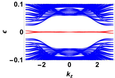
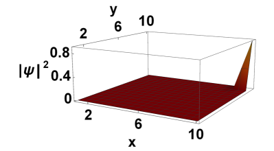
Figure 5: Left Panel: Surface bands of exact Floquet Hamiltonian for a square pulse protocol plotted as a function of $k_{z}$ using OBC along $x$ and $y$ with $\sqrt{2}\gamma_{1}T/\hbar=\pi$. Right Panel: Plot $|\psi(x,y;k_{z}=1)|^{2}$ as a function of $x$ and $y$ for the hinge mode. All parameters are same as those in Fig. 4

To check for the possibility of the topologically protected hinge modes, next we consider OBC along $x$ and $y$ directions in conjunction with PBC along $z$ and plot the band spectrum in the top right panel of Fig. 4 as a function of $k_{z}$. Interestingly, we find finite energy dispersive modes at the center of the bulk bands for $k_{z}\neq 0$. This is in contrast to the standard quadrupolar insulators which host gapless hinge modes. To identify the nature of this energy mode, we plot probability density of the corresponding eigenstate, $|\psi(x,y;k_{z})|^{2}$, in the $x-y$ plane for $k_{z}=1$ as shown in the bottom left panel Fig. 4. Clearly, the finite energy mode appears to be the hinge mode of driven Hamiltonian. Thus the Floquet Hamiltonian seems to support dispersing hinge modes at finite $k_{z}$. The energy of the hinge modes becomes zero at $k_{z}=0$ when $m$ is finite or at all values of $k_{z}$ which allow hinge modes when $m_{0}=0$. The bottom right panel of Fig. 4 shows the presence of hinge modes in the gapped phase of the Floquet Hamiltonian obtained using a continuous protocol for representative value of drive parameters. We find analogous dispersive hinge modes although the dispersion turns out to be flatter compared to its discrete protocol counterpart.

The hinge modes obtained from the analysis of $H_{F}^{(1);s}$ can be compared to the ones obtained from exact numerics for the same parameter value. The dispersion of these modes are shown in the left panel of Fig. 5 while the probability density $|\psi(x,y;k_{z}=1)|^{2}$ for the hinge states are plotted in the right panel of the figure. We find the presence of hinge modes in the spectrum of exact Floquet Hamiltonian for the square pulse protocol which is qualitatively consistent with the results obtained from $H_{F}^{(1);s}$. We note that the exact hinge modes display a much flatter dispersion compared to their analytic counterparts; moreover, they start to deviate from $E=0$ for $|k_{z}|\geq 2.6$ predicting absence of zero energy states beyond $-2.6\leq k_{z}\leq 2.6$ for the chosen set of parameters. The latter feature is also seen for $m_{0}=0$ where all modes with $|k_{z}|\leq 2.6$ correspond to $E=0$.

To understand such dispersing hinge modes, we first address the case with $m=0$. This is followed by a perturbative treatment for a small, non-zero value of $m$. The first-order Floquet Hamiltonian, given in Eq. (13) at this driving frequency is given, for $m=0$, by (Eq. 23)

$$H_{F}^{(1);s}(T^{\prime};\vec{k}) = \frac{1}{2}(2\gamma_{z}+\lambda\cos{k_{x}}+\lambda\cos{k_{y}})(\Gamma_{2}+\Gamma_{4})$$ (24)

$$-i\frac{\sqrt{2}\hbar}{\pi}\lambda\Big{[}(\Gamma_{2}+\Gamma_{4})(\sin{k_{x}}\Gamma_{3}+\sin{k_{y}}\Gamma_{1})$$

$$+(\cos{k_{x}}-\cos{k_{y}})\Gamma_{2}\Gamma_{4}\Big{]},$$

where we have used Eq. 1 for expressions of $a_{i}$ for $i=1..4$ and $\gamma_{z}$. The analysis of hinge modes can then be cast as a solution of the edge problem for $H_{F}^{(1);s}(T^{\prime};k_{x}=\pm k_{y},k_{z})$. For the sake of definiteness we choose $k_{x}=k_{y}=k$ here; along this line

$$H_{F}^{(1);s}(T^{\prime};k,k_{z})=\frac{1}{2}(2\gamma_{z}+2\lambda\cos{k})\Lambda_{1}-i\frac{\sqrt{2}\hbar}{\pi}\lambda\sin{k}\Lambda_{1}\Lambda_{2},$$ (25)

where $\Lambda_{1}=\Gamma_{2}+\Gamma_{4}$ and $\Lambda_{2}=\Gamma_{1}+\Gamma_{3}$. Eq. 25 corresponds to a 1D hopping Hamiltonian with its two ends at the two diagonally opposite corners of the original lattice (treating $k_{z}$ as a parameter). Thus the end modes of this Hamiltonian will correspond to any hinge localized mode of the original problem.

To find the end mode, we need a solution of

$$H_{F}^{(1);s}(T^{\prime};k=-i\partial_{\xi},k_{z})\phi(\xi) = E\phi(\xi),$$ (26)

with $\phi(\xi=0)=0$ where the edge is at $\xi=0$. Here we have chosen a semi-infinite line occupying $\xi>0$ and have used the identification $k=-i\partial_{\xi}$ with $\xi=\frac{1}{\sqrt{2}}(x+y)$. To this end, we consider the wavefunction $\phi_{\pm}$ given by

$$\phi_{\pm}(\xi) = e^{-\alpha\xi}e^{\pm i\beta\xi}\chi.$$ (27)

Substituting Eq. 27 in Eq. 26, we find

$$(\gamma_{z}+\lambda\cos{(i\alpha\pm\beta)})\Lambda_{1}\chi-i\frac{\sqrt{2}\hbar}{\pi}\lambda \sin{(i\alpha\pm\beta)}\Lambda_{1}\Lambda_{2}\chi$$

$$~{}~{}~{}~{}~{}~{}~{}~{}=E\chi.$$ (28)

Next, we try a solution of the form $\Lambda_{2}\chi=p\chi$ (where $p=\pm\sqrt{2}$ constitute the two doubly degenerate eigenvalues of $\Lambda_{2}$) and $E=0$. This leads to

$$\left((\gamma_{z}+\lambda\cos{(i\alpha\pm\beta)})-i\frac{\sqrt{2}\hbar}{\pi}\lambda\sin{(i\alpha\pm\beta)}p\right)\Lambda_{1}\chi=0.$$ (29)

For Eq. 29 to hold, we need to equate its real and imaginary parts to zero. This gives us the conditions

$$\gamma_{z}+\lambda\cosh{\alpha}\cos{\beta}=-\frac{\sqrt{2}\hbar}{\pi}\lambda p\sinh{\alpha}\cos{\beta},$$

$$\sinh{\alpha}\sin{\beta}=-\frac{\sqrt{2}\hbar}{\pi}p\cosh{\alpha}\sin{\beta},$$ (30)

which needs to be satisfied by $\alpha>0$ and $\beta$. If $\beta=\pi$, this therefore leads to the condition

$$\gamma_{z}\pm\lambda\cosh{\alpha}=\mp\frac{\sqrt{2}\hbar}{\pi}\lambda p\sinh{\alpha}.$$ (31)

This condition, however, is not satisfied for any $(k_{z},\alpha)$ pair corresponding to our chosen set of parameters. In contrast, for $\beta\neq 0,\pi/2,\pi$, we need

$$\tanh{\alpha} = -\frac{\sqrt{2}\hbar}{\pi}p,\quad\cos{\beta}=-\frac{\gamma_{z}}{\lambda}\cosh{\alpha}.$$ (32)

Also, we note that no solution exists for $\beta=\pi/2$ provided $\gamma_{z}\neq 0$.

For a localized solution at this edge, $\alpha$ should be positive; so $p$ should be chosen to be the negative eigenvalue of $\Lambda_{2}$, namely $-\sqrt{2}$ and $|\gamma_{z}/\lambda|<$ sech $\alpha$. This provides the allowed range of $k_{z}$ for zero-energy hinge modes for $m=0$. For our chosen set of parameter values, this second condition implies that our analysis does not hold for $|k_{z}|>2.6$. We note here that a similar analysis carried out for the diagonally opposite hinge (for which $\alpha<0$) would yield a similar solution but with $p$ chosen to be positive eigenvalues of $\Lambda_{2}$.

The analysis above indicates that there are two linearly independent solutions for $\chi_{1,2}$ given by

$$\psi_{1,2}(\xi) = \mathcal{N}e^{-\alpha\xi}\sin{(\beta\xi)}\chi_{1,2},$$ (33)

$$\chi_{1(2)} = \left(-\frac{i}{\sqrt{2}},+(-)\frac{i}{\sqrt{2}},0(1),1(0)\right)^{T}.$$

which satisfies $\psi(\xi=0)=0$. Here $\chi_{1,2}$ denotes the eignvectors of $\Lambda_{2}$ corresponding to $p=-\sqrt{2}$. We note that naively one may conclude the existence of two hinge modes per hinge from such a solution which contradicts exact numerics which yields one such state. It is to be stressed that our solution does not necessarily mean the existence of two such modes since the edge mode needs to respect $C_{4}^{z}$, $M_{y}$, $M_{x}$ and ${\mathcal{I}}$ symmetries. This may indeed lead to choice of a specific linear combination of the two solutions leading to the correct number of modes. However, a detailed analysis of this requires a solution constituting all four edge modes; we do not attempt it in this work.

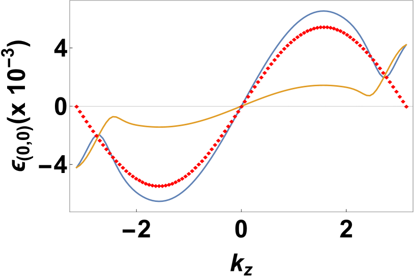
Figure 6: Plot of the hinge mode dispersion as a function of $k_{z}$ using analytical solution ($\mu_{1}$ from Eq. 35 with $m=-0.08$) [red squares], numerical solution of $H_{F}^{(1);s}$ using OBC along $x,y$ and PBC along $z$ (blue line) and $H_{F}$ obtained from exact numerics (yellow line). The analytical result shows near exact match with the numerical result obtained from $H_{F}^{(1);s}$ for small $k_{z}$. All parameters are same as those in bottom left panel of Fig. 5.

Instead, to understand the dispersion of the hinge modes in the presence of a finite $m_{0}$, we now switch to the case of non-zero $m_{0}$. We find that allowing the presence of a non-zero $a_{5}$ in Eq. 13 introduces an additional term in the $H_{F}^{(1);s}(T^{\prime};k,k_{z})$ (Eq. 25) given by

$$H_{m} = m_{0}\sin{k_{z}}\left(i(\Gamma_{2}\Gamma_{3}+\Gamma_{3}\Gamma_{4})-\frac{\sqrt{2}}{\pi}\Gamma_{3}\right).$$ (34)

Projecting this term in the space spanned by $\chi_{1,2}$ and diagonalizing, one obtains two eigenvalues and eigenvectors as

$$\mu_{a} = (-1)^{a}m_{0}\sin{k_{z}}(\pi+(-1)^{a}1)/\pi$$

$$\psi_{m,a} = \frac{1}{\sqrt{2}}\left(\psi_{1}+(-1)^{a+1}\psi_{2}\right)$$ (35)

where $a=1,2$. The mode which remain close to $E=0$ at small $m_{0}$ corresponds to $a=1$. As shown in Fig. 6, this mode shows remarkable match with the numerical spectrum obtained from $H_{F}^{(1);s}$ at $T=T^{\prime}$ for small $k_{z}$; however, it fails to reproduce the up turn of the spectrum at large $k_{z}$. It also shows qualitatively similar behavior to the corresponding exact hinge mode spectrum for small $k_{z}$ which produces a dispersing spectrum with much flatter dispersion. This prompts us to choose the linear combination $\psi\sim\psi_{1}+\psi_{2}$ as the hinge mode solution for $m_{0}=0$; the other mode corresponding to $a=2$ seems to be an artifact of treating a single hinge which we ignore. We also note that our analysis not only explains the dispersion of the hinge modes for finite $m_{0}$ but also predicts that for $m_{0}=0$, there are no zero energy hinge states for $k_{z}$ satisfying ${\rm sech}\alpha>|(\gamma_{z}/\lambda)|$ (which translates to $|k_{z}|>2.6$ for our chosen parameters). This matches with the result of exact numerics where the hinge modes for $m_{0}=0$ starts to deviate from zero energy beyond $|k_{z}|\sim 2.6$ for the chosen set of parameters.

IV.3 Gapless points in the first order Floquet spectrum

In this section, we shall analyze the Floquet Hamiltonian at the gapless point using the first order perturbative Hamiltonian which allows some analytic insight into the nature of these points. For the discrete square pulse protocol such points occur at $\sqrt{2}\,\gamma_{1}\,T/\hbar=2n\pi$ while for the continuous protocol, they occur at $\sqrt{2}\gamma_{1}T/\hbar=\pi\alpha_{n}$. For both these points, the first order perturbation theory yields $H=H_{F}^{\ast}$. In this section, we shall analyze the bulk and the surface properties of $H_{F}^{\ast}$.

IV.3.1 Bulk modes

We begin our analysis with the bulk modes of $H_{F}^{\ast}$ using PBC in all directions. This yields

$$\epsilon_{\pm,\pm}=\pm\frac{1}{\sqrt{2}}||a_{1}+a_{2}|\pm|a_{5}||.$$ (36)

It turns out that the spectrum contains zero energy curves which constitutes stacks of Weyl nodes for $k_{z}\neq 0,\pi$ and Dirac nodes for $k_{z}=0,\pi$. The former constitutes a crossing of two bands leading to Weyl nodes at the crossing points. At $k_{z}=0,\pi$, both the positive and negative quasienergy bands are two-fold degenerate; hence in this case, one has a crossing of all four bands leading to Dirac nodes.

The generic condition on the momenta $(k_{x},k_{y},k_{z})$ for these band crossings is given by

$$-\sqrt{1+m^{2}}\leq\mu(k_{x},k_{y})\leq\sqrt{1+m^{2}},$$ (37)

$$\cos k_{z}^{\pm}=\frac{\mu(k_{x},k_{y})}{1+m^{2}}\pm\frac{|m|}{1+m^{2}}\sqrt{1+m^{2}-\mu^{2}(k_{x},k_{y})},$$

where we have used Eqs. 36 and 1 and $\mu(k_{x},k_{y})=(2\gamma+\cos k_{x}+\cos k_{y})$. The band spectrum corresponding to Eq. 36, shown in Fig. 7, demonstrates these nodes for different values of $k_{z}$. Notice that for fixed $k_{z}$, the bulk gap closes in the $k_{x}-k_{y}$ plane along a single or multiple curves, giving rise to nodal lines/rings Weyl (for $k_{z}\neq 0,\pi$) or Dirac semimetals (for $k_{z}=0,\pi$) young_PRL15 . The shape of the lines/rings depends on the values of $k_{z},\gamma$ and $m$ and is determined by Eq. 37. We note that the Dirac line nodes on mirror-invariant planes $k_{z}=0$ and $k_{z}=\pi$ are protected by $M_{z}$, $I$ and $T_{0}$ symmetries which leads to the two-fold degeneracy of the bulk bands. For $k_{z}\neq 0,\pi$, these symmetries are broken; this leads to lifting of the degeneracies and a generic crossing between two non-degenerate bands leading to Weyl nodes.

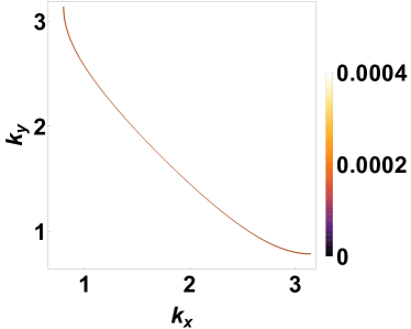
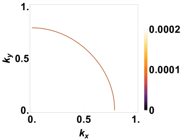
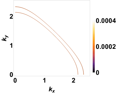
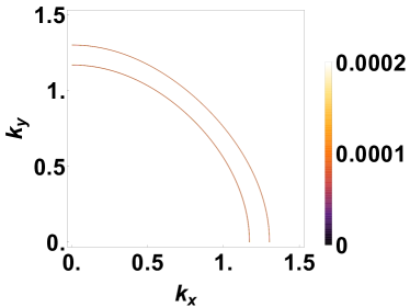
Figure 7: Contour plot of $\epsilon_{+,-}$ in the $k_{x}-k_{y}$ plane. Top left panel: For $k_{z}=0$, the two-fold degenerate conduction and valence bands meet along the arcs, giving rise to line node Dirac semimetals. Right panel: For $k_{z}=\pi$. Bottom left panel: For $k_{z}=1.25$ where two bands cross leading to line node Weyl semimetal. Right panel: For $k_{z}=2.25$. For all plots $\gamma=-0.35$, and $m=-0.08$.

As explained earlier at the closing of Sec. III, the gaps for the bulk Floquet mode of the exact Hamiltonian do not close. This can be seen by looking at the Floquet spectrum in Fig. 8. These plots are almost identical except for the presence of a tiny gap in the spectrum in the regions where the first order Floquet theory yields gapless Weyl or Dirac nodes. Thus the band crossings of the first order theory becomes avoided level crossings for the exact Floquet Hamiltonian. The effect of this reduction of the bulk Floquet gap on the hinge modes shall be discussed in Sec. V. For both Fig. 7 and 8, we have set the plot range so as to only highlight the contours along which the bulk band gap is the smallest.

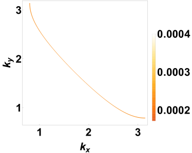
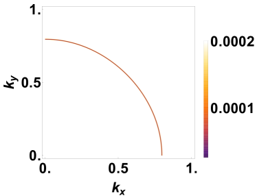
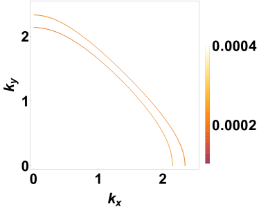
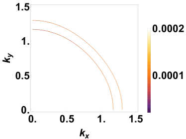
Figure 8: Contour plot of $\epsilon_{+,-}$ for the exact Floquet Hamiltonian in the $k_{x}-k_{y}$ plane for the square pulse protocol with $\sqrt{2}\gamma_{1}T/\hbar=2\pi$. All parameters are same as the corresponding panels in Fig. 7. Note that the gaps do not close exactly leading to an avoided level crossing.

IV.3.2 Surface and hinge modes

In this section, we shall analyze the surface and hinge modes around the drive frequencies at which the bulk spectrum gap for the first order Hamiltonian closes. Thus we shall be concerned with drive frequencies $\sqrt{2}\gamma_{1}T/\hbar=2n\pi+\delta$ for the discrete protocol and $\sqrt{2}\gamma_{1}T/\hbar=\pi\alpha_{n}+\delta$ for the continuous protocol, where $|\delta|\ll 2\pi$. For both these protocols, the effective Floquet Hamiltonian in this region, for $m=0$, reads

$$H_{\rm eff} = H_{F}^{\ast}+\delta c_{0}[(a_{1}-a_{2})(\Gamma_{4}-\Gamma_{2})+2(a_{3}\Gamma_{3}+a_{4}\Gamma_{1})],$$

where $c_{0}$ is a protocol dependent constant which takes values $c_{0s}=1/(4\pi)$ for the discrete protocol and $c_{0c}=J_{-1}(\alpha_{n})/\pi$ for the continuous protocol. The bulk modes corresponding to PBC are easily calculated to be

$$\epsilon_{\pm}=\pm\frac{1}{\sqrt{2}}\bigg{[}(a_{1}+a_{2})^{2}+4\delta^{2}c_{0}^{2}((a_{1}-a_{2})^{2}+2(a_{3}^{2}+a_{4}^{2}))\bigg{]}^{1/2},$$ (39)

which show a band touching at $\delta=0$ for $\vec{k}$ values which yields gapless modes.

In what follows we shall first analyze the surface modes of $H_{\rm eff}$ as a function of $\delta$. To this end, we use the continuum limit of this lattice Hamiltonian by expanding around the point $(k_{x},k_{y})=(0,0)$ and keeping terms till second order in the momenta. When dealing with the $x=0$ surface specifically, $k_{y}$ will remain a good quantum number, so that, we can neglect the negligible $k_{y}^{2}$ terms and write the Hamiltonian as a sum of two parts, viz

$$H(-i\partial/\partial x,k_{y},k_{z})=H^{I}+H^{II}.$$ (40)

Here $H^{I}$ carries the whole $x$ dependence and is given by

$$H^{I}= \frac{1}{2}(\gamma_{z}+\lambda)(\Gamma_{2}+\Gamma_{4})+\frac{\lambda}{4}\frac{\partial^{2}}{\partial x^{2}}(\Gamma_{2}+\Gamma_{4})$$

$$+\frac{\delta\lambda}{8\pi}\frac{\partial^{2}}{\partial x^{2}}(\Gamma_{4}-\Gamma_{2})-i\frac{\delta\lambda}{2\pi}\frac{\partial}{\partial x}\Gamma_{3},$$ (41)

while $H^{II}$, which carries the entire $k_{y}$ dependence, can be written as

$$H^{II}=\frac{1}{2}(\gamma_{z}+\lambda)(\Gamma_{2}+\Gamma_{4})+\frac{\delta\lambda}{2\pi}k_{y}\Gamma_{1}.$$ (42)

Here and in rest of the section, we choose to work with $c_{os}$ for clarity. The form of Eq. LABEL:effham guarantees that this does not lead to a loss of generality.

For a surface localized state, we choose as our ansatz $\psi_{k_{y},k_{z}}(x)\sim\exp{(\alpha x)}e^{i(k_{y}y+k_{z}z)}\sin{(\beta x)}\Phi$, satisfying the boundary condition $\psi(x=0)=0$. We note that this corresponds to a choice of a semi-infinite system along $x$ occupying $x>0$ for $\alpha<0$. Plugging in this ansatz in $H^{I}\psi_{k_{y},k_{z}}(x)$, one gets

$$H^{I}\psi_{k_{y},k_{z}}(x) = \sin{(\beta x)}\bigg{[}\bigg{(}\frac{1}{2}(\gamma_{z}+\lambda)+\frac{\lambda}{4}(\alpha^{2}-\beta^{2})\bigg{)}(\Gamma_{2}+\Gamma_{4})+\frac{\delta\lambda}{8\pi}(\alpha^{2}-\beta^{2})(\Gamma_{4}-\Gamma_{2})-i\frac{\delta\lambda}{2\pi}\alpha\Gamma_{3}\bigg{]}\Phi$$ (43)

$$+\cos{(\beta x)}\bigg{[}\frac{\lambda}{2}\alpha\beta(\Gamma_{2}+\Gamma_{4})+\frac{\delta\lambda}{4\pi}\alpha\beta(\Gamma_{4}-\Gamma_{2})-i\frac{\delta\lambda}{2\pi}\beta\Gamma_{3}\bigg{]}\Phi.$$

For $\psi_{k_{y},k_{z}}(x)$ to be an eigenfunction of $H^{I}$, we need two conditions on $\Phi$. First, the coefficient of the $\cos\beta x$ term in Eq. 43 must vanish. Second, $\Phi$ should be an eigenvector of the matrix appearing in the coefficient of $\sin\beta x$. The first condition implies that $\Phi$ should satisfy

$$\left[\alpha(\Gamma_{2}+\Gamma_{4})+\alpha b/2(\Gamma_{4}-\Gamma_{2})-ib\Gamma_{3}\right]\Phi=0,$$ (44)

where $b=\delta/\pi$. The value of $\alpha$ satisfying this and the localization condition which necessitates a negative value of $\alpha$ is $\alpha=-\sqrt{\frac{2b^{2}}{4+b^{2}}}$. This yields two degenerate eigenvectors $\Phi_{1,2}$. Projecting the $\Gamma$ matrices in this null space spanned by $\Phi_{1,2}$, one finds that the coefficient of the $\sin\beta x$ term in this space is proportional to $\sigma_{x}$. Thus, to satisfy the second condition, the basis vectors of this nullspace should be chosen as $\chi_{\pm}=\frac{1}{\sqrt{2}}\begin{pmatrix}1\\ \pm\text{sgn}(b)\end{pmatrix}$. where ${\rm sgn}(b)$ denotes the sign of $b$. We note that the choice of these eigenvectors need to be carefully done to maintain the same definition of $\sigma_{x}$ for $b>0$ and $b<0$. Projecting $H^{II}$ in this space gives the surface Hamiltonian at this surface to be

$$H^{\delta>0}_{x=0}=-\frac{\lambda|b|}{2}k_{y}\sigma_{y}-(\gamma_{z}+\lambda)\frac{b}{\sqrt{2(4+b^{2})}}\sigma_{z}.$$ (45)

Thus the mass term changes sign with $b$. An exactly similar analysis can be carried out for other edges.

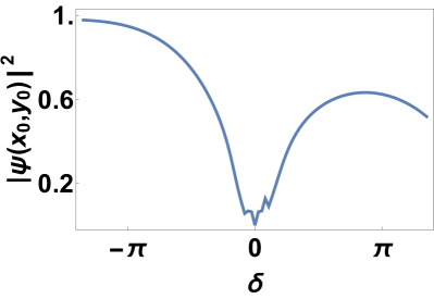
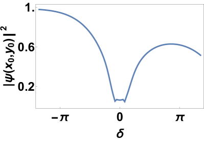
Figure 9: Left Panel: Plot of the probability density of the hinge mode, $|\psi(x_{0},y_{0};k_{z}=1)|^{2}$, as a function of $\delta$ as obtained from first order perturbative Floquet Hamiltonian for a square pulse protocol. Right panel: Same as the left panel but using exact Floquet Hamiltonian. For all plots, $\gamma_{1}/\lambda=20.0$, $\gamma=-0.35$, and $m=-0.08$. The chosen hinge corresponds to $x_{0}=y_{0}=1$ and we note that the behavior remains the same if we focus on any one of the four hinges.

Next, we study the hinge modes for small $\delta$. To this end we plot the probability density $|\psi(x=x_{0},y=y_{0})|^{2}$ (where $x_{0}=y_{0}=1$ is one of the hinges) as a function of $\delta$. We find that the hinge modes leak into the bulk around $\delta=0$ where the gap in the first order Floquet Hamiltonian closes as can be seen from Fig. 9. We also find that the probability density $|\psi(x_{0}=1,y_{0}=1;k_{z}=1)|^{2}$ for the hinge modes dips to a value close to zero for the exact Floquet spectrum where the gap remains finite at all drive frequencies. Thus we find that the hinge modes of $H_{F}$ leak significantly into the bulk at specific drive frequencies for which the first order Floquet Hamiltonian vanish. We shall explore the dynamical consequence of such hybridization in the next section.

V Dynamics of the hinge modes

In this section, we study the dynamics of hinge modes for two representative drive frequencies for the square pulse protocol. The first corresponds to $\sqrt{2}\gamma_{1}T/\hbar=\pi,3\pi$ where the Floquet Hamiltonian has large gap while the second corresponds to $\sqrt{2}\gamma_{1}T/\hbar=2\pi$ where they are almost gapless. In what follows, we shall study the time evolution of the wavefunction hinge modes localized at each hinge of the sample. The probability amplitude of the driven wavefunction can be probed experimentally as we discuss below; hence it serves as a diagnostic tool of the Floquet phases outlined in the previous sections.

For a fixed $k_{z}$, $H_{0}$ (Eq. 1) supports four degenerate states at zero energy when Eq. 4 is satisfied. With appropriate linear combination of these states, we obtain four zero energy states localized at the four hinges of the sample. We start with one of these hinge modes whose wavefunction is given by $|\psi(0)\rangle$ as the initial state and study its evolution under the square pulse protocol. We consider a system with $L=10$ units cells along $x$ and $y$ and numerically compute the exact stroboscopic time-evolution operator given by Eq. 18 using OBC along $x$ and $y$ and PBC along $z$. We obtain $|\psi(nT)\rangle=U^{n}(T,0)|\psi(0)\rangle$. For each of the four hinge unit cells, chosen to be at $(x,y)=(1,1)$, $(1,L)$, $(L,1)$ and $(L,L)$, we designate the initial state $|\psi(0)\rangle$ which is localized in the $\alpha^{\rm th}$ hinge of the system as $|\psi^{\alpha}(0)\rangle$.

Next, we define column vectors $|\phi_{i}^{\beta}\rangle$ having weight on the $i^{\rm th}$ site ($i=1,2,3,4$) of a unit cell $\beta$ in the $x-y$ plane. We then probe the evolution of the quantity,

$$\Phi^{\beta}(nT) = \sum_{i=1}^{4}|\langle\phi_{i}^{\beta}|\psi(nT)\rangle|^{2}=\sum_{i=1}^{4}\Phi_{i}^{\beta}(nT).$$ (46)

as a function of $n$. The value of this quantity gives an estimate of the weight of the state in any given unit cell $\beta$. Our definition ensures that $\Phi^{\beta}(0)\sim\delta_{\alpha\beta}$ is localized within the sites of the unit cell in the $\alpha^{\rm th}$ hinge. We note that $\Phi_{i}^{\beta}(nT)$, being proportional to the local electronic density of states, can be directly probed experimentally through scanning tunneling microscopic (STM) measurements.

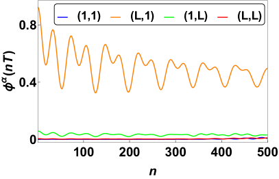
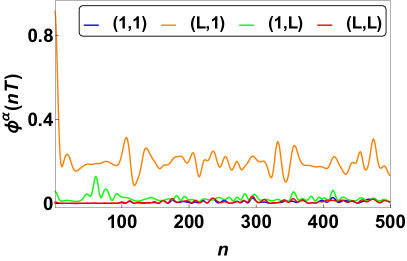
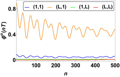
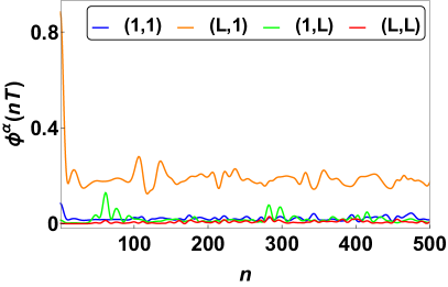
Figure 10: Top Panels: Stroboscopic evolution of $\Phi^{\alpha}(nT)$ where $\alpha$ denotes the unit cell at each of the hinges $(1,1)$, $(1,L)$, $(L,1)$ and $(L,L)$ for $m=0$ as a function of $n$ for $\sqrt{2}\gamma_{1}T/\hbar=\pi$ (left panel) and $\sqrt{2}\gamma_{1}T/\hbar=3\pi$ (right panel). Bottom panels: Same as corresponding top panels but with $m=-0.08$. For all plots $\gamma=-0.35$, $k_{z}=0.5$, and $\gamma_{1}/\lambda=20$.

Fig. 10 illustrates the evolution of spectral weight of the hinge state initially localized at site $(L,1)$ for $\sqrt{2}\gamma_{1}T=\pi,3\pi$ for both $m=0$ and a non-zero $m=-0.08$. For both values of $m$ we find qualitatively similar behavior; $\Phi^{\beta}(nT)$ assume appreciable non-zero value for $\beta\sim\alpha$ for all $n$. This indicates that the state at any stroboscopic time $t=nT$ remains mostly localized around the hinge at which it had an initial large overlap. For $\sqrt{2}\gamma_{1}T/\hbar=3\pi$, the state delocalizes to a greater extent which is due to the presence of a smaller bulk Floquet gap. This can be further understood from the spatial contour of the hinge state shown in Fig. 11 after representative number ($n$) of drive periods. We find that the weight of the hinge state always remains localized to the hinge where it was initially localized; this behavior is consistent with having a gapped Floquet spectrum at the bulk.

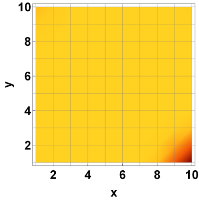
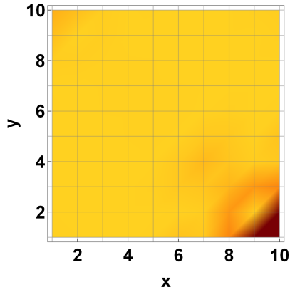
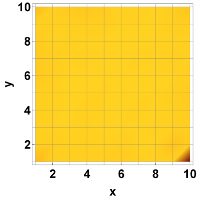
Figure 11: Plot of the spatial profile of $\Phi^{\beta}(nT)$ with $\sqrt{2}\gamma_{1}T/\hbar=\pi$ for a system with $L=10$ unit cells each along $x$ and $y$ in the $x-y$ plane. The top panels correspond to $n=20$ (left) and $32$ (right) while the bottom panels correspond to $n=126$ (left) and $3267$ (right). All other parameters are same as top panels of Fig. 10.

The dynamical behavior of the hinge modes can be further understood by examining the overlap of our initial state with the Floquet eigenstates, $P_{F}^{n}=|\langle\xi_{F}^{n}|\psi^{\alpha}(0)\rangle|^{2}$ as shown in the top left panel of Fig. 12. The Floquet eigenstates having appreciable overlap with the initial states are encircled in red; these include the four zero energy states (ZES). These coefficients do not change with time and thus provide a base average value about which the fluctuation occurs. This value is larger for higher drive frequency where the gap is larger. The analysis of the Fourier modes shown in the right panels of Fig. 12 yields constituent frequencies of these fluctuations. These turn out to be consistent with the difference in quasienergy values on which the initial state has substantial projections. We note that for $\sqrt{2}\gamma_{1}T/\hbar=3\pi$, there is a rapid dissipation of the state in the bulk. The difference in this case stems from the fact that the Floquet ZES are separated from the bulk by a reduced energy gap, resulting in a faster decay. The corresponding Fourier weights of the mode, $A(\omega)$, shown in the bottom right panel of Fig. 12, indicates the presence of multiple Fourier modes with small overlap due to which the dynamics appears incoherent. We have checked that this behavior remains qualitatively similar even when a small finite $m$ is switched on.

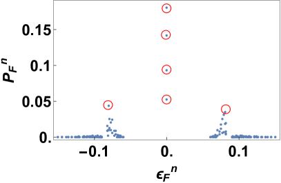
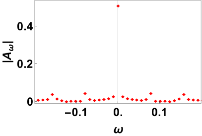
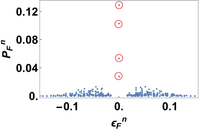
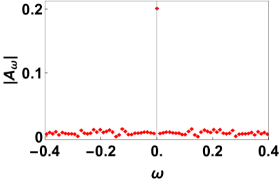
Figure 12: Top left panel: Plot of overlap probability $P_{F}^{n}=|\langle\xi_{F}^{n}|\psi^{\alpha}(0)\rangle|^{2}$ of the initial state $|\psi^{\alpha}(0)\rangle$ localized at the hinge $\alpha$ at $(L,1)$ with the Floquet eigenstates $|\xi_{F}^{n}\rangle$ for $\sqrt{2}\gamma_{1}T/\hbar=\pi$ and $m=0$. Top right panel: Fourier modes of the dynamics for $\sqrt{2}\gamma_{1}T/\hbar=\pi$ and $m=0$. Bottom panels: Same as corresponding top panels but for $\sqrt{2}\gamma_{1}T/\hbar=3\pi$. All other parameters are same as in Fig. 10.

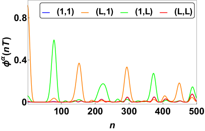
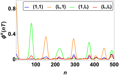
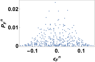
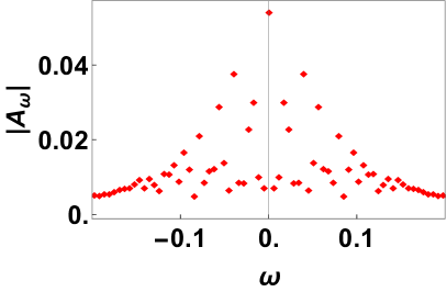
Figure 13: Top panels: Stroboscopic evolution of $\Phi^{\alpha}(nT)$ where $\alpha$ denotes the unit cell at each of the hinges $(1,1)$, $(1,L)$, $(L,1)$ and $(L,L)$ as a function of $n$ for $\sqrt{2}\gamma_{1}T/\hbar=2\pi$ with $m=0$ (left panel) and $m=-0.08$ (right panel). Bottom panels: Plot of the overlap $P_{F}^{n}$ (left panel) and the Fourier modes $A(\omega)$ (right panel). Both plots correspond to $\sqrt{2}\gamma_{1}T/\hbar=2\pi$ and $m=0$. All other parameters are same as in Fig. 10.

For $\sqrt{2}\gamma_{1}T/\hbar=2\pi$, where the bulk Floquet spectrum is almost gapless, the dynamics of the hinge mode is qualitatively different, as shown in Fig. 13. We find that the hinge mode shows almost coherent transport between the diagonally opposite hinges as shown in the top panels of Fig. 13. The weight of the state starts being localized at the unit cell of hinge $(L,1)$ and reaches the hinge $(1,L)$ after $n\sim 80$ cycles; after $n\sim 160$ cycles of the drive, the weight of the state again becomes localized at the hinge where its initial weight was large. We note that this does not necessarily mean that the wavefunction of the driven hinge state after $n\sim 160$ cycles exhibits large overlap with the initial wavefunction; there exists significant difference in the distribution of weights of these wavefunctions within the hinge unit cell. As shown in the bottom panels of Fig. 13, the spectral weight $P_{F}^{n}$ has a large overlap with several bulk Floquet modes and has finite weight in several Fourier modes. This also is in sharp contrast to that found for $\sqrt{2}\gamma_{1}T/\hbar=\pi$ where the bulk Floquet gap is large; for the latter case, the wavefunction of the hinge mode has significant overlap with only a few Floquet modes.

The difference in dynamics of the hinge mode for $\sqrt{2}\gamma_{1}T/\hbar=2\pi$ and $\sqrt{2}\gamma_{1}T/\hbar=\pi$ can be further understood from the spatial profile of $\Phi^{\beta}(nT)$ for representative values of $n$ as shown in Fig. 14. We find that at intermediate times $0<n<80$, the amplitude of the driven state is spread out in the bulk as can be seen from the top right panel of Fig. 14. In contrast, for $n\simeq 80p$, where $p$ is integer, they are localized in one of the two diagonally opposite hinges with spread along the respective surfaces. All of these features indicate qualitatively different hinge mode dynamics for $\sqrt{2}\gamma_{1}T/\hbar=2\pi$.

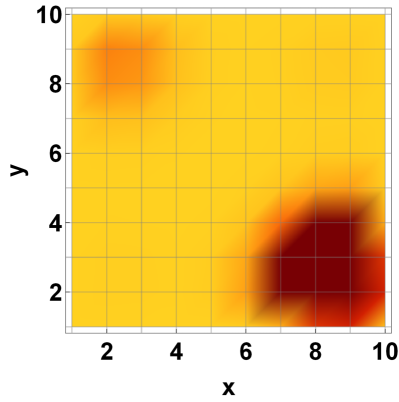
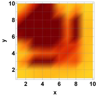
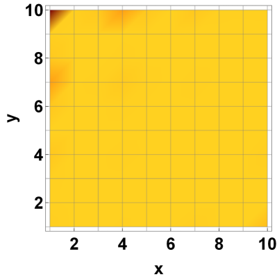
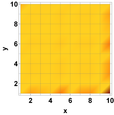
Figure 14: Plot of the spatial profile of $\Phi_{i}^{\beta}(nT)$ with $\sqrt{2}\gamma_{1}T/\hbar=2\pi$ for a system with $L=10$ unit cells each along $x$ and $y$ in the $x-y$ plane: (a) $n=20$, (b) n=$52$, (c) $n=80$, and (d) n=$153$. All other parameters are same as in Fig. 10.

To obtain a qualitative analytic understanding of the behavior of these hinge modes, we note that, in contrast to their counterparts for $\sqrt{2}\gamma_{1}T/\hbar=\pi,3\pi$, several bulk Floquet modes have high overlap with the initial state representing the hinge mode. Thus the state representing the driven hinge mode can be written as

$$|\psi(nT)\rangle = \sum_{m}c_{\alpha m}e^{-iE_{m}^{F}nT}|m\rangle,$$ (47)

where $c_{\alpha m}=\langle m|\psi_{\alpha}(0)\rangle$, $|m\rangle$ denote the bulk Floquet states, and $E_{F}^{m}$ are their quasienergies. For having analytic insight into the problem, we now assume the bulk Floquet modes are almost similar to the ones with periodic boundary condition; in this, one can replace $|m\rangle$ with $|k\rangle$ and $E_{m}^{F}$ with $E_{a}^{F}(\vec{k})$. There are four such eigenvalues for each $\vec{k}$ as given by Eq. 36; we label these with the index $a$ assuming values $1,2,3,4$. The sum over $m$ can then be replaced by an integral over $k$ and a sum over the index $a$ and we obtain

$$\psi(x,y;nT) = \sum_{a=1,4}\int\frac{d^{2}k}{(2\pi)^{2}}c^{a}_{\alpha}(\vec{k})e^{i(\vec{k}\cdot\vec{r}-E_{a}^{F}({\vec{k}})nT)}$$

$$= \sum_{a=1,4}\int\frac{d^{2}k}{(2\pi)^{2}}c^{a}_{\alpha}(\vec{k})e^{in\Xi^{a}(x,y,:\vec{k})},$$

$$\Xi^{a}(x,y;{\vec{k}}) = (k_{x}x+k_{y}y)/n-E_{a}^{F}(\vec{k})T,$$ (48)

where ${\vec{r}}=(x,y)$ and $a$ denotes index for eigenvalues (Eq. 36) and the corresponding eigenvectors. For large $n$, thus the contribution to $\psi(x,y;n)$ comes from coordinates which satisfy $\partial_{k_{x}}\Xi^{a}(x,y;\vec{k})=\partial_{k_{y}}\Xi^{a}(x,y;\vec{k})=0$. Using Eqs. 36, we find that these are given by

$$\frac{x}{n} = \pm\frac{\lambda T}{\sqrt{2}}\sin k_{x}^{0},\quad\frac{y}{n}=\pm\frac{\lambda T}{\sqrt{2}}\sin k_{y}^{0}.$$ (49)

We now use this to find the shortest number of drive cycles at which the state reaches the diagonally opposite hinge, we seek a solution of Eq. 49 for $x=y=L$ and smallest possible $n_{c}>0$. This yields $k_{x}^{0}=k_{y}^{0}=\pm\pi/2$ so that $n_{c}=L\gamma_{1}/(\lambda\pi)$. For $L=10$ and $\gamma_{1}=20\lambda$, this yields $n_{c}=64$ which is close to the numerical value of $n_{c}\sim 80$ (Fig. 14). This analytical result can be validated by plotting $n_{c}$, obtained from exact numerics, as a function $L$ and $\gamma_{1}$, as shown in Fig. 15. We find that in accordance with the analytic prediction, $n_{c}$ varies linearly with both $L$ and $\gamma_{1}$. For $L=10$, the slope of the plot of $n_{c}$ as a function of $\gamma_{1}$ is found to be $3.9$ while the theoretical prediction turns out to be $L/(\lambda\pi)\simeq 3.2$. Similarly, for $\gamma_{1}/\lambda=20$, the slope of the best fit for $n_{c}(L)$ is found to be $7.4$ while the theoretical prediction is $\gamma_{1}/(\lambda\pi)=6.4$. This difference is partly due to a finite $n_{c}$ which induces additional corrections to the saddle point value. Thus the time period between revivals of the hinge mode shown in the top left panel of Fig. 13 can be qualitatively understood using this approximate saddle point analysis; however, one needs to go beyond this simple analysis to obtain more accurate value of $n_{c}$.

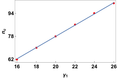
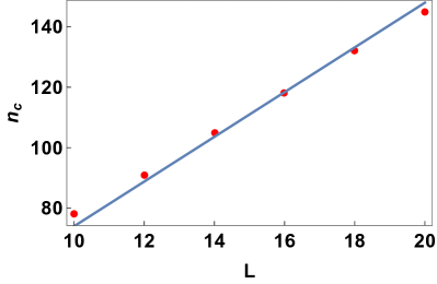
Figure 15: Plot of $n_{c}$ as a function of $\gamma_{1}$, with $\lambda=1$ for $L=10$ (left panel) and as a function of $L$ for $\gamma_{1}/\lambda=20$ (right panel). Both the plots indicate linear dependence of $n_{c}$ in accordance with the prediction of the saddle point analysis. All other parameters are same as in Fig. 10. See text for more details.

VI Discussion

In this work, we have studied the Floquet dynamics of hinge modes of second-order topological material modeled by free fermions hopping on a cubic lattice. The equilibrium phase diagram of the model shows topological transitions between gapped quadrupolar phase supporting zero energy hinge modes and gapless Weyl semimetals phase.

Upon driving the model by varying one of its parameter periodically with time, we find the existence of special drive frequencies at which the bulk gap for the Floquet quasispectrum almost vanishes. Such frequencies exists for both discrete square pulse and continuous cosine drive protocols. Our work shows that this effect can be analytically understood by computing the perturbative Floquet Hamiltonian of the system using FPT. In the large drive amplitude region, where FPT is expected to be accurate, a drive at these frequencies leads to vanishing bulk gap for the first order perturbative Floquet Hamiltonian. This happens at $\sqrt{2}\gamma_{1}T/\hbar=2n\pi$ for the discrete square protocol and $\sqrt{2}\gamma_{1}T/\hbar=\pi\alpha_{n}$ for the continuous cosine protocol. Thus the bulk gap becomes small since it can only originate from higher order terms in $H_{F}$; in the high drive amplitude regime, such terms are expected to be small. Thus the Floquet spectrum shows lines where the bulk quasienergy gap is small. We note that this reduction of the gap is not captured by the Floquet Hamiltonian obtained using second order Magnus expansion.

Our numerical analysis of the Floquet Hamiltonian can be extended to other protocols. An obvious extension may occur when the fermions are subjected to a periodically time-dependent vector potential arising from the presence of incident radiation. However, in this case, all terms of the Fermion Hamiltonian (Eq. 1) shall become time dependent. This makes the problem difficult to address using analytic Floquet perturbation theory. Another possibility is to use a protocol involving periodic kicks. In this case, one can extend our formalism in a straightforward manner and obtain results which are qualitatively similar to the square pulse protocol provided the drive parameters are chosen appropriately.

Away from these special points, where the bulk gap is large, our analysis finds Floquet hinge modes in the Floquet spectrum. We provide an analytic expression for these Floquet hinge modes for the discrete protocol with $\sqrt{2}\gamma_{1}T/\hbar=\pi$; we find that the analytical results agree qualitatively to exact numerics. In contrast to their equilibrium counterpart, these hinge modes have $k_{z}$ dependent dispersion as confirmed from both the first order analytic Floquet Hamiltonian and exact numerics. The dispersion of the hinge modes turns out to be flatter for continuous drive protocols; also the analysis based on first order Floquet Hamiltonian predicts stronger dispersion compared to that obtained using exact numerics. In contrast, near the special drive frequencies where the gap is small, the hinge modes leak into the bulk; they become almost indistinguishable from the bulk when the drive frequency matches these special frequencies.

The presence of the small Floquet quasienergy gap manifests in the dynamics of the hinge modes. To study such dynamics we start with an initial zero energy eigenstate of the equilibrium Hamiltonian $H_{0}$ which is localized at one of the hinge. We then study its dynamics by driving the system with two representative frequencies. One of these corresponds to the case where the bulk Floquet Hamiltonian is gapped. For the square pulse protocol, we choose $\sqrt{2}\gamma_{1}T/\hbar=\pi$. In this case we find that the hinge mode remains localized in the vicinity of its original position. In contrast, for systems driven with a frequency which satisfies $\sqrt{2}\gamma_{1}T/\hbar=2\pi$, the hinge mode propagates in the bulk and displays wavefront like propagation between diagonally opposite hinge. This becomes apparent by computing the spatially resolved probability of the driven wavefunction given by $\Phi^{\alpha}(nT)$. We find that $\Phi^{\alpha}(nT)$ shows distinct revivals; their time dependence represents motion of hinge modes between diagonally opposite hinges of the sample. Our analysis shows that the period of such a motion can be analytically understood within a saddle point analysis of the driven wavefunction.

The experimental verification of our theory can be achieved via STM measurements which track the local density of states for electrons within an unit cell. For an initial zero energy state localized at one of the hinge, the time variation of the local density of state will clearly depend on $\Phi^{\alpha}$. Our prediction is that starting from a hinge state localized at $(L,1)$, the dynamics with $\sqrt{2}\gamma_{1}T/\hbar=\pi$ will not show significant variation of $\Phi^{\alpha^{\prime}}(nT)$ for $\alpha^{\prime}$ corresponding to the diagonally opposite hinge $(1,L)$. In contrast $\Phi^{\alpha^{\prime}}(nT)$ will show periodic variations for $\sqrt{2}\gamma_{1}T/\hbar=2\pi$ with a period of $n_{c}$.

In conclusion, we have studied the Floquet spectrum and the hinge mode dynamics of driven second-order topological Weyl semimetals modeled by free fermions hopping on a cubic lattice. Our analysis reveals specific drive frequencies at which the bulk Floquet modes become nearly gapless. We also find that the dynamics of the hinge modes for such a Floquet Hamiltonian depend crucially on the proximity to these special frequencies; they remain localized close to their initial position away from these frequencies and propagates coherently between diagonally analogous hinges close to them. We suggest that the qualitative difference in such dynamics would be reflected in LDOS of fermions and shall therefore be measurable via STM measurements.

Appendix A Magnus expansion

In the appendix, we consider the Floquet Hamiltonian derived by the standard Magnus expansion method. The first-order correction in the Magnus expansion of the Floquet hamiltonian is given by

$$H_{{\rm mag}}^{(1)}=\frac{1}{T}\int_{0}^{T}dt_{1}H(t_{1}),$$ (50)

where $H(t_{i})=H_{0}+H^{\prime}(t_{i})$. Since for both discrete and continuous driving, we are using protocols which average out to zero over a complete cycle, therefore $H_{{\rm mag}}^{(1);s}=H_{{\rm mag}}^{(1);c}=H_{av}=H_{0}$. We note that this is equivalent to the results obtained from FPT in the limit $\gamma_{1}T\to 0$.

The second-order correction in the Magnus expansion is given by the expression

$$H_{{\rm mag}}^{(2)}=\frac{1}{2i\hbar T}\int_{0}^{T}\int_{0}^{t_{1}}dt_{1}dt_{2}[H(t_{1}),H(t_{2})].$$ (51)

For our chosen continuous drive protocol, $H(t)=H(T-t)$. It can be shown that for drives satisfying this symmetry condition, $H_{{\rm mag}}^{(2),c}=0$. Thus, till second order, the spectrum of $H_{{\rm mag}}^{c}$ is equivalent to that of $H_{av}$ which doesn’t exhibit a gap closing.

For the square pulse protocol, however, the second-order contribution is non-trivial and can be calculated as follows.

$$H_{{\rm mag}}^{(2),s}=\frac{1}{2i\hbar T}\int_{0}^{T}\int_{0}^{t_{1}}dt_{1}dt_{2}\left([H^{\prime}(t_{1}),H_{0}]+[H_{0},H^{\prime}(t_{2})]\right).$$ (52)

Evaluation of these commutators is straightforward, and one can show that

$$H_{{\rm mag}}^{(2),s}=\frac{\gamma_{1}T}{2i\hbar}((a_{1}-a_{2})\Gamma_{2}\Gamma_{4}+(\Gamma_{2}+\Gamma_{4}) (a_{3}\Gamma_{3}+a_{4}\Gamma_{1})$$

$$+ia_{5}\Gamma_{3}).$$ (53)

The eigenvalues of $H_{{\rm mag}}^{(1),s}+H_{{\rm mag}}^{(2),s}$ are

$$E^{{\rm mag},s}_{\pm,\pm}=\pm\frac{1}{2}\Big{(}4\sum_{i=1}^{5}a_{i}^{2} +((a_{1}-a_{2})^{2}+2(a_{3}^{2}+a_{4}^{2})+a_{5}^{2})(\gamma_{1}T/\hbar)^{2}$$

$$\pm 2|a_{5}|\sqrt{16(a_{1}^{2}+a_{4}^{2})+4(2a_{1}(a_{1}-a_{2})+3a_{4}^{2})(\gamma_{1}T/\hbar)^{2}+((a_{1}-a_{2})^{2}+2a_{4}^{2})(\gamma_{1}T/\hbar)^{4}}\Big{)}^{1/2}.$$ (54)

However, this neither reproduces the band closing nor even the substantial reduction in the bandgap at the special points $\sqrt{2}\gamma_{1}T/\hbar=2n\pi$, which we had obtained from first order FPT and exact numerics respectively.

References

- (1) M. Z. Hasan and C. L. Kane, Rev. Mod. Phys. 82, 3045 (2010); X.-L. Qi and S.-C. Zhang, Rev. Mod. Phys. 83, 1057 (2011).
- (2) C. L. Kane and E. J. Mele, Phys. Rev. Lett. 95, 226801 (2005); ibid, Phys. Rev. Lett. 95, 146802 (2006).
- (3) L. Fu, C. L. Kane, and E. J. Mele, Phys. Rev. Lett. 98, 106803 (2007); R. Roy, Phys. Rev. B 79, 195322 (2009); J. E. Moore and L. Balents, Phys. Rev. B 75, 121306 (2007).
- (4) S. Murakami, New Journal of Physics 9, 356 (2007); S. Murakami, S. Iso, Y. Avishai, M. Onoda, and N. Nagaosa, Phys. Rev. B 76, 205304 (2007).
- (5) X. Wan, A. M. Turner, A. Vishwanath, and S. Y. Savrasov, Phys. Rev. B 83, 205101 (2011); A. A. Burkov and L. Balents, Phys. Rev. Lett. 107, 127205 (2011).
- (6) N. P. Armitage, E. J. Mele, and A. Vishwanath, Rev. Mod. Phys. 90, 015001 (2018).
- (7) W.A. Benalcazar, B.A. Bernevig and T.L. Hughes, Science 357 6346 (2017).
- (8) W.A. Benalcazar, B.A. Bernevig and T.L. Hughes, Phys. Rev B 96, 245115 (2017).
- (9) F. Schindler, A.M. Cook, M.G. Verniory, Z. Wang, S.S.P. Parkin, B.A. Bernevig and T. Neupert, Sci. Adv. 4, eaat0346 (2018).
- (10) Z. Song, Z. Fang and C. Fang, Phys. Rev. Lett. 119 246402 (2017).
- (11) J. Langbehn, Y. Peng, L. Trifunovic, F.V. Oppen and P.W. Brouwer, Phys. Rev. Lett. 119 246401 (2017).
- (12) M.J. Park, Y. Kim, G.Y. Cho and S Lee, Phys Rev Lett 123, 216803 (2019).
- (13) RX Zhang, YT Hsu and S. Das Sarma, Phys Rev B 102, 094503 (2020).
- (14) H. Xue, Y. Yang, F. Gao, Y. Chong and B. Zhang, Nature Mat 18, 108-112 (2019).
- (15) M. Geier, L. Trifunovic, M. Hoskam, P.W. Brouwer, Phys Rev B 97, 205135 (2018).
- (16) Y. You, T. Devakul, F.J. Burnell and T. Neupert, Phys Rev B 98 235102 (2018).
- (17) T. Liu, J.J. He and F. Nori, Phys Rev B 98 245413 (2018).
- (18) Q. Wang, C.C. Liu, Y.M. Lu and F. Zhang, Phys Rev Lett 121 186801 (2018).
- (19) X. Zhu, Phys Rev B 97 205134 (2018).
- (20) K. Laubscher, D. Loss and J. Klinovaja, Phys Rev Research 1 032017(R) (2019).
- (21) Z. Yan, Phys Rev Lett 123 177001 (2019).
- (22) M. Kheirkhah, Y. Nagai, C. Chen and F. Marsiglio, Phys Rev B 101 104502 (2020).
- (23) B. Roy, Phys. Rev. Research 1, 032048(R) (2019).
- (24) SAA Ghorashi, T Li and T.L. Hughes, Phys Rev Lett 125, 266804 (2020).
- (25) H.X. Wang, Z.K. Lin, B. Jiang, G.Y. Guo and J.H. Jiang, Phys Rev Lett 125, 146401 (2020).
- (26) Z.Q. Zhang, B.L. Wu, C.Z. Chen and H. Jiang, Phys Rev B, 104, 014203 (2021).
- (27) A. Jahin, A. Tiwari and Y. Wang, SciPost Phys. 12, 053 (2022).
- (28) SAA Ghorashi, T Li and M Sato, Phys Rev B 104 L161117 (2021).
- (29) S. Simon, M. Geier and P.W. Brouwer, arXiv:2109.02664v1 (unpublished).
- (30) W. B. Rui, Z. Zheng, M. M. Hirschmann, S-B Zhang, C. Wang and Z. D. Wang, npj Quantum Mater. 7, 15 (2022).
- (31) SAA Ghorashi, T. Li, M. Sato and T.L. Hughes, Phys Rev B 104 L161116, (2021).
- (32) R. Chen, T. Liu, C.M. Wang, H Lu and X.C. Xie, Phys Rev Lett 127 066801 (2021).
- (33) H. Qiu, M. Xiao, F. Zhnag and C. Qiu, Phys. Rev. Lett. 127 146601 (2021).
- (34) M. Lin and T.L. Hughes, Phys Rev B 98 241103 (2018).
- (35) D. Calugaru, V. Juricic, and B. Roy Phys. Rev. B 99, 041301(R) (2019).
- (36) B. J. Wieder, Z. Wang, J. Cano, X. Dai, L. M. Schoop, B. Bradlyn, and B. A. Bernevig, Nat. Commun. 11, 627 (2020).
- (37) A. Polkovnikov, K. Sengupta, A. Silva, and M. Vengalottore, Rev. Mod. Phys. 83, 863 (2011).
- (38) D. Ziarmaga, Adv. Phys. 59, 1063 (2010).
- (39) A. Dutta, G. Aeppli, B. K. Chakrabarti, U. Divakaran, T. F. Rosenbaum, and D. Sen, Quantum phase transitions in transverse field spin models: from statistical physics to quantum information (Cambridge University Press, Cambridge, 2015).
- (40) S. Mondal, D. Sen, and K. Sengupta, Quantum Quenching, Annealing and Computation, edited by A. Das, A. Chandra, and B. K. Chakrabarti, Lecture Notes in Physics 802, 21 (Springer, Berlin, Heidelberg, 2010); C. De Grandi and A. Polkovnikov, ibid, 802, 75.
- (41) M. Bukov, L. D’Alessio and A. Polkovnikov, Advances in Physics 64, 139 (2015).
- (42) L. D’Alessio and A. Polkovnikov, Ann. Phys. 333, 19 (2013).
- (43) L. D’Alessio, Y. Kafri, A. Polokovnikov, and M. Rigol, Adv. Phys. 65, 239 (2016).
- (44) A. Sen, D. Sen, and K. Sengupta, J. Phys. Cond. Mat. 33, 443003 (2021).
- (45) S. Nandy, A. Sen, and D. Sen, Phys. Rev. X 7, 031034 (2017); S. Nandy, A. Sen, and D. Sen, Phys. Rev. B 98, 245144 (2018).
- (46) A. Verdeny, J. Puig, and F. Mintert, Zeitschrift fur Naturforsch. A 71, 897 (2016); P. T. Dumitrescu, R. Vasseur, and A. C. Potter, Phys. Rev. Lett. 120, 070602 (2018).
- (47) B. Mukherjee, A. Sen, D. Sen, and K. Sengupta, Phys. Rev. B 102, 014301 (2020); H. Zhao, F. Mintert, R. Moessner, and J. Knolle, Phys. Rev. Lett. 126, 040601 (2021).
- (48) A. Das, Phys.Rev. B 82, 172402 (2010).
- (49) S Bhattacharyya, A Das, and S Dasgupta, Phys. Rev. B 86 054410 (2010).
- (50) S. Hegde,H. Katiyar, T. S. Mahesh, and A. Das, Phys. Rev. B 90, 174407 (2014)
- (51) S. Mondal, D. Pekker, and K. Sengupta, Europhys. Lett. 100, 60007 (2012).
- (52) U. Divakaran and K. Sengupta, Phys. Rev. B 90, 184303 (2014); B. Mukherjee.
- (53) T. Nag, S. Roy, A. Dutta, and D. Sen, Phys. Rev. B 89, 165425 (2014); T. Nag, D. Sen, and A. Dutta, Phys. Rev. A 91, 063607 (2015).
- (54) A. Agarwala, U. Bhattacharya, A. Dutta, and D. Sen, Phys. Rev. B 93, 174301 (2016); A. Agarwala and D. Sen, Phys. Rev. B 95, 014305 (2017).
- (55) D. J. Luitz, Y. Bar Lev, and A. Lazarides, SciPost Phys. 3, 029 (2017); D. J. Luitz, A. Lazarides, and Y. Bar Lev, Phys. Rev. B 97, 020303 (2018).
- (56) R. Ghosh, B. Mukherjee, and K. Sengupta Phys. Rev. B 102, 235114(2020).
- (57) M. Heyl, A. Polkovnikov, and S. Kehrein, Phys. Rev. Lett. 110, 135704 (2013); For a review, see M. Heyl, Rep. Prog. Phys 81, 054001 (2018).
- (58) A. Sen, S. Nandy, and K. Sengupta, Phys. Rev. B 94, 214301 (2016); S. Nandy, K. Sengupta, and A. Sen, J. Phys. A: Math. Theor. 51, 334002 (2018); M. Sarkar and K. Sengupta, Phys. Rev. B 102, 235154 (2020).
- (59) S. Aditya, S. Samanta, A. Sen, K. Sengupta, and D. Sen, arXiv:2112.02915 (unpublished); A. A. Makki, S. Bandyopadhyay, S. Maity, and A. Dutta, arXiv:2112.02930 (unpublished); S.E. Tapias Arze, P. W. Clayes, I. P. Castillo, and J-S Caux, SciPost Phys. Core 3, 001 (2020).
- (60) V. Khemani, A. Lazarides, R.Moessner, and S. L. Sondhi, Phys. Rev. Lett. 116, 250401 (2016).
- (61) D. V. Else, B. Bauer, and C. Nayak, Phys. Rev. Lett. 117, 090402 (2016).
- (62) J. Zhang, P. W. Hess, A. Kyprianidis, P. Becker, A. Lee, J. Smith, G. Pagano, I-D. Potirniche, A. C. Potter, A. Vishwanath, N. Y. Yao, and C. Monroe, Nature (London) 543, 217 (2017).
- (63) B. Mukherjee, S. Nandy, A. Sen, D. Sen and K. Sengupta, Phys. Rev B 101, 245107 (2020); B. Mukherjee, A. Sen, D. Sen and K. Sengupta, Phys. Rev B 102, 075123 (2020).
- (64) T. Oka and H. Aoki, Phys. Rev. B 79, 081406 (R) (2009).
- (65) T. Kitagawa, E. Berg, M. Rudner, and E. Demler, Phys. Rev. B 82, 235114 (2010); N. H. Lindner, G. Refael, and V. Galitski, Nat. Phys. 7, 490 (2011).
- (66) T. Kitagawa, T. Oka, A. Brataas, L. Fu, and E. Demler, Phys. Rev. B 84, 235108 (2011); B. Mukherjee, P. Mohan, D. Sen, and K. Sengupta, Phys. Rev. B 97, 205415 (2018).
- (67) M. Thakurathi, A. A. Patel, D. Sen, and A. Dutta, Phys. Rev. B 88, 155133 (2013); A. Kundu, H. A. Fertig, and B. Seradjeh, Phys. Rev. Lett. 113, 236803 (2014).
- (68) F. Nathan and M. S. Rudner, New J. Phys. 17, 125014 (2015); B. Mukherjee, A. Sen, D. Sen, and K. Sengupta, Phys. Rev. B 94, 155122 (2016).
- (69) S. Blanes, F. Casas, J. A. Oteo, and J. Ros, Physics Reports 470, 151 (2009).
- (70) A.K. Ghosh, G.C. Paul and A. Saha, Phys. Rev B 101, 235403 (2020).
- (71) M. Rodriguez-Vega, A. Kumar and B. Seradjeh, Phys. Rev. B 100, 085138 (2019).
- (72) T. Nag, V. Juric̆ić and B Roy, Phys. Rev Research 1, 032045 (2019).
- (73) R. Seshadri, A. Dutta and D Sen, Phys. Rev B 100, 115403 (2019).
- (74) S. Chaudhary, A. Haim, Y. Peng and G. Refael, Phys. Rev. Research 2, 043431 (2020).
- (75) R.W. Bomantara, L. Zhou, J. Pan and J. Gong, Phys. Rev B 99, 045441 (2019).
- (76) W. Zhiu, M. Umer and J. Gong, Phys. Rev Research 03, L032026 (2021).
- (77) W. Zhiu, Y.D. Chong and J. Gong, Phys. Rev B 103, L041402 (2021).
- (78) H.Hu, B. Huang, E. Zhao, and W.V. Liu, Phys. Rev. Lett. 124, 057001 (2020).
- (79) Y Peng, Phys Rev Research 2, 013124 (2020).
- (80) W. Zhu, H. Xue, J. Gong, Y. Chong and B. Zhang, Nat Commun 13, 11 (2022).
- (81) A.K. Ghosh, T. Nag and A. Saha, Phys. Rev B 103, 085413 (2021).
- (82) K. Plekhanov, M. Thakurathi, D. Loss and J. Klinovaja, Phys. Rev. Research 1, 032013 (2019).
- (83) R.W. Bomantara, Phys Rev Research 2, 033495 (2020).
- (84) DD Vu, R. Zhang, Z. Yang and S. Das Sarma, Phys.Rev B, 104, L140502 (2021).
- (85) A.K. Ghosh, T Nag and A Saha, arXiv:2201.07578 (unpublished).
- (86) A.K. Ghosh, T Nag and A Saha, Phys Rev B 104, 134508 (2021).
- (87) A.K. Ghosh, T Nag and A Saha, arXiv:2111.05692 (unpublished).
- (88) W. B. Rui, S-B Zhang, M. M. Hirschmann, Z. Zheng, A. P. Schnyder, B. Trauzettel, and Z. D. Wang, Phys. Rev. B 103, 184510 (2021).
- (89) A. Soori and D. Sen, Phys. Rev. B 82, 115432 (2010). ’
- (90) T. Bilitewski and N. R. Cooper, Phys. Rev A 91, 063611 (2015).
- (91) R. Ghosh, B. Mukherjee, and K. Sengupta, Phys. Rev. B 102, 235114 (2020).
- (92) S. M. Young and C. L. Kane, Phys. Rev. Lett. 115 126803 (2015).