A 16 au Binary in the Class 0 Protostar L1157 MMS

Abstract

We present VLA observations toward the Class 0 protostar L1157 MMS at 6.8 mm and 9 mm with a resolution of $\sim$0$\farcs$04 (14 au). We detect two sources within L1157 MMS and interpret these sources as a binary protostar with a separation of $\sim$16 au. The material directly surrounding the binary system within the inner 50 au radius of the system has an estimated mass of 0.11 M_☉, calculated from the observed dust emission. We interpret the observed binary system in the context of previous observations of its flattened envelope structure, low rates of envelope rotation from 5000 to 200 au scales, and an ordered, poloidal magnetic field aligned with the outflow. Thus, L1157 MMS is a prototype system for magnetically-regulated collapse and the presence of a compact binary within L1157 MMS demonstrates that multiple star formation can still occur within envelopes that likely have dynamically important magnetic fields.

1 Introduction

Star formation occurs within dense clouds of gas and dust that are collapsing under their own gravity, leading to the formation of one or more stars. In addition to gravity, the dynamics of collapse is expected to be influenced by turbulence, angular momentum, and magnetic fields (Li et al., 2014). A disk is expected to form around the nascent protostar(s) during collapse via conservation of angular momentum, and this disk can lead to both the formation of companion stars and/or planets. Our collective understanding of star formation is the result of a combination of survey-mode studies that can answer specific questions due to the large samples, and case-studies of individual systems that clearly display particular aspects of the star formation process by their nature of proximity, brightness, and morphological simplicity. One such system that exemplifies many aspects of the star formation process is the protostar system L1157 MMS.

L1157 MMS is a Class 0 protostar (Gueth et al., 1996), the youngest class of protostar with a dense infalling envelope of gas and dust (André et al., 1993), located at a distance of $\sim$352 pc (Zucker et al., 2019). L1157 MMS is an isolated system within the Cepheus Flare clouds, having no neighboring protostars within 1 pc. Thus, this system is evolving without significant influence of nearby outflows or any apparent interaction with past star formation events, making it an ideal source for star formation case studies.

This system was initially best known for its outflow (e.g., Bachiller et al., 1993; Gueth et al., 1996; Bachiller et al., 2001), but an extended (R $\sim$10⁴ au), flattened envelope was found in 8 µm extinction of Galactic background emission (Looney et al., 2007) whose major axis is nearly orthogonal to the outflow. The envelope also has N₂H⁺ and NH₃ emission that closely maps to the 8 µm extinction (Chiang et al., 2010; Tobin et al., 2011). Flattened continuum emission from the inner envelope was also observed at 1.3 mm with the Submillimeter Array (Tobin et al., 2013). Within this flattened envelope, magnetic fields have been observed via dust polarization showing a poloidal field geometry, aligned with the outflow and perpendicular to the flattened envelope on both 1000 au and 5000 au scales (Chapman et al., 2013; Stephens et al., 2013). Thus, L1157 MMS outwardly has the appearance that may reflect a prototypical case of magnetically-regulated star formation, in which magnetic fields promote the formation of flattened envelopes via collapse along field lines and ambipolar diffusion of magnetic flux to allow infall orthogonal to the magnetic field lines, enabling formation of the protostar (e.g., Galli & Shu, 1993).

The gas kinematics of the flattened envelope only show very small velocity gradients on scales $>$2000 au, with a measured value of 0.9 km s^-1 pc^-1  (Tobin et al., 2011). Furthermore, higher-resolution observations of the inner envelope ($\sim$500 au scales) in C¹⁸O by Gaudel et al. (2020), where the kinematics are expected to be dominated by rotation, show little evidence for rotation that reflects angular momentum conservation, let alone a Keplerian disk. This is further evidence that the collapse of L1157 MMS may be dominated by magnetic fields, because magnetic braking can remove angular momentum from infalling material, thereby suppressing any increases in rotation velocity expected from conservation of angular momentum (Basu & Mouschovias, 1995; Allen et al., 2003). Thus, L1157 MMS presents an ideal prototype for studying the disk structure within an envelope where magnetic fields are dynamically important.

Chiang et al. (2012) studied L1157 MMS with the highest angular resolution possible at millimeter wavelengths ($\sim$0$\farcs$3) and did not resolve the disk in continuum emission, finding that any disk must be smaller than 40 au in radius. The northern location currently prohibits higher resolution observations at millimeter wavelengths, but the NSF’s Karl G. Jansky Very Large Array (VLA) can provide resolution as fine as 0$\farcs$04 at a wavelength of $\sim$6.8 mm, enabling $<$ 20 au resolution toward this protostar, the highest currently possible. Tobin et al. (2013) observed this source during the early-science phase of the upgraded VLA, finding compact emission with a slight extension orthogonal to the outflow, but no obvious signs of a disk or multiplicity.

We now follow-up those observations using the full sensitivity of the VLA at 6.8 mm (Q-band) and 9 mm (Ka-band) to better characterize the small-scale structure toward this protostar. The paper is organized as follows: the observations are described in Section 2, the observational results are presented in Section 3, the results are discussed in Section 4, and we present our conclusions in Section 5.

2 Observations and Data Reduction

We observed L1157 MMS with the VLA, located on the plains of San Agustin in New Mexico, USA, in 2015 during A-configuration as part of VLA program 15A-370. Our observations of L1157 MMS were conducted in four executions (dates listed in Table 1), and during each execution it was observed at both Q and Ka bands with a time on source of $\sim$30 min in each band. Pointing was updated once an hour when observing L1157 MMS and prior to observing the flux density (3C48) and bandpass (3C84) calibrators. Fast switching was utilized to compensate for rapid atmospheric phase variations with a total calibration cycle time (calibrator, source, and calibrator) of 170 s in Q and Ka-bands; J2006+6424 was used as the complex gain calibrator. The correlator was used in 3-bit mode for both bands, providing 8 GHz of bandwidth in each band. The Ka-band basebands were centered at 29 GHz and 37 GHz (10.3 and 8.1 mm), while the Q-band basebands were centered at 42 GHz and 46 GHz (7.1 and 6.5 mm); the first observation centered the Q-band basebands at 41 GHz and 45 GHz (attempting to avoid the sensitivity decrease from 47 to 48 GHz), but this yielded higher noise, so the aforementioned tunings were used for the subsequent observations. The Q-band observations sampled uv-distances of $\sim$100 to 5000 k$\lambda$, and the Ka-band observations sampled $\sim$74 to 4000 k$\lambda$. The uv ranges are approximate given that they correspond to the band centers.

The data were reduced using the VLA calibration pipeline version 2020.1 in CASA 6.1.2. We used multiple pipeline runs for each observation. The first pipeline run was used to identify misbehaving antennas, and we flagged these data and re-ran the pipeline. Then, following the pipeline run, we performed any additional flagging using the final gain calibration tables and applied the flags using the CASA task applycal with mode=‘flagonlystrict’. We then inspected raw target data and flagged any additional data that were outliers. The absolute flux calibration accuracy is expected to be $\sim$10%.

We also conducted polarization calibration using the pipeline calibration as a starting point, following the published CASA guide. We used 3C84 as the unpolarized leakage calibrator, using poltype=‘Df’ in the CASA task polcal. The calibrator 3C48 was used for the cross-hand delay calibration and the polarization angle calibration; when computing the polarization angle, we used a uvrange selection of 0 to 200 k$\lambda$ to avoid errors in angle calibration due to 3C48 being well-resolved at this frequency and angular resolution.

The S/N of the data were high enough to allow for self-calibration to be attempted. We used the combined Ka and Q band data and created the model for self-calibration using the data imaged with a robust parameter of 2.0. We computed phase-only solutions per antenna, for all the spectral windows combined from both bands, with a solution interval that spanned the entire length of each observation. The corrections computed for each observation have the effect of reducing systematic position shifts between observations that result from phase transfer errors. These phase transfer errors can result from small antenna position errors (Brogan et al., 2018). Subsequent self-calibration attempts with shorter solution intervals did not increase the S/N and our final data only have the per-observation solutions applied. We use the self-calibrated data for all images and measurements except where specified.

We imaged the data with CASA 6.1.2 using the task tclean. We made several images using Briggs weighting with different values for the robust parameter to emphasize structure at different scales in the data. We also made images of different frequency ranges to assess the robustness of the detected structure.

3 Results

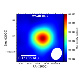
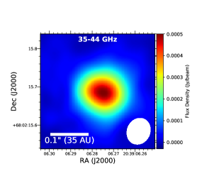
Figure 1: Images of L1157 MMS The sources are clearly resolved in both frequency ranges with respect to the beam, but details of the structure cannot be discerned at this resolution. The main impact of self-calibration on images at this resolution is a higher peak intensity in both images as compared to the non-self-calibrated data. The values for the beam sizes in each image are provided in Table 3.

L1157 MMS is clearly detected in our Q and Ka-band imaging in A-configuration. We show images of L1157 MMS in Figure 1 generated with robust=2 from the combined Q and Ka-band data, providing the best sensitivity. The source has a similar morphology when imaged with the full bandwidth vs. only the 35 to 44 GHz range, also shown in Figure 1. The source is resolved compared to the synthesized beam, and the peak intensity in the combined Q and Ka-band image is 0.47 mJy beam^-1, while the integrated flux density is $\sim$1.1 mJy, further demonstrating that the source is resolved.

We made images for the full range of the combined Q and Ka-band data and the 35 to 44 GHz range using $robust=-0.25$ to add more weight to the longer baselines during imaging, resulting in higher resolution images. These two higher resolution images in Figure 2 show that the continuum emission is resolved into two peaks. The peak intensity of the western peak (0.27 mJy beam^-1) is about 1.3$\times$ greater than the eastern peak (0.20 mJy beam^-1). We denote the western peak as component A and the eastern peak as component B. These resolved peaks have a position angle comparable to the marginally-resolved 7.3 mm image of L1157 MMS from Tobin et al. (2013). The new data (Q and Ka-bands combined) have a factor of 2.7 lower noise and higher angular resolution than the previous observations. The improved S/N is a result of the wider bandwidth and longer integration time for the new data. We also show a comparison of the images generated with self-calibration applied and those without self-calibration applied in Figure 2. This demonstrates that the two sources are detected and resolved whether self-calibration is applied or not, but the significance of the eastern component is increased by $>$2$\sigma$ in the self-calibrated images.

The positions of the continuum sources are listed in Table 2, along with the values from the a reprocessing and analysis of the 2012 data (see Appendix), and the beams and RMS noises in each image used for the Figures are given in Table 3. The overall source position is measured using the robust=2.0 image from the combined Q and Ka-band data, while the positions of the individual resolve sources are measured from the robust=-0.25 image using the combined Q and Ka-band data. The continuum positions were fitted using the CASA task imfit, and when fitting the positions of the two continuum sources, we fixed the size of the Gaussians to the size of the synthesized beam.

The time baseline of $\sim$2.6 yr from the observations in 2012 to the new observations in 2015 enables us to calculate the proper motion of L1157 MMS as a whole (not the individual components A and B). We calculate a proper motion of 23.9$\pm$2.1 mas yr^-1 for Right Ascension and 2.3$\pm$2.0 mas yr^-1 for Declination using the coordinates from each epoch of observation.

3.1 Binary Protostar

The double-peaked morphology of the image toward L1157 MMS suggests that L1157 MMS is a proto-binary system with a separation of 0$\farcs$044$\pm$0.002 ($\sim$16 au). This is one of the closest Class 0 proto-binary systems known. Its angular and physical separation is smaller than the most compact multiple systems observed by Tobin et al. (2016, 2021) in the VLA and ALMA Nascent Disk and Multiplicity (VANDAM) Surveys. We examined the data in several ways to ensure the robustness of our detection detection of two sources within L1157 MMS, and we outline the additional analysis in the Appendix.

3.2 Polarization Upper Limits

As part of our high-resolution observations, we also examined the polarimetry toward L1157 MMS in Q-band. We constructed Stokes IQUV cubes using Natural weighting and with a uv-taper at 1000 k$\lambda$ to focus on larger angular scales. However, on the size scales probed in those images (0$\farcs$06 and 0$\farcs$14), we do not detect significant Stokes Q or U emission. Thus, we can only provide 3$\sigma$ upper limits on the total polarized peak intensity of 0.1 mJy beam^-1 and 0.15 mJy beam^-1 for the 0$\farcs$06 and 0$\farcs$14 beams, respectively. While Ka-band was also calibrated for polarimetry, we only provide results for Q-band since it has the brightest dust emission. We do not show the Stokes Q and U images for the sake of brevity, but describe their properties in Table 3.

3.3 Millimeter to Radio Spectrum

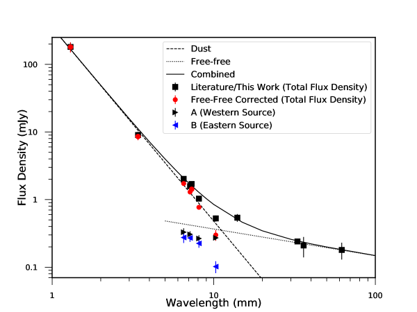
Figure 3: Radio spectrum of L1157 MMS. The black points are the raw measurements of the flux densities toward L1157 MMS as a whole, including both components. The spectrum is modeled using two power-laws, one describing the free-free emission (dotted line) and the dust emission (dashed line). The black line is the sum of the dust and free-free fits. The red points show the emission with the estimated free-free emission subtracted. Lastly, the individual flux densities for the A (black right pointing triangles) and B (blue left pointing triangles) components are plotted. The uncertainties shown on each flux density measurement are statistical only.

We have updated the radio to millimeter spectrum of L1157 MMS with these new data, sampling 27 to 48 GHz. Furthermore, we also report the flux densities of the two continuum peaks detected that likely trace a proto-binary system. We measured the integrated flux densities in several wavelength bins, but using lower angular resolution images with the beams approximately matched to the Naturally-weighted beam at 44 to 48 GHz (see Table 3 and the Per 4 GHz - Binary Unresolved images for more detail). We measured the flux densities using Gaussian fitting with the CASA task imfit to measure the integrated flux densities; the results from Gaussian fitting are consistent within uncertainties to flux densities extracted from an aperture encompassing all emission. The flux densities are listed in Table 4, along with flux densities from the literature. The radio spectrum shown in Figure 3 has the typical form expected for a protostar, dust-dominated emission at the short wavelengths ($\lambda$ $<$1 cm) and free-free-dominated emission at longer wavelengths ($\lambda$ $>$1 cm).

We fit the radio spectrum with two power-laws, one corresponding to the long-wavelength emission and another corresponding to the shorter wavelength emission. We first fit the free-free only portion of the spectrum at 3 cm to 6 cm since the contribution of dust emission to those flux densities is negligible. The free-free portion of the spectrum can be described by the function $F_{\nu,ff}$ = 0.37($\nu/30~{}GHz)^{0.4\pm 0.15}$. We then subtracted this estimated free-free emission from all the data at $\lambda$ $<$ 1 cm. Using the free-free corrected data, we fitted the slope of the dust emission, finding $F_{\nu,dust}$ = 0.48($\nu/30~{}GHz)^{2.87\pm 0.1}$. Then we plot the sum of these two power-laws in Figure 3, and this function matches the total flux densities of the source from 0.1 cm to 6 cm.

We also measured the flux densities toward the two resolved sources. We used the imfit task in CASA to fit two Gaussians simultaneously. We fixed the source sizes to correspond to the synthesized beams in each image to limit the free parameters in the fit and to avoid fitting the extended emission. However, the residuals are negligible after subtracting the two point sources indicating that these higher resolution images (Table 3; Per 4 GHz - Binary Resolved images) are recovering less flux density than those with lower resolution (Table 3 and the Per 4 GHz - Binary Unresolved images). As such, the flux densities of the two resolved components are significantly lower than the integrated flux densities shown in Figure 3. Their spectral slopes are also more shallow, at least from 6.5 mm to 8.1 mm, which could be due to the free-free emission contributing a more significantly fraction to the total emission for each component. Then, at 10.3 mm the flux density for B is low compared to the other measurements, while the flux density for A is comparable to the 8.1 mm flux density. This result could be due to low S/N for B at 10.3 mm where it appears less distinct than in the other bands.

3.4 Dust Mass

The integrated flux density in the observed bands also enables us to estimate the mass of the emitting material with the assumption of optically thin and isothermal dust emission using the equation

$$M_{dust}=\frac{F_{\nu}d^{2}}{\kappa_{\nu}B_{\nu}(T_{dust})}.$$ (1)

$F_{\nu}$ is the integrated flux density at the chosen frequency, $d$ is the distance to the source, $\kappa_{\nu}$ is the dust mass opacity at the same frequency as $F_{\nu}$, and $B_{\nu}(T_{dust})$ is the Planck function. We use the integrated flux density of 1.7 mJy at 6.5 mm that corresponds to the flux density with the estimated free-free contribution removed (Table 4). We adopt a dust temperature of $T_{dust}$=43 K (L/L_bol)^0.25 (Tobin et al., 2020) which accounts for the luminosity dependence of the average dust temperature of the protostellar disk. L_bol is 7.6 L_☉ (Green et al., 2013) when scaled to the revised distance of 352 pc, resulting in an estimated $T_{dust}$ $\sim$ 71 K, and we adopt $\kappa_{\nu}$=0.2 cm² g^-1 (Woitke et al., 2016) at 6.5 mm. With these assumptions, we calculate that the dust mass of L1157 MMS is 372 M_⊕ of dust, and if one adopts a dust to gas mass ratio of 1:100, the total mass is is calculated to be 0.11 M_☉. This calculated mass specifically applies to the size scale of the emission detected here, all of which is contained within a radius of 50 au from the protostars. Finally, comparable mass estimates can also be derived from the 1.3 mm flux densities with the same assumptions, aside from the 1.3 mm dust mass opacity.

4 Discussion

L1157 MMS is one of the most compact Class 0 multiple systems. Its separation of $\sim$16 au is more compact than the detections found in large surveys for protostellar multiplicity (Tobin et al., 2016, 2021). The wealth of complementary data on this system also enables us to put this detection in the context of the known envelope properties (Looney et al., 2007; Chiang et al., 2012; Maury et al., 2019), envelope rotation at small and larger scales (Tobin et al., 2011; Gaudel et al., 2020), the outflow (Bachiller et al., 2001; Kwon et al., 2015; Podio et al., 2016), and magnetic fields (Stephens et al., 2013).

4.1 Inner Disk or Binary?

An obvious question to ask is whether our detection of two peaks could simply be an inner disk or must it be a binary protostar system. If the disk were a smooth circumstellar disk around a single source, it is expected to appear centrally peaked. Other edge-on Class 0 disks observed with the VLA at comparable resolution appear centrally-peaked (e.g., Segura-Cox et al., 2016, 2018; Lin et al., 2021). However, if the disk had an inner cavity with a radius of approximately half the distance between the components in L1157 MMS, it could present a similar appearance to a binary system with two disks. But then the cause of the central cavity would also require explanation, which would again point to a binary system with an even closer separation. Also, even in the case of a disk with a large central cavity, we expect that the centroid of the free-free emission will be in between the two dust peaks, which is not seen (see Appendix). Moreover, the flux density of the western source does not decrease in the 35-39 GHz range, it is rather constant or slightly increased at 27-31 GHz (Figure 3). This is in line with free-free emission increasing at longer wavelengths. To ultimately confirm that the free-free peaks have positions coincident the components observed at Q and Ka-bands will require higher-resolution data at longer wavelengths.

Although we cannot fully rule-out a disk with a central inner cavity, we do not favor this interpretation. Moreover, if our observations were tracing a single disk with such a large cavity, it would be difficult to reconcile the large gap from the inner disk to the protostar with the previously observed large outflow rate of the protostar. For that reason, we posit that L1157 MMS is a 16 au binary system, and we expect that the compact emission toward each component is tracing an unresolved circumstellar disk in addition to some free-free emission.

4.2 Formation Mechanism

The presence of such a close binary in L1157 MMS raises immediate questions as to how it formed in this young system. L1157 MMS has a well-ordered magnetic field exhibiting a clear hourglass shape as observed via polarimetry at 1.3 mm from the Combined Array for Millimeter Astronomy (CARMA) by Stephens et al. (2013). The envelope specific angular momentum profile measured by Gaudel et al. (2020) clearly shows a decrease in specific angular momentum from large to small radii, possibly indicating that magnetic braking has removed angular momentum from the system. Thus, the binary system in L1157 MMS must have formed in the absence of both strong rotation and a large disk.

One possibility is that the companion formed at a larger initial separation, and the accretion of low angular momentum material drove the separation smaller (Zhao & Li, 2013). The specific angular momentum of the binary system is $\sim$8$\times$10^-5 km s^-1 pc, assuming each component is 0.02 M_☉ (Kwon et al., 2015) estimated from their C¹⁸O kinematic data that showed very low rates of rotation on $<$1000 au scales. This value is consistent with the specific angular momentum profile extrapolated to smaller radii by Gaudel et al. (2020). Thus, the scenario of forming at larger radii and migrating is possible, and a companion could migrate from 100s of au to 10s of au on time scales of a few 10s of kyr (Zhao & Li, 2013). However, the plausibility of this scenario is uncertain because the most practical method of fragmenting the envelope on these scales would be turbulent fragmentation (Offner et al., 2010; Lee et al., 2019), but the envelope itself has very narrow line widths ($<$1 km s^-1, Tobin et al., 2011) and the line width increases in the inner envelope appear to be associated with the outflow rather than internal kinematics. There is also no evidence of a second outflow having been launched within several hundred au of the main protostars, which could have served as a signpost of past star formation. Instead, there is primarily evidence for twin jets with an overlapping origin point (Kwon et al., 2015, see Section 4.3).

The other possibility is that the companion formed near its current location within a small disk. If we assume that the total flux density at 6.8 mm corresponds to the emission from the original single disk, then the disk mass was $\sim$0.11 M_☉. We can estimate the stability of that disk around L1157 MMS using a simplified form of Toomre’s Q parameter from Kratter & Lodato (2016)

$$Q\approx 2\frac{M_{*}}{M_{d}}\frac{H}{R}.$$ (2)

$M_{*}$ is the mass of the protostar (in solar masses), $M_{d}$ is the total mass of the disk (gas and dust) in solar masses, H is the vertical scale height of the disk, and R is the radius of the disk. The vertical scale height $H$ is equivalent of $c_{s}$/$\omega$; $c_{s}$ is the sound speed, and $\omega$ is the angular velocity at the radius where Q is being measured. We use an estimated rotation rate of the two protostars of 1.0 km s^-1 at 16 au, translating to $\omega$ = 4$\times$10^-10 s^-1, and we use $c_{s}\sim$0.54 km s^-1 at a temperature of $\sim$71 K. Then the total $M_{*}$ is estimated to be 0.04 M_☉ (Kwon et al., 2015). Plugging these terms into the equation yields Q$\sim$0.4, indicating that the original inner disk around L1157 MMS could have been gravitationally unstable. However, uncertainties in translating the 6.8 mm flux density to total disk mass, the protostar mass, and the disk temperature make this a very tentative estimate, but this calculation does demonstrate that the inner disk perhaps had enough mass to fragment. The disk in the past could have had even higher mass prior to fragmentation, much of which could have been accreted to form the a secondary protostar.

The formation of the companion in situ would require that a compact, gravitationally unstable disk formed within L1157 MMS. Moreover, if the observational constraints on the magnetic field and rotation rates are correct, the rotation of the envelope could have undergone significant magnetic braking, restricting disk formation to a relatively small radius where non-ideal MHD effects like Ohmic dissipation and the Hall effect could dissipate the magnetic flux and enable disk formation (e.g., Li et al., 2014). Simulations of disk formation within magnetically-dominated envelopes do show that formation of gravitationally unstable disks with radii of only 10s of au are indeed possible (Zhao et al., 2018; Lam et al., 2019; Xu & Kunz, 2021). Therefore, the idea that the companion formed in situ via fragmentation of a compact, gravitationally unstable disk is plausible.

4.3 Binary and Outflow

One of the most obvious features of the large-scale outflow from L1157 MMS is that it appears to be precessing. This was apparent in the earlier data from Gueth et al. (1996); Bachiller et al. (2001) and in the Spitzer Space Telescope images of the shock-excited molecular hydrogen emission with a ribbon-like appearance (Looney et al., 2007). More recently, Kwon et al. (2015) modeled the outflow as two precessing jets, and Podio et al. (2016) modeled the outflow as a single precessing jet.

The two jet fit from Kwon et al. (2015) implicitly assumed that there is a binary system launching the jet and that the binary system is causing tidal precession. From the modeling, they found that for the two jet fit the orbital period is (50–370) M${}_{1}^{-1/4}$yr, while for Jet 2 the orbital period is (60–450) M${}_{1}^{-1/4}$yr. The orbital radius for Jet 1 is (13–52) M${}_{1}^{1/3}$ au and for Jet 2 the orbital radius is (15–60) M${}_{1}^{1/3}$ au. The mass of each component was assumed to be 0.02 M_☉, totaling 0.04 M_☉ (see section 4.2). The lower range of orbital radii fit are consistent with the observed separation of the two continuum sources. Even if the overall mass of the protostars is higher, the orbital radii of the jets only increase slowly with increasing mass.

The orbital motion of the binary alone does not cause the outflow precession as the orbital periods are much shorter than the apparent outflow precession. Thus, Kwon et al. (2015) found that the precession periods are $\sim$5200 and $\sim$7600 yr for the two jets. On the other hand, Podio et al. (2016) finds an outflow precession period of 1640 yr. The assumption of a single outflow in Podio et al. (2016) makes it necessary for the outflow to precess faster in order to match the observations.

The orbital radii and periods of the jets are compatible with the projected separation of the two continuum sources that we detect. Moreover, the projected separation could be smaller than the full semi-major axis since we do not know where in the orbital path we are observing the system. Therefore, the observed parameters of the binary system are completely consistent with the constraints from modeling of the outflows.

4.4 Context with other Binary systems

L1157 MMS is the most compact known Class 0 proto-multiple system resolved in dust continuum emission. Other similarly compact proto-multiple systems are IRAS 03292-3039 (Per-emb 2) (24 au), HOPS-361-E (22 au), BHB2007 11 (28 au), Per-emb 18 (26 au), VLA1623A (30 au), and L483 (30 au) (Tobin et al., 2016; Harris et al., 2018; Alves et al., 2019; Tobin et al., 2021, Cox et al. subm.). The protostar IRAS 16293-2422A has also had a number of components and potential substructures resolved in submillimeter to centimeter radio continuum (e.g., Hernández-Gómez et al., 2019; Maureira et al., 2020; Oya et al., 2021, and references therein) that can have separations as close as $\sim$0$\farcs$1. However, the most robust components that are likely to be true protostellar sources are the A1 and A2 sources that are $\sim$54 au in projected separation.

The primary difference between L1157 MMS and these other systems, other than its very close separation, is the presence of obvious rotation toward most of them (except HOPS-361-E), likely corresponding to circumbinary disk emission or at least a rotating envelope (Tobin et al., 2019; Alves et al., 2019). L1157 MMS on the other hand shows no signs of strong rotation on $<$ 1000 au scales as discussed in Sections 1 and 4.2. Thus, L1157 MMS demonstrates that fragmentation and close multiple formation is still possible in cases where the dynamics of the collapse may be regulated by magnetic fields.

We emphasize that the case of L1157 MMS is distinct from NGC 1333 IRAS 4A (IRAS4A), which is another proto-binary with a well-ordered magnetic field (Girart et al., 2006; Cox et al., 2015; Ko et al., 2020). The binary in IRAS4A has a much wider separation of $\sim$540 au vs. 16 au for L1157 MMS. Furthermore, the magnetic field in IRAS4A is misaligned with respect to the outflows from the IRAS4A sources (Hull et al., 2014; Chuang et al., 2021), where as the magnetic field in L1157 MMS is aligned with the outflow.

The presence of such a close binary system in L1157 MMS demonstrates a pathway for the formation of binary systems with separations $<$10 au. Currently the only evidence for protostellar multiple systems with separations $<$10 au are a few radial velocity observations of Class I protostars (Viana Almeida et al., 2012) and the indirect evidence from variability in one system that is interpreted as binary-modulated pulsed accretion (Muzerolle et al., 2013). More-evolved Class II and Class III pre-main-sequence systems, on the other hand, have multiplicity characteristics at $<$10 au consistent with field stars (Kounkel et al., 2019). Thus, it is an open question whether these $<$10 au companions first formed at much larger separations (many 10s to 100s of au) and migrated inward or if they could have formed closer in. The 16 au binary in L1157 at least suggests that formation near 10 au separation is possible in Class 0 systems and migration of clumps and/or fully formed companions could easily populate $<$10 au separations (e.g., Zhu et al., 2012; Zhao & Li, 2013).

5 Conclusions

We have discovered a compact proto-binary system forming within L1157 MMS using observations at Q (6.8 mm) and Ka-bands (9 mm) with the VLA. It is currently the most compact known Class 0 proto-binary system, with a projected separation of $\sim$16 au. The mass of the inner envelope and disk surrounding the protostars (within a 50 au radius) is estimated to be $\sim$0.11 M_☉, using simple assumptions for converting dust emission to mass. The L1157 MMS system as a whole has a large flattened envelope with very weak rotation from 10000 au to $\sim$200 au scales probed by both N₂H⁺ and C¹⁸O emission (Tobin et al., 2011; Kwon et al., 2015; Gaudel et al., 2020), and the system has an observed poloidal magnetic field (Stephens et al., 2013). Thus, L1157 MMS also demonstrates that the formation of compact binary systems is possible, even when magnetic fields may be dynamically important to the collapse and disk formation. Finally, of the known multiple protostar systems with separations $<$ 30 au that have had their inner envelope/disk kinematics characterized, L1157 MMS stands alone in being the only one without clear organized rotation surrounding the binary.

Appendix A Robustness of the Binary

We performed several additional tests on the data to confirm the robustness of the binary detection. We first re-reduced the data from (Tobin et al., 2013) and show the data in Figure 4. These data were Q-band, had 2 GHz of bandwidth, and only include the A-configuration data from the paper. The image clearly shows that L1157 MMS is extended, in the same direction as detected in Figures 2, showing evidence for two peaks. However, the eastern source is not a distinct point source owing to the lower sensitivity of those data, but like the data in Figure 2 the western source is brighter.

We then further analyzed the data presented in this paper to examine the robustness of the observed binary. To ensure that the detection is robust across our observed frequency range, we separately imaged 4 GHz chunks of the observed bands from the combined dataset. At each wavelength we tuned the $robust$ parameter to provide similar beams in each frequency interval (Table 3). We show the images in Figure 5, and each frequency interval similarly shows a double peaked structure. The lowest frequency band only marginally resolves the structure because of its inherently lower angular resolution. Moreover, the peak intensity of the western peak is $\sim$1.5 to 2$\times$ brighter than the eastern peak.

We next imaged each observation from Table 1 separately, using the full Q and Ka-band bandwidth (Figure 6). While there is some variation in the observed structure in each epoch, which is expected from phase noise, there is a double-peaked structure detected in all epochs of observation. Thus, the two peaks resolved in the new data, in conjunction with a similar structure resolved in the previous data, and two peaks resolved with different VLA bands, lead us to conclude that this resolved structure is robust and is not an artifact of low S/N or phase noise in the data.

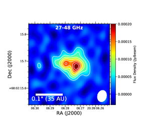
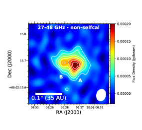
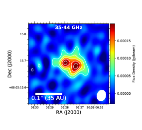
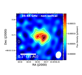
Figure 2: Images of L1157 MMS generated using the full combined Q and Ka-bands (top) and only the 35 to 44 GHz spectral range (bottom) with a robust parameter of -0.25. We also show the self-calibrated images (left) in comparison to the images without self-calibration (right). The binary clearly stands out in the self-calibrated images better than the non-self-calibrated images, with its significance increasing by $>$2$\sigma$. The contours in the right panels start at 3$\sigma$ and increase on 2$\sigma$ intervals; values for $\sigma$ and the beam sizes in each image are provided in Table 3. The noise and beam sizes are approximately the same for the self-calibrated and non-self-calibrated images.

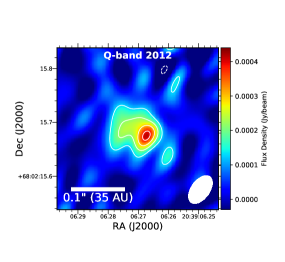
Figure 4: Images of L1157 MMS at 41 GHz from the observations in 2012. This is re-reduced from the data presented in Tobin et al. (2013). This image was produced with robust=-0.5. The contours are drawn at -3, 3, 5, 7, 9$\sigma$, where $\sigma$=43 $\mu$Jy beam^-1. The beam is 0$\farcs$058$\times$0$\farcs$033. The morphology is consistent with the newer data, lending confidence that the second continuum peak is a robust feature.

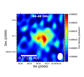
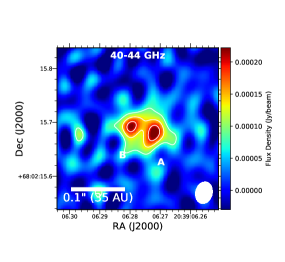
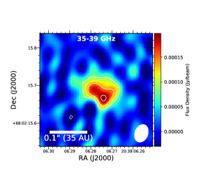
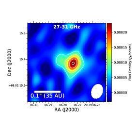
Figure 5: Images of L1157 MMS in 4 GHz chunks across the observed bands. The contours start at $\pm$3$\sigma$ and increase on 2$\sigma$ intervals, where $\sigma$ and the beams for each image are provided in Table 3.

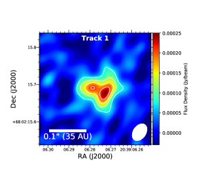
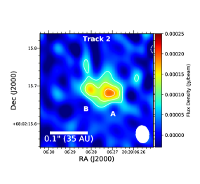
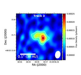
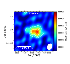
Figure 6: Images of L1157 MMS from each of the 4 epochs of observation using the combined Q and Ka-band spectral range. The contours start at $\pm$3$\sigma$ and increase on 2$\sigma$ intervals, where $\sigma$ and the beams for each image are provided in Table 3.

Table 1: VLA Observation Log

Fields	Date	Duration	Calibrators
		(hr)	Bandpass, Flux, Complex Gain
L1157	2015 Jun 26	2.5	3C84, 3C48, J2006+6424
L1157	2015 Jun 30	2.5	3C84, 3C48, J2006+6424
L1157	2015 Jul 01	2.5	3C84, 3C48, J2006+6424
L1157	2015 Sep 21	2.5	3C84, 3C48, J2006+6424

Note. —

Table 2: Source Positions

Source	Right Ascension	Declination
	(J2000)	(J2000)
2015 Data
L1157 MMS	20:39:06.2746$\pm$0.0001	+68:02:15.6853$\pm$0.001
L1157 MMS-A	20:39:06.2724$\pm$0.0001	+68:02:15.680$\pm$0.002
L1157 MMS-B	20:39:06.2798$\pm$0.0001	+68:02:15.693$\pm$0.002
2012 Data
L1157 MMS	20:39:06.2704$\pm$0.0001	+68:02:15.683$\pm$0.002
L1157 MMS-A	20:39:06.2675$\pm$0.0001	+68:02:15.674$\pm$0.002
L1157 MMS-B	20:39:06.2747$\pm$0.0002	+68:02:15.693$\pm$0.003

Note. —

Table 3: Image Properties

Image	Track	Stokes	Robust, Taper	Beam Size	RMS	Freq. Range	$\lambda$	Figure
				(″)	($\mu$Jy beam-1)	(GHz)	(mm)
2015 Data
1. Q+Ka	All Tracks	I	2.0	0.074$\times$0.060	6.9	27 - 48	8.45	1
2. Q+Ka	All Tracks	I	-0.25	0.044$\times$0.034	12.6	27 - 48	8.45	2
3. Q+Ka	All Tracks	I	2.0	0.068$\times$0.057	9.8	35 - 44	7.6	1
4. Q+Ka	All Tracks	I	-0.25	0.043$\times$0.033	17.8	35 - 44	7.6	2
5. Q	All Tracks	I	2.0	0.061$\times$0.050	24.2	40 - 48	6.8	$\cdots$
6. Q	All Tracks	Q	2.0	0.061$\times$0.050	24.2	40 - 48	6.8	$\cdots$
7. Q	All Tracks	U	2.0	0.061$\times$0.050	23.2	40 - 48	6.8	$\cdots$
8. Q	All Tracks	I	2.0, 1000 k$\lambda$	0.14$\times$0.12	38.8	40 - 48	6.8	$\cdots$
9. Q	All Tracks	Q	2.0, 1000 k$\lambda$	0.14$\times$0.12	35.2	40 - 48	6.8	$\cdots$
10. Q	All Tracks	U	2.0, 1000 k$\lambda$	0.14$\times$0.12	31.8	40 - 48	6.8	$\cdots$
Per 4 GHz - Binary Resolved
11. Q	All Tracks	I	0.0	0.043$\times$0.032	34.5	44 - 48	6.52	5
12. Q	All Tracks	I	0.0	0.041$\times$0.031	27.8	40 - 44	7.14	5
13. Ka	All Tracks	I	-0.5	0.049$\times$0.035	28.7	35 - 39	8.1	5
14. Ka	All Tracks	I	-0.5	0.058$\times$0.043	21.5	27 - 31	10.3	5
Per 4 GHz - Binary Unresolved
15. Q	All Tracks	I	2.0	0.062$\times$0.049	23.6	44 - 48	6.52	$\cdots$
16. Q	All Tracks	I	1.5	0.060$\times$0.051	15.8	40 - 44	7.14	$\cdots$
17. Ka	All Tracks	I	0.5	0.062$\times$0.049	14.3	35 - 39	8.1	$\cdots$
18. Ka	All Tracks	I	0.0	0.063$\times$0.046	14.9	27 - 31	10.3	$\cdots$
Per Observation Images
19. Q+Ka	Track 1	I	-0.25	0.051$\times$0.034	22.8	27 - 47	8.1	6
20. Q+Ka	Track 2	I	-0.25	0.047$\times$0.035	24.9	27 - 48	8.0	6
21. Q+Ka	Track 3	I	-0.25	0.048$\times$0.034	23.1	27 - 48	8.0	6
22. Q+Ka	Track 4	I	-0.25	0.048$\times$0.036	21.8	27 - 48	8.0	6
2012 Data
23. Q	All Tracks	I	-0.5	0.058$\times$0.033	42.4	40 - 42	7.3	4

Note. — Here we describe all the images used in the analysis presented here. Note that we do not show all images in the paper for the sake of brevity, but we include their properties since they were used to measure flux densities and/or analyzed the upper limits on polarized flux density.

Table 4: Flux densities

Wavelength	Flux Density	Peak Intensity	Image Robust	Reference	Table 3 Image
(mm)	(mJy)	(mJy beam-1)
Combined
1.3	181$\pm$30	98.5	$\cdots$	3	$\cdots$
3.4	9.0$\pm$1.0	6.8	$\cdots$	3	$\cdots$
6.52	2.0$\pm$0.1 (1.7)	0.51	2.0	1	15
7.14	1.6$\pm$0.1 (1.3)	0.47	1.5	1	16
7.3	1.7$\pm$0.1	0.49	2.0	2	$\cdots$
8.45 (27-48 GHz)	1.1$\pm$0.04	0.47	2.0	1	1
8.1	1.0$\pm$0.05 (0.77)	0.34	0.5	1	17
10.3	0.53$\pm$0.05 (0.30)	0.23	0.0	1	18
14	0.54$\pm$0.07	0.31	2.0	2	$\cdots$
33	0.24$\pm$0.02	0.21	2.0	2	$\cdots$
36	0.21$\pm$0.07	0.21	2.0	2	$\cdots$
62	0.18$\pm$0.05	0.19	2.0	2	$\cdots$
A (western) source
6.52	0.33$\pm$0.05	0.33	0.0	1	11
7.14	0.31$\pm$0.03	0.31	0.0	1	12
8.1	0.27$\pm$0.03	0.27	-0.5	1	13
8.45 (27-48 GHz)	0.27$\pm$0.03	0.27	-0.25	1	2
10.3	0.27$\pm$0.02	0.27	-0.5	1	14
B (eastern) source
6.52	0.27$\pm$0.05	0.27	0.0	1	11
7.14	0.27$\pm$0.03	0.27	0.0	1	12
8.1	0.23$\pm$0.03	0.22	-0.5	1	13
8.45 (27-48 GHz)	0.20$\pm$0.02	0.2	-0.25	1	2
10.3	0.1$\pm$0.02	0.1	-0.5	1	14

Note. — Values presented in this table are the result of Gaussian fitting to the source(s). The fits to the A and B source flux densities have their major and minor axes fixed to the size of the synthesized beam at each wavelength. The values in parentheses in the Flux Density column have their estimated free-free contribution subtracted. References: 1 - This work, 2 - (Tobin et al., 2013), 3 - (Chiang et al., 2012). The last column, Table 3 Image refers to the image number in Table 3 that the flux densities were derived from.

References

- Allen et al. (2003) Allen, A., Li, Z.-Y., & Shu, F. H. 2003, ApJ, 599, 363, doi: 10.1086/379243
- Alves et al. (2019) Alves, F. O., Caselli, P., Girart, J. M., et al. 2019, Science, 366, 90, doi: 10.1126/science.aaw3491
- André et al. (1993) André, P., Ward-Thompson, D., & Barsony, M. 1993, ApJ, 406, 122, doi: 10.1086/172425
- Astropy Collaboration et al. (2018) Astropy Collaboration, Price-Whelan, A. M., Sipőcz, B. M., et al. 2018, The Astropy Project: Building an Open-science Project and Status of the v2.0 Core Package, doi: 10.3847/1538-3881/aabc4f
- Bachiller et al. (1993) Bachiller, R., Martin-Pintado, J., & Fuente, A. 1993, ApJ, 417, L45, doi: 10.1086/187090
- Bachiller et al. (2001) Bachiller, R., Pérez Gutiérrez, M., Kumar, M. S. N., & Tafalla, M. 2001, A&A, 372, 899, doi: 10.1051/0004-6361:20010519
- Basu & Mouschovias (1995) Basu, S., & Mouschovias, T. C. 1995, ApJ, 452, 386, doi: 10.1086/176310
- Brogan et al. (2018) Brogan, C. L., Hunter, T. R., & Fomalont, E. B. 2018, arXiv e-prints, arXiv:1805.05266. https://arxiv.org/abs/1805.05266
- Chapman et al. (2013) Chapman, N. L., Davidson, J. A., Goldsmith, P. F., et al. 2013, ApJ, 770, 151, doi: 10.1088/0004-637X/770/2/151
- Chiang et al. (2012) Chiang, H.-F., Looney, L. W., & Tobin, J. J. 2012, ApJ, 756, 168, doi: 10.1088/0004-637X/756/2/168
- Chiang et al. (2010) Chiang, H.-F., Looney, L. W., Tobin, J. J., & Hartmann, L. 2010, ApJ, 709, 470, doi: 10.1088/0004-637X/709/1/470
- Chuang et al. (2021) Chuang, C.-Y., Aso, Y., Hirano, N., Hirano, S., & Machida, M. N. 2021, ApJ, 916, 82, doi: 10.3847/1538-4357/abfdbb
- Cox et al. (2015) Cox, E. G., Harris, R. J., Looney, L. W., et al. 2015, ApJ, 814, L28, doi: 10.1088/2041-8205/814/2/L28
- Galli & Shu (1993) Galli, D., & Shu, F. H. 1993, ApJ, 417, 220, doi: 10.1086/173305
- Gaudel et al. (2020) Gaudel, M., Maury, A. J., Belloche, A., et al. 2020, A&A, 637, A92, doi: 10.1051/0004-6361/201936364
- Girart et al. (2006) Girart, J. M., Rao, R., & Marrone, D. P. 2006, Science, 313, 812, doi: 10.1126/science.1129093
- Green et al. (2013) Green, J. D., Evans, Neal J., I., Jørgensen, J. K., et al. 2013, ApJ, 770, 123, doi: 10.1088/0004-637X/770/2/123
- Greenfield et al. (2013) Greenfield, P., Robitaille, T., Tollerud, E., et al. 2013, ASCL. http://ascl.net/1304.002
- Gueth et al. (1996) Gueth, F., Guilloteau, S., & Bachiller, R. 1996, A&A, 307, 891
- Harris et al. (2018) Harris, R. J., Cox, E. G., Looney, L. W., et al. 2018, ApJ, 861, 91, doi: 10.3847/1538-4357/aac6ec
- Hernández-Gómez et al. (2019) Hernández-Gómez, A., Loinard, L., Chandler, C. J., et al. 2019, ApJ, 875, 94, doi: 10.3847/1538-4357/ab0c97
- Hull et al. (2014) Hull, C. L. H., Plambeck, R. L., Kwon, W., et al. 2014, ApJS, 213, 13, doi: 10.1088/0067-0049/213/1/13
- Ko et al. (2020) Ko, C.-L., Liu, H. B., Lai, S.-P., et al. 2020, ApJ, 889, 172, doi: 10.3847/1538-4357/ab5e79
- Kounkel et al. (2019) Kounkel, M., Covey, K., Moe, M., et al. 2019, AJ, 157, 196, doi: 10.3847/1538-3881/ab13b1
- Kratter & Lodato (2016) Kratter, K., & Lodato, G. 2016, ARA&A, 54, 271, doi: 10.1146/annurev-astro-081915-023307
- Kwon et al. (2015) Kwon, W., Fernández-López, M., Stephens, I. W., & Looney, L. W. 2015, ApJ, 814, 43, doi: 10.1088/0004-637X/814/1/43
- Lam et al. (2019) Lam, K. H., Li, Z.-Y., Chen, C.-Y., Tomida, K., & Zhao, B. 2019, MNRAS, 489, 5326, doi: 10.1093/mnras/stz2436
- Lee et al. (2019) Lee, A. T., Offner, S. S. R., Kratter, K. M., Smullen, R. A., & Li, P. S. 2019, ApJ, 887, 232, doi: 10.3847/1538-4357/ab584b
- Li et al. (2014) Li, Z. Y., Banerjee, R., Pudritz, R. E., et al. 2014, in Protostars and Planets VI, ed. H. Beuther, R. S. Klessen, C. P. Dullemond, & T. Henning, 173, doi: 10.2458/azu_uapress_9780816531240-ch008
- Lin et al. (2021) Lin, Z.-Y. D., Lee, C.-F., Li, Z.-Y., Tobin, J. J., & Turner, N. J. 2021, MNRAS, 501, 1316, doi: 10.1093/mnras/staa3685
- Looney et al. (2007) Looney, L. W., Tobin, J. J., & Kwon, W. 2007, ApJ, 670, L131, doi: 10.1086/524361
- Maureira et al. (2020) Maureira, M. J., Pineda, J. E., Segura-Cox, D. M., et al. 2020, ApJ, 897, 59, doi: 10.3847/1538-4357/ab960b
- Maury et al. (2019) Maury, A. J., André, P., Testi, L., et al. 2019, A&A, 621, A76, doi: 10.1051/0004-6361/201833537
- McMullin et al. (2007) McMullin, J. P., Waters, B., Schiebel, D., Young, W., & Golap, K. 2007, in Astronomical Society of the Pacific Conference Series, Vol. 376, Astronomical Data Analysis Software and Systems XVI, ed. R. A. Shaw, F. Hill, & D. J. Bell, 127
- Muzerolle et al. (2013) Muzerolle, J., Furlan, E., Flaherty, K., Balog, Z., & Gutermuth, R. 2013, Nature, 493, 378, doi: 10.1038/nature11746
- Offner et al. (2010) Offner, S. S. R., Kratter, K. M., Matzner, C. D., Krumholz, M. R., & Klein, R. I. 2010, ApJ, 725, 1485, doi: 10.1088/0004-637X/725/2/1485
- Oya et al. (2021) Oya, Y., Watanabe, Y., López-Sepulcre, A., et al. 2021, ApJ, 921, 12, doi: 10.3847/1538-4357/ac0a72
- Podio et al. (2016) Podio, L., Codella, C., Gueth, F., et al. 2016, A&A, 593, L4, doi: 10.1051/0004-6361/201628876
- Robitaille & Bressert (2012) Robitaille, T., & Bressert, E. 2012, APLpy: Astronomical Plotting Library in Python, Astrophysics Source Code Library. http://ascl.net/1208.017
- Segura-Cox et al. (2016) Segura-Cox, D. M., Harris, R. J., Tobin, J. J., et al. 2016, ApJ, 817, L14, doi: 10.3847/2041-8205/817/2/L14
- Segura-Cox et al. (2018) Segura-Cox, D. M., Looney, L. W., Tobin, J. J., et al. 2018, ApJ, 866, 161, doi: 10.3847/1538-4357/aaddf3
- Stephens et al. (2013) Stephens, I. W., Looney, L. W., Kwon, W., et al. 2013, ApJ, 769, L15, doi: 10.1088/2041-8205/769/1/L15
- Tobin et al. (2011) Tobin, J. J., Hartmann, L., Chiang, H.-F., et al. 2011, ApJ, 740, 45, doi: 10.1088/0004-637X/740/1/45
- Tobin et al. (2013) Tobin, J. J., Chandler, C. J., Wilner, D. J., et al. 2013, ApJ, 779, 93, doi: 10.1088/0004-637X/779/2/93
- Tobin et al. (2016) Tobin, J. J., Looney, L. W., Li, Z.-Y., et al. 2016, ApJ, 818, 73, doi: 10.3847/0004-637X/818/1/73
- Tobin et al. (2019) Tobin, J. J., Bourke, T. L., Mader, S., et al. 2019, ApJ, 870, 81, doi: 10.3847/1538-4357/aaef87
- Tobin et al. (2020) Tobin, J. J., Sheehan, P. D., Megeath, S. T., et al. 2020, ApJ, 890, 130, doi: 10.3847/1538-4357/ab6f64
- Tobin et al. (2021) Tobin, J. J., Offner, S. S. R., Kratter, K. M., et al. 2021, arXiv e-prints, arXiv:2111.05801. https://arxiv.org/abs/2111.05801
- Viana Almeida et al. (2012) Viana Almeida, P., Melo, C., Santos, N. C., et al. 2012, A&A, 539, A62, doi: 10.1051/0004-6361/201117703
- Woitke et al. (2016) Woitke, P., Min, M., Pinte, C., et al. 2016, A&A, 586, A103, doi: 10.1051/0004-6361/201526538
- Xu & Kunz (2021) Xu, W., & Kunz, M. W. 2021, MNRAS, 508, 2142, doi: 10.1093/mnras/stab2715
- Zhao et al. (2018) Zhao, B., Caselli, P., Li, Z.-Y., & Krasnopolsky, R. 2018, MNRAS, 473, 4868, doi: 10.1093/mnras/stx2617
- Zhao & Li (2013) Zhao, B., & Li, Z.-Y. 2013, ApJ, 763, 7, doi: 10.1088/0004-637X/763/1/7
- Zhu et al. (2012) Zhu, Z., Hartmann, L., Nelson, R. P., & Gammie, C. F. 2012, ApJ, 746, 110, doi: 10.1088/0004-637X/746/1/110
- Zucker et al. (2019) Zucker, C., Speagle, J. S., Schlafly, E. F., et al. 2019, ApJ, 879, 125, doi: 10.3847/1538-4357/ab2388