EvoKG: Jointly Modeling Event Time and Network Structure for Reasoning over Temporal Knowledge Graphs

Abstract.

How can we perform knowledge reasoning over temporal knowledge graphs (TKGs)? TKGs represent facts about entities and their relations, where each fact is associated with a timestamp. Reasoning over TKGs, i.e., inferring new facts from time-evolving KGs, is crucial for many applications to provide intelligent services. However, despite the prevalence of real-world data that can be represented as TKGs, most methods focus on reasoning over static knowledge graphs, or cannot predict future events. In this paper, we present a problem formulation that unifies the two major problems that need to be addressed for an effective reasoning over TKGs, namely, modeling the event time and the evolving network structure. Our proposed method EvoKG jointly models both tasks in an effective framework, which captures the ever-changing structural and temporal dynamics in TKGs via recurrent event modeling, and models the interactions between entities based on the temporal neighborhood aggregation framework. Further, EvoKG achieves an accurate modeling of event time, using flexible and efficient mechanisms based on neural density estimation. Experiments show that EvoKG outperforms existing methods in terms of effectiveness (up to 77% and 116% more accurate time and link prediction) and efficiency.

ACM Reference Format:
Namyong Park, Fuchen Liu, Purvanshi Mehta, Dana Cristofor, Christos Faloutsos, Yuxiao Dong. 2022. EvoKG: Jointly Modeling Event Time and Network Structure for Reasoning over Temporal Knowledge Graphs. In Proceedings of the Fifteenth ACM International Conference on Web Search and Data Mining (WSDM ’22), February 21–25, 2022, Tempe, AZ, USA. ACM, New York, NY, USA, 10 pages. https://doi.org/10.1145/3488560.3498451

1. Introduction

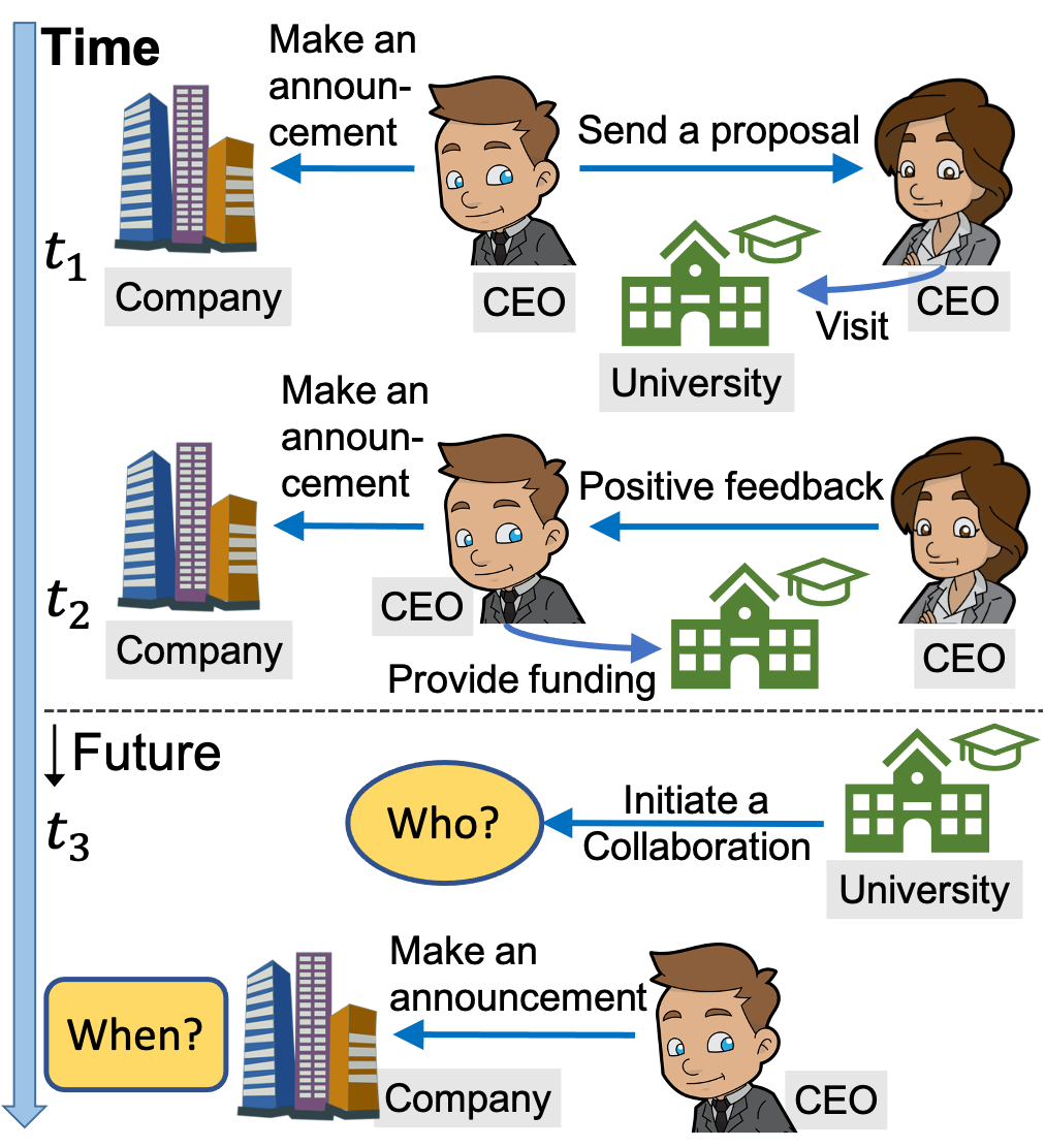
Figure 1. An example TKG, where we aim to predict temporal links and event time.

How can we perform knowledge reasoning over knowledge graphs (KGs) that continuously evolve over time? KGs (Ji et al., 2020) organize and represent facts on various types of entities and their relations. By facilitating an effective use of prior knowledge represented as a multi-relational graph, KGs power many important applications, including question answering, recommender systems, search engines, and natural language processing. Knowledge reasoning over KGs (Chen et al., 2020), the process of inferring new knowledge from existing facts in KGs, lies at the heart of these applications, as KGs are typically incomplete, with many facts missing.

Importantly, real-world events and facts are often associated with time (i.e., occurring at a specific time or valid in limited time), exhibiting complex dynamics among entities and their relations that evolve over time. Such real-world data (e.g., ICEWS (Boschee et al., 2015) and GDELT (Leetaru and Schrodt, 2013)) can be modeled as temporal knowledge graphs (TKGs), where entities are connected via timestamped edges, and two entities can have multiple interactions at different time steps, as illustrated in Figure 1. Despite the prevalence of real-world data that can be represented as TKGs, existing methods (Yang et al., 2015; Schlichtkrull et al., 2018; Dettmers et al., 2018; Sun et al., 2019) have mainly focused on reasoning over static KGs, and lack the ability to employ rich temporal dynamics available in TKGs.

Recently, a few methods have been developed for reasoning over TKGs. They mainly address two problem setups, i.e., interpolation and extrapolation. Given a TKG ranging from time $0$ to time $T$, methods for the interpolation setup (Dasgupta et al., 2018; García-Durán et al., 2018; Leblay and Chekol, 2018) infer missing facts for time $t~{}(0\leq t\leq T)$; on the other hand, those for the extrapolation setup (Trivedi et al., 2017, 2019; Jin et al., 2020) predict new facts for time $t>T$. In this paper, we focus on the extrapolation setting, which is more challenging and interesting than the other setting, as forecasting emerging events are of great importance to many applications of TKG reasoning.

In this paper, we approach the problem of TKG modeling by defining the joint probability distribution of a TKG as a product of conditionals, from which we present a problem formulation that unifies the two problem settings of existing methods, namely, modeling the event time and evolving network structure. While addressing both problems leads to learning rich, complementary information useful for an effective reasoning over TKGs, most methods deal with only either of the two, as summarized in Table 1.

Therefore, in this work, we develop EvoKG, a method that jointly addresses these two core tasks for reasoning over TKGs. We design an effective framework that can be effectively applied to each task, with only minor adaptations. Our framework performs neighborhood aggregation in a relation- and time-aware manner, and carries out recurrent event modeling in an autoregressive architecture to capture the ever-changing structural and temporal dynamics over time (F1-F3 in Table 1). Importantly, EvoKG tackles the challenging task of event time modeling, using flexible and efficient mechanisms based on neural density estimation (T2-1 and T2-2 in Table 1), which avoids the limitations of existing methods that the learned distributions are not expressive, and that the log-likelihood and expectation of event time cannot be obtained in closed form, but instead require an approximation. In summary, our contributions are as follows.

• Problem Formulation (Section 2). We present a problem formulation that unifies the two major tasks for TKG reasoning—modeling the timing of events and evolving network structure.

• Framework (Section 3). We propose EvoKG, an effective and efficient method for reasoning over TKGs that jointly addresses the two core problems (T1 and T2 in Table 1).

• Effectiveness (Section 4). Experiments show that EvoKG achieves up to 116% and 77% better link and event time prediction accuracy, respectively, than existing KG reasoning methods (Figure 2).

• Efficiency (Section 4). EvoKG efficiently processes concurrent events, achieving up to 30$\times$ and 291$\times$ speedup in training and inference, respectively, compared to the best existing method.

Reproducibility. The code and data used in this paper are available at https://namyongpark.github.io/evokg.

Table 1. EvoKG wins. EvoKG deals with both tasks (T1-T2) for reasoning over TKGs, while representative baselines fail to address both. EvoKG also possesses desirable features (F1-F3) for modeling TKGs. TD: TA-DistMult (García-Durán et al., 2018). EG: EvolveGCN (Pareja et al., 2020). KE: Know-Evolve (Trivedi et al., 2017). RN: RE-Net (Jin et al., 2020).

TD EG KE RN EvoKG   T1. Modeling evolving network structure ✓ ✓ ✓ TextRenderingMode=FillStroke, LineWidth=.7pt, ✓     T2. Modeling event time $t$ ✓ TextRenderingMode=FillStroke, LineWidth=.7pt, ✓ • T2-1. Closed-form likelihood & expectation ✓ TextRenderingMode=FillStroke, LineWidth=.7pt, ✓ • T2-2. Flexible approximation of $p(t)$ TextRenderingMode=FillStroke, LineWidth=.7pt, ✓     F1. Relation-awareness ✓ ✓ ✓ TextRenderingMode=FillStroke, LineWidth=.7pt, ✓ F2. Neighborhood aggregation ✓ ✓ TextRenderingMode=FillStroke, LineWidth=.7pt, ✓ F3. Recurrent event modeling ✓ ✓ ✓ ✓ TextRenderingMode=FillStroke, LineWidth=.7pt, ✓  

2. Problem Formulation

Notations. A temporal knowledge graph (TKG) $G$ is a multi-relational, directed graph with timestamped edges. We denote a timestamped edge in TKG by a quadruple $(s,r,o,t)$; it represents an event between subject entity $s$ and object entity $o$, occurring at time $t$, where edge type (also called relation) $r$ denotes the corresponding event type. In a TKG, we assume no duplicate edges, but there can be multiple edges of the same type between two entities, if they have different timestamps. For example, a TKG may have both (‘u1’, ‘emailed’, ‘u2’ ‘10 am’) and (‘u1’, ‘emailed’, ‘u2’ ‘12 am’).

Let $(s_{n},r_{n},o_{n},t_{n})$ denote an $n$-th edge among a set of ordered edges. Given a TKG $G$ with $N$ edges sorted in non-decreasing order of time, we denote it by $G=\{(s_{n},r_{n},o_{n},t_{n})\}_{n=1}^{N}$ where $0\leq t_{1}\leq t_{2}\leq\ldots\leq t_{N}$. We use $G_{t}$ to denote a TKG consisting of events observed at time $t$, and $G_{<t}$ to refer to a TKG with all events observed before time $t$. We use $e$ to refer to the event triple $(s,r,o)$. We denote vectors by boldface lowercase letters (e.g., $\bm{c}$), and matrices by boldface capitals (e.g., $\bm{\mathbf{{W}}}$).

Problem: Modeling a TKG. Given a TKG $G$ with a sequence of observed events $\{(s_{n},r_{n},o_{n},t_{n})\}_{n=1}^{N}$, our goal is to model the probability distribution $p(G)$. We assume that events at time $t$ depend on events that occurred prior to time $t$, and events that happen at the same time are independent of each other, given preceding events. Based on these assumptions, the joint distribution of TKG $G$ can be written as:

(1) $$p(G) =\prod_{t}p(G_{t}|G_{<t})=\prod_{t}\prod_{(s,r,o,t)\in G_{t}}p(s,r,o,t|G_{<t}).$$

We further decompose the joint conditional probability $p(s,r,o,t|G_{<t})$ in Equation 1 as follows.

(2) $$p(s,r,o,t|G_{<t}) =p(t|s,r,o,G_{<t})\cdot p(s,r,o|G_{<t})$$

Note that by modeling the two terms in Equation 2, we model the event time $p(t|s,r,o,G_{<t})$ and the evolving network structure $p(s,r,o|G_{<t})$. Based on this decomposition, we propose to model a TKG by estimating these two probability terms.

Surprisingly, existing methods for TKGs have focused on modeling either of the two terms, but not both at the same time, as summarized in Table 1. Methods that solve only one of the tasks fail to utilize rich information that can be learned by addressing the other task: e.g., methods that do not model the event time (e.g., those marked with $\times$ in Figure 2) cannot predict when events will occur, and those that only model the event time cannot take the likelihood of an event triple $(s,r,o)$ into account when estimating the likelihood of a timestamped event. By unifying these two modeling tasks, we can enable a more accurate reasoning over TKGs.

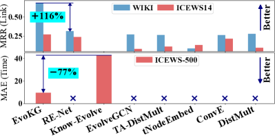
Figure 2. EvoKG wins. EvoKG achieves the best link prediction (top) and time prediction (bottom) results. $\bm{\times}$ indicates that the corresponding method cannot predict event time.

3. Modeling a Temporal Knowledge Graph

We describe how EvoKG models a TKG by addressing the two problems—modeling event time and evolving network structure. The symbols used in this paper are listed in Table 2.

3.1. Modeling Event Time

The temporal patterns of events occurring between various types of entities in a TKG depend on the context of their past interactions. To capture intricate temporal dependencies present in real-world TKGs, we treat the event time $t$ as a random variable, and model the occurrence of triple $(s,r,o)$ at time $t$ using temporal point processes (TPPs), which are the dominant paradigm for modeling events that occur at irregular intervals. Given increasing event times $\{\ldots,t_{n-1},t_{n},\dots\}$, representations in terms of time $t_{n}$ and the corresponding inter-event time $\tau_{n}=t_{n}-t_{n-1}$ are isomorphic, and we use them interchangeably.

Conditional Density Estimation of Event Time. To model the event time, we estimate the conditional probability density $p^{*}_{e}(t)\!=\!p(t|s,r,o,G_{<t})$ of event time $t$, given an event of type $r$ between entities $s$ and $o$, and the history $G_{<t}$ of all past interactions. Note that the star symbol $*$ as in $p^{*}_{e}(t)$ in this paper denotes the dependency on the history $G_{<t}$.

More concretely, in order to define $p^{*}_{e}(t)$, we consider the conditional density of two types of inter-event times $\tau_{\text{eo}}$ and $\tau_{\text{min}}$. Let $p^{*,e}_{\text{{eo}}}(t)=p(\tau_{\text{eo}}|s,r,o,G_{<t})$ be the conditional density of $\tau_{\text{eo}}$, which is the time that has elapsed since entities $s$ and $o$ interacted with each other in their latest event. Also, let $p^{*,e}_{\text{{min}}}(t)=p(\tau_{\text{min}}|s,r,o,G_{<t})$ be the conditional density of $\tau_{\text{min}}$, which is defined to be $\min(\tau_{(s)},\tau_{(o)})$, where $\tau_{(s)}$ and $\tau_{(o)}$ refer to the time that has elapsed since $s$ and $o$ interacted with any other entity in their latest event. In other words, $\tau_{\text{eo}}$ considers how recent the two entities’ interaction was, while $\tau_{\text{min}}$ considers when the most recent event happened in either entity’s history. In experiments where we set $p^{*}_{e}(t)$ to be either of these two probabilities, we find $p^{*,e}_{\text{{min}}}(t)$ and $p^{*,e}_{\text{{eo}}}(t)$ to be most effective for predicting event time (Section 4.2) and temporal links (Section 4.3), respectively. Note that $p^{*}_{e}(t)$ can be more generally defined in terms of both conditional densities to be $p^{*}_{e}(t)=\alpha\cdot p^{*,e}_{\text{{eo}}}(t)+(1-\alpha)\cdot p^{*,e}_{\text{{min}}}(t)$, where $\alpha\,(0\leq\alpha\leq 1)$ weights each term, and it can also be extended with further conditional densities to model different types of inter-event times.

Importantly, our choice to model event time directly via conditional density estimation differs from existing TPP-based approaches for modeling TKGs (Trivedi et al., 2017; Han et al., 2020), where event times are modeled using the conditional intensity function $\lambda^{*}_{e}(t)\!=\!\lambda(t|s,r,o,G_{<t})$, which represents the rate of events happening, given the history. In these intensity-based approaches, computing $p^{*}_{e}(t)$ requires integrating $\lambda^{*}_{e}(t)$, and thus a major challenge lies in selecting a good parametric form for $\lambda^{*}_{e}(t)$. Simple intensity functions (e.g., constant and exponential intensity) have a closed-form log-likelihood, but they usually have limited expressiveness (e.g., they have a unimodal distribution); even if they use RNNs to capture rich temporal information, the resulting distribution $p^{*}_{e}(t)$ still has limited flexibility. More sophisticated ones using neural networks can better capture complex distributions, but their log-likelihood and expectation cannot be obtained in closed form, requiring Monte Carlo approximation. Mixture distributions, on the other hand, are an expressive model for conditional density estimation, with the potential to approximate any density, and with closed-form likelihood and expectation.

Specifically, we use a mixture of log-normal distributions since inter-event times are positive. Log-normal mixture distributions are defined in terms of mixture weights $\bm{w}$, means $\bm{\mu}$, and standard deviations $\bm{\sigma}$. An important consideration in employing a log-normal mixture is that the timing of an event in a TKG is affected by what has happened before (i.e., $G_{<t}$) and what comprises the event triple $e\!=\!(s,r,o)$. In light of this, we obtain the three groups of mixture parameters $\bm{w}_{e}^{*}$, $\bm{\mu}_{e}^{*}$, and $\bm{\sigma}_{e}^{*}\in\mathbb{R}^{K}$, where the symbols $e$ and $*$ signify these parameters’ dependency on the event triple $e$ and the history $G_{<t}$, and $K$ denotes the number of mixture components.

To obtain mixture parameters, we learn entity and relation embeddings such that they reflect their temporal status (which we describe in the next paragraph), as they are influenced by events that occurred over time. Let $\bm{\mathsf{t}}^{*}_{s}$, $\bm{\mathsf{t}}^{*}_{o}$, and $\bm{\mathsf{t}}^{*}_{r}$ denote such temporal embeddings of subject $s$, object $o$, and relation $r$, respectively, after processing events prior to time $t$. We model the conditional dependence of $p(\tau|s,r,o,G_{<t})$ on $e\!=\!(s,r,o)$ and $G_{<t}$ by concatenating the embeddings of $s$, $r$, and $o$ into a context vector $\bm{c}_{e}^{*}=[\bm{\mathsf{t}}^{*}_{s}\|\bm{\mathsf{t}}^{*}_{r}\|\bm{\mathsf{t}}^{*}_{o}]$, and transforming it into the parameters of the log-normal mixture representing $p(\tau|s,r,o,G_{<t})$ using a multilayer perceptron ($\mathrm{MLP}$) as follows:

(3) $$\bm{w}_{e}^{*}=\mathrm{softmax}(\text{$\mathrm{MLP}$}(\bm{c}_{e}^{*})),\bm{\mu}_{e}^{*}=\text{$\mathrm{MLP}$}(\bm{c}_{e}^{*}),\bm{\sigma}_{e}^{*}=\exp(\text{$\mathrm{MLP}$}(\bm{c}_{e}^{*}))$$

where $\mathrm{softmax}$ ensures that mixture weights sum to 1, and $\exp$ makes standard deviations positive. With these parameters, EvoKG defines $p(\tau|s,r,o,G_{<t})$ to be

(4) $$\begin{split}p(\tau|s,r,o,G_{<t})&=p(\tau|\bm{w}_{e}^{*},\bm{\mu}_{e}^{*},\bm{\sigma}_{e}^{*})\\ &=\sum_{k=1}^{K}\frac{(w_{e}^{*})_{k}}{\tau(\sigma_{e}^{*})_{k}\sqrt{2\pi}}\exp\left(-\frac{(\log\tau-(\mu_{e}^{*})_{k})^{2}}{2{(\sigma_{e}^{*})_{k}}^{2}}\right),\end{split}$$

which is a valid probability density function as it is nonnegative and integrates to one for $\tau\in\mathbb{R}_{+}$.

Table 2. Table of symbols.

Symbol Definition $(s,r,o,t)$ directed edge from subject $s$ to object $o$, with edge type (relation) $r$ and timestamp $t$ $e$ event triple $(s,r,o)$ $\tau$ inter-event time (i.e., $\tau_{n}=t_{n}-t_{n-1}$) $\tau_{\text{eo}}$ elapsed time since entities $s$ and $o$ last interacted with each other $\tau_{\text{min}}$ elapsed time since entities $s$ and $o$ last interacted with any other entity $*$ symbol that signifies that an associated symbol (e.g., $p^{*}(\tau)$ and $\bm{\mathsf{t}}^{*}_{i}$) depends on the past events $p^{*}_{e}(\tau)$ conditional probability density function $p(\tau|s,r,o,G_{<t})$ $\bm{w},\bm{\mu},\bm{\sigma}$ weights, means, and standard deviations of a log-normal mixture $\bm{\mathsf{t}}_{i},\bm{\mathsf{s}}_{i},\bm{\mathsf{t}}^{*}_{i},\bm{\mathsf{s}}^{*}_{i}$ temporal (structural) embeddings of entity $i$, with $*$ reflecting its state after processing events until time $t$ $\bm{\mathsf{t}}_{r},\bm{\mathsf{s}}_{r},\bm{\mathsf{t}}^{*}_{r},\bm{\mathsf{s}}^{*}_{r}$ temporal (structural) embeddings of relation $r$, with $*$ reflecting its state after processing events until time $t$ $\bm{\mathsf{t}}_{i}^{(\ell,t)},\bm{\mathsf{s}}_{i}^{(\ell,t)}$ temporal (structural) embeddings of entity $i$ learned by $\ell$-th GNN layer at time $t$ $\bm{\mathsf{t}}_{i}^{(*,t)},\bm{\mathsf{s}}_{i}^{(*,t)}$ temporal (structural) embeddings of entity $i$ updated after events until time $t$ are processed

Time-Evolving Temporal Representations. Informative context for estimating inter-event time can be constructed by summarizing different types of interactions each entity had with others into temporal entity embeddings. Further, how much time elapsed since the latest event gives useful information for learning such temporal representations. To this end, we utilize the neighborhood aggregation framework of relation-aware graph neural networks (GNNs). Specifically, we extend R-GCN (Schlichtkrull et al., 2018) such that the aggregation can take inter-event time $\tau_{i,j}$ between entities $i$ and $j$ into account. Given concurrent events $G_{t}$, we summarize entity $i$’s interaction with others in $G_{t}$ as follows:

(5) $$\bm{\mathsf{t}}_{i}^{(\ell+1,t)}=\sigma\bigg{(}\sum_{r\in\mathcal{R}}\sum_{j\in\mathcal{N}_{t}^{(i,r)}}\frac{1}{\nu_{i,j}}\cdot\bm{\mathbf{{W}}}_{r}^{\ell}\bm{\mathsf{t}}_{j}^{(\ell,t)}+\bm{\mathbf{{W}}}_{0}^{\ell}\bm{\mathsf{t}}_{i}^{(\ell,t)}\bigg{)}$$

where $\bm{\mathsf{t}}_{i}^{(\ell,t)}$ denotes the temporal embeddings of entity $i$ learned by $\ell$-th layer of the extended R-GCN by aggregating events in $G_{t}$; $\nu_{i,j}$ is a factor to consider the inter-event time, which we define to be $\nu_{i,j}=\log\tau_{i,j}$; $\mathcal{R}$ is the set of relations; $\mathcal{N}_{t}^{(i,r)}$ is entity $i$’s concurrent neighbors at time $t$, connected via an edge of type $r$; $\bm{\mathbf{{W}}}_{r}^{\ell}$ and $\bm{\mathbf{{W}}}_{0}^{\ell}$ are the weight matrices in the $\ell$-th layer for relation $r$ and self-loop, respectively. Then with $L$ layers in total, $\bm{\mathsf{t}}_{i}^{L}$ summarizes entity $i$’s temporal interactions in the $L$-hop neighborhood. The initial temporal embeddings $\bm{\mathsf{t}}_{i}^{(0,t)}$ are set to the static representation $\bm{\mathsf{t}}_{i}$ that EvoKG learns to capture the temporal characteristics of entities, i.e., $\bm{\mathsf{t}}_{i}^{(0,t)}=\bm{\mathsf{t}}_{i}$ for any time $t$.

To model the dynamics of temporal updates, the context for modeling inter-event time should reflect the changes made by new events. Given $\bm{\mathsf{t}}_{i}^{(L,t)}$ which summarizes the temporal interaction patterns from concurrent events at time $t$, EvoKG learns time-evolving dynamics from the evolution of $\bm{\mathsf{t}}_{i}^{(L,t)}$ over time, by using recurrent neural networks RNN_te for temporal entity representation learning:

(6) $$\bm{\mathsf{t}}_{i}^{(*,t)}=\textsc{RNN}_{\text{te}}\big{(}\bm{\mathsf{t}}_{i}^{(L,t)},\bm{\mathsf{t}}_{i}^{(*,t-1)}\big{)}$$

where $\bm{\mathsf{t}}_{i}^{(L,t)}$ is the input to RNNs at each time; $\bm{\mathsf{t}}_{i}^{(*,0)}$ is zero-initialized; and $\bm{\mathsf{t}}_{i}^{(*,t)}$ is the temporal embedding of entity $i$ updated after events until time $t$ are processed. In this framework, as aggregating incoming and outgoing neighbors captures sending and receiving patterns between entities, EvoKG aggregates neighborhood in both directions to learn embeddings that reflect different interaction patterns, which are then processed by RNN_te to be used in the context $\bm{c}_{e}^{*}$.

Next, EvoKG considers the concurrent events $G_{t}^{r}$ that have relation $r$, and takes the average of the temporal embeddings of the entities in $G_{t}^{r}$ to provide it as the context $\bm{\mathsf{t}}_{r}^{t}$ to RNN_tr, which learns the temporal embedding $\bm{\mathsf{t}}_{r}^{(*,t)}$ of relation $r$ at time $t$:

(7) $$\bm{\mathsf{t}}_{r}^{(*,t)}=\textsc{RNN}_{\text{tr}}\big{(}\bm{\mathsf{t}}_{r}^{t},\bm{\mathsf{t}}_{r}^{(*,t-1)}\big{)}.$$

For brevity, we use the notation $\bm{\mathsf{t}}_{i}^{*}=\bm{\mathsf{t}}^{(*,t)}_{i}$ and $\bm{\mathsf{t}}_{r}^{*}=\bm{\mathsf{t}}_{r}^{(*,t)}$.

3.2. Modeling Evolving Network Structure

As new events occur, TKGs evolve structurally and the dynamics between entities also change over time. For instance, companies that did not work together may start to collaborate at some point to work on the same project, and this change may influence the communication patterns between them and related entities in the TKG. We capture this intricate structural dynamics by modeling the conditional probability $p(s,r,o|G_{<t})$ of an event triple $(s,r,o)$.

Conditional Density Estimation of Event Triple. To model $p(s,r,o|G_{<t})$, we learn the embeddings of entities and relations (which we discuss in the next paragraph), which capture their time-evolving structural dynamics. For flexibility, we learn these embeddings separately from temporal embeddings discussed in LABEL:{sec:method:temporal}. Let $\bm{\mathsf{s}}_{i}$ and $\bm{\mathsf{s}}_{r}$ denote the static structural embeddings of entity $i$ and relation $r$, and let $\bm{\mathsf{s}}^{*}_{i}$ and $\bm{\mathsf{s}}^{*}_{r}$ be the structural embeddings of entity $i$ and relation $r$ obtained by processing events until time $t$. We concatenate static and dynamic embeddings and denote them using $\mkern 1.5mu\overline{\mkern-1.5mu\bm{\mathsf{s}}\mkern-1.5mu}\mkern 1.5mu^{*}_{i}=[\bm{\mathsf{s}}^{*}_{i}\|\bm{\mathsf{s}}_{i}]$ and $\mkern 1.5mu\overline{\mkern-1.5mu\bm{\mathsf{s}}\mkern-1.5mu}\mkern 1.5mu^{*}_{r}=[\bm{\mathsf{s}}^{*}_{r}\|\bm{\mathsf{s}}_{r}]$. Then EvoKG summarizes the past events $G_{<t}$, which $p(s,r,o|G_{<t})$ is conditioned on, by the graph-level representation $\mkern 1.5mu\overline{\mkern-1.5mu\bm{\mathsf{g}}\mkern-1.5mu}\mkern 1.5mu^{*}$, which EvoKG obtains via an element-wise max pooling over the structural embeddings of all entities, i.e.,

(8) $$\mkern 1.5mu\overline{\mkern-1.5mu\bm{\mathsf{g}}\mkern-1.5mu}\mkern 1.5mu^{*}\!=\!\max(\{\mkern 1.5mu\overline{\mkern-1.5mu\bm{\mathsf{s}}\mkern-1.5mu}\mkern 1.5mu^{*}_{i}\mid i\in\mathrm{entities(}G_{<t}\text{)}\}).$$

Based on these representations, we decompose $p(s,r,o|G_{<t})$ to be

(9) $$p(s,r,o|G_{<t})=p(o|s,r,G_{<t})\cdot p(r|s,G_{<t})\cdot p(s|G_{<t})$$

and parameterize each term separately, as follows:

(10) $$p(o|s,r,G_{<t}) =\mathrm{softmax}\left(\text{$\mathrm{MLP}$}\left([\mkern 1.5mu\overline{\mkern-1.5mu\bm{\mathsf{s}}\mkern-1.5mu}\mkern 1.5mu^{*}_{s}\|\mkern 1.5mu\overline{\mkern-1.5mu\bm{\mathsf{s}}\mkern-1.5mu}\mkern 1.5mu^{*}_{r}\|\mkern 1.5mu\overline{\mkern-1.5mu\bm{\mathsf{g}}\mkern-1.5mu}\mkern 1.5mu^{*}]\right)\right),$$

(11) $$p(r|s,G_{<t}) =\mathrm{softmax}\left(\text{$\mathrm{MLP}$}\left([\mkern 1.5mu\overline{\mkern-1.5mu\bm{\mathsf{s}}\mkern-1.5mu}\mkern 1.5mu^{*}_{s}\|\mkern 1.5mu\overline{\mkern-1.5mu\bm{\mathsf{g}}\mkern-1.5mu}\mkern 1.5mu^{*}]\right)\right),$$

(12) $$p(s|G_{<t}) =\mathrm{softmax}\left(\text{$\mathrm{MLP}$}\left([\mkern 1.5mu\overline{\mkern-1.5mu\bm{\mathsf{g}}\mkern-1.5mu}\mkern 1.5mu^{*}]\right)\right).$$

Time-Evolving Structural Representations. An effective modeling of $p(s,r,o|G_{<t})$ based on the above parameterization depends on learning informative context that reflects how structural dynamics between entities have changed over time. As with learning temporal embeddings, neighborhood aggregation of GNNs and recurrent event modeling using RNNs provide an effective framework to capture this complex structural evolution. Thus, we adapt the framework used for event time modeling in Section 3.1 for learning time-evolving structural embeddings.

Let $\bm{\mathsf{s}}_{i}^{(\ell,t)}$ denote the structural embeddings of entity $i$ learned by $\ell$-th R-GCN layer by aggregating concurrent events $G_{t}$. As before, we set the initial structural embeddings $\bm{\mathsf{s}}_{i}^{(0,t)}$ to $\bm{\mathsf{s}}_{i}$ for each time $t$. Given embeddings $\bm{\mathsf{s}}_{i}^{(\ell,t)}$ for all entities, $\bm{\mathsf{s}}_{i}^{(\ell+1,t)}$ is learned using Equation 5, where $\bm{\mathsf{t}}_{i}^{(\ell,t)}$ is replaced by $\bm{\mathsf{s}}_{i}^{(\ell,t)}$, and $\nu_{i,j}$ is set to the neighborhood size $|\mathcal{N}_{t}^{(i,r)}|$. The structural relation embedding $\bm{\mathsf{s}}_{r}^{t}$ at time $t$ is constructed using concurrent events in the same way as in the temporal case. Then EvoKG learns the time-evolving structural embeddings $\bm{\mathsf{s}}_{i}^{(*,t)}$ and $\bm{\mathsf{s}}_{r}^{(*,t)}$ using RNN_se and RNN_sr as follows.

(13) $$\bm{\mathsf{s}}_{i}^{(*,t)}=\textsc{RNN}_{\text{se}}\big{(}\bm{\mathsf{s}}_{i}^{(L,t)},\bm{\mathsf{s}}_{i}^{(*,t-1)}\big{)},\,\,\bm{\mathsf{s}}_{r}^{(*,t)}=\textsc{RNN}_{\text{sr}}\big{(}\bm{\mathsf{s}}_{r}^{t},\bm{\mathsf{s}}_{r}^{(*,t-1)}\big{)}$$

For brevity, we use the notation $\bm{\mathsf{s}}_{i}^{*}=\bm{\mathsf{s}}^{(*,t)}_{i}$ and $\bm{\mathsf{s}}_{r}^{*}=\bm{\mathsf{s}}_{r}^{(*,t)}$.

3.3. Parameter Learning

Loss Function. Let $\mathcal{L}_{\text{iet}}$ and $\mathcal{L}_{\text{triple}}$ denote the negative log-likelihood (NLL) of the inter-event time and an event triple, respectively. Based on our problem formulation and modeling choices, the two NLLs of a quadruple $q\!=\!(s,r,o,t)$ (i.e., a timestamped event in a TKG) are obtained as follows.

(14) $$\mathcal{L}_{\text{iet}}(q) =-\log p(t|s,r,o,G_{<t})=-\log p(\tau|\bm{w}_{e}^{*},\bm{\mu}_{e}^{*},\bm{\sigma}_{e}^{*})$$

(15) $$\begin{split}\mathcal{L}_{\text{triple}}(q)&=-\log p(s,r,o|G_{<t})\\ &=-\log p(o|s,r,G_{<t})-\log p(r|s,G_{<t})-\log p(s|G_{<t})\end{split}$$

We optimize EvoKG by minimizing the loss $\mathcal{L}$ containing both NLLs for all events in the training set:

(16) $$\mathcal{L} =\sum_{t}\sum_{q=(s,r,o,t)\in G_{t}}\lambda_{1}\,\mathcal{L}_{\text{iet}}(q)+\lambda_{2}\,\mathcal{L}_{\text{triple}}(q)$$

where $\lambda_{1}$ and $\lambda_{2}$ control the importance of each loss term.

Learning Algorithm. Since there exist intricate relational and temporal dependencies among events in TKGs, it is not optimal to decompose events into independent sequences for an efficient training, as we lose relational information. At the same time, since a TKG may cover a long period of time, keeping track of the entire history for each entity can incur prohibitively high computation and memory cost, especially when learning graph-contextualized representations for entities and relations. To address these challenges, we organize events by their timestamps and process concurrent events in parallel, while truncating backpropagation every $b$ time steps (Algorithm 1). As experimental results show, this enables an accurate and efficient parameter learning, which outperforms the best baseline in terms of both prediction accuracy and efficiency.

Input: TKG $G$ with training data, TKG $G^{\prime}$ with validation data, maximum number of epochs $max\_epochs$, number $L$ of R-GCN layers, patience $p$, number of time steps $b$ for truncated backpropagation.

$epoch\leftarrow 1$

repeat

       foreach $t\in\text{Timestamps}(G)$ do

             if $t>0$ then

                   Compute the loss $\mathcal{L}_{t}$ for concurrent events in $G_{t}$ based on Equation 16

                   Optimize model parameters and truncate backpropagation every $b$ time steps

            

            foreach $i\!\in\!\text{Entities}\,(G_{t})$ do /* ​​executed in parallel​​ */

                   Compute $\bm{\mathsf{t}}^{(L,t)}_{i}$ and $\bm{\mathsf{t}}^{*}_{i}$ using eqs. 5 and 6

                   Compute $\bm{\mathsf{s}}^{(L,t)}_{i}$ and $\bm{\mathsf{s}}^{*}_{i}$ using a modified version of eq. 5 and eq. 13

                  

            foreach $r\in\text{Rels}\,(G_{t})$ do /* ​executed in parallel​ */

                   Compute $\bm{\mathsf{t}}^{*}_{r}$ and $\bm{\mathsf{s}}^{*}_{r}$ using eqs. 7 and 13

                  

            

      Evaluate the validation performance for events in $G^{\prime}$

       $epoch\leftarrow epoch+1$

until epoch $=$ max_epochs or no improvement in validation performance for $p$ consecutive times

Algorithm 1 Parameter Learning

Table 3. Statistics of real-world TKGs. Time interval denotes the minimum duration between two temporally adjacent events.

Dataset # Train Edges # Valid Edges # Test Edges # Entities # Rel- ations Time Interval ICEWS18 373,018 45,995 49,545 23,033 256 24 hours ICEWS14 275,367 48,528 341,409 12,498 260 24 hours ICEWS-500 184,725 32,292 228,648 500 256 24 hours GDELT 1,734,399 238,765 305,241 7,691 240 15 minutes WIKI 539,286 67,538 63,110 12,554 24 1 year YAGO 161,540 19,523 20,026 10,623 10 1 year

4. Experiments

In experiments, we answer the following research questions.

• [RQ1] How accurately can EvoKG estimate the event time?

• [RQ2] How accurately can EvoKG predict temporal links?

• [RQ3] How efficient is EvoKG in terms of training and inference?

• [RQ4] How do different parameter settings and event time modeling affect EvoKG’s performance?

After describing the datasets (Section 4.1), we present results for the above research questions (Sections 4.2, 4.3, 4.4 and 4.5). Experimental settings are provided in Appendix A.

4.1. Temporal Knowledge Graph Data

We use five real-world TKGs that have been widely used in previous studies: ICEWS18 (Boschee et al., 2015), ICEWS14 (Trivedi et al., 2017), GDELT (Leetaru and Schrodt, 2013), WIKI (Leblay and Chekol, 2018), and YAGO (Mahdisoltani et al., 2015). ICEWS (Integrated Crisis Early Warning System) and GDELT (Global Database of Events, Language, and Tone) are event-based TKGs; WIKI and YAGO are knowledge bases with temporally associated facts. Statistics of these TKGs are presented in Table 3. We order these datasets by timestamps, and split each one into training, validation, and test sets, as shown in Table 3. We also use ICEWS-500 (Trivedi et al., 2017) for experiments on event time prediction, which is a TKG constructed from ICEWS data, containing a smaller number of nodes than ICEWS18, since some previous studies reported results only on ICEWS-500 without releasing code.

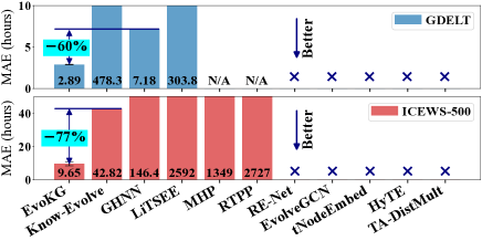
Figure 3. EvoKG achieves the best event time prediction results, with up to 77% less MAE than the second best method; all improvements are statistically significant with $p$-value < 0.05. Note that many methods for TKGs (marked by $\bm{\times}$) cannot predict event time. N/A denotes results are unavailable.

4.2. Event Time Prediction (RQ1)

Task Description. Given an event triple $e\!=\!(s,r,o)$ and the history $G_{<t}$, the goal is to predict when the event $e$ will happen. Specifically, the time of an event triple $e$ is estimated to be the expected value of the time that event $e$ occurs, given the history. Thanks to the use of a mixture distribution, in EvoKG, this expectation is obtained in a closed form by

(17) $$\mathbb{E}_{\tau\sim p^{*}_{e}(\tau)}(\tau)=\sum\nolimits_{k}(w_{e}^{*})_{k}\exp\left((\mu_{e}^{*})_{k}+\nicefrac{{((s_{e}^{*})_{k})^{2}}}{{2}}\right).$$

On the other hand, other approaches, such as GHNN (Han et al., 2020), need to approximate the integral to compute the expected value by using Monte Carlo, as they do not have a close-form solution. We report MAE (mean absolute error), which is the average of the absolute difference between the predicted and true time in hours. Lower MAE indicates higher prediction accuracy.

Baselines. We compare EvoKG against three existing methods for modeling TKGs with the ability to predict event time: Know-Evolve (Trivedi et al., 2017), GHNN (Han et al., 2020), and LiTSEE (Xu et al., 2019). Know-Evolve and GHNN model event time based on temporal point process (TPP) framework. While there exist several other methods for modeling TKGs, they are unable to forecast event time, thus they cannot be used for this evaluation. We also report the result of two other baselines used in (Trivedi et al., 2017), MHP (Multi-dimensional Hawkes Process) and RTPP (Recurrent Temporal Point Process). MHP models dyadic entity interactions as multi-dimensional Hawkes process: an entity pair constitutes an event, and MHP learns when each event occurs, without taking relations (event types) into account. RTPP is a simplified version of RMTPP (Du et al., 2016), which estimates the conditional intensity function of an event by using a global RNN. Relations are also considered in RTPP.

Results. Figure 3 reports the event time prediction accuracy on ICEWS-500 and GDELT . Results of Know-Evolve, RTPP, and MHP are obtained from (Trivedi et al., 2017) (except that we obtained Know-Evolve’s result on GDELT using the reference implementation), and those of LiTSEE and GHNN are taken from (Han et al., 2020). Notably, most TKG methods in Figure 3 are marked with $\times$ due to their inability to estimate event time. Also, the results of RTPP and MHP are not available (marked with ‘n/a’) as their implementation is not publicly available. In EvoKG, we used $\tau_{\text{min}}$ to model the inter-event time. In experiments, methods are updated using the observed graph snapshot at each time step to make future predictions.

Results show that EvoKG consistently outperforms all existing approaches, with up to 77% less MAE than the second-best method. We conduct one-sample t-tests and verify that all improvements over baselines are statistically significant with $p$-value < 0.05. Graph-based methods (EvoKG, Know-Evolve, and GHNN), which learn the temporal patterns of events by utilizing information from the neighborhood, perform much better than simpler baselines (RTPP and MHP), which model event time based only on direct interactions between entities. Also, TPP-based Know-Evolve and GHNN outperform LiTSEE, a non-TPP approach which incorporates time information by adding a temporal component into entity embeddings. EvoKG achieves the best event time prediction results by modeling event time using mixture distributions, which are much more flexible and expressive than those used by existing methods.

4.3. Temporal Link Prediction (RQ2)

Task Description. Given a test quadruple $q\!=\!(s,r,o,t)$ and the history $G_{<t}$, we create a perturbed quadruple $q^{\prime}\!=\!(s,r,o^{\prime},t)$ by replacing $o$ with every other entity $o^{\prime}$ in the graph, and compute the score of $q^{\prime}$. We then sort all perturbed quadruples in descending order of the score and report the rank of the ground truth quadruple $q$. We report MRR (mean reciprocal rank), which is the average of the reciprocal of the ground truth $q$’s rank, and Hits@{3,10}, which is the percentage of correct entities in the top 3 and 10 predictions. For both metrics, higher values indicate better link prediction results.

Baselines. We compare EvoKG against the following baselines for both static and temporal KG reasoning. (1) DistMult (Yang et al., 2015), R-GCN (Schlichtkrull et al., 2018), ConvE (Dettmers et al., 2018), and RotatE (Sun et al., 2019) are methods for static KG reasoning. They are applied to a static, cumulative graph constructed from events in the training data, where edge timestamps are ignored. (2) TA-DistMult (García-Durán et al., 2018) and HyTE (Dasgupta et al., 2018) are methods for temporal KG reasoning in an interpolation setting. (3) dyngraph2vecAE (Goyal et al., 2020), tNodeEmbed (Singer et al., 2019), EvolveGCN (Pareja et al., 2020), and GCRN (Seo et al., 2018) are methods for reasoning over homogeneous graphs in an extrapolation setting. (4) Know-Evolve (Trivedi et al., 2017), DyRep (Trivedi et al., 2019), and RE-Net (Jin et al., 2020) are methods for temporal KG reasoning in an extrapolation setting. GHNN (Han et al., 2020) is not included as the implementation is not available. Also, results reported in (Han et al., 2020) were obtained after applying its own filtering criteria, where GHNN achieved similar results to RE-Net.

Results. Table 4 provides link prediction results on five TKGs. Results of baselines are obtained from (Jin et al., 2020). In EvoKG, we used $\tau_{\text{eo}}$ to model the inter-event time. In experiments, after making predictions at each time step, methods are updated using the observed graph snapshot. EvoKG outperforms all existing approaches across different datasets, achieving up to 116% higher MRR than the best baseline, except on GDELT, where EvoKG achieves similar performance to the best baseline. It is noteworthy that an improvement over baselines is the most significant on WIKI and YAGO, which contains much more events occurring at relatively regular intervals. By modeling event time, EvoKG can predict such temporal patterns accurately. Among baselines, static methods in the first four rows perform worse than the best temporal baseline, RE-Net, as they do not consider temporal factors. At the same time, some temporal methods, such as dyngraph2vecAE and EvolveGCN, often perform worse than static methods, even though they are designed to take temporal evolution of dynamic networks into account. This indicates that incorporating temporal factors needs to be done carefully to avoid introducing additional noise. Know-Evolve and DyRep are the two existing methods based on temporal point processes. While they can be used for temporal link prediction, they are not effective for predicting links, even after applying an MLP decoder to their embeddings, as they focus on modeling just $p(t|s,r,o,G_{<t})$, and thus do not explicitly learn the evolving network structure by modeling $p(s,r,o|G_{<t})$ as in EvoKG. By modeling event time and network structure simultaneously, EvoKG outperforms various existing methods in predicting temporal links and event times.

Table 4. EvoKG outperforms existing methods in terms of temporal link prediction in most cases, achieving up to 116% higher MRR (mean reciprocal rank) on real-world TKGs. Best results are in bold, and second best results are underlined.

Method ICEWS14 ICEWS18 WIKI YAGO GDELT MRR H@3 H@10 MRR H@3 H@10 MRR H@3 H@10 MRR H@3 H@10 MRR H@3 H@10 Static DistMult 9.72 10.09 22.53 13.86 15.22 31.26 27.96 32.45 39.51 44.05 49.70 59.94 8.61 8.27 17.04 R-GCN 15.03 16.12 31.47 15.05 16.49 29.00 13.96 15.75 22.05 27.43 31.24 44.75 12.17 12.37 20.63 ConvE 21.64 23.16 38.37 22.56 25.41 41.67 26.41 30.36 39.41 41.31 47.10 59.67 18.43 19.57 32.25 RotateE 9.79 9.37 22.24 11.63 12.31 28.03 26.08 31.63 38.51 42.08 46.77 59.39 3.62 2.26 8.37 Temporal TA-DistMult 11.29 11.60 23.71 15.62 17.09 32.21 26.44 31.36 38.97 44.98 50.64 61.11 10.34 10.44 21.63 HyTE 7.72 7.94 20.16 7.41 7.33 16.01 25.40 29.16 37.54 14.42 39.73 46.98 6.69 7.57 19.06 dyngraph2vecAE 6.95 8.17 12.18 1.36 1.54 1.61 2.67 2.75 3.00 0.81 0.74 0.76 4.53 1.87 1.87 tNodeEmbed 13.36 13.13 24.31 7.21 7.64 15.75 8.86 10.11 16.36 3.82 3.88 8.07 12.97 12.61 21.22 EvolveGCN 8.32 7.64 18.81 10.31 10.52 23.65 27.19 31.35 38.13 40.50 45.78 55.29 6.54 5.64 15.22 Know-Evolve 0.05 0.00 0.10 0.11 0.00 0.47 0.03 0.00 0.04 0.02 0.00 0.01 0.11 0.02 0.10 Know-Evolve+MLP 16.81 18.63 29.20 7.41 7.87 14.76 10.54 13.08 20.21 5.23 5.63 10.23 15.88 15.69 22.28 DyRep+MLP 17.54 19.87 30.34 7.82 7.73 16.33 10.41 12.06 20.93 4.98 5.54 10.19 16.25 16.45 23.86 R-GCRN+MLP 21.39 23.60 38.96 23.46 26.62 41.96 28.68 31.44 38.58 43.71 48.53 56.98 18.63 19.80 32.42 RE-Net 23.91   26.63   42.70   26.81   30.58   45.92   31.55   34.45   42.26   46.37   51.95   61.59   19.44 20.73 33.81     EvoKG 27.18 $\pm$0.001 30.84 $\pm$0.001 47.67 $\pm$0.001 29.28 $\pm$0.002 33.94 $\pm$0.004 50.09 $\pm$0.002 68.03 $\pm$0.031 79.60 $\pm$0.036 85.91 $\pm$0.063 68.59 $\pm$0.003 81.13 $\pm$0.005 92.73 $\pm$0.009 19.28   $\pm$0.001 20.55   $\pm$0.001 34.44 $\pm$0.002  

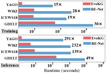
Figure 4. EvoKG performs training (top) and inference (bottom) up to $30\times$ and $291\times$ faster than RE-Net.

4.4. Efficiency (RQ3)

Setup. We compare EvoKG against RE-Net, the best performing baseline method for temporal link prediction, in terms of model training and inference speed. We evaluate the training speed by measuring the time taken to train one epoch, and the inference speed by measuring the time taken to evaluate the entire test data in terms of $p(s,r,o|G_{<t})$.

Results. Figure 4 shows the time taken for training (top) and inference (bottom) over four TKGs. The training speed for EvoKG is 23$\times$ on average, and up to 30$\times$, faster than RE-Net. In making inferences, EvoKG is 177$\times$ on average, and up to 291$\times$, faster than RE-Net. This is because RE-Net’s design for handling events results in a lot of repeated computations for neighborhood aggregation and processing event history. The difference in runtime is even more pronounced in making inferences since RE-Net processes event quadruples individually during inference. On the other hand, EvoKG processes concurrent events simultaneously, effectively reducing redundant operations. As a result, EvoKG performs both tasks much more efficiently than RE-Net.

4.5. Ablation Study (RQ4)

4.5.1. Parameter Sensitivity

We evaluate how the performance of EvoKG changes, as we vary (a) the embedding size, (b) the number of R-GCN layers, (c) the number of mixture components, and (d) truncation length (the number of time steps between backpropagation truncation in RNNs). Figure 5 shows the link prediction result on ICEWS18 (top), and event time prediction result on ICEWS-500 (bottom); reported values denote the ratio of the result obtained with the parameter setting on the x-axis to the best result.

Embedding Size. We set the embedding size (both temporal and structural embeddings) to 100, 200, and 400. As Figures 5(a) and 5(b) show, the best accuracy on the two datasets is achieved by an embedding size of 100, while using a much larger embedding size of 400 hurts the performance, as this leads to overfitting.

Number of R-GCN Layers. EvoKG extends R-GCNs for learning temporal and structural representations. The number of R-GCN layers determines the size of the neighborhood from which a node aggregates information. For predicting both temporal link and event time, using two layers leads to a better result than using a single layer, indicating that an increased neighborhood brings useful information for modeling a TKG. However, using more layers can incur over-smoothing issues, decreasing time prediction accuracy.

Number of Mixture Components. EvoKG uses a mixture distribution to model the event time. The number of mixture components affects the flexibility of the mixture distribution. Figures 5(a) and 5(b) report the performance of EvoKG as the number of mixtures is set to 16, 64, 128, and 256. EvoKG achieves the best link and event time prediction results, with 16 and 64 mixture components, respectively. While using a larger number of mixture components decreases performance, EvoKG still achieves high accuracy, and is not very sensitive to these parameter settings.

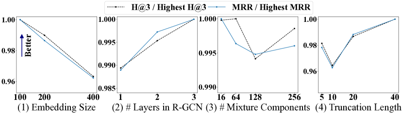
(a) Temporal link prediction performance of EvoKG on ICEWS18.

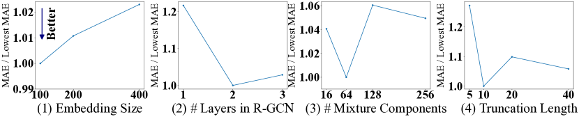
(b) Event time prediction performance of EvoKG on ICEWS-500.

Figure 5. Link prediction and event time prediction performance as we vary (1) embedding size, (2) number of R-GCN layers, (3) number of mixture components, and (4) truncation length.

Truncation Length. For efficient and scalable training, EvoKG truncates backpropagation every $b$ time steps (Algorithm 1). We set $b$ to 5, 10, 20, and 40, and measure the performance. On the two datasets, the best result is achieved with $b=40$ (link prediction) and $b=10$ (event time prediction), and using a smaller time steps tends to decrease the accuracy, as this restricts the model’s ability to keep track of the history. Results also show that if the truncation length is longer than appropriate, it may hurt the predictive accuracy.

4.5.2. Effects of Event Time Modeling

To evaluate the importance of modeling event time in the overall quality of TKG modeling, we report in Figure 6 the improvement made by event time modeling in terms of link prediction accuracy on all TKGs. Specifically, let $\text{Acc}_{\text{1,2}}$ and $\text{Acc}_{\text{2}}$ be the link prediction performance obtained with both terms and only the second term in Equation 2, respectively. The improvement in Figure 6 is defined to be $((\text{Acc}_{\text{1,2}}-\text{Acc}_{\text{2}})/\text{Acc}_{\text{2}})\times 100$. Results show that modeling event time consistently improves the prediction accuracy on all datasets, by up to 61%.

5. Related Work

In this section, we review previous works on reasoning over graphs.

Reasoning over Static Graphs. Inspired by the success of the Skip-gram model (Mikolov et al., 2013) in NLP, several methods (Grover and Leskovec, 2016; Perozzi et al., 2014; Tang et al., 2015) learn node embeddings that maximize the likelihood of preserving neighborhoods of nodes in a network via random walks. More recently, many graph neural networks (GNNs) have been developed for representation learning in homogeneous graphs for semi-supervised and self-supervised settings, including GCN (Kipf and Welling, 2017) and GAT (Velickovic et al., 2018).

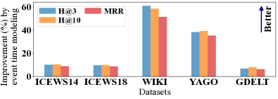
Figure 6. Modeling event time improves temporal link prediction accuracy on all TKGs, by up to 61%.

To learn the representations of entities and relations in heterogeneous KGs, tensor factorization (TF) (Kolda and Bader, 2009) has been widely used. There exist several types of TF methods (Park et al., 2016, 2019; Oh et al., 2019; Jeon et al., 2016; Gujral et al., 2020), such as CP and Tucker decomposition, which make different assumptions on the underlying data generating process. Yet, most TF methods are not well suited for temporal data (e.g., they do not take inter arrival times into account). In recent years, various relational learning techniques have been proposed for heterogeneous KGs, using different scoring functions to evaluate the triples in KGs, including models with distance-based scoring functions (e.g., TransE (Bordes et al., 2013), RotatE (Sun et al., 2019)) and models based on semantic matching (e.g., RESCAL (Nickel et al., 2011), DistMult (Yang et al., 2015), NTN (Socher et al., 2013), ConvE (Dettmers et al., 2018)). GNNs have also been extended for relation-aware representation learning on KGs, such as R-GCN (Schlichtkrull et al., 2018) and HAN (Wang et al., 2019). Overall, these methods are developed for static graphs and lack the ability to model temporally evolving dynamics.

Reasoning over Dynamic Homogeneous Graphs. To capture temporal dynamics in time-evolving graphs, RNNs have been used to summarize and maintain evolving entity states in many methods (Seo et al., 2018; Rossi et al., 2020; Pareja et al., 2020; Kumar et al., 2019; Singer et al., 2019). Often, GNNs have been combined with RNNs to capture both structural and temporal dependencies (Seo et al., 2018; Rossi et al., 2020; Pareja et al., 2020). Another line of work (Xu et al., 2020; Sankar et al., 2020) employed graph attention mechanisms to make the model aware of the temporal order and the time span between entities when computing the attention weights. Some other approaches applied deep autoencoders to dynamic graph snapshots (Goyal et al., 2018, 2020), enforced temporal smoothness on entity embeddings (Zhu et al., 2016; Zhou et al., 2018), and performed temporal random walks (Nguyen et al., 2018). As these methods are designed for single-relational dynamic graphs, they lack mechanisms to capture the multi-relational nature of TKGs, which we focus on in this paper.

Reasoning over Dynamic Heterogeneous Graphs. Static KG embedding methods have been extended to take temporal information into account, including TA-DistMult (García-Durán et al., 2018), TTransE (Leblay and Chekol, 2018), HyTE (Dasgupta et al., 2018), and diachronic embedding (Goel et al., 2020). These temporal KG embedding techniques address an interpolation problem where the goal is to infer missing facts at some point in the past, and cannot predict future events. Recently, several methods have been developed to tackle the extrapolation problem setting, where the goal is to predict new facts at future time steps. TensorCast (de Araujo et al., 2017) uses exponential smoothing to forecast latent entity representations, obtained with TF. RE-Net (Jin et al., 2020) learns dynamic entity embeddings by summarizing concurrent events in an autoregressive architecture; yet, it has no components to model the event time. Know-Evolve (Trivedi et al., 2017), DyRep (Trivedi et al., 2019), and GHNN (Han et al., 2020) model the occurrences of events over time by using temporal point processes (e.g., Rayleigh and Hawkes processes) that estimate the conditional intensity function. Inspired by (Shchur et al., 2020), EvoKG models the event time by directly estimating its conditional density in a flexible and efficient framework.

In summary, most existing methods for both homogeneous and heterogeneous dynamic graphs model just the second term on the evolving network structure in Equation 2, and thus cannot predict when events will occur. On the other hand, a few methods like (Trivedi et al., 2017, 2019) that model the first term on the evolving temporal patterns in Equation 2 do not model the other term, which greatly limits their reasoning capacity. In this paper, we present a problem formulation that unifies these two major tasks (Section 2), and develop an effective framework EvoKG that tackles them simultaneously.

6. Conclusion

Temporal knowledge graphs (TKGs) represent facts about entities and their relations, which occurred at a specific time, or are valid for a specific duration of time. Reasoning over TKGs, i.e., inferring new facts from TKGs, is crucial to many applications, including question answering and recommender systems. Towards an effective reasoning over TKGs, this paper makes the following contributions.

• Problem Formulation. We present a problem formulation that unifies the two core problems for TKG reasoning—modeling the timing of events and the evolving network structure.

• Framework. We develop EvoKG, an effective framework for modeling TKGs that jointly addresses the two core problems.

• Effectiveness & Efficiency. Experiments show that EvoKG outperforms existing methods in terms of effectiveness (link and time prediction accuracy improved by up to 116%) and efficiency (training speed improved by up to 30$\times$ over the best baseline).

Reproducibility. The code and data are available at https://namyongpark.github.io/evokg.

Future Work. We plan to improve the explainability and transparency of EvoKG, such that EvoKG can answer questions like “When entity $i$ is estimated to interact with entity $j$, which past events had great influence on their current relationship?”. We also plan to extend EvoKG for anomaly detection in dynamic networks.

Appendix A Appendix

A.1. Experimental Settings

Data Split. We split datasets into training, validation, and test sets in chronological order, as shown in Table 3. For training EvoKG, we applied early stopping, checking the validation performance with a patience of five. Then the model with the best validation performance was used for testing.

Hyperparameters. We used a two-layer R-GCN (Schlichtkrull et al., 2018) with block diagonal decomposition (BDD), which reduces the number of parameters and alleviates overfitting, and set the size of entity and relation embeddings in EvoKG to 200 (except for WIKI, where it was set to 192 to meet the constraint of using R-GCN with BDD). Static entity embeddings were initialized using the Glorot initialization, while the initial dynamic embeddings were zero-initialized. We used a single-layer Elman RNN with tanh non-linearity, but different RNNs, such as GRU, can easily be used. We trained the model using the AdamW optimizer with a learning rate of 0.001, a weight decay of 0.00001, $\beta_{1}=0.9$, and $\beta_{2}=0.999$, and applied dropout with $p=0.2$. As training the module for modeling network structure usually takes longer than training the module for modeling event time, we first trained the model with $\lambda_{1}\!=\!0$ and $\lambda_{2}\!=\!1$, and then trained the entire model with $\lambda_{1}\!=\!\lambda_{2}=1$ until convergence. We truncated the backpropagation for RNNs every 40 time steps for GDELT, and every 20 time steps for other datasets. We set the number $K$ of mixture components to 128.

For the details of baselines used in this work, please refer to (Trivedi et al., 2017) for Know-Evolve, RTPP, and MHP; (Han et al., 2020) for GHNN and LiTSEE; and (Jin et al., 2020) for other baselines including RE-Net.

Compute Resources. We ran experiments on a Linux machine with 8 CPUs (Intel(R) Xeon(R) CPU E5-2623 v4 @ 2.60GHz), 30GB RAM, and an NVIDIA Quadro P6000 GPU.

Software. To implement EvoKG and the evaluation pipeline, we used the following software (software version is specified in the parentheses): python (3.8.3), Deep Graph Library (0.53), PyTorch (1.7.1), NumPy (1.18.5), and pandas (1.0.5). We used PyTorch’s RNN implementation, and Deep Graph Library’s R-GCN implementation.