One Configuration to Rule Them All?
Towards Hyperparameter Transfer in Topic Models
using Multi-Objective Bayesian Optimization

Abstract

Topic models are statistical methods that extract underlying topics from document collections. When performing topic modeling, a user usually desires topics that are coherent, diverse between each other, and that constitute good document representations for downstream tasks (e.g. document classification). In this paper, we conduct a multi-objective hyperparameter optimization of three well-known topic models. The obtained results reveal the conflicting nature of different objectives and that the training corpus characteristics are crucial for the hyperparameter selection, suggesting that it is possible to transfer the optimal hyperparameter configurations between datasets.

1 Introduction

Topic models Blei (2012) are statistical methods that extract the underlying themes (“topics”) from a document corpus. Topics are often represented by sets of words that make sense together, e.g. the words “cat, animal, dog, mouse” may represent a topic about animals. Topic models’ evaluations are usually limited to the comparison of models whose hyperparameters are fixed Doan and Hoang (2021). However, hyperparameters can affect models’ performance and fixing them prevents the researchers from discovering the best topic model on a dataset.

Terragni et al. (2021) proposed a first attempt to conduct a robust comparison between models, using single-objective hyperparameter optimization to automatically get the optimal hyperparameters. This has been later extended to multi-objective hyperparameter optimization Terragni and Fersini (2021). Yet, they do not provide a thorough and extensive experimentation using either single or multi-objective optimization, which may reveal possibly competing objectives.

In fact, topic models can be evaluated in several ways: from downstream tasks, such as document classification and information retrieval Boyd-Graber et al. (2017), to the analysis of the generated topics Lau et al. (2014); Chang et al. (2009). However, previous work Nan et al. (2019) noted that these objectives can be conflicting. For example, a topic model that produces good document representations may not be able to produce coherent and diverse topics simultaneously.

To this purpose, we further explore this direction by using the Multi-Objective Bayesian Optimization (MOBO) Paria et al. (2019) approach to optimize the hyperparameters of three well-known topic models according to three criteria: topic coherence, topic diversity, and document classification. Exploring the space of the hyperparameters using MOBO leads to jointly discover the best models according to the three considered objectives and reveal the conflicting nature of different objectives.

Moreover, we investigate whether the discovered best hyperparameter configurations are consistent across datasets having different characteristics. In other words, we verify if we can always transfer the optimal configuration of hyperparameters from a dataset to another one, or if the dataset features play a part in the hyperparameter transfer problem.

Contributions.

In this paper, we show that we can use MOBO to boost the performance of topic models according to multiple objectives. However, these objectives are often competing (Research Statement RS #1), leading to a model that is excellent for a purpose but performs poorly for another objective. Thus, a user would need to find a balance between different and conflicting objectives.

Our results also show that, in some cases, we can transfer the best hyperparameter configurations from a dataset to an unseen dataset (Research Statement RS #2). This result suggests that we need to take into consideration the dataset features when performing the hyperparameter transfer.

2 Related Work

Hyperparameter Optimization.

Researchers adopt different strategies to address the problem of hyperparameters selection for topic models. They usually select a priori values according to domain knowledge. Yet, in most cases, there is no knowledge of the topic distribution over the corpus. An alternative is to select the hyperparameter configuration using grid search techniques Griffiths and Steyvers (2004); Pavlinek and Podgorelec (2017). Grid search is simple and parallelizable but suffers from the curse of dimensionality, as the number of possible configurations grows exponentially with the number of hyperparameters and the range of possible values Bergstra and Bengio (2012).

Another option adopts fixed-point methods for estimating the hyperparameters of a model Wallach (2008); Asuncion et al. (2009). The inference algorithm alternates between sampling the topics and inferring the hyperparameters. Terragni et al. (2021) recently proposed OCTIS, a topic modeling framework which incorporates a black-box optimization approach, i.e. Bayesian Optimization, to optimize the hyperparameters of topic models. Bayesian techniques can be superior to point estimates and grid search techniques Snoek et al. (2012). However, a single-objective strategy disregards the importance of the other objectives in topic models. Indeed, this work has been later extended to Multi-Objective optimization Terragni and Fersini (2021), although in both works an extensive experimental campaign is missing.

Multi-objective topic modeling.

Although the literature on topic modeling evaluation is rich and diverse Chang et al. (2009); Korencic et al. (2018); Wallach et al. (2009), only a few efforts have been made to tackle this task as a multi-objective optimization problem. Khalifa et al. (2013) and González-Santos et al. (2021) investigate the use of multi-objective evolutionary algorithms for topic modeling to infer coherent topics by searching trade-offs with regards to three objectives: topic coverage, topic coherence, and perplexity. Other approaches Vorontsov and Potapenko (2015); Ding et al. (2018); Veselova and Vorontsov (2020) explicitly model additional objectives into the process of building the topic model, e.g. by adding extra terms to the optimization objective/loss function.

Our approach differs from the previously presented methods because it is model-agnostic. Moreover, we use hyperparameter optimization aiming to show that we need to compromise between different conflicting metrics and it is possible to zero-shot transfer the best hyperparameter configurations to unseen datasets.

3 Multi-objective Optimization for Topic Models

To investigate the role of multi-objective optimization in topic models, we optimize the topic models’ hyperparameters by adopting a Bayesian Optimization (BO) strategy Mockus et al. (1978); Archetti and Candelieri (2019); Kandasamy et al. (2020); Paria et al. (2019). BO is a Sequential Model-Based Optimization strategy that allows us to optimize the hyperparameters of a model requiring little prior knowledge. In a single-objective setting, BO uses the model’s configurations evaluated so far to approximate the value of the objective performance metric with respect to the model’s hyperparameters and then selects a new promising configuration to evaluate. BO is based on two key components: a probabilistic surrogate model aiming at approximating the performance metrics to optimize and an acquisition function (also named utility function or infill criterion) to select the next configuration.

Single-objective BO can be generalized to multiple objective functions Paria et al. (2019), where the final aim is to recover the Pareto frontier of the objective functions, i.e. the set of Pareto optimal points. A point is Pareto optimal if it cannot be improved in any of the objectives without degrading some other objective. In this paper, we will use the multi-objective methodology presented in Paria et al.. We refer the readers to Paria et al. (2019) for additional details on multi-objective Bayesian optimization and to Terragni et al. (2021); Terragni and Fersini (2021) to the use of hyperaparameter Bayesian Optimization in topic modeling.

Objective functions.

We consider three well-known objective functions that investigate different aspects of a topic model: the quality of the topics, the diversity of the topics, and the prediction capability of the model in a classification task. These three aspects are usually investigated in the topic modeling literature Chang et al. (2009); Dieng et al. (2020); Terragni et al. (2020). All the considered functions must be maximized.

• Topic Coherence measures how much the top-$n$ words representing each topic are related. A well-known metric of topic coherence is NPMI Lau et al. (2014), which is computed using Normalized Pointwise Mutual Information of each pair of words $(w_{i},w_{j})$ in the top-10 words of each topic.

• Topic diversity measures how much the top-$n$ words of a topic differ from another topic. We use a recent metric Bianchi et al. (2021a) based on Ranked-Biased Overlap Webber et al. (2010). Topics with common words at different rankings are penalized less than topics sharing the same words at the highest ranks. We will refer to this metric as IRBO.

• The predicting capability refers to the capability of a topic model to produce a good document representation. The topic distribution of each document is used to train a classifier. Here, we use a polynomial SVM and we compute the Micro-F1 measure, i.e. the weighted average of the F1 measure for each class (each dataset has a number of classes, specified in Table 1). We will refer to this metric as F1.

4 Hyperparameter Transfer

The knowledge related to optimal hyperparameter configurations, which we acquire during the multi-objective optimization, can be transferred to an unseen dataset. We follow a simple and effective hyperparameter transfer approach, based on the work of Feurer et al. (2014).

Let $f_{i}(x)$ with $i=\{1,\ldots,N\}$ denote an objective function (here, $N=3$) and $\theta_{i}^{1},\ldots,\theta_{i}^{D}$ denote the best hyperparameter configurations discovered by MOBO for the previously seen datasets $1,\ldots,D$ respectively. Each $\theta_{i}^{d}$ is composed of the $t$ best hyperparameters configuration for the objective function $f_{i}$. In Feurer et al., the authors define some dataset features, also called metafeatures, and a similarity measure for each feature, thus allowing to initialize the surrogate model of the BO with best hyperparameter configurations of the dataset that is the most similar.

In this paper, we follow an opposite direction to see if an optimal hyperparameter configuration is consistent across different datasets (RS #2). We train a topic model on an unseen target dataset with the best hyperparameter configurations $\theta_{i}^{d}$ of previously seen dataset $d$ for the given objective function $f_{i}$. If a configuration can be effectively transferred to every dataset (i.e. the best hyperparameter configuration transferred from a dataset to the target one and vice versa achieves performances that are close to the optimal ones), then it follows that the configurations are independent of the datasets’ features. Otherwise, if some configurations do not transfer well on a target dataset, it implies that the hyperparameter configurations are dependent on the metafeatures.

5 Experimental Setting

5.1 Models

In our evaluation, we consider three distinct topic models, chosen to be the representatives of different categories of topic models Stevens et al. (2012); Zhao et al. (2021): classical probabilistic models, matrix factorization methods, and neural topic models. Due to their different formulations, all the considered models are controlled by different types of hyperparameters that we will detail in Section 5.5.

LDA

(Blei et al., 2003, Latent Dirichlet Allocation) is a generative probabilistic model that describes a corpus of documents through a set of topics $K$, seen as distributions of words over a vocabulary $W$. A document is assumed composed of a mixture of different topics that follow a Dirichlet distribution, where a topic drawn from this mixture is assigned to each word of the document.

NMF

(Paatero and Tapper, 1994, Non-Negative Matrix Factorization) is a statistical method that reduces the dimensionality of the input corpus of $D$ documents, viewed as a matrix $M$ of shape $D\times|W|$, where $|W|$ represents the length of the vocabulary. It aims at decomposing $M$ as the product of two matrices $V$ and $H$, such that the dimension of $V$ is $|W|\times K$ and that of $H$ is $D\times K$. The decomposed matrices must consist of only non-negative values.

CTM

(Zero-shot Contextualized Topic Model) Bianchi et al. (2021b) is a recent neural topic model, based on the Variational Autoencoder (VAE) architecture. The neural variational framework trains a neural inference network to directly map a contextualized document representation – e.g. coming from BERT Devlin et al. (2019)– into a continuous $K$-dimensional latent representation. Then, a decoder network reconstructs the document Bag-of-Word representation by generating its words from the latent document representation.

5.2 Datasets

We consider 6 different datasets: 20 NewsGroups (20NG), AFP, BBC News (BBC) Greene and Cunningham (2006), M10 Lim and Buntine (2014), StackOverflow (SO), and SearchSnippets (SS) Phan et al. (2008). Moreover, the AFP dataset is in French, while the others are in English. We report the main statistics of the preprocessed datasets in Table 1 and the preprocessing details in the Appendix. The datasets are split in training (70%), testing (15%) and validation set (15%).

Name	# Docs	# Labels	# Unique words	Avg doc length (std)
20NG	16,309	20	1612	48 (130)
AFP	26,599	17	2686	156 (174)
BBC	2,225	5	2949	120 (72)
M10	8,355	10	1696	6 (2)
SS	12,295	8	4705	14 (5)
SO	16,407	20	2257	5 (2)

Table 1: Characteristics of the studied datasets

5.3 Multi-objective Hyperparameter Optimization

To simultaneously optimize topic quality (NPMI), topic diversity (IRBO) and classification (F1), we use the Dragonfly library Kandasamy et al. (2020); Paria et al. (2019) integrated into the topic modeling framework OCTIS Terragni et al. (2021); Terragni and Fersini (2021). To obtain robust evaluations, we train each model 30 times and consider the median of the 30 evaluations as the evaluation of the function to be optimized. A number $n$ of initial configurations is randomly sampled via Latin Hypercube Sampling ($n$ equal to the number of hyperparameters to optimize plus 2 to provide enough configurations for the initial surrogate model to fit). The total number of BO iterations for each model is 125. We use Gaussian Process as the probabilistic surrogate model and the Upper Confidence Bound (UCB) as the acquisition function.

5.4 Single-objective Hyperparameter Optimization

Similarly to 5.3, we use the Dragonfly to perform single-objective Bayesian Optimization to optimize each of the individual metrics, to compare the performance on individual metrics when switching to the MO setting. Again, we use the same number of iterations and hyperparameters search space.

5.5 Hyperparameter setting

Model	Hyperparameter	Values/Range
All	Number of topics	[5, 150]
LDA	$\alpha$ prior	[$10^{-4},10$]
	$\beta$ prior	[$10^{-4},10$]
NMF	Regularization factor	[0, 0.5]
	L1-L2 ratio	[0,1]
	Initialization method	random, nndsvd, nndsvda, nndsvdar
	Regularization	V matrix, H matrix, both
CTM	Activation function	softplus, relu, sigmoid, leakyrelu, rrelu, elu, selu
	Dropout	[0, 0.95]
	Learn priors	true (1), false (0)
	Learning rate	[$10^{-4},10^{-1}$]
	Momentum	[0, 0.9]
	Number of layers	1, 2, 3, 4, 5
	Number of neurons	100, 200, 300, 400, 500, 600, 700, 800, 900, 1000
	Optimizer	adagrad, adam, sgd, adadelta, rmsprop

Table 2: Hyperparameters and ranges.

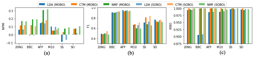
Figure 1: Best performance of the topic models for each evaluation metric on the considered datasets: (a) NPMI, (b) F1 (c) IRBO.

We summarize the models’ hyperparameters and their corresponding ranges in Table 2. For each model, we optimize the number of topics, ranging from 5 to 150 topics. Regarding LDA, we also optimize the hyperparameters $\alpha$ and $\beta$ priors that the sparsity of the topics in the documents and sparsity of the words in the topic distributions respectively. These hyperparameters are set to range between $10^{-4}$ and $10$ on a logarithmic scale.

The hyperparameters of NMF are mainly related to the regularization that can be applied to the factorized matrices. The regularization hyperparameter controls if the regularization is applied only to the matrix $V$, or to the matrix $H$, or both of them. The regularization factor is the constant that multiplies the regularization terms. It ranges between 0 and 0.5 (where 0 means no regularization). L1-L2 ratio controls the ratio between L1 and L2-regularization. It ranges between 0 and 1, where 0 corresponds to L2 only, 1 corresponds to L1 only, otherwise it is a combination of the two types. We also optimize the initialization method for the matrices $W$ and $H$.

Since CTM is a neural topic model, its hyperparameters are mainly related to the network architecture. We optimize the number of layers (ranging from 1 to 5), and the number of neurons (ranging from 100 to 1000, with a step of 100). For simplicity, each layer has the same number of neurons. We also consider different variants of activation functions and optimizers. We set the dropout to range between 0 and 0.95 and the momentum between 0 and 0.9. Finally, we optimize the learning rate, that is set to range between $10^{-4}$ and $10^{-1}$, on a logarithm scale, and the hyperparameter learn priors that controls if the priors are learnable parameters. We fix the batch size to 200 and we adopted an early stopping criterion for determining the convergence of each model. Following Bianchi et al. (2021b), we use the contextualized document representations derived from SentenceBERT Reimers and Gurevych (2019). In particular, we use the pre-trained RoBERTa model fine-tuned on STS for the English datasets and the multilingual Universal Sentence Encoder for AFP.

For all the models, we set the remaining parameters to their default values. The models, metrics and the SOBO and MOBO pipelines are integrated into the open-source topic modeling framework OCTIS Terragni et al. (2021); Terragni and Fersini (2021).

5.6 Hyperparameter Transfer Setting

Regarding the hyperparameter transfer task, we consider the 5 best hyperparameter configurations for each metric, model, and dataset obtained during the multi-objective optimization experiments. We use the identified evaluations coming from a dataset to train a topic model on a different target dataset. As before, to obtain a robust result, we train the model with the same hyperparameter configuration 30 times and consider the median of the 30 evaluations.

6 Results

In the following, we discuss the results of the MOBO experiments and the hyperparameter transfer experiments. We report the best 5 hyperparameter configuration for each model and metric on each dataset in the Appendix.

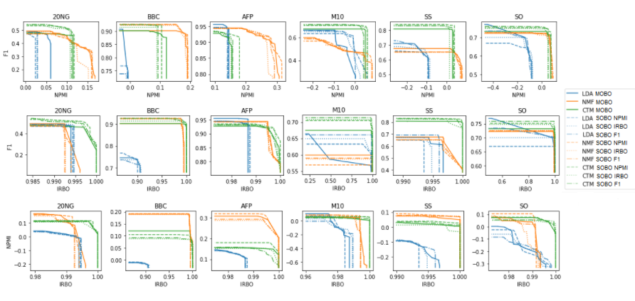
Figure 2: Pareto frontier for each pair of metrics on the considered datasets.

6.1 Multi-objective hyperparameter optimization (RS #1)

No topic model wins them all.

Figure 1 reports the best performance of the models for each metric and dataset obtained by the MOBO experiments. It is important to notice that the hyperparameter configuration that allows a topic model to obtain the best performance for a given metric may differ from the optimal hyperparameter configuration for another evaluation metric.

Regarding the models’ performance for the topic coherence (subfigure  1.a), we can observe that NMF outperforms the other models in most cases. The stronger regularization in NMF generally leads to sparse topics and this likely leads to higher coherence scores Burkhardt and Kramer (2019). Considering the predicting capabilities of the models (subfigure  1.b), CTM usually outperforms LDA and NMF for short-text documents (M10, SS), while LDA gets the best results in long-text datasets (20NG, BBC, AFP). We note that CTM incorporates contextualized representations originated by a limited number of tokens, and not by the entire document. It follows that the representations of CTM may not produce accurate results for long-text documents. Finally, in the subfigure  1. c, we observe that CTM and NMF reach comparable topic diversity performance, often getting topics that are totally different from each other.

On the same figure, we see the performance of the same models obtained by SOBO on each dataset. At first glance, we can see that for most combinations of dataset and metric, the MO models perform on par with their SO counterparts, suggesting that even under the multi-objective constraint, not much is sacrificed in performance on individual metrics (while improving the performance on the other metrics).

As a concluding remark, except for the coherence, we showed that it is difficult to determine an always-winning topic model when we boost the performance of the models using multi-objective optimization. This finding is consistent with other investigations Stevens et al. (2012); Korencic et al. (2018), despite that previous work did not optimize the models’ hyperparameters. This result raises a question on the fairness of the past comparisons between topic models. This contributes to the growing amount of negative results when reviewing previously published work in light of new experiments Rogers et al. (2020).

Conflicting objectives.

Although considering the best performance for each topic model can provide an indicator of its capabilities, it is essential not to focus on a single metric, but rather to jointly consider multiple objectives. Hereby, we show the trade-off between a pair of metrics by plotting the Pareto frontier of the considered metrics. Figure 2 shows the frontier of each model for the pairs of metrics (NPMI, IRBO), (F1, NPMI) and (F1, IRBO) respectively.

We can observe that in most cases no model dominates the others, i.e. there is not any Pareto frontier that is better than the others for all the objectives. For example, if we consider the frontiers for NPMI and IRBO on 20NG, the frontier of the models CTM and NMF dominates LDA. However, CTM and NMF do not dominate each other. In other words, for the dataset 20NG, a user that aims at obtaining coherent and diverse topics has to compromise between the two objectives.

In some cases, a topic model that outperforms the others for a given metric performs very poorly considering other metrics. For example, LDA on M10 obtains the best topic coherence but achieves a very low F1 (<0.2). Specifically, when considering F1 vs NPMI, we observe that to obtain high performance for a given metric we need to degrade the others, and vice versa.

On the same figures, we can compare again this performance in between the single-objective and multi-objective. On most datasets, the MOBO models perform better than their SOBO counterparts. On the remaining datasets, we can see that the SOBO can perform better on singular metric it’s trained on, thus pushing its Pareto frontier beyond that of its MOBO counterpart.

These results enforce the idea of not limiting the experimental campaign of topic models to a single-objective hyperparameter optimization approach. This approach has been suggested in Terragni et al. (2021) for optimizing the hyperparameters using single-objective Bayesian Optimization, but it is also very common in other hyperparameter optimization settings (e.g. grid search). Such methodology may lead to poor or non-optimal results for the metrics that are not optimized. Yet, we should advocate for models that can guarantee the best trade-off among all the metrics of interest.

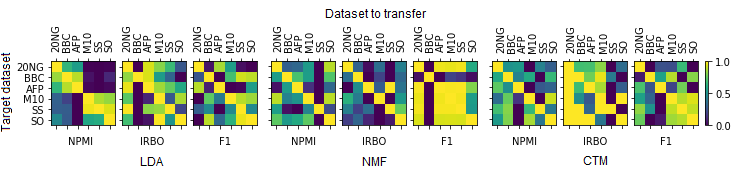
Figure 3: Heatmap matrix representing the performance when transferring the 5 best configurations from a dataset to a target dataset. The average of the runs is computed and each row is normalized between 0 and 1.

The Cost of the Hyperparameter Optimization.

Although optimizing the hyperparameters of a topic model guarantees a fair comparison with other models, this approach is computationally expensive, possibly making it difficult to replicate the results Bianchi and Hovy (2021). In our work, we used BO because it is more efficient than other methods Snoek et al. (2012); Bergstra and Bengio (2012). Yet, the process requires a fair amount of iterations to guarantee the convergence to an optimal solution, especially when the hyperparameter space is large. Moreover, following Terragni et al. (2021), we run the models with the same hyperparameter configuration for 30 times to guarantee robust results. It follows that replicating these results require time and computational resources. In the Appendix, we report an estimation of the cost the hyperparameter optimization.

In light of these observations, we argue that the knowledge that we have acquired for this extensive experimental campaign needs to be exploited and transferred. This will lead to results which are more accurate and obtained more efficiently. As previously mentioned, one direction is to use the best hyperparameter configurations on a dataset to initialize the hyperparameter optimization on the unseen target dataset Feurer et al. (2014). In this paper, we do not discuss this direction in detail, but we will later show that hyperparameter transfer is effective in some cases and it is therefore a promising solution to minimize the computational cost to achieve optimal results on new datasets.

6.2 Hyperparameter Transfer (RS #2)

Hyperparameter consistency across datasets.

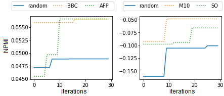
Figure 4: 20NG dataset.

Figure 5: LDA performance in terms on NPMI with MOBO initialized with random configurations or with the configurations transferred from another dataset.

In the following, we report the results related to the hyperparameter transfer to an unseen dataset. This allows us to identify if the best hyperparameters are consistent across all the datasets. Figure 3 shows the results for LDA, CTM and NMF for each metric. Each matrix represents the performance of a model when the best 5 hyperparameter configurations are transferred from a dataset (columns) to the target dataset (rows). We compute the average of the 5 runs and we normalize each row. The diagonal of the matrix is then usually 1, since it represents the best configurations identified by the multi-objective optimization. We report the disaggregated results in the Appendix.

Let us consider the transfer on LDA (first three matrices on the left). Regarding NPMI, when we transfer the configurations from/to 20NG, AFP, and BBC, the topic model obtains results that are similar to the ones discovered by the previous MOBO experiments. Similar observations hold for the datasets M10, SS and SO. We can therefore deduce that the document length has an impact on the discovery of the best hyperparameter configuration for topic coherence. We observe a similar behavior for the IRBO performance, with the exception of the BBC dataset. Although the values of the topic diversity are very close to each other, the long-text datasets usually get similar performance when the hyperparameters are transferred from long-text datasets, and the same holds for short-text datasets.

On the other hand, concerning the F1 performance, we observe a different trend: the configurations coming from BBC, M10, SS and SO seem to be transferable to that group of datasets, while a configuration coming from 20NG or AFP does not guarantee high performance on the previous datasets. This suggests that the document length is not the only feature that needs to be taken into consideration when we transfer the hyperparameters.

Concerning the models NMF and CTM, we can observe different patterns for each metric. For example, if we consider the topic coherence in CTM, the configurations related to datasets 20NG, AFP, BBC and SS have close performances, but distant from M10 and SO. On the other hand, in NMF, the datasets 20NG, M10 and SO appear to be similar to each other, and distant from the others. This might be related to the fact that the topic models are regulated by different types of hyperparameters, which have a different impact on the models’ objectives.

In the considered experiments, we transfer the hyperparameters of a French dataset, i.e. AFP, to English datasets (and vice versa). The AFP’s configurations transferred to another dataset can yield good results, potentially suggesting the existence of language pairs for which the parameter transfer can be near-optimal, given the similiraty of other dataset features. This result is extremely relevant because it would allow us to transfer the known best hyperparameter configurations in low-resource settings, when the best hyperparameter configuration for a dataset in a given language is not available or is expensive to compute.

Random Initial Configurations vs Transferred Initial Configurations.

In this section, we will empirically show what is the effect of using a good set of initial configurations (obtained from the transfer of knowledge from previous experiments), compared to the random initialization.

Figure 5 shows the NPMI performance of LDA for the first 30 MOBO iterations on 20NG (left) and SS (right), when the random initialization is performed (random) or when the MOBO is initialized with the best configurations deriving from another dataset. We transfer the configurations from BBC and AFP for 20NG and the configurations from M10 and SO for SS, since these are the configurations that transferred better for 20NG and SS. Since the first 5 iterations are not ordered chronologically, we report the maximum of them.

We can observe from both figures that, when using the transferred hyperparameters, the MOBO can achieve better results in just a few iterations, outperforming the 30 iterations of the MOBO initialized with random configurations. Therefore using the transferred configurations as initial ones can be helpful to obtain good results in less iterations.

7 Conclusion and Future Work

In this paper, we investigated the role of a multi-objective optimization approach in topic models. We discovered that when we boost the models’ performance at the best of their capabilities, it is not possible to identify an always-winning topic model for each considered objective, thus raising a question on the fairness of the past evaluations and comparisons between topic models. This result is further enforced when additional objectives are jointly considered. Thus, a user that aims to optimize multiple objectives at the same time has to compromise between the different objectives.

We also showed that, in some cases, it is possible to effectively transfer the hyperparameters from a dataset to another. This result paves the way to exciting future research directions. In fact, the hyperparameter transfer allows researchers to avoid several and expensive iterations of hyperparameter optimization. In our experiments, we focused on the transfer of the best hyperparameters for a single metric. However, since we showed that some objectives are competing, a user may require to transfer a hyperparameter configuration that is a combination of more than one objective.

It is worth further investigating which dataset features contribute to a configuration transferable from a dataset to another. Our results suggest that the document length plays a role in the transfer, but other features such as the word and class distributions could be important too. We also showed that the dataset features are likely to be independent of the dataset language, leading to the use of hyperparameter transfer even to unseen datasets in different and low-resource languages.

Ethical Statement

In this research work, we used datasets from the recent literature, and we do not use or infer any sensitive information. The risk of possible abuse of the models and proposed approach is low.

Appendix A Preprocessing details

Datasets SS and SO are already preprocessed. The dataset source refers to Phan et al. (2008) for the dataset details; however the preprocessing pipeline is not available. According to Terragni et al. (2021), datasets 20NG, M10 and BBC have been preprocessed following these steps: tokenization, punctuation and number removal, lemmatization, stop-words removal (using the English stop-words list provided by MALLET), rare words removal and removal of short documents. In particular, they removed the words that have a word frequency less than 50% for 20NG and BBC and less than 0.05% for M10. And they removed the documents with less than 5 words for 20NG and BBC, and less than 3 words for M10. For APF, we followed the same preprocessing pipeline, except we removed the words that have document frequency lower than 1% and higher than 70% and we removed the documents with less than 5 words.

Appendix B The Cost of Hyperparameter Optimization

In Table 3 we report an average estimation of the time expressed in minutes for an iteration of the hyperparameter optimization for the considered models on the 20NG and M10. The overall running time of the optimization can vary depending on the number of documents, the dimensionality of the vocabulary, on the selected hyperparameters (e.g. the number of topics), and of course on the total iterations of the MOBO.

	Datasets
	20NG	M10
LDA	37.51	16.45
NMF	42.16	21.66
CTM	65.98	39.24

Table 3: Estimated minutes to complete one iteration of the MOBO for 20NG and M10 for each model.

Appendix C Hyperparameter Transfer

Figures 6, 7 and 8 show reports the obtained value of the considered metric for the 5 best hyperparameter configurations that we transferred from a dataset (x-axis) to the target dataset ($\rightarrow$ dataset name).

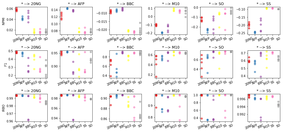
Figure 6: Training for LDA: * $\rightarrow d$ denotes that we transfer hyperparameters from the dataset * to train LDA on the dataset $d$. The x-axis reports the different datasets from which a configuration is transferred.

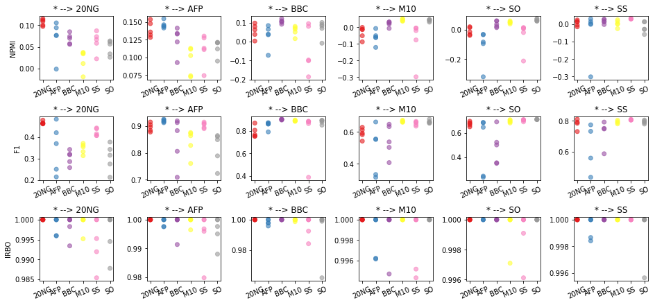
Figure 7: Training for CTM: * $\rightarrow d$ denotes that we transfer hyperparameters from the dataset * to train CTM on the dataset $d$. The x-axis reports the different datasets from which a configuration is transferred.

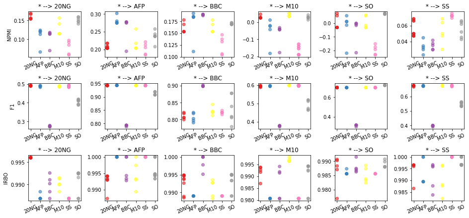
Figure 8: Training for NMF: * $\rightarrow d$ denotes that we transfer hyperparameters from the dataset * to train NMF on the dataset $d$. The x-axis reports the different datasets from which a configuration is transferred.

Appendix D Best hyperparameters configurations

Tables 4, 5 and 6 report the 5 best hyperparameter configurations for LDA for F1, NPMI, and IRBO respectively. Analogous details are provided in Tables 7, 8 and 9, 10, 11 and 12 for CTM and NMF respectively.

Dataset	$\alpha$ prior	$\beta$ prior	# Topics	IRBO	NPMI	F1
20NG	0.0001	10.0000	20	0.95	0.061	0.397
20NG	0.0008	6.3062	26	0.953	0.058	0.424
20NG	0.0121	0.0001	21	0.95	0.057	0.408
20NG	0.0023	1.2349	27	0.961	0.057	0.428
20NG	0.0002	0.0002	19	0.946	0.055	0.403
BBC	0.1007	10.0000	32	0.827	-0.007	0.73
BBC	0.0863	6.7863	48	0.85	-0.007	0.742
BBC	0.1892	1.0099	66	0.861	-0.008	0.746
BBC	0.0080	3.0815	38	0.836	-0.008	0.751
BBC	0.0002	0.0001	46	0.849	-0.009	0.627
AFP	0.0015	0.0001	46	0.976	0.145	0.942
AFP	0.0001	0.0001	49	0.976	0.144	0.94
AFP	0.0054	0.0008	44	0.976	0.143	0.941
AFP	0.0004	0.0010	50	0.977	0.143	0.942
AFP	0.1969	0.0002	46	0.977	0.143	0.944
SS	0.0001	4.8535	147	0.992	-0.093	0.603
SS	0.0003	9.1500	149	0.991	-0.094	0.538
SS	0.0119	10.0000	150	0.991	-0.094	0.567
SS	0.0001	10.0000	150	0.991	-0.095	0.518
SS	0.0001	10.0000	150	0.991	-0.096	0.506
M10	0.0030	10.0000	150	0.974	0.101	0.142
M10	0.0013	10.0000	150	0.972	0.098	0.106
M10	0.0024	10.0000	150	0.973	0.098	0.144
M10	0.0011	10.0000	150	0.974	0.097	0.141
M10	0.0014	10.0000	150	0.972	0.097	0.141
SO	0.0007	10.0000	133	0.97	-0.008	0.093
SO	0.0019	10.0000	138	0.955	-0.012	0.094
SO	0.0004	10.0000	138	0.955	-0.024	0.093
SO	0.0004	10.0000	142	0.94	-0.024	0.093
SO	0.0002	10.0000	142	0.941	-0.025	0.093

Table 4: Best 5 hyperparameter configurations for LDA on each dataset for NPMI.

Dataset	$\alpha$ prior	$\beta$ prior	# Topics	IRBO	NPMI	F1
20NG	0.0001	10.0000	20	0.95	0.061	0.397
20NG	0.0008	6.3062	26	0.953	0.058	0.424
20NG	0.0121	0.0001	21	0.95	0.057	0.408
20NG	0.0023	1.2349	27	0.961	0.057	0.428
20NG	0.0002	0.0002	19	0.946	0.055	0.403
BBC	0.1007	10.0000	32	0.827	-0.007	0.73
BBC	0.0863	6.7863	48	0.85	-0.007	0.742
BBC	0.1892	1.0099	66	0.861	-0.008	0.746
BBC	0.0080	3.0815	38	0.836	-0.008	0.751
BBC	0.0002	0.0001	46	0.849	-0.009	0.627
AFP	0.0015	0.0001	46	0.976	0.145	0.942
AFP	0.0001	0.0001	49	0.976	0.144	0.94
AFP	0.0054	0.0008	44	0.976	0.143	0.941
AFP	0.0004	0.0010	50	0.977	0.143	0.942
AFP	0.1969	0.0002	46	0.977	0.143	0.944
SS	0.0001	4.8535	147	0.992	-0.093	0.603
SS	0.0003	9.1500	149	0.991	-0.094	0.538
SS	0.0119	10.0000	150	0.991	-0.094	0.567
SS	0.0001	10.0000	150	0.991	-0.095	0.518
SS	0.0001	10.0000	150	0.991	-0.096	0.506
M10	0.0030	10.0000	150	0.974	0.101	0.142
M10	0.0013	10.0000	150	0.972	0.098	0.106
M10	0.0024	10.0000	150	0.973	0.098	0.144
M10	0.0011	10.0000	150	0.974	0.097	0.141
M10	0.0014	10.0000	150	0.972	0.097	0.141
SO	0.0007	10.0000	133	0.97	-0.008	0.093
SO	0.0019	10.0000	138	0.955	-0.012	0.094
SO	0.0004	10.0000	138	0.955	-0.024	0.093
SO	0.0004	10.0000	142	0.94	-0.024	0.093
SO	0.0002	10.0000	142	0.941	-0.025	0.093

Table 5: Best 5 hyperparameter configurations for LDA on each dataset for F1.

Dataset	$\alpha$ prior	$\beta$ prior	# Topics	IRBO	NPMI	F1
20NG	0.1483	0.0083	150	0.994	-0.010	0.473
20NG	0.0446	0.0001	150	0.993	-0.005	0.455
20NG	0.0947	0.0002	150	0.993	0.005	0.399
20NG	0.0048	0.2006	150	0.993	-0.003	0.434
20NG	0.1961	0.0001	111	0.993	0.010	0.365
BBC	0.0001	0.0001	150	0.906	-0.021	0.357
BBC	0.0447	10.0000	150	0.906	-0.020	0.691
BBC	0.0001	0.0001	150	0.906	-0.021	0.348
BBC	0.0004	10.0000	150	0.906	-0.020	0.697
BBC	0.0003	0.0071	150	0.906	-0.020	0.325
AFP	0.1668	0.0002	150	0.987	0.103	0.953
AFP	0.0452	0.0001	148	0.987	0.107	0.948
AFP	0.0017	0.0001	149	0.986	0.107	0.943
AFP	0.0006	0.0015	150	0.986	0.107	0.943
AFP	0.0001	0.0001	150	0.986	0.107	0.943
SS	0.0990	0.4641	98	0.997	-0.256	0.557
SS	0.1242	0.0014	150	0.997	-0.273	0.577
SS	0.2860	0.0085	69	0.997	-0.265	0.579
SS	0.3039	0.9328	83	0.997	-0.220	0.611
SS	0.0052	0.3995	149	0.996	-0.236	0.553
M10	0.1483	0.0001	150	0.987	-0.236	0.291
M10	0.1496	0.0187	103	0.985	-0.252	0.556
M10	0.0524	0.2615	102	0.985	-0.239	0.429
M10	0.0130	0.0011	105	0.984	-0.209	0.500
M10	0.0249	0.0001	117	0.984	-0.207	0.510
SO	0.1657	0.0001	64	0.996	-0.302	0.585
SO	0.0863	0.5342	81	0.995	-0.297	0.605
SO	0.0808	0.0037	92	0.993	-0.304	0.607
SO	0.0135	0.4842	68	0.993	-0.264	0.503
SO	0.0223	0.5298	62	0.993	-0.262	0.504

Table 6: Best 5 hyperparameter configurations for LDA on each dataset for IRBO.

Dataset	Activation	Dropout	Learn priors	Learning rate	Momentum	# Layers	# Topics	# Neurons	Optimizer	IRBO	NPMI	F1
20NG	rrelu	0.000	0	0.0001	0.114	1	143	1000	rmsprop	0.989	0.024	0.480
20NG	elu	0.113	1	0.0020	0.489	2	53	600	adam	0.994	0.094	0.467
20NG	elu	0.061	1	0.0001	0.387	2	118	100	rmsprop	0.985	0.044	0.464
20NG	leakyrelu	0.326	1	0.1000	0.808	1	63	400	rmsprop	0.995	0.082	0.464
20NG	rrelu	0.022	0	0.1000	0.200	1	64	200	adam	0.996	0.097	0.462
AFP	leakyrelu	0.274	1	0.0626	0.116	4	148	1000	rmsprop	0.989	0.104	0.926
AFP	rrelu	0.322	1	0.0015	0.900	1	150	1000	rmsprop	0.993	0.101	0.923
AFP	rrelu	0.354	0	0.0440	0.900	3	126	600	rmsprop	0.988	0.113	0.919
AFP	rrelu	0.115	1	0.0207	0.018	4	138	300	adam	0.991	0.112	0.917
AFP	softplus	0.000	0	0.1000	0.755	2	61	900	adam	0.995	0.145	0.913
BBC	rrelu	0.312	0	0.0149	0.420	3	139	900	adam	0.988	0.000	0.901
BBC	selu	0.327	0	0.0025	0.720	3	150	600	adam	0.978	0.062	0.901
BBC	selu	0.000	1	0.0055	0.061	1	9	800	rmsprop	1.000	0.066	0.899
BBC	elu	0.606	0	0.0001	0.482	2	78	300	sgd	0.948	0.075	0.899
BBC	rrelu	0.220	1	0.0013	0.900	1	6	900	rmsprop	1.000	0.004	0.894
M10	elu	0.438	0	0.0012	0.012	1	16	1000	sgd	0.985	0.042	0.674
M10	selu	0.645	0	0.0006	0.748	1	15	800	sgd	0.973	0.048	0.670
M10	elu	0.549	0	0.0025	0.012	1	24	300	rmsprop	0.980	0.026	0.665
M10	elu	0.708	1	0.0066	0.363	1	37	300	adam	0.971	0.023	0.664
M10	elu	0.640	1	0.0003	0.304	1	37	100	sgd	0.964	0.051	0.661
SO	elu	0.367	1	0.0005	0.558	3	22	600	adam	0.990	0.042	0.732
SO	selu	0.126	1	0.0004	0.377	1	44	700	adam	0.987	-0.019	0.721
SO	elu	0.577	1	0.1000	0.134	3	26	400	adadelta	0.972	0.034	0.717
SO	sigmoid	0.727	1	0.0009	0.716	1	23	600	adam	0.974	0.050	0.715
SO	elu	0.000	0	0.0001	0.840	2	19	600	rmsprop	0.996	0.043	0.714
SS	elu	0.452	1	0.0027	0.285	2	44	300	adam	0.991	0.011	0.809
SS	selu	0.777	1	0.0005	0.590	1	127	400	adam	0.977	0.023	0.807
SS	leakyrelu	0.034	1	0.0721	0.054	2	26	800	rmsprop	1.000	-0.009	0.806
SS	selu	0.489	1	0.0057	0.084	2	59	800	rmsprop	0.992	-0.024	0.805
SS	rrelu	0.562	1	0.0014	0.794	1	71	300	rmsprop	0.990	-0.012	0.804

Table 7: Best 5 hyperparameter configurations for CTM on each dataset for F1.

Dataset	Activation	Dropout	Learn priors	Learning rate	Momentum	# Layers	# Topics	# Neurons	Optimizer	IRBO	NPMI	F1
20NG	elu	0.000	0	0.1000	0.859	1	27	1000	rmsprop	0.997	0.115	0.461
20NG	elu	0.127	0	0.0016	0.009	1	30	900	rmsprop	0.996	0.112	0.458
20NG	leakyrelu	0.000	1	0.0052	0.650	2	44	600	rmsprop	0.995	0.109	0.456
20NG	elu	0.000	1	0.0712	0.097	3	49	1000	adam	0.995	0.100	0.424
20NG	leakyrelu	0.356	0	0.0028	0.744	1	22	1000	rmsprop	0.995	0.097	0.409
BBC	softplus	0.000	1	0.0018	0.306	1	18	400	adam	0.994	0.120	0.876
BBC	softplus	0.272	0	0.0002	0.066	1	16	200	sgd	0.977	0.109	0.878
BBC	relu	0.003	1	0.0002	0.067	1	37	700	sgd	0.977	0.106	0.797
BBC	elu	0.000	0	0.0001	0.500	3	10	300	sgd	0.984	0.101	0.890
BBC	elu	0.130	0	0.0001	0.453	4	26	200	sgd	0.972	0.091	0.890
AFP	rrelu	0.000	0	0.1000	0.105	4	129	900	adagrad	0.989	0.155	0.887
AFP	rrelu	0.000	0	0.0495	0.089	3	41	100	rmsprop	0.995	0.146	0.898
AFP	softplus	0.000	0	0.1000	0.755	2	61	900	adam	0.995	0.145	0.913
AFP	relu	0.000	0	0.0075	0.701	1	97	1000	rmsprop	0.994	0.144	0.896
AFP	relu	0.000	1	0.0875	0.856	4	58	600	adam	0.995	0.142	0.911
SS	selu	0.802	1	0.0001	0.781	3	38	100	rmsprop	0.952	0.031	0.757
SS	relu	0.296	0	0.0001	0.640	1	42	100	rmsprop	0.981	0.031	0.773
SS	selu	0.360	0	0.0002	0.688	1	42	700	rmsprop	0.990	0.031	0.801
SS	selu	0.359	0	0.0001	0.643	1	34	800	rmsprop	0.991	0.030	0.802
SS	selu	0.824	1	0.0002	0.469	1	105	400	rmsprop	0.969	0.029	0.802
M10	elu	0.640	1	0.0003	0.304	1	37	100	sgd	0.964	0.051	0.661
M10	selu	0.645	0	0.0006	0.748	1	15	800	sgd	0.973	0.048	0.670
M10	elu	0.438	0	0.0012	0.012	1	16	1000	sgd	0.985	0.042	0.674
M10	leakyrelu	0.393	0	0.0005	0.111	2	22	700	sgd	0.972	0.038	0.648
M10	softplus	0.300	1	0.0006	0.694	2	30	800	sgd	0.974	0.036	0.657
SO	sigmoid	0.013	1	0.0016	0.442	1	18	100	sgd	0.991	0.073	0.701
SO	selu	0.000	1	0.0023	0.130	2	18	300	sgd	0.992	0.070	0.712
SO	relu	0.000	1	0.0005	0.870	2	16	1000	sgd	0.993	0.062	0.679
SO	rrelu	0.041	0	0.0050	0.305	2	19	200	sgd	0.990	0.060	0.690
SO	leakyrelu	0.482	1	0.0004	0.154	1	17	800	sgd	0.987	0.058	0.698

Table 8: Best 5 hyperparameter configurations for CTM on each dataset for NPMI.

Dataset	Activation	Dropout	Learn priors	Learning rate	Momentum	# Layers	# Topics	# Neurons	Optimizer	IRBO	NPMI	F1
20NG	rrelu	0.0238	0	0.0078	0.741	3	5	400	rmsprop	1.000	0.021	0.215
20NG	softplus	0.4102	1	0.0580	0.270	2	5	600	rmsprop	1.000	0.013	0.203
20NG	rrelu	0.0000	1	0.0874	0.389	1	5	400	adagrad	1.000	0.004	0.235
20NG	rrelu	0.0402	0	0.1000	0.552	4	5	100	adagrad	1.000	-0.006	0.197
20NG	leakyrelu	0.0000	1	0.0633	0.385	1	5	500	adam	1.000	0.016	0.242
BBC	rrelu	0.0225	1	0.0676	0.864	4	5	900	adam	1.000	-0.039	0.843
BBC	selu	0.0000	1	0.0055	0.061	1	9	800	rmsprop	1.000	0.066	0.899
BBC	rrelu	0.2199	1	0.0013	0.900	1	6	900	rmsprop	1.000	0.004	0.894
BBC	relu	0.0000	0	0.0005	0.038	1	5	700	adadelta	1.000	-0.433	0.342
BBC	rrelu	0.0177	1	0.0792	0.819	1	5	900	adagrad	1.000	-0.032	0.894
AFP	selu	0.6558	1	0.0060	0.540	1	5	600	rmsprop	1.000	0.051	0.657
AFP	leakyrelu	0.0000	1	0.0712	0.439	3	5	800	adagrad	1.000	0.033	0.667
AFP	rrelu	0.0000	1	0.1000	0.763	4	5	200	adagrad	1.000	0.025	0.665
AFP	leakyrelu	0.0000	0	0.0009	0.532	1	5	400	rmsprop	1.000	0.064	0.666
AFP	rrelu	0.0000	1	0.0712	0.807	2	8	500	adagrad	1.000	0.083	0.781
SS	rrelu	0.0000	1	0.0578	0.455	4	17	700	rmsprop	1.000	-0.030	0.794
SS	selu	0.0000	1	0.0013	0.900	5	5	800	adam	1.000	-0.105	0.549
SS	selu	0.0000	1	0.0006	0.729	1	7	200	adam	1.000	0.005	0.694
SS	relu	0.1055	1	0.0088	0.836	4	5	300	adam	1.000	-0.155	0.530
SS	relu	0.8341	0	0.0010	0.900	2	5	1000	adam	1.000	-0.153	0.523
M10	rrelu	0.0000	0	0.0086	0.791	1	5	700	adam	1.000	-0.083	0.496
M10	leakyrelu	0.0329	0	0.0059	0.214	2	5	700	rmsprop	1.000	-0.101	0.478
M10	selu	0.0000	1	0.0196	0.088	1	5	300	adam	1.000	-0.116	0.490
M10	relu	0.0000	1	0.0489	0.157	1	5	400	adam	1.000	-0.134	0.492
M10	elu	0.6812	1	0.1000	0.013	1	6	300	adam	1.000	-0.073	0.520
SO	softplus	0.3098	1	0.0001	0.527	3	5	600	rmsprop	1.000	-0.135	0.304
SO	rrelu	0.4490	1	0.0167	0.602	1	5	300	rmsprop	1.000	-0.162	0.305
SO	selu	0.5117	0	0.0233	0.752	1	5	400	rmsprop	1.000	-0.147	0.310
SO	elu	0.1316	1	0.0006	0.405	2	5	900	sgd	1.000	-0.052	0.290
SO	softplus	0.2041	1	0.0002	0.312	3	5	1000	rmsprop	1.000	-0.116	0.308

Table 9: Best 5 hyperparameter configurations for CTM on each dataset for IRBO.

Dataset	Reg. factor	L1/L2	Initialization	Regularization	# Topics	IRBO	NPMI	F1
20NG	0.000	1.000	random	H matrix	150	0.993	0.060	0.494
20NG	0.109	0.110	random	H matrix	150	0.992	0.059	0.492
20NG	0.000	1.000	nndsvda	H matrix	150	0.992	0.061	0.491
20NG	0.500	0.000	nndsvda	V matrix	150	0.992	0.061	0.489
20NG	0.001	0.537	random	H matrix	140	0.992	0.064	0.489
BBC	0.336	0.000	nndsvdar	both	5	0.989	0.153	0.901
BBC	0.068	0.156	nndsvd	V matrix	5	0.989	0.153	0.899
BBC	0.000	0.738	nndsvda	both	5	0.989	0.153	0.899
BBC	0.000	0.000	nndsvda	both	5	0.989	0.153	0.899
BBC	0.487	0.000	random	V matrix	5	0.989	0.153	0.899
AFP	0.131	0.000	random	both	150	0.994	0.188	0.944
AFP	0.139	0.280	random	H matrix	147	0.994	0.186	0.944
AFP	0.050	0.991	random	H matrix	150	0.994	0.184	0.943
AFP	0.314	0.000	nndsvdar	H matrix	150	0.995	0.186	0.943
AFP	0.445	0.066	nndsvdar	H matrix	148	0.995	0.185	0.943
SS	0.500	0.507	nndsvda	V matrix	150	0.997	0.022	0.676
SS	0.000	0.174	nndsvd	both	146	0.997	0.019	0.674
SS	0.000	0.021	nndsvdar	H matrix	150	0.997	0.017	0.674
SS	0.015	0.000	nndsvdar	both	150	0.997	0.018	0.674
SS	0.219	0.000	nndsvda	V matrix	150	0.997	0.018	0.673
M10	0.275	0.000	nndsvda	H matrix	150	0.994	-0.191	0.599
M10	0.000	0.408	nndsvdar	both	150	0.994	-0.192	0.598
M10	0.477	0.000	nndsvdar	V matrix	150	0.994	-0.191	0.596
M10	0.025	0.534	nndsvd	V matrix	150	0.994	-0.192	0.596
M10	0.000	0.696	nndsvdar	V matrix	146	0.994	-0.189	0.596
SO	0.390	0.570	nndsvda	V matrix	21	0.977	0.034	0.722
SO	0.428	0.563	nndsvdar	H matrix	46	0.986	-0.075	0.721
SO	0.130	0.739	nndsvd	H matrix	43	0.986	-0.067	0.721
SO	0.140	0.087	random	V matrix	44	0.986	-0.070	0.721
SO	0.395	0.730	nndsvdar	V matrix	25	0.981	-0.004	0.720

Table 10: Best 5 hyperparameter configurations for NMF on each dataset for F1.

Dataset	Reg. factor	L1/L2	Initialization	Regularization	# Topics	IRBO	NPMI	F1
20NG	0.500	0.510	nndsvdar	both	5	0.983	0.169	0.150
20NG	0.423	0.555	nndsvdar	both	5	0.984	0.166	0.156
20NG	0.409	0.303	nndsvda	V matrix	9	0.988	0.156	0.325
20NG	0.312	0.350	nndsvda	both	5	0.980	0.154	0.208
20NG	0.026	0.395	nndsvda	H matrix	10	0.987	0.154	0.339
BBC	0.500	0.788	nndsvda	H matrix	28	0.992	0.190	0.833
BBC	0.429	0.344	nndsvd	both	125	0.959	0.190	0.487
BBC	0.234	0.264	nndsvd	V matrix	26	0.992	0.189	0.818
BBC	0.486	0.000	nndsvd	H matrix	26	0.992	0.189	0.830
BBC	0.465	0.433	nndsvda	H matrix	27	0.992	0.188	0.821
AFP	0.415	0.788	nndsvdar	both	133	0.993	0.302	0.806
AFP	0.426	0.804	nndsvdar	H matrix	20	0.994	0.280	0.900
AFP	0.114	0.078	random	V matrix	24	0.994	0.276	0.906
AFP	0.000	0.705	nndsvdar	both	28	0.994	0.275	0.904
AFP	0.000	0.000	random	V matrix	24	0.994	0.274	0.907
SS	0.379	0.283	nndsvd	both	146	0.994	0.076	0.512
SS	0.179	0.708	nndsvdar	both	99	0.993	0.073	0.543
SS	0.293	0.255	nndsvdar	both	87	0.995	0.073	0.570
SS	0.205	0.477	nndsvd	both	150	0.994	0.072	0.548
SS	0.248	0.319	nndsvdar	both	75	0.995	0.070	0.563
M10	0.000	0.025	random	V matrix	5	0.962	0.051	0.362
M10	0.037	1.000	nndsvdar	V matrix	9	0.994	0.049	0.430
M10	0.120	0.854	nndsvd	H matrix	15	0.989	0.039	0.468
M10	0.031	0.605	nndsvd	V matrix	5	0.981	0.032	0.368
M10	0.080	1.000	nndsvdar	H matrix	5	0.981	0.032	0.369
SO	0.443	0.741	nndsvdar	V matrix	12	0.974	0.071	0.578
SO	0.090	0.673	nndsvdar	both	10	0.975	0.070	0.484
SO	0.182	0.720	nndsvd	V matrix	14	0.975	0.068	0.604
SO	0.440	0.612	nndsvdar	H matrix	13	0.974	0.066	0.587
SO	0.018	0.378	nndsvdar	V matrix	15	0.973	0.064	0.628

Table 11: Best 5 hyperparameter configurations for NMF on each dataset for NPMI.

Dataset	Reg. factor	L1/L2	Initialization	Regularization	# Topics	IRBO	NPMI	F1
20NG	0.250	1.000	random	V matrix	11	0.996	-0.207	0.056
20NG	0.443	0.980	random	V matrix	87	0.996	-0.195	0.056
20NG	0.479	0.607	random	V matrix	124	0.996	-0.193	0.056
20NG	0.204	0.795	random	V matrix	131	0.996	-0.195	0.056
20NG	0.500	0.919	random	V matrix	67	0.996	-0.196	0.056
BBC	0.390	0.786	nndsvd	both	68	1.000	0.077	0.301
BBC	0.281	0.998	random	V matrix	5	1.000	-0.431	0.227
BBC	0.500	1.000	random	both	5	1.000	-0.431	0.227
BBC	0.500	0.478	random	V matrix	57	0.998	-0.416	0.227
BBC	0.142	0.447	random	H matrix	150	0.995	0.101	0.803
AFP	0.335	0.000	random	H matrix	5	1.000	0.203	0.793
AFP	0.372	1.000	nndsvd	V matrix	5	1.000	0.203	0.788
AFP	0.366	0.883	nndsvda	V matrix	5	1.000	0.203	0.788
AFP	0.282	1.000	random	H matrix	5	1.000	0.197	0.791
AFP	0.011	0.000	random	H matrix	5	1.000	0.203	0.793
SS	0.072	0.018	nndsvda	V matrix	5	1.000	0.050	0.400
SS	0.000	0.742	nndsvdar	V matrix	5	1.000	0.050	0.401
SS	0.000	0.849	nndsvda	H matrix	5	1.000	0.050	0.395
SS	0.199	1.000	nndsvdar	V matrix	5	1.000	0.047	0.396
SS	0.323	1.000	nndsvd	V matrix	5	1.000	0.047	0.392
M10	0.500	0.182	random	V matrix	5	0.998	-0.643	0.135
M10	0.215	0.804	random	V matrix	6	0.997	-0.633	0.135
M10	0.430	0.736	random	V matrix	7	0.996	-0.624	0.135
M10	0.092	0.264	random	V matrix	86	0.996	-0.514	0.135
M10	0.140	0.789	random	V matrix	70	0.996	-0.516	0.135
SO	0.278	0.116	nndsvdar	V matrix	150	0.992	-0.231	0.696
SO	0.442	0.000	nndsvd	H matrix	150	0.992	-0.231	0.699
SO	0.500	0.000	random	V matrix	150	0.992	-0.233	0.697
SO	0.429	1.000	nndsvda	H matrix	5	0.991	-0.013	0.312
SO	0.183	0.000	nndsvda	both	150	0.991	-0.227	0.698

Table 12: Best 5 hyperparameter configurations for NMF on each dataset for IRBO.

Appendix E Computing Infrastructure

We ran the experiments on a machine equipped with 4 T1390 GPU, CUDA v11.1, 512GB RAM, Intel(R) Xeon(R) CPU E5-2683 v4 @ 2.10GHz.

References

- Archetti and Candelieri (2019) Francesco Archetti and Antonio Candelieri. 2019. Bayesian Optimization and Data Science. Springer International Publishing.
- Asuncion et al. (2009) Arthur U. Asuncion, Max Welling, Padhraic Smyth, and Yee Whye Teh. 2009. On Smoothing and Inference for Topic Models. In Proceedings of the Twenty-Fifth Conference on Uncertainty in Artificial Intelligence (UAI), pages 27–34, Montreal, QC, Canada.
- Bergstra and Bengio (2012) James Bergstra and Yoshua Bengio. 2012. Random Search for Hyper-Parameter Optimization. Journal of Machine Learning Research, 13:281–305.
- Bianchi and Hovy (2021) Federico Bianchi and Dirk Hovy. 2021. On the gap between adoption and understanding in nlp. In Findings of the Association for Computational Linguistics: ACL-IJCNLP 2021, pages 3895–3901.
- Bianchi et al. (2021a) Federico Bianchi, Silvia Terragni, and Dirk Hovy. 2021a. Pre-training is a hot topic: Contextualized document embeddings improve topic coherence. In Proceedings of the 59th Annual Meeting of the Association for Computational Linguistics and the 11th International Joint Conference on Natural Language Processing, ACL/IJCNLP 2021, pages 759–766. Association for Computational Linguistics.
- Bianchi et al. (2021b) Federico Bianchi, Silvia Terragni, Dirk Hovy, Debora Nozza, and Elisabetta Fersini. 2021b. Cross-lingual Contextualized Topic Models with Zero-shot Learning. In Proceedings of the 16th Conference of the European Chapter of the Association for Computational Linguistics, pages 1676–1683. Association for Computational Linguistics.
- Blei (2012) David M Blei. 2012. Probabilistic topic models. Communications of the ACM, 55(4):77–84.
- Blei et al. (2003) David M. Blei, Andrew Y. Ng, and Michael I. Jordan. 2003. Latent Dirichlet Allocation. Journal of Machine Learning Research, 3:993–1022.
- Boyd-Graber et al. (2017) Jordan L. Boyd-Graber, Yuening Hu, and David M. Mimno. 2017. Applications of Topic Models. Foundations and Trends in Information Retrieval, 11(2-3):143–296.
- Burkhardt and Kramer (2019) Sophie Burkhardt and Stefan Kramer. 2019. Decoupling Sparsity and Smoothness in the Dirichlet Variational Autoencoder Topic Model. Journal of Machine Learning Research, 20(131):1–27.
- Chang et al. (2009) Jonathan Chang, Jordan L. Boyd-Graber, Sean Gerrish, Chong Wang, and David M. Blei. 2009. Reading Tea Leaves: How Humans Interpret Topic Models. In Advances in Neural Information Processing Systems 22: 23rd Annual Conference on Neural Information Processing Systems (NIPS), pages 288–296, Vancouver, BC, Canada. Curran Associates, Inc.
- Devlin et al. (2019) Jacob Devlin, Ming-Wei Chang, Kenton Lee, and Kristina Toutanova. 2019. BERT: pre-training of deep bidirectional transformers for language understanding. In Proceedings of the 2019 Conference of the North American Chapter of the Association for Computational Linguistics: Human Language Technologies, NAACL-HLT 2019, pages 4171–4186. Association for Computational Linguistics.
- Dieng et al. (2020) Adji Bousso Dieng, Francisco J. R. Ruiz, and David M. Blei. 2020. Topic modeling in embedding spaces. Trans. Assoc. Comput. Linguistics, 8:439–453.
- Ding et al. (2018) Ran Ding, Ramesh Nallapati, and Bing Xiang. 2018. Coherence-Aware Neural Topic Modeling. In Proceedings of the 2018 Conference on Empirical Methods in Natural Language Processing, pages 830–836, Brussels, Belgium. Association for Computational Linguistics.
- Doan and Hoang (2021) Thanh-Nam Doan and Tuan-Anh Hoang. 2021. Benchmarking neural topic models: An empirical study. In Findings of the Association for Computational Linguistics: ACL-IJCNLP 2021, pages 4363–4368, Online. Association for Computational Linguistics.
- Feurer et al. (2014) Matthias Feurer, Jost Tobias Springenberg, and Frank Hutter. 2014. Using Meta-Learning to Initialize Bayesian Optimization of Hyperparameters. In Proceedings of the International Workshop on Meta-learning and Algorithm Selection, co-located with 21st European Conference on Artificial Intelligence (MetaSel@ECAI 2014), volume 1201 of CEUR Workshop Proceedings, pages 3–10, Prague, Czech Republic. CEUR-WS.org.
- González-Santos et al. (2021) Carlos González-Santos, Miguel A. Vega-Rodríguez, and Carlos J. Pérez. 2021. Addressing topic modeling with a multi-objective optimization approach based on swarm intelligence. Knowledge-Based Systems, 225:107113.
- Greene and Cunningham (2006) Derek Greene and Pádraig Cunningham. 2006. Practical Solutions to the Problem of Diagonal Dominance in Kernel Document Clustering. In Proceedings of the 23rd International Conference on Machine learning (ICML’06), pages 377–384. ACM Press.
- Griffiths and Steyvers (2004) Thomas L. Griffiths and Mark Steyvers. 2004. Finding scientific topics. Proceedings of the National Academy of Sciences, 101(suppl 1):5228–5235.
- Kandasamy et al. (2020) Kirthevasan Kandasamy, Karun Raju Vysyaraju, Willie Neiswanger, Biswajit Paria, Christopher R. Collins, Jeff Schneider, Barnabás Póczos, and Eric P. Xing. 2020. Tuning Hyperparameters without Grad Students: Scalable and Robust Bayesian Optimisation with Dragonfly. Journal of Machine Learning Research, 21:81:1–81:27.
- Khalifa et al. (2013) Osama Khalifa, David Wolfe Corne, Mike Chantler, and Fraser Halley. 2013. Multi-objective Topic Modeling. In Evolutionary Multi-Criterion Optimization, pages 51–65, Berlin, Heidelberg. Springer Berlin Heidelberg.
- Korencic et al. (2018) Damir Korencic, Strahil Ristov, and Jan Snajder. 2018. Document-based topic coherence measures for news media text. Expert Systems with Applications, 114:357–373.
- Lau et al. (2014) Jey Han Lau, David Newman, and Timothy Baldwin. 2014. Machine reading tea leaves: Automatically evaluating topic coherence and topic model quality. In Proceedings of the 14th Conference of the European Chapter of the Association for Computational Linguistics, EACL 2014, pages 530–539.
- Lim and Buntine (2014) Kar Wai Lim and Wray L. Buntine. 2014. Bibliographic Analysis with the Citation Network Topic Model. In Proceedings of the Sixth Asian Conference on Machine Learning, ACML 2014.
- Mockus et al. (1978) Jonas Mockus, Vytautas Tiesis, and Antanas Zilinskas. 1978. The application of bayesian methods for seeking the extremum. Towards global optimization, 2(117-129):2.
- Nan et al. (2019) Feng Nan, Ran Ding, Ramesh Nallapati, and Bing Xiang. 2019. Topic modeling with wasserstein autoencoders. In Proceedings of the 57th Conference of the Association for Computational Linguistics, ACL 2019, Florence, Italy, July 28- August 2, 2019, Volume 1: Long Papers, pages 6345–6381. Association for Computational Linguistics.