Large Charges on the Wilson Loop in $\mathcal{N}=4$ SYM:
II. Quantum Fluctuations, OPE, and Spectral Curve

Abstract

We continue our study of large charge limits of the defect CFT defined by the half-BPS Wilson loop in planar $\mathcal{N}=4$ supersymmetric Yang-Mills theory. In this paper, we compute $1/J$ corrections to the correlation function of two heavy insertions of charge $J$ and two light insertions, in the double scaling limit where the charge $J$ and the ’t Hooft coupling $\lambda$ are sent to infinity with the ratio $J/\sqrt{\lambda}$ fixed. Holographically, they correspond to quantum fluctuations around a classical string solution with large angular momentum, and can be computed by evaluating Green’s functions on the worldsheet. We derive a representation of the Green’s functions in terms of a sum over residues in the complexified Fourier space, and show that it gives rise to the conformal block expansion in the heavy-light channel. This allows us to extract the scaling dimensions and structure constants for an infinite tower of non-protected dCFT operators. We also find a close connection between our results and the semi-classical integrability of the string sigma model. The series of poles of the Green’s functions in Fourier space corresponds to points on the spectral curve where the so-called quasi-momentum satisfies a quantization condition, and both the scaling dimensions and the structure constants in the heavy-light channel take simple forms when written in terms of the spectral curve. These observations suggest extensions of the results by Gromov, Schafer-Nameki and Vieira on the semiclassical energy of closed strings, and in particular hint at the possibility of determining the structure constants directly from the spectral curve.

1 Introduction

Wilson loops are fundamental observables in any gauge theory. They provide a natural basis of gauge-invariant operators, play the role of order parameter for the confinement-deconfinement transition, and satisfy a set of non-perturbative Schwinger-Dyson equations called the loop equations [1, 2], which are especially useful in two dimensions [4, 5].

In the maximally supersymmetric gauge theory in four dimensions known as $\mathcal{N}=4$ supersymmetric Yang-Mills (SYM) theory, one can define generalizations of the usual Wilson loop that couple to scalar fields and preserve a fraction of supersymmetry. Of particular importance among them is the half-BPS Wilson loop, which couples to a single scalar field and is defined on a circular (or infinite straight line) contour. Thanks to extensive research in the past few years, it has become clear that the half-BPS Wilson loop provides an ideal testing ground for various non-perturbative approaches in quantum field theory.

Firstly, the half-BPS Wilson loop preserves a one-dimensional superconformal group $OSp(4^{\ast}|4)$ [6, 7, 8] and provides a canonical example of a one-dimensional defect conformal field theory (CFT) [9]. This enables one to study the correlation functions of insertions on the Wilson loop using both analytical and numerical bootstrap techniques [10, 11, 12, 13]. Secondly, there exists a “topological” subsector of this defect CFT (dCFT) in which the correlation functions become position-independent and can be computed analytically as nontrivial functions of the ’t Hooft coupling $\lambda(\equiv g_{\rm YM}^{2}N)$ using the method of supersymmetric localization [14, 15, 16, 17, 18]. This led to a rigorous determination of an infinite set of defect conformal data on the half-BPS Wilson loop, which provided important inputs for the conformal bootstrap analysis. Thirdly, the half-BPS Wilson loop in the fundamental representation is holographically dual to an open string minimal surface extending in the AdS₂ subspace of AdS${}_{5}\times S^{5}$. Using this dual representation, one can study the correlation functions of insertions at strong coupling via perturbation theory of the string sigma model [19]. Finally, the operator insertions on the half-BPS Wilson loop can be mapped to states in an integrable open spin chain and their spectrum can in principle be determined exactly using integrability techniques [8, 20, 21, 22, 23]. The three- and higher-point functions also seem amenable to the integrability machinery [24, 25], in particular to the so-called hexagon formalism [26, 27, 28], although more work is needed to fully develop the formalism.

The study of the half-BPS Wilson loop also allows one to explore the cross-fertilization of different techniques. For instance, the correlation functions in the topological subsector computed from supersymmetric localization in [14, 15] can be recast into an integral of Q-functions, which are the most basic quantities in the integrability formalism [29]. This strongly hints at the applicability of integrability to correlation functions and also suggests a deep connection between integrability and supersymmetric localization. In addition, a recent study [13] demonstrated that one can determine conformal data to remarkable numerical precision by combining the numerical conformal bootstrap and the spectral data computed from integrability. Alternatively, one can use the conformal bootstrap to extend the results from perturbation theory: this has been demonstrated explicitly in [11], which computed the three-loop corrections at strong coupling by imposing the crossing symmetry of the four-point functions. A similar analysis at weak coupling has not been fully developed but a few direct perturbative results, which would provide starting points of such computations, are available in the literature [30, 31, 25, 32, 33]. Furthermore, the half-BPS Wilson loop provides a simple example of defect renormalization group flow, which connects the ordinary Wilson loop without scalar couplings to the half-BPS loop [34]. The defect renormalization group flow can be studied both at weak and strong couplings [35, 36] (see also [37, 38, 39] for related recent works) and it allows one to explicitly check the monotonicity of the defect entropy, which was proven recently in [40].

The goal of this paper and its companion [41] is to explore a connection to yet another non-perturbative approach—the large charge expansion of conformal field theory. Starting from the seminal works [42, 43], general properties of the large charge sector in interacting CFTs with global symmetries have been actively explored in recent years using effective field theory techniques and treating the inverse of the charge as a small expansion parameter [44, 45, 46, 47, 48]. In the Wilson loop defect CFT, the simplest analog of the large charge sector is given by the correlation functions of two insertions with R-charge $J$ and several light insertions in the limit

$$J\to\infty\,,\qquad\lambda\to\infty\,,\qquad\frac{J}{\sqrt{\lambda}}:\text{ fixed}\,.$$ (1.1)

In this regime, the role of the large charge effective field theory is played by a probe string action in AdS${}_{5}\times S^{5}$, which becomes classical in the large $J$ limit. As we demonstrated in the previous paper [41], the leading large charge answer for the correlation functions can be computed by evaluating light vertex operators on a nontrivial classical string solution with large angular momentum, which was constructed in [8, 49, 50]. In special kinematics, we can compare the results from holography with exact results from supersymmetric localization [14] and verify the agreement of the two approaches.

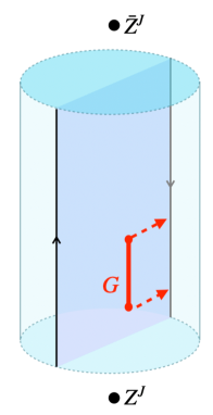
Figure 1: A sketch of the setup. In the radial quantization, a single BPS Wilson loop is mapped to two straight lines in $R\times S^{3}$ (which are connected with each other at future and past infinities) while the operator insertions with large charges ($Z^{J}$ and $\bar{Z}^{J}$ in the figure) are mapped to a state defined on $S^{3}$ in the presence of the Wilson lines. This setup is holographically dual to a string worldsheet anchored at the Wilson lines at the boundary (the blue strip in the figure). To compute the four-point function, we evaluate the Green’s function (the red segment in the figure) and push the endpoints to the boundary. This gives the correlation function of two heavy insertions and two light fluctuations on the worldsheet. The picture shows the case where the endpoints are sent to the same boundary on the strip, which gives the four-point function in the “heavy-heavy-light-light” ordering. One may also send the endpoints to opposite boundaries, which gives the “heavy-light-heavy-light” ordering of the correlation function. See Figure 4 for more details.

In this paper, we consider the leading $1/J$ corrections to the results computed in the previous paper. In the double scaling limit (1.1), this is equivalent to studying $1/\sqrt{\lambda}$ corrections, which correspond to quantum fluctuations on the string worldsheet. For simplicity, we focus on the four-point functions— namely, the correlation functions of two large charge insertions and two light insertions. We compute them by evaluating the Green’s functions of light fluctuations around the classical string solution with large angular momentum, and sending the endpoints of the Green’s functions to the boundaries of the worldsheet (see Figure 1). The results for the Green’s functions are given by integrals over Fourier modes, which take the following schematic form,

$$G(r,\tau;r^{\prime},\tau^{\prime})\overset{r>r^{\prime}}{\sim}\int_{-\infty}^{\infty}dk\,e^{ik(\tau-\tau^{\prime})}\frac{g^{R}(r;k)g^{L}(r^{\prime};k)}{\left<g^{R},g^{L}\right>}\,.$$ (1.2)

Here, $G$ is the Green’s function, $r$ and $\tau$ are the coordinates on the worldsheet, $g^{L}$ and $g^{R}$ are solutions to the same second-order differential equation (which turns out to be of the Lamé type) that satisfy $g^{L}\to 0$ $(g^{R}\to 0)$ at the left (right) boundary of the worldsheet, and, finally, $\left<g^{R},g^{L}\right>$ is the Wronskian of the two solutions (which is a position-independent function of $k$). The integrand has poles in the upper-half $k$ plane where the Wronskian vanishes. Picking up the residues from those poles, we can rewrite (1.2) as a discrete sum, which turns out to precisely reproduce the conformal block expansion in the heavy-light channel. This allows us to read off conformal data of the Wilson loop defect CFT, including the conformal dimensions of (infinitely many) non-protected heavy operators and the “heavy-heavy-light” structure constants.

In addition, the discrete sum representation has a tantalizing connection to integrability, and in particular to the spectral curve and the so-called quasi-momentum. The spectral curve is one of the fundamental concepts in the classical integrability of the string sigma model: it encodes infinitely many conserved charges as its period integrals and it arises as the semiclassical limit of the Bethe equations, in which the Bethe roots—i.e., the solutions to the Bethe equations—clump up and form branch cuts [51, 52]. The quasi-momentum $p(x)$ is a function on the spectral curve that satisfies certain analyticity properties and the integral of $p(x)d(x+1/x)$ gives the period integrals on the spectral curve.

As we will show below, each term in the discrete sum corresponds to a point on the spectral curve satisfying a “quantization condition” $p(x_{n})=n\pi$ with $n\in\mathbb{N}$, and the defect CFT data in the heavy-light channel is given by simple functions on the spectral curve. A similar observation was made by Gromov, Schafer-Nameki and Vieira [53], who developed an efficient method to compute the semiclassical energy of closed strings by expressing it as a function on the spectral curve. A novelty of our results is that we find that the structure constants, not just the energy of the string (or, equivalently, the conformal dimension), simplify when written in terms of the spectral parameter $x$. This hints at an extension of the analysis of [53] to the three-point functions and suggests it may be possible to compute them directly from the spectral curve and classical integrability, without explicit reference to string solutions.

Outline of the paper.

The rest of the paper is organized as follows: In Section 2, we summarize the basics of the four-point functions of insertions on the half-BPS Wilson loop, including the superconformal Ward identities and the definition of the large charge limit. We also present the main results for the four point functions that we will derive in later sections. In Section 3, we review the classical string solution describing the large charge insertions and compute quadratic fluctuations around it. We also explain how to extract the four-point function of two large charge insertions and two light insertions from Green’s functions of light fluctuations. In Section 4, we derive an integral representation of Green’s functions and later recast it into a discrete sum by picking up the residues of the poles in the complexified Fourier space. The discrete sum can be identified with the conformal block expansion in the heavy-light channel. Using this fact, in Section 5 we read off the conformal dimensions of infinitely many heavy operators and the “heavy-heavy-light” structure constants. We also study the behavior of the correlators and OPE data at small and large $J/\sqrt{\lambda}$. In Section 6, we discuss a connection to integrability. We show that each term in the sum corresponds to a point on the spectral curve satisfying a quantization condition and derive simple expressions for the conformal dimensions and the structure constants as functions of the spectral parameter. In Section 7, we conclude and discuss future directions. Several appendices are included to explain technical details.

2 Four-point defect correlators with large charge

2.1 Preliminaries

This paper continues the analysis started in [41]. Let us briefly review the setup. We start with the (Maldacena-)Wilson operator in $\mathcal{N}=4$ SYM:

$$\mathcal{W} \equiv\frac{1}{N}\text{Tr P}\text{ exp}\left(\oint\left(iA_{\mu}(x)\dot{x}^{\mu}+|\dot{x}|Y^{I}\Phi_{I}(x)\right)dt\right).$$ (2.1)

Here $x^{\mu}(t)$ is a closed contour in $\mathbb{R}^{4}$ (we work in Euclidean signature), $Y^{I}(t)$ is a closed contour in $S^{5}$ (i.e., $\delta_{IJ}Y^{I}Y^{J}=1$, where $I,J=1,\ldots,6$), and the trace is taken in the fundamental representation of the gauge group, which we take to be $U(N)$. The gauge field $A_{\mu}$ and the scalars $\Phi_{I}$ transform in the adjoint representation of $U(N)$. We are interested in the special case of the half-BPS Wilson line, for which the spacetime contour is an infinite straight line and $Y^{I}$ is a point in $S^{5}$ (equivalently, one may consider a circular contour after a conformal transformation). For concreteness, we let $x^{\mu}(t)=(t,0,0,0)$ and $Y^{I}\Phi_{I}=\Phi_{6}$. The symmetries preserved by the Wilson line form the one-dimensional superconformal group, $OSp(4^{*}|4)\subset PSU(2,2|4)$, which includes $16$ supercharges and the bosonic subgroup $SL(2,\mathbb{R})\times SO(3)\times SO(5)$. Here, $SL(2,\mathbb{R})$ are the conformal symmetries of the Wilson line, $SO(3)$ are the spacetime rotations about the line, and $SO(5)$ is the R-symmetry subgroup that rotates the scalars not coupled to the Wilson line.

The Wilson line defines a one-dimensional defect CFT, in which correlation functions of defect local operators are obtained by inserting local adjoint operators along the spacetime contour [8, 31, 30, 19, 35, 14, 25, 15, 10, 36, 16, 23, 11, 13, 33]. Explicitly, the correlation function of $n$ defect operators $O_{i}(t_{i})\equiv O_{i}(x(t_{i}))$ inserted in order on the line (i.e., $t_{m}<t_{m^{\prime}}$ if $m<m^{\prime}$) is defined by

$$\braket{O_{1}(t_{1})\ldots O_{n}(t_{n})} \equiv\Big{\langle}\frac{1}{N}\text{Tr }\left[W_{n+1,n}O_{n}(t_{n})W_{n,n-1}\ldots W_{21}O_{1}(t_{1})W_{10}\right]\Big{\rangle}_{\mathcal{N}=4\text{ SYM}},$$ (2.2)

$$W_{ji} \equiv\text{P}e^{\int_{t_{i}}^{t_{j}}(A_{0}+\Phi_{6})dt},$$ (2.3)

where $t_{0}\equiv-\infty$, $t_{n+1}\equiv\infty$. These correlators have the normalization $\braket{1}=\braket{\mathcal{W}}_{\mathcal{N}=4{\text{ SYM}}}=1$. One may also consider correlation functions involving insertions of local gauge invariant operators away from the Wilson line, but in this paper we focus on correlators involving only defect insertions.

The Wilson line defect correlators satisfy the axioms of a 1d CFT (see Appendix A of [54]). For instance, the two- and three-point functions of primary operators $O_{1}$, $O_{2}$ and $O_{3}$ take the form:

$$\braket{O_{1}(t_{1})O_{2}(t_{2})} =\frac{\mathcal{N}_{O_{1}O_{2}}}{t_{21}^{2\Delta_{1}}}\delta_{\Delta_{1}\Delta_{2}},$$ (2.4)

$$\braket{O_{1}(t_{1})O_{2}(t_{2})O_{3}(t_{3})} =\frac{\mathcal{C}_{O_{1}O_{2}O_{3}}}{t_{21}^{\Delta_{1}+\Delta_{2}-\Delta_{3}}t_{32}^{\Delta_{2}+\Delta_{3}-\Delta_{1}}t_{31}^{\Delta_{3}+\Delta_{1}-\Delta_{2}}}, t_{1}<t_{2}<t_{3}.$$ (2.5)

Here, $t_{ij}\equiv t_{i}-t_{j}$ is the signed Euclidean distance on the line and $\mathcal{N}_{O_{1}O_{2}}$ and $\mathcal{C}_{O_{1}O_{2}O_{3}}$ are the two-point and three-point (i.e., OPE) coefficients. The normalized OPE coefficients are given by $\mathcal{C}_{O_{1}O_{2}O_{3}}/(\mathcal{N}_{O_{1}O_{1}^{\dagger}}\mathcal{N}_{O_{2}O_{2}^{\dagger}}\mathcal{N}_{O_{3}O_{3}^{\dagger}})^{\frac{1}{2}}$.

In 1d CFTs, because operators on a line cannot be moved continuously around each other without becoming coincident, three-point and higher-point functions generically depend on the circle-ordering of the operators. Thus, the OPE coefficient in (2.5) is defined with a particular order. By circular permutation, it satisfies $\mathcal{C}_{O_{1}O_{2}O_{3}}=\mathcal{C}_{O_{2}O_{3}O_{1}}=\mathcal{C}_{O_{3}O_{1}O_{2}}$ and likewise $\mathcal{N}_{O_{1}O_{2}}=\mathcal{N}_{O_{2}O_{1}}$. Given that the Wilson line defect CFT is parity invariant and unitary, there are also relations between configurations of correlators with different circle-orderings. For instance, assuming the primaries are parity eigenstates, the OPE coefficients with different orderings will differ at most by a minus sign: $\mathcal{C}_{O_{1}O_{2}O_{3}}=(-1)^{P_{1}+P_{2}+P_{3}}\mathcal{C}_{O_{3}O_{2}O_{1}}$, where $(-1)^{P_{i}}$ is the parity of $O_{i}$. Furthermore, the time-reversal property of the adjoint map, $\braket{O_{n}^{\dagger}(t_{n})\ldots O_{1}^{\dagger}(t_{1})}=\braket{O_{1}(-t_{1})\ldots O_{n}(-t_{n})}^{*}$, implies $\mathcal{C}_{O_{1}O_{2}O_{3}}^{*}=\mathcal{C}_{O_{3}^{\dagger}O_{2}^{\dagger}O_{1}^{\dagger}}$. The relations between different configurations of higher-point functions will in general be more complicated.

There are two classes of “elementary operators” on the Wilson line dCFT that we will work with. The first class consists of the chiral primaries of the form $(\epsilon\cdot\Phi)^{L}$ where $\Phi=(\Phi_{1},\ldots,\Phi_{5})$ are the scalars that do not couple to the Wilson line, $L$ is a non-negative integer, and $\epsilon\in\mathbb{C}^{5}$ is a polarization vector satisfying $\epsilon^{2}=0$. This operator transforms in the rank $L$ symmetric traceless representation of $SO(5)$ and its dimension is protected and equal to its R-charge, $\Delta=L$. For the rank-$1$ symmetric traceless (i.e., the fundamental) representation, we can also denote the operators by $\Phi_{a}$, $a=1,\ldots,5$. For concreteness, we will often phrase our discussion in terms of the specific chiral primaries

$$Z \equiv\Phi_{4}+i\Phi_{5}, \bar{Z} \equiv\Phi_{4}-i\Phi_{5}.$$ (2.6)

The second class of operators we will work with are the displacement operators, $\mathbb{D}_{a}$, $a=1,2,3$. Displacement operators exist in any dCFT due to the breaking of translational symmetry [9]. They generate local orthogonal translations of the defect. On the Wilson line, the displacement operators take the explicit form $\mathbb{D}_{a}\equiv iF_{0a}+D_{a}\Phi_{6}$, where $F_{0a}$ is the gauge field strength and $D_{a}$ is the covariant derivative. They transform in the fundamental representation of $SO(3)$ and have protected dimension $\Delta=2$. We can also use the alternative notation $\mu\cdot\mathbb{D}$, where $\mu\in\mathbb{C}^{3}$ is a polarization vector satisfying $\mu^{2}=0$.

Previous results in the large charge sector of the Wilson line dCFT.

In [41], we studied correlators of chiral primaries in the dCFT in which two of the primaries have “large” R-charge. More precisely, we chose the R-charges of the two distinguished primaries to be $J$ and took the following sequence of double-scaling limits,

$$\begin{aligned} &1)&&N\to\infty\text{ with $g$ and $J$ held fixed}\\ &2)&&J,g\to\infty\text{ with $\mathcal{J}$ held fixed}\end{aligned}\hskip 56.9055pt\text{(large charge limit),}$$ (2.7)

where $g$ and $\mathcal{J}$ are defined by

$$g\equiv\frac{\sqrt{\lambda}}{4\pi}\,,\qquad\qquad\mathcal{J}\equiv\frac{J}{g}\,.$$ (2.8)

We call operators whose R-charges scale in proportion with the coupling $g$ in the large charge limit “heavy” and operators whose quantum numbers do not scale with $g$ “light.”

In [41], we studied the leading large charge behavior of the two-point function $\braket{Z^{J}\bar{Z}^{J}}$ and higher-point functions $\braket{Z^{J}\bar{Z}^{J}\prod_{i}Z^{\ell_{i}}\prod_{j}\bar{Z}^{\bar{\ell}_{j}}}$ using AdS/CFT. The two-point function was found to be

$$\braket{Z^{J}(t_{L})\bar{Z}^{J}(\bar{t}_{L})} =\frac{\mathcal{N}_{Z^{J}\bar{Z}^{J}}}{(t_{L}-\bar{t}_{L})^{2J}}, \mathcal{N}_{Z^{J}\bar{Z}^{J}}=(2gc)^{2J}e^{8g(\mathbb{E}(c^{2})-\mathbb{E}(0))},$$ (2.9)

where the parameter $c^{2}$ is related to $\mathcal{J}$ by:

$$\frac{\mathcal{J}}{4} =\mathbb{K}(c^{2})-\mathbb{E}(c^{2}),$$ (2.10)

and $\mathbb{K}(c^{2})$ and $\mathbb{E}(c^{2})$ are the complete elliptic integrals of the first and second kind. Meanwhile, the higher-point functions take the simplest form consistent with conformal symmetry:

$$\frac{\braket{Z^{J}(t_{L})\bar{Z}^{J}(\bar{t}_{L})\prod_{i=1}^{m}Z^{\ell_{i}}(t_{i})\prod_{j=1}^{n}\bar{Z}^{\bar{\ell}_{j}}(\bar{t}_{j})}}{\braket{Z^{J}(t_{L})\bar{Z}^{J}(\bar{t}_{L})}} =\frac{(t_{L}-\bar{t}_{L})^{2\ell_{\rm tot}}(2gc)^{2\ell_{\rm tot}}}{\prod_{i=1}^{m}(t_{i}-\bar{t}_{L})^{2\ell_{i}}\prod_{j=1}^{n}(\bar{t}_{i}-t_{L})^{2\bar{\ell}_{i}}}\delta_{\ell_{\rm tot}\bar{\ell}_{\rm tot}},$$ (2.11)

where $\ell_{\rm tot}\equiv\sum_{i=1}^{m}\ell_{i}$ and $\bar{\ell}_{\rm tot}\equiv\sum_{j=1}^{n}\bar{\ell}_{j}$.

We also studied the large charge limit of the two-point function $\braket{\tilde{\Phi}^{J}\tilde{\Phi}^{J}}$ and higher-point functions $\braket{\tilde{\Phi}^{J}\tilde{\Phi}^{J}\prod_{i}\tilde{\Phi}^{\ell_{i}}}$, where $\tilde{\Phi}^{\ell}\equiv(\epsilon(t)\cdot\Phi(t))^{\ell}$ is a “topological” chiral primary whose polarization vector $\epsilon(t)$ is correlated with its position in such a way that its correlation functions are independent of position. These observables are related to the ones in (2.9) and (2.11) because, at leading order in large charge, the topological primary truncates to a sum of powers of $Z$ and $\bar{Z}$ only— namely, $\tilde{\Phi}^{\ell}\sim(\epsilon_{Z}(t)Z(t)+\epsilon_{\bar{Z}}(t)\bar{Z}(t))^{\ell}$ for an appropriate choice of $\epsilon_{Z},\epsilon_{\bar{Z}}$. Correlators of the topological operators can be studied using localization[14, 15] and, accordingly, in [41] we expressed the topological correlators in terms of an “emergent” $J\times J$ matrix model that we could analyze in the large charge limit using the usual saddle point techniques. The result for $\braket{\tilde{\Phi}^{J}\tilde{\Phi}^{J}}$ agreed with (2.9), and the topological higher-point functions reproduced the appropriate linear combinations of the correlators in (2.11).

Finally, also using localization, we were able to relate certain topological correlators to the generalized Bremsstrahlung function, $B_{J}$, whose leading and subleading behavior in the large charge limit was determined in [50, 56]. As a special case, this allowed us to determine the following large charge OPE coefficient to subleading order:

$$\frac{\mathcal{C}_{Z^{\ell}Z^{J}\bar{Z}^{J+\ell}}^{2}}{\mathcal{N}_{Z^{\ell}\bar{Z}^{\ell}}\mathcal{N}_{Z^{J}\bar{Z}^{J}}\mathcal{N}_{Z^{J+\ell}\bar{Z}^{J+\ell}}}=\frac{(g\pi c^{2})^{\ell}}{\ell!}\left(1+\frac{\ell(\ell+1)}{4g}\left[\frac{3}{4\pi}+\frac{1-c^{2}}{c^{2}\mathbb{E}(c^{2})}\right]+O(1/g^{2})\right).$$ (2.12)

These OPE coefficients satisfy $\mathcal{C}_{ZZ^{J}\bar{Z}^{J+\ell}}=\mathcal{C}_{Z^{J}Z\bar{Z}^{J+\ell}}=\mathcal{C}_{\bar{Z}\bar{Z}^{J}Z^{J+\ell}}$ and are real, as required by parity, R-symmetry and time-reversal.

Four-point correlators in the large charge sector.

In this work, we continue to study defect correlators in which two chiral primaries have large R-charge, now extending the analysis to subleading order in the large charge expansion. We will use AdS/CFT to compute the following four-point functions:

$$\frac{\braket{\epsilon_{1}\cdot\Phi(t_{1})\text{ }\epsilon_{2}\cdot\Phi(t_{2})(\epsilon_{3}\cdot\Phi(t_{3}))^{J}(\epsilon_{4}\cdot\Phi(t_{4}))^{J}}}{\braket{(\epsilon_{3}\cdot\Phi(t_{3}))^{J}(\epsilon_{4}\cdot\Phi(t_{4}))^{J}}}=\frac{2g}{\pi}\frac{\epsilon_{1}\cdot\epsilon_{2}}{t_{12}^{2}}\left[G_{1}(\chi)+\zeta G_{2}(\chi)+\xi G_{3}(\chi)\right],$$ (2.13)

$$\frac{\braket{\mu_{1}\cdot\mathbb{D}(t_{1})\text{ }\mu_{2}\cdot\mathbb{D}(t_{2})(\epsilon_{3}\cdot\Phi(t_{3}))^{J}(\epsilon_{4}\cdot\Phi(t_{4}))^{J}}}{\braket{(\epsilon_{3}\cdot\Phi(t_{3}))^{J}(\epsilon_{4}\cdot\Phi(t_{4}))^{J}}}=\frac{12g}{\pi}\frac{\mu_{1}\cdot\mu_{2}}{t_{12}^{4}}G_{4}(\chi).$$ (2.14)

Here, $\chi$ is the conformally invariant cross-ratio given by

$$\chi \equiv\frac{t_{12}t_{34}}{t_{13}t_{24}}, \frac{1}{1-\chi} =\frac{t_{13}t_{24}}{t_{14}t_{23}}, \frac{1-\chi}{\chi} =\frac{t_{14}t_{23}}{t_{12}t_{34}},$$ (2.15)

and $\xi$ and $\zeta$ are the $SO(5)$ invariant cross-ratios of the polarization vectors given by

$$\xi \equiv\frac{\epsilon_{1}\cdot\epsilon_{3}\text{ }\epsilon_{2}\cdot\epsilon_{4}}{\epsilon_{1}\cdot\epsilon_{2}\text{ }\epsilon_{3}\cdot\epsilon_{4}}, \zeta \equiv\frac{\epsilon_{1}\cdot\epsilon_{4}\text{ }\epsilon_{2}\cdot\epsilon_{3}}{\epsilon_{1}\cdot\epsilon_{2}\text{ }\epsilon_{3}\cdot\epsilon_{4}}.$$ (2.16)

The dependence of the conformally invariant functions, $G_{i}(\chi)$, on $N$, $g$ and $J$ is left implicit in our notation. In the large charge expansion (after taking the planar limit), each $G_{i}(\chi)$ is written as a series in $1/g$ with a general functional dependence on $\mathcal{J}$ at each order. Note that, since $\mathcal{J}=J/g$, this large charge scaling limit effectively resums an infinite number of terms in the ordinary perturbation theory in powers of $1/g$ with $J$ finite.

The general form of (2.13) and (2.14) is fixed by the $SL(2,\mathbb{R})$, $SO(5)$ and $SO(3)$ symmetries. The normalizations are chosen based on the observation that when either $J\to 0$ or $\chi\to 0$, then the normalized four-point functions reproduce the two-point functions of the unit chiral and displacement operators. In particular, $\chi\to 0$ corresponds to the OPE limit $t_{1}\to t_{2}$ or $t_{3}\to t_{4}$, which is dominated by the exchange of the identity operator between the two light and the two heavy operators. The two-point functions are known [57]:

$$\braket{\epsilon_{1}\cdot\Phi(t_{1})\epsilon_{2}\cdot\Phi(t_{2})}=n_{1}(g)\frac{\epsilon_{1}\cdot\epsilon_{2}}{t_{12}^{2}}, \braket{\mu_{1}\cdot\mathbb{D}(t_{1})\mu_{2}\cdot\mathbb{D}(t_{2})}=6n_{1}(g)\frac{\mu_{1}\cdot\mu_{2}}{t_{12}^{4}}.$$ (2.17)

The relative normalization of these correlators is fixed by supersymmetry (because $\Phi_{i}$ and $\mathbb{D}_{a}$ are in the same supermultiplet of $OSp(4^{*}|4)$) and the coefficient, $n_{1}(g)$, is known exactly from localization [57, 14]. In the planar limit, one finds $n_{1}(g)=\frac{2g}{\pi}\frac{I_{2}(4\pi g)}{I_{1}(4\pi g)}$. For our purposes, we will only need the first two terms in the planar strong coupling limit ($N\to\infty$, $g\gg 1$):

$$n_{1}(g) =\frac{2g}{\pi}\left(1-\frac{3}{8\pi g}+\ldots\right).$$ (2.18)

Matching (2.17) with (2.13)-(2.14), it follows that $G_{1},G_{4}\to 1-\frac{3}{8\pi g}+O(1/g^{2})$ and $G_{2},G_{3}\to 0$, as either $\chi\to 0$ (for any $J$), or $J\to 0$.

It will often be convenient to let $Z^{J}$ and $\bar{Z}^{J}$ serve as the charge $J$ operators in (2.13) and (2.14), where $Z$ and $\bar{Z}$ were defined in (2.6). Thus, instead of the general correlators in (2.13)-(2.14), we will typically work with the four correlators

$$\frac{\braket{\Phi_{i}(t_{1})\Phi_{j}(t_{2})Z^{J}(t_{3})\bar{Z}^{J}(t_{4})}}{\braket{Z^{J}(t_{3})\bar{Z}^{J}(t_{4})}} =\frac{2g}{\pi}\frac{1}{t_{12}^{2}}G_{1}(\chi)\delta_{ij},$$ (2.19)

$$\frac{\braket{Z(t_{1})\bar{Z}(t_{2})Z^{J}(t_{3})\bar{Z}^{J}(t_{4})}}{\braket{Z^{J}(t_{3})\bar{Z}^{J}(t_{4})}} =\frac{4g}{\pi}\frac{1}{t_{12}^{2}}G_{Z\bar{Z}}(\chi),$$ (2.20)

$$\frac{\braket{\bar{Z}(t_{1})Z(t_{2})Z^{J}(t_{3})\bar{Z}^{J}(t_{4})}}{\braket{Z^{J}(t_{3})\bar{Z}^{J}(t_{4})}} =\frac{4g}{\pi}\frac{1}{t_{12}^{2}}G_{\bar{Z}Z}(\chi),$$ (2.21)

$$\frac{\braket{\mathbb{D}_{a}(t_{1})\mathbb{D}_{b}(t_{2})Z^{J}(t_{3})\bar{Z}^{J}(t_{4})}}{\braket{Z^{J}(t_{3})\bar{Z}^{J}(t_{4})}} =\frac{12g}{\pi}\frac{1}{t_{12}^{4}}G_{4}(\chi)\delta_{ab},$$ (2.22)

where we define

$$G_{Z\bar{Z}}(\chi) \equiv G_{1}(\chi)+G_{2}(\chi), G_{\bar{Z}Z}(\chi)\equiv G_{1}(\chi)+G_{3}(\chi).$$ (2.23)

The leading order behavior of (2.20)-(2.21) is included in (2.11). In the present work, we will determine the first subleading correction of (2.20)-(2.21) and the leading behavior of (2.19) and (2.22).

We make a few additional comments about (2.19)-(2.22): The scalars $\Phi_{i}$, $i=1,2,3$, which are orthogonal to $Z$, $\bar{Z}$ and $\Phi_{6}$, possess a residual $SO(3)\subset SO(6)$ R-symmetry. Furthermore, the four operators of interest are all parity even and under the adjoint map satisfy $\Phi_{i}^{\dagger}=\Phi_{i}$, $\mathbb{D}_{a}^{\dagger}=\mathbb{D}_{a}$ and $(Z^{L})^{\dagger}=\bar{Z}^{L}$. Finally, it should be emphasized that there are three inequivalent configurations the four operators on the line can be in, $\chi\in(-\infty,0)$, $\chi\in(0,1)$, and $\chi\in(1,\infty)$, as illustrated in Figure 2. Via analytic continuation from these configurations, each four-point function defines three generically distinct multi-valued complex functions with singularities at $\chi=0,1,\infty$ .

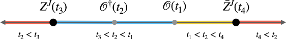
a. Operators on the line…

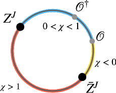
b. … and circle

Figure 2: The four operators on the Wilson line can be in one of three distinct configurations. a. Using the conformal transformations and parity, we can put $Z^{J}(t_{3})$, $\bar{Z}^{J}(t_{4})$ and the first light operator $\mathcal{O}(t_{1})$ at any three points on the line satisfying $t_{3}<t_{1}<t_{4}$. The three configurations of the four-point function are then distinguished by the location of the second light operator: $t_{3}<t_{2}<t_{1}$, $t_{1}<t_{2}<t_{4}$, and $t_{2}<t_{3}$ or $t_{4}<t_{2}$. In terms of the cross-ratio, these correspond to $0<\chi<1$, $\chi<0$, and $\chi>1$. b. The different configurations can also be visualized by compactifying the line to a circle.

Superconformal Ward identities.

Before we commence the analysis of the defect correlators, we note that they are not independent. Specifically, the functions $G_{i}(\chi)$ are related by crossing symmetry and supersymmetry. Firstly, interchanging $1\leftrightarrow 2$ in (2.15) sends $\chi\leftrightarrow\chi/(\chi-1)$ and it therefore follows from (2.19)-(2.22) that

$$G_{1}(\chi) =G_{1}\left(\frac{\chi}{\chi-1}\right), G_{\bar{Z}Z}(\chi) =G_{Z\bar{Z}}\left(\frac{\chi}{\chi-1}\right), G_{4}(\chi) =G_{4}\left(\frac{\chi}{\chi-1}\right).$$ (2.24)

Thus, one can study the $G_{i}(\chi)$ on the restricted interval $\chi\in(0,2)$ and extend them to $\chi\in\mathbb{R}$ using (2.24), or study $G_{i}(\chi)$ on $\chi\in\mathbb{R}$ and use (2.24) as a consistency check.

Less trivially, the correlator in (2.13) satisfies superconformal Ward identities, which may succinctly be written [10]:

$$0 =\left(\frac{\partial\mathcal{A}}{\partial\zeta_{1}}+\frac{1}{2}\frac{\partial\mathcal{A}}{\partial\chi}\right)\biggr{\rvert}_{\zeta_{1}=\chi}=\left(\frac{\partial\mathcal{A}}{\partial\zeta_{2}}+\frac{1}{2}\frac{\partial\mathcal{A}}{\partial\chi}\right)\biggr{\rvert}_{\zeta_{2}=\chi}.$$ (2.25)

Here, $\mathcal{A}\equiv G_{1}(\chi)+\frac{1}{\zeta_{1}\zeta_{2}}G_{3}(\chi)+\frac{(1-\zeta_{1})(1-\zeta_{2})}{\zeta_{1}\zeta_{2}}G_{2}(\chi)$ is the conformally invariant part of the RHS of (2.13) and $\zeta_{1}$ and $\zeta_{2}$ are an alternative parametrization of the $SO(5)$ invariants related to $\xi$ and $\zeta$ by $\xi\equiv\frac{1}{\zeta_{1}\zeta_{2}}$ and $\zeta\equiv\frac{(1-\zeta_{1})(1-\zeta_{2})}{\zeta_{1}\zeta_{2}}$. Evaluating (2.25) explicitly, we get the following two ODEs,

$$\left(\chi\frac{d}{d\chi}-2\right)G_{3}(\chi)=\left(\chi(\chi-1)\frac{d}{d\chi}+2\right)G_{2}(\chi)=-\chi^{2}\frac{dG_{1}}{d\chi}.$$ (2.26)

These equations allow us to solve for $G_{2}(\chi)$ and $G_{3}(\chi)$, and therefore for $G_{Z\bar{Z}}$ and $G_{\bar{Z}Z}$, in terms of $G_{1}(\chi)$, after using input from the OPE limit and the localization result (2.12) to fix the initial conditions. The details of this calculation are given in Section 4.2.2.

Since the unit scalar $\Phi_{i}$ and displacement operator $\mathbb{D}_{a}$ are in the same superconformal multiplet, the correlators in (2.13) and (2.14) are also related by Ward identities [10]. In principle, one can also determine $G_{4}$ in terms of $G_{1}$, just like $G_{Z\bar{Z}}$ and $G_{\bar{Z}Z}$. We will instead study the scalar and displacement correlators independently. This will serve as a test of the consistency of our analysis via the dual string.

2.2 Summary of explicit results for the four-point functions

We close this preliminary section by collecting our final results for the four-point functions. They are accessible without a detailed understanding of the derivations in Sections 3 and 4.

The conformally invariant functions $G_{i}(\chi)$ are naturally expressed as series over the “fluctuation energies” $E_{n}$. These are determined by the quantization condition

$$\int_{1}^{E_{n}}dE\rho(E)=|n|,$$ (2.27)

where the “energy density”, $\rho(E)$, is

$$\rho(E)\equiv\frac{2}{\pi}\frac{\mathbb{K}(c^{2})E^{2}-\mathbb{E}(c^{2})}{\sqrt{E^{2}-1}\sqrt{E^{2}+c^{2}-1}}.$$ (2.28)

Note that the integral in (2.27) converges at $E=1$ for both the edge case $c=0$, for which $\rho(E)=1$, and the general case $c\in(0,1)$, for which $\rho(E)\sim 1/\sqrt{E-1}$ as $E\to 1^{+}$. It is also convenient to define the “form factor”, $f(E)$:

$$f(E)\equiv\frac{\pi}{4}\frac{E(E^{2}+c^{2}-1)}{\mathbb{K}(c^{2})E^{2}-\mathbb{E}(c^{2})}.$$ (2.29)

From the semiclassical analysis of the fluctuations of the dual string in Sections 3-4, we will find that $G_{1}(\chi)$ and $G_{4}(\chi)$ are given by

$$G_{1}(\chi) =\frac{\chi^{2}}{|1-\chi|}\sum_{n\in\mathbb{Z}}\text{sgn}(1-\chi)^{n}f(E_{n})e^{-E_{n}|\log|1-\chi||},$$ (2.30)

$$G_{4}(\chi) =\frac{\chi^{4}}{(1-\chi)^{2}}\sum_{n\in\mathbb{Z}}\text{sgn}(1-\chi)^{n+1}f(E_{n})\frac{E_{n}^{2}-1}{6}e^{-E_{n}|\log|1-\chi||}.$$ (2.31)

Furthermore, $G_{Z\bar{Z}}(\chi)$ and $G_{\bar{Z}Z}(\chi)$ are obtained from $G_{1}(\chi)$ and the Ward identities; the explicit results are given in (4.54)-(4.57).

As discussed in detail in Section 5, these series representations are directly related to the conformal block expansion in the heavy-light channel, and the energies $E_{n}$ and form factors $f(E_{n})$ encode the anomalous dimensions and OPE coefficients of the exchanged operators. The expressions (2.30)-(2.31) are valid for all $\chi\in\mathbb{R}$, except at $\chi=2$, where the $G_{i}(\chi)$ are smooth but their series representations do not converge (as explained in Section 4.2.1, this is related to the radius of convergence of the OPE). It is interesting to note that consistency with the limiting behavior $G_{1}(\chi),G_{4}(\chi)\to 1$ as $\chi\to 0$, as required by the fact that in this limit the OPE of the two light or two heavy operators is dominated by the exchange of the identity, implies that we should have

$$\sum_{n\in\mathbb{Z}}f(E_{n})e^{-E_{n}|\log(1-\chi)|}\stackrel{{\scriptstyle\chi\rightarrow 0}}{{\sim}}\frac{1}{\chi^{2}}\,,$$ (2.32)

$$\sum_{n\in\mathbb{Z}}f(E_{n})\frac{E_{n}^{2}-1}{6}e^{-E_{n}|\log(1-\chi)|}\stackrel{{\scriptstyle\chi\rightarrow 0}}{{\sim}}\frac{1}{\chi^{4}}\,.$$

We will explicitly check towards the end of Section 4.2.1 that these indeed hold, based on the large $n$ behavior of the energies $E_{n}$ and form factors $f(E_{n})$. This is a non-trivial test of the crossing symmetry of our results.

The four-point functions and the OPE data can also be studied analytically at both small $\mathcal{J}$ ($c^{2}\to 0^{+}$) and large $\mathcal{J}$ ($c^{2}\to 1^{-}$), as discussed in Section 5.2. The expansion of the four-point functions in small $c^{2}$ involves polylogarithms. Meanwhile, in the $c^{2}\to 1$ (${\cal J}\to\infty$) limit, the behavior of the four-point functions depends significantly on whether they are in the “heavy-heavy-light-light” ($\chi<1$) or the “heavy-light-heavy-light” ($\chi>1$) configurations: the correlators in the latter configuration vanish while the correlators in the former configuration attain finite limits given by Bessel functions. See Figures 12, 13 and 14 for plots of $G_{1}(\chi)$, $G_{Z\bar{Z}}(\chi)$ and $G_{4}(\chi)$ as functions of $\chi$ for representative values of $c^{2}$, including the edge cases $c^{2}=0$ and $c^{2}=1$.

3 Semiclassical analysis of the dual string

We will compute the next-to-leading order terms in the large charge expansion of the four point functions in (2.19)-(2.22) by studying the semiclassical fluctuations of the string that is holographically dual to the Wilson line with $Z^{J}$ and $\bar{Z}^{J}$ inserted. We first sketch the basic idea in Section 3.1, and then fill in the details in Sections 3.2-3.3 and Section 4.

3.1 Preview

Invoking AdS/CFT, we can schematically write the defect four-point function of two heavy operators $Z^{J}$, $\bar{Z}^{J}$ and two light operators, $\mathcal{O}$ ($\equiv Z$, $\bar{Z}$, $\Phi_{i}$, or $\mathbb{D}_{a}$) and $\mathcal{O}^{\dagger}$, as a string path integral:

$$\braket{\mathcal{O}(t_{1})\mathcal{O}^{\dagger}(t_{2})Z^{J}(t_{3})\bar{Z}^{J}(t_{4})}=\frac{\int\mathcal{D}\Psi e^{-S[\Psi]}v^{J}_{Z}(t_{3})v^{J}_{\bar{Z}}(t_{4})v_{\mathcal{O}}(t_{1})v_{\mathcal{O}^{\dagger}}(t_{2})}{\int\mathcal{D}\Psi e^{-S[\Psi]}}.$$ (3.1)

Here, $\int\mathcal{D}\Psi$ denotes integration over the fields of the superstring sigma model (which we denote collectively by $\Psi$) whose bosonic components are the coordinates of the string in AdS${}_{5}\times S^{5}$, $S[\Psi]$ is the string action, and $v_{Z}$, $v_{\bar{Z}}$, $v_{\mathcal{O}}$ and $v_{\mathcal{O}^{\dagger}}$ are vertex operators dual to $Z$, $\bar{Z}$, $\mathcal{O}$ and $\mathcal{O}^{\dagger}$. In accordance with the “extrapolate dictionary”, we define the vertex operator $v_{\mathcal{O}}$ corresponding to the Wilson line defect operator $\mathcal{O}$ by evaluating the dual field $\Psi_{\mathcal{O}}$ at the point on the boundary of the worldsheet where $\mathcal{O}$ is located. Schematically,

$$v_{\mathcal{O}}(t)\equiv\lim_{z\to 0^{+}}\frac{2g}{z^{\Delta}}\Psi_{\mathcal{O}}(t,z),$$ (3.2)

where $z$ is a particular bulk coordinate that together with $t$ parametrizes the string worldsheet (with boundary at $z=0$), and $\Delta$ is the dimension of $\mathcal{O}$ in the dCFT.

Taking the planar limit in (3.1) picks out the disk topology and taking the large $g$ limit means the path integral is dominated by its saddle point. Without the two large charge insertions, the saddle point would be a classical string extending in an AdS₂ subspace of AdS₅ and sitting at a point on $S^{5}$. With the two large charge insertions $Z^{J}$ and $\bar{Z}^{J}$, the saddle point solution is a classical string, $\Psi_{\rm cl}$, that carries angular momentum $J$ along the circle in $S^{5}$ dual to $Z$. This solution extremizes the “total” action, which includes the contribution of the vertex operators:

$$S_{\rm tot}[\Psi]\equiv S[\Psi]-J\log\left(v_{Z}(t_{3})v_{\bar{Z}}(t_{4})\right).$$ (3.3)

The string tension is $2g$, so the two terms are the same order in the large charge limit.

We reviewed the classical string dual to the Wilson loop with $Z^{J}$ and $\bar{Z}^{J}$ in [41], which was discussed previously in [8, 49, 50]. We computed the action and the vertex operators dual to $Z$ and $\bar{Z}$ on the classical solution, which determined the leading large charge behavior of the two-point and higher-point functions in (2.9) and (2.11). In this work, we go beyond the leading order and therefore need to take into account the fluctuations about the classical string. Letting $\Psi=\Psi_{\rm cl}+\delta\Psi$, we expand $S_{\rm tot}$ to quadratic order in the fluctuation modes:

$$S_{\rm tot}[\Psi_{\rm cl}+\delta\Psi] =S_{\rm tot}[\Psi_{\rm cl}]+\underbrace{\frac{1}{2}\frac{\delta^{2}S_{\rm tot}}{\delta\Psi\delta\Psi}\biggr{\rvert}_{\Psi_{\rm cl}}\delta\Psi\delta\Psi}_{\equiv S_{2}[\delta\Psi]}+O(\delta\Psi^{3}).$$ (3.4)

We will see in Section 3.2 that there are four distinct bosonic fluctuation modes, corresponding to the four types of defect operators on the Wilson line appearing in (2.19)-(2.22). We will not study the fermionic modes.

From (3.1), it follows that the four-point function normalized by the large charge two-point function is given by

$$\frac{\braket{\mathcal{O}(t_{1})\mathcal{O}^{\dagger}(t_{2})Z^{J}(t_{3})\bar{Z}^{J}(t_{4})}}{\braket{Z^{J}(t_{3})\bar{Z}^{J}(t_{4})}}=\underbrace{v_{\mathcal{O}}(t_{1})v_{\mathcal{O}^{\dagger}}(t_{2})\big{\rvert}_{\Psi_{\rm cl}}}_{\rm classical}+\underbrace{W_{\mathcal{O}\mathcal{O}^{\dagger}}(t_{1},t_{2})}_{\rm fluctuation}+O(g^{0}),$$ (3.5)

where we define the boundary-to-boundary propagator

$$W_{\mathcal{O}\mathcal{O}^{\dagger}}(t_{1},t_{2}) \equiv(2\Delta-1)^{2}\lim_{\begin{subarray}{c}z_{1}\to 0^{+}\\ z_{2}\to 0^{+}\end{subarray}}\frac{2g}{z_{1}^{\Delta}}\frac{2g}{z_{2}^{\Delta}}G_{\mathcal{O}\mathcal{O}^{\dagger}}(t_{1},z_{1};t_{2},z_{2})$$ (3.6)

in terms of the bulk-to-bulk propagator

$$G_{\mathcal{O}\mathcal{O}^{\dagger}}(t_{1},z_{1};t_{2},z_{2})\equiv\frac{\int\mathcal{D}\delta\Psi\text{exp}\left(-S_{2}[\delta\Psi]\right)\delta\Psi_{\mathcal{O}}(t_{1},z_{1})\delta\Psi_{\mathcal{O}^{\dagger}}(t_{2},z_{2})}{\int\mathcal{D}\delta\Psi\text{exp}\left(-S_{2}[\delta\Psi]\right)}.$$ (3.7)

Because $S_{2}$ is proportional to the string tension, the bulk-to-bulk propagator is proportional to its inverse, and the fluctuation piece in (3.5) is suppressed relative to the classical piece by $1/g$. Thus, to determine the subleading correction to the large charge four-point functions using AdS/CFT, we need to determine the quadratic action of the fluctuations, compute the bulk-to-bulk propagators, and then send the two bulk points to the boundary.

We will compute the boundary-to-boundary propagators by first solving the Green’s equations satisfied by the bulk-to-bulk propagators. This is the most technical step of the analysis and is the focus of Section 4. The classical string is not homogeneous, unlike the AdS₂ string dual to the Wilson line without insertions. Nonetheless, since the classical string is symmetric under translations parallel to the boundary in global coordinates, we can take the Fourier transform with respect to the boundary global coordinate, in which case the Green’s equations reduce to ODEs in the bulk global coordinate. The ODEs turn out to be of the Jacobi form of the Lamé equation, the solutions of which are known and given in terms of the theta functions. This lets us write explicit integral representations of the propagators. Moreover, we may write the boundary-to-boundary propagators as sums over the residues at the poles, which take particularly simple forms when written in terms of the fluctuation energies of the fluctuations. The series representations of the boundary-to-boundary propagators can be interpreted either as sums over stationary waves on the classical string, which lets us make contact with integrability in Section 6, or as sums over primaries in the the conformal block expansions of the four-point defect correlators, which lets us extract dCFT OPE data in Section 5.

One could also study the subleading behavior of the two-point function that we normalize by in (3.5), by evaluating a functional determinant that takes the schematic form

$$\braket{Z^{J}(t_{3})\bar{Z}^{J}(t_{4})} \propto\underbrace{e^{-S_{\rm tot}[\Psi_{\rm cl}]}}_{\rm classical}\underbrace{\left(\text{Det}\frac{\delta^{2}S_{\rm tot}}{\delta\Psi\delta\Psi}\Big{\rvert}_{\Psi_{\rm cl}}\right)^{-\frac{1}{2}}}_{\rm fluctuation}\left(1+O(1/g)\right).$$ (3.8)

The classical contribution was computed in [41] and is given in eq. (2.9). The calculation of the fluctuation determinant is a non-trivial problem whose solution we will not pursue in this work.

The above sketch of the semiclassical analysis suppresses many details, including the standard steps of picking a suitable gauge and coordinates, redefining fields, simplifying the quadratic action, and keeping track of how these choices affect the dictionary given schematically in (3.5)-(3.7). In the remainder of this section, we will derive the quadratic action of the bosonic fluctuation modes in detail, identify the Green’s equations satisfied by the bulk-to-bulk propagators, and formulate the precise dictionary between the defect correlators and the boundary-to-boundary propagators.

3.2 Quadratic action for the fluctuations

We begin by choosing coordinates for AdS${}_{5}\times S^{5}$. We will use Euclidean signature throughout. First, we introduce the embedding coordinates $X^{A}$, $A=1,\ldots,6$ for AdS₅ and $Y^{I}$, $I=1,\ldots,6$ for $S^{5}$. These satisfy $\eta_{AB}X^{A}X^{B}=-1$ and $\delta_{IJ}Y^{I}Y^{J}=1$, where $\eta_{AB}$ is the Minkowski metric tensor on $\mathbb{R}^{5,1}$ (with mostly plus convention), and $\delta_{IJ}$ is the standard Kronecker symbol on $\mathbb{R}^{6}$. The metric on AdS${}_{5}\times S^{5}$ may then be written:

$$ds^{2}=ds_{\text{AdS}_{5}}^{2}+ds_{S^{5}}^{2},$$ (3.9)

$$ds_{\text{AdS}_{5}}^{2}=\eta_{AB}dX^{A}dX^{B}\,,\qquad ds_{S^{5}}^{2}=\delta_{IJ}dY^{I}dY^{J}.$$

Next, we parametrize the embedding coordinates in a way that is adapted to studying the fluctuations of the dual string. It will be convenient to foliate AdS₅ by AdS${}_{2}\times S^{2}$ slices:

$$X^{a} =\frac{x^{a}}{1-\frac{1}{4}x^{2}}, (X^{4},X^{5},X^{6}) =\frac{1+\frac{1}{4}x^{2}}{1-\frac{1}{4}x^{2}}\left(\sinh{\rho},\cosh{\rho}\sinh{\tau},\cosh{\rho}\cosh{\tau}\right).$$ (3.10)

Here $\rho,\tau\in\mathbb{R}$ are the bulk and Euclidean time coordinates on the AdS₂ slices and $x^{a}\in\mathbb{R}$, $a=1,2,3$, are three orthogonal coordinates with norm $x\equiv\sqrt{x^{a}x^{a}}$. If we decompose $x^{a}$ into radial and angular coordinates, then the two angular coordinates are coordinates on the $S^{2}$ slices and the radial coordinate $x$ parametrizes the different $S^{2}\times AdS_{2}$ slices. Similarly, it will be convenient to foliate $S^{5}$ by $S^{3}\times S^{1}$ slices:

$$Y^{i} =\frac{\cos{\bar{\theta}}\bar{y}^{i}}{1+\frac{1}{4}\bar{y}^{2}},\hskip 28.45274ptY^{6}=\frac{\cos{\bar{\theta}}(1-\frac{1}{4}\bar{y}^{2})}{1+\frac{1}{4}\bar{y}^{2}}, Y^{4}+iY^{5} =\sin{\bar{\theta}}e^{i\bar{\phi}}.$$ (3.11)

Here $\bar{\phi}\in[0,2\pi)$ is the azimuthal angle on the $S^{1}$ slices corresponding to rotations in the $Y^{4}-Y^{5}$ plane, $\bar{y}^{i}\in\mathbb{R}$, $i=1,2,3$, are stereographic coordinates on the $S^{3}$ slices with norm $\bar{y}\equiv\sqrt{\bar{y}^{i}\bar{y}^{i}}$, and $\bar{\theta}\in[0,\pi)$ parametrizes the different $S^{3}\times S^{1}$ slices. We have written the coordinates on $S^{5}$ with bars to distinguish them from redefined coordinates that will appear later. In terms of the $x^{a}$, $\rho$, $\tau$ and $\bar{y}^{i}$, $\bar{\theta}$, $\bar{\phi}$ coordinates, the metrics on Euclidean AdS₅ and $S^{5}$ are

$$ds_{\text{AdS}_{5}}^{2} =\frac{\left(1+\frac{1}{4}x^{2}\right)^{2}}{\left(1-\frac{1}{4}x^{2}\right)^{2}}\left(d\rho^{2}+\cosh^{2}{\rho}d\tau^{2}\right)+\frac{dx^{a}dx^{a}}{\left(1-\frac{1}{4}x^{2}\right)^{2}},$$ (3.12)

$$ds_{S^{5}}^{2} =d\bar{\theta}^{2}+\sin^{2}{\bar{\theta}}d\bar{\phi}^{2}+\cos^{2}{\bar{\theta}}\frac{d\bar{y}^{j}d\bar{y}^{j}}{\left(1+\frac{1}{4}\bar{y}^{2}\right)^{2}}.$$ (3.13)

Now we turn to the string in AdS${}_{5}\times S^{5}$ that is dual to the Wilson line with $Z^{J}$ and $\bar{Z}^{J}$ inserted. We take the spacetime contour of the Wilson line to be a pair of antiparallel, antipodal lines located at the boundary of AdS₅ at $\rho\to\pm\infty$ (one may later perform a conformal transformation to the infinite straight line or circular loop). The contour at $x^{a}=0$ and $\rho\to+\infty$ runs in the positive $\tau$ direction, the contour at $x^{a}=0$ and $\rho\to-\infty$ runs in the negative $\tau$ direction, and $Z^{J}$ and $\bar{Z}^{J}$ are located at $\tau=-\infty$ and $\tau=\infty$, respectively. This configuration in global coordinates has manifest translational symmetry along $\tau$. The classical string dual to this operator was discussed in [8, 49, 50] and reviewed in [41]. To summarize, the string forms a strip in AdS₅ that stretches between the two antipodal lines at $\rho\to\pm\infty$ and partly wraps an $S^{2}$ in $S^{5}$, carrying angular momentum $J$. Since the $S^{5}$ embedding coordinates $Y_{I}$ are dual to the scalars $\Phi_{I}$, and since the Wilson line couples to $\Phi_{6}$ and $Z$ and $\bar{Z}$ are chiral combinations of $\Phi_{4}$ and $\Phi_{5}$, the $S^{2}$ wrapped by the string is given by $(Y^{4})^{2}+(Y^{5})^{2}+(Y^{6})^{2}=1$. With $\bar{y}^{i}=0$ in (3.11), $\bar{\theta}$ and $\bar{\phi}$ are its polar and azimuthal angles.

With $\rho$ and $\tau$ serving as the worldsheet coordinates, the classical dual string is given by:

$$x^{a} =0, \bar{y}^{i} =0, \sin\bar{\theta} =\sin\theta_{\rm cl}(\rho)\equiv\frac{c}{\cosh{\rho}}, \bar{\phi} =\phi_{\rm cl}(\tau)\equiv\phi_{0}-i\tau.$$ (3.14)

Here, the parameter $c\in[0,1)$, which we introduced for convenience in (2.9), determines the maximum polar angle of the string as well as the angular momentum of the string in the $Y^{4}-Y^{5}$ plane. Fixing the angular momentum to be $J$ yields the condition (2.10). Finally, the parameter $\phi_{0}$ in (3.14) is a modulus of the classical solution. This modulus played an important role in [41], but a limited one in the present analysis. When mapping the string observables to the dCFT observables, one should integrate over the modulus to ensure that the string observables are dual to CFT observables in an R-charge eigenstate rather than a coherent state. The integration ensures that correlators not having equal numbers of $Z$ and $\bar{Z}$ are zero, and also gives rise to non-trivial combinatorial factors when the chiral primaries are non-zero linear combinations of both $Z$ and $\bar{Z}$. However, in the computation of the correlators in (2.19)-(2.22), the integration over $\phi_{0}$ is trivial and we will ignore it.

We are interested in the bosonic fluctuations about the classical solution in (3.14). We will work with the Nambu-Goto action and choose the static gauge such that $\rho$ and $\tau$ are not dynamical and serve as the worldsheet coordinates. For notational convenience, we package them into $\sigma^{\mu}\equiv(\rho,\tau)$, and let $\partial_{\mu}\equiv\partial/\partial\sigma^{\mu}$. We denote the AdS₂ metric by $h_{\mu\nu}$ and the metric induced on the classical string by $\gamma_{\mu\nu}$, which are explicitly

$$h_{\mu\nu} \equiv\text{diag}\left(1,\cosh^{2}{\rho}\right),$$ (3.15)

$$\gamma_{\mu\nu} \equiv h_{\mu\nu}+\partial_{\mu}\theta_{\rm cl}\partial_{\nu}\theta_{\rm cl}+\sin^{2}{\theta_{\rm cl}}\partial_{\mu}\phi_{\rm cl}\partial_{\nu}\phi_{\rm cl}=\frac{\cosh^{4}{\rho}-c^{2}}{\cosh^{2}{\rho}}\text{diag}\left(\frac{1}{\cosh^{2}{\rho}-c^{2}},1\right).$$ (3.16)

We also note the inverse metric and the tensor density (here $\gamma\equiv\text{det}\gamma_{\mu\nu}$):

$$\gamma^{\mu\nu} =\frac{\cosh^{2}{\rho}}{\cosh^{4}{\rho}-c^{2}}\text{diag}\left(\cosh^{2}{\rho}-c^{2},1\right), \sqrt{\gamma} =\frac{\cosh^{4}{\rho}-c^{2}}{\cosh^{2}{\rho}\sqrt{\cosh^{2}{\rho}-c^{2}}}.$$ (3.17)

The quadratic action of the bosonic fluctuation modes can be found by expanding the Nambu-Goto action

$$S=2g\int d^{2}\sigma\sqrt{\Gamma},$$ (3.18)

around the classical solution. Here $2g=\frac{\sqrt{\lambda}}{2\pi}$ is the string tension, and the induced metric on the fluctuating string is:

$$\Gamma_{\mu\nu}\equiv\frac{\left(1+\frac{1}{4}x^{2}\right)^{2}}{\left(1-\frac{1}{4}x^{2}\right)^{2}}h_{\mu\nu}+\frac{\partial_{\mu}x^{a}\partial_{\nu}x^{a}}{\left(1-\frac{1}{4}x^{2}\right)^{2}}+\partial_{\mu}\bar{\theta}\partial_{\nu}\bar{\theta}+\sin^{2}{\bar{\theta}}\partial_{\mu}\bar{\phi}\partial_{\nu}\bar{\phi}+\frac{\cos^{2}{\bar{\theta}}}{\left(1+\frac{1}{4}y^{2}\right)^{2}}\partial_{\mu}\bar{y}^{i}\partial_{\nu}\bar{y}^{i}.$$ (3.19)

The $x^{a}$ coordinates within AdS₅ are already suitable for the small fluctuation expansion. For the coordinates in $S^{5}$, it is convenient to define the fluctuation fields $y^{i}$, $\theta$ and $\phi$ as

$$\bar{y}^{i} =\frac{1}{f_{y}(\rho)}y^{i}, \bar{\theta} =\theta_{\rm cl}+\frac{1}{f_{\theta}(\rho)}\theta, \bar{\phi} =\phi_{\rm cl}+\frac{1}{f_{\phi}(\rho)}\phi\,,$$ (3.20)

where

$$f_{y}(\rho)\equiv\frac{\sqrt{\cosh^{2}{\rho}-c^{2}}}{\cosh{\rho}}\,,\quad f_{\theta}(\rho)\equiv\frac{\cosh{\rho}\sqrt{\cosh^{2}{\rho}-c^{2}}}{\sqrt{\cosh^{4}{\rho}-c^{2}}}\,,\quad f_{\phi}(\rho)\equiv\frac{c\cosh{\rho}}{\sqrt{\cosh^{4}{\rho}-c^{2}}}\,.$$ (3.21)

The rescaling by the $\rho$ dependent factors is necessary in order to obtain canonical kinetic terms for the fluctuations. Plugging (3.20) into (3.18) and expanding to quadratic order in $x^{a}$, $y^{j}$, $\theta$, $\phi$, the final result for the quadratic action takes the form (see Appendix B for the detailed derivation):

$$S_{2}[x^{a},y^{i},\theta,\phi]\equiv 2g\int d^{2}\sigma\sqrt{\gamma}\left[\mathcal{L}^{xx}+\mathcal{L}^{yy}+\mathcal{L}^{\theta\phi}\right],$$ (3.22)

where

$$\mathcal{L}^{xx} =\frac{1}{2}\gamma^{\mu\nu}\partial_{\mu}x^{a}\partial_{\nu}x^{a}+\frac{1}{2}m_{x}^{2}(\rho)x^{a}x^{a},$$ (3.23)

$$\mathcal{L}^{yy} =\frac{1}{2}\gamma^{\mu\nu}\partial_{\mu}y^{i}\partial_{\nu}y^{i}+\frac{1}{2}m_{y}^{2}(\rho)y^{i}y^{i},$$ (3.24)

and the “masses” are given by

$$m_{x}^{2}(\rho) \equiv\frac{\cosh^{2}{\rho}(2\cosh^{2}{\rho}-c^{2})}{\cosh^{4}{\rho}-c^{2}}, m_{y}^{2}(\rho) \equiv-\frac{c^{2}\left(\cosh^{2}{\rho}-2\right)}{\cosh^{4}{\rho}-c^{2}}.$$ (3.25)

Note that $m_{x}^{2}(\rho)\to 2$ and $m_{y}^{2}(\rho)\to 0$ as $c\to 0$ or $\rho\to\pm\infty$, which are the expected values of the masses for the fluctuations around the undeformed AdS₂ string. The Lagrangian $\mathcal{L}^{\theta\phi}$ for the coupled $\theta$, $\phi$ modes is slightly more complicated and takes the form

$$\mathcal{L}^{\theta\phi} =\frac{1}{2}\gamma^{\mu\nu}\left(\partial_{\mu}\theta\partial_{\nu}\theta+\partial_{\mu}\phi\partial_{\nu}\phi\right)+\frac{m_{\theta\phi}^{2}}{2}\left(\theta^{2}+\phi^{2}\right)-is(\theta\partial_{\tau}\phi-\phi\partial_{\tau}\theta),$$ (3.26)

where the prefactor for the cross-term is

$$s \equiv\frac{\cosh^{2}{\rho}(-\cosh^{4}{\rho}+c^{2}\cosh{2\rho})}{(\cosh^{4}{\rho}-c^{2})^{2}},$$ (3.27)

and the mass is

$$m_{\theta\phi}^{2} \equiv-\frac{1}{(\cosh^{4}{\rho}-c^{2})^{3}}\biggr{[}\cosh^{10}{\rho}+c^{2}\cosh^{6}{\rho}(10-12\cosh^{2}{\rho}+\cosh^{4}{\rho})$$ (3.28)

$$\hskip 156.49014pt+c^{4}\cosh^{2}{\rho}(1-12\cosh^{2}{\rho}+10\cosh^{4}{\rho})+c^{6}\cosh^{2}{\rho}\biggr{]}.$$

Note that $\theta$ and $\phi$ are coupled by the $\theta\overset{\leftrightarrow}{\partial_{\tau}}\phi\equiv\theta\partial_{\tau}\phi-\phi\partial_{\tau}\theta$ term and there does not appear to be a simple coordinate transformation to decouple them. Note also that, from the dCFT perspective, the $SO(5)$ R-symmetry of the Wilson line that is broken to $SO(3)$ by the insertion of $Z^{J}$ and $\bar{Z}^{J}$ should be restored when $J=c^{2}=0$. In terms of the dual string, this implies that there should be a choice of coordinates in which the five $S^{5}$ fluctuation modes appear the same when $c^{2}=0$. The restoration of the broken $SO(5)$ symmetry is not manifest in terms of the $y^{i}$, $\theta$ and $\phi$ fluctuation fields, because when $c^{2}\to 0$, then $m_{y}^{2}\to 0$ but $m_{\theta\phi}^{2}\to-1/\cosh^{2}{\rho}$ and $s\to-1/\cosh^{2}{\rho}$. The symmetry can be made manifest, at least at quadratic order, by rotating the combination $(\theta,\phi)$ by $i\tau$. This is done explicitly in Appendix C, where it is a useful first step in the perturbative analysis of the $\theta$ and $\phi$ modes.

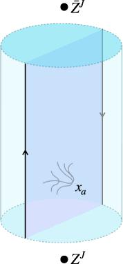
a. AdS₅

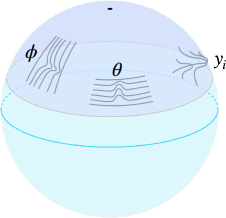
b. $S^{5}$

Figure 3: A qualitative sketch of the four types of bosonic fluctuations of the semiclassical string dual to the Wilson line with $Z^{J}$ and $\bar{Z}^{J}$. In the static gauge, there are a. $3$ fluctuation modes, labelled $x^{a}$, orthogonal to the AdS₂ strip formed by the classical string in AdS₅, and b. $1+1+3$ fluctuation modes, labelled $\phi$, $\theta$ and $y^{i}$, in the azimuthal, polar and orthogonal directions of the $S^{2}$ partially wrapped by the classical string in $S^{5}$.

To summarize, (3.22) is our final result for the quadratic action of fluctuations in the static gauge. The eight transverse bosonic modes $x^{a}$, $y^{i}$, $\theta$ and $\phi$, which are schematically depicted in Figure 3, can be viewed as fields propagating on an asymptotically AdS₂ background, where the deformation from AdS₂ corresponds to turning on the non-zero angular momentum. Note that there is a manifest $SO(3)\times SO(3)_{R}$ symmetry rotating the $x$ and $y$ coordinates, and the $x$, $y$ and $\theta/\phi$ coordinates are decoupled to this order.

Let us finally remark that the expansion to quadratic order around a generic classical string solution in AdS${}_{5}\times S^{5}$ was discussed using a rather general formalism in [60] (see also [61]), working with the Polyakov action. We have checked that the results given in [60] precisely agree with (3.23), (3.24) and (3.26)-(3.28).

Bulk-to-bulk propagators.

The bulk-to-bulk propagators for the fluctuation modes, $G_{yy}$, $G_{xx}$, $G_{\theta\theta}=G_{\phi\phi}$ and $G_{\phi\theta}=-G_{\theta\phi}$, satisfy Green’s equations that follow from the quadratic action. For the $x$ and $y$ modes, they are

$$\left[\frac{1}{\sqrt{\gamma}}\partial_{\mu}\left(\sqrt{\gamma}\gamma^{\mu\nu}\partial_{\nu}\right)-m_{x}^{2}(\rho)\right]G_{xx}(\rho,\tau;\rho^{\prime},\tau^{\prime}) =-\frac{1}{2g\sqrt{\gamma}}\delta(\rho-\rho^{\prime})\delta(\tau-\tau^{\prime}),$$ (3.29)

$$\left[\frac{1}{\sqrt{\gamma}}\partial_{\mu}\left(\sqrt{\gamma}\gamma^{\mu\nu}\partial_{\nu}\right)-m_{y}^{2}(\rho)\right]G_{yy}(\rho,\tau;\rho^{\prime},\tau^{\prime}) =-\frac{1}{2g\sqrt{\gamma}}\delta(\rho-\rho^{\prime})\delta(\tau-\tau^{\prime}).$$ (3.30)

Meanwhile, since the $\theta$ and $\phi$ modes are coupled in the Lagrangian in (3.26), the corresponding bulk-to-bulk propagators satisfy coupled Green’s equations:

$$\left[\frac{1}{\sqrt{\gamma}}\partial_{\mu}\left(\sqrt{\gamma}\gamma^{\mu\nu}\partial_{\nu}\right)-m_{\theta\phi}^{2}(\rho)\right]G_{\theta\theta}+2is(\rho)\partial_{\tau}G_{\phi\theta} =-\frac{1}{2g\sqrt{\gamma}}\delta(\rho-\rho^{\prime})\delta(\tau-\tau^{\prime}),$$ (3.31)

$$\left[\frac{1}{\sqrt{\gamma}}\partial_{\mu}\left(\sqrt{\gamma}\gamma^{\mu\nu}\partial_{\nu}\right)-m_{\theta\phi}^{2}(\rho)\right]G_{\phi\theta}-2is(\rho)\partial_{\tau}G_{\theta\theta} =0.$$ (3.32)

These equations are accompanied by the boundary condition that each propagator vanishes at both boundaries of the strip: $G(\rho,\tau;\rho^{\prime},\tau^{\prime})\to 0$ as $\rho\to\pm\infty$. The normalization of the delta function on the RHS of (3.29)-(3.31) makes it explicit that the bulk-to-bulk propagators scale with the inverse of the string tension.

The propagators have a number of useful symmetries that follow either from the quadratic action or the Green’s equations. First, $G_{xx}$, $G_{yy}$ and $G_{\theta\theta}$ are all real, even under interchange of the bulk points (e.g., $G_{xx}(\rho,\tau;\rho^{\prime},\tau^{\prime})=G_{xx}(\rho^{\prime},\tau^{\prime};\rho,\tau)$), even under parity (e.g., $G_{xx}(\rho,\tau;\rho^{\prime},\tau^{\prime})=G_{xx}(-\rho,\tau;-\rho^{\prime},\tau^{\prime})=G_{xx}(\rho,-\tau;\rho^{\prime},-\tau^{\prime})$), and invariant under translations along $\tau$ (e.g., $G_{xx}(\rho,\tau;\rho^{\prime},\tau^{\prime})=G_{xx}(\rho,\tau+a;\rho^{\prime},\tau^{\prime}+a)$ for any $a\in\mathbb{R}$). By contrast, while $G_{\phi\theta}$ is also invariant under translations along $\tau$ and even under $\rho,\rho^{\prime}\to-\rho,-\rho^{\prime}$, it is imaginary, odd under interchange of the bulk points, and odd under $\tau,\tau^{\prime}\to-\tau,-\tau^{\prime}$. The difference in behavior of $G_{\phi\theta}$ can be traced to the $is\partial_{\tau}$ terms in (3.31) and (3.32).

From global to Poincaré coordinates.

So far we have studied the fluctuations of the dual string using coordinates on AdS${}_{5}\times S^{5}$ in which the AdS₂ slices are parametrized by the global coordinates, $\rho,\tau$. In these coordinates, the translational symmetry of the classical string is manifest. However, Poincaré coordinates are perhaps a more familiar choice for stating the AdS/CFT dictionary between the defect four-point correlators in (2.19)-(2.22) and the bulk-to-bulk propagators and classical vertex operators. Thus, we will also parametrize the AdS₂ slices using Poincaré coordinates $t,z$ that are related to the global coordinates by

$$t+iz \equiv\frac{e^{\tau}(\tanh{\rho}\pm i\mathop{\rm sech}\nolimits{\rho})t_{4}+t_{3}}{e^{\tau}(\tanh{\rho}\pm i\mathop{\rm sech}\nolimits{\rho})+1}.$$ (3.33)

We take the upper sign if $t_{3}<t_{4}$ and the lower sign if $t_{3}>t_{4}$ so that $z\geq 0$. Going forward we assume $t_{3}<t_{4}$. The transformation indeed satisfies $d\rho^{2}+\cosh^{2}{\rho}d\tau^{2}=\frac{1}{z^{2}}(dt^{2}+dz^{2})$.

Two properties of (3.33) are worth noting: Firstly, $Z^{J}$ and $\bar{Z}^{J}$ are located at $t_{3}$ and $t_{4}$, respectively, on the AdS₂ boundary in accordance with (2.19)-(2.22). This follows from sending $\tau\to-\infty$ and $\tau\to\infty$ in (3.33). Secondly, to send the bulk point $\rho,\tau$ to the boundary point $t$, we

$$\text{fix }\tau =\log\left|\frac{t-t_{3}}{t_{4}-t}\right|, \text{and send }\rho \to\eta\infty$$ (3.34)

where $\eta=1$ if $t_{3}<t<t_{4}$ and $\eta=-1$ otherwise. In this limit, $z$ is asymptotically

$$z\sim\frac{2|t_{4}-t||t_{3}-t|}{t_{4}-t_{3}}e^{-\eta\rho}.$$ (3.35)

3.3 Four-point functions as boundary-to-boundary propagators

We are now ready to state the precise dictionary between the defect correlators on the Wilson line and the propagators on the classical string.

First, we identify the fluctuation modes dual to the elementary insertions introduced in Section 2. The six scalars, $\Phi_{I}$, in $\mathcal{N}=4$ SYM are dual to the $S^{5}$ embedding coordinates, $Y_{I}$. In particular, in the dCFT the $\Phi_{i}$, $i=1,2,3$, appearing in (2.19) are dual to $Y_{i}$, while $Z$ and $\bar{Z}$ are dual to $Y_{4}+iY_{5}=\sin{\bar{\theta}}e^{i\bar{\phi}}$ and $Y_{4}-iY_{5}=\sin{\bar{\theta}}e^{-i\bar{\phi}}$, respectively. Let us recall that the holographic correlators depend only on the asymptotic behavior of the fluctuation fields near the worldsheet boundary (see, e.g., (3.1)-(3.2)). Thus, given that $y_{i}\to 0$, $\bar{\theta}\to\bar{\theta}_{\rm cl}\to 1$ and $f_{y}\to 1$ as $\rho\to\pm\infty$, it follows from (3.11) and (3.20) that $Y_{i}\sim y_{i}$ asymptotically. We may therefore equivalently take the fluctuation field dual to $\Phi_{i}$ to be $y_{i}$. Indeed, as can be seen from the Lagrangian in (3.24), the $y_{i}$ have an $SO(3)\subset SO(6)$ rotational symmetry and their masses asymptotically satisfy $m_{y}^{2}\to 0$ as $\rho\to\pm\infty$, whose dual statements in the dCFT are that the scalars $\Phi_{i}$ preserve an $SO(3)\subset SO(6)$ R-symmetry and have scaling dimension $\Delta=1$. We will also shortly discuss what the string observables look like when the fields dual to $Z$ and $\bar{Z}$ are expressed in terms of $\theta$ and $\phi$, which are related to $\bar{\theta}$ and $\bar{\phi}$ by the field redefinitions in (3.20). For now we note that the masses of the $\theta$ and $\phi$ fields satisfy $m_{\theta\phi}^{2}\to 0$ asymptotically near the boundary (see (3.28)), which matches the fact that $Z$ and $\bar{Z}$ have scaling dimension $\Delta=1$. Finally, the displacement operators $\mathbb{D}_{a}$ are dual to the AdS₅ embedding coordinates, $X_{a}$, $a=1,2,3$, that are transverse to the Wilson line on the boundary. Again because $x_{a}\to 0$ as $\rho\to\pm\infty$, it follows from (3.10) that $X_{a}\sim x_{a}$ asymptotically and therefore we may equivalently take the fluctuation field dual to $\mathbb{D}_{a}$ to be $x_{a}$. Indeed, as can be seen from the Lagrangian in (3.23), the $x_{a}$ have an $SO(3)$ symmetry of rotations in AdS₅ about the classical string and their masses satisfy $m_{x}^{2}\to 2$ as $\rho\to\pm\infty$, whose dual statements in the dCFT are that the $\mathbb{D}_{a}$ have an $SO(3)$ symmetry of rotations in $\mathbb{R}^{4}$ about the Wilson line and have scaling dimension $\Delta=2$.

The vertex operators dual to $\Phi_{i}$, $\mathbb{D}_{a}$, $Z$ and $\bar{Z}$ are therefore:

$$v_{\Phi_{i}}(t) \equiv\lim_{z\to 0}\frac{2g}{z}y_{i}(z,t), v_{\mathbb{D}_{a}}(t) \equiv\lim_{z\to 0}\frac{2g}{z^{2}}x_{a}(z,t),$$ (3.36)

$$v_{Z}(t) \equiv\lim_{z\to 0}\frac{2g}{z}\sin(\bar{\theta}(z,t))e^{i\bar{\phi}(z,t)}, v_{\bar{Z}}(t) \equiv\lim_{z\to 0}\frac{2g}{z}\sin(\bar{\theta}(z,t))e^{-i\bar{\phi}(z,t)}.$$ (3.37)

This makes (3.2) precise. Although the above vertex operators are defined using Poincaré coordinates, we will take advantage of the simplicity of the classical string in global coordinates and take the bulk-to-boundary limits using (3.34) and (3.35).

Given (3.14), the vertex operators on the classical solution simplify to:

$$v_{\Phi_{i}}\rvert_{\Psi_{\rm cl}} =v_{\mathbb{D}_{a}}\rvert_{\Psi_{\rm cl}}=0, v_{Z}(t)\rvert_{\Psi_{\rm cl}} =2gce^{i\phi_{0}}\frac{t_{4}-t_{3}}{(t_{4}-t)^{2}}, v_{\bar{Z}}(t)\rvert_{\Psi_{\rm cl}} =2gce^{-i\phi_{0}}\frac{t_{4}-t_{3}}{(t_{3}-t)^{2}}.$$ (3.38)

These expressions for the classical vertex operators, which determine the leading large charge behavior of the defect correlators consisting of powers of $Z$ and $\bar{Z}$ in the background of $Z^{J}$ and $\bar{Z}^{J}$, are familiar from [41]. Meanwhile, the subleading large charge behavior due to the quadratic fluctuations about the classical solution are determined by sending the endpoints of the bulk-to-bulk propagators to the boundary as outlined in (3.5)-(3.7). In particular, given that the vertex operators dual to $\Phi_{i}$ and $\mathbb{D}_{a}$ are zero on the classical solution, the leading contribution to the defect correlators in (2.19) and (2.22) are given by

$$\frac{\braket{\Phi_{i}(t_{1})\Phi_{j}(t_{2})Z^{J}(t_{3})\bar{Z}^{J}(t_{4})}}{\braket{Z^{J}(t_{3})\bar{Z}^{J}(t_{4})}} =W_{yy}(t_{1},t_{2})\delta_{ij},$$ (3.39)

$$\frac{\braket{\mathbb{D}_{a}(t_{1})\mathbb{D}_{b}(t_{2})Z^{J}(t_{3})\bar{Z}^{J}(t_{4})}}{\braket{Z^{J}(t_{3})\bar{Z}^{J}(t_{4})}} =W_{xx}(t_{1},t_{2})\delta_{ab},$$ (3.40)

where the boundary-to-boundary propagator $W$ ($\equiv W_{yy},W_{xx}$) is related to the bulk-to-bulk propagator $G$ ($\equiv G_{yy},G_{xx}$) by

$$W(t_{1},t_{2}) \equiv(2\Delta-1)^{2}\lim_{\begin{subarray}{c}z_{1}\to 0^{+}\\ z_{2}\to 0^{+}\end{subarray}}\frac{2g}{z_{1}^{\Delta}}\frac{2g}{z_{2}^{\Delta}}G(t_{1},z_{1};t_{2},z_{2})$$

$$=\frac{(2\Delta-1)^{2}}{2^{2\Delta-2}}\frac{g^{2}}{t_{12}^{2\Delta}}\frac{\chi^{2\Delta}}{|1-\chi|^{\Delta}}\lim_{\begin{subarray}{c}\rho\to\eta_{1}\infty\\ \rho^{\prime}\to\eta_{2}\infty\end{subarray}}e^{\eta_{1}\Delta\rho}e^{\eta_{2}\Delta\rho^{\prime}}G(\rho,\tau(t_{1});\rho^{\prime},\tau(t_{2})).$$ (3.41)

In the second line, we have sent the bulk point to the boundary in accordance with (3.34) (see Figure 4) and written the ratios of distances on the Wilson line coming from (3.35) in terms of the conformal ratio $\chi$ defined in (2.15). Because of the translational symmetry along $\tau$, $G$ depends only on the difference between $\tau(t_{1})$ and $\tau(t_{2})$, which reduces to

$$\tau(t_{1})-\tau(t_{2})=\log\left|\frac{t_{13}}{t_{14}}\frac{t_{24}}{t_{23}}\right|=-\log|1-\chi|.$$ (3.42)

Thus, the boundary-to-boundary propagator has the same conformal form as the defect correlators in (2.19)-(2.22).

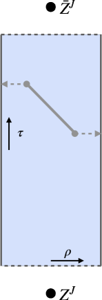
a.

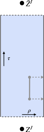
b.

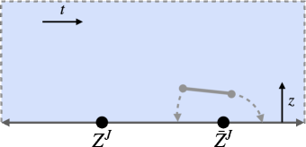
c.

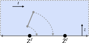
d.

Figure 4: Sending the endpoints of the bulk-to-bulk propagators to the boundary in global (a. and b.) and in Poincaré (c. and d.) coordinates, in accordance with (3.34). When the bulk points are sent to opposite boundaries in global coordinates, as in a., the light insertions on the Wilson line are separated by the heavy insertions, as in c.. In this case $\chi>1$. When the bulk points are sent to the same boundary in global coordinates, as in b., the light insertions are between the two heavy insertions, as in d.. In this case $\chi<1$.

Finally, we express the vertex operators dual to the light insertions $Z$ and $\bar{Z}$ in terms of the rescaled fluctuation fields $\theta$ and $\phi$. We begin by expanding $v_{Z}$ in (3.37) to linear order in $\theta$ and $\phi$:

$$v_{Z}(t) =\lim_{z\to 0}\frac{2g}{z}\left[\sin{\theta_{\rm cl}}e^{i\phi_{\rm cl}}+\frac{\cos{\theta_{\rm cl}}}{f_{\theta}}e^{i\phi_{\rm cl}}\theta+i\frac{\sin{\theta_{\rm cl}}}{f_{\phi}}e^{i\phi_{\rm cl}}\phi+\ldots\right]$$

$$=v_{Z}(t)\rvert_{\Phi_{\rm cl}}+e^{\tau(t)+i\phi_{0}}\lim_{z\to 0}\frac{2g}{z}\left(\theta+i\phi\right)+\ldots.$$ (3.43)

To get to the second line, we used that $\cos{\theta_{\rm cl}}/f_{\theta}\to 1$ and $\sin{\theta_{\rm cl}}/f_{\phi}\to 1$ as $\rho\to\pm\infty$, which follow from (3.14) and (3.21). Likewise, $v_{\bar{Z}}$ in (3.37) expanded to linear order is

$$v_{\bar{Z}}(t) =v_{\bar{Z}}(t)\rvert_{\Psi_{\rm cl}}+e^{-\tau(t)-i\phi_{0}}\lim_{z\to 0}\frac{2g}{z}\left(\theta-i\phi\right)+\ldots.$$ (3.44)

Thus, the holographic expression for the leading and first subleading terms in the large charge expansion of the defect correlators in (2.20)-(2.21) is:

$$\frac{\braket{Z(t_{1})\bar{Z}(t_{2})Z^{J}(t_{3})\bar{Z}^{J}(t_{4})}}{\braket{Z^{J}(t_{3})\bar{Z}^{J}(t_{4})}} =v_{Z}(t_{1})\rvert_{\Psi_{\rm cl}}v_{\bar{Z}}(t_{2})\rvert_{\Psi_{\rm cl}}+2e^{\tau(t_{1})-\tau(t_{2})}(W_{\theta\theta}(t_{1},t_{2})+iW_{\phi\theta}(t_{1},t_{2})),$$ (3.45)

$$\frac{\braket{\bar{Z}(t_{1})Z(t_{2})Z^{J}(t_{3})\bar{Z}^{J}(t_{4})}}{\braket{Z^{J}(t_{3})\bar{Z}^{J}(t_{4})}} =v_{\bar{Z}}(t_{1})\rvert_{\Psi_{\rm cl}}v_{Z}(t_{2})\rvert_{\Psi_{\rm cl}}+2e^{\tau(t_{2})-\tau(t_{1})}(W_{\theta\theta}(t_{1},t_{2})-iW_{\phi\theta}(t_{1},t_{2})),$$ (3.46)

where the boundary-to-boundary propagator $W$ ($\equiv W_{\theta\theta},W_{\phi\theta}$) is again given in terms of the bulk-to-bulk propagator $G$ ($\equiv G_{\theta\theta},G_{\phi\theta}$) by (3.3) with $\Delta=1$.

Finally, we note from (3.38) that the classical pieces in (3.45)-(3.46) are explicitly:

$$v_{Z}(t_{1})\rvert_{\Psi_{\rm cl}}v_{\bar{Z}}(t_{2})\rvert_{\Psi_{\rm cl}} =\frac{4g^{2}c^{2}}{t_{12}^{2}}\frac{\chi^{2}}{(1-\chi)^{2}}, v_{\bar{Z}}(t_{1})\rvert_{\Psi_{\rm cl}}v_{Z}(t_{2})\rvert_{\Psi_{\rm cl}} =\frac{4g^{2}c^{2}}{t_{12}^{2}}\chi^{2}.$$ (3.47)

4 Computing the Green’s functions

The last step in determining the defect four-point correlators is to compute the boundary-to-boundary propagators. We begin by presenting a general way to express the bulk propagators as integrals over Fourier modes conjugate to the global boundary coordinate, send the bulk points to the boundary, and rewrite the resulting integral representation of the boundary propagator as a series. We then apply the procedure to first compute $W_{yy}$, which lets us determine $W_{\theta\theta}$ and $W_{\theta\phi}$ via the superconformal Ward identities, and then compute $W_{xx}$.

4.1 Integral and series representations of the propagators

Taking advantage of the symmetry of the classical string in (3.14) under translations in the global time coordinate $\tau$, we write the $yy$ and $xx$ bulk-to-bulk propagators in their Fourier representations:

$$G(\rho,\tau;\rho^{\prime},\tau^{\prime})\equiv\frac{1}{4\pi g}\int_{-\infty}^{\infty}dke^{ik(\tau-\tau^{\prime})}g(\rho,\rho^{\prime};k).$$ (4.1)

Here, $G\equiv G_{yy}$ and $g(\rho,\rho^{\prime};k)\equiv g_{yy}(\rho,\rho^{\prime};k)$ or $G\equiv G_{xx}$ and $g(\rho,\rho^{\prime};k)\equiv g_{xx}(\rho,\rho^{\prime};k)$.

Noting the explicit form of the d’Alembertian on the classical string worldsheet in global coordinates,

$$\partial_{\mu}\left(\sqrt{\gamma}\gamma^{\mu\nu}\partial_{\nu}\right)=\frac{\partial}{\partial\rho}\left(\sqrt{\cosh^{2}{\rho}-c^{2}}\frac{\partial}{\partial\rho}\right)+\frac{1}{\sqrt{\cosh^{2}{\rho}-c^{2}}}\frac{\partial^{2}}{\partial\tau^{2}},$$ (4.2)

and substituting the Fourier representations of $G_{yy}$ and $G_{xx}$ into (3.30) and (3.29), we find that $g_{yy}$ and $g_{xx}$ satisfy

$$\left(\frac{d}{d\rho}\left(\sqrt{\cosh^{2}{\rho}-c^{2}}\frac{d}{d\rho}\right)-\frac{k^{2}}{\sqrt{\cosh^{2}{\rho}-c^{2}}}-\sqrt{\gamma}m^{2}(\rho)\right)g(\rho,\rho^{\prime};k)=-\delta(\rho-\rho^{\prime}),$$ (4.3)

where $m^{2}\equiv m_{y}^{2}$ or $m^{2}\equiv m_{x}^{2}$, as appropriate. We additionally impose the boundary condition $g(\rho,\rho^{\prime};k)\to 0$ as $\rho\to\pm\infty$, which gives the standard asymptotic behavior $g\sim e^{\mp\Delta\rho}$. We also note the symmetries of $g$: $g(\rho,\rho^{\prime};k)=g(\rho^{\prime},\rho;k)=g(-\rho,-\rho^{\prime};k)=g(\rho,\rho^{\prime};-k)$. These properties follow from (4.3) and/or the discussion after (3.32). It follows that $G$ only depends on $\tau$ and $\tau^{\prime}$ through the combination $|\tau-\tau^{\prime}|$.

The equation for $g(\rho,\rho^{\prime};k)$ simplifies if we change variables from $\rho$ to the compactified coordinate

$$r\equiv\int_{0}^{\rho}\frac{\sqrt{1-c^{2}}d\rho^{\prime}}{\sqrt{\cosh^{2}{\rho^{\prime}}-c^{2}}}=-i\mathbb{F}\left(i\rho\Big{\rvert}\frac{1}{1-c^{2}}\right),$$ (4.4)

where $\mathbb{F}(x|m)$ is the incomplete elliptic integral of the first kind. Equivalently, $\cosh{\rho}=\text{cn}\left(ir|\frac{1}{1-c^{2}}\right)$, where $\text{cn}(x|m)$ is the Jacobi elliptic function. The asymptotic behavior of $r$ as $\rho\to\pm\infty$ will play an important role in what follows. It is given by

$$r \sim\pm\left(r_{m}+\bar{r}_{m}e^{\mp\rho}+O(e^{\mp 2\rho})\right), \text{where }r_{m}\equiv\sqrt{1-c^{2}}\mathbb{K}(c^{2})\text{ and }\bar{r}_{m}\equiv-2\sqrt{1-c^{2}}.$$ (4.5)

Note that the change of variables in (4.4) is essentially the one that puts the induced metric (3.16) in the conformal gauge form (up to rescaling by a constant factor).

After the change of variables, (4.3) becomes

$$\left(\frac{d^{2}}{dr^{2}}-\frac{k^{2}}{1-c^{2}}-\frac{\sqrt{\cosh^{2}{\rho}-c^{2}}\sqrt{\gamma}m^{2}}{1-c^{2}}\biggr{\rvert}_{\cosh{\rho}\to\text{cn}\left(ir|\frac{1}{1-c^{2}}\right)}\right)g(r,r^{\prime};k) =-\frac{\delta(r-r^{\prime})}{\sqrt{1-c^{2}}}.$$ (4.6)

The solution to (4.6) may be written in the following piece-wise form:

$$g(r,r^{\prime};k)\equiv a(k)\left[g^{R}(r;k)g^{L}(r^{\prime};k)\theta(r-r^{\prime})+g^{L}(r;k)g^{R}(r^{\prime};k)\theta(r^{\prime}-r)\right].$$ (4.7)

Here, $g^{L}$ and $g^{R}$ solve (4.6) without the delta source term and satisfy the boundary conditions $g^{R}\to 0$ as $r\to r_{m}$ and $g^{L}\to 0$ as $r\to-r_{m}$. The normalization $a(k)$ is fixed by needing to reproduce the prefactor of the delta function in (4.6):

$$a(k) \equiv-\frac{1}{\sqrt{1-c^{2}}}\left(\frac{dg^{R}(r;k)}{dr}g^{L}(r;k)-\frac{dg^{L}(r;k)}{dr}g^{R}(r;k)\right)^{-1}.$$ (4.8)

The explicit forms of the homogeneous differential equations that $g^{L}$ and $g^{R}$ solve for the two different fluctuation modes are:

$$\left(-\frac{d^{2}}{dr^{2}}+\frac{2c^{2}}{1-c^{2}}\text{cn}\left(ir|\frac{1}{1-c^{2}}\right)^{-2}\right)g^{L/R}_{yy}(r;k) =\frac{c^{2}-k^{2}}{1-c^{2}}g_{yy}^{L/R}(r;k),$$ (4.9)

$$\left(-\frac{d^{2}}{dr^{2}}+\frac{2}{1-c^{2}}\text{cn}\left(ir|\frac{1}{1-c^{2}}\right)^{2}\right)g^{L/R}_{xx}(r;k) =\frac{c^{2}-k^{2}}{1-c^{2}}g_{xx}^{L/R}(r;k).$$ (4.10)

We can always choose $g^{L}$ and $g^{R}$ to satisfy

$$g^{R}(r;k)=g^{R}(r;-k)=g^{L}(-r;k).$$ (4.11)

The second equality can be imposed because the masses are even under $\rho\to-\rho$ or, equivalently, $\text{cn}(ir|\frac{1}{1-c^{2}})$ is even under $r\to-r$. Finally, we note that the boundary conditions impose the following asymptotic behavior:

$$g^{R}\sim(r-r_{m})^{\Delta}\hskip 14.22636pt\text{as }r\to r_{m}, g^{L}\sim(r+r_{m})^{\Delta}\hskip 14.22636pt\text{as }r\to-r_{m}.$$ (4.12)

Eq. (4.1) and (4.7) give an explicit integral representation for the $G_{xx}$ and $G_{yy}$ in terms of solutions to the ODEs in (4.9)-(4.10). The next step is to convert the integral in (4.1) into a sum of residues. First, we replace $\tau-\tau^{\prime}$ by $|\tau-\tau^{\prime}|$ in (4.1) (see the comment below (4.3)) and close the contour in the upper half-plane. There is no contribution from the arc at infinity because of the $e^{ik|\tau-\tau^{\prime}|}$ term as long as $\tau\neq\tau^{\prime}$. Next, we note that $g(r,r^{\prime};k)$ has poles where $1/a(k)$, the Wronskian of $g^{R}(r;k)$ and $g^{L}(r;k)$, is zero. For these values of $k$, $g^{R}$ and $g^{L}$ are linearly dependent and define a single solution that vanishes at both $r=r_{m}$ and $r=-r_{m}$. Eqs. (4.9) and (4.10) take the form of the time-independent Schrödinger equation with real potentials $V_{y}(r)\equiv\frac{2c^{2}}{1-c^{2}}\text{cn}\left(ir\rvert\frac{1}{1-c^{2}}\right)^{-2}$ and $V_{x}(r)\equiv\frac{2}{1-c^{2}}\text{cn}\left(ir\rvert\frac{1}{1-c^{2}}\right)^{2}$ (and $\hbar^{2}/2/m=1$). Therefore, the solutions $g^{L}\propto g^{R}$ at the poles are naturally interpreted as bound states of a one-dimensional particle with energy $\mathcal{E}=\frac{c^{2}-k^{2}}{1-c^{2}}$ moving in a potential $V(r)$ ($\equiv V_{y}(r),V_{x}(r)$) with hard walls at $r=\pm r_{m}$ (because of the boundary conditions on $g^{R}$ and $g^{L}$). As we will verify explicitly in Sections 4.2 and 4.3, the poles of both $g_{yy}(\rho,\rho^{\prime};k)$ and $g_{xx}(\rho,\rho^{\prime};k)$ lie on the imaginary $k$ axis. Alternatively, this follows from the fact that the energy eigenvalues are necessarily real and obey the bound $\mathcal{E}>\frac{c^{2}}{1-c^{2}}$, which means the bound states only exist for $k^{2}<0$. The lower bound on $\mathcal{E}$ is obvious for $V_{x}(r)$, which attains the minimum value $\frac{2}{1-c^{2}}$ at $r=0$, and can be verified numerically for $V_{y}(r)$. The behavior of $g^{R}$ and $g^{L}$ at and away from the poles of $g(r,r;k)$ is illustrated in Figure 5.

Therefore, labelling the poles $k_{n}\in i\mathbb{R}^{+}$, $n=0,1,2,\ldots$, we can write the bulk-to-bulk propagator as

$$G(r,\tau;r^{\prime},\tau^{\prime})=\sum_{n=0}^{\infty}e^{ik_{n}|\tau-\tau^{\prime}|}\left(\frac{1}{4\pi g}\oint_{k_{n}}dk\text{ }a(k)\right)g^{R}(r;k_{n})g^{L}(r^{\prime};k_{n}).$$ (4.13)

We used (4.7) and the fact that $g^{R}(r;k_{n})g^{L}(r^{\prime};k_{n})=g^{L}(r;k_{n})g^{R}(r^{\prime};k_{n})$, which follows because $g^{L}\propto g^{R}$ at $k=k_{n}$. We have also assumed that the $k_{n}$ are simple poles of $g(r,r^{\prime};k)$, so we can evaluate $g^{R}$ and $g^{L}$ at $k_{n}$ and pull them out of the contour integral.

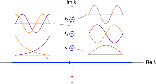
Figure 5: The contour in the Fourier integral representation of the bulk and boundary propagators runs along the real $k$ axis (shown in blue). We can close it at infinity in the upper half plane and pick up the residues at the poles, $k_{n}$, $n=0,1,2,\ldots$, along the positive imaginary $k$ axis. The insets sketch the solutions $g^{R}(r;k)$ (orange) and $g^{L}(r;k)$ (purple) at a few representative values of $k$, including at the poles ($k_{0}$, $k_{1}$ and $k_{2}$), on the imaginary axis away from the poles, and on the real axis.

To convert the series for the bulk-to-bulk propagator into a series for the boundary-to-boundary propagator, we send $\rho\to\eta_{1}\infty$ and $\rho^{\prime}\to\eta_{2}\infty$ (which sends $r\to\eta_{1}r_{m}$ and $r^{\prime}\to\eta_{2}r_{m}$) in accordance with (3.3). We can do so term-by-term in the series because each $g^{R}(r;k_{n})$ or $g^{L}(r;k_{n})$ vanishes at both $r=\pm r_{m}$ and combines with the divergent factor $e^{\eta\Delta\rho}$ to yield a finite result in terms of $k_{n}$. There are two distinct cases to consider: $\eta_{1}=\eta_{2}$, when the two bulk points approach the same boundary, and $\eta_{1}=-\eta_{2}$, when the two bulk points approach opposite boundaries. These two cases are related in a simple way, as we can see by again exploiting the analogy with the Schrödinger equation in one dimension. Because the parities of the energy eigenstates in an even potential alternate (with the ground state being even), it follows that $g^{R}(r;k_{n})=g^{L}(-r;k_{n})=(-1)^{n}g^{R}(-r;k_{n})$. Therefore,

$$\lim_{\rho\to\eta\infty}e^{\eta\Delta\rho}g^{R}(r(\rho);k_{n})=\lim_{\rho\to-\eta\infty}e^{-\eta\Delta\rho}g^{L}(r(\rho);k_{n})=\eta^{n}\lim_{\rho\to\infty}e^{\Delta\rho}g^{R}(r(\rho);k_{n}).$$ (4.14)

This is useful because it is easier in practice to evaluate the first limit on the LHS of (4.14) when $\eta=1$. This is because the limit of $e^{\Delta\rho}g^{R}(r(\rho);k)$ as $\rho\to\infty$ is finite for any $k$ while the limit as $\rho\to-\infty$ is finite only if $k=k_{n}$.

Combining (3.3) and (4.13), and applying (3.42) and (4.14), we finally arrive at the following series representation for the boundary-to-boundary propagator:

$$W(t_{1},t_{2}) =\frac{(2\Delta-1)^{2}}{2^{2\Delta-2}}\frac{g}{t_{12}^{2\Delta}}\frac{\chi^{2\Delta}}{|1-\chi|^{\Delta}}\sum_{n=0}^{\infty}\biggr{[}(-\eta_{1}\eta_{2})^{n}e^{ik_{n}|\log|1-\chi||}$$ (4.15)

$$\hskip 170.71652pt\times\left(\frac{1}{4\pi}\oint_{k_{n}}dka(k)\right)\left(\lim_{\rho\to\infty}e^{\Delta\rho}g^{R}(r(\rho);k_{n})\right)^{2}\biggr{]}.$$

Note that $\eta_{1}\eta_{2}=\text{sgn}(1-\chi)$.

It is also possible to send the bulk points to the boundary without writing the Fourier integral as a sum of residues. This is mainly useful if we can interchange the limit and the integral, which requires that the two bulk points be sent to opposite boundaries. For instance, if we first send $\rho\to\infty$ inside the integrand of (4.1), then the step function in (4.7) sets $g(r,r^{\prime};k)=a(k)g^{R}(r;k)g^{L}(r^{\prime};k)$ and we must subsequently send $\rho^{\prime}\to-\infty$ because $g^{L}(r^{\prime};k)$ does not vanish at $\rho^{\prime}\to\infty$ for real $k$. We find the following integral representation for the boundary-to-boundary propagator, which is valid when $\chi>1$:

$$W(t_{1},t_{2}) =\frac{(2\Delta-1)^{2}}{2^{2\Delta}\pi}\frac{g}{t_{12}^{2\Delta}}\frac{\chi^{2\Delta}}{(\chi-1)^{\Delta}}\int_{-\infty}^{\infty}dke^{ik\log(\chi-1)}a(k)\left(\lim_{\rho\to\infty}e^{\Delta\rho}g^{R}(r(\rho);k)\right)^{2}.$$ (4.16)

In certain cases, this representation is more useful than (4.15).

4.2 Computing $W_{yy}$, $W_{\theta\theta}$ and $W_{\phi\theta}$

We now implement the analysis developed in the previous section to find the boundary-to-boundary propagator $W_{yy}$. Via (3.39) and (2.19), this determines the leading large charge behavior of the defect correlator $\braket{\Phi\Phi Z^{J}\bar{Z}^{J}}/\braket{Z^{J}\bar{Z}^{J}}$ and of $G_{1}(\chi)$. Using the superconformal Ward identities, we will then also determine $G_{Z\bar{Z}}(\chi)$ and $G_{\bar{Z}Z}(\chi)$, which are equivalent to $W_{\theta\theta}$ and $W_{\phi\theta}$.

4.2.1 Computing $W_{yy}$

The key to computing $W_{yy}$ analytically is to recognize that (4.9) can be put in the Jacobi form of the Lamé differential equation. This ODE appeared previously in studies of one-loop corrections to the energies of “elliptic” classical strings in AdS${}_{5}\times S^{5}$ [62, 63, 64, 65]. We summarize the equation in Appendix A along with conventions and identities for the elliptic integrals, Jacobi elliptic functions, and the theta functions. These special functions appear prominently throughout this section.

In order to put (4.9) into the Jacobi form of the Lamé equation, we rewrite it in terms of the new coordinate

$$\sigma \equiv\frac{cr}{\sqrt{1-c^{2}}}+\mathbb{K}\left(\frac{1}{c^{2}}\right)+i\mathbb{K}\left(1-\frac{1}{c^{2}}\right).$$ (4.17)

Using the identities in (A.18)-(A.20) and (A.21)-(A.23), we can simplify (4.9) to

$$\left[-\partial_{\sigma}^{2}+\frac{2}{c^{2}}\text{sn}^{2}\left(\sigma|\frac{1}{c^{2}}\right)\right]g_{yy}^{R/L}(\sigma;k) =\left(1-\frac{k^{2}}{c^{2}}\right)g^{R/L}_{yy}(\sigma;k).$$ (4.18)

This matches the form of the Lamé equation given in (A.29), if we identify the parameter $m$ and the eigenvalue $\Lambda$ to be:

$$m \equiv\frac{1}{c^{2}}, \Lambda \equiv 1-\frac{k^{2}}{c^{2}}.$$ (4.19)

Because they are ubiquitous in the following discussion, it is convenient to introduce the following standard shorthand:

$$\mathbb{K} \equiv\mathbb{K}\left(\frac{1}{c^{2}}\right)=c\mathbb{K}(c^{2})-ic\mathbb{K}(1-c^{2}),$$ (4.20)

$$\mathbb{K}^{\prime} \equiv\mathbb{K}\left(1-\frac{1}{c^{2}}\right)=c\mathbb{K}(1-c^{2}).$$ (4.21)

The second way of writing $\mathbb{K}$ and $\mathbb{K}^{\prime}$ follows from (A.3)-(A.4). Since $\mathbb{K}(c^{2})$ and $\mathbb{K}(1-c^{2})$ are positive real numbers for $c^{2}\in(0,1)$, it follows that $\mathbb{K}^{\prime}$ and $\mathbb{K}+i\mathbb{K}^{\prime}$ are also positive real numbers, but $\mathbb{K}$ is complex. It will be convenient to work with $\mathbb{K}$ and $\mathbb{K}^{\prime}$ and convert to explicitly real expressions only at the end.

We also note that as $r$ runs from $-r_{m}$ to $r_{m}$, $\sigma$ in (4.17) runs from $\sigma_{-}$ to $\sigma_{+}$ along the real axis, where

$$\sigma_{-} \equiv 0, \sigma_{+} \equiv 2\mathbb{K}+2i\mathbb{K}^{\prime}.$$ (4.22)

As reviewed in Appendix A, the solutions to the Lamé equation are known in terms of theta functions. In particular, two linearly independent solutions to (4.18) are

$$f^{\pm}(\sigma;\alpha)\equiv\frac{H(\pm\sigma+\alpha|m)}{\Theta(\sigma|m)}e^{\mp\sigma Z(\alpha|m)}.$$ (4.23)

Here $H$, $\Theta$ and $Z$ are defined in (A.32), and $\alpha$ is related to $k$ by the transformation $\text{sn}\left(\alpha\bigr{\rvert}m\right)=\sqrt{1+k^{2}}$ or, equivalently,

$$k\equiv i\text{cn}\left(\alpha\rvert m\right).$$ (4.24)

Because the Jacobi elliptic functions are doubly periodic (see (A.11)), the $\alpha$ complex plane is an infinite cover of the $k$ complex plane. We will see that this means the argument in Section 4.1 allowing us to convert the integral representation of the boundary-to-boundary propagator into a series representation can essentially be replicated in the $\alpha$ plane, but with some modification. We will take the “fundamental unit cell” in the $\alpha$ plane to be the rectangle with vertices at $\alpha=0$, $\alpha=2\mathbb{K}+2i\mathbb{K}^{\prime}$, $\alpha=-2i\mathbb{K}^{\prime}$ and $\alpha=2\mathbb{K}$. A representative set of vertical and horizontal lines in the unit cell is depicted in Figure 6 a, and its image in the $k$ plane is depicted in Figure 6 b. The periodic placement of the other copies of the unit cell in the $\alpha$ plane is shown in Figure 7. In particular, it will be useful to note the pre-images of the real and positive imaginary axes of the $k$ plane in the $\alpha$ unit cell: As $k$ runs from $-\infty$ to $\infty$ along the real axis (see Figure 7 b), $\alpha$ runs along the line segment from $-i\mathbb{K}^{\prime}$ to $i\mathbb{K}^{\prime}+2\mathbb{K}$ (see Figure 7 a), and as $k$ runs from $0$ to $ci$ to $i$ to $i\infty$ along the imaginary axis (see Figure 7 b), $\alpha$ runs along the line segments from $\mathbb{K}$ to $\mathbb{K}+i\mathbb{K}^{\prime}$ to $0$ to $-i\mathbb{K}^{\prime}$ (see Figure 7 a).

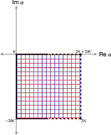
a. Fundamental unit cell in $\alpha$ plane

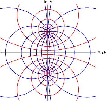
b. Image of fundamental unit cell in $k$ plane

Figure 6: To express the propagator $G_{yy}$ explicitly as a Fourier integral involving theta functions, we need to change the integration variable from $k$, the wavenumber conjugate to global time $\tau$, to $\alpha$ via (4.24). The $\alpha$ plane is an infinite cover of the $k$ plane. The fundamental unit cell in the $\alpha$ plane is depicted in a. and its image in the $k$ plane is depicted in b. Recall from (4.20)-(4.21) that $\mathbb{K}^{\prime}$ and $\mathbb{K}+i\mathbb{K}^{\prime}$ are real.

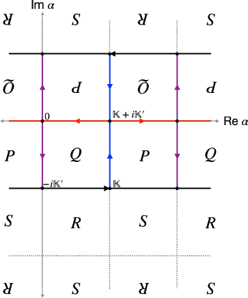
a. Periodicity of unit cells in $\alpha$ plane

b. Image of $\alpha$ unit cells in $k$ plane

Figure 7: The Jacobi elliptic function relating $k$ and $\alpha$ in (4.24) is doubly periodic, satisfying $\text{cn}\left(\alpha+2\mathbb{K}+2i\mathbb{K}^{\prime}\rvert m\right)=\text{cn}\left(\alpha\rvert m\right)$, $\text{cn}\left(\alpha+2i\mathbb{K}^{\prime}\rvert m\right)=-\text{cn}\left(\alpha\rvert m\right)$, as well as $\text{cn}\left(-\alpha\rvert m\right)=\text{cn}\left(\alpha\rvert m\right)$. Thus, the unit cells in the $\alpha$ plane are arranged as shown in a. Each grouping of four neighboring tiles labelled ‘Q’, ‘P’, ‘R’ and ‘S’, which are the pre-images of the four quadrants in the $k$ plane as shown in b., is one unit cell. The intervals $(-\infty,0)$ and $(0,\infty)$ on the real axis and $(0,ci)$, $(ci,i)$ and $(i,+\infty i)$ in the $k$ plane are indicated in b. using black, blue, red and purple directed line segments, respectively. Their pre-images in the $\alpha$ plane are likewise indicated in a.

Using (4.23), $g_{yy}^{R/L}$ can be written

$$g_{yy}^{R}(\sigma;\alpha) =\frac{f^{+}(\sigma;\alpha)}{f^{+}(\sigma_{+};\alpha)}-\frac{f^{-}(\sigma;\alpha)}{f^{-}(\sigma_{+};\alpha)},$$ (4.25)

$$g_{yy}^{L}(\sigma;\alpha) =\frac{f^{-}(\sigma;\alpha)}{f^{-}(\sigma_{-};\alpha)}-\frac{f^{+}(\sigma;\alpha)}{f^{+}(\sigma_{-};\alpha)}.$$ (4.26)

These manifestly satisfy the boundary conditions $g_{yy}^{R}(\sigma_{+};\alpha)=g_{yy}^{L}(\sigma_{-};\alpha)=0$. The parity and quasi-periodicity of the theta functions also imply that $g^{R/L}_{yy}(\sigma;\alpha)=g^{L/R}_{yy}(\sigma_{+}-\sigma;\alpha)$ and $g^{L/R}_{yy}(\sigma;\alpha+2\mathbb{K}a+2i\mathbb{K}^{\prime}b)=g^{L/R}_{yy}(\sigma;\alpha)$, for $a,b\in\mathbb{Z}$, which are analogous to (4.11).

Next, we compute the boundary limits of $g_{yy}^{R}(\sigma;\alpha)$ and $g_{yy}^{L}(\sigma;\alpha)$. First, we note the behavior of $\sigma$ near the end points, which follows from (4.5) and (4.17):

$$\sigma \sim\sigma_{\pm}\mp 2ce^{\mp\rho}, \text{ as }\rho \to\pm\infty.$$ (4.27)

Second, (4.12) implies that $g^{R}_{yy}\sim\sigma_{+}-\sigma$ as $\sigma\to\sigma_{+}$ and $g^{L}_{yy}\sim\sigma-\sigma_{-}$ as $\sigma\to\sigma_{-}$ (up to multiplicative factors independent of $\sigma$). Thus, we find:

$$\lim_{\rho\to\infty}e^{\rho}g_{yy}^{R}(\sigma;\alpha) =\lim_{\rho\to-\infty}e^{-\rho}g_{yy}^{L}(\sigma;\alpha)=-2c\frac{dg^{R}_{yy}}{d\sigma}\biggr{\rvert}_{\sigma=\sigma_{+}}=-4c(V(\alpha|m)-Z(\alpha|m)).$$ (4.28)

Here, $V(u|m)$ is defined in (A.33). Furthermore, the normalization becomes

$$\frac{1}{a_{yy}(\alpha)} =-c\frac{dg_{yy}^{R}(\sigma_{+};\alpha)}{d\sigma}g_{yy}^{L}(\sigma_{+};\alpha)=4c(V(\alpha|m)-Z(\alpha|m))\sinh\left(\frac{\pi i\alpha}{\mathbb{K}}+\sigma_{+}Z(\alpha|m)\right).$$ (4.29)

To simplify this result, we used the fact that $a_{yy}(\alpha)$ is independent of $\sigma$ to evaluate the Wronskian at $\sigma=\sigma_{+}$, a point at which $g_{yy}^{R}=0$ and $\frac{dg_{yy}^{R}}{d\sigma}$ is given by (4.28).

Using $\frac{dk}{d\alpha}=-i\text{sn}\left(\alpha|m\right)\text{dn}\left(\alpha|m\right)$ (note (4.24) and (A.14)) and (A.38) to express $V(\alpha|m)-Z(\alpha|m)$ in terms of the Jacobi elliptic functions, we can write the boundary limit of the bulk-to-bulk propagator as the following integral:

$$\lim_{\begin{subarray}{c}\rho\to\infty\\ \rho^{\prime}\to-\infty\end{subarray}}e^{\rho-\rho^{\prime}}G_{yy}(\rho,\tau;\rho^{\prime},\tau^{\prime})=-\frac{ci}{\pi g}\int_{-i\mathbb{K}^{\prime}}^{i\mathbb{K}^{\prime}+2\mathbb{K}}d\alpha\frac{\text{cn}\left(\alpha|m\right)\text{dn}^{2}\left(\alpha|m\right)\text{exp}\left(-\text{cn}\left(\alpha|m\right)|\tau-\tau^{\prime}|\right)}{\sinh\left(F(\alpha)\right)},$$ (4.30)

where

$$F(\alpha)\equiv\frac{\pi i\alpha}{\mathbb{K}}+2(\mathbb{K}+i\mathbb{K}^{\prime})Z(\alpha|m).$$ (4.31)

This is equivalent to (4.16) except we changed the integration variable from $k$ to $\alpha$.

The next step is to close the integration contour and pick up the residues at the poles. The integration contour in the $k$ plane can be closed using an arc at infinity, as in Figure 8 d, but the lifted contour in the $\alpha$ plane, shown in Figure 8 a, is not closed. However, the periodicity of the map from $\alpha$ to $k$, illustrated in Figure 7, allows us to close the lifted contour as in Figure 8 b at the cost of doubling the value of the integral. In particular, the contribution from the top horizontal segment duplicates the contribution from the bottom horizontal segment, while the contributions from the right and left vertical segments cancel. One can also see that the integral over the closed contour in the $\alpha$ plane is twice the original integral by noting the image of the the closed contour in the $k$ plane, which is given in Figure 8 e.

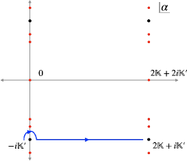
a.

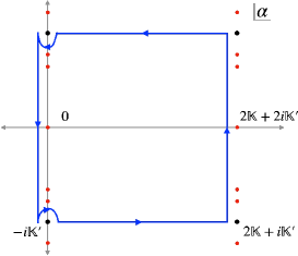
b.

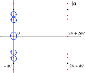
c.

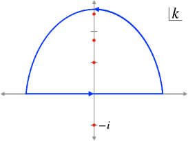
d.

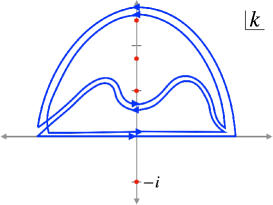
e.

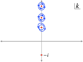
f.

Figure 8: Closing the integration contour in (4.30) and picking up the residues in both the $\alpha$ plane (a. - c.) and the $k$ plane (d. - f.). In d., the integration contour along the real axis in the $k$ plane is closed with an arc at infinity. The lift of this closed contour to the $\alpha$ plane via the map in (4.24) is not closed (a.). Using the periodic identification of the $\alpha$ plane (see Figure 7), the contour can be closed as in b. at the cost of doubling the integral. The doubling is clear from the image of the new contour in the $k$ plane (e.). Finally, in the $\alpha$ plane we can pick up the residues of the poles on the interval $[-i\mathbb{K}^{\prime},i\mathbb{K}^{\prime}]$ along the imaginary axis (c.). This corresponds to picking up two copies of the residues along the positive imaginary axis in the $k$ plane (f.).

To complete the argument, we need to identify the poles of the integrand of (4.30) that lie inside the closed contour. The poles of $\text{cn}(\alpha|m)$ and $\text{dn}(\alpha|m)$, which are at $\alpha=i\mathbb{K}^{\prime}+2a\mathbb{K}+2bi\mathbb{K}^{\prime}$, $a,b\in\mathbb{Z}$, all lie outside the contour. Thus, the only poles that contribute are the zeros of $\sinh\left(F(\alpha)\right)$ located inside the contour, which lie on the imaginary axis between $-i\mathbb{K}^{\prime}$ and $i\mathbb{K}^{\prime}$. We denote them $\alpha_{n}$, $n\in\mathbb{Z}$, and they satisfy

$$F(\alpha_{n})=n\pi i.$$ (4.32)

Because $Z(z|m)$ is odd, $\alpha_{0}=0$ and $\alpha_{-n}=-\alpha_{n}$.

The result of deforming the contour to individually encircle the poles at each $\alpha_{n}$ is depicted in Figure 8 c, and its image in the $k$ plane is depicted in Figure 8 f. Note that each pole in Figure 8 c is encircled once while each pole in Figure 8 f is encircled twice. This is because $\alpha_{n}$ and $\alpha_{-n}$ for $n>0$ are mapped to the same point in the $k$ plane, so the contours individually encircling the two poles in the $\alpha$ plane are mapped to two contours encircling the same pole in the $k$ plane. Meanwhile, the pole at $\alpha_{0}=0$ is special: because the map in (4.24) is even and therefore identifies points positioned antipodally with respect to the origin in the $\alpha$ plane, the image of the closed loop encircling $\alpha=0$ with winding number $1$ is a closed loop encircling $k=i$ with winding number $2$.

In order to evaluate the residues of (4.30) at $\alpha_{n}$, it is convenient to note the following elementary result: If $f(z)$ and $g(z)$ are analytic at $z_{n}$, $f(z_{n})=n\pi i$, and $f^{\prime}(z_{n})\neq 0$, then

$$\frac{1}{2\pi i}\oint_{z_{n}}dz\text{ }\frac{g(z)}{\sinh\left(f(z)\right)} =(-1)^{n}\frac{g(z_{n})}{f^{\prime}(z_{n})}.$$ (4.33)

Applying this result, we find that (4.30) can be written as

$$\lim_{\begin{subarray}{c}\rho\to\infty\\ \rho^{\prime}\to-\infty\end{subarray}}e^{\rho-\rho^{\prime}}G(\rho,\tau;\rho^{\prime},\tau^{\prime}) =\frac{c}{g}\sum_{n=-\infty}^{\infty}(-1)^{n}\frac{\text{cn}\left(\alpha_{n}|m\right)\text{dn}^{2}\left(\alpha_{n}|m\right)\text{exp}\left(-\text{cn}\left(\alpha_{n}|m\right)|\tau-\tau^{\prime}|\right)}{F^{\prime}(\alpha_{n})}.$$ (4.34)

Conveniently, the identity (A.37) lets us write the derivative of $Z(\alpha|m)$, and therefore $F^{\prime}(\alpha)$, in terms of the Jacobi elliptic functions. Additionally, we can use (A.3)-(A.6) and (A.7) to express $\mathbb{K}$, $\mathbb{K}^{\prime}$, $\mathbb{E}(\frac{1}{c^{2}})$ in terms of $\mathbb{K}(c^{2})$ and $\mathbb{E}(c^{2})$, and we ultimately find

$$F^{\prime}(\alpha)=\frac{2}{c}\left((1-c^{2})\mathbb{K}(c^{2})-\mathbb{E}(c^{2})\right)+2c\mathbb{K}(c^{2})\text{dn}^{2}\left(\alpha|m\right).$$ (4.35)

Eq. (4.30) is the final integral representation and (4.35), supplemented with (4.32), is the final series representation for the boundary limit of $G_{yy}$ expressed in terms of the $\alpha$ variables. Both expressions are perhaps more transparent when written in terms of the original $k$ variables, which gets rid of the elliptic functions and recasts the quantization condition in (4.32) in a more friendly form.

We first rewrite (4.30). $F$ can be written as a function of $k$ using $F(k)=\pi i+\int_{0}^{k}dk\frac{d\alpha}{dk}F^{\prime}(\alpha)$, and noting (4.35). Furthermore, using (4.24) and the identities in (A.16)-(A.17), all of the elliptic functions can be expressed in terms of $k$. Ultimately, we find

$$W_{yy}(t_{1},t_{2}) =\frac{g}{\pi}\frac{1}{t_{12}^{2}}\frac{\chi^{2}}{\chi-1}\int_{-\infty}^{\infty}dk\frac{k\sqrt{1-c^{2}+k^{2}}\cos(k\log(\chi-1))}{\sqrt{1+k^{2}}\sinh\left(2\int_{0}^{k}d\ell\frac{\mathbb{K}(c^{2})\ell^{2}+\mathbb{E}(c^{2})}{\sqrt{1+\ell^{2}}\sqrt{1-c^{2}+\ell^{2}}}\right)}.$$ (4.36)

We used (3.3) to relate $W_{yy}$ to the boundary limit of $G_{yy}$. Eq. (4.36) is valid when $\chi>1$.

Next, we rewrite (4.34). We introduce the “fluctuation energies”:

$$E_{n}\equiv-ik_{n}\equiv\text{cn}\left(\alpha_{n}\rvert m\right),$$ (4.37)

which are defined implicitly via (4.32). Note that $E_{0}=1$ and $E_{-n}=E_{n}$. It is perhaps more illuminating to define the energies in terms of an integral quantization condition, which follows from writing (4.32) as $n\pi i=\int_{0}^{\alpha_{n}}d\alpha F^{\prime}(\alpha)=\int_{1}^{E_{n}}dE^{\prime}\frac{d\alpha}{dE^{\prime}}F^{\prime}(\alpha)$ and using (4.35) and the Jacobi elliptic function identities in (A.16)-(A.17) to simplify the result. This leads precisely to (2.27).

Again using (A.16)-(A.17) to express the elliptic functions in (4.34) in terms of $E_{n}$, we find that the boundary-to-boundary propagator finally reduces to:

$$W_{yy}(t_{1},t_{2}) =\frac{2g}{\pi}\frac{1}{t_{12}^{2}}\frac{\chi^{2}}{|1-\chi|}\sum_{n\in\mathbb{Z}}\text{sgn}(1-\chi)^{n}f(E_{n})e^{-E_{n}|\log|1-\chi||},$$ (4.38)

where $f(E)$ is given in (2.29). In (4.38), we have replaced $(-1)^{n}$ in (4.34) by $\text{sgn}(1-\chi)^{n}$ in accordance with the discussion around (4.14)-(4.15). Thus, the series representation in (4.38) is valid for both $\chi>1$ and $\chi<1$. Finally, $G_{1}(\chi)=\frac{\pi}{2g}t_{12}^{2}W_{yy}(t_{1},t_{2})$ leads to (2.30).

Remarks about $G_{1}(\chi)$.

Let us make a few remarks about the final result for $G_{1}(\chi)$. Firstly, because $E_{n}=E_{-n}$, the positive and negative terms in (4.38) can naturally be combined. In general, the $n=0$ term must be treated separately from the $n\geq 1$ terms. It is special both because $E_{0}=1$ is independent of $c^{2}$ (this corresponds to the fact that the lowest operator in the conformal block expansion of the scalar four-point functions is protected), and because $k_{0}$ is the only pole in the $k$ upper half plane that is mapped $1$-to-$1$ with its pre-image $\alpha_{0}$ in the $\alpha$ plane.

Secondly, as a test of our results, we can consider the behavior of the four-point functions when $c^{2}=J=0$, in which case there are no large charges on the Wilson line and the four-point functions reduce to two-point functions. (Likewise the classical string does not rotate in $S^{5}$ and the propagators for the $S^{5}$ and AdS₅ modes reduce to those of scalars with $m^{2}=0$ and $m^{2}=2$ on AdS₂). It follows in this case from (2.28) that $\rho(E)=1$ and $E_{n}=|n|+1$, and from (2.29) that $f(1)=1$ and $f(E)=\frac{E}{2}$ for $E>1$. Therefore, the series representation of $W_{yy}(t_{1},t_{2})$ from (4.38) becomes

$$W_{yy}(t_{1},t_{2}) =\frac{2g}{\pi}\frac{1}{t_{12}^{2}}\frac{\chi^{2}}{|1-\chi|}\sum_{n=0}^{\infty}\text{sgn}(1-\chi)^{n}(n+1)e^{-(n+1)|\log|1-\chi||}.$$ (4.39)

Given that $4\sum_{n=1}^{\infty}ne^{-nx}=\sinh^{-2}{\frac{x}{2}}$ and $4\sum_{n=1}^{\infty}(-1)^{n+1}ne^{-nx}=\cosh^{-2}{\frac{x}{2}}$, the series can be explicitly summed for any $\chi$. We arrive at the result

$$\braket{\Phi_{i}(t_{1})\Phi_{j}(t_{2})}=W_{yy}(t_{1},t_{2})\delta_{ij}=\frac{2g}{\pi}\frac{1}{t_{12}^{2}}\delta_{ij}.$$ (4.40)

This correctly reproduces the leading behavior of the scalar two-point function in (2.17).

Thirdly, (2.30) is a compact representation of a function defined piecewise on $\chi\in(-\infty,0)$, $\chi\in(0,1)$, $\chi\in(1,2)$ and $\chi\in(2,\infty)$. Unpacking the absolute values yields

$$G_{1}(\chi) =\theta(-\chi)G^{(-\infty,0)}_{1}(\chi)+\theta(\chi)\theta(1-\chi)G^{(0,1)}_{1}(\chi)$$

$$+\theta(\chi-1)\theta(2-\chi)G^{(1,2)}_{1}(\chi)+\theta(\chi-2)G^{(2,\infty)}_{1}(\chi),$$ (4.41)

where $\theta(b-x)\theta(a-x)$ is $1$ if $a<x<b$ and $0$ otherwise and $G_{1}^{I}(\chi)$ denotes the series representation of $G_{1}(\chi)$ on the interval $I\subset\mathbb{R}$. Explicitly, we have

$$G^{(-\infty,0)}_{1}(\chi) =\chi^{2}\sum_{n\in\mathbb{Z}}\frac{f(E_{n})}{(1-\chi)^{E_{n}+1}}, G_{1}^{(0,1)}(\chi) =\chi^{2}\sum_{n\in\mathbb{Z}}f(E_{n})(1-\chi)^{E_{n}-1},$$ (4.42)

$$G_{1}^{(1,2)}(\chi) =\chi^{2}\sum_{n\in\mathbb{Z}}(-1)^{n}f(E_{n})(\chi-1)^{E_{n}-1}, G_{1}^{(2,\infty)}(\chi) =\chi^{2}\sum_{n\in\mathbb{Z}}(-1)^{n}\frac{f(E_{n})}{(\chi-1)^{E_{n}+1}}.$$ (4.43)

From the discussion around Figure 2, one would expect $G_{1}$ to behave piecewise on $\chi\in(-\infty,0)$, $\chi\in(0,1)$ and $\chi\in(1,\infty)$. The apparently special role of $\chi=2$ in (4.2.1) is an artifact of the series representation. In particular, while the series representations $G_{1}^{(1,2)}(\chi)$ and $G_{1}^{(2,\infty)}(\chi)$ do not converge at $\chi=2$, the integral representation in (4.36) is perfectly smooth at $\chi=2$. This is related to the convergence of the OPE as we will discuss shortly.

Finally, we comment on how (2.30) is consistent with $G_{1}(\chi)\to 1$ as $\chi\to 0$, which is imposed by the OPE limit in which the two light operators (or the two heavy operators) approach each other (in this limit, the leading exchanged operator is the identity). As $\chi\to 0$, the exponentially damping term in (2.30) is turned off and the series diverges due to the “infinite tail” consisting of terms with arbitrarily large values of $n$. The contribution of the tail is captured by an integral over $E$ weighted by the energy density $\rho(E)$. Since large values of $E$ dominate, we may replace the energy density and form factor by their asymptotic forms: $\rho(E)\sim\frac{2\mathbb{K}(c^{2})}{\pi}$, $f(E)\sim\frac{\pi}{4}\frac{E}{\mathbb{K}(c^{2})}$. Thus, as $\chi\to 0$,

$$\sum_{n\in\mathbb{Z}}f(E_{n})e^{-E_{n}|\log(1-\chi)|} \sim\int_{E_{\rm cutoff}}^{\infty}2\rho(E)f(E)e^{-E|\chi|}dE\sim\int_{E_{\rm cutoff}}^{\infty}Ee^{-E|\chi|}dE\sim\frac{1}{\chi^{2}},$$ (4.44)

where the leading behavior does not depend on the precise value of $E_{\rm cutoff}\gg 1$. Eq. (4.44) combines with the prefactor $\chi^{2}/|1-\chi|\sim\chi^{2}$ in (2.30) to yield $G_{1}(\chi)\sim 1$, as desired. The key input in this reasoning is the fact that $2\rho(E)f(E)\sim E$ asymptotically for large $E$. Likewise, $G_{4}(\chi)\to 1$ follows from (2.31) and $2\rho(E)f(E)(E^{2}-1)/6\sim E^{3}/6$ asymptotically. Our argument is similar in spirit to the general analysis in [54] of how the consistency of the OPE in different channels constrains its large dimension asymptotics in a 1d CFT.

Convergence of the series representation.

The divergence of the series in (4.42)-(4.43) at $\chi=2$ can be understood in terms of the limited radius of convergence of the OPE in a CFT. We recall that the product of two operators $O_{1}(s_{1})$ and $O_{2}(s_{2})$ can be written as a convergent sum over primaries at a point $s$ only if there exists a sphere centered on $s$ that contains $O_{1}(s_{1})$ and $O_{2}(s_{2})$ and no other operators (see, e.g., [66, 67]). As we discuss in greater detail in Section 5, the series representations of $G_{1}(\chi)$ are essentially conformal block expansions of the four-point function in the light-heavy channel, expanded around the insertion point of the heavy operator. To illustrate concretely how this is related to (4.42)-(4.43), let us use the conformal symmetry to set $t_{1}=1$, $t_{3}=0$ and $t_{4}=\infty$, in which case $1-\chi=t_{2}$. Then, $G_{1}^{(-\infty,0)}(\chi)$ and $G_{1}^{(2,\infty)}(\chi)$ are sums over positive powers of $1/t_{2}$ and correspond to taking the OPE of $\Phi(t_{2})$ with $\bar{Z}^{J}(\infty)$ centered at $\infty$, while $G_{1}^{(0,1)}(\chi)$ and $G_{1}^{(1,2)}(\chi)$ are sums over positive powers of $t_{2}$ and correspond to taking the OPE of $\Phi(t_{2})$ with $Z^{J}(0)$ centered at $0$. Note that a zero-sphere (i.e., two points) centered at $0$ and enclosing only $\Phi(t_{2})$ and $Z^{J}(0)$ exists only if $|t_{2}|<1$ because the sphere would otherwise also enclose $\Phi(1)$. Likewise, a zero-sphere centered at $\infty$ and enclosing only $\Phi(t_{2})$ and $\bar{Z}^{J}(\infty)$ exists only if $|t_{2}|>1$. Therefore the OPE is indeed expected to diverge at $t_{2}=1,-1$ or $\chi=0,2$.

We can comment a little more concretely about the analyticity of the four-point functions and the convergence of their series representations. The convergence of each of the series in (4.42) and (4.43) is determined by the growth of $E_{n}$ with $n$. For $c\in(0,1)$, the energy density $\rho(E)$ is sharply peaked at $E=1$ and flattens out as $E$ increases. More precisely, $\rho(E)\sim\text{constant}/\sqrt{E-1}$ near $E=1$ and $\rho(E)\sim\frac{2\mathbb{K}(c^{2})}{\pi}+O(1/E^{2})$ for large $E$, from which it follows that $E_{n}\sim\frac{\pi}{2\mathbb{K}(c^{2})}|n|+O(|n|^{0})$ for large $|n|$. The asymptotically linear growth of $E_{n}$ with $|n|$ means that each $G_{1}^{I}(\chi)$ converges absolutely and is analytic on a subset of the complex plane that includes the real interval $I$. Because the terms in the series consist of non-integer powers of $1-\chi$, the series are multi-valued and the principal sheet should be defined with a branch cut. For example, $G_{1}^{(-\infty,0)}(\chi)$ converges for all $\chi\in\mathbb{C}$ such that $|\chi-1|>1$ with a natural choice of branch-cut being the interval $\chi\in(2,\infty)$; $G_{1}^{(2,\infty)}(\chi)$ converges for all $|\chi-1|>1$ with branch-cut $\chi\in(-\infty,0)$; $G_{1}^{(0,1)}(\chi)$ converges for all $0<|\chi-1|<1$ with branch-cut $\chi\in(1,2)$; and $G_{1}^{(1,2)}(\chi)$ converges for all $0<|\chi-1|<1$ with branch-cut $\chi\in(0,1)$.

Each series in (4.42) and (4.43) can be analytically continued beyond its domain of convergence. In particular, the integral in (4.36) provides the maximal extension of $G^{(1,2)}_{1}$ and $G^{(2,\infty)}$ and smoothly stitches together their disjoint domains of convergence, which lie inside and outside the unit disk centered at $\chi=1$. Meanwhile, the analytic continuation of $G_{1}^{(-\infty,0)}$ and $G_{1}^{(0,1)}$ yields two additional distinct multi-valued functions on the complex $\chi$ plane. These observations are in accordance with the general behavior discussed in Section 2.1. Similar comments apply to the series expressions for $G_{Z\bar{Z}}$, $G_{\bar{Z}Z}$ and $G_{4}$, which we turn to in Section 4.2.2 and 4.3.

4.2.2 Computing $G_{Z\bar{Z}}$ and $G_{\bar{Z}Z}$ from $G_{1}$

Next, we determine integral and series representations of the defect four-point functions in (2.20)-(2.21), in which the light insertions are $Z$ and $\bar{Z}$. According to (3.45)-(3.46), the leading contribution in the large charge expansion is given by the classical vertex operators in (3.47) and the first subleading correction is determined by the boundary-to-boundary propagators $W_{\theta\theta}$ and $W_{\theta\phi}$. One could try to solve for these boundary-to-boundary propagators in the same way that we solved for $W_{yy}$. This approach is more cumbersome for the $\theta$ and $\phi$ propagators than for the $y$ propagators— both because $m_{\theta\phi}^{2}$ is less simple than $m_{yy}^{2}$ and because the Green’s equations solved by $G_{\theta\theta}$ and $G_{\phi\theta}$ are coupled— but one can nonetheless make progress working perturbatively in small $c^{2}$, as we demonstrate in Appendix C.

To determine the subleading corrections to $G_{Z\bar{Z}}(\chi)$ and $G_{\bar{Z}Z}(\chi)$ (which are equivalent to $W_{\theta\theta}$ and $W_{\theta\phi}$) for general $c^{2}$, we will instead make use of the superconformal Ward identities. The general solutions to the first order differential equations (2.26) can be written as

$$G_{2}(\chi) =\frac{\chi^{2}}{(1-\chi)^{2}}\left(C_{2}(\chi_{0})+\int_{\chi_{0}}^{\chi}dx\left(\frac{1}{x}-1\right)\frac{dG_{1}}{dx}\right),$$ (4.45)

$$G_{3}(\chi) =\chi^{2}\left(C_{3}(\chi_{0})-\int_{\chi_{0}}^{\chi}dx\frac{1}{x}\frac{dG_{1}}{dx}\right).$$ (4.46)

After integrating by parts (with $C_{2}(\chi_{0})$ and $C_{3}(\chi_{0})$ absorbing the boundary terms) and converting from $G_{2},G_{3}$ to $G_{Z\bar{Z}},G_{\bar{Z}Z}$ using (2.23), this becomes:

$$G_{Z\bar{Z}}(\chi) =\frac{\chi^{2}}{(1-\chi)^{2}}\left[C_{2}(\chi_{0})+\frac{1-\chi}{\chi^{2}}G_{1}(\chi)+\int_{\chi_{0}}^{\chi}dx\frac{G_{1}(x)}{x^{2}}\right],$$ (4.47)

$$G_{\bar{Z}Z}(\chi) =\chi^{2}\left[C_{3}(\chi_{0})+\frac{1-\chi}{\chi^{2}}G_{1}(\chi)-\int_{\chi_{0}}^{\chi}dx\frac{G_{1}(x)}{x^{2}}\right].$$ (4.48)

The remaining integrals in (4.47) and (4.48) are easy to evaluate when $G_{1}$ is expressed using the integral representation in (4.36) or the series representations in (4.42)-(4.43).

Let’s first determine the series representations of $G_{Z\bar{Z}}$ and $G_{\bar{Z}Z}$. Because the series representations of $G_{1}$ are defined piecewise, we will likewise consider the four cases, $\chi\in(-\infty,0)$, $(0,1)$, $(1,2)$ and $(2,\infty)$ separately. We pick $\chi_{0}=\infty$ when $\chi\in(-\infty,0)$ or $\chi\in(2,\infty)$ and $\chi_{0}=1$ when $\chi\in(0,1)$ or $\chi\in(1,2)$. Since $G_{1}(\chi)$ is finite as $\chi\to\infty$ or $\chi\to 1$ (see (4.42)-(4.43)), it follows that for these values of $\chi_{0}$ the integration constants can be written

$$C_{2}(\chi_{0}) =\lim_{\chi\to\chi_{0}}\frac{(1-\chi)^{2}}{\chi^{2}}G_{Z\bar{Z}}, C_{3}(\chi_{0}) =\lim_{\chi\to\chi_{0}}\frac{1}{\chi^{2}}G_{\bar{Z}Z}.$$ (4.49)

Furthermore, the limits $\chi\to 1$ and $\chi\to\infty$ correspond to $Z$ and $\bar{Z}$ becoming coincident with $Z^{J}$ and $\bar{Z}^{J}$ in (2.20) and (2.21), which means that $C_{2}(\chi_{0})$ and $C_{3}(\chi_{0})$ can be expressed in terms of certain normalized OPE coefficients.

In particular, the primary of lowest conformal dimension in the OPE of $Z$ and $Z^{J}$ (resp. $\bar{Z}$ and $\bar{Z}^{J}$) is $Z^{J+1}$ ($\bar{Z}^{J+1}$) and the primary of lowest conformal dimension in the OPE of $Z$ and $\bar{Z}^{J}$ ($\bar{Z}$ and $Z^{J}$) is $Z^{J-1}$ ($\bar{Z}^{J-1}$). Thus, the leading contributions to the OPE of $Z$ and $Z^{J}$ and of $\bar{Z}$ and $Z^{J}$ are

$$Z(t)Z^{J}(t^{\prime}) \sim\frac{\mathcal{C}_{ZZ^{J}\bar{Z}^{J+1}}}{\mathcal{N}_{Z^{J+1}\bar{Z}^{J+1}}}Z^{J+1}(t^{\prime}), \bar{Z}(t)Z^{J}(t^{\prime}) \sim\frac{\mathcal{C}_{\bar{Z}Z^{J}\bar{Z}^{J-1}}}{\mathcal{N}_{Z^{J-1}\bar{Z}^{J-1}}}\frac{1}{(t-t^{\prime})^{2}}Z^{J-1}(t^{\prime})$$ (4.50)

as $t\to t^{\prime}$, with subleading terms suppressed by positive powers of $t-t^{\prime}$. The relations with $Z\leftrightarrow\bar{Z}$ similarly hold. Then, sending $t_{1}\to t_{3}$ and $t_{2}\to t_{4}$, in which case $\chi\sim\frac{t_{34}^{2}}{t_{13}t_{24}}$, or $t_{1}\to t_{4}$ and $t_{2}\to t_{3}$, in which case $1-\chi\sim\frac{t_{14}t_{23}}{t_{34}^{2}}$, in (2.20)-(2.21) and applying the OPEs in (4.50), we find the following four limiting values of $G_{Z\bar{Z}}$ and $G_{\bar{Z}Z}$:

$$\lim_{\chi\to\infty}G_{Z\bar{Z}}(\chi) =\lim_{\chi\to 1}G_{\bar{Z}Z}(\chi) =\frac{\pi}{4g}\frac{\mathcal{C}_{ZZ^{J}\bar{Z}^{J+1}}\mathcal{C}_{\bar{Z}\bar{Z}^{J}Z^{J+1}}}{\mathcal{N}_{Z^{J+1}\bar{Z}^{J+1}}\mathcal{N}_{Z^{J}\bar{Z}^{J}}},$$ (4.51)

$$\lim_{\chi\to\infty}\frac{G_{\bar{Z}Z}(\chi)}{\chi^{2}} =\lim_{\chi\to 1}(1-\chi)^{2}G_{Z\bar{Z}}(\chi) =\frac{\pi}{4g}\frac{\mathcal{C}_{\bar{Z}Z^{J}\bar{Z}^{J-1}}\mathcal{C}_{Z\bar{Z}^{J}Z^{J-1}}}{\mathcal{N}_{Z^{J-1}\bar{Z}^{J-1}}\mathcal{N}_{Z^{J}\bar{Z}^{J}}}.$$ (4.52)

Since the normalized OPE coefficient in (4.52) is equal to the one in (4.51) up to a unit shift in the large charge, it is useful to note that $c^{2}(J-1)=c^{2}(J)-\frac{dc^{2}(J)}{dJ}+O(1/g^{2})$ and $\frac{dc^{2}(J)}{dJ}=\frac{1-c^{2}}{2g\mathbb{E}(c^{2})}$, which follows from (2.10). Meanwhile, the OPE coefficient in (4.51) was determined previously in [41] and is given in (2.12). Consequently, the constants of integration in (4.49) with $\chi_{0}=1$ and $\chi_{0}=\infty$ simplify to

$$C_{2}(\infty) =C_{3}(1)=g\pi c^{2}+\frac{\pi}{2}\frac{1-c^{2}}{\mathbb{E}(c^{2})}, C_{2}(1) =C_{3}(\infty)=g\pi c^{2}.$$ (4.53)

Substituting the appropriate series expression for $G_{1}$ from (4.42)-(4.43) and (4.53) for $C_{2}$ and $C_{3}$ in (4.47)-(4.48) determines $G_{Z\bar{Z}}$ and $G_{\bar{Z}Z}$ for any $\chi$. For $\chi\in(0,2)$, we find

$$G_{Z\bar{Z}}(\chi) =\frac{g\pi c^{2}\chi^{2}}{(1-\chi)^{2}}+\frac{\chi^{2}}{|1-\chi|}\sum_{n\in\mathbb{Z}}\text{sgn}\left(1-\chi\right)^{n+1}f(E_{n})\frac{E_{n}-1}{E_{n}}e^{-(E_{n}-1)|\log|1-\chi||},$$ (4.54)

$$G_{\bar{Z}Z}(\chi) =\left(g\pi c^{2}+\frac{\pi}{2}\frac{1-c^{2}}{\mathbb{E}(c^{2})}\right)\chi^{2}$$ (4.55)

$$\hskip 56.9055pt+\frac{\chi^{2}}{|1-\chi|}\sum_{n\in\mathbb{Z}}\text{sgn}\left(1-\chi\right)^{n+1}f(E_{n})\frac{E_{n}+1}{E_{n}}e^{-(E_{n}+1)|\log|1-\chi||}.$$

For $\chi\in(-\infty,0)\cup(2,\infty)$, we find

$$G_{Z\bar{Z}}(\chi) =\left(g\pi c^{2}+\frac{\pi}{2}\frac{1-c^{2}}{\mathbb{E}(c^{2})}\right)\frac{\chi^{2}}{(1-\chi)^{2}}$$ (4.56)

$$\hskip 56.9055pt+\frac{\chi^{2}}{|1-\chi|}\sum_{n}\text{sgn}\left(1-\chi\right)^{n+1}f(E_{n})\frac{E_{n}+1}{E_{n}}e^{-(E_{n}+1)|\log|1-\chi||}.$$

$$G_{\bar{Z}Z}(\chi) =g\pi c^{2}\chi^{2}+\frac{\chi^{2}}{|1-\chi|}\sum_{n}\text{sgn}\left(1-\chi\right)^{n+1}f(E_{n})\frac{E_{n}-1}{E_{n}}e^{-(E_{n}-1)|\log|1-\chi||},$$ (4.57)

One readily checks that (4.54)-(4.55) and (4.56)-(4.57) satisfy the crossing condition in (2.24).

We can also determine the integral representations of $G_{Z\bar{Z}}$ and $G_{\bar{Z}Z}$ by applying (4.47)-(4.48) and substituting (4.36) for $G_{1}(\chi)=\frac{\pi t_{12}^{2}}{2g}W_{yy}(t_{1},t_{2})$. We find

$$G_{Z\bar{Z}}(\chi) =\frac{\chi^{2}}{(1-\chi)^{2}}\biggr{[}g\pi c^{2}+\frac{\pi}{4}\frac{1-c^{2}}{\mathbb{E}(c^{2})}$$

$$+\int_{-\infty}^{\infty}dk\frac{\sqrt{1-c^{2}+k^{2}}\left[-k\cos(k\log(\chi-1))+\sin(k\log(\chi-1))\right]}{2\sqrt{1+k^{2}}\sinh\left(2\int_{0}^{k}d\ell\frac{\mathbb{K}(c^{2})\ell^{2}+\mathbb{E}(c^{2})}{\sqrt{1+\ell^{2}}\sqrt{1-c^{2}+\ell^{2}}}\right)}\biggr{]},$$ (4.58)

$$G_{\bar{Z}Z}(\chi) =\chi^{2}\biggr{[}g\pi c^{2}+\frac{\pi}{4}\frac{1-c^{2}}{\mathbb{E}(c^{2})}$$

$$+\int_{-\infty}^{\infty}dk\frac{\sqrt{1-c^{2}+k^{2}}\left[-k\cos(k\log(\chi-1))-\sin(k\log(\chi-1))\right]}{2\sqrt{1+k^{2}}\sinh\left(2\int_{0}^{k}d\ell\frac{\mathbb{K}(c^{2})\ell^{2}+\mathbb{E}(c^{2})}{\sqrt{1+\ell^{2}}\sqrt{1-c^{2}+\ell^{2}}}\right)}\biggr{]}.$$ (4.59)

Because $\int_{-\infty}^{\infty}\cos(ak)f(k)dk\to 0$ as $a\to\pm\infty$ and $\int_{-\infty}^{\infty}\frac{\sin(ak)}{k}f(k)\to\text{sgn}(a)\pi f(0)$ as $a\to\pm\infty$ for a smooth function $f(k)$, the integrals in (4.58) and (4.59) approach $-\frac{\pi}{4}\frac{1-c^{2}}{\mathbb{E}(c^{2})}$ and $\frac{\pi}{4}\frac{1-c^{2}}{\mathbb{E}(c^{2})}$ as $\chi\to 1$ and approach $\frac{\pi}{4}\frac{1-c^{2}}{\mathbb{E}(c^{2})}$ and $-\frac{\pi}{4}\frac{1-c^{2}}{\mathbb{E}(c^{2})}$ as $\chi\to\infty$, respectively. Therefore, (4.58) and (4.59) reproduce (4.51)-(4.52), as required by the OPE limit.

4.3 Computing $W_{xx}$

Finally, we implement the general analysis from Section 4.1 to find the boundary-to-boundary propagator $W_{xx}$. Via (3.40) and (2.22), this determines the leading large charge behavior of defect correlators $\braket{\mathbb{D}\mathbb{D}Z^{J}\bar{Z}^{J}}/\braket{Z^{J}\bar{Z}^{J}}$ or, equivalently, $G_{4}(\chi)$. The computation of $W_{xx}$ is very similar to that of $W_{yy}$. We will therefore suppress some of the details and will use tildes to distinguish between parallel quantities.

We begin by rewriting (4.10) in terms of the new variable $\tilde{\sigma}\equiv ir$. Using the identity in (A.16) to simplify the result, we find:

$$\left[-\partial_{\tilde{\sigma}}^{2}+\frac{2}{1-c^{2}}\text{sn}^{2}\left(\tilde{\sigma}|\frac{1}{1-c^{2}}\right)\right]g_{xx}^{R/L}(\tilde{\sigma};k) =\left(\frac{2+k^{2}-c^{2}}{1-c^{2}}\right)g^{R/L}_{xx}(\tilde{\sigma};k).$$ (4.60)

This is also in the Jacobi form of the Lamé equation given in (A.29) if we identify the parameter, $\tilde{m}$, and the eigenvalue, $\tilde{\Lambda}$, to be:

$$\tilde{m} \equiv\frac{1}{1-c^{2}}, \tilde{\Lambda} \equiv\frac{2+k^{2}-c^{2}}{1-c^{2}}.$$ (4.61)

It is again useful to introduce the following shorthand:

$$\tilde{\mathbb{K}} \equiv\mathbb{K}\left(\frac{1}{1-c^{2}}\right)=\sqrt{1-c^{2}}(\mathbb{K}(1-c^{2})-i\mathbb{K}(c^{2})),$$ (4.62)

$$\tilde{\mathbb{K}}^{\prime} \equiv\mathbb{K}\left(\frac{c^{2}}{c^{2}-1}\right)=\sqrt{1-c^{2}}\mathbb{K}(c^{2}).$$ (4.63)

The second way of writing $\tilde{\mathbb{K}}$ and $\tilde{\mathbb{K}}^{\prime}$ follows from (A.3)-(A.4) and makes it clear that $\tilde{\mathbb{K}}^{\prime}$ and $\tilde{\mathbb{K}}+i\tilde{\mathbb{K}}^{\prime}$ are positive real numbers.

As the coordinate $r$ runs from $-r_{m}$ to $r_{m}$, the coordinate $\tilde{\sigma}$ runs from $\tilde{\sigma}_{-}\equiv-i\tilde{\mathbb{K}}^{\prime}$ to $\tilde{\sigma}_{+}\equiv i\tilde{\mathbb{K}}^{\prime}$ along the imaginary axis. Its behavior near the end points follows from (4.5):

$$\tilde{\sigma} \sim\tilde{\sigma}_{\pm}\mp 2i\sqrt{1-c^{2}}e^{\mp\rho}, \text{as }\rho\to\pm\infty.$$ (4.64)

Having recognized (4.60) as the Jacobi form of the Lamé equation with the identification in (4.61), we identify two linearly independent solutions to be

$$\tilde{f}_{\pm}(\tilde{\sigma};\tilde{\alpha})\equiv\frac{H(\pm\tilde{\sigma}+\tilde{\alpha}|\tilde{m})}{\Theta(\tilde{\sigma}|\tilde{m})}e^{\mp\tilde{\sigma}Z(\tilde{\alpha}|\tilde{m})}.$$ (4.65)

Here, $\tilde{\alpha}$ is related to $k$ by

$$k\equiv-i\text{sn}\left(\tilde{\alpha}|\tilde{m}\right).$$ (4.66)

Because of the double-periodicity of $\text{sn}\left(\tilde{\alpha}|\tilde{m}\right)$, the $\tilde{\alpha}$-plane is an infinite cover of the $k$ plane. See Figure 9. We take the fundamental unit cell to be the rectangle with vertices at $\tilde{\alpha}=-\tilde{\mathbb{K}}-2i\tilde{\mathbb{K}}^{\prime}$, $\tilde{\alpha}=-\tilde{\mathbb{K}}$, $\tilde{\alpha}=\tilde{\mathbb{K}}+2i\tilde{\mathbb{K}}^{\prime}$, and $\tilde{\alpha}=\tilde{\mathbb{K}}$. In particular, the pre-images of the real and positive imaginary axes are: As $k$ runs from $-\infty$ to $\infty$ along the real axis $\alpha$ runs from $-i\tilde{\mathbb{K}}^{\prime}$ to $i\tilde{\mathbb{K}}^{\prime}$ along the imaginary axis; as $k$ runs from $0$ to $\sqrt{1-c^{2}}i$ to $i$ to $+i\infty$ along the imaginary axis, $\tilde{\alpha}$ runs along the line segments from $0$ to $-\tilde{\mathbb{K}}-i\tilde{\mathbb{K}}^{\prime}$ to $-\tilde{\mathbb{K}}$ to $i\tilde{\mathbb{K}}^{\prime}$.

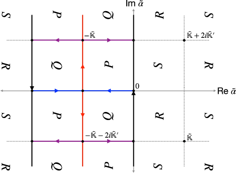
a. Periodicity of unit cells in $\tilde{\alpha}$ plane

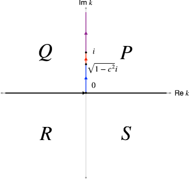
b. Image of $\tilde{\alpha}$ unit cells in $k$ plane

Figure 9: The Jacobi elliptic function relating $k$ and $\tilde{\alpha}$ in (4.66) is doubly periodic, satisfying $\text{sn}(\tilde{\alpha}+2\tilde{\mathbb{K}}+2i\tilde{\mathbb{K}}^{\prime}\rvert\tilde{m})=-\text{sn}\left(\tilde{\alpha}\rvert\tilde{m}\right)$, $\text{sn}\left(\tilde{\alpha}+2i\mathbb{K}^{\prime}\rvert\tilde{m}\right)=\text{sn}\left(\tilde{\alpha}\rvert\tilde{m}\right)$, as well as $\text{sn}\left(-\tilde{\alpha}\rvert\tilde{m}\right)=-\text{sn}\left(\tilde{\alpha}\rvert\tilde{m}\right)$. Thus, the unit cells in the $\tilde{\alpha}$ plane are arranged as shown in a. Each grouping of four neighboring tiles labelled ‘Q’, ‘P’, ‘R’ and ‘S’, which are the pre-images of the four quadrants in the $k$ plane as shown in b., is one unit cell. The intervals $(-\infty,0)$ and $(0,\infty)$ on the real axis and $(0,\sqrt{1-c^{2}}i)$, $(\sqrt{1-c^{2}}i,i)$ and $(i,+\infty i)$ in the $k$ plane are indicated in b. using black, blue, red and purple directed line segments, respectively. Their pre-images in the $\tilde{\alpha}$ plane are likewise indicated in a.

Next, we determine $g^{R/L}_{xx}$ as linear combinations of $\tilde{f}_{\pm}$. We cannot replicate (4.25) and (4.26) because $\Theta(\tilde{\sigma}_{\pm}|\tilde{m})=0$. Instead, the appropriate linear combinations are

$$g^{R}_{xx}(\tilde{\sigma};\tilde{\alpha}) \equiv\frac{1}{\Theta(\tilde{\sigma}|\tilde{m})}\left[\frac{H(\tilde{\sigma}+\tilde{\alpha}|\tilde{m})}{H(\tilde{\sigma}_{+}+\tilde{\alpha}|\tilde{m})}e^{(\tilde{\sigma}_{+}-\tilde{\sigma})Z(\tilde{\alpha}|\tilde{m})}-\frac{H(-\tilde{\sigma}+\tilde{\alpha}|\tilde{m})}{H(-\tilde{\sigma}_{+}+\tilde{\alpha}|\tilde{m})}e^{(\tilde{\sigma}-\tilde{\sigma}_{+})Z(\tilde{\alpha}|\tilde{m})}\right],$$ (4.67)

$$g^{L}_{xx}(\tilde{\sigma};\tilde{\alpha}) \equiv\frac{1}{\Theta(\tilde{\sigma}|\tilde{m})}\left[\frac{H(-\tilde{\sigma}+\tilde{\alpha}|\tilde{m})}{H(-\tilde{\sigma}_{-}+\tilde{\alpha}|\tilde{m})}e^{(\tilde{\sigma}-\tilde{\sigma}_{-})Z(\tilde{\alpha}|\tilde{m})}-\frac{H(\tilde{\sigma}+\tilde{\alpha}|\tilde{m})}{H(\tilde{\sigma}_{-}+\tilde{\alpha}|\tilde{m})}e^{(\tilde{\sigma}_{-}-\tilde{\sigma})Z(\tilde{\alpha}|\tilde{m})}\right].$$ (4.68)

Let us check that these indeed satisfy the boundary condition $g^{R}_{xx}(\tilde{\sigma},\tilde{\alpha})\to 0$ as $\tilde{\sigma}\to\tilde{\sigma}_{+}$ (and therefore also $g^{L}_{xx}(\tilde{\sigma},\tilde{\alpha})\to 0$ as $\tilde{\sigma}\to\tilde{\sigma}_{-}$). We note the behavior of $\Theta(\tilde{\sigma}|\tilde{m})$ near $\tilde{\sigma}=\tilde{\sigma}_{+}$,

$$\Theta(\tilde{\sigma}|\tilde{m})=\frac{\pi}{2\tilde{\mathbb{K}}}\theta_{4}^{\prime}\left(\frac{\pi\tilde{\tau}}{2},\tilde{q}\right)(\tilde{\sigma}-\tilde{\sigma}_{+})+O(\tilde{\sigma}-\tilde{\sigma}_{+})^{2},$$ (4.69)

where $\tilde{\tau}\equiv\frac{i\tilde{\mathbb{K}}^{\prime}}{\tilde{\mathbb{K}}}$ and $\tilde{q}\equiv e^{i\pi\tilde{\tau}}$. Furthermore, $\Theta$ is related to $H$ after a translation by $\pm i\tilde{\mathbb{K}}^{\prime}$:

$$H(\tilde{\sigma}\pm i\tilde{\mathbb{K}}^{\prime}|\tilde{m})=\pm i\text{exp}\left(\mp\frac{i\pi}{2\tilde{\mathbb{K}}}\left(\tilde{\sigma}\pm\frac{i\tilde{\mathbb{K}}^{\prime}}{2}\right)\right)\Theta(\tilde{\sigma}|\tilde{m}).$$ (4.70)

This allows us to express the $n$-fold derivatives of $H$ translated by half-periods (i.e., $H^{(n)}/H$ evaluated at $\tilde{\alpha}\pm i\tilde{\mathbb{K}}^{\prime}$) as sums of the lower derivatives of $\Theta$ (i.e., $\Theta^{(m)}/\Theta$ evaluated at $\tilde{\alpha}$ for $0\leq m\leq n$). Recalling also that $Z=\Theta^{\prime}/\Theta$, we ultimately find

$$g^{R}_{xx}(\tilde{\sigma};\tilde{\alpha}) =\frac{2\tilde{\mathbb{K}}}{3\pi}\frac{1}{\theta_{4}^{\prime}\left(\frac{\pi\tilde{\tau}}{2},\tilde{q}\right)}\left[\frac{\Theta^{\prime\prime\prime}(\tilde{\alpha}|\tilde{m})}{\Theta(\tilde{\alpha}|\tilde{m})}-\frac{3\Theta^{\prime\prime}(\tilde{\alpha}|\tilde{m})}{\Theta(\tilde{\alpha}|\tilde{m})}Z(\tilde{\alpha}|\tilde{m})+2Z^{3}(\tilde{\alpha}|\tilde{m})\right](\tilde{\sigma}-\tilde{\sigma}_{+})^{2}+O(\tilde{\sigma}-\tilde{\sigma}_{+})^{3}$$

$$=\frac{2\tilde{\mathbb{K}}}{3\pi}\frac{1}{\theta_{4}^{\prime}\left(\frac{\pi\tilde{\tau}}{2},\tilde{q}\right)}Z^{\prime\prime}(\tilde{\alpha}|\tilde{m})(\tilde{\sigma}-\tilde{\sigma}_{+})^{2}+O(\tilde{\sigma}-\tilde{\sigma}_{+})^{3}.$$ (4.71)

This reproduces the expected behavior in (4.12).

Thus, sending $g_{xx}^{R}(\tilde{\sigma};\tilde{\alpha})$ and $g_{xx}^{L}(\tilde{\sigma};\tilde{\alpha})$ to opposite boundaries yields

$$\lim_{\rho\to\infty}e^{2\rho}g_{xx}^{R}(\tilde{\sigma};\tilde{\alpha}) =\lim_{\rho\to-\infty}e^{-2\rho}g_{xx}^{L}(\tilde{\sigma};\tilde{\alpha})=-\frac{8\tilde{\mathbb{K}}}{3\pi}\frac{1-c^{2}}{\theta_{4}^{\prime}\left(\frac{\pi\tilde{\tau}}{2},\tilde{q}\right)}Z^{\prime\prime}(\tilde{\alpha}|\tilde{m}).$$ (4.72)

Furthermore, the normalization can be simplified to

$$a_{xx}(\tilde{\alpha}) =\frac{i}{\sqrt{1-c^{2}}}\left(2\frac{dg_{xx}^{R}(0;\tilde{\alpha})}{d\sigma}g_{xx}^{R}(0;\tilde{\alpha})\right)^{-1}$$ (4.73)

$$=-\frac{i\Theta(0|\tilde{m})^{2}e^{\frac{\pi\tilde{\mathbb{K}}^{\prime}}{2\tilde{\mathbb{K}}}}}{4\sqrt{1-c^{2}}}\left(\frac{H(\tilde{\alpha}|\tilde{m})^{2}}{\Theta(\tilde{\alpha}|\tilde{m})^{2}}\left(V(\tilde{\alpha}|\tilde{m})-Z(\tilde{\alpha}|\tilde{m})\right)\sinh\left(\frac{i\pi\tilde{\alpha}}{\tilde{\mathbb{K}}}+2i\tilde{\mathbb{K}}^{\prime}Z(\tilde{\alpha}|\tilde{m})\right)\right)^{-1},$$

where we used the fact that $a_{xx}(\tilde{\alpha})$ is independent of $\tilde{\sigma}$ to evaluate the Wronskian at $\tilde{\sigma}=0$.

Using $\frac{dk}{d\tilde{\alpha}}=-i\text{cn}\left(\tilde{\alpha}\rvert\tilde{m}\right)\text{dn}\left(\tilde{\alpha}\rvert\tilde{m}\right)$ (note (4.66) and (A.13)) and (A.36)-(A.38) to express various combinations of the theta functions in terms of the Jacobi elliptic functions, we may write the boundary limit of the bulk-to-bulk propagators as the following integral:

$$\lim_{\begin{subarray}{c}\rho\to\infty\\ \rho^{\prime}\to-\infty\end{subarray}}e^{2\rho-2\rho^{\prime}}G_{xx}(\rho,\tau;\rho^{\prime},\tau^{\prime}) =\frac{4\sqrt{1-c^{2}}}{9\pi g}\int_{-i\tilde{\mathbb{K}}^{\prime}}^{i\tilde{\mathbb{K}}^{\prime}}d\tilde{\alpha}\biggr{[}\text{exp}\left(\text{sn}\left(\tilde{\alpha}\rvert\tilde{m}\right)|\tau-\tau^{\prime}|\right)$$ (4.74)

$$\hskip 85.35826pt\times\frac{\text{sn}\left(\tilde{\alpha}\rvert\tilde{m}\right)\text{cn}^{2}\left(\tilde{\alpha}\rvert\tilde{m}\right)\text{dn}^{2}\left(\tilde{\alpha}\rvert\tilde{m}\right)}{\sinh\left(\tilde{F}(\tilde{\alpha})\right)}\biggr{]},$$

where

$$\tilde{F}(\tilde{\alpha}) \equiv\frac{i\pi\tilde{\alpha}}{\tilde{\mathbb{K}}}+2i\tilde{\mathbb{K}}^{\prime}Z(\tilde{\alpha}|\tilde{m}).$$ (4.75)

This is equivalent to (4.16) except with a different parametrization of the integration variable.

The next step is to close the contour in (4.74). The image of the contour in the $k$ plane can be closed in the upper-half plane at infinity. The lift to the $\tilde{\alpha}$ plane, shown in Figure 10 a., is not closed, but we can again use the periodicity of the map from $\tilde{\alpha}$ to $k$ to write (4.30) as one half of the integral over the closed contour shown in Figure 10 b.

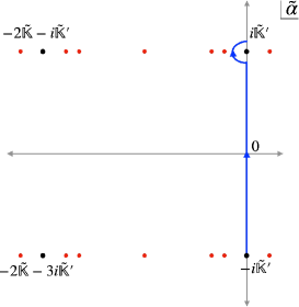
a.

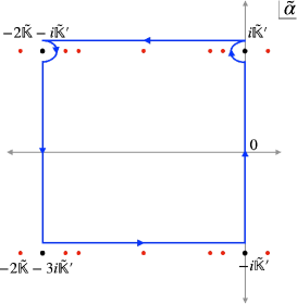
b.

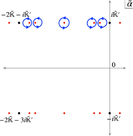
c.

Figure 10: Closing the integration contour in (4.74) and picking up the residues in the $\tilde{\alpha}$ plane. The integration contour along the real axis in the $k$ plane can be closed in the usual way at infinity in the upper half-plane. The lift of the closed contour to the $\alpha$ plane via the map in (4.66) is depicted in a. and is not closed. Using the periodic identification of the $\tilde{\alpha}$ plane as depicted in Figure 9, the contour in a. can be closed as in b. at the cost of doubling the integral. We can then pick up the residues at the poles on the interval $[-2\tilde{\mathbb{K}}-i\tilde{\mathbb{K}}^{\prime},i\tilde{\mathbb{K}}^{\prime}]$ parallel to the real axis, as depicted in c.

The poles of the integrand in (4.74) that lie inside the closed contour are the zeros of $\sinh(\tilde{F}(\tilde{\alpha}))$ that lie on the line segment between $i\tilde{\mathbb{K}}^{\prime}$ and $-2\tilde{\mathbb{K}}-i\tilde{\mathbb{K}}^{\prime}$ (see Figure 10 c), which we denote by $\tilde{\alpha}_{n}$, $n\in\mathbb{Z}$ and which satisfy

$$\tilde{F}(\tilde{\alpha}_{n})=(n-1)\pi i.$$ (4.76)

Here, we choose to define $\tilde{\alpha}_{n}$ by setting $\tilde{F}(\tilde{\alpha}_{n})$ equal to $(n-1)\pi i$ instead of equal to $n\pi i$ because it is then possible to relate $\tilde{\alpha}_{n}$ to $\alpha_{n}$ by a linear transformation independent of $n$. In particular, we checked numerically that the following identity relating $F(z)$ defined in (4.31) and $\tilde{F}(z)$ defined in (4.75) appears to hold:

$$F(i\mathbb{K}^{\prime}z)-\tilde{F}\left(-\tilde{\mathbb{K}}-(\tilde{\mathbb{K}}+i\tilde{\mathbb{K}}^{\prime})z\right)=\pi i,\hskip 28.45274pt\forall z\in\mathbb{C}.$$ (4.77)

Combined with (4.32) and (4.76), this identity implies that $\alpha_{n}$ and $\tilde{\alpha}_{n}$ are related by

$$\frac{\alpha_{n}}{i\mathbb{K}^{\prime}} =-\frac{\tilde{\alpha}_{n}+\tilde{\mathbb{K}}}{\tilde{\mathbb{K}}+i\tilde{\mathbb{K}}^{\prime}}.$$ (4.78)

Namely, the positions of the poles in (4.30) along the line segment between $-i\mathbb{K}^{\prime}$ and $i\mathbb{K}^{\prime}$ in the $\alpha$ plane are equal to the positions of the poles of (4.74) along the line segment between $-2\tilde{\mathbb{K}}-i\tilde{\mathbb{K}}^{\prime}$ and $i\tilde{\mathbb{K}}^{\prime}$ in the $\tilde{\alpha}$ plane, as measured in units in which the two line segments have unit lengths. This can be also been seen qualitatively by comparing Figure 10 with Figure 8.

As a consequence of (4.78), the quasi-energies defined in (4.37) are also equal to

$$E_{n}=-\text{sn}\left(\tilde{\alpha}_{n}|\tilde{m}\right).$$ (4.79)

Again using (4.33) to evaluate the residues of (4.74) at $\tilde{\alpha}_{n}$, we arrive at

$$\lim_{\begin{subarray}{c}\rho\to\infty\\ \rho^{\prime}\to-\infty\end{subarray}}e^{2\rho-2\rho^{\prime}}G_{xx}(\rho,\tau;\rho^{\prime},\tau^{\prime})$$ (4.80)

$$=\frac{4\sqrt{1-c^{2}}}{9\pi g}\sum_{n=-\infty}^{\infty}(-1)^{n+1}\frac{\text{sn}\left(\tilde{\alpha}_{n}\rvert\tilde{m}\right)\text{cn}^{2}\left(\tilde{\alpha}_{n}\rvert\tilde{m}\right)\text{dn}^{2}\left(\tilde{\alpha}_{n}\rvert\tilde{m}\right)\text{exp}\left(\text{sn}\left(\tilde{\alpha}_{n}\rvert\tilde{m}\right)|\tau-\tau^{\prime}|\right)}{\tilde{F}^{\prime}(\tilde{\alpha}_{n})}.$$

Using the identity in (A.37), we can write the derivative of $Z(\tilde{\alpha})|\tilde{m})$, and thus $\tilde{F}^{\prime}(\tilde{\alpha})$, in terms of the Jacobi elliptic functions. Using (A.3)-(A.6) to write $\tilde{\mathbb{K}}$, $\tilde{\mathbb{K}}^{\prime}$ and $\mathbb{E}(\frac{1}{1-c^{2}})$ in terms of $\mathbb{K}(c^{2})$ and $\mathbb{E}(c^{2})$, we find

$$\tilde{F}^{\prime}(z) =2i\sqrt{1-c^{2}}\mathbb{K}(c^{2})\left(\text{dn}\left(z|\tilde{m}\right)-1\right)+\frac{2i\mathbb{E}(c^{2})}{\sqrt{1-c^{2}}}.$$ (4.81)

Eq. (4.74) is the final integral representation and (4.80), supplemented with (4.76), is the final series representation for the boundary limit of $G_{xx}$ expressed in terms of the $\tilde{\alpha}$ variables. It is again more transparent to express both in terms of the original $k$ variables.

We first rewrite (4.74). $\tilde{F}$ can be written as a function of $k$ using $\tilde{F}(k)=\int_{0}^{k}dk^{\prime}\frac{d\tilde{\alpha}}{dk^{\prime}}\frac{d\tilde{F}}{d\tilde{\alpha}}$ and noting (4.81). Using (4.66) and (A.16)-(A.17), all of the elliptic functions can be expressed in terms of $k$. Ultimately, we find

$$W_{xx}(t_{1},t_{2}) =\frac{g}{\pi t_{12}^{4}}\frac{\chi^{4}}{(1-\chi)^{2}}\int_{-\infty}^{\infty}dk\frac{k\sqrt{1+k^{2}}\sqrt{1-c^{2}+k^{2}}\cos(k\log(\chi-1))}{\sinh\left(2\int_{0}^{k}d\ell\frac{\mathbb{K}(c^{2})\ell^{2}+\mathbb{E}(c^{2})}{\sqrt{1+\ell^{2}}\sqrt{1-c^{2}+\ell^{2}}}\right)}.$$ (4.82)

This is valid for $\chi>1$.

Finally, we use (A.16)-(A.17) and (4.79) to write all the elliptic functions in (4.80) in terms of $E_{n}$. The boundary-to-boundary propagator simplifies to

$$W_{xx}(t_{1},t_{2}) =\frac{12g}{\pi}\frac{1}{t_{12}^{4}}\frac{\chi^{4}}{(1-\chi)^{2}}\sum_{n\in\mathbb{Z}}\text{sgn}(1-\chi)^{n+1}f(E_{n})\frac{E_{n}^{2}-1}{6}e^{-E_{n}|\log|1-\chi||}.$$ (4.83)

Here $f(E)$ is the same function defined in (2.29). In the above expression, we have again replaced $(-1)^{n}$ in (4.80) by $\text{sgn}(1-\chi)^{n}$ in accordance with the discussion around (4.14)-(4.15), and the resulting series representation for $W_{xx}$ holds for both $\chi>1$ and $\chi<1$. Note that because $E_{0}=1$, the $n=0$ term in the sum is zero. Using $G_{4}(\chi)=\frac{\pi}{12g}t_{12}^{4}W_{xx}(t_{1},t_{2})$, this leads to (2.31).

Remarks about $G_{4}(\chi)$.

Now we make two remarks about the final result for $G_{4}(\chi)$. We can check that the four-point function reduces to the two-point function of the displacement operators when $c=0$. In this case the series representation of $W_{xx}(t_{1},t_{2})$ from (4.83) becomes

$$W_{xx}(t_{1},t_{2}) =\frac{2g}{\pi}\frac{1}{t_{12}^{4}}\frac{\chi^{4}}{(1-\chi)^{2}}\sum_{n=1}^{\infty}\text{sgn}(1-\chi)^{n+1}n(n+1)(n+2)e^{-(n+1)|\log|1-\chi||}.$$ (4.84)

Given that $\sum_{n=2}^{\infty}n(n^{2}-1)e^{-nx}=\frac{3}{8}\sinh^{-4}{\frac{x}{2}}$ and $\sum_{n=2}^{\infty}(-1)^{n}n(n^{2}-1)e^{-nx}=\frac{3}{8}\cosh^{-4}{\frac{x}{2}}$, we can explicitly sum the series for $\chi>1$ and $\chi<1$. In both cases, we arrive at the result

$$\braket{\mathbb{D}_{a}(t_{1})\mathbb{D}_{b}(t_{2})} =W_{xx}(t_{1},t_{2})\delta_{ab}=\frac{12g}{\pi}\frac{1}{t_{12}^{4}}\delta_{ab}.$$ (4.85)

This reproduces the leading behavior of (2.17).

Next, comparing (4.36) and (4.82) or (4.38) and (4.83), one sees that $G_{1}$ and $G_{4}$ satisfy:

$$G_{4}(\chi) =-\frac{\chi^{4}}{6}\left(3\frac{d}{d\chi}+(\chi-1)\frac{d^{2}}{d\chi^{2}}\right)\frac{G_{1}(\chi)}{\chi^{2}}.$$ (4.86)

This identity, in analogy with (2.26), should essentially be a Ward identity that relates the four-point functions in (2.13) and (2.14) that belong to the same superconformal multiplet.

5 Extracting OPE data from the four-point functions

In this section, we extract defect OPE data of operators with large charge from the four-point defect correlators in (2.13)-(2.14). The analysis in this case is particularly simple because the series representations of the defect correlators in (2.30)-(2.31) and (4.54)-(4.57) are already essentially in the form of conformal block expansions, and because the conformal blocks simplify when some of the operators have large dimensions. For a given four-point function, each term in the series corresponds to a different exchanged operator, the energies $E_{n}$ determine the anomalous dimensions, and the coefficients in the series determine the OPE coefficients. We also determine the small and large $\mathcal{J}$ behavior of the defect correlators and the OPE data.

5.1 Extracting OPE data

In a 1d CFT, the conformal block expansion of a four-point function in the $12\to 34$ channel is given by [69]

$$\braket{O_{1}(t_{1})O_{2}(t_{2})O_{3}(t_{3})O_{4}(t_{4})} =\frac{1}{t_{21}^{\Delta_{1}+\Delta_{2}}t_{43}^{\Delta_{3}+\Delta_{4}}}\left(\frac{t_{42}}{t_{41}}\right)^{\Delta_{1}-\Delta_{2}}\left(\frac{t_{41}}{t_{31}}\right)^{\Delta_{3}-\Delta_{4}}$$ (5.1)

$$\times\sum_{\Delta}p_{\Delta}\chi^{\Delta}{{}_{2}F_{1}}(\Delta+\Delta_{2}-\Delta_{1},\Delta+\Delta_{3}-\Delta_{4},2\Delta,\chi).$$

Here, we take the order of the operators to be $t_{1}<t_{2}<t_{3}<t_{4}$, in which case $0<\chi<1$. We will restrict our attention to four-point correlators in which $O_{1}^{\dagger}=O_{3}$ and $O_{2}^{\dagger}=O_{4}$ or $O_{1}^{\dagger}=O_{4}$ and $O_{2}^{\dagger}=O_{3}$, in which case we may choose a basis of primaries $O_{k}$ such that they satisfy the orthogonality condition $\braket{O_{k}O_{k^{\prime}}^{\dagger}}\propto\delta_{kk^{\prime}}$, and the OPEs in the $12\to 34$ channel take the form $O_{1}O_{2}\sim\sum_{k}\frac{\mathcal{C}_{O_{1}O_{2}O_{k}}}{\mathcal{N}_{O_{k}O_{k}^{\dagger}}}O_{k}$, $O_{3}O_{4}\sim\sum_{k}\frac{\mathcal{C}_{O_{3}O_{4}O_{k}}}{\mathcal{N}_{O_{k}O_{k}^{\dagger}}}O_{k}^{\dagger}$. The sum over $\Delta$ in (5.1) is then a sum over the primaries $O_{k}$ with $\Delta=\Delta_{k}$ and $p_{\Delta}=\mathcal{C}_{O_{1}O_{2}O_{k}}\mathcal{C}_{O_{3}O_{4}O_{k}^{\dagger}}/\mathcal{N}_{O_{k}O_{k}^{\dagger}}$.

We will study the conformal block expansions of the defect correlators in (2.13)-(2.14) in the “light-heavy”$\to$ “light-heavy” channels, in which case the exchanged operators appearing in the OPEs of both “light-heavy” pairs of the external operators have large charge and large conformal dimension. When multiple of the external and exchanged operators have large conformal dimensions, the conformal blocks simplify. In particular, two asymptotic expansions of the hypergeometric function that will be useful are

$${{}_{2}F_{1}}(\alpha,\beta,L+\gamma,\chi) =1+\frac{\alpha\beta}{L}\chi+O\left(\frac{1}{L^{2}}\right),$$ (5.2)

$${{}_{2}F_{1}}(L+\alpha,\beta,L+\gamma,\chi) =\frac{1}{(1-\chi)^{\beta}}\left(1+\frac{\beta(\alpha-\gamma)}{L}\frac{\chi}{1-\chi}+O\left(\frac{1}{L^{2}}\right)\right).$$ (5.3)

The first expansion follows from the series definition ${{}_{2}F_{1}}(a,b,c,\chi)\equiv 1+\frac{ab}{c}z+\frac{a(a+1)b(b+1)}{c(c+1)}z^{2}+\ldots$, and is relevant when $\Delta=\Delta_{1}+O(1)=\Delta_{4}+O(1)$ are large in (5.1). The second expansion can be found in, e.g., [70] and is relevant when $\Delta=\Delta_{2}+O(1)=\Delta_{4}+O(1)$ are large.

OPE data from $\braket{Z^{J}Z\bar{Z}\bar{Z}^{J}}$ and $\braket{ZZ^{J}\bar{Z}\bar{Z}^{J}}$.

Consider the conformal block expansion of $\braket{(\epsilon_{1}\cdot\Phi(t_{1}))^{J}\epsilon_{2}\cdot\Phi(t_{2})\epsilon_{3}\cdot\Phi(t_{3})(\epsilon_{4}\cdot\Phi(t_{4}))^{J}}$ in the $12\to 34$ channel. It decomposes into three different channels distinguished by the $SO(5)$ irreducible representations (irreps) of the operators that appear in the OPE of $(\epsilon_{1}\cdot\Phi)^{J}$ and $\epsilon_{2}\cdot\Phi$ (and likewise in the OPE of $\epsilon_{3}\cdot\Phi$ and $(\epsilon_{4}\cdot\Phi)^{J}$). In terms of Young tableaux, the decomposition of the tensor product of the rank $1$ and rank $J$ symmetric traceless representations into irreps is given by

$$\Yvcentermath 2\yng(1)\otimes\overbrace{\yng(5)}^{J}=\overbrace{\yng(6)}^{J+1}\oplus\overbrace{\yng(5,1)}^{J}\oplus\overbrace{\yng(4)}^{J-1},$$ (5.4)

The three $SO(5)$ channels can be disentangled and studied separately using, for instance, harmonic polynomials of $\xi$ and $\zeta$. However, for simplicity we choose instead to focus on the four-point correlator $\braket{Z^{J}(t_{1})Z(t_{2})\bar{Z}(t_{3})\bar{Z}^{J}(t_{4})}$, which has only one channel because the operators appearing in the OPE of $Z^{J}$ and $Z$ and in the OPE of $\bar{Z}$ and $\bar{Z}^{J}$ all transform in the rank $J+1$ representation. In principle, we do not lose anything with this restriction because the operators in the three channels are in the same superconformal multiplets, so their anomalous dimensions are the same and their OPE coefficients are related.

Relabelling $1\rightarrow 2\rightarrow 3\rightarrow 1$ in (2.20) and putting the resulting correlator in the form of (5.1) yields

$$\braket{Z^{J}(t_{1})Z(t_{2})\bar{Z}(t_{3})\bar{Z}^{J}(t_{4})} =\frac{4g\mathcal{N}_{Z^{J}\bar{Z}^{J}}/\pi}{t_{21}^{J+1}t_{43}^{J+1}}\left(\frac{t_{42}t_{31}}{t_{41}^{2}}\right)^{J-1}\frac{\chi^{J+1}}{(1-\chi)^{2}}G_{Z\bar{Z}}\left(\frac{\chi-1}{\chi}\right).$$ (5.6)

Here $\chi\equiv\frac{t_{12}t_{34}}{t_{13}t_{24}}$, as in previous sections. Applying (4.56), this may be explicitly written

$$\braket{Z^{J}(t_{1})Z(t_{2})\bar{Z}(t_{3})\bar{Z}^{J}(t_{4})} =\frac{4g\mathcal{N}_{Z^{J}\bar{Z}^{J}}/\pi}{t_{21}^{J+1}t_{43}^{J+1}}\left(\frac{t_{42}t_{31}}{t_{41}^{2}}\right)^{J-1}\biggr{[}\left(g\pi c^{2}\left(1+\frac{2\chi}{J}\right)+\frac{\pi}{2}\frac{1-c^{2}}{\mathbb{E}(c^{2})}\right)\chi^{J+1}$$

$$+\sum_{n=1}^{\infty}2f(E_{n})\frac{E_{n}+1}{E_{n}}\chi^{E_{n}+J+1}+O(1/g)\biggr{]}.$$ (5.7)

Here, we have combined the $n=0$ term in the sum in (4.56) with the term outside the sum (and recalled that $f(1)=\frac{g\pi c^{2}}{J}$) and also combined the $-n$ and $n$ terms.

Eq. (5.1) is in the form of a conformal block expansion. Let us denote the primaries appearing in the OPE of $Z^{J}$ and $Z$ by $[Z^{J}Z]_{n}$, the operators appearing in the OPE of $\bar{Z}$ and $\bar{Z}^{J}$ by $[\bar{Z}\bar{Z}^{J}]_{n}$, and their dimension by $\Delta_{n}$. Here $n=0,1,2\ldots$ is (for the moment) simply a label to distinguish the different operators, ordered by increasing conformal dimension. For instance, the lowest primaries are $[Z^{J}Z]_{0}\equiv Z^{J+1}$ and $[\bar{Z}\bar{Z}^{J}]_{0}\equiv\bar{Z}^{J+1}$. We take the primaries to satisfy $[Z^{J}Z]_{n}^{\dagger}=[\bar{Z}\bar{Z}^{J}]_{n}$ and $\braket{[ZZ^{J}]_{n}[\bar{Z}\bar{Z}^{J}]_{n^{\prime}}}\propto\delta_{nn^{\prime}}$.

We can now read off the OPE data of $[Z^{J}Z]_{n}$ and $[\bar{Z}\bar{Z}^{J}]_{n}$ by matching (5.1) to the general form of the conformal block expansion of $\braket{Z^{J}Z\bar{Z}\bar{Z}^{J}}$ given in (5.1). Identifying $\Delta_{1}=\Delta_{4}=J$, $\Delta_{2}=\Delta_{3}=1$ and $\Delta=\Delta_{n}$, and simplifying the conformal blocks using (5.2) with the identification $\alpha=\beta=\Delta_{n}+1-J$, $\gamma=2(\Delta_{n}-J)$ and $L=2J$, we arrive at

$$\braket{Z^{J}(t_{1})Z(t_{2})\bar{Z}(t_{3})\bar{Z}^{J}(t_{4})} =\frac{1}{t_{21}^{J+1}t_{43}^{J+1}}\left(\frac{t_{42}t_{31}}{t_{41}^{2}}\right)^{J-1}\sum_{n=0}^{\infty}\frac{\mathcal{C}_{Z^{J}Z[Z^{J}Z]_{n}}\mathcal{C}_{\bar{Z}\bar{Z}^{J}[\bar{Z}\bar{Z}^{J}]_{n}}}{\mathcal{N}_{[Z^{J}Z]_{n}[\bar{Z}\bar{Z}^{J}]_{n}}}\chi^{\Delta_{n}}$$ (5.8)

$$\hskip 113.81102pt\times\left(1+\frac{(\Delta_{n}+1-J)^{2}}{2J}\chi+O(1/g^{2})\right).$$

We can now compare (5.8) with (5.1) term-by-term, and read off the OPE data. To normalize the OPE coefficients by the norms of each of the operators, we note $\mathcal{N}_{Z\bar{Z}}=\frac{4g}{\pi}\left(1-\frac{3}{8\pi g}+\ldots\right)$, which follows from (2.17)-(2.18). Then, for the lowest operator, we find

$$\Delta_{0} =J+1, \frac{|\mathcal{C}_{Z^{J}ZZ^{J+1}}|^{2}}{\mathcal{N}_{Z\bar{Z}}\mathcal{N}_{Z^{J}\bar{Z}^{J}}\mathcal{N}_{Z^{J+1}\bar{Z}^{J+1}}} =g\pi c^{2}+\frac{\pi}{2}\frac{1-c^{2}}{\mathbb{E}(c^{2})}+\frac{3c^{2}}{8}+O(1/g).$$ (5.9)

This reproduces the OPE data that we used to fix the constants of integration of $G_{Z\bar{Z}}$ and $G_{\bar{Z}Z}$ in Section 4.2.2. Meanwhile, the higher terms in the conformal block expansion produce the new OPE data:

$$\Delta_{n} =J+1+E_{n}, \frac{|\mathcal{C}_{Z^{J}Z[Z^{J}Z]_{n}}|^{2}}{\mathcal{N}_{Z\bar{Z}}\mathcal{N}_{Z^{J}\bar{Z}^{J}}\mathcal{N}_{[ZZ^{J}]_{n}[\bar{Z}\bar{Z}^{J}]_{n}}} =2f(E_{n})\frac{E_{n}+1}{E_{n}},$$ (5.10)

where $n=1,2,3,\ldots$. In (5.9) and (5.10), we used $\mathcal{C}_{\bar{Z}\bar{Z}^{J}[\bar{Z}\bar{Z}^{J}]_{n}}=\mathcal{c}^{*}_{Z^{J}Z[Z^{J}Z]_{n}}$, which follows from reflection positivity of the dCFT. Because the simplified form of the conformal block in (5.2) is valid when $\alpha,\beta,\gamma\ll L$, the OPE data in (5.10) is reliable as long as $\Delta_{n}-J\ll J\sim\sqrt{\lambda}$. In the strict large charge limit, where the charge $J$ and string tension $\frac{\sqrt{\lambda}}{2\pi}$ are taken to infinity, (5.10) gives the OPE data of an infinite tower of non-protected operators.

As a non-trivial check, we can also extract OPE data from $\braket{Z(t_{1})Z^{J}(t_{2})\bar{Z}(t_{3})\bar{Z}^{J}(t_{4})}$, in which we switch the relative order of $Z$ and $Z^{J}$. Relabelling $1\leftrightarrow 2$ in (2.20), writing the correlator explicitly using (4.56), and putting it in the form of (5.1), we get

$$\braket{Z(t_{1})Z^{J}(t_{2})\bar{Z}(t_{3})\bar{Z}^{J}(t_{4})} =\frac{4g\mathcal{N}_{Z^{J}\bar{Z}^{J}}/\pi}{t_{21}^{J+1}t_{43}^{J+1}}\left(\frac{t_{42}}{t_{31}}\right)^{1-J}\chi^{J+1}G_{Z\bar{Z}}(\chi^{-1}),$$ (5.11)

$$=\frac{4g\mathcal{N}_{Z^{J}\bar{Z}^{J}}/\pi}{t_{21}^{J+1}t_{43}^{J+1}}\biggr{[}\left(g\pi c^{2}\left(1-\frac{2}{J}\frac{\chi}{1-\chi}\right)+\frac{\pi}{2}\frac{1-c^{2}}{\mathbb{E}(c^{2})}\right)\frac{\chi^{J+1}}{(1-\chi)^{2}}$$

$$+\sum_{n=1}^{\infty}(-1)^{n+1}\frac{2f(E_{n})(E_{n}+1)}{E_{n}}\frac{\chi^{J+1+E_{n}}}{(1-\chi)^{E_{n}+2}}+O(1/g)\biggr{]}.$$ (5.12)

We want to match (5.12) to the general form of the conformal block expansion in (5.1). We again denote the primaries appearing in the OPE of $Z$ and $Z^{J}$ by $[ZZ^{J}]_{n}\equiv[Z^{J}Z]_{n}$ and in the OPE of $\bar{Z}$ and $\bar{Z}^{J}$ by $[\bar{Z}\bar{Z}^{J}]_{n}$. Then, identifying $\Delta_{1}=\Delta_{3}=1$, $\Delta_{2}=\Delta_{4}=J$ and $\Delta=\Delta_{n}$ in (5.1), which allows us to simplify the conformal blocks using (5.3) if we set $L=2J$, $\alpha=\Delta_{n}-1-J$, $\beta=\Delta_{n}+1-J$, $\gamma=2(\Delta_{n}-J)$, we may write

$$\braket{Z(t_{1})Z^{J}(t_{2})\bar{Z}(t_{3})\bar{Z}^{J}(t_{4})}=\frac{1}{t_{21}^{J+1}t_{43}^{J+1}}\left(\frac{t_{42}}{t_{31}}\right)^{1-J}\sum_{n=0}^{\infty}\frac{\mathcal{C}_{ZZ^{J}[ZZ^{J}]_{n}}\mathcal{C}_{\bar{Z}\bar{Z}^{J}[\bar{Z}\bar{Z}^{J}]_{n}}}{\mathcal{N}_{[ZZ^{J}]_{n}[\bar{Z}\bar{Z}^{J}]_{n}}}\frac{\chi^{\Delta_{n}}}{(1-\chi)^{\Delta_{n}+1-J}}$$

$$\ \hskip 170.71652pt\times\left(1-\frac{(\Delta_{n}+1-J)^{2}}{2J}\frac{\chi}{1-\chi}+O(1/g^{2})\right).$$ (5.13)

We can now compare (5.1) with (5.12) term-by-term. For the lowest operator, we find

$$\Delta_{0} =J+1, \frac{\mathcal{C}_{ZZ^{J}Z^{J+1}}\mathcal{C}_{\bar{Z}\bar{Z}^{J}\bar{Z}^{J+1}}}{\mathcal{N}_{Z\bar{Z}}\mathcal{N}_{Z^{J}\bar{Z}^{J}}\mathcal{N}_{Z^{J+1}\bar{Z}^{J+1}}} =g\pi c^{2}+\frac{\pi}{2}\frac{1-c^{2}}{\mathbb{E}(c^{2})}+\frac{3c^{2}}{8}+O(1/g).$$ (5.14)

For the higher terms in the conformal block expansion, we find

$$\Delta_{n} =J+1+E_{n}, \frac{\mathcal{C}_{ZZ^{J}[ZZ^{J}]_{n}}\mathcal{C}_{\bar{Z}\bar{Z}^{J}[\bar{Z}\bar{Z}^{J}]_{n}}}{\mathcal{N}_{Z\bar{Z}}\mathcal{N}_{Z^{J}\bar{Z}^{J}}\mathcal{N}_{[ZZ^{J}]_{n}[\bar{Z}\bar{Z}^{J}]_{n}}} =(-1)^{n+1}\frac{2f(E_{n})(E_{n}+1)}{E_{n}},$$ (5.15)

for $n=1,2,3,\ldots$. Eqs. (5.14)-(5.15) match (5.9)-(5.10) as long as $\mathcal{C}_{ZZ^{J}[Z^{J}Z]_{0}}=\mathcal{C}_{Z^{J}Z[ZZ^{J}]_{0}}$ and $\mathcal{C}_{ZZ^{J}[Z^{J}Z]_{n}}=(-1)^{n+1}\mathcal{C}_{Z^{J}Z[ZZ^{J}]_{n}}$, for $n=1,2,\ldots$. This is a consequence of parity, assuming $[Z^{J}Z]_{n}$ is odd for $n=2,4,\ldots$ and even otherwise. These parities of the exchanged operators are consistent with the observation that in the generalized free field limit (i.e., $g\to\infty$, which can be probed via the $J/g\to 0$ limit of the large charge results) composite primaries can be constructed out of $J+1$ copies of $Z$ and $0,2,3,4,\ldots$ derivatives (thus, the operators $[ZZ^{J}]_{n}$ for $n>0$ contain $n+1$ derivatives), but no primary can be constructed using a single derivative because $Z^{J}\partial Z\sim\partial Z^{J+1}$ is a descendent. See Appendix D.2 for more details.

The OPE data derived in this section come with a caveat. When extracting OPE data from the conformal block expansion of a four-point function, if one does not make sure to disentangle the contributions of operators with the same quantum numbers, the extracted OPE data will in general be averages over the degenerate operators. Therefore, on general grounds we would expect the OPE data in (5.10) and (5.15) to be “mixing-averaged.” On the other hand, since we can precisely match the series representations of the four-point functions to the conformal block expansion, it is possible that the operator mixing is not relevant in the large charge limit. It would be good to understand this issue better.

5.2 Defect correlators and OPE data at small and large $\mathcal{J}$

In this section we examine the small $\mathcal{J}$ and large $\mathcal{J}$ behavior of the defect correlators derived in Section 4 and of the OPE data derived in Section 5.1.

Small $\mathcal{J}$.

We first consider the defect correlators in the regime $1\ll J\ll g$, in which case $\mathcal{J}$ is small. The series in (2.30)-(2.31) and (4.54)-(4.57) allow us to determine with minimal effort the small $c^{2}$ expansions of the defect correlators, which can be converted to small $\mathcal{J}$ expansions using the Taylor series relating $\mathcal{J}$ and $c^{2}$ in this regime:

$$\mathcal{J} =\pi c^{2}+\frac{3\pi c^{4}}{8}+\frac{15\pi c^{6}}{64}+O(c^{8}), c^{2} =\frac{1}{\pi}\mathcal{J}-\frac{3}{8\pi^{2}}\mathcal{J}^{2}+\frac{3}{64\pi^{3}}\mathcal{J}^{3}+O\left(\mathcal{J}^{4}\right).$$ (5.16)

We begin by determining the behavior of $E_{n}$ when $c^{2}$ is small. Qualitatively, the $E_{n}$ will be spaced approximately uniformly with unit separation, and deviations will be small in $c^{2}$ as long as $|n|$ is not too large. We can make this precise by determining the expansion of $E_{n}$ as a series in $c^{2}$. Recall that $E_{0}=1$ exactly for all $c$. Meanwhile, the divergence of $\rho(E)$ in (2.28) at $E=1$ makes determining the series expansion of $E_{n}$ for $n\neq 0$ directly from (2.27) a bit subtle, because naively expanding $\rho(E)$ in small $c^{2}$ and then integrating from $1$ to $E_{n}$ order by order yields divergent integrals at each order. Therefore, we rewrite (2.27) in terms of an integral that runs from $E_{n}$ to infinity, instead of from $1$ to $E_{n}$, in order to avoid the problematic point $E=1$:

$$E_{n}-\int_{E_{n}}^{\infty}\left[\frac{E^{2}-\mathbb{E}(c^{2})/\mathbb{K}(c^{2})}{\sqrt{E^{2}-1}\sqrt{E^{2}+c^{2}-1}}-1\right]dE =\frac{\pi}{2\mathbb{K}(c^{2})}(1+|n|).$$ (5.18)

For fixed $E_{n}>1$, it is now safe to expand the integrand in small $c^{2}$ and then integrate order by order, which yields rational functions of $E_{n}$ at each order. Writing $E_{n}=1+|n|+E_{n}^{(1)}c^{2}+E_{n}^{(2)}c^{4}+E_{n}^{(3)}c^{6}+\ldots$, we can then determine the $E_{n}^{(i)}$ by matching powers of $c^{2}$ on both sides of (5.18). We ultimately find

$$E_{0} =1,$$ (5.19)

$$E_{n} =1+|n|-\frac{|n|+1}{4}c^{2}-\frac{(|n|+1)(5n^{2}+10|n|-4)}{64|n|(|n|+2)}c^{4}$$

$$\hskip 50.07669pt-\frac{(|n|+1)(11n^{2}+22|n|-12)}{256|n|(|n|+2)}c^{6}+\ldots.\hskip 85.35826pt(n\neq 0)$$ (5.20)

The above series expansion is reliable as long as $|n|\ll 1/c^{2}$.

Given the series expansion of $E_{n}$, it is straightforward to expand the summands in (2.30)-(2.31) and (4.54)-(4.57) in small $c^{2}$ and evaluate the sums order by order. For instance, the first two terms for the small $c^{2}$ expansion of the defect correlators are given explicitly by:

$$G_{1}(\chi) =1+\frac{c^{2}}{4}\left[\frac{(-2+\chi+\chi^{3})\log|1-\chi|}{\chi}-\frac{(2+\chi(\chi-2))(1-\chi+\chi^{2}\log|\chi|)}{(\chi-1)^{2}}\right]+O(c^{4}),$$ (5.21)

$$G_{2}(\chi) =\frac{g\pi c^{2}\chi^{2}}{(1-\chi)^{2}}+\frac{c^{2}}{4(\chi-1)^{3}}\biggr{[}(1-\chi)(1+\chi^{2})(\chi+(1-\chi)^{2})\log|1-\chi|$$ (5.22)

$$\hskip 42.67912pt+\chi^{3}(4-3\chi+\chi^{2})\log|\chi|\biggr{]}+O(c^{4}),$$

$$G_{3}(\chi) =g\pi c^{2}\chi^{2}+\frac{c^{2}}{4(1-\chi)^{2}}\biggr{[}\chi(1-\chi)(1-2\chi+\chi^{2})$$ (5.23)

$$\hskip 42.67912pt+(1-\chi)^{3}(1+\chi+2\chi^{2})\log|1-\chi|+\chi^{3}(4-5\chi+2\chi^{2})\log|\chi|\biggr{]}+O(c^{4}),$$

$$G_{4}(\chi) =1+c^{2}\left[\left(\frac{1}{2}-\frac{1}{\chi}\right)\log|1-\chi|-1\right]+O(c^{4}).$$ (5.24)

Using the same procedure, it is relatively easy to determine the first few higher order corrections to the defect correlators. Instead of providing explicit expressions, we summarize the type of functions that appear in the expansion up to order $c^{10}$, which may potentially be useful if one were to try to identify a suitable ansatz to “‘bootstrap” these or related correlators. At order $c^{2n}$, the $G_{i}(\chi)$ are sums of products of the polylogarithm function $\text{Li}_{s}$ such that the sum of the polylogarithmic orders of any of the products of polylogarithmic functions is less than or equal to $n$. For instance, for the first few terms in the small $c^{2}$ expansion, the combinations of polylogarithms of “highest order” are logarithms at order $c^{2}$, products of pairs of logarithms at order $c^{4}$, and terms schematically of the form $\text{Li}_{3}$, $\log\cdot\text{Li}_{2}$ and $\log^{3}$ appearing at order $c^{6}$. However, not every product of polylogarithms “allowed” by the above rule appears at a given order. For instance, there is no $\text{Li}_{2}$ term at $c^{4}$, and no $\text{Li}_{4}$ or $\text{Li}_{2}^{2}$ terms at $c^{8}$.

We can also determine the small $\mathcal{J}$ expansion of the OPE data of the operators exchanged in the light-heavy channel of $\braket{ZZ^{J}\bar{Z}\bar{Z}^{J}}$, which were determined for finite $\mathcal{J}$ in (5.14)-(5.15). The first few terms in the expansions of the conformal dimensions are:

$$\Delta_{0} =J+1, \Delta_{n} =J+\left(2+n-\frac{n+1}{4\pi}\mathcal{J}+O(\mathcal{J}^{2})\right)+O(1/g),$$ (5.25)

The first few terms in the expansions of the OPE coefficients are:

$$\frac{\mathcal{C}_{ZZ^{J}Z^{J+1}}\mathcal{C}_{\bar{Z}\bar{Z}^{J}\bar{Z}^{J+1}}}{\mathcal{N}_{Z\bar{Z}}\mathcal{N}_{Z^{J}\bar{Z}^{J}}\mathcal{N}_{Z^{J+1}\bar{Z}^{J+1}}} =g\left(\mathcal{J}-\frac{3}{8\pi}\mathcal{J}^{2}+O(\mathcal{J}^{3})\right)+\left(1-\frac{3\mathcal{J}}{8\pi}+O(\mathcal{J}^{2})\right)+O(1/g^{2})$$ (5.26)

$$\frac{\mathcal{C}_{ZZ^{J}[ZZ^{J}]_{n}}\mathcal{C}_{\bar{Z}\bar{Z}^{J}[\bar{Z}\bar{Z}^{J}]_{n}}}{\mathcal{N}_{Z\bar{Z}}\mathcal{N}_{Z^{J}\bar{Z}^{J}}\mathcal{N}_{[ZZ^{J}]_{n}[\bar{Z}\bar{Z}^{J}]_{n}}} =(-1)^{n+1}\left(n+2-\frac{(n+2)(2n-1)}{4\pi n}\mathcal{J}+O(\mathcal{J}^{2})\right)+O(1/g).$$ (5.27)

In (5.25) and (5.27), $n=1,2,3,\ldots$. Note that $\Delta_{1}=\Delta_{0}+2$ when $\mathcal{J}=0$, which again corresponds to the fact that there is no composite primary in the generalized free field limit constructed out of $J+1$ copies of $Z$ and a single derivative (i.e., the $n=1$ operator corresponds in the free limit to a primary built out of $Z$ and $Z^{J}$ and two derivatives).

Finally, we note that an alternative approach to probing the defect correlators in the $1\ll J\ll g$ regime is to first take $J$ finite and expand in $1/g$ (which is the usual strong coupling expansion of the Wilson line dCFT that can be studied using Witten diagrams on the AdS₂ dual string), and only then take $J$ to be large. We show in Appendix D that the results of the finite charge analysis match the large charge results in (5.21)-(5.27).

Large $\mathcal{J}$.

The other limiting case of the defect correlators that is natural to consider is the regime $1\ll g\ll J$, in which case $\mathcal{J}$ is large. The series in (2.30)-(2.31) and (4.54)-(4.57) allow us to determine the leading behaviors of the defect correlators as $\mathcal{J}\to\infty$ or, equivalently, $c^{2}\to 1$. We note for convenience the asymptotic expansions relating $\mathcal{J}$ and $c^{2}$ in this regime:

$$\mathcal{J} =-2\log(1-c^{2})+4(2\log{2}-1)+O((1-c^{2})\log(1-c^{2})),$$ (5.28)

$$c^{2} =1-\frac{16}{e^{2}}e^{-\frac{\mathcal{J}}{2}}+O(\mathcal{J}e^{-\mathcal{J}}).$$ (5.29)

We first determine the behavior of the energies, $E_{n}$, when $\mathcal{J}\to\infty$. Because $\mathbb{K}(c^{2})\to\infty$ as $c\to 1$, it follows from (2.28) that, in this limit, the $E_{n}$ condense into a continuum with a smooth distribution. The density of the $E_{n}$, normalized by the large charge, is asymptotically

$$\frac{\rho(E)}{\mathcal{J}} \sim\frac{1}{2\pi}\frac{E}{\sqrt{E^{2}-1}}+\frac{2}{\pi}\frac{\sqrt{E^{2}-1}}{E}\frac{1}{\mathcal{J}}+O(e^{-\frac{\mathcal{J}}{2}}), \text{as }\mathcal{J}\to\infty.$$ (5.30)

The fine-grained behavior of the $E_{n}$ when $\mathcal{J}\to\infty$ can also be determined from the above density. Neglecting the exponentially suppressed term in $\rho(E)$, which is valid as long as $|n|\ll e^{\mathcal{J}}$, we can evaluate the integral in (2.27) and the quantization condition becomes

$$\frac{\mathcal{J}+4}{2\pi}\sqrt{E_{n}^{2}-1}-\frac{2}{\pi}\arctan\left(\sqrt{E_{n}^{2}-1}\right)+O(e^{-\mathcal{J}/2}) =|n|.$$ (5.31)

This lets us determine $E_{n}$ in various regimes. When $|n|\ll\mathcal{J}$ (i.e., $E\approx 1$), the $E_{n}$ may be expanded in $1/\mathcal{J}$:

$$E_{n} =1+\frac{2\pi^{2}n^{2}}{\mathcal{J}^{2}}-\frac{2\pi^{4}n^{4}}{\mathcal{J}^{4}}-\frac{64\pi^{4}n^{4}}{3\mathcal{J}^{5}}+\frac{4\pi^{6}n^{6}}{\mathcal{J}^{6}}+O(1/\mathcal{J}^{7}).$$ (5.32)

When $\mathcal{J}\ll|n|\ll e^{\mathcal{J}}$ (i.e., $E_{n}\gg 1$), the $E_{n}$ may be expanded in $1/|n|$:

$$E_{n} =\frac{2\pi|n|}{4+\mathcal{J}}+\frac{2\pi}{4+\mathcal{J}}+\frac{\mathcal{J}-4}{4\pi|n|}+\frac{4-\mathcal{J}}{4\pi n^{2}}+O(1/|n|^{3}).$$ (5.33)

Finally, when $|n|\sim\mathcal{J}$ (i.e., $E_{n}\sim 1$), we may write $n=\eta\mathcal{J}$ and expand in $1/\mathcal{J}$:

$$E_{n} =\sqrt{1+4\pi^{2}\eta^{2}}+\frac{8\pi\eta(-2\pi\eta+\arctan(2\pi\eta))}{\sqrt{1+4\pi^{2}\eta^{2}}}\frac{1}{\mathcal{J}}$$ (5.34)

$$\hskip 56.9055pt+\frac{8(2\pi\eta-\arctan(2\pi\eta))(2\pi\eta-\arctan(2\pi\eta)+16\pi^{3}\eta^{3})}{(1+4\pi^{2}\eta^{2})^{\frac{3}{2}}}\frac{1}{\mathcal{J}^{2}}+O(1/\mathcal{J}^{3}).$$

The leading term in (5.34) precisely matches the expression for the energy of fluctuations about the $c^{2}=1$ string in the BMN limit, which was derived in [8]. In particular, [8] found that the fluctuations have energies $\omega_{p}=\sqrt{1+p^{2}}$ and argued that the boundary conditions fix the momenta to be $p_{n}=\frac{n\sqrt{\lambda}}{2J}$ with $n\in\mathbb{Z}$. We note that in (5.34), $2\pi\eta=\frac{2\pi ng}{J}=\frac{n\sqrt{\lambda}}{2J}.$

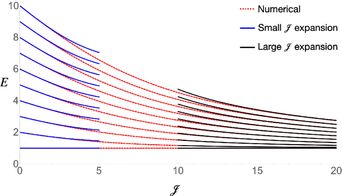
Figure 11: $E_{n}$ is plotted for $n=0,1,2,\ldots,9$ and $\mathcal{J}\in[0,20]$. The red dashed curves depict the numerical values of $E_{n}$ computed using (2.27). The blue curves depict the small $c^{2}$ expansion given in (5.20). The black curves depict the large $\mathcal{J}$ expansion given in (5.34).

We can also study the four-point functions in the limit $\mathcal{J}\to\infty$. The condensation of the $E_{n}$ into a continuum makes it possible to convert the series representations of the $G_{i}(\chi)$ in (2.30)-(2.31) and (4.54)-(4.57) into simple integrals. In particular, we first note that $f(E)$ in (2.29) asymptotically approaches

$$f(E) \to\frac{\pi E}{\mathcal{J}}-\frac{4\pi}{\mathcal{J}^{2}}\frac{E^{2}-1}{E}+O(e^{-\frac{\mathcal{J}}{2}}), \text{as }\mathcal{J}\to\infty,$$ (5.35)

and therefore $\rho(E)f(E)\to\frac{E^{2}}{2\sqrt{E^{2}-1}}$ is finite in the limit $\mathcal{J}\to\infty$. This is useful because, given a smooth function $g(E)$, the sum $\sum_{n\in\mathbb{Z}}f(E_{n})g(E_{n})$ approaches the integral $\int dE\frac{E^{2}}{\sqrt{E^{2}-1}}g(E)$ as $\mathcal{J}\to\infty$. When $\chi<1$ and the terms in the series are all positive, we can apply this to the series in (2.30) and (2.31) and find

$$G_{1}(\chi) \to\frac{\chi^{2}}{1-\chi}\int_{1}^{\infty}dE\frac{E^{2}}{\sqrt{E^{2}-1}}e^{-E|\log(1-\chi)|}$$

$$=\frac{\chi^{2}}{1-\chi}K_{0}^{\prime\prime}(|\log(1-\chi)|)$$ (5.36)

$$G_{4}(\chi) \to\frac{\chi^{4}}{(1-\chi)^{2}}\int_{1}^{\infty}dE\frac{E^{2}}{\sqrt{E^{2}-1}}\frac{E^{2}-1}{6}e^{-E|\log(1-\chi)|}$$

$$=\frac{1}{6}\frac{\chi^{4}}{(1-\chi)^{2}}\biggr{[}K_{0}^{\prime\prime\prime\prime}(|\log(1-\chi)|)-K_{0}^{\prime\prime}(|\log(1-\chi)|)\biggr{]}.$$ (5.37)

Similarly, from the piecewise series representations of $G_{Z\bar{Z}}$ and $G_{\bar{Z}Z}$ in (4.54)-(4.57), we also find

$$G_{Z\bar{Z}}(\chi) \to g\pi\frac{\chi^{2}}{(1-\chi)^{2}}+\frac{\chi^{2}}{1-\chi}\int_{1}^{\infty}\frac{E^{2}}{\sqrt{E^{2}-1}}\frac{E\pm 1}{E}e^{-(E\pm 1)|\log(1-\chi)|}$$

$$=g\pi\frac{\chi^{2}}{(1-\chi)^{2}}+\frac{\chi^{2}}{(1-\chi)^{2}}\biggr{[}K_{0}^{\prime\prime}(|\log(1-\chi)|)\mp K_{0}^{\prime}(|\log(1-\chi)|)\biggr{]},$$ (5.38)

$$G_{\bar{Z}Z}(\chi) \to g\pi\chi^{2}+\frac{\chi^{2}}{1-\chi}\int_{1}^{\infty}\frac{E^{2}}{\sqrt{E^{2}-1}}\frac{E\mp 1}{E}e^{-(E\mp 1)|\log(1-\chi)|}$$

$$=g\pi\chi^{2}+\chi^{2}\biggr{[}K_{0}^{\prime\prime}(|\log(1-\chi)|)\pm K_{0}^{\prime}(|\log(1-\chi)|)\biggr{]},$$ (5.39)

where the upper (lower) sign is for $\chi<0$ ($0<\chi<1$). In these expressions, $K_{0}(z)$ is the modified Bessel function of the second kind.

By contrast, when $\chi>1$, the series become alternating and vanish in the continuum limit. Thus, we find the following simplified asymptotic behavior as $\mathcal{J}\to\infty$:

$$G_{1}(\chi),G_{4}(\chi) \to 0, G_{Z\bar{Z}}(\chi) \to g\pi\frac{\chi^{2}}{(1-\chi)^{2}}, G_{\bar{Z}Z}(\chi) \to g\pi\chi^{2}.$$ (5.41)

These can also be seen from the fact that the $\sinh$ term in the integrands in (4.36),(4.58)-(4.59) and (4.84) diverges as $c^{2}\to 1$.

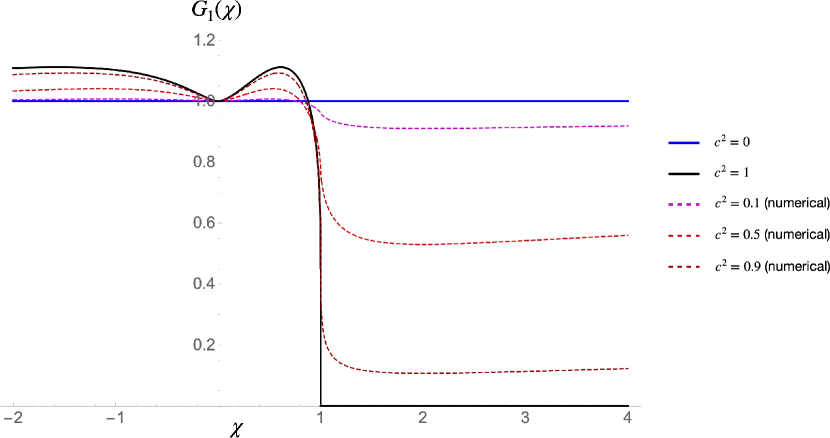
Figure 12: $G_{1}(\chi)$ is plotted as a function of $\chi$ for representative values of $c^{2}$. The solid blue curve depicts $G_{1}(\chi)=1$, corresponding to the edge case $c^{2}=0$ (i.e., $\mathcal{J}=0$). The solid black curve depicts $G_{1}(\chi)$ for the edge case $c^{2}=1$ (i.e., $\mathcal{J}=\infty$), given by (5.36) and (5.41). The dashed curves depict $G_{1}(\chi)$ for $c^{2}=0.1,0.5,0.9$, evaluated numerically using the series representation in (2.30) for $\chi<1$ and using the integral representation in (4.36) for $\chi>1$. The numerical results on a small interval around $\chi=0$ are excluded due to slow convergence of the series. One can also plot $G_{1}(\chi)$ for $\chi>1$ using the series in (4.36); the resulting curve matches the curve from the integral representation, but convergence is slow near $\chi=2$.

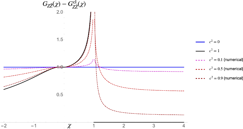
Figure 13: The fluctuation component of $G_{Z\bar{Z}}(\chi)$ is plotted as a function of $\chi$ for representative values of $c^{2}$.

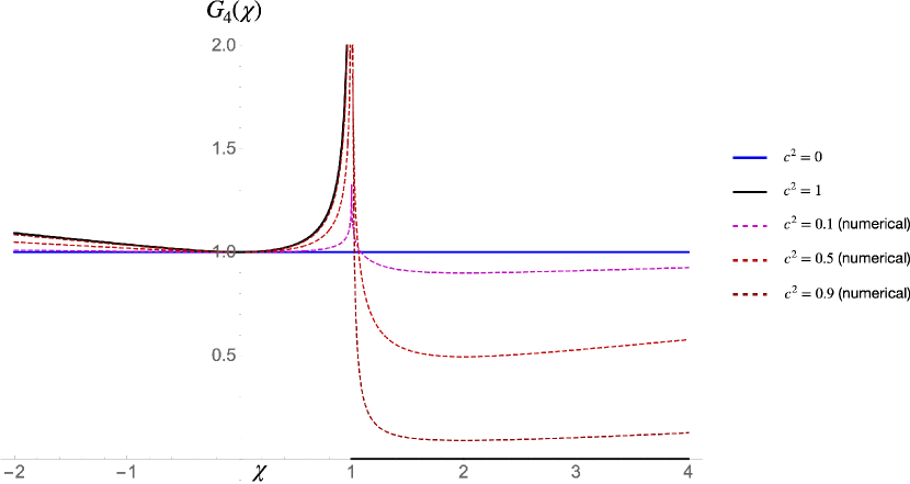
Figure 14: $G_{4}(\chi)$ is plotted as a function of $\chi$ for representative values of $c^{2}$.

Finally, we note the large $\mathcal{J}$ expansion of the OPE data of the operators exchanged in the light-heavy channel of $\braket{ZZ^{J}\bar{Z}\bar{Z}^{J}}$, which were determined for finite $\mathcal{J}$ in (5.14)-(5.15). The leading terms in the expansions of the conformal dimensions are:

$$\Delta_{0} =J+1, \Delta_{n} =J+\left(1+\sqrt{1+4\pi^{2}\eta^{2}}+O(1/\mathcal{J})\right)+O(1/g),$$ (5.42)

The leading terms in the expansions of the OPE coefficients are:

$$\frac{\mathcal{C}_{ZZ^{J}Z^{J+1}}\mathcal{C}_{\bar{Z}\bar{Z}^{J}\bar{Z}^{J+1}}}{\mathcal{N}_{Z\bar{Z}}\mathcal{N}_{Z^{J}\bar{Z}^{J}}\mathcal{N}_{Z^{J+1}\bar{Z}^{J+1}}} =g\pi\left(1+O(e^{-\frac{\mathcal{J}}{2}})\right)+\biggr{(}\frac{3}{8}+O(e^{-\frac{\mathcal{J}}{2}})\biggr{)}+O(1/g)$$ (5.43)

$$\frac{\mathcal{C}_{ZZ^{J}[ZZ^{J}]_{n}}\mathcal{C}_{\bar{Z}\bar{Z}^{J}[\bar{Z}\bar{Z}^{J}]_{n}}}{\mathcal{N}_{Z\bar{Z}}\mathcal{N}_{Z^{J}\bar{Z}^{J}}\mathcal{N}_{[ZZ^{J}]_{n}[\bar{Z}\bar{Z}^{J}]_{n}}} =(-1)^{n+1}\left(\frac{2\pi}{\mathcal{J}}\left(1+\sqrt{1+4\pi^{2}\eta^{2}}\right)+O(1/\mathcal{J}^{2})\right)+O(1/g).$$ (5.44)

Eq. (5.42) and (5.44) are valid for $\eta\equiv n/\mathcal{J}\sim 1$.

Having determined exact expressions for the energies and the four-point functions (which can be evaluated numerically with relative ease), as well as simplified analytic results when $\mathcal{J}$ is small or large, we close this section by summarizing our findings in a series of figures. Figure 11 illustrates the dependence of the first few energies $E_{n}$ on $\mathcal{J}$. We include the exact results evaluated numerically via the quantization condition (2.27), and compare them with the small $c^{2}$ expansion in (5.20) and the large $\mathcal{J}$ expansion in (5.34). Furthermore, Figures 12-14 depict $G_{1}(\chi)$, $G_{Z\bar{Z}}(\chi)$, and $G_{4}(\chi)$ for representative values of $c^{2}$, combining the simple analytic results for $c^{2}=0$ given in (5.21)-(5.24) and for $c^{2}=1$ given in (5.36)-(5.41) with the numerical implementation of the series representations given in (2.30)-(2.31) and (4.54)-(4.57).

6 Connections to integrability

We now show that the results obtained in Section 4 can be interpreted naturally in terms of the (semi-)classical integrability of the string sigma model.

6.1 Classical integrability, spectral curve, and quasi-momentum

Let us first give a lightening review of the classical integrability of the closed string. For more details, we refer the readers to the original papers [51, 52, 53] or a review [72].

Spectral curve, quasi-momenta.

The Green-Schwarz string sigma model on AdS${}_{5}\times S^{5}$ is known to be classically integrable. The simplest way to see it is to recast its equations of motion into the flatness of the Lax connection, which takes the following schematic form

$$[\partial_{\sigma}-J_{\sigma}\,,\partial_{\tau}-J_{\tau}]=0\,.$$ (6.1)

Here $J_{\sigma,\tau}(\sigma,\tau|x)$ is a $(4|4)\times(4|4)$ matrix-valued one-form built out of the worldsheet fields, and it depends on an extra complex parameter $x$, which we call the spectral parameter. Using the Lax connection, one can define a monodromy matrix along a nontrivial contour on the worldsheet, which is normally taken to be along the $\sigma$-direction:

$$\Omega(x)\equiv{\rm P}\exp\left(\int_{0}^{2\pi}J_{\sigma}d\sigma\right)\,.$$ (6.2)

Thanks to the flatness of the connection (6.1), the trace of the monodromy matrix does not depend on the local deformation of the contour and is therefore conserved for any value of $x$. In particular, when expanded in powers of $x$, it produces infinitely many conserved charges.

A more systematic way to compute the conserved charges and analyze the integrable structure is to consider the spectral curve defined by

$${\rm sdet}\left[y{\bf 1}-\Omega(x)\right]=0\,.$$ (6.3)

A standard way to parametrize the curve is to use the quasi-momenta, which are related to eigenvalues of $\Omega(x)$ by $y_{i}(x)=e^{ip_{i}(x)}$. More explicitly we have eight quasi-momenta

$$\Omega(x)\sim{\rm diag}\left(e^{i\hat{p}_{1}},e^{i\hat{p}_{2}},e^{i\hat{p}_{3}},e^{i\hat{p}_{4}}|e^{i\tilde{p}_{1}},e^{i\tilde{p}_{2}},e^{i\tilde{p}_{3}},e^{i\tilde{p}_{4}}\right)\,,$$ (6.4)

where $\hat{p}_{j}$’s describe the dynamics in AdS₅ while $\tilde{p}_{j}$’s describe the dynamics in $S^{5}$. These eight quasimomenta together form an eight-sheeted covering of the complex $x$ plane, connected to each other by branch cuts (or poles). The branch cuts connect two of the eight sheets, and across each branch cut, the quasi-momenta have the following “integer” discontinuities:

$$p_{I}(x+i\epsilon)-p_{J}(x-i\epsilon)=2\pi n_{IJ}\,,\qquad n_{IJ}\in\mathbb{N}\,.$$ (6.5)

Here $I$ and $J$ belong to the sets

$$I\in\{\tilde{1},\tilde{2},\hat{1},\hat{2}\}\,,\qquad J\in\{\tilde{3},\tilde{4},\hat{3},\hat{4}\}\,.$$ (6.6)

As can be seen in (6.5) and (6.6), there are $16$ different kinds of branch cuts and they correspond to eight bosonic and eight fermionic excitations on the worldsheet:

$${\rm AdS}_{5}:\quad(\hat{i},\hat{j})\,,\qquad{\rm S}^{5}:\quad(\tilde{i},\tilde{j})\,,\qquad{\rm fermions}:\quad(\tilde{i},\hat{j})\,\,\text{or}\,\,(\hat{i},\tilde{j})\,.$$ (6.7)

In addition to branch cuts, the quasi-momenta have poles at $x=\pm 1$ whose residues are correlated owing to the Virasoro constraints

$$\{\hat{p}_{1},\hat{p}_{2},\hat{p}_{3},\hat{p}_{4}|\tilde{p}_{1}\,\tilde{p}_{2},\tilde{p}_{3},\tilde{p}_{4}\}\sim\frac{\{\alpha_{\pm},\alpha_{\pm},\beta_{\pm},\beta_{\pm}|\alpha_{\pm},\alpha_{\pm},\beta_{\pm},\beta_{\pm}\}}{x\pm 1}\,.$$ (6.8)

This property plays an important role when determining semi-classical corrections to the energy as we review below.

The main advantage of using the spectral curve and the quasi-momenta is that one can classify and construct them directly from their analytic properties without reference to explicit classical string solutions. Since the quasi-momenta encode all the higher conserved charges, it allows one to compute the quantum numbers of classical string solutions without constructing them explicitly. In particular, the global charges of the classical solution can be read off from the asymptotic behavior of the quasi-momenta at infinity:

$$\left(\begin{array}[]{c}\hat{p}_{1}\\ \hat{p}_{2}\\ \hat{p}_{3}\\ \hat{p}_{4}\\ \tilde{p}_{1}\\ \tilde{p}_{2}\\ \tilde{p}_{3}\\ \tilde{p}_{4}\end{array}\right)=\frac{1}{2gx}\left(\begin{array}[]{c}+\Delta-S_{1}+S_{2}\\ +\Delta+S_{1}-S_{2}\\ -\Delta-S_{1}-S_{2}\\ -\Delta+S_{1}+S_{2}\\ +J_{1}+J_{2}-J_{3}\\ +J_{1}-J_{2}+J_{3}\\ -J_{1}+J_{2}+J_{3}\\ -J_{1}-J_{2}-J_{3}\end{array}\right)+O(1/x^{2})\,.$$ (6.9)

Here $S_{j}$’s and $J_{j}$’s are angular momenta in AdS₅ and $S^{5}$ respectively. Using this, we can read off the conformal dimension of the classical solution in the following way:

$$\Delta=\lim_{x\to\infty}gx(\hat{p}_{1}+\hat{p}_{2})\,.$$ (6.10)

Semi-classical fluctuations and quasi-energy.

Another advantage of the spectral curve is that it also encodes semi-classical corrections to the energy of classical string solutions. The details can be found in the original paper [53]; here we sketch the outline of the derivation.

On the spectral curve, all the excitations on the worldsheet are described by branch cuts. Thus small perturbations, i.e. semi-classical fluctuations, correspond to adding “infinitesimal branch cuts”—namely poles—on the spectral curve. These poles also need to obey the analyticity requirements reviewed above; in particular, they can only be added at $x_{n}^{IJ}$ satisfying the following “quantization” condition:

$$p_{I}(x_{n}^{IJ})-p_{J}(x_{n}^{IJ})=2\pi n\qquad n\in\mathbb{N}\,.$$ (6.11)

After adding a pole, the quasi-momenta get shifted as $p_{K}(x)\to p_{K}(x)+\delta_{n}^{IJ}p_{K}(x)$. The residue of the pole is constrained to be

$$\delta_{n}^{IJ}p_{I}(x)\sim\pm\frac{\alpha(x_{n}^{IJ})}{x-x_{n}^{IJ}}\,,\qquad\alpha(x)=\frac{1}{g(1-1/x^{2})}\,.$$ (6.12)

Physically, this constraint guarantees that the perturbation corresponds to adding one unit of quanta on the worldsheet, rather than a composite of several quanta.

There are several other conditions satisfied by $\delta_{n}^{IJ}p_{K}$ which directly follow from the analyticity requirements of the quasi-momenta: For instance, $\delta_{n}^{IJ}p_{I}(x)$ should not modify the integer discontinuities (6.5) of the existing cuts, and their residues at $x=\pm 1$ are correlated to be

$$\{\delta\hat{p}_{1},\delta\hat{p}_{2},\delta\hat{p}_{3},\delta\hat{p}_{4}|\delta\tilde{p}_{1}\,\delta\tilde{p}_{2},\delta\tilde{p}_{3},\delta\tilde{p}_{4}\}\sim\frac{\{\delta\alpha_{\pm},\delta\alpha_{\pm},\delta\beta_{\pm},\delta\beta_{\pm}|\delta\alpha_{\pm},\delta\alpha_{\pm},\delta\beta_{\pm},\delta\beta_{\pm}\}}{x\pm 1}\,.$$ (6.13)

Because of this latter condition, the perturbation $\delta_{n}^{IJ}$ affects all the $p_{K}$’s, not just $p_{I}$ and $p_{J}$. In particular, any perturbation backreacts $\hat{p}_{1}$ and $\hat{p}_{2}$, and therefore changes the conformal dimension $\Delta$, which is determined by the asymptotics of $\hat{p}_{1,2}$.

In the actual computation, it is often convenient to compute the correction to $\Delta$ in two steps: first determine the correction to the quasi-momenta induced by the addition of a pole at an arbitrary position $x=y$ and later impose the quantization condition (6.11) $y=x_{n}^{IJ}$. As a result of the first step, we obtain an expression for $\delta\Delta$ as a function of the position $y$:

$$q^{IJ}(y)\equiv\delta_{y}^{IJ}\Delta\,.$$ (6.14)

Here $\delta_{y}^{IJ}$ denotes a perturbation induced by an addition of a pole at $x=y$ that connects the $I$-th and $J$-th sheets. The function $q(y)$ is often called the off-shell frequency [53] or the quasi-energy [73] in the literature. In this paper, we adopt the latter convention.

$SU(2)$ two-cut solutions and the Wilson loop.

The explicit forms of the quasi-energies were written down in [53] for the so-called $SU(2)$ symmetric two-cut solutions. The general $SU(2)$ solutions are dual to operators in $\mathcal{N}=4$ SYM which are made out of two complex scalar fields ($Z$ and $Y$), and describe string solutions that have nontrivial dynamics on $S^{3}$ inside $S^{5}$ but are point-like in AdS. In terms of the quasi-momenta, they are characterized by the fact that only $\tilde{p}_{2}$ and $\tilde{p}_{3}$ are connected by branch cuts outside the unit circle, while only $\tilde{p}_{1}=\tilde{p}_{4}$ are connected inside the unit circle. As a consequence, the quasi-momenta satisfy

$$\tilde{p}_{2}=-\tilde{p}_{3}\,,\qquad\tilde{p}_{1}=-\tilde{p}_{4}\,,\qquad\hat{p}_{1,2}=-\hat{p}_{3,4}=\frac{\Delta x}{2g(x^{2}-1)}\,.$$ (6.15)

The symmetric two-cut solutions are a subclass of such solutions which contain only two branch cuts that are symmetric around the origin (we take them to be on $[a,a^{\ast}]$ and $[-a^{\ast},-a]$ with $a^{\ast}$ being the complex conjugate of $a$). For such solutions, the quasi-energies for the $S^{5}$ excitations are given by

$$q^{\tilde{2}\tilde{3}}(y) =\frac{4}{b(1)+b(-1)}\left(\frac{b(y)}{y^{2}-1}-1\right)\,,$$ (6.16)

$$q^{\tilde{1}\tilde{4}}(y) =-q^{\tilde{2}\tilde{3}}(1/y)+q^{\tilde{2}\tilde{3}}(0)\,,$$

$$q^{\tilde{2}\tilde{4}}(y) =q^{\tilde{1}\tilde{3}}(y)=\frac{1}{2}\left(q^{\tilde{2}\tilde{3}}(y)+q^{\tilde{1}\tilde{4}}(y)\right)\,,$$

with $b(y)\equiv\sqrt{(y-a)(y-a^{\ast})(y+a)(y+a^{\ast})}$.

In [50], it was pointed out that the $S^{3}$ part of the quasi-momenta for the large charge insertions on the Wilson loop coincide with those of the $SU(2)$ two-cut solutions upon setting $a=e^{i\theta_{0}}$, where $\theta_{0}$ is related to the parameter $c$ used in sections 3 and 4 in the following way:

$$\sin\theta_{0}=c\,.$$ (6.17)

Performing the same substitution, we get the following quasi-energy $q^{\tilde{2}\tilde{3}}$

$$q^{\tilde{2}\tilde{3}}(y)\quad\to\quad\frac{1}{\sin\theta_{0}}\left(\frac{\sqrt{(y-e^{i\theta_{0}})(y-e^{-i\theta_{0}})(y+e^{i\theta_{0}})(y+e^{-i\theta_{0}})}}{y^{2}-1}-1\right)\,.$$ (6.18)

Note that the expressions for the quasi-energies in (6.16) were derived for closed string solutions while the insertions on the Wilson loops correspond to open string solutions with nontrivial boundary conditions. Thus, the substitution (6.18) is not guaranteed to give a correct answer for the Wilson loop (even though the quasi-momenta happen to coincide). Nevertheless, we will see below that the conformal dimensions of operators in the heavy-light channel on the Wilson loop defect CFT can be recast into a form almost identical to (6.18).

6.2 Four-point functions and the spectral curve

We now relate the results for the four-point function in Section 4 to quantities on the spectral curve. For simplicity, we focus on $G_{1}$, the scalar four-point function corresponding to the $y$-excitation ($W_{yy}$). Generalizations to other four-point functions should be possible but we leave them for future investigations.

Quantization condition and the quasi-momenta.

In Section 4, we showed that $G_{1}$ can be expressed as a sum over contributions from poles $\alpha_{n}$ in the complex $\alpha$ plane satisfying the quantization condition,

$$F(\alpha_{n})=n\pi i\,,\qquad\qquad F(\alpha)\equiv\frac{\pi i\alpha}{\mathbb{K}}+2(\mathbb{K}+i\mathbb{K}^{\prime})Z(\alpha|1/c^{2})\,,$$ (6.19)

with $\mathbb{K}=\mathbb{K}(\tfrac{1}{c^{2}})$ and $\mathbb{K}^{\prime}=\mathbb{K}(1-\tfrac{1}{c^{2}})$. We now show that this is equivalent to the quantization condition on the quasi-momentum.

The starting point of our analysis is the quasi-momentum $\tilde{p}_{2}=-\tilde{p}_{3}$ identified in [50], which coincides with the quasi-momentum for the $SU(2)$ symmetric two-cut solution with $a=e^{i\theta_{0}}$:

$$\tilde{p}_{2}(x) =\pi+2\mathbb{K}(c^{2})\sqrt{\frac{1-x^{2}e^{2i\theta_{0}}}{-x^{2}+e^{2i\theta_{0}}}}\left(\frac{2ix\sin\theta_{0}}{x^{2}-1}-1\right)+\frac{4\mathbb{E}(c^{2})}{\cos\theta_{0}}F_{1}-4\cos\theta_{0}\mathbb{K}(c^{2})F_{2}\,,$$ (6.20)

$$F_{1} =i\mathbb{F}\left[\sin^{-1}\sqrt{\frac{(e^{2i\theta_{0}}+1)(e^{i\theta_{0}}-x)}{(e^{2i\theta_{0}}-1)(e^{i\theta_{0}}+x)}};-\tan^{2}\theta_{0}\right]\,,$$

$$F_{2} =i\mathbb{E}\left[\sin^{-1}\sqrt{\frac{(e^{2i\theta_{0}}+1)(e^{i\theta_{0}}-x)}{(e^{2i\theta_{0}}-1)(e^{i\theta_{0}}+x)}};-\tan^{2}\theta_{0}\right]\,.$$

(Recall that $c$ and $\theta_{0}$ are related by $c=\sin\theta_{0}$.) At first sight, the quasi-momentum (6.20) seems unrelated to the function $F(\alpha)$ in (6.19), but using several identities of elliptic functions, one can rewrite it as follows:

$$\tilde{p}_{2}(x) =\frac{\pi}{\mathbb{K}}A(x)-2i(\mathbb{K}+i\mathbb{K}^{\prime})Z\left(A(x)|1/c^{2}\right)\,,$$ (6.21)

$$A(x) =\mathbb{F}\left[\sin^{-1}\left(\frac{2ix\sin\theta_{0}}{1-x^{2}}\right);\frac{1}{c^{2}}\right]\,.$$

In this form, it is clear that the quasi-momentum and the function $F$ are related by

$$F(A(x))=i\tilde{p}_{2}(x)\,,$$ (6.22)

and the quantization condition (6.19) coincides precisely with the quantization condition discussed in [53]; $\tilde{p}_{2}(x)-\tilde{p}_{3}(x)=2n\pi$.

Thus the series representation of the four-point functions can be identified with a sum over contributions from points on the spectral curve satisfying the quantization condition. The basic physical reason of this coincidence is the following; the points on the spectral curve satisfying the quantization condition are known to correspond to normalizable fluctuations around the classical string solution [53] while we saw in Section 4 that the poles in the $\alpha$ plane correspond to bound states in the one-dimensional Schrödinger problem that describes linear fluctuations on the worldsheet. The two are basically the same concepts and therefore it is natural that they are identified.

Conformal dimensions and quasi-energies.

Having identified the quantization conditions, we now consider the conformal dimensions of the operators exchanged in the heavy-light channel, which are given by

$$E_{n}\left(=\Delta_{n}-J\right)={\rm cn}(\alpha_{n}|1/c^{2})\,.$$ (6.23)

Surprisingly, this takes a simple form when expressed in terms of the spectral curve using the relation $\alpha=A(x)$:

$$E(x)\equiv{\rm cn}\left(A(x)\big{|}1/c^{2}\right)=\frac{\sqrt{(x-e^{i\theta_{0}})(x-e^{-i\theta_{0}})(x+e^{i\theta_{0}})(x+e^{-i\theta_{0}})}}{x^{2}-1}\,.$$ (6.24)

The right hand side of this equation is almost identical to the expression for the quasi-energy $q^{\tilde{2}\tilde{3}}$ in (6.18). The differences are that $E(x)$ does not come with an overall factor $1/\sin\theta_{0}$ or the subtraction term $-1$.

Physically, the differences should come from the fact that the solution describing the Wilson loop has a nontrivial profile in AdS while that of the $SU(2)$ symmetric closed string is point-like. To derive (6.24) rigorously, one has to develop a spectral-curve description of open strings corresponding to the Wilson loop, which has not been done in the literature. Leaving this as an important future problem, here we present one possible scenario that would lead to (6.24). Let us consider the following perturbation of the quasi-momentum $\tilde{p}_{2}$,

$$\delta\tilde{p}_{2}(x)=\frac{1}{b(x)}\left(-\frac{b(y)\alpha(y)}{x-y}+\frac{c^{\prime}b(1)}{x-1}+\frac{c^{\prime}b(1)}{x+1}+\frac{b(y)}{y}\right)+\frac{1}{2gx}\,,$$ (6.25)

with $b(x)=(x-e^{i\theta_{0}})(x+e^{i\theta_{0}})(x-e^{-i\theta_{0}})(x+e^{-i\theta_{0}})$ and $c^{\prime}\equiv\frac{b(y)}{4g\sin\theta_{0}(y^{2}-1)}$. The perturbation adds a pole at $x=y$ with a required residue, satisfies all the properties reviewed above, and changes the charge $J_{3}$ by one unit (see (6.9)). This perturbation of $\tilde{p}_{2}$ backreacts on the AdS quasi-momenta $\hat{p}_{2}$ through the relation (6.13). To determine how precisely it backreacts, we need to know the unperturbed $\hat{p}_{2}$ describing the large charge insertions on the Wilson loop, which has not been worked out yet. Here we make an assumption that the unperturbed $\hat{p}_{2}$ also has two symmetric branch cuts $[e^{i\theta_{0}},e^{-i\theta_{0}}]$ and $[-e^{-i\theta_{0}},-e^{-i\theta_{0}}]$. Under this assumption, we write a general ansatz

$$\delta\hat{p}_{2}(x)=\frac{1}{b(x)}\left(\frac{c^{\prime}\,b(1)}{x-1}+\frac{c^{\prime}\,b(1)}{x+1}+\frac{b(y)}{y}+\tilde{c}x\right)\,,$$ (6.26)

where $\tilde{c}$ is a constant which is to be determined. To determine $\tilde{c}$, we use the fact that $\hat{p}_{2}$ and $\hat{p}_{1}$ are related by the inversion transformation (see [53])

$$\hat{p}_{1}(x)=-\hat{p}_{2}(1/x)\,,$$ (6.27)

and their asymptotics are both given by the conformal dimension $\Delta$, when the solution does not carry Lorentzian spins:

$$\hat{p}_{1}(x)(=-\hat{p}_{2}(1/x))\sim\hat{p}_{2}(x)\sim\frac{\Delta}{2gx}\qquad\qquad(x\to\infty)\,.$$ (6.28)

Imposing this condition also on the perturbation $\delta\hat{p}_{2}(x)$, we can fix $\tilde{c}$ to be

$$\tilde{c}=\frac{b(y)}{2g(y^{2}-1)}\,.$$ (6.29)

We can then read off the correction to the conformal dimension from $\delta\tilde{p}_{2}$ by reading off the behavior at infinity:

$$\delta_{y}\Delta=\frac{b(y)}{y^{2}-1}=\frac{\sqrt{(y-e^{i\theta_{0}})(y-e^{-i\theta_{0}})(y+e^{i\theta_{0}})(y+e^{-i\theta_{0}})}}{y^{2}-1}\,.$$ (6.30)

This coincides with $E(x)$, suggesting that $E(x)$ can be interpreted as the quasi-energy. It is an important future problem to construct the spectral curve for open strings and rigorously show the equivalence of the two quantities.

Form factors as functions on the spectral curve.

We can also rewrite the coefficients of the series expansion, which we called the form factors in (2.29), as functions on the spectral curve. This can be achieved simply by substituting (6.24) into (2.29):

$$\mathfrak{f}(x)\equiv f(E(x))$$ (6.31)

$$= \frac{\pi\sin^{2}\theta_{0}}{4}\frac{(1+x^{2})^{2}}{1-x^{2}}\frac{b(x)}{\mathbb{E}(\sin^{2}\theta_{0})(x^{2}-1)^{2}-\mathbb{K}(\sin^{2}\theta_{0})(x^{4}+1)+2\mathbb{K}(\sin^{2}\theta_{0})\cos 2\theta_{0}x^{2}}\,.$$

As shown above, the form factor $\mathfrak{f}$ is a product of a rational function in $x$ and $b(x)$, which gives rise to square-root branch cuts. In addition, it satisfies an “inversion symmetry”

$$\mathfrak{f}(x)=-\mathfrak{f}(1/x)\,,$$ (6.32)

which is reminiscent of the analogous relations for the quasi-momenta (6.27). These features suggest that it might be possible to directly compute $\mathfrak{f}(x)$ from the spectral curve. As we saw in the previous section, the form factors are essentially the structure constants of OPE. A method to compute the structure constants using the spectral curve and the classical integrability of the sigma model was developed for a different class of three-point functions, namely the “heavy-heavy-heavy” three-point functions of closed strings [79, 80, 81, 82]. On the other hand, the three-point functions analyzed in this paper are “heavy-heavy-light” three-point functions [83, 84]. Conceptually, they are much simpler since one can compute them by perturbing the known solution that describes the two-point function. Nevertheless, a systematic integrability approach based on the spectral curve has not been developed yet. Finding such a framework is an important future problem partly because it could shed a new light on the relation between the three-point functions and the (quantum) spectral curve, which has been a subject of active exploration in the past few years [14, 15, 16, 86, 87].

7 Conclusions

In this paper and in [41], we explored a connection between the Wilson loop defect CFT and the large charge expansion of CFT. In this second paper, we analyzed the $1/J$ corrections to the correlation functions of two large charge insertions with charge $J$ and two light insertions on the $1/2$-BPS Wilson loop. We computed them holographically by studying quantum fluctuations around a classical open string solution describing the large charge insertions. The final results are given by a series representation, which can be identified with the conformal block expansion in the heavy-light channel. We also found an interesting connection to classical integrability; each term in the series can be identified with a point on the spectral curve satisfying a quantization condition, and the conformal dimensions and the structure constants simplify when expressed in terms of the spectral parameter.

There are several interesting future directions to explore, some of which we mention below. In this paper, we focused on correlation functions of operators inserted on the line defect. A natural generalization would be to study observables that also involve “bulk” single-trace operators, and in particular to explore their large charge limits. The one-point functions of large charge operators in the presence of the Wilson line were studied in [88] (see also [18, 89]), and it would be interesting to extend those calculations by looking at correlation functions involving both bulk and defect insertions (these encode the bulk-defect OPE coefficients that are important physical data in dCFTs). Both in this paper and in [41], we focused on the Wilson loop in the fundamental representation, and another natural generalization would be study higher-rank representations. The correlation functions of light insertions in this setup have been analyzed in [16] using holography and localization. Unlike the fundamental representation, the holographic duals are D-branes whose tension is proportional to $N$. Thus, an analog of what has been done in this paper would be to study the limit in which the charge of insertions goes to infinity with a ratio $J/N$ fixed. A D3 brane classical solution describing such a setup was found in [90]. Following the same logic as in the analysis of the string, it would be interesting to study fluctuations around this D-brane solution. Also, the recent works [38, 39] demonstrated that, by taking a double-scaling limit in which one sends the rank of the representation to infinity while correlating it with the coupling constant of the theory, one can analytically study various properties of one-dimensional dCFT (in particular its renormalization group flow). This can be viewed as yet another dCFT analog of the large charge sector of CFT, different from what we studied in this paper, and it would be interesting to explore a possible connection.

On the integrability side, there are several important questions to be answered. An obvious one is to construct a classical spectral curve for open strings describing the Wilson loop (generalizing the result in [78]); this would allow us to rigorously establish the relation between the quasi-energy and the conformal dimension that we found in this paper. A more ambitious one is to develop a framework to compute the heavy-heavy-light structure constants directly from the spectral curve. As mentioned briefly at the end of Section 6, one may be able to achieve this by using solutions to the auxiliary linear problem (or equivalently sections of Lax connections) and it would be interesting to explore this direction.

Another possible direction is to reproduce the results in our paper from non-perturbative integrability approaches such as the hexagon formalism [24, 25, 26, 27, 28]. In particular, a sub-class of heavy-heavy-light three-point functions of single-trace operators at strong coupling were computed using the hexagon formalism in [91], and it would be interesting to extend their analysis to insertions on the Wilson loop and make comparison with our semi-classical predictions.

As shown in [14, 41], the quasi-momentum and the spectral curve can also be computed by supersymmetric localization. A surprise that we found in this paper is that they also govern the spectrum and the structure constants of non-BPS excitations, which are not computable by localization. It is then interesting to see if the same holds also for rank-1 $\mathcal{N}=2$ SCFTs studied in [46, 92, 93]. Also there, the two-point functions of large charge BPS operators can be computed by supersymmetric localization and one obtains a matrix model and a spectral curve that describe a large charge double scaling limit in which the charge $J$ is sent to infinity while a product $g^{2}J$ is kept fixed (with $g$ being the Yang-Mills coupling constant). The focus of the works [46, 92, 93] was on the correlation functions of BPS operators, but it would be interesting to study non-BPS operators to see if the spectral curve obtained from the matrix model in [93] encodes information about non-BPS operators as well.

Finally, it is important to explore a “closed-string analog” of our analysis. In [94], the heavy-heavy-light-light four-point functions of single-trace operators were studied at strong coupling (see also the analysis at weak coupling in [95]). However they only computed the leading order results, which correspond to the classical limit of the string sigma model. It would be interesting to perform the computation at the next leader order by analyzing the quantum fluctuations, which may reveal an interesting connection to the spectral curve and semi-classical integrability as we saw in this paper.

Appendix A Special functions and the Lamé equation

Three related families of special functions feature prominently in the text, especially in Section 4: the elliptic integrals of the first and second kind, the Jacobi elliptic functions, and the theta functions. This appendix summarizes the conventions we adopt for these functions and collects some standard identities. We also summarize the Lamé equation and its solutions. Useful references include [74, 75, 76, 77, 68].

Elliptic integrals.

The incomplete elliptic integrals of the first and second kind are given by

$$\mathbb{F}(\varphi|m) \equiv\int_{0}^{\varphi}\frac{d\theta}{\sqrt{1-m\sin^{2}{\theta}}}, \mathbb{E}(\varphi|m) \equiv\int_{0}^{\varphi}\sqrt{1-m\sin^{2}{\theta}}d\theta.$$ (A.1)

When $\varphi=\frac{\pi}{2}$, they become the complete elliptic integrals of the first and second kind:

$$\mathbb{K}(m) \equiv\mathbb{F}\left(\frac{\pi}{2}\Big{|}m\right), \mathbb{E}(m) \equiv\mathbb{E}\left(\frac{\pi}{2}\Big{|}m\right).$$ (A.2)

In (A.1) and (A.2), $\varphi$ is the amplitude and $m$ is the parameter. The integrals in (A.1) and (A.2) are defined for $\varphi\in\mathbb{R}$ and $m\in[0,1)$, and can be analytically continued to complex $\varphi$ and $m$. In particular, it is useful to note the continuation of $\mathbb{K}(m)$ and $\mathbb{E}(m)$ to $m\in(-\infty,0)$ and $m\in(1,\infty)$, which is given by the relations

$$\mathbb{K}\left(1-\frac{1}{m}\right) =\sqrt{m}\mathbb{K}(1-m),$$ (A.3)

$$\mathbb{K}\left(\frac{1}{m}\right) =\sqrt{m}\left[\mathbb{K}(m)-i\mathbb{K}(1-m)\right],$$ (A.4)

$$\mathbb{E}\left(1-\frac{1}{m}\right) =\frac{1}{\sqrt{m}}\mathbb{E}(1-m),$$ (A.5)

$$\mathbb{E}\left(\frac{1}{m}\right) =\frac{1}{\sqrt{m}}\left[\mathbb{E}(m)+i\mathbb{E}(1-m)-(1-m)\mathbb{K}(m)-im\mathbb{K}(1-m)\right].$$ (A.6)

In Mathematica, $\mathbb{F}(x|m)$ and $\mathbb{E}(x|m)$ are implemented by the commands EllipticF[x,m] and EllipticE[x,m]. $\mathbb{K}(m)$ and $\mathbb{E}(m)$ are implemented by EllipticK[m] and EllipticE[m].

When $m$ is unambiguous, one often adopts the shorthand $\mathbb{K}\equiv\mathbb{K}(m)$, $\mathbb{K}^{\prime}\equiv\mathbb{K}(1-m)$ and $\mathbb{E}\equiv\mathbb{E}(m)$, $\mathbb{E}^{\prime}\equiv\mathbb{E}(1-m)$. It is also worth noting the Legendre identity:

$$\mathbb{E}\mathbb{K}^{\prime}+\mathbb{E}^{\prime}\mathbb{K}-\mathbb{K}\mathbb{K}^{\prime}=\frac{\pi}{2}.$$ (A.7)

Jacobi elliptic functions.

The Jacobi elliptic functions are the inverses of the incomplete elliptic integrals. They also form a one-parameter family of doubly periodic meromorphic functions on $\mathbb{C}$ such that the defining parallelogram has corners at $s$: $z=0$, $c$: $z=\mathbb{K}$, $n$: $z=i\mathbb{K}$ and $d$: $z=\mathbb{K}+i\mathbb{K}$, where we adopt the shorthand from the previous section. The Jacobi elliptic function with a simple zero at corner $q$ and a simple pole at corner $p$ is denoted $\text{pq}(z|m)$, where $p$ and $q$ can be $s$, $c$, $n$ or $d$. There are therefore twelve distinct elliptic functions. They are interrelated by the identities

$$\text{pq}\left(z|m\right) =\frac{1}{\text{qp}\left(z|m\right)}, \text{pq}\left(z|m\right)=\frac{\text{pr}\left(z|m\right)}{\text{qr}\left(z|m\right)}, \text{pq}\left(z|m\right)=\text{pr}\left(z|m\right)\text{rq}\left(z|m\right).$$ (A.8)

Consequently, all the elliptic functions can be expressed in terms of just three: $\text{sn}(z|m)$, $\text{cn}(z|m)$, and $\text{dn}(z|m)$. In Mathematica, these are implemented using JacobiSN[z,m], JacobiCN[z,m] and JacobiDN[z,m].

The aforementioned inverse relationship between the elliptic functions and the elliptic integrals can be expressed

$$\sin{\varphi} =\text{sn}\left(\mathbb{F}(\varphi|m)|m\right), \cos{\varphi} =\text{cn}\left(\mathbb{F}(\varphi|m)|m\right).$$ (A.9)

The aforementioned periodicity of the elliptic functions is given by (here, $a,b\in\mathbb{Z}$)

$$\text{sn}\left(z+2a\mathbb{K}+2bi\mathbb{K}^{\prime}|m\right) =(-1)^{a}\text{sn}\left(z|m\right),$$ (A.10)

$$\text{cn}\left(z+2a\mathbb{K}+2bi\mathbb{K}^{\prime}|m\right) =(-1)^{a+b}\text{cn}\left(z|m\right),$$ (A.11)

$$\text{dn}\left(z+2a\mathbb{K}+2bi\mathbb{K}^{\prime}|m\right) =(-1)^{b}\text{dn}\left(z|m\right),$$ (A.12)

Furthermore, $\text{sn}\left(-z\rvert m\right)=-\text{sn}\left(z\rvert m\right)$, $\text{cn}\left(-z\rvert m\right)=\text{cn}\left(z\rvert m\right)$ and $\text{dn}\left(-z\rvert m\right)=\text{dn}\left(z\rvert m\right)$.

Some additional useful results include: the derivatives of the elliptic functions,

$$\frac{d}{dz}\text{sn}\left(z|m\right) =\text{cn}(z|m)\text{dn}(z|m),$$ (A.13)

$$\frac{d}{dz}\text{cn}\left(z|m\right) =\text{sn}(z|m)\text{dn}(z|m),$$ (A.14)

$$\frac{d}{dz}\text{dn}\left(z|m\right) =-m\text{sn}(z|m)\text{cn}(z|m),$$ (A.15)

two identities involving the squares of the elliptic functions,

$$\text{cn}^{2}\left(z|m\right)+\text{sn}^{2}\left(z|m\right) =1,$$ (A.16)

$$\text{dn}^{2}\left(z|m\right)+m\text{ sn}^{2}\left(z|m\right) =1,$$ (A.17)

and relations between different elliptic functions under translations by half of a period:

$$\text{sn}\left(z+\mathbb{K}|m\right) =\text{cd}\left(z|m\right), \text{sn}\left(z+i\mathbb{K}^{\prime}|m\right) =\frac{1}{\sqrt{m}}\text{ns}\left(z|m\right),$$ (A.18)

$$\text{cn}\left(z+\mathbb{K}|m\right) =-\sqrt{1-m}\text{sd}\left(z|m\right), \text{cn}\left(z+i\mathbb{K}^{\prime}|m\right) =-\frac{i}{\sqrt{m}}\text{ds}\left(z|m\right),$$ (A.19)

$$\text{dn}\left(z+\mathbb{K}|m\right) =\sqrt{1-m}\text{nd}\left(z|m\right), \text{dn}\left(z+i\mathbb{K}^{\prime}|m\right) =-i\text{cs}(z|m).$$ (A.20)

Finally, we note that the elliptic functions with parameter $m$ are related to elliptic functions with parameter $1-m$ by the “Jacobi imaginary transformations” and to elliptic functions with parameter $1/m$ by the “Jacobi real transformations”:

$$\text{sn}(z|m) =-i\text{sc}(iz|1-m),\quad =\frac{1}{\sqrt{m}}\text{sn}\left(\sqrt{m}z|\frac{1}{m}\right),$$ (A.21)

$$\text{cn}(z|m) =\text{nc}(iz|1-m),\quad =\text{dn}\left(\sqrt{m}z|\frac{1}{m}\right),$$ (A.22)

$$\text{dn}(z|m) =\text{dc}(iz|1-m),\quad =\text{cn}\left(\sqrt{m}z|\frac{1}{m}\right).$$ (A.23)

Theta functions.

The theta functions are a family of four analytic functions of two complex variables: the argument $z\in\mathbb{C}$ and the half-period ratio $\tau$ satisfying $\operatorname{Im}(\tau)>0$. It is standard to also define the nome, $q\equiv e^{i\pi\tau}$, which satisfies $|q|<1$. In our conventions, the two theta functions appearing in the text are given explicitly by the series

$$\theta_{1}\left(z,q\right) \equiv-i\sum_{n=-\infty}^{\infty}(-1)^{n}q^{(n+1/2)^{2}}e^{(2n+1)iz}, \theta_{4}\left(z,q\right) \equiv\sum_{n=-\infty}^{\infty}(-1)^{n}q^{n^{2}}e^{2niz}.$$ (A.24)

They are implemented in Mathematica using EllipticTheta[n,z,q] with $n=1,4$. Their derivatives with respect to the argument are implemented using EllipticThetaPrime[n,z,q].

Evidently, $\theta_{1}(-z,q)=-\theta_{1}(z,q)$ and $\theta_{4}(-z,q)=\theta_{4}(z,q)$. Furthermore, the theta functions are quasiperiodic in translations by $\pi$ and $\pi\tau$:

$$\theta_{1}(z+(a+b\tau)\pi,q) =(-1)^{a+b}q^{-b^{2}}e^{-2ibz}\theta_{1}(z,q),$$ (A.25)

$$\theta_{4}(z+(a+b\tau)\pi,q) =(-1)^{b}q^{-b^{2}}e^{-2ibz}\theta_{4}(z,q).$$ (A.26)

Here $a,b\in\mathbb{Z}$. This means their logarithmic derivatives satisfy

$$\frac{\theta_{1}^{\prime}(z+(a+b\tau)\pi,q)}{\theta_{1}(z+(a+b\tau)\pi,q)} =\frac{\theta_{1}^{\prime}(z,q)}{\theta_{1}(z,q)}-2ib,$$ (A.27)

$$\frac{\theta_{4}^{\prime}(z+(a+b\tau)\pi,q)}{\theta_{4}(z+(a+b\tau)\pi,q)} =\frac{\theta_{4}^{\prime}(z,q)}{\theta_{4}(z,q)}-2ib.$$ (A.28)

Here the prime denotes differentiation with respect to the argument.

The Lamé equation.

The Lamé differential equation in Jacobi form is [76]

$$\left[-\frac{d^{2}}{dx^{2}}+2m\text{ sn}\left(x|m\right)^{2}\right]f(x)=\Lambda f(x).$$ (A.29)

Two linearly independent solutions are [96]:

$$f^{\pm}(x)\equiv\frac{H(x\pm\alpha|m)}{\Theta(x|m)}e^{\mp Z(\alpha|m)},$$ (A.30)

where $\alpha$ is related to $m$ via

$$\text{sn}(\alpha|m) =\frac{1}{\sqrt{m}}\sqrt{1+m-\Lambda},$$ (A.31)

and, letting $\mathbb{K}\equiv\mathbb{K}(m)$, $\mathbb{K}^{\prime}\equiv\mathbb{K}(1-m)$, $\mathbb{E}\equiv\mathbb{E}(m)$, and $q\equiv e^{-\frac{\pi\mathbb{K}^{\prime}}{\mathbb{K}}}$, the Jacobi $H$, $\Theta$, and $Z$ functions can be defined in terms of the theta functions:

$$H(u|m) \equiv\theta_{1}\left(\frac{\pi}{2}\frac{u}{\mathbb{K}},q\right), \Theta(u|m) \equiv\theta_{4}\left(\frac{\pi}{2}\frac{u}{\mathbb{K}},q\right), Z(u|m) \equiv\frac{\Theta^{\prime}(u)}{\Theta(u)}=\frac{\pi}{2\mathbb{K}}\frac{\theta_{4}^{\prime}\left(\frac{\pi u}{2\mathbb{K}},q\right)}{\theta_{4}\left(\frac{\pi u}{2\mathbb{K}},q\right)}.$$ (A.32)

Though not as standard, it is also convenient for us to also define

$$V(u|m)\equiv\frac{H^{\prime}(u|m)}{H(u|m)}=\frac{\pi}{2\mathbb{K}}\frac{\theta_{1}^{\prime}\left(\frac{\pi u}{2\mathbb{K}},q\right)}{\theta_{1}\left(\frac{\pi u}{2\mathbb{K}},q\right)}.$$ (A.33)

$Z(u|m)$ can be implemented in Mathematica using JacobiZN[u,m], or simply by defining it in terms of $\theta_{4}$. Likewise, $\Theta$, $H$ and $V$ can be implemented in terms of $\theta_{1}$ and $\theta_{4}$.

We note the parity of these functions: $H(u|m)=-H(-u|m)$, $\Theta(u|m)=\Theta(-u|m)$, $Z(u|m)=-Z(-u|m)$ and $V(u|m)=-V(-u|m)$. Due to (A.27)-(A.28), $Z$ and $V$ have simple behavior under translations by $2\mathbb{K}$ and $2i\mathbb{K}^{\prime}$:

$$V(u\pm 2\mathbb{K}|m) =V(u|m), V(u\pm 2i\mathbb{K}^{\prime}|m) =V(u|m)\mp\frac{\pi i}{\mathbb{K}}$$ (A.34)

$$Z(u\pm 2\mathbb{K}|m) =Z(u|m), Z(u\pm 2i\mathbb{K}^{\prime}|m) =Z(u|m)\mp\frac{\pi i}{\mathbb{K}}.$$ (A.35)

Finally, there exist combinations and derivatives of $H$, $\Theta$, $Z$ and $V$ that are doubly periodic and can therefore be expressed in terms of the Jacobi elliptic functions, including

$$\frac{H(u|m)}{\Theta(u|m)} =m^{\frac{1}{4}}\text{sn}\left(u|m\right),$$ (A.36)

$$Z^{\prime}(u|m) =\text{dn}^{2}\left(u|m\right)-\frac{\mathbb{E}}{\mathbb{K}},$$ (A.37)

$$V(u|m)-Z(u|m) =\frac{\text{cn}\left(u|m\right)\text{dn}\left(u|m\right)}{\text{sn}\left(u|m\right)}.$$ (A.38)

See [68][76][74], respectively.

Appendix B Details of the derivation of the quadratic action

This appendix fills in the steps to get from (3.18)-(3.19) to (3.22). First, we define the fluctuations of $\bar{\theta}$ and $\bar{\phi}$ about their classical values:

$$\tilde{\theta} \equiv\bar{\theta}-\theta_{\rm cl}, \tilde{\phi} \equiv\bar{\phi}-\phi_{\rm cl}.$$ (B.1)

Then we expand $\Gamma_{\mu\nu}$ to quadratic order in $x^{a}$, $\bar{y}^{j}$, $\tilde{\theta}$ and $\tilde{\phi}$ and write it as a sum of five terms:

$$\Gamma_{\mu\nu} =\gamma_{\mu\nu}+\Gamma_{\mu\nu}^{\theta}+\Gamma_{\mu\nu}^{xx}+\Gamma_{\mu\nu}^{yy}+\Gamma_{\mu\nu}^{\theta\phi}+\text{higher than quadratic}.$$ (B.2)

Here, $\Gamma_{\mu\nu}^{xx}$ is quadratic in $x^{a}$, $\Gamma_{\mu\nu}^{yy}$ is quadratic in $\bar{y}^{i}$, $\Gamma_{\mu\nu}^{\theta}$ is linear in $\tilde{\theta}$ and $\tilde{\phi}$, and $\Gamma_{\mu\nu}^{\theta\phi}$ is quadratic in $\tilde{\theta}$ and $\tilde{\phi}$. The higher order terms in (B.2) that we neglect are interaction terms for the fluctuation fields, which are suppressed relative to the quadratic action by positive powers of $1/g$.

$\Gamma_{\mu\nu}^{xx}$ and $\Gamma_{\mu\nu}^{yy}$ take simple explicit forms:

$$\Gamma_{\mu\nu}^{xx} =\partial_{\mu}x^{a}\partial_{\nu}x^{a}+h_{\mu\nu}x^{2}, \Gamma_{\mu\nu}^{yy} =\frac{\cosh^{2}{\rho}-c^{2}}{\cosh^{2}{\rho}}\partial_{\mu}\bar{y}^{i}\partial_{\nu}\bar{y}^{i},$$ (B.3)

while $\Gamma_{\mu\nu}^{\theta}$ and $\Gamma_{\mu\nu}^{\theta\phi}$ are more complicated:

$$\Gamma_{\mu\nu}^{\theta} =\left(\begin{array}[]{cc}-\tilde{\theta}f_{3}+2if_{4}\partial_{\tau}\tilde{\phi}&if_{4}\partial_{\rho}\tilde{\phi}-f_{1}\partial_{\tau}\tilde{\theta}\\ if_{4}\partial_{\rho}\tilde{\phi}-f_{1}\partial_{\tau}\tilde{\theta}&-2f_{1}\partial_{\rho}\tilde{\theta}\end{array}\right),$$ (B.6)

$$\Gamma_{\mu\nu}^{\theta\phi} =\partial_{\mu}\tilde{\theta}\partial_{\nu}\tilde{\theta}+f_{4}\partial_{\mu}\tilde{\phi}\partial_{\nu}\tilde{\phi}+\left(\begin{array}[]{cc}-f_{2}\tilde{\theta}^{2}+2i\tilde{\theta}\partial_{\tau}\tilde{\phi}f_{3}&i\tilde{\theta}\partial_{\rho}\tilde{\phi}f_{3}\\ i\tilde{\theta}\partial_{\rho}\tilde{\phi}f_{3}&0\end{array}\right).$$ (B.9)

Here we have introduced the auxiliary functions,

$$f_{1}(\rho) =\frac{c\sinh{\rho}}{\cosh{\rho}\sqrt{\cosh^{2}{\rho}-c^{2}}}, f_{2}(\rho) =\cos{2\theta_{\rm cl}}=\frac{\cosh^{2}{\rho}-2c^{2}}{\cosh^{2}{\rho}},$$ (B.10)

$$f_{3}(\rho) =\sin{2\theta_{\rm cl}}=\frac{2c\sqrt{\cosh^{2}{\rho}-c^{2}}}{\cosh^{2}{\rho}}, f_{4}(\rho) =\sin^{2}{\theta_{\rm cl}}=\frac{c^{2}}{\cosh^{2}{\rho}}.$$ (B.11)

Expanding the Nambu-Goto Lagrangian in (3.18) to quadratic order in the fluctuations yields

$$\mathcal{L}\equiv\frac{\sqrt{\Gamma}}{\sqrt{\gamma}}=1+\mathcal{L}^{\theta}+\mathcal{L}^{xx}+\mathcal{L}^{yy}+\mathcal{L}^{\theta\phi}+\text{higher than quadratic},$$ (B.12)

where the different terms are related to the different components of the metric by

$$\mathcal{L}^{\theta} \equiv\frac{1}{2}\gamma^{\mu\nu}\Gamma_{\mu\nu}^{\theta},\hskip 56.9055pt\mathcal{L}^{xx}\equiv\frac{1}{2}\gamma^{\mu\nu}\Gamma_{\mu\nu}^{xx},\hskip 56.9055pt\mathcal{L}^{yy}\equiv\frac{1}{2}\gamma^{\mu\nu}\Gamma_{\mu\nu}^{yy},$$ (B.13)

$$\mathcal{L}^{\theta\phi} \equiv\frac{1}{2}\gamma^{\mu\nu}\Gamma_{\mu\nu}^{\theta\phi}+\frac{1}{8}\left((\gamma^{\mu\nu}\Gamma_{\mu\nu}^{\theta})^{2}-2\gamma^{\mu\alpha}\gamma^{\nu\beta}\Gamma_{\mu\nu}^{\theta}\Gamma_{\alpha\beta}^{\theta}\right).$$ (B.14)

Let us consider each term in (B.12) in turn. Firstly, using integration-by-parts, we find $\mathcal{L}^{\theta}=0$ up to boundary terms, as expected for the linear variation about an extremum. Secondly, the quadratic Lagrangian for the $x^{a}$ fluctuations is simply given by (3.18), and the quadratic Lagrangian for the $\bar{y}^{i}$ fluctuations is

$$\mathcal{L}^{yy} =\frac{1}{2}\frac{\cosh^{2}{\rho}-c^{2}}{\cosh^{2}{\rho}}\gamma^{\mu\nu}\partial_{\mu}\bar{y}^{i}\partial_{\nu}\bar{y}^{i}.$$ (B.15)

Since the kinetic term in (B.15) is not in the canonical form, we introduce the redefined fields $y^{i}\equiv f_{y}(\rho)\bar{y}^{i}$, where $f_{y}(\rho)$ is given in (3.21). Getting rid of the resulting $y^{i}\partial y^{i}=\frac{1}{2}\partial(y^{i}y^{i})$ term using integration-by-parts yields the Lagrangian in (3.24).

Finally, though $\mathcal{L}^{\theta\phi}$ is more cumbersome than the other terms, it can also be massaged into a relatively nice form. We first write (B.14) explicitly:

$$\mathcal{L}^{\theta\phi} =\frac{1}{2}\frac{\cosh^{2}{\rho}(\cosh^{2}{\rho}-c^{2})}{\cosh^{4}{\rho}-c^{2}}\gamma^{\mu\nu}\partial_{\mu}\tilde{\theta}\partial_{\nu}\tilde{\theta}+\frac{1}{2}\frac{c^{2}\cosh^{2}{\rho}}{\cosh^{4}{\rho}-c^{2}}\gamma^{\mu\nu}\partial_{\mu}\tilde{\phi}\partial_{\nu}\tilde{\phi}$$

$$-\frac{ic^{3}\cosh{\rho}\sqrt{\cosh^{2}{\rho}-c^{2}}\sinh{\rho}}{(c^{2}-\cosh^{4}{\rho})^{2}}(\partial_{\rho}\tilde{\theta}\partial_{\tau}\tilde{\phi}-\partial_{\tau}\tilde{\theta}\partial_{\rho}\tilde{\phi})$$

$$-\frac{ic(c^{2}-2\cosh^{4}{\rho})\sqrt{\cosh^{2}{\rho}-c^{2}}}{(\cosh^{4}{\rho}-c^{2})^{2}}\tilde{\theta}\partial_{\tau}\tilde{\phi}$$

$$-\frac{(c^{4}-2c^{2}\cosh^{4}{\rho}+\cosh^{6}{\rho})}{2(c^{2}-\cosh^{4}{\rho})^{2}}\tilde{\theta}^{2}+\frac{c^{2}(\cosh^{2}{\rho}-c^{2})\sinh{2\rho}}{4(c^{2}-\cosh^{4}{\rho})^{2}}\partial_{\rho}(\tilde{\theta}^{2}).$$ (B.16)

We can combine the second and third lines above using the product rule and integration-by-parts to get rid of the $\partial_{\rho}$ derivatives. Likewise, we use integration-by-parts to convert the $\partial_{\rho}\tilde{\theta}^{2}$ term in the fourth line into a $\tilde{\theta}$ mass term. Finally, to put the kinetic terms in the first line in canonical form, we introduce the redefined fields $\theta\equiv f_{\theta}(\rho)\tilde{\theta}$ and $\phi\equiv f_{\phi}(\rho)\tilde{\phi}$, where $f_{\theta}(\rho)$ and $f_{\phi}(\rho)$ are again given in (3.21). Using integration-by-parts one last time to get rid of the $\theta\partial\theta$ and $\phi\partial\phi$ terms, we finally arrive at (3.26).

Appendix C Four-point functions perturbatively at small $\mathcal{J}$

In this Appendix, we study $W_{yy}$, $W_{xx}$, $W_{\theta\theta}$ and $W_{\phi\theta}$ by perturbatively solving the Green’s equations in (3.29)-(3.32), treating $c^{2}$ as a small parameter. This is in contrast to the discussion in Section 5.2, where we expanded the finite $c^{2}$ series for the boundary propagators in (2.30)-(2.31) and (4.54)-(4.57) in small $c^{2}$. The analysis in this appendix serves as an independent check of the results in Section 5.2. It also allows us to calculate $W_{\theta\theta}$ and $W_{\phi\theta}$ directly via the semiclassical analysis of the string discussed in Section 3, instead of using the Ward identities and inputs from localization, as in Section 4.2.2.

We expand the boundary propagator $W$ ($\equiv W_{yy},W_{xx},W_{\theta\theta},W_{\phi\theta}$) in $c^{2}$:

$$W(t_{1},t_{2})=W_{0}(t_{1},t_{2})+c^{2}W_{1}(t_{1},t_{2})+\ldots.$$ (C.1)

We will determine $W_{yy}$, $W_{\theta\theta}$ and $W_{\phi\theta}$ to linear order and $W_{xx}$ to zeroth order for simplicity.

Perturbative calculation of $W_{yy}$.

We begin by determining $W_{yy}$ to linear order in $c^{2}$. We apply the formalism in Section 4.1, and in particular (4.15), essentially without modification. The first step is to find $g_{yy}^{R}(r;k)$ from its differential equation, (4.9), supplemented with the boundary condition $g_{yy}^{R}(r_{m};k)=0$, where $r_{m}=\sqrt{1-c^{2}}\mathbb{K}(c^{2})$. Then $a_{yy}(k)$ is found in terms of $g^{R}_{yy}(r;k)$ via (4.8).

We expand $g_{yy}^{R}$ in $c^{2}$: $g_{yy}^{R}(r;k)=g_{yy,0}^{R}(r;k)+c^{2}g_{yy,1}^{R}(r;k)+\ldots$. Expanding (4.9) to linear order in $c^{2}$ yields the following two differential equations solved by $g_{yy,0}^{R}$ and $g_{yy,1}^{R}$:

$$\left(\frac{d^{2}}{dr^{2}}-k^{2}\right)g_{yy,0}^{R}(r;k) =0, \left(\frac{d^{2}}{dr^{2}}-k^{2}\right)g_{yy,1}^{R}(r;k) =(k^{2}+\cos{2r})g_{yy,0}^{R}(r;k).$$ (C.2)

Furthermore, expanding $g_{yy}^{R}(r_{m};k)=0$ to linear order in $c^{2}$ (note that $r_{m}=\frac{\pi}{2}-\frac{\pi}{8}c^{2}+\ldots$) yields the following boundary conditions for $g_{yy,0}^{R}$ and $g_{yy,1}^{R}$:

$$g_{yy,0}^{R}\left(\frac{\pi}{2};k\right) =0, g_{yy,1}^{R}\left(\frac{\pi}{2};k\right)-\frac{\pi}{8}\frac{dg_{yy,0}^{R}}{dr}\biggr{\rvert}_{r=\frac{\pi}{2}}=0.$$ (C.3)

The explicit solutions to (C.2) are:

$$g_{yy,0}^{R}(r;k) =2\sinh\left(k\left(\frac{\pi}{2}-r\right)\right),$$ (C.4)

$$g_{yy,1}^{R}(r;k) =\frac{1}{8(1+k^{2})}\biggr{[}2k\cosh\left(k\left(\frac{\pi}{2}-r\right)\right)\left((\pi-4r)(1+k^{2})-2\sin{2r}\right)$$ (C.5)

$$\hskip 256.0748pt-8\cos^{2}{r}\sinh\left(k\left(\frac{\pi}{2}-r\right)\right)\biggr{]}.$$

Given these expressions, the boundary limit of $g^{R}_{yy}$ simplifies significantly:

$$\lim_{\rho\to\infty}e^{\rho}g^{R}_{yy}(r;k) =\bar{r}_{m}\frac{dg^{R}_{yy}}{dr}\biggr{\rvert}_{r_{m}}=4k-\frac{2k}{1+k^{2}}c^{2}+\ldots.$$ (C.6)

We used (4.5) and noted that $\bar{r}_{m}=-2+c^{2}+\ldots$. Meanwhile, (4.8) yields the normalization:

$$a_{yy}(k) =\frac{1}{4k\sinh{\pi k}}+\frac{c^{2}}{16}\left[\frac{2}{k(1+k^{2})\sinh{\pi k}}-\frac{\pi\cosh{\pi k}}{\sinh^{2}{\pi k}}\right]+\ldots.$$ (C.7)

The poles of $a_{yy}(k)$ in the upper half plane are at $k_{n}=ni$ for $n=1,2,3,\ldots$. They are of degree $1$ at order $c^{0}$, and degree $2$ at order $c^{2}$, which reflects the fact that a simple pole can appear as a higher order pole when treated perturbatively (e.g., if $w=w_{0}+c^{2}w_{1}+\ldots$ then $\frac{1}{z-w}=\frac{1}{z-w_{0}}+\frac{w_{1}c^{2}}{(z-w_{0})^{2}}+\ldots$). Consequently, we need to pull the factor

$$e^{ik|\tau|}a_{yy}(k)\left(\lim_{\rho\to\infty}e^{\rho}g^{R}_{yy}\right)^{2}=e^{ik|\tau|}\left[\frac{4k}{\sinh{\pi k}}-c^{2}\left(\frac{2k}{(1+k^{2})\sinh{\pi k}}+\frac{\pi k^{2}\cosh{\pi k}}{\sinh^{2}{\pi k}}\right)+\ldots\right].$$ (C.8)

back inside the contour integral in order to apply (4.15), which assumes the poles at $k_{n}$ are simple. Here, for ease of notation, we use

$$\tau\equiv\tau(\chi)\equiv\log|1-\chi|.$$ (C.9)

Evaluating the residues of (C.8), we find at order $c^{0}$:

$$2\pi i\underset{k=ni}{\text{Res}}\biggr{[}e^{ik|\tau|}a_{yy}(k)\left(\lim_{\rho\to\infty}e^{\rho}g^{R}_{yy}\right)^{2}\biggr{\rvert}_{c^{0}}\biggr{]} =8(-1)^{n+1}ne^{-n|\tau|}$$ (C.10)

and at order $c^{2}$:

$$2\pi i\underset{k=i}{\text{Res}}\biggr{[}e^{ik|\tau|}a_{yy}(k)\left(\lim_{\rho\to\infty}e^{\rho}g^{R}_{yy}\right)^{2}\biggr{\rvert}_{c^{2}}\biggr{]} =-3e^{-|\tau|}$$ (C.11)

$$2\pi i\underset{k=ni}{\text{Res}}\biggr{[}e^{ik|\tau|}a_{yy}(k)\left(\lim_{\rho\to\infty}e^{\rho}g^{R}_{yy}\right)^{2}\biggr{\rvert}_{c^{2}}\biggr{]} =2(-1)^{n+1}\left[\frac{2n}{n^{2}-1}-2n+n^{2}|\tau|\right]e^{-n|\tau|}.$$ (C.12)

We need to treat the residue at $k=i$ separately from the other residues.

Finally we expand $W_{yy}(t_{1},t_{2})=W_{yy,0}(t_{1},t_{2})+c^{2}W_{yy}(t_{1},t_{2})+\ldots$ and apply (4.15) at each order. Up to the index shift $n\mapsto n+1$, the $c^{0}$ result reproduces (4.39):

$$W_{yy,0}(t_{1},t_{2}) =\frac{2g}{\pi}\frac{1}{t_{12}^{2}}\frac{\chi^{2}}{|1-\chi|}\sum_{n=1}^{\infty}\text{sgn}(1-\chi)^{n+1}ne^{-n|\tau|}.$$ (C.13)

The $c^{2}$ correction is given by

$$W_{yy,1}(t_{1},t_{2}) =\frac{g}{2\pi}\frac{1}{t_{12}^{2}}\frac{\chi^{2}}{|1-\chi|}\biggr{[}-\frac{3}{2}e^{-|\tau|}+\sum_{n=1}^{\infty}\text{sgn}(1-\chi)^{n+1}\biggr{(}\frac{2n}{n^{2}-1}-2n+n^{2}|\tau|\biggr{)}e^{-n|\tau|}\biggr{]}.$$ (C.14)

The series can be summed explicitly for all $\chi$. Using $W_{yy}(t_{1},t_{2})=\frac{\pi}{2g}t_{12}^{2}G_{1}(\chi)$, we can compare the result with the $c^{2}$ term in (5.21), and we find perfect agreement.

Perturbative calculation of $W_{xx}$.

Next, we determine $W_{xx}$ to zeroth order in $c^{2}$. We need to find $g_{xx}^{R}(r;k)$ from (4.10), supplemented with the boundary condition $g_{xx}^{R}(r_{m};k)=0$. To zeroth order, the differential equation becomes

$$\left(\frac{d^{2}}{dr^{2}}-2\sec^{2}{r}-k^{2}\right)g_{xx,0}^{R}(r;k) =0.$$ (C.15)

and the boundary condition is $g_{xx,0}^{R}(\frac{\pi}{2})=0$. Two linearly independent solutions to (C.15) are $\frac{e^{\pm kr}}{2}\left(k\pm\tan{r}\right)$, and the linear combination that satisfies the bounary condition is

$$g_{xx,0}^{R}(r;k) =k\cosh\left(k\left(\frac{\pi}{2}-r\right)\right)-\sinh\left(k\left(\frac{\pi}{2}-r\right)\right)\tan(r).$$ (C.16)

The boundary limit of $g_{xx,0}^{R}$ simplifies to

$$\lim_{\rho\to\infty}e^{2\rho}g_{xx,0}^{R}(r;k)=\frac{\bar{r}_{m}^{2}}{2}\frac{d^{2}g_{xx,0}^{R}}{dr^{2}}\biggr{\rvert}_{r_{m}}=\frac{4}{3}k(1+k^{2}).$$ (C.17)

We used $r_{m}=\frac{\pi}{2}$ and $\bar{r}_{m}=-2$ to zeroth order. Moreover, (4.8) yields the normalization

$$a_{xx,0}(k) =\frac{1}{k(1+k^{2})\sinh{k\pi}}.$$ (C.18)

Thus, the combination

$$e^{ik|\tau|}a_{xx,0}(k)\left(\lim_{\rho\to\infty}e^{2\rho}g_{xx,0}^{R}\right)^{2}=\frac{16}{9}e^{ik|\tau|}\frac{k(1+k^{2})}{\sinh{k\pi}}$$ (C.19)

has simple poles at $k_{n}=ni$, $n=2,3,4,\ldots$ in the upper half plane. It is analytic at $k=0,\pm i$ even though these are double poles of $a_{xx,0}(k)$. Thus, we can apply (4.15) with the slight modification that $n=2$ is the first term in the sum. Given the residue

$$2\pi i\underset{k=ni}{\text{Res}}\biggr{[}e^{ik|\tau|}a_{xx,0}(k)\left(\lim_{\rho\to\infty}e^{2\rho}g^{R}_{xx,0}\right)^{2}\biggr{]} =\frac{32}{9}(-1)^{n}n(n^{2}-1)e^{-n|\tau|},$$ (C.20)

the sum for the zeroth order expression for $W_{xx}$ becomes

$$W_{xx}(t_{1},t_{2}) =\frac{2g}{\pi}\frac{1}{t_{12}^{4}}\frac{\chi^{4}}{(1-\chi)^{2}}\sum_{n=2}^{\infty}\text{sgn}(1-\chi)^{n}e^{-n|\log|1-\chi||}n(n^{2}-1).$$ (C.21)

This reproduces (4.84), up to the index shift $n\mapsto n+1$.

Peturbative calculation of $W_{\theta\theta}$ and $W_{\phi\theta}$.

Next, we turn to the computation of $W_{\theta\theta}$ and $W_{\phi\theta}$ to linear order in $c^{2}$. The analysis is conceptually similar to that of $W_{yy}$, but slightly more complicated because the $\theta$ and $\phi$ modes are coupled by the $-is\theta\overset{\leftrightarrow}{\partial}\phi$ term in the Lagrangian in (3.26).

We begin by noting that the prefactor of the term coupling $\theta$ and $\phi$, which is given in (3.27), satisfies $s\to-\frac{1}{\cosh^{2}{\rho}}$ as $c\to 0$. Likewise the mass of the $\theta$ and $\phi$ fields, given in (3.28), satisfies $m_{\theta\phi}^{2}\to-\frac{1}{\cosh^{2}{\rho}}$ as $c\to 0$, in contrast with the masses of the $x$ and $y$ fluctuations, which approach $m_{xx}^{2}\to 2$ and $m_{yy}^{2}\to 0$. This makes the direct analysis of the propagators of the $\theta$ and $\phi$ fields in (3.26) somewhat cumbersome even when $c^{2}=0$. Therefore, it is useful as a preliminary step to rotate the fields as follows:

$$\left(\begin{array}[]{c}\theta\\ \phi\end{array}\right) \to\left(\begin{array}[]{cc}\cos{i\tau}&\sin{i\tau}\\ -\sin{i\tau}&\cos{i\tau}\end{array}\right)\left(\begin{array}[]{c}\theta\\ \phi\end{array}\right),$$ (C.28)

This leaves invariant the form of the Lagrangian in (3.26), as well as the Green’s equations in (3.32)-(3.31), except that the coupling term $s$ and the mass $m_{\theta\phi}^{2}$ are transformed to

$$s \to s+\gamma^{\tau\tau} =\frac{c^{2}\sinh^{2}{2\rho}}{2(\cosh^{4}{\rho}-c^{2})^{2}},$$ (C.29)

$$m_{\theta\phi}^{2} \to m_{\theta\phi}^{2}-\gamma^{\tau\tau}-2s =-\frac{c^{2}\cosh^{2}{\rho}}{(\cosh^{4}\rho-c^{2})^{3}}\biggr{[}\cosh^{4}{\rho}(8-8\cosh^{2}{\rho}+\cosh^{4}{\rho})$$ (C.30)

$$\hskip 113.81102pt+2c^{2}(2-8\cosh^{2}{\rho}+5\cosh^{4}{\rho})+c^{4}\biggr{]}.$$

These now have the desired property $s,m_{\theta\phi}^{2}\to 0$ as $c\to 0$. The rotation in (C.28) also modifies the contribution of the $\theta$ and $\phi$ fluctuations in the dictionary in (3.45)-(3.46) to

$$\frac{\braket{Z(t_{1})\bar{Z}(t_{2})Z^{J}(t_{3})\bar{Z}^{J}(t_{4})}}{\braket{Z^{J}(t_{3})\bar{Z}^{J}(t_{4})}} =v_{Z}(t_{1})\rvert_{\Psi_{\rm cl}}v_{\bar{Z}}(t_{2})\rvert_{\Psi_{\rm cl}}+2(W_{\theta\theta}(t_{1},t_{2})+iW_{\phi\theta}(t_{1},t_{2})),$$ (C.31)

$$\frac{\braket{\bar{Z}(t_{1})Z(t_{2})Z^{J}(t_{3})\bar{Z}^{J}(t_{4})}}{\braket{Z^{J}(t_{3})\bar{Z}^{J}(t_{4})}} =v_{\bar{Z}}(t_{1})\rvert_{\Psi_{\rm cl}}v_{Z}(t_{2})\rvert_{\Psi_{\rm cl}}+2(W_{\theta\theta}(t_{1},t_{2})-iW_{\phi\theta}(t_{1},t_{2})).$$ (C.32)

Now we can determine $W_{\theta\theta}$ and $W_{\phi\theta}$ to linear order in $c^{2}$ in essentially the same way that we determined $W_{yy}$. We first write $G_{\theta\theta}$ and $G_{\phi\theta}$ as Fourier integrals:

$$G_{\theta\theta}(\rho,\tau;\rho^{\prime},\tau^{\prime}) =\frac{1}{4\pi g}\int_{-\infty}^{\infty}dke^{ik(\tau-\tau^{\prime})}g_{\theta\theta}(\rho,\rho^{\prime};k),$$ (C.33)

$$G_{\phi\theta}(\rho,\tau;\rho^{\prime},\tau^{\prime}) =\frac{1}{4\pi g}\int_{-\infty}^{\infty}dke^{ik(\tau-\tau^{\prime})}g_{\phi\theta}(\rho,\rho^{\prime};k).$$ (C.34)

Substituting these into the Green’s equations in (3.31)-(3.32) yields the following coupled equations for $g_{\theta\theta}(\rho,\rho^{\prime};k)$ and $g_{\phi\theta}(\rho,\rho^{\prime};k)$:

$$\left[\frac{d}{d\rho}\left(\sqrt{\cosh^{2}{\rho}-c^{2}}\frac{d}{d\rho}\right)-\frac{k^{2}}{\sqrt{\cosh^{2}{\rho}-c^{2}}}-\sqrt{\gamma}m_{\theta\phi}^{2}\right]g_{\theta\theta}-2k\sqrt{\gamma}sg_{\phi\theta} =-\delta(\rho-\rho^{\prime}),$$ (C.35)

$$\left[\frac{d}{d\rho}\left(\sqrt{\cosh^{2}{\rho}-c^{2}}\frac{d}{d\rho}\right)-\frac{k^{2}}{\sqrt{\cosh^{2}{\rho}-c^{2}}}-\sqrt{\gamma}m_{\theta\phi}^{2}\right]g_{\phi\theta}+2k\sqrt{\gamma}sg_{\theta\theta} =0.$$ (C.36)

It is again sensible to change variables from $\rho$ to $r$ via (4.4). Then (C.35) and (C.36) become

$$\left[\frac{d^{2}}{dr^{2}}-\frac{k^{2}}{1-c^{2}}-\frac{\sqrt{\cosh^{2}{\rho}-c^{2}}\sqrt{\gamma}m_{\theta\phi}^{2}}{1-c^{2}}\right]g_{\theta\theta}-\frac{2k\sqrt{\cosh^{2}{\rho}-c^{2}}\sqrt{\gamma}s}{1-c^{2}}g_{\phi\theta} =-\frac{\delta(r-r^{\prime})}{\sqrt{1-c^{2}}},$$ (C.37)

$$\left[\frac{d^{2}}{dr^{2}}-\frac{k^{2}}{1-c^{2}}-\frac{\sqrt{\cosh^{2}{\rho}-c^{2}}\sqrt{\gamma}m_{\theta\phi}^{2}}{1-c^{2}}\right]g_{\phi\theta}+\frac{2k\sqrt{\cosh^{2}{\rho}-c^{2}}\sqrt{\gamma}s}{1-c^{2}}g_{\theta\theta} =0,$$ (C.38)

where $\cosh{\rho}$ is to be replaced by $\text{cn}\left(ir|\frac{1}{1-c^{2}}\right)$.

Now consider expanding $g_{\theta\theta}$ and $g_{\phi\theta}$ in $c^{2}$. Because $s=O(c^{2})$, it follows that $g_{\phi\theta}=O(c^{2})$ and the term containing $g_{\phi\theta}$ in (C.37) is $O(c^{4})$ and can therefore be ignored when we are interested in $W_{\theta\theta}$ and $W_{\phi\theta}$ to linear order in $c^{2}$. Thus, to linear order, $g_{\theta\theta}$ is effectively decoupled from $g_{\phi\theta}$, and (C.37) reduces to the same form as (4.6) except with $m_{yy}^{2}$ replaced by $m_{\theta\phi}^{2}$. We will therefore first determine $W_{\theta\theta}$ to linear order in $c^{2}$ using the same approach as with $W_{yy}$. We will then return to $W_{\phi\theta}$, the details of whose analysis are slightly different.

To linear order in $c^{2}$, it is valid to write

$$g_{\theta\theta}(r,r^{\prime};k)=a_{\theta\theta}(k)(g_{\theta\theta}^{R}(r;k)g_{\theta\theta}^{L}(r^{\prime};k)\theta(r-r^{\prime})+g_{\theta\theta}^{L}(r;k)g_{\theta\theta}^{R}(r^{\prime};k)\theta(r^{\prime}-r))$$ (C.39)

where $a_{\theta\theta}(k)\equiv-\frac{1}{\sqrt{1-c^{2}}}\left(2\frac{dg^{R}_{\theta\theta}(r;k)}{dr}g^{R}_{\theta\theta}(-r;k)\right)^{-1}$. Here $g_{\theta\theta}^{R}$ satisfies

$$\left[\frac{d^{2}}{dr^{2}}-\frac{k^{2}}{1-c^{2}}-\frac{\sqrt{\cosh^{2}{\rho}-c^{2}}\sqrt{\gamma}m_{\theta\phi}^{2}}{1-c^{2}}\biggr{\rvert}_{\cosh{\rho}\to\text{cn}\left(ir|\frac{1}{1-c^{2}}\right)}\right]g^{R}_{\theta\theta}(r;k) =0$$ (C.40)

and obeys the boundary condition $g_{\theta\theta}^{R}(r_{m})=0$, and by symmetry $g_{\theta\theta}^{L}(r;k)=g_{\theta\theta}^{R}(-r;k)$. Next, writing $g_{\theta\theta}^{R}(r;k)=g_{\theta\theta,0}^{R}(r;k)+c^{2}g_{\theta\theta,1}^{R}(r;k)+\ldots$ and expanding (C.40) to linear order in $c^{2}$ yields the two differential equations solved by $g_{\theta\theta,0}^{R}(r;k)$ and $g_{\theta\theta,1}^{R}(r;k)$:

$$\left(\frac{d^{2}}{dr^{2}}-k^{2}\right)g_{\theta\theta,0}^{R} =0, \left(\frac{d^{2}}{dr^{2}}-k^{2}\right)g_{\theta\theta,1}^{R} =(k^{2}-\cos{4r})g_{\theta\theta,0}^{R}.$$ (C.41)

Here, we used (C.30) and (3.17). Furthermore, expanding $g_{\theta\theta}^{R}(r_{m})=0$ to linear order in $c^{2}$ yields the following boundary conditions for $g_{\theta\theta,0}^{R}$ and $g_{\theta\theta,1}^{R}$, which are the same as in (C.3):

$$g_{\theta\theta,0}^{1}\left(\frac{\pi}{2};k\right) =0, g_{\theta\theta,1}^{R}\left(\frac{\pi}{2};k\right)-\frac{\pi}{8}\frac{dg_{\theta\theta,0}^{R}}{dr}\biggr{\rvert}_{r=\frac{\pi}{2};k}=0.$$ (C.42)

The solutions to these differential equations and boundary conditions are:

$$g_{\theta\theta,0}^{R}(r;k) =2\sinh\left(k\left(\frac{\pi}{2}-r\right)\right)$$ (C.43)

$$g_{\theta\theta,1}^{R}(r;k) =\frac{1}{8(4+k^{2})}\biggr{[}2k\cosh\left(k\left(\frac{\pi}{2}-r\right)\right)\left((\pi-4r)(4+k^{2})+\sin{4r}\right)$$ (C.44)

$$\hskip 256.0748pt-8\sin^{2}{2r}\sinh\left(k\left(\frac{\pi}{2}-r\right)\right)\biggr{]}$$

Given these expressions, the boundary limit of $g^{R}_{\theta\theta}$ simplifies to:

$$\lim_{\rho\to\infty}e^{\rho}g^{R}_{\theta\theta}(r;k) =\bar{r}_{m}\frac{dg^{R}_{\theta\theta}}{dr}\biggr{\rvert}_{r_{m}}=4k-\frac{2k}{4+k^{2}}c^{2}+\ldots.$$ (C.45)

Furthermore, (4.8) yields the normalization

$$a_{\theta\theta}(k) =\frac{1}{4k\sinh{\pi k}}+\frac{c^{2}}{16}\left[\frac{2}{k(4+k^{2})\sinh{\pi k}}-\frac{\pi\cosh{\pi k}}{\sinh^{2}{\pi k}}\right]+\ldots.$$ (C.46)

As with $a_{yy}(k)$ in (C.7), the poles of $a_{\theta\theta}(k)$ in the upper half-plane are at $k_{n}=ni$ for $n=1,2,3,\ldots$ and are of degree $1$ at order $c^{0}$ but of order $1$ or $2$ at order $c^{2}$. Consequently, in order to apply (4.15) to determine $W_{\theta\theta}$, we need to pull the factor

$$e^{ik|\tau|}a_{\theta\theta}(k)\left(\lim_{\rho\to\infty}e^{\rho}g^{R}_{\theta\theta}\right)^{2}=e^{ik|\tau|}\left[\frac{4k}{\sinh{\pi k}}-c^{2}\left(\frac{2k}{(4+k^{2})\sinh{\pi k}}+\frac{\pi k^{2}\cosh{\pi k}}{\sinh^{2}{\pi k}}\right)+\ldots\right].$$ (C.47)

back inside the contour integral. Evaluating the contour integral around the pole at $k_{n}$ amounts to computing the residues of (C.47). At order $c^{0}$, we find

$$2\pi i\underset{k=ni}{\text{Res}}\biggr{[}e^{ik|\tau|}a_{\theta\theta}(k)\left(\lim_{\rho\to\infty}e^{\rho}g^{R}_{\theta\theta}\right)^{2}\biggr{\rvert}_{c^{0}}\biggr{]} =8(-1)^{n+1}ne^{-n|\tau|}$$ (C.48)

and at order $c^{2}$:

$$2\pi i\underset{k=2i}{\text{Res}}\biggr{[}e^{ik|\tau|}a_{\theta\theta}(k)\left(\lim_{\rho\to\infty}e^{\rho}g^{R}_{\theta\theta}\right)^{2}\biggr{\rvert}_{c^{2}}\biggr{]} =\frac{3}{2}\left(5-4|\tau|\right)e^{-2|\tau|}$$ (C.49)

$$2\pi i\underset{k=ni}{\text{Res}}\biggr{[}e^{ik|\tau|}a_{\theta\theta}(k)\left(\lim_{\rho\to\infty}e^{\rho}g^{R}_{\theta\theta}\right)^{2}\biggr{\rvert}_{c^{2}}\biggr{]} =2(-1)^{n+1}\left[\frac{2n}{n^{2}-4}-2n+n^{2}|\tau|\right]e^{-n|\tau|}.$$ (C.50)

We need to treat the residue at $k=2i$ separately from the other residues.

Finally we write $W_{\theta\theta}(t_{1},t_{2})=W_{\theta\theta,0}(t_{1},t_{2})+c^{2}W_{\theta\theta,1}(t_{1},t_{2})+\ldots$ and apply (4.15) at each order. The $c^{0}$ result is

$$W_{\theta\theta,0}(t_{1},t_{2})=W_{yy,0}(t_{1},t_{2}),$$ (C.51)

(see (C.13)) and the $c^{2}$ result is

$$W_{\theta\theta,1}(t_{1},t_{2}) =\frac{g}{2\pi}\frac{1}{t_{12}^{2}}\frac{\chi^{2}}{|1-\chi|}\biggr{[}\text{sgn}(1-\chi)\left(-\frac{15}{4}+3|\tau|\right)e^{-2|\tau|}$$

$$+\sum_{n=1,n\neq 2}^{\infty}\text{sgn}(1-\chi)^{n+1}\left(\frac{2n}{n^{2}-4}-2n+n^{2}|\tau|\right)e^{-n|\tau|}\biggr{]}.$$ (C.52)

The series can be summed explicitly for all $\chi\in\mathbb{R}$.

The last step is to compute $g_{\phi\theta}$ to order $c^{2}$. Since there is no $c^{0}$ term, we can write $g_{\phi\theta}=g_{\phi\theta,1}c^{2}+\ldots$. The linear term satisfies the boundary condition $g_{\phi\theta,1}(\pm\frac{\pi}{2},r^{\prime};k)=0$ and the equation

$$\left(\frac{\partial^{2}}{\partial r^{2}}-k^{2}\right)g_{\phi\theta,1}(r,r^{\prime};k) =-k\sin^{2}(2r)g_{\theta\theta,0}(r,r^{\prime};k).$$ (C.53)

Given that $g_{\theta\theta,0}(r,r^{\prime};k)=a_{\theta\theta,0}(k)(g_{yy,0}^{R}(r;k)g_{yy,0}^{R}(-r^{\prime};k)\theta(r-r^{\prime})+g_{yy,0}^{R}(r^{\prime};k)g_{yy,0}^{R}(-r;k)\theta(r^{\prime}-r))$ with $g_{yy,0}^{R}(r;k)=2\sinh\left(k\left(\frac{\pi}{2}-r\right)\right)$ and $a_{\theta\theta,0}(k)=\frac{1}{4k\sinh{\pi k}}$, we consider the ansatz

$$g_{\phi\theta,1}(r,r^{\prime};k)=R(r,r^{\prime};k)\theta(r-r^{\prime})+L(r,r^{\prime};k)\theta(r^{\prime}-r).$$ (C.54)

It follows that $R$ and $L$ satisfy

$$\left(\frac{\partial^{2}}{\partial r^{2}}-k^{2}\right)R(r,r^{\prime};k) =-\mathop{\rm csch}\nolimits(\pi k)\sinh\left(k\left(\frac{\pi}{2}+r^{\prime}\right)\right)\sin^{2}(2r)\sinh\left(k\left(\frac{\pi}{2}-r\right)\right),$$ (C.55)

$$\left(\frac{\partial^{2}}{\partial r^{2}}-k^{2}\right)L(r,r^{\prime};k) =-\mathop{\rm csch}\nolimits(\pi k)\sinh\left(k\left(\frac{\pi}{2}-r^{\prime}\right)\right)\sin^{2}(2r)\sinh\left(k\left(\frac{\pi}{2}+r\right)\right),$$ (C.56)

and the boundary conditions $R(\frac{\pi}{2},r^{\prime};k)=L(-\frac{\pi}{2},r^{\prime};k)=0$. To ensure that the derivatives of the step functions do not produce delta functions in (C.53), $R$ and $L$ also satisfy $R(r^{\prime},r^{\prime};k)=L(r^{\prime},r^{\prime};k)$ and $\partial_{r}R(r^{\prime},r^{\prime};k)=\partial_{r}L(r^{\prime},r^{\prime};k)$. These conditions uniquely determine $R$ and $L$. They are given explicitly by:

$$R(r,r^{\prime};k) =\biggr{[}\frac{1}{2k}\left(1-\frac{k^{2}\cos(4r)}{4+k^{2}}\right)\sinh\left(k\left(\frac{\pi}{2}-r\right)\right)+\left(r-\frac{k^{2}\sin(4r)}{4(4+k^{2})}\right)\cosh\left(k\left(\frac{\pi}{2}-r\right)\right)$$

$$-\frac{\pi}{2}\mathop{\rm csch}\nolimits(\pi k)\sinh\left(k\left(\frac{\pi}{2}+r\right)\right)\biggr{]}\frac{\sinh\left(k\left(\frac{\pi}{2}+r^{\prime}\right)\right)}{4k\sinh{\pi k}}+(r\leftrightarrow-r^{\prime}),$$ (C.57)

$$L(r,r^{\prime};k) =R(r^{\prime},r;k).$$ (C.58)

Note that $R(r,r^{\prime};-k)=-R(r,r^{\prime};k)$, which means $g_{\phi\theta,1}(r,r^{\prime};-k)=-g_{\phi\theta,1}(r,r^{\prime};k)$. This reflects the fact that $G_{\phi\theta}(\rho,\tau;\rho^{\prime},\tau^{\prime})$ changes sign when $\tau,\tau^{\prime}\to-\tau,-\tau^{\prime}$, as discussed below (3.32).

Next, we apply (3.3), which tells us

$$W_{\phi\theta,1}(t_{1},t_{2}) =\frac{g}{4\pi}\frac{1}{t_{12}^{2}}\frac{\chi^{2}}{|1-\chi|}\text{sgn}(\tau)\int_{-\infty}^{\infty}dke^{ik|\tau|}\lim_{\begin{subarray}{c}\rho\to\eta_{1}\infty\\ \rho^{\prime}\to\eta_{2}\infty\end{subarray}}e^{\eta_{1}\rho+\eta_{2}\rho^{\prime}}g_{\phi\theta,1}(r,r^{\prime};k).$$ (C.59)

where $\eta_{1}=1$ if $t_{3}<t_{1}<t_{4}$ and $\eta_{1}=-1$ otherwise, and analogously for $\eta_{2}$. We have used that $g_{\phi\theta,1}$ is odd under $k\to-k$ to pull out the sign of $\tau$ from the exponential.

Thus we need to evaluate the boundary limits of $g_{\phi\theta,1}(r,r^{\prime};k)$. We note that when $c=0$, (4.4) reduces to $r=\rm{arcsec}(\cosh{\rho})$, whose asymptotic behavior is $r\sim\frac{\pi}{2}-2e^{-\rho}$ as $\rho\to\infty$ and $r\sim-\frac{\pi}{2}+2e^{\rho}$ as $\rho\to-\infty$. Likewise for $r^{\prime}$. Thus, given (C.54) and (C.57)-(C.58), the boundary limits are found to be

$$\lim_{\begin{subarray}{c}\rho\to\infty\\ \rho^{\prime}\to-\infty\end{subarray}}e^{\rho-\rho^{\prime}}g_{\phi\theta,1}(r,r^{\prime};k) =\lim_{\begin{subarray}{c}\rho\to-\infty\\ \rho^{\prime}\to\infty\end{subarray}}e^{\rho^{\prime}-\rho}g_{\phi\theta,1}(r,r^{\prime};k)$$ (C.60)

$$\hskip 113.81102pt=k\pi\mathop{\rm csch}\nolimits(k\pi)^{2}\cosh(k\pi)-\frac{4}{4+k^{2}}\mathop{\rm csch}\nolimits{\pi k}$$

$$\lim_{\begin{subarray}{c}\rho\to\infty\\ \rho^{\prime}\to\infty\end{subarray}}e^{\rho+\rho^{\prime}}g_{\phi\theta,1}(r,r^{\prime};k) =\lim_{\begin{subarray}{c}\rho\to-\infty\\ \rho^{\prime}\to-\infty\end{subarray}}e^{-\rho-\rho^{\prime}}g_{\phi\theta,1}(r,r^{\prime};k)$$ (C.61)

$$\hskip 113.81102pt=-k\pi\mathop{\rm csch}\nolimits(k\pi)^{2}+\frac{4}{4+k^{2}}\mathop{\rm csch}\nolimits{\pi k}\cosh(k\pi)$$

Note that the order of limits in (C.61) does not matter.

Finally, we close the contour in (C.59) at infinity in the upper half-plane and deform it to pick up the residues at the poles at $k=ni$, $n=1,2,3,\ldots$.

$$2\pi i\underset{k=2i}{\text{Res}}\biggr{[}e^{ik|\tau|}\lim_{\begin{subarray}{c}\rho\to\eta_{1}\infty\\ \rho^{\prime}\to\eta_{2}\infty\end{subarray}}e^{\eta_{1}\rho+\eta_{2}\rho^{\prime}}g_{\phi\theta,1}\biggr{]} =i\eta_{1}\eta_{2}e^{-2|\tau|}\left(-\frac{3}{2}+6|\tau|\right),$$ (C.62)

$$2\pi i\underset{k=ni}{\text{Res}}\biggr{[}e^{ik|\tau|}\lim_{\begin{subarray}{c}\rho\to\eta_{1}\infty\\ \rho^{\prime}\to\eta_{2}\infty\end{subarray}}e^{\eta_{1}\rho+\eta_{2}\rho^{\prime}}g_{\phi\theta,1}\biggr{]} =i(\eta_{1}\eta_{2})^{n+1}2e^{-n|\tau|}\left(\frac{n^{2}}{4-n^{2}}+n|\tau|\right).$$ (C.63)

We need to treat the residue at $k=2i$ separately from the residues at $k=ni$, $n=1,3,4,5,\ldots$. The simple relation between the residues when $\rho$ and $\rho^{\prime}$ are sent to opposite boundaries (i.e., $\eta_{1}=-\eta_{2}$) and the residues when $\rho$ and $\rho^{\prime}$ are sent to the same boundary (i.e., $\eta_{1}=\eta_{2}$) results from the fact that (C.60) and (C.61) differ by multiplicative factors of $\cosh{\pi k}$ and $\cosh(n\pi i)=(-1)^{n}$.

Substituting (C.62)-(C.63) into (C.59), we finally find

$$W_{\phi\theta,1}(t_{1},t_{2}) =\frac{ig}{2\pi}\frac{1}{t_{12}^{2}}\frac{\chi^{2}}{|1-\chi|}\text{sgn}(\tau)\biggr{[}\text{sgn}(1-\chi)\left(-\frac{3}{4}+3|\tau|\right)e^{-2|\tau|}$$ (C.64)

$$\hskip 142.26378pt+\sum_{n=1,n\neq 2}^{\infty}\text{sgn}(1-\chi)^{n+1}\left(\frac{n^{2}}{4-n^{2}}+n|\tau|\right)e^{-n|\tau|}\biggr{]}.$$

The series can be summed explicitly for all $\chi\in\mathbb{R}$.

To summarize, starting from the quadratic Lagrangian for the $\theta$ and $\phi$ fluctuation modes, given in (3.26), we were able to determine the boundary-to-boundary propagators for the $\theta$ and $\phi$ modes to linear order in $c^{2}$. When these propagators are combined with the classical vertex operators given in (3.47), the dictionary in (C.31) and (C.32) determines the defect correlators in (2.20)-(2.21) to be:

$$\frac{\braket{Z(t_{1})\bar{Z}(t_{2})Z^{J}(t_{3})\bar{Z}^{J}(t_{4})}}{\braket{Z^{J}(t_{3})\bar{Z}^{J}(t_{4})}} =\frac{4g^{2}c^{2}}{t_{12}^{2}}\frac{\chi^{2}}{(1-\chi)^{2}}+2\biggr{[}W_{\theta\theta,0}(t_{1},t_{2})$$

$$+(W_{\theta\theta,1}(t_{1},t_{2})+iW_{\phi\theta,1}(t_{1},t_{2}))c^{2}+O(c^{4})\biggr{]}+O(g^{0}),$$ (C.65)

$$\frac{\braket{\bar{Z}(t_{1})Z(t_{2})Z^{J}(t_{3})\bar{Z}^{J}(t_{4})}}{\braket{Z^{J}(t_{3})\bar{Z}^{J}(t_{4})}} =\frac{4g^{2}c^{2}}{t_{12}^{2}}\chi^{2}+2\biggr{[}W_{\theta\theta,0}(t_{1},t_{2})$$

$$+(W_{\theta\theta,1}(t_{1},t_{2})-iW_{\phi\theta,1}(t_{1},t_{2}))c^{2}+O(c^{4})\biggr{]}+O(g^{0}).$$ (C.66)

where $W_{\theta\theta,0}$, $W_{\theta\theta,1}$ and $W_{\phi\theta,1}$ are given in (C.51)-(C) and (C.64). When the series are summed explicitly and the defect correlators are translated to $G_{Z\bar{Z}}$ and $G_{\bar{Z}Z}$ using (2.20)-(2.21), we find perfect agreement with (5.21)-(5.23).

We were also able to extend the perturbative analysis in this section to order $c^{4}$, but with considerably more effort. We spare the reader the details, but the results for $W_{yy,2}$, $W_{\theta\theta,2}$ and $W_{\phi\theta,2}$, were again in perfect agreement with the perturbative results using the much simpler approach discussed in Section 5.2.

Appendix D Four-point functions and OPE data at finite charge

In this appendix, we study the four-point correlators in (2.13)-(2.14) and the OPE data that can be extracted from them in the planar, strongly coupled regime ($N\to\infty$, $g\gg 1$) with $J$ finite. The “finite charge” results are valid in the parameter range $1\sim J\ll g$ whereas the large charge results discussed in the body of the paper are valid in the parameter range $1\ll J\sim g$. When $1\ll J\ll g$, the two regimes overlap and can be compared.

D.1 Finite charge four-point functions

The correlation functions of light scalar and displacement operators in the strongly coupled regime of the Wilson line dCFT can be computed holographically by studying the fluctuations about the AdS₂ classical string dual to the Wilson line. The fluctuations are weakly coupled and governed by a tower of interactions in the AdS₂ bulk suppressed by $1/g$ [19]. At leading order the defect operators behave like generalized free fields, and the Witten diagrams involve only Wick contractions of the defect operators using the AdS₂ boundary-to-boundary propagators. At the first sub-leading order, the correlators receive contributions from the one-loop self-energy corrections to the boundary-to-boundary propagators and from four-point contact diagrams. The self energy corrections can be deduced indirectly using results from localization [14] while the contact diagrams can be evaluated by integrating over the position in the bulk of the appropriate interaction vertices connecting four boundary-to-bulk propagators [19]. The four-point functions of four elementary (i.e., $J=1$, non-composite) scalars, four elementary displacement operators, and two elementary scalars and two elementary displacement operators were discussed in [19]. The two- and three-point functions of higher finite charge composite scalars was discussed in [14]. The present discussion is a straightforward adaptation of those analyses.

The Witten diagrams contributing to the correlators in (2.13)-(2.14) to subleading order in $1/g$ consist of four “building blocks.” The first two are the “dressed” (i.e., one-loop corrected) boundary-to-boundary propagators that connect two elementary scalars or two elementary displacement operators. These are given in (2.17). We will write them using the abbreviated notation

$$(12) \equiv\braket{\epsilon_{1}\cdot\Phi(t_{1})\epsilon_{2}\cdot\Phi(t_{2})}=\frac{2g}{\pi}\frac{\epsilon_{1}\cdot\epsilon_{2}}{t_{12}^{2}}\left(1-\frac{3}{8\pi g}+O(1/g^{2})\right),$$ (D.1)

$$[12] \equiv\braket{\mu_{1}\cdot\mathbb{D}(t_{1})\mu_{2}\cdot\mathbb{D}(t_{2})}=\frac{12g}{\pi}\frac{\mu_{1}\cdot\mu_{2}}{t_{12}^{4}}\left(1-\frac{3}{8\pi g}+O(1/g^{2})\right).$$ (D.2)

and represent them graphically using solid and dashed curves, respectively, as illustrated in Figure 15 a and Figure 15 b.

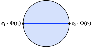
a. $(12)$

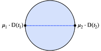
b. $[12]$

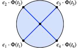
c. $(1234)$

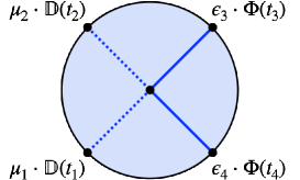
d. $[12|34)$

Figure 15: Four elementary Witten diagrams that we use to compute the two-point function with two charge $J$ scalars as well as the four-point functions with two charge $J$ scalars and two unit scalars or two unit displacement operators. a. scalar boundary-to-boundary propagator with one-loop correction (not depicted). b. displacement boundary-to-boundary propagator with one-loop correction (not depicted). c. four-point contact diagram with four legs incident on scalars. d. four-point contact diagram with two legs incident on scalars and two legs incident on displacment operators.

The third and fourth building blocks are the contact diagram with four external legs connected to elementary scalars and the contact diagram with two external legs connected to elementary scalars and two legs connected to elementary displacement operators. Due to the interaction vertex in the bulk, these are suppressed by $1/g$. We write the contact diagrams using the abbreviated notation,

$$(1234) \equiv\frac{(12)(34)}{4\pi g}\Lambda(\chi,\xi,\zeta), [12|34) \equiv\frac{[12](34)}{4\pi g}G_{\mathbb{D}\Phi}(\chi),$$ (D.3)

and depict them graphically as in Figure 15 c and Figure 15 d. Here,

$$\Lambda(\chi,\xi,\zeta) \equiv\biggr{[}G_{S}^{(1)}(\chi)-\frac{2}{5}G_{T}^{(1)}(\chi)+\xi\left(G_{T}^{(1)}(\chi)+G_{A}^{(1)}(\chi)\right)+\zeta\left(G_{T}^{(1)}(\chi)-G_{A}^{(1)}(\chi)\right)\biggr{]},$$ (D.4)

and the functions $G_{S}^{(1)}(\chi)$, $G_{T}^{(1)}(\chi)$ and $G_{A}^{(1)}(\chi)$ are given explicitly in [19]. Likewise, $G_{\mathbb{D}\Phi}(\chi)$ also follows from the results therein and is given explicitly by

$$G_{\mathbb{D}\Phi}(\chi)\equiv-4\left(1+\left(\frac{1}{\chi}-\frac{1}{2}\right)\log|1-\chi|\right).$$ (D.5)

Because $(\epsilon_{3}\cdot\Phi(t_{3}))^{J}$ and $(\epsilon_{4}\cdot\Phi(t_{4}))^{J}$ are composite operators, there will be also be diagrams in which one pair of legs of the scalar four-point contact diagram are incident on the same point, or two pairs of legs are incident on two points. When $\epsilon_{4}=\epsilon_{1}$ and $t_{4}\to t_{1}$, then $\xi=1$, $\zeta=0$, $\chi\to 1$, and therefore $\Lambda\to-3$. Thus, the scalar contact diagrams with one or two pairs of legs coincident simplify to

$$(1123) =-\frac{3}{4\pi g}(12)(13), (1122)=-\frac{3}{4\pi g}(12)^{2}.$$ (D.6)

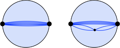
Figure 16: The Witten diagrams contributing to the two-point function $\braket{(\epsilon_{3}\cdot\Phi(t_{3}))^{J}(\epsilon_{4}\cdot\Phi(t_{4}))^{J}}$ to first subleading order in $1/g$ have two distinct topologies, corresponding to the two terms in (D.7).

Now we have everything necessary to determine the four-point correlators in (2.13)-(2.14), as well as the “heavy-heavy” two-point function they are normalized by, to subleading order. Let’s start with the heavy-heavy two-point function. The contributing Witten diagrams belong to one of two classes distinguished by their topologies, which are depicted in Figure 16. Keeping track of the combinatorial factors, we find

$$\braket{(\epsilon_{3}\cdot\Phi(t_{3}))^{J}(\epsilon_{4}\cdot\Phi(t_{4}))^{J}} =J!(34)^{J}+\binom{J}{2}^{2}(J-2)!(3344)(34)^{J-2}$$ (D.7)

$$=\left(\frac{2g}{\pi}\frac{\epsilon_{3}\cdot\epsilon_{4}}{t_{34}^{2}}\right)^{J}J!\left(1-\frac{3J(J+1)}{16\pi g}+O(1/g^{2})\right).$$ (D.8)

Second, the Witten diagrams contributing to the four-point function in (2.13) belong to one of six classes distinguished by their topologies, which are depicted in Figure 17. Permuting the two light operators and the two heavy operators, and keeping track of the appropriate combinatorial factors, we find

$$\braket{\epsilon_{1}\cdot\Phi(t_{1})\epsilon_{2}\cdot\Phi(t_{2})(\epsilon_{3}\cdot\Phi(t_{3}))^{J}(\epsilon_{4}\cdot\Phi(t_{4}))^{J}}=J!\left[(12)(34)+J(13)(24)+J(14)(23)\right](34)^{J-1}$$

$$\hskip 56.9055pt+\binom{J}{2}^{2}(J-2)!\left[(12)(34)+(J-2)(13)(24)+(J-2)(14)(23)\right](3344)(34)^{J-3}$$

$$\hskip 56.9055pt+\binom{J}{2}J!\left[(1344)(23)+(2344)(13)+(1334)(24)+(2334)(14)\right](34)^{J-2}$$

$$\hskip 56.9055pt+J!J(1234)(34)^{J-1}.$$ (D.9)

The first line above captures the contributions from the first two topologies in Figure 17; the second line captures the contributions from the third and fourth topologies; the third line captures the contributions from the fifth topology; and the last line captures the contribution from the sixth topology.

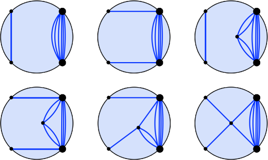
Figure 17: The Witten diagrams contributing to the four-point function $\braket{\epsilon_{1}\cdot\Phi(t_{1})\epsilon_{2}\cdot\Phi(t_{2})(\epsilon_{3}\cdot\Phi(t_{3}))^{J}(\epsilon_{4}\cdot\Phi(t_{4}))^{J}}$ to first subleading order in $1/g$ have six distinct topologies. There are eleven topologies ($=1+2+1+2+4+1$) if we distinguish between configurations with the light and heavy operators permuted. These correspond to the eleven terms in (D.9).

Given the explicit expressions for the propagators and the contact diagram in (D.1) and (D.3), the expression in (D.9) simplifies to

$$\braket{\epsilon_{1}\cdot\Phi(t_{1})\epsilon_{2}\cdot\Phi(t_{2})(\epsilon_{3}\cdot\Phi(t_{3}))^{J}(\epsilon_{4}\cdot\Phi(t_{4}))^{J}}=J!\left(\frac{2g}{\pi}\right)^{J+1}\frac{\epsilon_{1}\cdot\epsilon_{2}}{x_{12}^{2}}\frac{(\epsilon_{3}\cdot\epsilon_{4})^{J}}{x_{34}^{2J}}\biggr{[}1-\frac{3(J^{2}+J+2)}{16\pi g}$$

$$\hskip 85.35826pt+J\left(\xi\chi^{2}+\frac{\zeta\chi^{2}}{(1-\chi)^{2}}\right)\left(1-\frac{3J(J+3)}{16\pi g}\right)+\frac{J}{4\pi g}\Lambda+O(1/g^{2})\biggr{]}.$$ (D.10)

Thus, given (D.8), the normalized four-point function is

$$\frac{\braket{\epsilon_{1}\cdot\Phi(t_{1})\text{ }\epsilon_{2}\cdot\Phi(t_{2})(\epsilon_{3}\cdot\Phi(t_{3}))^{J}(\epsilon_{4}\cdot\Phi(t_{4}))^{J}}}{\frac{2g}{\pi}\frac{\epsilon_{1}\cdot\epsilon_{2}}{t_{12}^{2}}\braket{(\epsilon_{3}\cdot\Phi(t_{3}))^{J}(\epsilon_{4}\cdot\Phi(t_{4}))^{J}}}$$ (D.11)

$$\hskip 85.35826pt=1-\frac{3}{8\pi g}+J\left(\xi\chi^{2}+\frac{\zeta\chi^{2}}{(1-\chi)^{2}}\right)\left(1-\frac{3J}{8\pi g}\right)+\frac{J}{4\pi g}\Lambda(\xi,\zeta,\chi)+O(1/g^{2}),$$

and the three conformally invariant functions reduce to

$$G_{1}(\chi) =1-\frac{3}{8\pi g}+\frac{J}{4\pi g}\left(G_{S}^{(1)}-\frac{2}{5}G_{T}^{(1)}\right)+O(1/g^{2}),$$ (D.12)

$$G_{2}(\chi) =\frac{J\chi^{2}}{(1-\chi)^{2}}\left(1-\frac{3J}{8\pi g}\right)+\frac{J}{4\pi g}(G_{T}^{(1)}-G_{A}^{(1)})+O(1/g^{2}),$$ (D.13)

$$G_{3}(\chi) =J\chi^{2}\left(1-\frac{3J}{8\pi g}\right)+\frac{J}{4\pi g}(G_{T}^{(1)}+G_{A}^{(1)})+O(1/g^{2}).$$ (D.14)

We can thus identify the first few terms in the double expansion of the conformal functions in $1/g$ and $\mathcal{J}=J/g$. Using (5.16), we can also write the result as an expansion in $1/g$ and $c^{2}$. We find:

$$G_{1}(\chi) =\left(1+\frac{\mathcal{J}}{4\pi}\left(G_{S}^{(1)}-\frac{2}{5}G_{T}^{(1)}\right)+O(\mathcal{J}^{2})\right)+\frac{1}{g}\left(-\frac{3}{8\pi}+O(\mathcal{J})\right)+O(1/g^{2})$$

$$=\left(1+\frac{c^{2}}{4}\left(G_{S}^{(1)}-\frac{2}{5}G_{T}^{(1)}\right)+O(c^{4})\right)+\frac{1}{g}\left(-\frac{3}{8\pi}+O(c^{2})\right)+O(1/g^{2})$$ (D.15)

$$G_{2}(\chi) =\frac{g\chi^{2}}{(1-\chi)^{2}}\left(\mathcal{J}-\frac{3\mathcal{J}^{2}}{8\pi}+O(\mathcal{J}^{3})\right)+\left(\frac{\mathcal{J}}{4\pi}\left(G_{T}^{(1)}-G_{A}^{(1)}\right)+\mathcal{J}^{2}\right)+O(1/g)$$

$$=\frac{g\pi\chi^{2}}{(1-\chi)^{2}}\left(c^{2}+0c^{4}+O(c^{6})\right)+\left(\frac{c^{2}}{4}\left(G_{T}^{(1)}-G_{A}^{(1)}\right)+O(c^{4})\right)+O(1/g).$$ (D.16)

$$G_{3}(\chi) =g\chi^{2}\left(\mathcal{J}-\frac{3\mathcal{J}^{2}}{8\pi}+O(\mathcal{J}^{3})\right)+\left(\frac{\mathcal{J}}{4\pi}\left(G_{T}^{(1)}+G_{A}^{(1)}\right)+O(\mathcal{J}^{2})\ldots\right)+O(1/g)$$

$$=g\pi\chi^{2}\left(c^{2}+0c^{4}+O(c^{6})\right)+\left(\frac{c^{2}}{4}\left(G_{T}^{(1)}+G_{A}^{(1)}\right)+O(c^{4})\right)+O(1/g)$$ (D.17)

Given the explicit forms of $G_{S}^{(1)}(\chi)$, $G_{T}^{(1)}(\chi)$ and $G_{A}^{(1)}(\chi)$ from [19], we easily check that (D.15)-(D.17) precisely match the (5.21)-(5.23) in the overlapping terms.

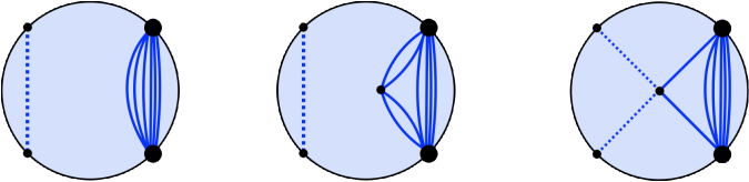
Figure 18: The Witten diagrams contributing to the four-point function $\braket{\mu_{1}\cdot\mathbb{D}(t_{1})\mu_{2}\cdot\mathbb{D}(t_{2})(\epsilon_{3}\cdot\Phi(t_{3}))^{J}(\epsilon_{4}\cdot\Phi(t_{4}))^{J}}$ to first subleading order in $1/g$ have three distinct topologies corresponding to the three terms in (D.18).

Finally, the Witten diagrams contributing to the four-point function in (2.14) belong to one of three classes distinguished by their topologies, which are depicted in Figure 18. Explicitly, we have

$$\braket{\mu_{1}\cdot\mathbb{D}(t_{1})\mu_{2}\cdot\mathbb{D}(t_{2})(\epsilon_{3}\cdot\Phi(t_{3}))^{J}(\epsilon_{4}\cdot\Phi(t_{4}))^{J}}$$

$$=J^{J}+\binom{J}{2}^{2}(J-2)(34)^{J-2}+J!J[12|34)(34)^{J-1}$$ (D.18)

$$=6J!\left(\frac{2g}{\pi}\right)^{J+1}\frac{\mu_{1}\cdot\mu_{2}}{t_{12}^{4}}\frac{(\epsilon_{3}\cdot\epsilon_{4})^{J}}{t_{34}^{2J}}\biggr{[}1-\frac{3(J^{2}+J+2)}{16\pi g}+\frac{J}{4\pi g}G_{\mathbb{D}\Phi}(\chi)+\ldots\biggr{]}.$$ (D.19)

The conformal function $G_{4}(\chi)$ is therefore:

$$G_{4}(\chi) =\frac{\braket{\mu_{1}\cdot\mathbb{D}(t_{1})\mu_{2}\cdot\mathbb{D}(t_{2})(\epsilon_{3}\cdot\Phi(t_{3}))^{J}(\epsilon_{4}\cdot\Phi(t_{4}))^{J}}}{\frac{12g}{\pi}\frac{\mu_{1}\cdot\mu_{2}}{t_{12}^{4}}(\epsilon_{3}\cdot\Phi(t_{3}))^{J}(\epsilon_{4}\cdot\Phi(t_{4}))^{J}}=1-\frac{3}{4\pi g}+\frac{J}{4\pi g}G_{\mathbb{D}\Phi}(\chi)+O(1/g^{2}),$$ (D.20)

which can also be written as an expansion in $1/g$ and $\mathcal{J}$ or $1/g$ and $c^{2}$:

$$G_{4}(\chi) =\left(1+\frac{\mathcal{J}}{4\pi}G_{\mathbb{D}\Phi}(\chi)+O(\mathcal{J}^{2})\right)+\frac{1}{g}\left(-\frac{3}{4\pi}+O(\mathcal{J})\right)+O(1/g^{2})$$

$$=\left(1+\frac{c^{2}}{4}G_{\mathbb{D}\Phi}(\chi)+O(c^{4})\right)+\frac{1}{g}\left(-\frac{3}{4\pi}+O(c^{2})\right)+O(1/g^{2}).$$ (D.21)

Given (D.5), this precisely matches (5.24) in the overlapping terms.

D.2 Finite charge OPE data

Next we extract OPE data from the finite charge four-point functions. Because the large charge and finite charge four-point functions agree in the regime of overlapping validity, the corresponding OPE data must necessarily agree as well. Nonetheless, the procedure we use in the present section to extract the finite charge OPE data is conceptually different from what we used in Section 5, and therefore provides additional insight and serves as a nice check of the large charge results.

Like in Section 5, we focus on the four-point function $\braket{ZZ^{J}\bar{Z}\bar{Z}^{J}}$ in the $12\to 34$ channel. (For brevity, we will not also consider $\braket{Z^{J}Z\bar{Z}\bar{Z}^{J}}$). From (5.11) combined with (D.12) and (D.13), we have

$$\braket{Z(t_{1})Z^{J}(t_{2})\bar{Z}(t_{3})\bar{Z}^{J}(t_{4})} =\frac{\mathcal{N}_{Z\bar{Z}}\mathcal{N}_{Z^{J}\bar{Z}^{J}}}{t_{21}^{J+1}t_{43}^{J+1}}\left(\frac{t_{42}}{t_{31}}\right)^{1-J}\chi^{J+1}\biggr{[}1+\frac{J}{(1-\chi)^{2}}+\frac{J}{4\pi g}\biggr{(}-\frac{3(J-1)}{2(1-\chi)^{2}}$$

$$+\left(G_{S}^{(1)}+\frac{3}{5}G_{T}^{(1)}-G_{A}^{(1)}\right)\biggr{\rvert}_{\chi^{-1}}\biggr{)}+O(1/g^{2})\biggr{]}.$$ (D.22)

We can again analyze this correlator using the conformal block expansion given in (5.1). With $J$ finite, we work perturbatively in $1/g$ instead of in $1/J$.

Constructing primaries out of generalized free fields.

In the strong coupling limit, $g\to\infty$, the Wilson line dCFT reduces to a generalized free field theory. Since $Z$ and $\bar{Z}$ behave like generalized free fields with unit conformal dimension, we can explicitly construct the conformal primaries appearing in the OPEs of $Z$ and $Z^{J}$ (and likewise in the OPE of $\bar{Z}$ and $\bar{Z}^{J}$) using the conformal algebra. Even though we can deduce OPE data using the conformal block expansion without needing to know the precise form of the exchanged operators, constructing at least the first few operators explicitly makes the analysis more transparent and illustrates some of the assumptions we made about the operators appearing in the conformal block expansions in Section 5.

In $1d$, the conformal algebra is given by $[K,P]=2D$, $[D,P]=P$, $[D,K]=-K$. Since $Z$ is a primary of dimension $1$, it satisfies $DZ=Z$ and $KZ=0$, and its descendants are $P^{m}Z$ for $m=1,2,3,\ldots$. We can construct additional primaries by taking linear combinations of the different ways that $m$ copies of $P$ can act on $J+1$ copies of $Z$. If $J$ is arbitrarily large, the number of different ways is equal to the number of ways, denoted $p_{m}$, to partition the positive integer $m$ into a sum of positive integers. The counting of partitions has a nice generating function: $\sum_{m=0}^{\infty}p_{m}q^{m}=\prod_{m=1}^{\infty}\frac{1}{1-q^{m}}=1+q+2q^{2}+3q^{3}+5q^{4}+7q^{5}+\ldots$. Since each operator can be written as a linear combination of primaries and descendants, it follows that the $p_{m}$-dimensional vector space spanned by the operators constructed out of $m$ copies of $P$ acting on $J+1$ copies of $Z$ has a $(p_{m}-p_{m-1})-$dimensional subspace spanned by primaries and a $p_{m-1}$-dimensional subspace spanned by descendants of the lower-$m$ primaries. The subspace of primaries is equivalently the space of solutions to $K\mathcal{O}=0$ at a given $m$.

For the sake of illustration, let us construct the first few primaries. We will denote them by $[Z^{J+1}]^{0}_{m,i}$ where $m$ denotes the number of copies of $P$, $i$ is a label to distinguish between degenerate primaries, if the space of solutions to $K\mathcal{O}=0$ has dimension greater than one, and the superscript $0$ indicates that these are the primaries in the generalized free field theory. Using $DP^{m}Z=(\Delta+m)P^{m}Z$ and $KP^{m}Z=m(m+2\Delta-1)P^{m-1}Z$, which follow from the conformal algebra, one can show that the following are conformal primaries

$$[Z^{J+1}]_{0} =Z^{J+1},$$ (D.23)

$$[Z^{J+1}]_{2} =Z^{J}P^{2}Z-\frac{3}{2}Z^{J-1}(PZ)^{2},$$ (D.24)

$$[Z^{J+1}]_{3} =Z^{J}P^{3}Z-6Z^{J-1}(P^{2}Z)(PZ)+6Z^{J-2}(PZ)^{3}$$ (D.25)

$$[Z^{J+1}]_{4,1} =Z^{J}P^{4}Z-10Z^{J-1}(P^{3}Z)(PZ)+10Z^{J-1}(P^{2}Z)^{2}$$ (D.26)

$$[Z^{J+1}]_{4,2} =Z^{J-1}(P^{2}Z)^{2}-3Z^{J-2}(P^{2}Z)(PZ)^{2}+\frac{9}{4}Z^{J-3}(PZ)^{4}.$$ (D.27)

In particular, they satisfy $K[Z^{J+1}]_{m,i}=0$ and $D[Z^{J+1}]_{m,i}=J+1+m$. These have not been normalized in any particular way and $[Z^{J+1}]_{4,1}$ and $[Z^{J+1}]_{4,2}$ form an arbitrary basis for the $2$-dimensional space of $m=4$ primaries.

If we were to continue the construction for larger $m$, we would find that the primaries with $m>4$ obey the following basic patterns:

• There is one conformal primary constructed out of $J+1$ copies of $Z$ (likewise $\bar{Z}$) at $m=0$, $m=2$, and $m=3$. There is more than one conformal primary constructed out of $J+1$ copies of $Z$ (likewise $\bar{Z}$) at each $m\geq 4$. There is no conformal primary at $m=1$.

• The dimensions of the primaries are $\Delta_{[Z^{J+1}]_{m,i}}=\Delta_{[\bar{Z}^{J+1}]_{m,i}}=J+1+m$. Moreover, under parity $[Z^{J+1}]_{m,i}$ and $[\bar{Z}^{J+1}]_{m,i}$ are odd if $m$ is odd and even if $m$ is even. This follows because $P\mathcal{O}=-i\partial\mathcal{O}$.

• We may choose the basis of primaries constructed out of $\bar{Z}$ so that they satisfy $[Z^{J+1}]_{m,i}^{\dagger}=[\bar{Z}^{J+1}]_{m,i}$. This follows from $[P,Z]^{\dagger}=-[P,\bar{Z}]$. Furthermore, applying a Gram-Schmidt-like procedure, using $\braket{Z(t_{1})\bar{Z}(t_{2})}=\frac{4g}{\pi}\frac{1}{t_{21}^{2}}$ and Wick contractions to evaluate the inner product $\braket{[Z^{J+1}]_{m,i}[\bar{Z}^{J+1}]_{m^{\prime},i^{\prime}}}$, we can construct an orthonormal basis that satisfies $\braket{[Z^{J+1}]_{m,i}[Z^{J+1}]_{m^{\prime},i^{\prime}}}=\braket{[\bar{Z}^{J+1}]_{m,i}[\bar{Z}^{J+1}]_{m^{\prime},i^{\prime}}}=0$ and $\braket{[Z^{J+1}]_{m,i}[\bar{Z}^{J+1}]_{m^{\prime},i^{\prime}}}=\delta_{mm^{\prime}}\delta_{ii^{\prime}}$.

Extracting OPE data.

Let us now return to the four-point function in (D.22). We will denote the conformal primaries contributing to the conformal block expansion by $[Z^{J+1}]_{m,i}$, which we have labelled based on the property that they reduce to the generalized free-field primaries at strong coupling: $[Z^{J+1}]_{m,i}\to[Z^{J+1}]^{0}_{m,i}$ as $g\to\infty$. In analogy with degenerate perturbation theory in quantum mechanics, this means choosing a basis $[Z^{J+1}]^{0}_{m,i}$ for each degenerate subspace with $m\geq 4$ that diagonalizes the interaction.

We expand the conformal dimensions and OPE coefficients of the primaries in $1/g$:

$$\Delta_{m,i} \equiv\Delta_{[Z^{J+1}]_{m,i}}=J+1+m+\frac{\gamma_{m,i}}{4\pi g}+O(1/g^{2}),$$ (D.28)

$$a_{m,i} \equiv\frac{\mathcal{C}_{ZZ^{J}[Z^{J+1}]_{m,i}}\mathcal{C}_{\bar{Z}\bar{Z}^{J}[\bar{Z}^{J+1}]_{m,i}}}{\mathcal{N}_{Z\bar{Z}}\mathcal{N}_{Z^{J}\bar{Z}^{J}}\mathcal{N}_{[Z^{J+1}]_{m,i}[\bar{Z}^{J+1}]_{m,i}}}=a_{m,i}^{0}+\frac{a_{m,i}^{1}}{4\pi g}+O(1/g^{2}).$$ (D.29)

Invoking (5.1), we can write the conformal block expansion of (D.22) and expand in $1/g$:

$$\braket{Z(t_{1})Z^{J}(t_{2})\bar{Z}(t_{3})\bar{Z}^{J}(t_{4})}=\frac{\mathcal{N}_{Z\bar{Z}}\mathcal{N}_{Z^{J}\bar{Z}^{J}}}{t_{21}^{J+1}t_{43}^{J+1}}\left(\frac{t_{42}}{t_{31}}\right)^{1-J}\sum_{m=0}^{\infty}\sum_{i\geq 1}a_{m,i}\chi^{\Delta_{m,i}}F_{\Delta_{m,i},J-1}(\chi)$$

$$=\frac{\mathcal{N}_{Z\bar{Z}}\mathcal{N}_{Z^{J}\bar{Z}^{J}}}{t_{21}^{J+1}t_{43}^{J+1}}\left(\frac{t_{42}}{t_{31}}\right)^{1-J}\sum_{m=0}^{\infty}\sum_{i\geq 1}\biggr{[}a_{m,i}^{0}\chi^{J+1+m}F_{J+1+m,J-1}(\chi)$$ (D.30)

$$\hskip 56.9055pt+\frac{\chi^{J+1+m}}{4\pi g}\left(a_{m,i}^{0}\gamma_{m,i}\log{\chi}+a_{m,i}^{1}+a_{m,i}^{0}\gamma_{m,i}\partial_{m}\right)F_{J+1+m,J-1}(\chi)+O(1/g^{2})\biggr{]},$$

where we introduced $F_{h,a}(\chi)\equiv{{}_{2}F_{1}}(h+a,h-a,2h,\chi)$ for shorthand.

By comparing the expansions in (D.30) and (D.22) and disentangling the different conformal blocks, we can extract information about $a_{m,i}^{0}$, $\gamma_{m,i}$ and $a_{m,i}^{1}$. Because $[Z^{J+1}]_{m,i}$ for each $i\geq 1$ have the same conformal dimension at leading order, the conformal block expansion does not distinguish between the different operators, and the OPE data that we can extract are the “operator-averaged” OPE coefficients and anomalous dimensions:

$$\bar{a}_{m}^{0} \equiv\sum_{i\geq 1}a_{m,i}^{0}, \bar{a}_{m}^{1}\equiv\sum_{i\geq 1}a_{m,i}^{1}, \bar{\gamma}_{m}\equiv\frac{1}{\bar{a}_{m}^{0}}\sum_{i\geq 1}a_{m,i}^{0}\gamma_{m,i}.$$ (D.31)

For simplicity, we will focus on $\bar{a}_{m}^{0}$ and $\bar{\gamma}_{m}$. To disentangle the conformal blocks, it is useful to note that they satisfy the following orthogonality relation:

$$\oint\frac{dz}{2\pi i}\frac{1}{z^{2}}z^{\Delta+m}F_{\Delta+m,a}(z)z^{1-\Delta-m^{\prime}}F_{1-\Delta-m^{\prime},a}(z)=\delta_{mm^{\prime}}.$$ (D.32)

This holds for any $a\in\mathbb{R}$, $\Delta=1,2,3,\ldots$ and $n,n^{\prime}=0,1,2,\ldots$. We also note

$$\oint\frac{dz}{2\pi i}\frac{1}{z^{2}}z^{-J-m}F_{-J-m,J-1}(z)z^{J+1} =(-1)^{m}\frac{\Gamma(2J+m)\Gamma(m+2)\Gamma(m+2J+1)}{\Gamma(2J)\Gamma(m+1)\Gamma(2m+2J+1)},$$ (D.33)

$$\oint\frac{dz}{2\pi i}\frac{1}{z^{2}}z^{-J-m}F_{-J-m,J-1}(z)\frac{z^{J+1}}{(1-z)^{2}} =\frac{\Gamma(m+2)^{2}\Gamma(m+2J+1)}{\Gamma(m+1)\Gamma(2m+2J+1)}.$$ (D.34)

Finally, comparing (D.30) with (D.22) at leading order, we have

$$\sum_{m=0}^{\infty}\bar{a}_{m}^{0}\chi^{J+1+m}F_{J+1+m,J-1}(\chi) =\chi^{J+1}\left(1+\frac{J}{(1-\chi)^{2}}\right).$$ (D.35)

Applying the orthogonality condition (D.32) and (D.33)-(D.34) yields

$$\bar{a}_{m}^{0} =\left(J\Gamma(2+m)\Gamma(2J)+(-1)^{m}\Gamma\left(2J+m\right)\right)\frac{(m+1)\Gamma\left(m+2J+1\right)}{\Gamma(2J)\Gamma(2m+2J+1)}.$$ (D.36)

Note that the RHS evaluates to zero $m=1$, reflecting the fact that there is no primary with $m=1$, as per the discussion around (D.23)-(D.27).

Next, if compare the term at order $1/g$ that is proportional to $\log{\chi}$, we have

$$\sum_{m=0}^{\infty}\bar{a}_{m}^{0}\bar{\gamma}_{m}\chi^{J+1+m}F_{J+1+m,J-1}(\chi) =\frac{J\chi^{J+1}}{4\pi g}\left[G_{S}^{(1)}(\chi^{-1})+\frac{3}{5}G_{T}^{(1)}(\chi^{-1})-G_{A}^{(1)}(\chi^{-1})\right]_{\log{\chi}}$$ (D.37)

The prefactors of the $\log{\chi}$ terms in $G_{S}^{(1)}$, $G_{T}^{(1)}$ and $G_{A}^{(1)}$ are rational functions that can be read off the explicit expressions in [19]. Using the orthogonality of the conformal blocks, we find

$$\bar{\gamma}_{m} =\frac{J}{\bar{a}_{m}^{0}}\oint\frac{d\chi}{2\pi i}\frac{1}{\chi^{2}}\chi^{-J-m}F_{-J-m,J-1}(\chi)\chi^{J+1}\frac{2\chi^{2}(3+\chi(\chi-3))}{(\chi-1)^{3}},$$ (D.38)

By evaluating the above contour integral analytically for a range of $J$ and $m$, we deduce the following simple expression for $\bar{\gamma}_{m}$:

$$\bar{\gamma}_{0} =0, \bar{\gamma}_{m} =-\frac{m(m+1)}{2}-Jm,\text{ for }m=2,3,\ldots.$$ (D.39)

Finally, we can compare the finite charge OPE data with the large charge OPE data. First, we identify the operators we denoted $[ZZ^{J}]_{n}$ in Section 5.1 with the operators $[Z^{J+1}]_{m}$ we defined in this section such that $n=0$ corresponds to $m=0$, and $n\geq 1$ corresponds to $m=n+1$. Then, expanding the finite charge OPE coefficients in $1/J$, we find for the $m=0$ and $m\geq 2$ operators:

$$\bar{a}_{0} =J+1+O(1/g)=g\left(\mathcal{J}+O(\mathcal{J}^{2})\right)+(1+O(\mathcal{J}))+O(1/g).$$ (D.40)

$$\ \bar{a}_{m} =\left[(-1)^{m}(m+1)+O(1/J)\right]+O(1/g).$$ (D.41)

Identifying $m=n+1$ for $n\geq 1$, we see that these expressions match (5.26)-(5.27) in the overlapping terms.

We can similarly expand the conformal dimensions in $1/g$ and $1/J$, we find for the $m=0$ and $m\geq 2$ operators:

$$\Delta_{0} =J+1+O(1/g^{2})$$ (D.42)

$$=g\left(\mathcal{J}+0\mathcal{J}^{2}+O(\mathcal{J}^{3})\right)+(1+0\mathcal{J}+O(\mathcal{J}^{2}))+1/g(0+O(\mathcal{J}))+O(1/g^{2})$$

$$\Delta_{n} =J+1+m-\frac{Jm}{4\pi g}-\frac{m(m+1)}{8\pi g}+O(1/g^{2})$$ (D.43)

$$=g\left(\mathcal{J}+0\mathcal{J}^{2}+O(\mathcal{J}^{3})\right)+(m+1-\frac{m\mathcal{J}}{4\pi}+O(\mathcal{J}^{2}))+\frac{1}{g}\left(-\frac{m(m+1)}{8\pi}+O(\mathcal{J})\right)+O(1/g^{2}),$$

We find agreement with (5.42), including the absence of an operator with leading dimension $\Delta=J+2$. The fact that the agreement in the overlapping terms is exact reinforces the suggestion in Section 5 that operator mixing may not be relevant for the OPE data in the large charge limit.

References

- [1] Y. M. Makeenko and A. A. Migdal, “Exact Equation for the Loop Average in Multicolor QCD,” Phys. Lett. B 88 (1979) 135. [Erratum: Phys.Lett.B 89, 437 (1980)].
- [2] Y. Makeenko and A. A. Migdal, “Quantum Chromodynamics as Dynamics of Loops,” Sov. J. Nucl. Phys. 32 (1980) 431.
- [3] S. Giombi and S. Komatsu, “Loop equation and exact soft anomalous dimension in = 4 super Yang-Mills,” JHEP 06 (2020) 075, 2003.04460.
- [4] V. A. Kazakov and I. K. Kostov, “NONLINEAR STRINGS IN TWO-DIMENSIONAL U(INFINITY) GAUGE THEORY,” Nucl. Phys. B 176 (1980) 199–215.
- [5] V. A. Kazakov, “WILSON LOOP AVERAGE FOR AN ARBITRARY CONTOUR IN TWO-DIMENSIONAL U(N) GAUGE THEORY,” Nucl. Phys. B 179 (1981) 283–293.
- [6] M. Bianchi, M. B. Green, and S. Kovacs, “Instanton corrections to circular Wilson loops in N=4 supersymmetric Yang-Mills,” JHEP 04 (2002) 040, hep-th/0202003.
- [7] A. Kapustin, “Wilson-’t Hooft operators in four-dimensional gauge theories and S-duality,” Phys. Rev. D 74 (2006) 025005, hep-th/0501015.
- [8] N. Drukker and S. Kawamoto, “Small deformations of supersymmetric Wilson loops and open spin-chains,” JHEP 07 (2006) 024, hep-th/0604124.
- [9] M. Billò, V. Gonçalves, E. Lauria, and M. Meineri, “Defects in conformal field theory,” JHEP 04 (2016) 091, 1601.02883.
- [10] P. Liendo, C. Meneghelli, and V. Mitev, “Bootstrapping the half-BPS line defect,” JHEP 10 (2018) 077, 1806.01862.
- [11] P. Ferrero and C. Meneghelli, “Bootstrapping the half-BPS line defect CFT in N=4 supersymmetric Yang-Mills theory at strong coupling,” Phys. Rev. D 104 (2021), no. 8 L081703, 2103.10440.
- [12] J. Barrat, A. Gimenez-Grau, and P. Liendo, “Bootstrapping holographic defect correlators in super Yang-Mills,” 2108.13432.
- [13] A. Cavaglià, N. Gromov, J. Julius, and M. Preti, “Integrability and conformal bootstrap: One dimensional defect conformal field theory,” Phys. Rev. D 105 (2022), no. 2 L021902, 2107.08510.
- [14] S. Giombi and S. Komatsu, “Exact Correlators on the Wilson Loop in SYM: Localization, Defect CFT, and Integrability,” JHEP 05 (2018) 109, 1802.05201. [Erratum: JHEP11,123(2018)].
- [15] S. Giombi and S. Komatsu, “More Exact Results in the Wilson Loop Defect CFT: Bulk-Defect OPE, Nonplanar Corrections and Quantum Spectral Curve,” J. Phys. A 52 (2019), no. 12 125401, 1811.02369.
- [16] S. Giombi, J. Jiang, and S. Komatsu, “Giant Wilson loops and AdS2/dCFT1,” JHEP 11 (2020) 064, 2005.08890.
- [17] S. Giombi and V. Pestun, “Correlators of local operators and 1/8 BPS Wilson loops on S**2 from 2d YM and matrix models,” JHEP 10 (2010) 033, 0906.1572.
- [18] S. Giombi and V. Pestun, “Correlators of Wilson Loops and Local Operators from Multi-Matrix Models and Strings in AdS,” JHEP 01 (2013) 101, 1207.7083.
- [19] S. Giombi, R. Roiban, and A. A. Tseytlin, “Half-BPS Wilson loop and AdS2/CFT1,” Nucl. Phys. B922 (2017) 499–527, 1706.00756.
- [20] N. Drukker, “Integrable Wilson loops,” JHEP 10 (2013) 135, 1203.1617.
- [21] D. Correa, J. Maldacena, and A. Sever, “The quark anti-quark potential and the cusp anomalous dimension from a TBA equation,” JHEP 08 (2012) 134, 1203.1913.
- [22] N. Gromov and F. Levkovich-Maslyuk, “Quark-anti-quark potential in 4 SYM,” JHEP 12 (2016) 122, 1601.05679.
- [23] D. Grabner, N. Gromov, and J. Julius, “Excited States of One-Dimensional Defect CFTs from the Quantum Spectral Curve,” JHEP 07 (2020) 042, 2001.11039.
- [24] M. Kim and N. Kiryu, “Structure constants of operators on the Wilson loop from integrability,” JHEP 11 (2017) 116, 1706.02989.
- [25] N. Kiryu and S. Komatsu, “Correlation Functions on the Half-BPS Wilson Loop: Perturbation and Hexagonalization,” JHEP 02 (2019) 090, 1812.04593.
- [26] B. Basso, S. Komatsu, and P. Vieira, “Structure Constants and Integrable Bootstrap in Planar N=4 SYM Theory,” 1505.06745.
- [27] T. Fleury and S. Komatsu, “Hexagonalization of Correlation Functions,” JHEP 01 (2017) 130, 1611.05577.
- [28] B. Eden and A. Sfondrini, “Tessellating cushions: four-point functions in = 4 SYM,” JHEP 10 (2017) 098, 1611.05436.
- [29] N. Gromov, V. Kazakov, S. Leurent, and D. Volin, “Quantum Spectral Curve for Planar Super-Yang-Mills Theory,” Phys. Rev. Lett. 112 (2014), no. 1 011602, 1305.1939.
- [30] M. Kim, N. Kiryu, S. Komatsu, and T. Nishimura, “Structure Constants of Defect Changing Operators on the 1/2 BPS Wilson Loop,” JHEP 12 (2017) 055, 1710.07325.
- [31] M. Cooke, A. Dekel, and N. Drukker, “The Wilson loop CFT: Insertion dimensions and structure constants from wavy lines,” J. Phys. A 50 (2017), no. 33 335401, 1703.03812.
- [32] J. Barrat, P. Liendo, and J. Plefka, “Two-point correlator of chiral primary operators with a Wilson line defect in = 4 SYM,” JHEP 05 (2021) 195, 2011.04678.
- [33] J. Barrat, P. Liendo, G. Peveri, and J. Plefka, “Multipoint correlators on the supersymmetric Wilson line defect CFT,” 2112.10780.
- [34] J. Polchinski and J. Sully, “Wilson Loop Renormalization Group Flows,” JHEP 10 (2011) 059, 1104.5077.
- [35] M. Beccaria, S. Giombi, and A. Tseytlin, “Non-supersymmetric Wilson loop in = 4 SYM and defect 1d CFT,” JHEP 03 (2018) 131, 1712.06874.
- [36] M. Beccaria, S. Giombi, and A. A. Tseytlin, “Correlators on non-supersymmetric Wilson line in SYM and AdS2/CFT1,” JHEP 05 (2019) 122, 1903.04365.
- [37] M. Beccaria, S. Giombi, and A. A. Tseytlin, “Higher order RG flow on the Wilson line in = 4 SYM,” JHEP 01 (2022) 056, 2110.04212.
- [38] M. Beccaria, S. Giombi, and A. A. Tseytlin, “Wilson loop in general representation and RG flow in 1d defect QFT,” 2202.00028.
- [39] G. Cuomo, Z. Komargodski, M. Mezei, and A. Raviv-Moshe, “Spin Impurities, Wilson Lines and Semiclassics,” 2202.00040.
- [40] G. Cuomo, Z. Komargodski, and A. Raviv-Moshe, “Renormalization Group Flows on Line Defects,” Phys. Rev. Lett. 128 (2022), no. 2 021603, 2108.01117.
- [41] S. Giombi, S. Komatsu, and B. Offertaler, “Large Charges on the Wilson Loop in SYM: Matrix Model and Classical String,” 2110.13126.
- [42] S. Hellerman, D. Orlando, S. Reffert, and M. Watanabe, “On the CFT Operator Spectrum at Large Global Charge,” JHEP 12 (2015) 071, 1505.01537.
- [43] A. Monin, D. Pirtskhalava, R. Rattazzi, and F. K. Seibold, “Semiclassics, Goldstone Bosons and CFT data,” JHEP 06 (2017) 011, 1611.02912.
- [44] L. Alvarez-Gaume, O. Loukas, D. Orlando, and S. Reffert, “Compensating strong coupling with large charge,” JHEP 04 (2017) 059, 1610.04495.
- [45] S. Hellerman, S. Maeda, and M. Watanabe, “Operator Dimensions from Moduli,” JHEP 10 (2017) 089, 1706.05743.
- [46] S. Hellerman and S. Maeda, “On the Large -charge Expansion in Superconformal Field Theories,” JHEP 12 (2017) 135, 1710.07336.
- [47] L. A. Gaumé, D. Orlando, and S. Reffert, “Selected topics in the large quantum number expansion,” Phys. Rept. 933 (2021) 2180, 2008.03308.
- [48] D. Jafferis, B. Mukhametzhanov, and A. Zhiboedov, “Conformal Bootstrap At Large Charge,” JHEP 05 (2018) 043, 1710.11161.
- [49] A. Miwa and T. Yoneya, “Holography of Wilson-loop expectation values with local operator insertions,” Journal of High Energy Physics 2006 (2006) 060–060.
- [50] N. Gromov and A. Sever, “Analytic Solution of Bremsstrahlung TBA,” JHEP 11 (2012) 075, 1207.5489.
- [51] V. A. Kazakov, A. Marshakov, J. A. Minahan, and K. Zarembo, “Classical/quantum integrability in AdS/CFT,” JHEP 05 (2004) 024, hep-th/0402207.
- [52] N. Beisert, V. A. Kazakov, K. Sakai, and K. Zarembo, “The Algebraic curve of classical superstrings on AdS(5) x S**5,” Commun. Math. Phys. 263 (2006) 659–710, hep-th/0502226.
- [53] N. Gromov, S. Schafer-Nameki, and P. Vieira, “Efficient precision quantization in AdS/CFT,” JHEP 12 (2008) 013, 0807.4752.
- [54] J. Qiao and S. Rychkov, “A tauberian theorem for the conformal bootstrap,” JHEP 12 (2017) 119, 1709.00008.
- [55] D. Gaiotto, D. Mazac, and M. F. Paulos, “Bootstrapping the 3d Ising twist defect,” JHEP 03 (2014) 100, 1310.5078.
- [56] G. Sizov and S. Valatka, “Algebraic Curve for a Cusped Wilson Line,” JHEP 05 (2014) 149, 1306.2527.
- [57] D. Correa, J. Henn, J. Maldacena, and A. Sever, “An exact formula for the radiation of a moving quark in N=4 super Yang Mills,” JHEP 06 (2012) 048, 1202.4455.
- [58] D. Mazac and M. F. Paulos, “The analytic functional bootstrap. Part II. Natural bases for the crossing equation,” JHEP 02 (2019) 163, 1811.10646.
- [59] D. Z. Freedman, S. D. Mathur, A. Matusis, and L. Rastelli, “Correlation functions in the CFT(d) / AdS(d+1) correspondence,” Nucl. Phys. B546 (1999) 96–118, hep-th/9804058.
- [60] V. Forini, V. G. M. Puletti, L. Griguolo, D. Seminara, and E. Vescovi, “Remarks on the geometrical properties of semiclassically quantized strings,” J. Phys. A 48 (2015), no. 47 475401, 1507.01883.
- [61] N. Drukker, D. J. Gross, and A. A. Tseytlin, “Green-Schwarz string in AdS(5) x S**5: Semiclassical partition function,” JHEP 04 (2000) 021, hep-th/0001204.
- [62] M. Beccaria, G. V. Dunne, V. Forini, M. Pawellek, and A. A. Tseytlin, “Exact computation of one-loop correction to energy of spinning folded string in x ,” J. Phys. A 43 (2010) 165402, 1001.4018.
- [63] M. Beccaria, G. V. Dunne, G. Macorini, A. Tirziu, and A. A. Tseytlin, “Exact computation of one-loop correction to energy of pulsating strings in ,” J. Phys. A 44 (2011) 015404, 1009.2318.
- [64] V. Forini, “Quark-antiquark potential in AdS at one loop,” JHEP 11 (2010) 079, 1009.3939.
- [65] N. Drukker and V. Forini, “Generalized quark-antiquark potential at weak and strong coupling,” JHEP 06 (2011) 131, 1105.5144.
- [66] D. Pappadopulo, S. Rychkov, J. Espin, and R. Rattazzi, “OPE Convergence in Conformal Field Theory,” Phys. Rev. D 86 (2012) 105043, 1208.6449.
- [67] M. Hogervorst and S. Rychkov, “Radial Coordinates for Conformal Blocks,” Phys. Rev. D 87 (2013) 106004, 1303.1111.
- [68] D. F. Lawden, Elliptic functions and applications, vol. 80 of Applied Mathematical Sciences. Springer-Verlag, New York, 1989.
- [69] F. A. Dolan and H. Osborn, “Conformal Partial Waves: Further Mathematical Results,” 1108.6194.
- [70] N. M. Temme, “Large parameter cases of the Gauss hypergeometric function,” Journal of computational and applied mathematics 153 (2003), no. 1-2 441–462.
- [71] M. Nirschl and H. Osborn, “Superconformal Ward identities and their solution,” Nuclear Physics B 711 (2005), no. 3 409–479.
- [72] S. Schafer-Nameki, “Review of AdS/CFT Integrability, Chapter II.4: The Spectral Curve,” Lett. Math. Phys. 99 (2012) 169–190, 1012.3989.
- [73] N. Dorey and B. Vicedo, “On the dynamics of finite-gap solutions in classical string theory,” JHEP 07 (2006) 014, hep-th/0601194.
- [74] M. Abramowitz, I. A. Stegun, and R. H. Romer, “Handbook of mathematical functions with formulas, graphs, and mathematical tables,” 1988.
- [75] “NIST Digital Library of Mathematical Functions.” http://dlmf.nist.gov/, Release 1.1.3 of 2021-09-15. F. W. J. Olver, A. B. Olde Daalhuis, D. W. Lozier, B. I. Schneider, R. F. Boisvert, C. W. Clark, B. R. Miller, B. V. Saunders, H. S. Cohl, and M. A. McClain, eds.
- [76] E. T. Whittaker and G. N. Watson, A Course of Modern Analysis. Cambridge Mathematical Library. Cambridge University Press, 4 ed., 1996.
- [77] E. M. Stein and R. Shakarchi, Complex analysis, vol. 2. Princeton University Press, 2010.
- [78] Z. Bajnok, M. Kim, and L. Palla, “Spectral curve for open strings attached to the Y=0 brane,” JHEP 04 (2014) 035, 1311.7280.
- [79] R. A. Janik and A. Wereszczynski, “Correlation functions of three heavy operators: The AdS contribution,” JHEP 12 (2011) 095, 1109.6262.
- [80] Y. Kazama and S. Komatsu, “On holographic three point functions for GKP strings from integrability,” JHEP 01 (2012) 110, 1110.3949. [Erratum: JHEP 06, 150 (2012)].
- [81] Y. Kazama and S. Komatsu, “Three-point functions in the SU(2) sector at strong coupling,” JHEP 03 (2014) 052, 1312.3727.
- [82] Y. Kazama, S. Komatsu, and T. Nishimura, “Classical Integrability for Three-point Functions: Cognate Structure at Weak and Strong Couplings,” JHEP 10 (2016) 042, 1603.03164. [Erratum: JHEP 02, 047 (2018)].
- [83] K. Zarembo, “Holographic three-point functions of semiclassical states,” JHEP 09 (2010) 030, 1008.1059.
- [84] M. S. Costa, R. Monteiro, J. E. Santos, and D. Zoakos, “On three-point correlation functions in the gauge/gravity duality,” JHEP 11 (2010) 141, 1008.1070.
- [85] B. Vicedo, “Semiclassical Quantisation of Finite-Gap Strings,” JHEP 06 (2008) 086, 0803.1605.
- [86] A. Cavaglià, N. Gromov, and F. Levkovich-Maslyuk, “Quantum spectral curve and structure constants in SYM: cusps in the ladder limit,” JHEP 10 (2018) 060, 1802.04237.
- [87] A. Cavaglià, N. Gromov, and F. Levkovich-Maslyuk, “Separation of variables in AdS/CFT: functional approach for the fishnet CFT,” JHEP 06 (2021) 131, 2103.15800.
- [88] K. Zarembo, “Open string fluctuations in AdS(5) x S**5 and operators with large R charge,” Phys. Rev. D 66 (2002) 105021, hep-th/0209095.
- [89] T. Enari and A. Miwa, “Semi-classical correlator for 1/4 BPS Wilson loop and chiral primary operator with large R-charge,” Phys. Rev. D 86 (2012) 106004, 1208.0821.
- [90] N. Drukker, S. Giombi, R. Ricci, and D. Trancanelli, “On the D3-brane description of some 1/4 BPS Wilson loops,” JHEP 04 (2007) 008, hep-th/0612168.
- [91] B. Basso and D.-L. Zhong, “Three-point functions at strong coupling in the BMN limit,” JHEP 04 (2020) 076, 1907.01534.
- [92] A. Bourget, D. Rodriguez-Gomez, and J. G. Russo, “A limit for large -charge correlators in theories,” JHEP 05 (2018) 074, 1803.00580.
- [93] A. Grassi, Z. Komargodski, and L. Tizzano, “Extremal correlators and random matrix theory,” JHEP 04 (2021) 214, 1908.10306.
- [94] E. I. Buchbinder and A. A. Tseytlin, “Semiclassical four-point functions in x ,” JHEP 02 (2011) 072, 1012.3740.
- [95] J. Caetano and J. Escobedo, “On four-point functions and integrability in N=4 SYM: from weak to strong coupling,” JHEP 09 (2011) 080, 1107.5580.
- [96] H. Braden, “Periodic functional determinants,” Journal of Physics A: Mathematical and General 18 (1985), no. 12 2127–2140.
- [97] K. Roumpedakis, “Leading Order Anomalous Dimensions at the Wilson-Fisher Fixed Point from CFT,” JHEP 07 (2017) 109, 1612.08115.