Measuring frequency and period separations in red-giant stars using machine learning

Abstract

Asteroseismology is used to infer the interior physics of stars. The Kepler and TESS space missions have provided a vast data set of red-giant light curves, which may be used for asteroseismic analysis. These data sets are expected to significantly grow with future missions such as PLATO, and efficient methods are therefore required to analyze these data rapidly. Here, we describe a machine learning algorithm that identifies red giants from the raw oscillation spectra and captures p and mixed mode parameters from the red-giant power spectra. We report algorithmic inferences for large frequency separation ($\Delta\nu$), frequency at maximum amplitude ($\nu_{max}$), and period separation ($\Delta\Pi$) for an ensemble of stars. In addition, we have discovered $\sim$25 new probable red giants among 151,000 Kepler long-cadence stellar-oscillation spectra analyzed by the method, among which four are binary candidates which appear to possess red-giant counterparts. To validate the results of this method, we selected $\sim$ 3,000 Kepler stars, at various evolutionary stages ranging from subgiants to red clumps, and compare inferences of $\Delta\nu$, $\Delta\Pi$, and $\nu_{max}$ with estimates obtained using other techniques. The power of the machine-learning algorithm lies in its speed: it is able to accurately extract seismic parameters from 1,000 spectra in $\sim$5 seconds on a modern computer.

1 Introduction

Asteroseismology is an important tool that sheds light on stellar physics, allowing us to understand their inner structure and evolution. Space-borne instruments such as CoRoT (Baglin et al., 2006), Kepler (Borucki et al., 2004, 2010), and TESS (Ricker et al., 2015) have observed hundreds of thousands of stars and detected stellar pulsations in tens of thousands of them. Most of these pulsating stars are red giants (Mosser et al., 2010 a; Yu et al., 2018). Red giants are evolved solar-like stars, and, as in the Sun, pulsations are driven by turbulence in the outer layers of the convection zone. In most of those stars, only a few seismic characteristics have been identified (Bugnet et al., 2018; Hon et al., 2019).

Detailed studies of red giants have significantly improved our understanding of the interiors and evolution of stars (Bedding et al., 2011; Mosser et al., 2014). It also helped in probing their rotation (Beck et al., 2012; Deheuvels et al., 2014; Mauro et al., 2016), showing potential indications for strong magnetic fields in their inner layers (Fuller et al., 2015). Extending these detailed analyses to a broader range of stars (if not all solar-like stars) is necessary to deepen our understanding of stellar evolution and important processes such as angular momentum transport (Aerts et al., 2019).

In order to detect stellar pulsations, power spectra (squared absolute values of Fourier transforms of these recorded lightcurves) are typically analyzed. The spectra typically show a sequence of peaks rising above a noisy background, with each peak corresponding to a globally oscillatory mode that may be characterized using three quantum numbers, radial order $n$, harmonic degree $\ell$, and azimuthal order $m$. The primary challenge is then to identify and label the peaks accurately. In red giants, this task can be difficult and time consuming if one performs it by visual inspection of the spectrum. Although semi-automated approaches have been developed (Vrard et al., 2016; Gehan et al., 2018; Kallinger, 2019), the visual method remains common. Labeling allows to define appropriate assumptions in order to extract properties of modes such as the frequency, amplitude and width, generally using a fitting algorithm (Vrard et al., 2018). These parameters depend on the physical properties of the layers traversed by the modes, allowing us to infer the interior structure and rotation rates.

Current fitting methods to extract modes parameters in evolved stars e.g., (Benomar et al., 2009; Handberg & Campante, 2011; Corsaro & De Ridder, 2014) are relatively slow. This explains why only a small fraction of solar-like stars have been so far analyzed in details. To achieve a better understanding of stars in this era of ever-growing data, one needs efficient, much faster yet robust ways to measure features within the data that capture important physical information.

Machine learning has emerged as a powerful tool with which to identify patterns in complex data sets. Here, we develop a machine learning algorithm that allows us to perform mode identification in one single extremely fast step, mimicking current fitting methods. In standard fitting methods, each star is individually analyzed (in some cases each mode); in contrast, machine learning enables the analysis of ensembles of stars at once, making it computationally efficient.

In this article, we address the problem of measuring seismic parameters related to the structure of red giants using machine learning. Three seismic parameters are mainly involved - (a) large frequency separation ($\Delta\nu$), i.e., the average frequency spacing of $p$ - modes, (b) $\nu_{max}$, the $p$ - mode frequency at maximum power and (c) large-period separation ($\Delta\Pi$), i.e., the average period spacing of $g$ - modes. These parameters ($\Delta\nu$,$\nu_{max}$) are strongly correlated with mass and radius according to established scaling relations (Kippenhahn et al., 2012; Brown et al., 1991; Mathur et al., 2012). Along with this, the parameters ($\Delta\nu$, $\Delta\Pi$) separate the evolutionary stages of the star (Mosser et al., 2014) - (i) subgiant, Hydrogen depletion phase in the core, (ii) red giant branch, the phase of H-burning in the shell (iii) red clump, the phase of He-burning in low-mass stars and (iv) secondary red clump, the phase of He-burning in high-mass stars.

2 Results on real data

The success of machine learning entirely depends on the quality of the training data set. For the machine to detect a pattern and correctly predict a parameter in real data, we have modelled a synthetic data set that is realistic and that is able to account for typical variations in observations is required. We have incorporated the physics of structure, composition gradient, and rotation in red giants in our simulations using asymptotic theory of oscillations (García & Ballot, 2019; Aerts et al., 2010). The detailed modelling of the synthetic data is given in the Appendix A. To construct the periodograms of Kepler data, we use the MAST data from which we extract the PDCSAP light-curves (Stumpe et al., 2012; Smith et al., 2012), to which we fit a $6^{\mathrm{th}}$ order polynomial function in order to remove remaining trends in each quarter. Following this, quarters are concatenated and data points that lie beyond 3.5$\sigma$ of the mean are discarded in order to filter out spurious data points. This post-processed light-curve is then used to compute the Lomb-Scargle periodogram (Lomb, 1976; Scargle, 1982) following the Rybicki Press algorithm (Rybicki & Press, 1995) prescription to calculate the Nyquist frequency.

We have trained neural networks to perform four different tasks. The first task being the detection of red giants and the other three measure the respective seismic parameters ($\Delta\nu$,$\nu_{max}$,$\Delta\Pi$). Although these networks are different, the architecture of these networks remain the same. We have built the network on a base of the Convolutional Neural Network. Figure 1 shows the simplified architecture of the network, which takes a Normalized spectrum as an input and returns the inference of the seismic parameter. In the case of detection, the machine estimates the probability of Red-giant in the power spectrum. Additional details of the Machine learning model are provided in the Appendix A.

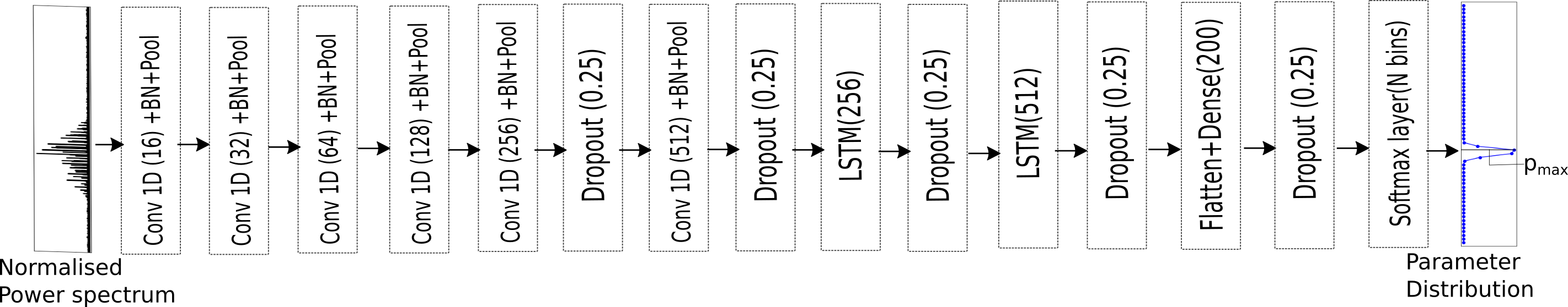
Figure 1: Architecture of neural network used in our machine learning algorithm. The network takes as input the (1D) normalized spectrum and outputs an approximate probability distribution of the subject parameter. $p_{max}$ in the inference of output shows the maximum probability (confidence) of the prediction. The core network is built using CNN, LSTM and Dense layers. Dropout layers with a fraction of 0.25 are used to prevent overfitting. The detailed network is presented in the Figure A.3

Table 1: Range of seismic parameters for the preparation of synthetic data.

Parameter	Subgiant	Young red giant branch	Old red giant branch	Red clumps
		(High-frequency red giants)	(Low-frequency red giants)
Range of $\Delta\nu$	18-50 $\mu$Hz	9-18 $\mu$Hz	6-9 $\mu$Hz	4.2-12 $\mu$Hz
Range of $\Delta\Pi$	60-200s	45-150s	45-110s	150-500s

Note. — This table shows the range of seismic parameters that were chosen to create different synthetic data sets. This range of parameters is chosen so as to cover the space of published results on Kepler Data Mosser et al. (2015); Vrard et al. (2016); Mosser et al. (2017). The detailed parameters used to create our simulations are shown in Table A.1.

We first demonstrate that the machine can distinguish red-giant oscillation spectra from noise, allowing us to discover new red-giant stars from the Kepler long cadence data set. We then validate machine inferences on Kepler data and finally illustrate that the machine can identify the relationship between the seismic parameters.

2.1 Machine-enabled detection of red giants

Figure 2: (a) Oscillation spectrum of a noisy spectrum KIC 12457108. (b) Oscillation spectrum of a red-giant KIC 5007487.

We first ensure that the machine is able to identify red-giant oscillation spectra. For this task, we have produced 500,000 synthetic data samples to train the neural network. The samples comprise an equal number of pure-noise and red-giant spectra, with a $\Delta\nu$ distribution of 1-18.7 $\mu$Hz and $\Delta\Pi$ ranging from 45-500s. Table A.1 shows the ranges of the seismic parameters in red-giant and noise simulations used to prepare the synthetic datasets. We then train the neural network to classify these samples. Figure 2 shows examples of two stars, one in which the spectra is dominated by noise (left) and another one in which the p-mode envelope is clearly visible (right). It shows that detection probability is low when the input is noise, whereas the network produces high probability for the p-mode envelope. If probability exceeds 0.5, we consider it to be a potential red giant.

We apply this method to identify red giants from the ensemble of 151,000 Kepler stars. Among these, 21,291 stars have been independently identified as red giants (Hekker et al., 2010; Stello et al., 2013; Pinsonneault et al., 2014; Mathur et al., 2016; Yu et al., 2018; Pinsonneault et al., 2018; Elsworth et al., 2019; Gaulme et al., 2020; Yu et al., 2020; Benbakoura et al., 2021; Mosser et al., 2015; Vrard et al., 2016; Mosser et al., 2017; Hon et al., 2019), out of which 17,527 stars are detected. Among other 130,288 stars not identified as pulsating red giants, 22,850 have been classified as positives. Thus, the algorithm shows 82.3% and 17.5% true and false-positive rates, respectively. Among these false positives, $\sim 50\%$ of stars are non-solar-like pulsators, such as rapidly rotating, $\delta$-scuti, $\Gamma$-Doradus stars, etc. Thus, the false positive rate associated with mislabelling noise as red giant oscillations is $\sim$ 8%. As part of future work, we will extend the preparation of synthetic datasets for non-solar-like pulsators to identify and categorize these stars.

After visual inspection, we detect $\sim$25 new likely red giants using this method, shown in Table C.1. We have explored various catalogues: Hekker et al. (2010); Stello et al. (2013); Pinsonneault et al. (2014); Mathur et al. (2016); Yu et al. (2018); Pinsonneault et al. (2018); Elsworth et al. (2019); Gaulme et al. (2020); Yu et al. (2020); Benbakoura et al. (2021); Mosser et al. (2015); Vrard et al. (2016); Mosser et al. (2017); Hon et al. (2019) to confirm that these 25 giant stars are new. We have provided the first measurements of $\Delta\nu$, $\Delta\Pi$, and $\nu_{max}$ for these stars in Table C.1. Table C.2 provides the first measurements of $\Delta\nu$ and $\Delta\Pi$ for 195 stars, which were detected by Hon et al. (2019).

We thus establish that the machine can identify red giants. In the next subsection, we validate the seismic-parameter inferences by comparing them to other methods (Mosser et al., 2015; Vrard et al., 2016; Mosser et al., 2017). For this purpose, we show the results of machine inferences in 3,029 stars. We chose these stars as these are the only stars in Mosser et al. (2015); Vrard et al. (2016); Mosser et al. (2017) that fall into the parameter space of the training dataset shown in Table 1 and have reliable estimates of all the period-spacing parameters.

2.2 Results of machine inferences

We have divided our synthetic training dataset into four subsets which indicate different evolutionary stages as given in Table 1. For each stellar class given in Table 1, we train the machine separately, leaving four different machines for each parameter, where the core networks are identical but the final layers change in accordance with the parameter and resolution required. Once trained, the neural network’s performance is evaluated on a test data set, which comprises the unseen synthetic data. We show machine can infer $\Delta\nu$, $\nu_{max}$ and $\Delta\Pi$ successfully on this data set in Appendix B.

To corroborate the deep-learning method, it is essential to verify the results from the neural network and compare them with estimates obtained using independent methods. We show that the trained machine can identify oscillation modes of Kepler red giants. Though we have neural network outputs for 151,000 stars, for this analysis, we have selected 3,029 red giants from Mosser et al. (2014); Vrard et al. (2016) to allow a qualitative comparison between this work and other methods. Based on results from their analyses, we have categorized this 3,000-star sample into our four stellar classes: subgiants ($\Delta\nu$: 18-50$\mu$Hz), young red giant branch ($\Delta\nu$: 9-18$\mu$Hz), old red giant branch ($\Delta\nu$: 6-9$\mu$Hz, $\Delta\Pi$$<$150s), and red clumps ($\Delta\nu$: 4.2-12$\mu$Hz, $\Delta\Pi$$>$150s). We show the performance of neural networks corresponding to each stellar class.

Figure 3(a) depicts neural-network predictions against the published values (Mosser et al., 2014; Vrard et al., 2016) of $\Delta\nu$ in each stellar class. Figure 3(b) shows the distribution of relative differences between published values and corresponding neural network predictions of $\Delta\nu$. It indicates that $\Delta\nu$ is predicted well within 1.5% of the published values for 90% of the stars. In addition, they indicate that, apart from a few results on red-giant stars, the predictions are in agreement with published values.

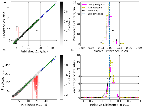
Figure 3: (a) Predicted value of $\Delta\nu$ at each value of published $\Delta\nu$ in all the detected stars by the neural network. The colour of each point in the plot denotes the confidence value of the prediction and the vertical red lines indicate 68% confidence interval. Published values are taken from Vrard et al. (2016).(b) Distribution of relative differences in $\Delta\nu$ in various regimes of real data (legends). The relative difference is calculated with respect to the published value ((predicted $\Delta\nu$-published $\Delta\nu$)/published $\Delta\nu$). The red-dashed line tracks zero difference. More than 90% of the predictions appear to lie well within 1.5% of the published values.(c) Predicted value of $\nu_{max}$ at each value of published $\nu_{max}$ on all the detected stars by the neural network. The colour of each point in the plot denotes the confidence value of the prediction and the vertical red lines indicate 68% confidence interval. Published values are taken from Yu et al. (2018); Chaplin et al. (2013).(d) Distribution of relative differences in $\nu_{max}$ in various regimes of real data (legends). The relative difference is calculated with respect to the published value ((predicted $\nu_{max}$-published $\nu_{max}$)/published $\nu_{max}$). The blue-dashed line tracks zero difference. More than 90% of the predictions appear to lie well within 5% of the published values. The green line in (a,c) tracks predicted parameter = published parameter. Points with blue open circles show the predictions of subgiant stars.

In Figure 3(c), $\nu_{max}$ predictions are plotted against the respective published $\nu_{max}$ values from Yu et al. (2018) and Chaplin et al. (2013). Figure 3(d) graph the distributions of relative differences between $\nu_{max}$ predictions and published values in young red giant branch, old red giant branch, and red clumps respectively. It indicates that $\nu_{max}$ is predicted well within 5% of the published values for 90% of stars. Therefore, these results along with $\Delta\nu$ predictions validate the neural network and also demonstrate that p modes are encoded correctly in the synthetic data set.

Figure 4: (a) Predicted value of $\Delta\Pi$ at each value of published $\Delta\Pi$ in all the detected stars by the neural network. The colour of each point in the plot denotes the confidence value of the prediction and the vertical red lines indicate 68% confidence interval. The green line tracks predicted $\Delta\Pi$ = published $\Delta\Pi$. Points with blue open circles show the predictions of subgiant stars. Published values are taken from Vrard et al. (2016); Mosser et al. (2014). (b) Distribution of relative differences in $\Delta\Pi$ in various regimes of real data (legends). The relative difference is calculated with respect to the published value ((predicted $\Delta\Pi$-published $\Delta\Pi$)/published $\Delta\Pi$). The blue-dashed line tracks zero difference. More than 90% of predictions appear to lie well within 5% of the published values.

Panel 4(a) capture $\Delta\Pi$ predictions against respective published $\Delta\Pi$ values in young red giant branch, old red giant branch, subgiants, and red clumps respectively. Panel 4(b) graph the distributions of relative differences between predicted and published $\Delta\Pi$ in each stellar class. The distributions of relative differences show that, for 90% of the stars, the neural network recovers $\Delta\Pi$ to within 7% of published values (Mosser et al., 2014; Vrard et al., 2016). These results also indicate that the machine works very well in predicting $\Delta\Pi$ in sub giants, young red giant branch and red clumps. Figure 4(d) shows that it is not quite as successful when applied to old red giants as well as to other evolutionary stages. In the old red-giant branch, 90% of the predictions are within 12% of the published results. This relatively poor performance may be ascribed to the lower mixed-mode coupling strengths for old red giants (Mosser et al., 2017), contributing to the comparatively diminished performance on synthetic data (Figure B.4) and the training data requiring a larger variety of templates.

In low-amplitude dipolar-mode stars e.g. (Mosser, B. et al., 2017), the neural network identifies these as solar-like due to the p-mode hump. Additionally, the network’s inference of $\Delta\Pi$ in these stars will not be reliable, as they are not modelled in the synthetic dataset.

Therefore, the method is highly accurate in young red giant branch, subgiants, and red clumps. In these stellar classes, 90% of the $\Delta\Pi$ predictions agree with published values to within 7%. This method is moderately accurate for the old red giant branch ($\Delta\nu<9\mu$Hz and $\Delta\Pi<150$s). In this stellar class, 90% of the $\Delta\Pi$ predictions agree with published values to within 12%. These results also prove that mixed modes are encoded correctly in the synthetic data set.

2.3 Evolution of stellar and core density in a red-giant

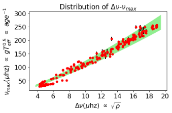
Figure 5: The distribution of $\Delta\nu$-$\nu_{max}$ for the stars listed in Tables C.1 and C.2. The red points correspond to ($\Delta\nu$, $\nu_{max}$) and the green band maps the relation given in Stello et al. (2009). The black lines associated with each point mark the 1-$\sigma$ interval. In most cases, the 1-$\sigma$ intervals are smaller than the sizes of the plotted points, and hence not visible to the naked eye. These parameters depend on stellar density ($\rho$) and age of the star. This plot indicates stellar density decreases as the star evolves.

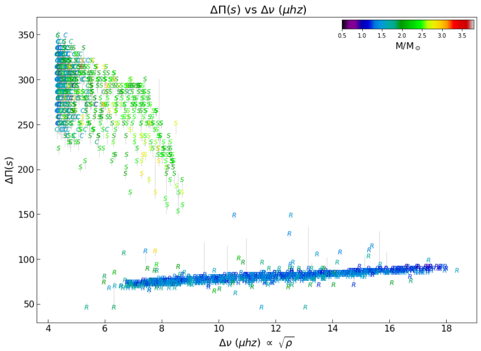
Figure 6: Machine $\Delta\Pi$ vs machine $\Delta\nu$ predictions. The colour of each point captures the ratios of stellar to solar masses (stellar masses are taken from Vrard et al. (2016)). The letters R,S,C represent red giants, secondary red clumps and red clump stars respectively. The grey lines demarcate 68% confidence intervals. All these predictions are highly confident. The plot indicates that there exists a nearly linear relationship between $\Delta\Pi$ and $\Delta\nu$ in red giants. $\Delta\nu$ depends on stellar density ($\rho$) of the star and $\Delta\Pi$ depends on core sizes of stars (Montalbán, J. & Noels, A., 2013). This plot indicates core size decreases as the stellar density decreases in red giants.

Figure 5 shows the $\Delta\nu$-$\nu_{max}$ distribution of stars given in Tables C.1 and C.2. It shows that most stars follow the relation given in Stello et al. (2009). However, at very low $\Delta\nu$, we note that several stars deviate by more than $1\sigma$ from the general trend, indicating a possible break of the scaling relation for most evolved stars. This deviation has also been observed for evolved stars in Huber et al. (2011), where they have observed a different $\Delta\nu-\nu_{max}$ relation for stars with $\nu_{max}<100\mu$Hz. This deviation is not an artifact of periodogram construction, as we have independently verified the predictions on periodograms from the lightkurve software (Lightkurve Collaboration et al., 2018). These parameters depend on stellar density ($\rho$) and age respectively (Kippenhahn et al., 2012). The plot shows that, as the star evolves, the stellar density decreases.

Figure 6 presents the $\Delta\Pi$-$\Delta\nu$ relation in red giants and red clumps. It shows that $\Delta\Pi$ and $\Delta\nu$ are approximately linearly related in red giants. $\Delta\Pi$ depends on the core size of the star (Montalbán, J. & Noels, A., 2013) and this plot shows that the core contracts as stellar density decreases with progressing stages of evolution. Even though this result is well established (Mosser et al., 2014), it is important for the following reasons:

• It serves as a validation test for the neural network and indicates high-quality synthetic data.

• The training data sets that were constructed do not have a built-in correlation between $\Delta\Pi$ and $\Delta\nu$. However, when applied to real data, the neural network finds a strong correlation between these two parameters ($\Delta\Pi$, $\Delta\nu$). This demonstrates that the machine is able to find the true correlation between these parameters in quick computational time.

2.4 Rare Systems

Figure 7: (a) Power spectrum of KIC 2997178. The red box in the power spectrum shows the red-giant component. The blue and green boxes in the plot highlights other two features of the power spectrum.(b) Power spectrum of the binary KIC 3338674 where the red-box in the power spectrum highlights the red-giant component.

As the four stellar classes given in the Table 1 have stellar oscillations in different frequency ranges, the trained networks survey different parts of the power spectrum. Therefore, this method can identify red giants in binaries as well. Table C.1 has four binary candidates KIC 2997178, KIC 3338674, KIC 2018906 and KIC 1295546, which are shown in Figures 7 and C.1. Figure 7(a) shows the power spectrum of KIC 2997178 highlighting three different parts of the power spectrum. The possible explanations for the three features of this power spectrum are:

• A red giant (marked in red) eclipsing another other star (marked in blue). The green box in this Figure 7(a) highlights the signal of this eclipse.

• An eclipsing binary candidate (green, blue) with a red giant in the background (red).

• A possible triplet which has a red giant.

3 Conclusion

We present an efficient machine-learning algorithm that learns the marginal distributions of global seismic parameters $\Delta\nu$, $\nu_{max}$, and $\Delta\Pi$. We create a library of synthetic data to train the machine and demonstrate its performance on oscillation spectra of stars in different stages of evolution. The network is calibrated and able to identify p- and mixed-mode patterns on synthetic data, since it accurately finds $\Delta\nu$, $\nu_{max}$, and $\Delta\Pi$.

The machine can successfully discern red giants from noise on Kepler data. In addition to the 17527 known stars that the machine has also identified, we have identified $\sim 25$ new red giants analysing 151,000 Kepler long-cadence stars in a few minutes of computation. We have provided the first period-spacing measurements of the $25$ new red giants and those of 195 red giants previously identified by Hon et al. (2019). Although not being trained explicitly to, the present method is still capable of detecting red giants in binaries. We have detected four new binaries with red-giant counterparts.

We validate the machine inferences using estimates from other methods by selecting $\sim$3,000 test stars from Mosser et al. (2014); Vrard et al. (2016), which are spread over a range of evolutionary stages. We observe that 90% of the predictions agree with published values to within 1.5% for $\Delta\nu$, 8% for $\Delta\Pi$ and 5% for $\nu_{max}$. Despite the training data containing no artificially introduced correlations among the seismic parameters, the machine has independently identified a linear relationship between $\Delta\Pi$ and $\Delta\nu$ in the observations, validating both the neural network and the synthetic spectra.

In future work, we will improve the machine learning model and synthetic data to improve estimates of $\Delta\Pi$, and expand the parameter space to include stars with $\Delta\nu<4.2\mu Hz$. We will investigate the undetected stars and special systems detected by the machine. We will optimize the training time of our machine learning model using multi-node setup. Also, the model will be expanded to infer all global seismic parameters, such as the coupling constant, core and envelope rotation rates, and inclination angle, by combining this method with Monte-Carlo-based techniques (Benomar et al., 2009; Handberg & Campante, 2011; Corsaro & De Ridder, 2014).

The neural network can study $\sim$1,000 stars in under $\sim$5 seconds, enabling ensemble asteroseismology on vast data sets. As the machine is completely trained on synthetic data, we can extend this to data from other missions with small changes (such as including mission-specific systematics) to the simulations. Future missions such as PLATO are expected to observe a million light curves, which might consist $>100,000$ solar-like stars. The network here can analyze and extract the physics of these stars within 10 minutes, and has the potential to transform asteroseismology.

Acknowledgment: S.D. acknowledges SERB, DST, Government of India, CII and Intel Technology India Pvt. Ltd. for the Prime minister’s fellowship and facilitating research. All the computations are performed on Intel^® Xeon^® Platinum 8280 CPU. We thank Dhiraj D. Kalamkar, Intel Technology India Pvt Ltd for the suggestions, which helped to optimize the neural network training. This paper includes data collected by the Kepler mission and obtained from the MAST data archive at the Space Telescope Science Institute (STScI). Funding for the Kepler mission is provided by the NASA Science Mission Directorate. STScI is operated by the Association of Universities for Research in Astronomy, Inc., under NASA contract NAS 5–26555. This research made use of Lightkurve, a Python package for Kepler and TESS data analysis (Lightkurve Collaboration, 2018). We thank Tim Bedding and the anonymous referee for providing constructive comments, which helped improve the quality of the paper.

Appendix A Methods and Techniques

A.1 Simulated spectra as a training data set

We build data sets using a simulator available at https://github.com/OthmanB/Spectra-Simulator-C that can generate synthetic spectra over a large range of parameters. The software incorporates the physics of structure, composition gradient, and rotation in red giants using the asymptotic theory of stellar oscillations García & Ballot (2019); Aerts et al. (2010). The simulator takes a random global seismic parameter set over a range specified by the user and generates a spectrum. For a specific set of parameters, different noise realisations are generated in order to train the machine to discriminate features from noise. In this section, we describe the asymptotic theory and preparation of synthetic data sets to train the machine

A.1.1 Frequencies of p and mixed modes

Global stellar oscillations are predominantly due to standing waves of two kinds, one where pressure is the restoring force (p modes) and the other where buoyancy is the restoring force (g modes). While p modes can travel all through the interior, pure g modes are trapped in the deep radiative zone and have surface amplitudes far too small to be observed. This is due to the fact that solar-like stars have a thick outer convective zone in which g-mode oscillations are evanescent. Ever since early theoretical work on this topic Unno et al. (1989), it is known that when the physical distance between the cavities of p modes and g modes become small enough or overlap, the modes may significantly interact to form so-called mixed modes. Unlike p modes that mostly probe outer convective layers, mixed modes provide a unique window into deep internal structure. Observational asteroseismology has revealed that prevalent conditions in red giants allow for the existence of mixed modes Bedding et al. (2010); Beck et al. (2011).

For unresolved disk photometry, degrees higher than $\ell>3$ modes cannot usually be observed due to geometrical cancellation effects that limit their apparent amplitude (see Section A.1.3).

In the case of a spherically symmetric, non-rotating star, $m$ components are degenerate and frequencies only depend on the degree and radial order. p-mode frequencies are then expected to approximately follow an asymptotic regime Tassoul (1980). In second-order asymptotic theory, the frequencies of p modes of radial order n and azimuthal order $\ell$ are given by Mosser et al. (2010, 2012)

$$\frac{\nu_{n,\ell}}{\Delta\nu}=n+\frac{\ell}{2}+\epsilon(\Delta\nu)-d_{0\ell}(\Delta\nu)+\frac{\alpha_{\ell}}{2}\left(n-\frac{\nu_{max}}{\Delta\nu}\right)^{2},$$ (A1)

where $\Delta\nu$ is the large-frequency separation, which gives the mean-frequency separation between two successive radial modes, $\epsilon(\Delta\nu)$ is the offset parameter, $d_{0\ell}$ the small-frequency separation, and $\alpha_{\ell}$ the degree-dependent gradient $\alpha_{\ell}=\left(d\log\Delta\nu/dn\right)_{\ell}$.

The term $\nu_{max}$ in Equation A1 refers to the frequency corresponding to maximum amplitude. Observations Stello et al. (2009) and scaling relations Ulrich (1986) have demonstrated a strong interdependent relation between $\Delta\nu$ and $\nu_{max}$. For our simulations, we choose $\nu_{max}$ based on $\Delta\nu$ from the relation given in Stello et al. (2009), with 10% deviation, as follows

$$\nu_{max}=(\Delta\nu/0.263)^{1/0.772}\pm 0.1(\Delta\nu/0.263)^{1/0.772}.$$ (A2)

For solar-like stars, mixed modes start to become visible in the power spectra when a star reaches the end of the main-sequence. There is an increase in the density gradient in the core, which causes the Brunt-Väisälä frequency ($N$) to rise. As illustrated in Figure A.1, one consequence is that the acoustic and buoyancy cavities become closer to each other. As a result, the coupling between the interior g modes and p modes grows stronger. The strength of coupling is indirectly proportional to the physical distance between these cavities Mosser et al. (2017). Mixed modes exhibit characteristics of both types of oscillations at the same eigenfrequency. This mode is oscillatory in the radiative core and the acoustic envelope but evanescent in the region that connects the cavities.

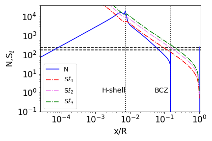
Figure A.1: Wave propagation diagram in a 1.3M_⊙ star at 4.51 Gyr, in a young red-giant phase

; plotted are Lamb and Brunt-Väisälä frequencies as a function of the fractional radius. Lamb frequencies determine the p-mode cavities of the respective $\ell$ modes and Brunt-Väisälä frequencies set the g-mode cavity. The horizontal dashed lines denote the ranges of observable frequencies for this red-giant star. The vertical dotted lines demarcate the Hydrogen shell and base of convection zone.

Largely, the observed mixed modes are dipole modes as dipole p modes travel deeper into the star and hence have higher coupling strength with dipole g modes compared to $\ell=2,3$ modes. Figure A.1 shows that dipole p-mode cavity probe deeper than $\ell=2$ and $\ell=3$ p mode cavities. Even though there are observed cases of $\ell=2$ mixed modes Benomar et al. (2013), they are exceptions and have very low coupling strength. Therefore, in our simulation, we consider $\ell=2$ and $\ell=3$ as pure p modes and dipole modes as mixed modes. The coupling phenomena between p and g modes was theorised by Unno et al. (1989) and formally expressed in the case of evolved solar-like stars using asymptotic relations for p and g modes by Mosser et al. (2012). They derived the following implicit equation that gives the solutions of dipole mixed-mode frequencies,

$$\tan\pi\frac{\nu-\nu_{p}}{\Delta\nu}=q\tan\frac{\pi}{\Delta\Pi}\left(\frac{1}{\nu}-\frac{1}{\nu_{g}}\right),\hskip 5.69046pt$$ (A3)

where $q$ is the coupling factor between p and g modes, $\nu_{p}$ is the frequency of a pure p mode, $\nu_{g}$ is the frequency of a g mode, and $\Delta\Pi$ is the period spacing that depends on the integral of the Brunt-Väisälä frequency and is therefore sensitive to the deep interior structure of solar-like stars. It defines the period separation between successive pure g modes, asymptotically regularly spaced in period,

$$\frac{1}{\nu_{g}}=\left(-n_{g}+\epsilon_{g}\right)\Delta\Pi$$ (A4)

where $n_{g}<0$ is the radial order of the pure g mode and $\epsilon_{g}$ is the offset parameter. When solving equation A3, the second-order asymptotic relation shown in equation (A1) is used for p-mode frequencies as well as the equation A4 for the g modes frequencies.

Due to the difference in gradients of the Brunt-Väisälä and Lamb frequencies, the coupling factor is expected to vary. However, in the simulations, it is assumed that these variations remain small within the range of observed frequencies so that $q$ is set to be constant. This commonly invoked assumption has been shown to be accurate in past studies Mosser et al. (2015).

A.1.2 Effect of Rotation

Evolved solar-like stars are known to show significant radial differential rotation Deheuvels et al. (2014). The core-to-envelope rotation contrast can range up to a few tens, and its imprint on the pulsation frequencies must be taken into account in realistic simulations.

While the asymptotic relations described in Section A.1.1 remain valid, rotation breaks the spherical symmetry of the star and lifts the degeneracy in $m$. The Sun shows radial and latitudinal differential rotation (e.g., Schou et al., 1998), with a mean sidereal rotation rate of $\sim$435 nHz (the $a_{1}$ coefficient). Slow rotation, as in the Sun, may be treated as a small perturbation to the non-rotating case. Each mode of degree $\ell$ splits into $2\ell+1$ azimuthal components, with $m\in[-\ell,\ell]$. The mode $\nu_{n,\ell,m}$ is given by $\nu_{n,\ell,m}=\nu_{n,\ell}+\delta\nu_{n,\ell,m}$, with $\delta\nu_{n,\ell,m}$ being the rotational splitting. Considering that the radial differential rotation dominates relative to latitudinal differential rotation, it may be expressed as a weighted average of the rotational profile,

$$\delta\nu_{n,\ell,m}=m\int^{R}_{0}K_{n,l}(r)\Omega(r)dr,$$ (A5)

where $K_{n,l}$ is the rotation kernel, defining the sensitivity of the modes as a function of radial position $r\in[0,R]$ within the star.

Because p modes are mostly sensitive to average rotation within the stellar interior Benomar et al. (2015), the dependence of $\delta\nu_{n,\ell,m}$ on $(n,\ell)$ is weak within the observed frequency range of a solar-like star Lund et al. (2014). In fact, it does not exceed a few percent even in the presence of radial differential rotation of a factor two between the convective zone and the radiative zone. Note that in the Sun, this differential rotation is of $\simeq 30\%$, while on other solar-like stars, it is below a factor two Benomar et al. (2015); [Nielsen et al. (2017). Such upper limit factor leads to splitting variations of the same other as that achieved in the 1$\sigma$ uncertainties of the best seismic observations from Kepler. It is accurate to express the rotational splitting of p modes as

$$\nu_{n,\ell,m}=\nu_{n,\ell}-m\nu_{s},$$ (A6)

where $\nu_{s}=\Omega/2\pi$ is the integral term of equation A6, a function only of the average internal rotation $\Omega$ rate. The rotational kernels of p modes are highly sensitive to outer layers of stars. In main-sequence stars, approximately $60\%$ of the average rotation rate $\Omega$ comes from the contribution of the envelope rotation. For red giants, which have a much larger envelope than main-sequence stars, this contribution exceeds $80\%$, e.g., Figure A.1. And it is common to consider that $\nu_{s}$ essentially measures the rotation in the envelope, so that $\nu_{s}\simeq\Omega_{env}/2\pi$ (Goupil, M. J. et al., 2013).

The $\ell=1$ modes and $\ell=2,3$ modes are affected differently by the rotation in red giants. $\ell=2,3$ modes are considered to be pure p modes so that frequencies of split components are considered to follow equation A6.

The mixed modes are primarily present in the $\ell=1$ oscillations and these are influenced by both the core (g modes) and the envelope (p modes). Due to the mode mixing, Kernels $K_{n,\ell=1}(r)$ differ significantly from one mode to another. Some mixed modes indeed are weakly sensitive to the core while others show strong sensitivity. However, Goupil et al. (2013) has shown that a two-zone model of rotation can well account for $\ell=1$ splittings observed in red giants and early subgiants. Under that assumption, they also demonstrated that rotational splitting is a linear function of the ratio between the kinetic energy of modes in the g modes cavity and the total kinetic energy of modes, denoted $\zeta(\nu)$,

$$\mathrm{\delta\nu_{rot}}=-\frac{1}{2}\frac{\Omega_{core}}{2\pi}\zeta(\nu)+\frac{\Omega_{env}}{2\pi}(1-\zeta(\nu)).$$ (A7)

Furthermore, it was found Deheuvels et al. (2015) that the $\zeta(\nu)$ function is well approximated by,

$$\zeta(\nu)=\left[1+\frac{1}{q}\frac{\nu^{2}\Delta\Pi}{q\hskip 1.42271pt\Delta\nu}\frac{\cos^{2}\pi\frac{1}{\Delta\Pi}\left(\frac{1}{\nu}-\frac{1}{\nu_{g}}\right)}{\cos^{2}\pi\frac{\nu-\nu_{p}}{\Delta\nu}}\right]^{-1},$$ (A8)

which is defined by the same quantities as equation A3. When $\zeta(\nu)$ is close to one, the mode is mainly trapped in the g-mode cavity (and thus is more sensitive to the stellar core). A value of $\zeta(\nu)$ close to 0 correspond to a mode essentially trapped in the p-mode cavity.

This expression is broadly used to determine the rotational splittings of red giants by various authors such as Mosser et al. (2018), but it is a crucial relation that also describes the observed period spacing (Gehan et al., 2018), the amplitudes and the width variations as functions of the mode frequency in evolved stars (see Section A.1.3).

A.1.3 Relative heights and widths of different modes

Figure A.2: This figure demonstrates the conversion of the observed spectral template (KIC 12508433) into a synthetic spectral template. (a) Amplitude and width profiles of KIC 12508433. (b) Amplitude and width profiles of a synthetic star ($\Delta\nu=12\mu$Hz, $\Delta\Pi=80$s, $q=0.1$, $\Omega_{core}/2\pi=1\mu$Hz, $\Omega_{env}/2\pi=0.05\mu$Hz, $\iota=54.4^{\circ}$) that is based on the template of KIC 12508433. The solid (dashed) lines in both figures correspond to $\ell=0$ ($\ell=1$) modes. The blue (red) lines in both figures correspond to amplitude (width) profiles.

Each mode in the power spectrum is modeled using a Lorentzian function centered around frequency $\nu(n,\ell,m)$ with height $H(n,\ell,m)$ and width $\Gamma(n,\ell,m)$. The linewidths $\Gamma(n,\ell)$ of p modes in the power spectrum increase with frequency (Appourchaux et al., 2014). The excitation and damping of modes is not well understood, mostly due to non-adiabatic effects near the stellar surface, which are difficult to model. Yet our simulations need to have realistic mode heights and widths. To circumvent this issue, we use templates obtained by fitting real stars and rescale them following an adapted version of the method from Kamiaka et al. (2018). In this technique, the heights, widths and average splittings of p modes are rescaled. For l=0,2,3 p modes, the procedure here is similar. However because individual pulsation frequencies of the template are different than those of the simulated star (and given by equation A1), it is important to correct for differences in $\nu_{max}$ and $\Delta\nu$. Linear interpolation is performed to stretch and recenter the template height and width at the frequencies of the simulated star. This allows us to obtain profiles for $\ell=0,2,3$ p modes that are identical to that of the template but recentered at the $\nu_{max}$ of the simulated star.

As revealed by Benomar et al. (2013); Grosjean et al. (2015), mixed modes show complex amplitude and width variations with frequency. Motivated by this observational evidence, Benomar et al. (2014) found that the mode inertia ratios between $\ell=1$ and $\ell=0$ modes are expressed as

$$\frac{I_{1}}{I_{0}}=\sqrt{\frac{A_{0}}{A_{1}}}\frac{\Gamma_{0}}{\Gamma_{1}},$$ (A9)

where $A_{0}\propto\sqrt{\pi H_{0}\Gamma_{0}}$, $A_{1}\propto\sqrt{\pi H_{1}\Gamma_{1}}$ denotes the amplitudes of $\ell=0$ and $\ell=1$ modes and $\Gamma_{0}$, $\Gamma_{1}$ are the mode widths. Grosjean Mathieu (2015) found that, under the assumption of equipartition of energy between modes, and accounting for damping and excitation assuming no radiative pressure, the product of inertia and width is conserved between $\ell=0$ and $\ell=1$ modes,

$$I_{1}\Gamma_{1}=I_{0}\Gamma_{0}.$$ (A10)

Furthermore, Mosser et al. (2015) found that the inertia ratio may be expressed as a function of $\zeta(\nu)$,

$$\frac{I_{1}}{I_{0}}=\frac{1}{1-\zeta(\nu)}.$$ (A11)

Equations A9, A10, A11 may be used to derive the amplitudes and widths of the mixed modes,

$$\Gamma_{1}(\nu)=\Gamma_{0}(1-\zeta(\nu));\hskip 5.69046ptA_{1}^{2}(\nu)=A_{0}^{2}(1-\zeta(\nu)).$$ (A12)

Due to the assumptions made for reaching this expression, it may be accurate only for less evolved stars, i.e., red giants and subgiants. However, as shown in Section 2, it remains accurate enough for red clump stars as well, ensuring that the current machine-learning approach does not introduce biased results on fundamental quantities defining the mixed-mode frequencies.

Figure A.2 illustrates an example of this procedure of producing a template for synthetic star. It exhibits an amplitude and width profile of KIC 12508433, and shows a template prepared for the synthetic star. The blue (red) solid lines represent amplitude (width) of the $\ell=0$ modes. It can be observed that amplitudes of $\ell=0$ modes are nearly symmetric with respect to $\nu_{max}$ in both cases. Also, the amplitudes and widths of the template follow the same trend as the original star, establishing the method of conversion described in this subsection.

A.1.4 Effect of mode visibility and of stellar inclination

When observing oscillations of distant stars at low spatial resolution, the visibility of mode $f_{n,\ell,m}=AY_{\ell}^{m}(\theta,\phi)$ is given by

$$a_{n,\ell,m}=r_{\ell,m}(\iota)V(\ell)A,$$ (A13)

where $V(\ell)$ is the mode visibility, $r_{\ell,m}(\iota)$ the relative amplitude of the mode, which depends on the inclination angle $\iota$. The visibility function depends on the limb-darkening function (star type) and the measurement technique used.

The visibility function $V(\ell)$ decreases with increasing degree $\ell$. Therefore, we dominantly observe only $\ell=0,1$ and $2$ modes in the asteroseismic data, as the amplitude decreases for other degree modes; the $\ell=1$ mode has higher visibility than $\ell=0$. We rarely observe $\ell=3$ modes. From studies on various red giants Mosser et al. (2012a), it is assumed that $V(0)\simeq 1$, $V(1)\in[1.2,1.75]$, $V(2)\in[0.2,0.8]$ and $V(3)\in[0,0.1]$.

The relative amplitude is given by the following equation:

$$r_{\ell,m}^{2}\left(\iota\right)=\frac{(\ell-|m|)!}{(\ell+|m|)!}\left[P_{\ell}^{|m|}(\cos\iota)\right]^{2},$$ (A14)

where $P_{\ell}^{|m|}$ is the associated Legendre polynomial. To maintain an isotropic distribution of stellar-axis inclinations, the prior for the angle is taken to be $P(\iota)\propto\sin(\iota)$.

A.1.5 Noise Model

The background noise model comprises a combination of white noise and a Harvey-like profile. At high frequencies, noise is dominated by white noise (photon noise), which is independent of frequency. At low frequencies, noise is generated by surface convection (granulation), described by the Harvey profile Harvey (1985). While there are models considering additional facular signatures Karoff et al. (2013), these are not the dominant features Karoff (2012) and hence are ignored here. Equation A15 contains the background noise model $B(\nu)$:

$$B(\nu)=\frac{H}{1+(\tau\nu)^{p}}+N_{0},$$ (A15)

where H is the characteristic granulation amplitude, $\tau$ is the characteristic timescale of granulation, $p$ is the characteristic power law, and $N_{0}$ is the white noise level.

It has been observed that the granulation amplitude and timescale vary with $\nu_{max}$ Kallinger & Matthews (2010); Mathur et al. (2011); Chaplin et al. (2011). Considering this, we model the granulation amplitude and timescale as

$$H=A_{g}\nu_{max}^{B_{g}}+C_{g},\,\,\,\,\,\tau=A_{\tau}\nu_{max}^{B_{\tau}}+C_{\tau},$$ (A16)

where the triplet ($A_{g},B_{g},C_{g}$) has free parameters that modify granulation amplitude and ($A_{\tau},B_{\tau},C_{\tau}$) modify the granulation timescale. We have created a wide variety of noise profiles by taking a range of values for these parameters, as given in Table 1.

A.1.6 Description of the Data sets

We generate 3 million random synthetic stellar spectra spanning the range of seismic parameters described in Table 1. The spectra in the data set possess a variety of different features apart from the primary set of seismic parameters: (a) variable number of peaks, (b) various height profiles, (c) variable resolution and (d) uniform prior in parameter space.

In step (a), stellar spectra in the data set have different numbers of modes since real data show differing numbers of peaks. This step is important as parameter prediction must be robust to changes in the magnitude of the star and signal-to-noise ratio. As the magnitude of the star and SNR rise, the number of observed peaks increases.

For step (b), we generate the data set based on nine amplitude profiles of different stars. Each spectrum randomly selects an amplitude profile among these stars and creates a template according to the method described in Section A.1.3. As our parameter set is a function of the peak positions, this step ensures that parameter prediction is independent of height. To create this data set, we have selected the following profiles: KIC 10147635, KIC 11414712, KIC 12508433, KIC 6144777, KIC 8026226, KIC 11026764, KIC 11771760, KIC 2437976, KIC 6370489.

In step (c), we generate half the stellar spectra in the data set with frequency resolution of 4 yrs and the remainder for 3 yrs. When we select samples for training, we linearly interpolate spectra with lower resolution to a higher resolution. This step is crucial, as real data show fluctuations in frequency resolution.

In the final step (d), we avoid class imbalance by drawing all the samples from a uniform prior in parameter space (except inclination angle). The inclination angles are drawn from a uniform distribution in $\sin\iota$. To avoid bias in the parameter prediction, we actively reject correlations among different seismic parameters.

Table A.1: Parameter space in different evolutionary stages of giant stars.

Parameter	Subgiant	Young red giant branch	Old red giant branch	Red clumps	Red giant simulations
Range of $\Delta\nu$	18-50 $\mu$Hz	9-18 $\mu$Hz	6-9 $\mu$Hz	4.2-12 $\mu$Hz	1-18.7 $\mu$Hz
Range of $\Delta\Pi$	60-200s	45-150s	45-110s	150-500s	45-500s
Range of q	0.05-0.5	0.05-0.5	0.05-0.5	0.05-0.75	0-0.75
Range of $\epsilon_{p}$	0-1	0-1	0-1	0-1	0-1.
Range of $\epsilon_{g}$	0-1	0-1	0-1	0-1	0-1.
Range of $d_{0\ell}$	0.005-0.025	0.005-0.025	0.005-0.025	0.005-0.025	0.005-0.025
Range of Core	0.005-4.0	0.005-4.0	0.05-3.0	0.005-1.0	0.005-1.0
rotation ( in $\mu$Hz)
Range of Envelope	0.005-0.4	0.005-0.4	0.005-0.4	0.005-0.4	0.005-0.4
rotation ( in $\mu$Hz)
Range of $\iota$ ( in deg)	0-90	0-90	0-90	0-90	0-90
Range of $A_{g}$	0.8-1.2	0.8-1.2	0.8-1.2	0.8-1.2	0.8-1.2
Range of $B_{g}$	-2.2 - -1.8	-2.2 - -1.8	-2.2 - -1.8	-2.2 - -1.8	-2.2 - -1.8
Range of $C_{g}$	0-0.5	0-0.5	0-0.5	0-0.5	0-0.5
Range of $A_{\tau}$	0.8-1.2	0.8-1.2	0.8-1.2	0.8-1.2	0.8-1.2
Range of $B_{\tau}$	-1.2 - -0.8	-1.2 - -0.8	-1.2 - -0.8	-1.2 - -0.8	-1.2 - -0.8
Range of $C_{\tau}$	0-0.5	0-0.5	0-0.5	0-0.5	0-0.5
Range of $p$	1.8-2.2	1.8-2.2	1.8-2.2	1.8-2.2	1.8-2.2
Range of $N_{0}$	0.1-0.4	0.1-0.4	0.1-0.4	0.1-0.4	0.001-40,000
Frequency range used	250-1150$\mu$Hz	60-262 $\mu$Hz	22-192 $\mu$Hz	22-192 $\mu$Hz	0-250$\mu$Hz
for ML training
Range of Observation	1065-1460 days	1065-1460 days	1065-1460 days	1065-1460 days	9-1460 days
time
SNR distribution	5-70	5-70	5-70	5-70	5-150

Note. — First four column show the parameter space in different evolutionary stages of giant stars.This table shows the range of parameters that were chosen to create different synthetic data sets. This range of parameters is chosen so as to cover the space of published results on Kepler Data Mosser et al. (2015); Vrard et al. (2016); Mosser et al. (2017). Last column shows the parameter space used to produce the red-giant and pure noise simulations. The noise simulations are produced with a 0 signal to noise ratio (SNR).

A.2 Machine Learning Model

Machine learning methods have a common algorithmic approach, namely to train a machine to carry out a task using a training data set. Here, we use a deep neural network, detailed hereafter for the purpose of power spectral analysis.

We want the machine to recognize the non-linear relationship between the normalized spectral data X and the (seismic) parameters Y (in Table 1) using deep neural networks $f$, i.e.,

$$f(\mathrm{X;W})\approx\mathrm{Y},$$ (A17)

where rows of X are examples presented to the machine to learn about the parameters, W represents the neural network parameters, and Y is the dependent variable (seismic parameter). Each row of X is a normalized power spectrum. It is obtained by dividing the power spectrum by the maximum power in the used frequency range. X and Y have same number of rows. Rather than predicting real-valued seismic parameters, we first pose a classification problem by categorizing the seismic parameter space using uniformly-spaced bins. This turns each row of Y into a one-hot encoded vector. In one-hot encoding, all the elements of the vector are 0 except the ground truth, which is represented by 1. In this case, the number of columns of Y is the number of bins and a 1 is associated with the ground truth. For example, let a seismic parameter $\theta$ be in range 0 to 50 and the number of bins be 5. Let $i$-th data be generated by a seismic parameter $\theta_{i}$ of value 37. Then, this target $\theta_{i}$ is encoded as [0,0,0,1,0] in the corresponding row of Y. Also, each bin in this method is represented by its mean value (i.e., 5, 15, 25, 35, and 45, respectively, in this example) and a predicted parameter takes only one of these mean values.

For a given normalized spectrum as input, the network outputs a vector of classification scores for the bins. We then apply a so-called softmax function (Bishop, 2006; Ian et al., 2016) to convert these scores to probability values and finally apply categorical cross-entropy loss (Murphy, 2013; Ian et al., 2016) on the output probability. We employ the ADAM optimizer (Kingma & Ba, 2017) for back propagation. Back propagation trains the neural network by adjusting its parameters W such that they minimise the loss function through a feedback loop between the outputs and the inputs. After completing the training, the network learns the approximate marginal probability distribution of the corresponding seismic parameter. As input, the bin with highest probability ($p_{max}$) is the best-fit seismic parameter whose value is the mean over that bin. We term $p_{max}$ as “confidence” since it is the confidence score of the predicted seismic parameter.

The choice of bin size is an important factor in this method. For larger bin sizes, a single representative value fails to capture the larger variety of data and consequently, parameter sensitivity is lost in the prediction. On the other hand, smaller bin sizes indicate superior resolution in parameter space. However, this results in a much larger classification problem that requires enormous amounts of data that well-represent each class. In other words, with limited data, such predictions become unreliable.

Figure A.3 shows the detailed architecture of the machine learning network, which is built by these layers. The core network comprises six convolutional layers (conv1D), followed by two long short term memory (LSTM) cells, and one dense layer. This network takes an input normalized power spectrum of length and outputs the probability associated with each bin of seismic parameter.

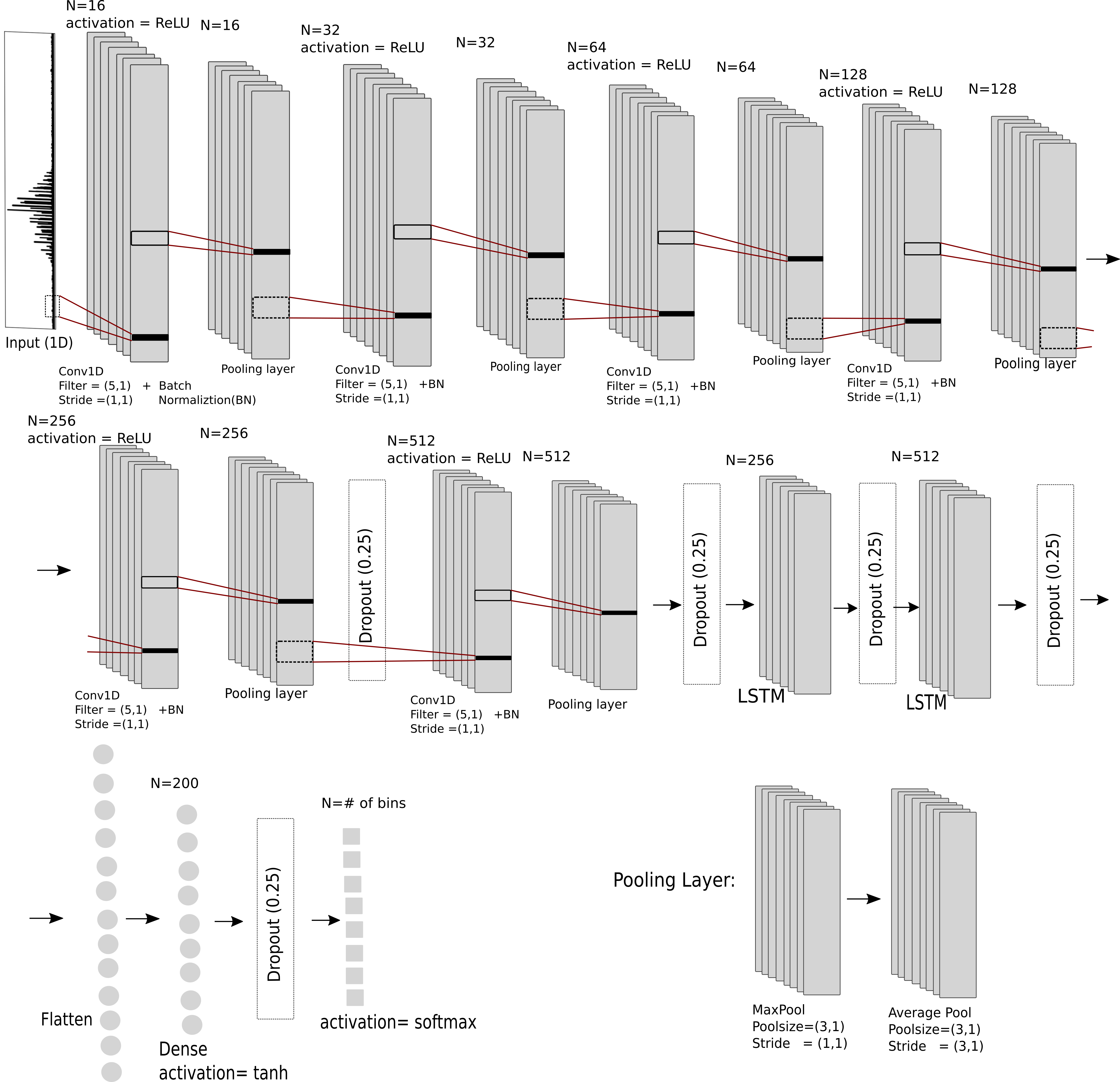
Figure A.3: Detailed architecture of neural network used in our machine learning algorithm. The core network consists of 6 CNN layers, 2 LSTM cells and a dense layer. In addition to them, 5 dropout layers with a fraction of 0.25 are used to prevent overfitting. right-bottom: This figure describes the components of Pooling layer. This network takes as input the (1D) normalized spectrum and outputs an approximate probability distribution of the subject parameter.

Computational time: This network has been trained on a single Intel^® Xeon^® Platinum 8280 CPU with 56 cores using tensorflow, a python based software used for machine learning (Abadi et al., 2015). The training took $\sim$ 50 node hours for each seismic parameter. For three seismic parameters in four different regimes, we train a separate network with identical architecture. The computational cost for training these 12 networks is 600 node hours (50 node hours each). The trained machine takes $\sim$5 milliseconds of computational time on a single core to predict one parameter on a star. In comparison, estimation of (i) $\Delta\nu$ takes $\mathcal{O}$(min)/star using auto-correlation method (ii) $\nu_{max}$ takes $\mathcal{O}$(min)/star by fitting a gaussian-envelope (iii) $\Delta\Pi$ takes $\mathcal{O}$(hr)/star using MCMC.

Appendix B Results on Synthetic data

Figure B.1: Probability distribution of the period-spacing $\Delta\Pi$ for three different synthetic young red giant branch. The true value that generates the spectrum is indicated by the black dashed line. The majority($>$95%) of the probability distributions are of type (a) and 5% of the distributions include types (b) and (c).

Table B.1: Choice of $\Delta\nu$, $\nu_{max}$ and $\Delta\Pi$ resolution for different stellar classes.

Stellar class	$\Delta\nu$ bins ($\mu$Hz)	$\nu_{max}$ bins ($\mu$Hz)	$\Delta\Pi$ bins (s)
Subgiants	[18,18,2],[18.2,18.4],	[229.88,233.89],$\dots$	[60,62.8],$\dots$,
	$\dots$,[48.8,50]	[952.30,956.31]	[197.2,200]
Young red giant branch	[9,9.2],[9.2,9.4],	[93.49,95.47],$\dots$,	[45,47.28],$\dots$,
	$\dots$,[17.8,18]	[251.95,253.93]	[147.72,150]
Old red giant branch	[6.0,6.1],[6.1,6.2]	[55.18,57.18],$\dots$,	[45,47.16],$\dots$,
	$\dots$,[8.9,9]	[102.18,104.18]	[107.84,110]
Red clump stars	[4.2,4,3],[4.3,4.4],	[34.75,36.73],$\dots$,	[150,157],$\dots$,
	$\dots$,[11.9,12]	[147.99,149.97]	[493,500]

For each stellar class given in Table 1, we train the machine separately, leaving four different machines for each parameter, where the core networks (CNN-LSTM-dense) are identical but the final layers change in accordance with the parameter and resolution required. Choices for the bins and parameter resolution in each evolutionary regime are given in Table B.1.

Once trained, the neural network’s performance is evaluated on a test data set, which comprises the unseen data. For the preparation of the test data set, we generate 120,000 synthetic stars in various evolutionary stages. The test and training data sets follow the same distribution in parameter space, as described in Table 1. We present the results of $\Delta\nu$, $\nu_{max}$, and $\Delta\Pi$ predictions on this data set.

For every input of a synthetic star’s normalized power spectrum, the output of the network is the probability in each bin, from which we construct the approximate probability distribution. These distributions take on varied forms, as demonstrated in Figure B.1.

Figure B.1 shows the probability distributions of $\Delta\Pi$ in three different stars. For the probability distribution shown in Figure B.1(a), the true value which generated the synthetic spectrum matches the neural network prediction with a confidence ($p_{max}$) of 0.6 approximately. More than 95% of the probability distributions are of the type B.1(a) but in the remaining $\sim 5\%$ of other cases, we encounter distributions of types B.1(b) and B.1(c). For the multimodal distribution shown in the Figure B.1(b), the true value matches the second peak of the distribution, whereas the distribution in Figure B.1(c) is flat. The machine is successful in its first prediction whereas it fails in two other cases. Although the machine is unsuccessful in the second case (Fig. B.1(b)), it is possible to test if any of the peaks in the distribution fit the spectrum using forward calculations. Obtaining a rapid estimate of the distribution is valuable since, despite the low confidence results, these could still serve as priors for methods such as Bayesian inference.

Figure B.2: Summary of results of $\Delta\nu$ predictions on synthetic data. (a) Relative prediction error in different regimes of synthetic data (legends). The relative error is calculated in reference to the true value that generates the spectrum. The blue-dashed line marks the zero-error. This shows that predictions lie within 1% of the true values. (b) Predicted values of $\Delta\nu$ at each value of true $\Delta\nu$ for all 120,000 synthetic red giants ($\Delta\nu$:4.2-50$\mu$Hz), across all stellar classes. The color of each point in the plot represents prediction confidence. The green line shows Predicted $\Delta\nu$ = True $\Delta\nu$. These figures show that $\Delta\nu$ can be inferred within 1.5% of the ground truth for 99.9% of stars.

Figure B.3: Summary of results of $\nu_{max}$ predictions on synthetic data.(a) Relative prediction error in different regimes of synthetic data (legends). Relative error is calculated in reference to the true value that generates the spectrum. The blue-dashed line marks the zero-error. This shows that predictions lie within 2.5% of true values. (b) Predicted value of $\nu_{max}$ at each value of true $\nu_{max}$ for all 120,000 synthetic red giants, across all stellar classes. The colour of each point in the plot represents prediction confidence. The green line shows Predicted $\nu_{max}$ = True $\nu_{max}$. These figures show that $\nu_{max}$ can be inferred within 3% of the ground truth for 99.9% of stars.

Figure B.4: Summary of results of $\Delta\Pi$ predictions on synthetic data. (a) Relative prediction error in different regimes of synthetic data (legends). Relative error is calculated in reference to the true value that generates the spectrum. The blue-dashed line marks the zero-error. This shows that predictions lie within 4% of true values. (b) Predicted value of $\Delta\Pi$ at each value of true $\Delta\Pi$ for all 120,000 synthetic red giants, across all stellar classes. The color of each point in the plot represents prediction confidence. The green line shows Predicted $\Delta\Pi$ = True $\Delta\Pi$. These figures show that $\Delta\Pi$ can be inferred within 4% of the ground truth for 99.5% of stars.

As in Figure B.1, we infer $\Delta\nu$, $\nu_{max}$, and $\Delta\Pi$ from an ensemble of 30,000 synthetic stars in each stellar class of Table 1. We present these results in Figures B.2,  B.3, and B.4.

Figure B.2(a) demonstrates that the machine is able to recover $\Delta\nu$ to within 1% of the original $\Delta\nu$. Figure B.2(b) shows the variation of predictions with true values of $\Delta\nu$. It indicates that predictions and true values are highly correlated. Therefore, these figures prove that the machine can identify $p$-mode patterns in synthetic data and predict $\Delta\nu$ accurately.

Figure B.3(a) shows that the machine is able to recover $\nu_{max}$ to within 2.5% of the true $\nu_{max}$. Figure B.3(b) graphs the variation of predictions with true values of $\nu_{max}$. It demonstrates that predictions and the true values are highly correlated. Therefore, these figures prove that the machine can predict $\nu_{max}$ accurately on synthetic stars.

Figure B.4(a) shows that the machine is able to recover $\Delta\Pi$ to within 2.5%. It also indicates that the machine performs relatively poorly on old red giant branch, where the error is 4%, compared to the error of $<3\%$ on the other stellar classes. Figure B.4(b) shows the variation of predictions with the true value of $\Delta\Pi$ that generates the power spectrum. It demonstrates that predictions and true values are highly correlated and that the correlation increases with confidence in predictions. Therefore, these results indicate that the machine can identify mixed mode pattern in synthetic data and infer $\Delta\Pi$ accurately.

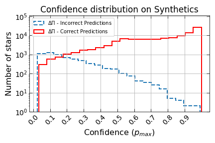
Figure B.5: This plot shows the distribution of confidence in $\Delta\Pi$ predictions. It shows the histograms of confidence in Correct predictions (Predictions of $\Delta\Pi$ within $<=$5% of ground truth) and Incorrect predictions (Predictions of $\Delta\Pi$ exceeding $>$5% of ground truth) on an ensemble of 120,000 synthetic stars, across all the stellar classes. The red (blue-dashed) histogram is the confidence distribution in Correct predictions (Incorrect predictions) predictions. Accuracy is seen to increase with growing confidence.

Figure B.1 shows predictions with three different confidence ($p_{max}$) values. We highlight the importance of confidence in Figure B.5, which plots the confidence distributions in correct and incorrect predictions of $\Delta\Pi$ with reference to true values. If the relative error is less than 5%, predictions are considered correct and otherwise, incorrect. Figure B.5 suggests that predictions with higher confidence ($p_{max}$) are more likely to be correct. Therefore, confidence acts as an indicator of the accuracy of prediction. In the following subsection, we also show that confidence ($p_{max}$) values produced by the machine are calibrated and represent true likelihood of the prediction.

B.1 Calibration test of the Network

We define two goals for this network: to be accurate and to provide the right estimate of the likelihood. In other words, the confidence estimates provided by the network have to return the correct likelihood/probability. Therefore, the network needs to be calibrated, for which we perform the following test Guo et al. (2017).

Consider that the machine returns a value $\hat{Y}$ with confidence $\hat{P}$. If the network is calibrated, it returns the true probability. Therefore,

$$\mathbf{P}(\hat{Y}=Y|\hat{P}=p)=p.$$ (B1)

Suppose we have $N$ predictions at confidence of $p$: the expected number of accurate predictions is therefore $Np$. The prediction is deemed accurate if the neural network finds the bin corresponding to the ground truth. In this calibration test, we compare the fraction of accurate predictions with confidence values in the range ($p$-$\epsilon$, $p$+$\epsilon$) to confidence $p$ and expect them to be identical.

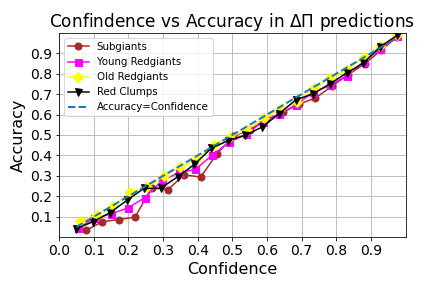
Figure B.6: Accuracy as a function of confidence in different regimes of synthetic data (legends). The blue dashes track the Accuracy = Confidence line. This shows that accuracy is approximately equal to confidence at each confidence level in different regimes, which agrees with the calibration test.

The results of the calibration test are presented in Figure B.6. The accuracy, shown for the range of confidence values in each stellar class, is approximately equal to confidence at every confidence level and every evolutionary stage. We interpret this result as indicating that the machine has passed the test in all evolutionary stages of giant stars and provides meaningful likelihood values.

Appendix C

Figure C.1: (a) Power spectrum of the binary KIC 1295546 where the red-box in the power spectrum highlights the red-giant counterpart. (b) Power spectrum of the binary KIC 2018906 where the red-box in the power spectrum highlights the red-giant counterpart.

Table C.1: This table shows the list of new giant stars that are discovered by Machine. It lists the measurements of $\Delta\nu$, $\nu_{max}$ and $\Delta\Pi$.

	KIC ID	$\Delta\nu$	Error	$\Delta\Pi$	Error	$\nu_{max}$	Error
		($\mu$Hz)	in $\Delta\nu$ ($\mu$Hz)	(s)	in $\Delta\Pi$	($\mu$Hz)	in $\nu_{max}$ ($\mu$Hz)
1	1569849	11.71	0.06	78.24	2.73	134.658	1.686
2	2018906	12.10	0.04	76.33	1.86	149.159	1.015
3	2997178	15.13	0.07	85.55	0.84	191.466	1.403
4	5396898	16.00	0.04	87.68	1.29	212.287	2.402
5	6286155	10.89	0.04	51.05	2.62	134.898	2.226
6	6363746	12.10	0.04	41.21	2.84	156.497	1.753
7	8144355	14.01	0.07	87.18	2.33	173.055	2.838
8	9339382	17.09	0.08	89.61	2.75	229.104	18.333
9	9468382	12.48	0.06	81.08	1.03	148.277	1.125
10	11081697	13.40	0.04	79.73	1.58	149.065	1.540
11	2988153	9.18	0.06	46.92	19.23	121.573	3.628
12	4265444	9.01	0.05	82.79	13.62	100.784	1.685
13	5557810	4.29	0.04	272.86	7.22	35.709	0.438
14	6521537	8.20	0.04	74.26	84.40	89.784	3.405
15	9532737	6.38	0.07	92.40	10.24	60.306	3.985
16	9594499	9.11	0.06	69.79	4.41	93.014	3.737
17	9655198	8.08	0.07	159.56	12.55	93.164	5.264
18	9715513	9.11	0.07	75.17	8.70	96.408	5.345
19	10399343	12.12	0.07	84.78	22.45	158.092	8.388
20	10722800	12.71	0.07	73.14	20.48	157.912	10.766
21	12406750	7.68	0.06	289.74	3.71	51.564	0.312
22	100000928	4.69	0.07	279.98	10.78	46.232	2.009
23	2448669	4.30	0.04	324.85	10.48	38.383	0.436
24	3338674	10.82	0.06	83.44	1.68	122.016	1.590
25	1295546	15.59	0.04	85.54	0.87	202.366	0.509

Table C.2: List of 195 redgiant stars detected in Hon et al. (2019). This table shows the first measurements of $\Delta\nu$ and $\Delta\Pi$ for these stars.

	KIC ID	$\Delta\nu$	Error	$\Delta\Pi$	Error	$\nu_{max}$	Error
		($\mu$Hz)	in $\Delta\nu$ ($\mu$Hz)	(s)	in $\Delta\Pi$	($\mu$Hz)	in $\nu_{max}$ ($\mu$Hz)
1	2298039	8.80	0.04	71.81	7.71	98.807	1.846
2	2438191	8.30	0.04	71.35	5.61	92.788	1.910
3	3113323	18.86	1.69	92.97	1.52	247.600	4.596
4	3428926	4.61	0.10	270.35	3.92	41.357	2.159
5	3526706	15.41	0.06	92.43	9.67	200.392	5.342
6	4039700	4.97	0.07	304.95	7.12	33.938	0.961
7	4044655	11.39	0.04	120.51	10.27	151.091	6.673
8	4048300	14.30	0.04	81.22	0.96	185.324	1.750
9	4156731	12.50	0.07	136.48	16.52	141.092	11.109
10	4165911	7.20	0.04	63.27	6.72	71.242	0.833
11	4726609	12.49	0.04	81.20	15.03	151.473	3.977
12	5007487	6.36	0.07	292.79	6.57	72.380	0.943
13	5007766	5.70	0.04	318.31	6.19	37.632	1.110
14	5090985	18.89	0.04	92.18	1.69	256.057	1.079
15	5111987	8.13	0.07	70.03	3.43	90.731	1.005
16	5166009	4.91	0.06	298.41	12.73	33.485	0.607
17	5174603	5.97	0.07	64.13	206.63	58.537	0.878
18	5391531	8.20	0.04	221.06	9.98	102.588	2.067
19	5471035	18.31	0.08	86.30	2.71	247.283	5.123
20	5530029	9.81	0.06	71.21	4.94	110.933	0.977
21	5535552	5.99	0.10	306.13	7.29	40.145	0.987
22	5615905	4.83	0.07	325.13	7.82	32.756	0.917
23	5737554	7.81	0.06	250.42	12.52	95.548	2.317
24	5780414	15.00	0.04	85.40	0.99	195.646	2.228
25	5787662	7.20	0.04	251.55	6.10	89.895	2.285
26	5869582	14.81	0.06	84.94	1.52	191.391	1.127
27	5943771	13.27	0.07	90.31	11.43	205.890	7.449
28	5975275	9.43	0.07	60.37	24.98	116.457	1.196
29	6032981	5.18	0.06	312.75	6.69	35.489	0.935
30	6038665	9.69	0.04	70.01	3.46	106.237	0.798
31	6289516	15.13	0.07	85.60	0.91	194.802	1.287
32	6367082	10.53	0.07	77.13	1.65	119.330	0.762
33	6367296	17.03	0.07	90.90	1.55	221.108	1.247
34	6368892	16.31	0.08	92.49	1.12	249.332	5.808
35	6526965	9.76	0.07	80.47	9.75	113.904	2.030
36	6763283	4.50	0.04	313.08	6.85	30.667	0.944
37	6861592	4.71	0.07	311.57	5.84	31.719	0.354
38	7035674	18.39	0.08	81.71	1.60	251.551	4.239
39	7272363	18.87	0.08	93.37	2.62	255.032	2.130
40	7347185	13.08	0.07	79.67	2.31	140.094	4.528
41	7417006	16.23	0.07	88.16	1.21	204.289	2.855
42	7429268	12.12	0.07	75.83	6.79	141.845	1.483
43	7433931	4.39	0.04	289.09	5.88	30.374	1.225
44	7448275	16.74	0.07	88.13	1.31	226.119	15.606
45	7581425	16.12	0.07	83.73	1.39	220.506	1.733
46	7593204	18.43	0.08	90.88	2.13	254.106	2.997
47	7596238	17.61	0.07	88.07	0.97	235.260	3.858
48	7679919	15.59	0.07	87.02	1.74	203.868	2.474
49	7801777	18.89	0.68	98.43	2.17	254.944	1.820
50	7810482	18.43	0.07	89.00	1.60	251.966	3.573
51	7877928	14.70	0.04	81.58	1.56	179.271	1.391
52	7878393	10.27	0.07	78.12	1.52	116.168	0.878
53	8075941	10.62	0.07	70.48	14.53	135.067	1.754
54	8095479	17.42	0.07	86.05	9.68	248.385	5.940
55	8159089	17.02	0.07	87.89	0.81	218.386	1.980
56	8176747	18.89	0.04	92.34	1.23	255.468	1.525
57	8212119	9.01	0.06	69.47	7.33	98.241	1.988
58	8219710	17.22	0.06	90.00	1.39	216.067	4.401
59	8222873	4.38	0.06	318.73	7.90	32.930	0.213
60	8329820	14.13	0.07	82.40	1.73	186.196	2.920
61	8346067	14.44	0.07	82.95	1.27	187.541	2.095
62	8350593	4.69	0.07	293.37	9.07	31.979	0.898
63	8416927	14.64	0.07	83.21	0.90	175.542	1.333
64	8417929	9.50	0.04	70.01	3.41	103.704	0.838
65	8480342	17.59	0.06	88.49	1.56	233.352	7.198
66	8494649	16.69	0.06	85.76	0.95	221.276	3.357
67	8509950	18.39	0.08	86.43	1.71	251.933	3.495
68	8609645	17.12	0.07	86.96	1.56	231.742	1.859
69	8611967	13.09	0.06	84.80	2.77	148.676	2.861
70	8675208	4.30	0.08	331.88	7.28	30.430	0.904
71	8802225	4.49	0.05	324.20	8.50	31.272	0.651
72	8804749	15.96	0.07	83.37	0.83	219.808	1.893
73	8874261	14.70	0.04	90.32	0.89	204.030	3.255
74	9020498	18.90	0.04	95.06	1.47	254.856	2.036
75	9080204	13.40	0.04	79.18	1.44	167.390	1.290
76	9145612	18.89	0.04	92.38	2.40	255.194	1.755
77	9209074	14.20	0.06	83.27	0.88	173.433	1.027
78	9216911	16.09	0.05	88.31	1.36	220.057	3.090
79	9225884	16.81	0.06	86.47	1.81	250.505	4.578
80	9267669	8.71	0.06	70.00	3.41	88.279	0.765
81	9272024	4.44	0.08	241.76	7.19	30.816	0.612
82	9391471	4.49	0.07	321.69	7.40	29.893	0.823
83	9480210	4.56	0.09	276.65	13.30	31.396	0.938
84	9518306	18.89	0.04	90.24	1.62	251.648	3.717
85	9579611	5.72	0.07	54.60	15.07	56.080	0.623
86	9640352	17.10	0.05	87.07	1.56	230.992	1.617
87	9691704	4.77	0.08	306.79	84.17	33.050	0.687
88	9697265	13.88	0.07	83.45	0.89	172.115	0.826
89	9762744	4.57	0.07	332.08	6.62	31.564	0.986
90	9815168	11.80	0.04	80.80	0.94	132.656	1.069
91	9936758	16.90	0.08	100.23	2.12	244.552	11.197
92	10004898	17.61	0.05	89.59	1.50	226.014	2.146
93	10091105	15.34	0.08	74.81	30.56	205.892	7.217
94	10120966	13.20	0.04	42.12	3.17	165.404	4.233
95	10159347	12.31	0.07	75.71	8.41	160.241	2.125
96	10264259	15.51	0.06	83.90	1.79	199.076	5.008
97	10331512	11.28	0.06	74.48	1.33	119.343	1.132
98	10340388	9.98	0.07	75.34	1.57	103.609	0.939
99	10449265	15.40	0.05	86.24	1.51	187.311	1.696
100	10477733	14.91	0.04	85.71	0.88	184.466	1.185
101	10549925	12.77	0.07	70.25	4.88	155.268	3.760
102	10793654	10.31	0.05	78.68	1.02	113.355	1.146
103	10866844	7.19	0.06	239.34	3.88	88.986	1.208
104	10877341	9.63	0.07	83.14	15.13	110.030	1.998
105	11018628	8.59	0.04	68.11	6.14	110.657	1.907
106	11027938	10.21	0.04	75.99	2.08	114.429	1.181
107	11028153	16.81	0.04	89.59	1.49	212.987	0.793
108	11076347	5.88	0.06	313.70	7.27	39.622	0.764
109	11141326	18.40	0.08	92.26	1.06	251.970	3.913
110	11189395	4.27	0.07	273.18	8.44	28.682	1.064
111	11241086	9.17	0.07	74.41	2.67	94.740	0.930
112	11242390	4.85	0.07	287.24	6.95	31.959	0.959
113	11296612	15.33	0.07	84.03	1.54	197.141	1.185
114	11305436	14.11	0.06	90.02	1.19	166.792	4.612
115	11305445	18.90	0.04	92.85	1.79	249.401	4.494
116	11397467	18.39	0.08	90.52	1.29	241.183	3.754
117	11408719	15.31	0.04	83.68	1.31	197.865	1.727
118	11409098	16.83	0.07	87.92	0.82	212.923	2.059
119	11413789	14.63	0.07	80.96	0.85	196.247	2.751
120	11450209	12.37	0.07	81.45	8.04	145.440	1.727
121	11457312	16.13	0.07	88.19	1.25	205.849	1.553
122	11466152	14.08	0.07	80.91	0.87	180.450	1.971
123	11551196	5.61	0.04	302.18	6.52	37.391	1.132
124	11654022	5.00	0.04	319.94	4.23	35.854	0.731
125	11752484	8.68	0.06	70.00	3.41	87.196	0.806
126	11804004	15.07	0.05	79.75	3.90	194.893	5.780
127	11805449	11.51	0.06	79.59	3.68	129.567	0.936
128	11968543	10.89	0.04	78.31	1.34	115.417	0.688
129	12007329	5.35	0.07	320.49	4.01	35.934	1.171
130	12011307	15.58	0.07	87.57	1.29	199.101	1.890
131	12058612	15.35	0.07	85.65	0.82	194.091	1.511
132	12069521	12.03	0.07	83.06	1.96	143.560	1.433
133	12110876	12.05	0.07	80.88	2.75	144.192	1.045
134	12120211	11.48	0.06	76.90	5.47	129.986	1.456
135	12120246	13.30	0.04	82.82	1.47	168.124	1.174
136	12120409	11.40	0.04	80.76	2.68	138.761	1.289
137	12164458	17.11	0.07	90.20	0.94	227.113	3.212
138	12164811	13.19	0.03	79.83	3.59	157.495	1.488
139	12167756	18.85	0.09	92.85	1.62	255.142	1.548
140	12169042	16.13	0.08	87.89	0.88	205.099	1.604
141	12302267	5.39	0.04	329.06	5.23	36.195	0.828
142	12315908	15.73	0.07	85.57	0.98	203.615	3.470
143	12405226	16.31	0.06	86.80	1.61	214.643	3.127
144	12418457	8.59	0.04	158.91	13.55	107.434	3.565
145	1164571	16.18	0.07	87.79	1.07	214.181	3.793
146	2299465	8.80	0.04	70.11	3.48	98.269	1.122
147	2424949	5.18	0.09	259.32	5.64	36.322	1.106
148	4269116	4.95	0.08	292.64	6.88	31.882	0.868
149	5024582	4.78	0.06	327.08	7.88	45.946	0.829
150	5528710	7.32	0.07	67.46	6.46	71.415	0.690
151	5723895	4.38	0.07	103.26	2.54	39.777	0.903
152	6116549	4.41	0.04	58.67	11.43	36.335	0.471
153	6124426	15.99	0.06	85.75	0.91	200.696	3.491
154	7267121	8.19	0.04	70.36	6.87	84.752	1.888
155	7288263	4.31	0.04	258.82	8.39	35.979	1.782
156	7840541	6.78	0.06	68.98	4.38	70.275	1.649
157	7849945	4.79	0.09	289.39	10.78	43.632	2.387
158	7935781	17.31	0.08	89.93	1.79	236.028	12.473
159	7954696	5.91	0.07	322.51	7.34	37.539	0.575
160	8043592	10.23	0.08	79.19	4.93	111.361	3.570
161	8197192	4.58	0.07	314.07	7.33	43.976	0.796
162	8650209	4.53	0.07	269.68	7.37	41.757	1.956
163	9640172	5.26	0.07	319.80	3.95	36.633	0.531
164	9959245	8.18	0.07	72.66	6.88	80.578	1.619
165	11241343	6.43	0.08	281.26	5.33	46.544	0.832
166	11450313	4.80	0.05	278.49	5.97	32.213	1.223
167	12256511	6.89	0.06	60.10	3.79	71.954	2.372
168	5705767	15.42	0.07	86.42	1.58	191.241	0.845
169	6526898	14.22	0.06	80.77	1.51	186.010	0.728
170	6619621	4.90	0.05	313.48	11.39	47.655	0.751
171	6952065	13.90	0.05	80.64	2.00	174.901	0.609
172	7102376	5.03	0.07	319.50	4.40	34.016	0.374
173	7190608	15.91	0.07	88.19	1.17	210.497	0.653
174	7428429	18.90	0.04	91.81	2.24	256.450	0.530
175	7659432	5.20	0.04	167.69	8.02	34.296	0.303
176	7802947	18.52	0.08	89.88	1.69	242.786	1.045
177	7887065	12.10	0.04	82.70	2.48	143.452	0.737
178	7944463	9.60	0.04	67.25	0.86	98.153	0.449
179	8099642	9.71	0.06	70.94	4.10	110.229	0.313
180	8284425	4.65	0.07	318.74	7.44	32.186	0.493
181	8482229	15.71	0.06	85.91	1.21	201.803	0.618
182	8560128	14.14	0.08	71.79	0.81	195.048	0.826
183	8605198	9.64	0.07	72.81	6.83	110.241	0.556
184	9012209	7.62	0.07	67.47	7.80	79.327	0.276
185	9087806	7.70	0.04	182.78	6.65	95.768	0.588
186	9214725	17.48	0.07	88.14	1.15	228.066	1.125
187	9489955	7.08	0.07	289.89	3.84	51.508	0.194
188	10280410	16.30	0.04	87.80	0.92	213.003	0.736
189	11818536	14.01	0.06	99.07	17.45	170.889	0.968
190	11858309	5.09	0.05	270.88	11.43	37.593	0.044
191	12115826	15.31	0.07	83.40	0.90	201.553	0.922
192	12504765	4.78	0.07	331.19	5.33	35.318	0.026
193	5385245	9.08	0.06	101.58	2.83	120.754	0.820
194	6753216	4.63	0.07	304.02	10.50	42.962	0.122
195	1161491	4.33	0.07	297.73	6.49	37.555	0.914

References

- Abadi et al. (2015) Abadi, M., Agarwal, A., Barham, P., et al. 2015, TensorFlow: Large-Scale Machine Learning on Heterogeneous Systems. https://www.tensorflow.org/
- Aerts et al. (2010) Aerts, C., Christensen-Dalsgaard, J., & Kurtz, D. W. 2010, Asteroseismology
- Aerts et al. (2019) Aerts, C., Mathis, S., & Rogers, T. M. 2019, Annual Review of Astronomy and Astrophysics, 57, 35, doi: 10.1146/annurev-astro-091918-104359
- Appourchaux et al. (2014) Appourchaux, T., Antia, H. M., Benomar, O., et al. 2014, A&A, 566, A20, doi: 10.1051/0004-6361/201323317
- Baglin et al. (2006) Baglin, A., Auvergne, M., Barge, P., et al. 2006, in ESA Special Publication, Vol. 1306, ESA Special Publication, ed. M. Fridlund, A. Baglin, J. Lochard, & L. Conroy, 33
- Beck et al. (2011) Beck, P. G., Bedding, T. R., Mosser, B., et al. 2011, Science, 332, 205, doi: 10.1126/science.1201939
- Beck et al. (2012) Beck, P. G., Montalban, J., Kallinger, T., et al. 2012, Nature, 481, 55, doi: 10.1038/nature10612
- Bedding et al. (2010) Bedding, T. R., Huber, D., Stello, D., et al. 2010, The Astrophysical Journal letters, 713, L176, doi: 10.1088/2041-8205/713/2/L176
- Bedding et al. (2011) Bedding, T. R., Mosser, B., Huber, D., et al. 2011, Nature, 471, 608, doi: 10.1038/nature09935
- Benbakoura et al. (2021) Benbakoura, M., Gaulme, P., McKeever, J., et al. 2021, Astronomy & Astrophysics, 648, A113, doi: 10.1051/0004-6361/202037783
- Benomar et al. (2009) Benomar, Appourchaux, T., & Baudin, F. 2009, A&A, 506, 15, doi: 10.1051/0004-6361/200911657
- Benomar et al. (2015) Benomar, Takata, M., Shibahashi, H., Ceillier, T., & García, R. 2015, Monthly Notices of the Royal Astronomical Society, 452, 2654, doi: 10.1093/mnras/stv1493
- Benomar et al. (2013) Benomar, O., Bedding, T. R., Mosser, B., et al. 2013, The Astrophysical Journal, 767, 158, doi: 10.1088/0004-637x/767/2/158
- Benomar et al. (2014) Benomar, O., Belkacem, K., Bedding, T. R., et al. 2014, The Astrophysical Journal letters, 781, L29, doi: 10.1088/2041-8205/781/2/L29
- Bishop (2006) Bishop, C. M. 2006, Pattern Recognition and Machine Learning (Information Science and Statistics) (Berlin, Heidelberg: Springer-Verlag)
- Borucki et al. (2004) Borucki, W., Koch, D., Boss, A., et al. 2004, in ESA Special Publication, Vol. 538, Stellar Structure and Habitable Planet Finding, ed. F. Favata, S. Aigrain, & A. Wilson, 177–182
- Borucki et al. (2010) Borucki, W. J., Koch, D., Basri, G., et al. 2010, Science, 327, 977, doi: 10.1126/science.1185402
- Brown et al. (1991) Brown, T. M., Gilliland, R. L., Noyes, R. W., & Ramsey, L. W. 1991, The Astrophysical Journal, 368, 599, doi: 10.1086/169725
- Bugnet et al. (2018) Bugnet, L., García, R. A., Davies, G. R., et al. 2018, Astronomy & Astrophysics, 620, A38, doi: 10.1051/0004-6361/201833106
- Chaplin et al. (2011) Chaplin, W. J., Kjeldsen, H., Bedding, T. R., et al. 2011, The Astrophysical Journal, 732, 54, doi: 10.1088/0004-637x/732/1/54
- Chaplin et al. (2013) Chaplin, W. J., Basu, S., Huber, D., et al. 2013, The Astrophysical Journal Supplement Series, 210, 1, doi: 10.1088/0067-0049/210/1/1
- Corsaro & De Ridder (2014) Corsaro, E., & De Ridder, J. 2014, A&A, 571, A71, doi: 10.1051/0004-6361/201424181
- Deheuvels et al. (2015) Deheuvels, Ballot, J., Beck, P. G., et al. 2015, Astronomy & Astrophysics, 580, A96, doi: 10.1051/0004-6361/201526449
- Deheuvels et al. (2014) Deheuvels, Dogan, G., Goupil, M. J., et al. 2014, A&A, 564, A27, doi: 10.1051/0004-6361/201322779
- Elsworth et al. (2019) Elsworth, Y., Hekker, S., Johnson, J. A., et al. 2019, Monthly Notices of the Royal Astronomical Society, 489, 4641, doi: 10.1093/mnras/stz2356
- Fuller et al. (2015) Fuller, J., Cantiello, M., Stello, D., García, R. A., & Bildsten, L. 2015, Science, 350, 423, doi: 10.1126/science.aac6933
- García & Ballot (2019) García, R. A., & Ballot, J. 2019, Living Reviews in Solar Physics, 16, 4, doi: 10.1007/s41116-019-0020-1
- Gaulme et al. (2020) Gaulme, P., Jackiewicz, J., Spada, F., et al. 2020, Astronomy & Astrophysics, 639, A63, doi: 10.1051/0004-6361/202037781
- Gehan et al. (2018) Gehan, C., Mosser, B., Michel, E., Samadi, R., & Kallinger, T. 2018, Astronomy & Astrophysics, 616, A24, doi: 10.1051/0004-6361/201832822
- Goupil et al. (2013) Goupil, M. J., Mosser, B., Marques, J. P., et al. 2013, Astronomy & Astrophysics, 549, A75, doi: 10.1051/0004-6361/201220266
- Goupil, M. J. et al. (2013) Goupil, M. J., Mosser, B., Marques, J. P., et al. 2013, A&A, 549, A75, doi: 10.1051/0004-6361/201220266
- Grosjean et al. (2015) Grosjean, M., Dupret, M. M., Belkacem, K., et al. 2015, in European Physical Journal Web of Conferences, Vol. 101, European Physical Journal Web of Conferences, 6028, doi: 10.1051/epjconf/201510106028
- Grosjean Mathieu (2015) Grosjean Mathieu. 2015, Université de Liége, Liége, Belgique. http://hdl.handle.net/2268/187581
- Guo et al. (2017) Guo, C., Pleiss, G., Sun, Y., & Weinberger, K. Q. 2017, in Proceedings of Machine Learning Research, Vol. 70, Proceedings of the 34th International Conference on Machine Learning, ed. D. Precup & Y. W. Teh (International Convention Centre, Sydney, Australia: PMLR), 1321–1330. http://proceedings.mlr.press/v70/guo17a.html
- Handberg & Campante (2011) Handberg, R., & Campante, T. L. 2011, A&A, 527, A56, doi: 10.1051/0004-6361/201015451
-
Harvey (1985)
Harvey, J. 1985, in ESA Special Publication, Vol. 235, Future Missions in
Solar, Heliospheric & Space Plasma
Physics, ed. E. Rolfe & B. Battrick, 199 - Hekker et al. (2010) Hekker, S., Elsworth, Y., De Ridder, J., et al. 2010, Astronomy & Astrophysics, 525, A131, doi: 10.1051/0004-6361/201015185
- Hon et al. (2019) Hon, M., Stello, D., García, R. A., et al. 2019, Monthly Notices of the Royal Astronomical Society, 485, 5616, doi: 10.1093/mnras/stz622
- Huber et al. (2011) Huber, D., Bedding, T. R., Stello, D., et al. 2011, The Astrophysical Journal, 743, 143, doi: 10.1088/0004-637x/743/2/143
- Ian et al. (2016) Ian, G., Bengio, Y., & Courville, A. 2016, Deep Learning (MIT Press)
- Kallinger (2019) Kallinger, T. 2019, Release note: Massive peak bagging of red giants in the Kepler field. https://arxiv.org/abs/1906.09428
- Kallinger & Matthews (2010) Kallinger, T., & Matthews, J. M. 2010, The Astrophysical Journal, 711, L35–L39, doi: 10.1088/2041-8205/711/1/l35
- Kamiaka et al. (2018) Kamiaka, S., Benomar, O., & Suto, Y. 2018, Monthly Notices of the Royal Astronomical Society, 479, 391, doi: 10.1093/mnras/sty1358
- Karoff (2012) Karoff, C. 2012, Monthly Notices of the Royal Astronomical Society, 421, 3170–3179, doi: 10.1111/j.1365-2966.2012.20542.x
- Karoff et al. (2013) Karoff, C., Campante, T. L., Ballot, J., et al. 2013, The Astrophysical Journal, 767, 34, doi: 10.1088/0004-637x/767/1/34
- Kingma & Ba (2017) Kingma, D. P., & Ba, J. 2017, Adam: A Method for Stochastic Optimization. https://arxiv.org/abs/1412.6980
- Kippenhahn et al. (2012) Kippenhahn, R., Weigert, A., & Weiss, A. 2012, Stellar Structure and Evolution, doi: 10.1007/978-3-642-30304-3
- Lightkurve Collaboration et al. (2018) Lightkurve Collaboration, Cardoso, J. V. d. M., Hedges, C., et al. 2018, Lightkurve: Kepler and TESS time series analysis in Python, Astrophysics Source Code Library. http://ascl.net/1812.013
- Lomb (1976) Lomb, N. R. 1976, Astrophysics and Space Science, 39, 447, doi: 10.1007/BF00648343
- Lund et al. (2014) Lund, M. N., Miesch, M. S., & Christensen-Dalsgaard, J. 2014, The Astrophysical Journal, 790, 121, doi: 10.1088/0004-637X/790/2/121
- Mathur et al. (2016) Mathur, S., García, R. A., Huber, D., et al. 2016, The Astrophysical Journal, 827, 50, doi: 10.3847/0004-637X/827/1/50
- Mathur et al. (2011) Mathur, S., Hekker, S., Trampedach, R., et al. 2011, The Astrophysical Journal, 741, 119, doi: 10.1088/0004-637x/741/2/119
- Mathur et al. (2012) Mathur, S., Metcalfe, T. S., Woitaszek, M., et al. 2012, The Astrophysical Journal, 749, 152, doi: 10.1088/0004-637x/749/2/152
- Mauro et al. (2016) Mauro, M. P. D., Ventura, R., Cardini, D., et al. 2016, The Astrophysical Journal, 817, 65, doi: 10.3847/0004-637x/817/1/65
- Montalbán, J. & Noels, A. (2013) Montalbán, J., & Noels, A. 2013, EPJ Web of Conferences, 43, 03002, doi: 10.1051/epjconf/20134303002
- Mosser et al. (2017) Mosser, Pinçon, C., Belkacem, K., Takata, M., & Vrard, M. 2017, A&A, 600, A1, doi: 10.1051/0004-6361/201630053
- Mosser et al. (2015) Mosser, Vrard, M., Belkacem, K., Deheuvels, S., & Goupil, M. J. 2015, A&A, 584, A50, doi: 10.1051/0004-6361/201527075
- Mosser et al. (2018) Mosser, B., Gehan, C., Belkacem, K., et al. 2018, Astronomy & Astrophysics, 618, A109, doi: 10.1051/0004-6361/201832777
- Mosser et al. (2010) Mosser, B., Belkacem, K., Goupil, M. J., et al. 2010, Astronomy & Astrophysics, 525, L9, doi: 10.1051/0004-6361/201015440
- Mosser et al. (2010 a) Mosser, B., Belkacem, K., Goupil, M. J., et al. 2010 a, Astronomy & Astrophysics, 517, A22, doi: 10.1051/0004-6361/201014036
- Mosser et al. (2012) Mosser, B., Goupil, M. J., Belkacem, K., et al. 2012, Astronomy & Astrophysics, 540, A143, doi: 10.1051/0004-6361/201118519
- Mosser et al. (2012a) Mosser, B., Elsworth, Y., Hekker, S., et al. 2012a, A&A, 537, A30, doi: 10.1051/0004-6361/201117352
- Mosser et al. (2014) Mosser, B., Benomar, O., Belkacem, K., et al. 2014, Astronomy & Astrophysics, 572, L5, doi: 10.1051/0004-6361/201425039
- Mosser, B. et al. (2017) Mosser, B., Belkacem, K., Pinçon, C., et al. 2017, A&A, 598, A62, doi: 10.1051/0004-6361/201629494
- Murphy (2013) Murphy, K. P. 2013, Machine learning : a probabilistic perspective (Cambridge, Mass. [u.a.]: MIT Press). https://www.amazon.com/Machine-Learning-Probabilistic-Perspective-Computation/dp/0262018020/ref=sr_1_2?ie=UTF8&qid=1336857747&sr=8-2
- [Nielsen et al. (2017) [Nielsen, M., Schunker, H., Gizon, L., Schou, J., & Ball, W. 2017, A&A, 603, A6, doi: 10.1051/0004-6361/201730896
- Pinsonneault et al. (2014) Pinsonneault, M. H., Elsworth, Y., Epstein, C., et al. 2014, The Astrophysical Journal Supplement Series, 215, 19, doi: 10.1088/0067-0049/215/2/19
- Pinsonneault et al. (2018) Pinsonneault, M. H., Elsworth, Y. P., Tayar, J., et al. 2018, The Astrophysical Journal Supplement Series, 239, 32, doi: 10.3847/1538-4365/aaebfd
- Ricker et al. (2015) Ricker, G. R., Winn, J. N., Vanderspek, R., et al. 2015, Journal of Astronomical Telescopes, Instruments, and Systems, 1, 014003, doi: 10.1117/1.JATIS.1.1.014003
- Rybicki & Press (1995) Rybicki, G. B., & Press, W. H. 1995, Phys. Rev. Lett., 74, 1060, doi: 10.1103/PhysRevLett.74.1060
- Scargle (1982) Scargle, J. D. 1982, ApJ, 263, 835, doi: 10.1086/160554
- Schou et al. (1998) Schou, J., Antia, H. M., Basu, S., et al. 1998, ApJ, 505, 390, doi: 10.1086/306146
- Smith et al. (2012) Smith, J. C., Stumpe, M. C., Van Cleve, J. E., et al. 2012, Publications of the Astronomical Society of the Pacific, 124, 1000–1014, doi: 10.1086/667697
- Stello et al. (2009) Stello, D., Chaplin, W. J., Basu, S., Elsworth, Y., & Bedding, T. R. 2009, Monthly Notices of the Royal Astronomical Society: Letters, 400, L80–L84, doi: 10.1111/j.1745-3933.2009.00767.x
- Stello et al. (2013) Stello, D., Huber, D., Bedding, T. R., et al. 2013, The Astrophysical Journal letters, 765, L41, doi: 10.1088/2041-8205/765/2/L41
- Stumpe et al. (2012) Stumpe, M. C., Smith, J. C., Van Cleve, J. E., et al. 2012, Publications of the Astronomical Society of the Pacific, 124, 985–999, doi: 10.1086/667698
- Tassoul (1980) Tassoul, M. 1980, The Astrophysical Journal Supplement Series, 43, 469, doi: 10.1086/190678
- Ulrich (1986) Ulrich, R. K. 1986, The Astrophysical Journal letters, 306, L37, doi: 10.1086/184700
- Unno et al. (1989) Unno, W., Osaki, Y., Ando, H., Saio, H., & Shibahashi, H. 1989, Nonradial oscillations of stars
- Vrard et al. (2016) Vrard, Mosser, B., & Samadi, R. 2016, A&A, 588, A87, doi: 10.1051/0004-6361/201527259
- Vrard et al. (2018) Vrard, M., Kallinger, T., Mosser, B., et al. 2018, Astronomy & Astrophysics, 616, A94, doi: 10.1051/0004-6361/201732477
- Yu et al. (2020) Yu, J., Bedding, T. R., Stello, D., et al. 2020, Monthly Notices of the Royal Astronomical Society, 493, 1388, doi: 10.1093/mnras/staa300
- Yu et al. (2018) Yu, J., Huber, D., Bedding, T. R., et al. 2018, The Astrophysical Journal Supplement Series, 236, 42, doi: 10.3847/1538-4365/aaaf74