Non-iterative Filter Bank Phase (Re)Construction

Abstract

Signal reconstruction from magnitude-only measurements presents a long-standing problem in signal processing. In this contribution, we propose a phase (re)construction method for filter banks with uniform decimation and controlled frequency variation. The suggested procedure extends the recently introduced phase-gradient heap integration and relies on a phase-magnitude relationship for filter bank coefficients obtained from Gaussian filters. Admissible filter banks are modeled as the discretization of certain generalized translation-invariant systems, for which we derive the phase-magnitude relationship explicitly. The implementation for discrete signals is described and the performance of the algorithm is evaluated on a range of real and synthetic signals.

I Introduction

In this contribution, we suggest a direct method for the construction of time-frequency phase information from magnitude-only measurements with respect to a collection of analysis filters. In Fourier-based signal analysis, phase information is crucial for signal reconstruction from filter bank (FB) coefficients. Two variants of the phase reconstruction problem are most prominent: (a) Due to limitations in the measurement/analysis process, only magnitude measurements can be obtained or the phase is involuntarily lost in some processing step. (b) In many processing applications, the phase of the analysis coefficients before processing is known. However, after coefficient modification, the known phase is often invalid and has to be adjusted. While the first instance is common in optics and medical imaging, where phase retrieval has been an active problem for several decades [1], the second instance is arguably more important in audio signal processing. It arises in applications such as source separation and denoising [2], time-stretching/pitch shifting [3], speech synthesis [4] and missing data inpainting [5], to name a few.

In order to reconstruct a signal from representation coefficients, it is necessary for the underlying representation to be invertible. For linear systems, invertibility is essentially equivalent to the frame property. Moreover, it has been shown that for a generic phase retrieval algorithm to have any hope of providing reliable solutions, a certain overcompleteness is strictly necessary [6]. For such redundant, invertible linear systems, a number of iterative phase retrieval schemes have been proposed, the most important of which is the Griffin-Lim algorithm (GLA) [7]. In particular, the recent fast GLA (fGLA) [8] provides good results with reasonable computational performance. Generally, all iterative phase reconstruction algorithms require a significant number of rather costly iterations, see also [9] for an alternative to fGLA . For the particular case of the short-time Fourier transform (STFT), specialized methods have been presented [10, 11, 12, 13]. Here, we introduce an extension of phase gradient heap integration (PGHI), see [13], where a more exhaustive overview and comparison of previous phase reconstruction schemes is given. PGHI uses the phase-magnitude relationship of the STFT with a Gaussian window [14] to compute the phase gradient from the magnitude coefficients and generate a phase estimate by integration.

We derive a generalization of the essential equations provided in [13], valid for certain generalized translation-invariant (GTI) systems [15]. Although we are not able to exactly determine the phase gradient solely from known information, our evaluation shows that the resulting approximation achieves excellent results.

Notation: In this manuscript, we consider continuous or discrete signals of finite energy, i.e. $s\in\mathbf{L}^{2}(\mathbb{R})$ or $s\in\ell^{2}(\mathbb{Z})$. By $\mathbf{T}_{x}$, $\mathbf{M}_{\xi}$ and $\mathbf{D}_{\gamma}$ we denote the translation, modulation and dilation operators given by $\mathbf{T}_{x}s=s(\cdot-x)$, $\mathbf{M}_{\xi}s=e^{2\pi i\xi(\cdot)}s$, and $\mathbf{D}_{\gamma}s=\gamma^{-1/2}s(\cdot/\gamma)$ and their analogue on $\ell^{2}(\mathbb{Z})$. Without subscript, $\mathbf{T}$ denotes the time-weighting operator $\mathbf{T}s=(\cdot)s$.

II GTI systems with controlled frequency variation and the derived filter banks

A generalized translation-invariant (GTI) system on $\mathbf{L}^{2}(\mathbb{R})$ is a collection of functions $\{g_{i}\}_{i\in I}\subset\mathbf{L}^{2}(\mathbb{R})$, for some index set $I$, together with all their translations on the real line, i.e. $\left\{\mathbf{T}_{x}g_{i}\right\}_{x\in\mathbb{R},i\in I}.$ Here, we only consider $I=\mathbb{R}$, identified with frequency, and $g_{\xi}:=\mathbf{M}_{\xi}\mathbf{D}_{\gamma(\xi)}g$, where $g\in\mathbf{L}^{2}(\mathbb{R})$ is the prototype function and $\gamma:\mathbb{R}\rightarrow\mathbb{R}^{+}$ is a continuous function of the frequency variable $\xi$ determining the frequency-bandwidth relationship. We define

$$\mathcal{G}(\gamma,g):=\left\{g_{x,\xi}\right\}_{x,\xi\in\mathbb{R}},\text{ where }g_{x,\xi}:=\mathbf{T}_{x}\mathbf{M}_{\xi}\mathbf{D}_{\gamma(\xi)}g.$$ (1)

The analysis coefficients of a function $s$ with respect to $\mathcal{G}(\gamma,g)$ are defined through the inner products

$$\begin{split}c_{s}(x,\xi):=V_{\mathcal{G}(\gamma,g)}s(x,\xi):=\langle s,g_{x,\xi}\rangle=s\ast\overline{g_{\xi}(-\cdot)}(x),\end{split}$$ (2)

for all $x,\xi\in\mathbb{R}$. The final equality shows that $c_{s}(\cdot,\xi)$ is a filtering of $s$ with the filter $\overline{g_{\xi}(-\cdot)}$. The complex-valued function $V_{\mathcal{G}(\gamma,g)}s$ can be described by its magnitude and phase as

$$V_{\mathcal{G}(\gamma,g)}s(x,\xi)=M_{\mathcal{G}(\gamma,g)}s(x,\xi)e^{2\pi i\phi^{s}_{\mathcal{G}(\gamma,g)}(x,\xi)},$$ (3)

for all $x,\xi\in\mathbb{R}$, where $M_{\mathcal{G}(\gamma,g)}s:=|V_{\mathcal{G}(\gamma,g)}s|$ is the magnitude and $\phi^{s}_{\mathcal{G}(\gamma,g)}$ is the phase of $V_{\mathcal{G}(\gamma,g)}s$.

Let $\{g_{k}\}_{k\in\mathbb{Z}}\subset\mathbf{L}^{2}(\mathbb{R})$ be a collection of functions and $a\in\mathbb{R}^{+}$ a decimation factor. The system $\{g_{n,k}\}_{n,k\in\mathbb{Z}}$ with $g_{n,k}=\mathbf{T}_{na}g_{k}$ is a filter bank (FB). The analysis coefficients of $s$ with respect to $\{g_{n,k}\}_{n,k\in\mathbb{Z}}$ are

$$c_{s}[n,k]=\langle s,g_{n,k}\rangle.$$

A FB is said to form a frame, if there are constants $0<A\leq B<\infty$, such that $A\|s\|_{2}^{2}\leq\|c_{s}\|^{2}_{2}\leq B\|s\|_{2}^{2},\text{ for all }s\in\mathbf{L}^{2}(\mathbb{R})$. The frame property guarantees the stable invertibility of the coefficient mapping by means of a dual frame $\{\widetilde{g_{n,k}}\}_{n,k\in\mathbb{Z}}$, i.e.

$$s=\sum_{n,k}c_{s}[n,k]\widetilde{g_{n,k}},\text{ for all }s\in\mathbf{L}^{2}(\mathbb{R}).$$ (4)

For FBs with uniform decimation, various efficient methods exist for computing the dual frame or at least the synthesis operation (4), see [16, 17, 18]. Clearly, if $\xi:\mathbb{Z}\rightarrow\mathbb{R}$ is an increasing function, the filter bank

$$\mathcal{G}(\gamma\circ\xi,g,a):=\{\mathbf{T}_{na}\mathbf{M}_{\xi(k)}\mathbf{D}_{\gamma(\xi(k))}g\}_{n,k\in\mathbb{Z}}$$ (5)

is a sampling of $\mathcal{G}(\gamma,g)$ and

$$\begin{split}c_{s}[n,k]&=V_{\mathcal{G}(\gamma,g)}s(na,\xi(k))\\ &=M_{\mathcal{G}(\gamma,g)}s(na,\xi(k))e^{2\pi i\phi^{s}_{\mathcal{G}(\gamma,g)}(na,\xi(k))}.\end{split}$$

III Phase-magnitude relationships for Gaussian GTI systems

Assume that $g\in\mathcal{C}^{1}$ and $\gamma\in\mathcal{C}^{1}$. A straightforward calculation using

$$\begin{split}\frac{\partial}{\partial x}\log\left(V_{\mathcal{G}(\gamma,g)}s(x,\xi)\right)&=\frac{\partial}{\partial x}\log\left(M_{\mathcal{G}(\gamma,g)}s(x,\xi)\right)\\ &\hskip 12.0pt+i\frac{\partial}{\partial x}\phi^{s}_{\mathcal{G}(\gamma,g)}(x,\xi),\end{split}$$ (6)

and analogous for $\frac{\partial}{\partial\xi}\log\left(V_{\mathcal{G}(\gamma,g)}s\right)$, show that the equalities provided in (7) hold for all $g\in\mathbf{L}^{2}(\mathbb{R})\cap\mathcal{C}^{1}(\mathbb{R})$. The derivation steps here are analogous to [19]. Now, if we set $g=g_{0}:=2^{1/4}e^{-\pi(\cdot)^{2}}$, then the equality $g_{0}^{\prime}=-2\pi\mathbf{T}g_{0}$ yields (8) and if $\gamma$ is constant, we obtain the phase-magnitude relationship for the STFT [14].

$$\begin{split}\frac{\partial}{\partial x}\phi^{s}_{\mathcal{G}(\gamma,g)}(x,\xi)&=\xi-\frac{1}{2\pi\gamma(\xi)}\text{Im}\left(\frac{V_{\mathcal{G}(\gamma,g^{\prime})}s(x,\xi)}{V_{\mathcal{G}(\gamma,g)}s(x,\xi)}\right)\\ \frac{\partial}{\partial\xi}\phi^{s}_{\mathcal{G}(\gamma,g)}(x,\xi)&=-\frac{\gamma^{\prime}(\xi)}{2\pi\gamma(\xi)}\text{Im}\left(\frac{V_{\mathcal{G}(\gamma,\mathbf{T}g^{\prime})}s(x,\xi)}{V_{\mathcal{G}(\gamma,g)}s(x,\xi)}\right)\ -\gamma(\xi)\text{Re}\left(\frac{V_{\mathcal{G}(\gamma,\mathbf{T}g)}s(x,\xi)}{V_{\mathcal{G}(\gamma,g)}s(x,\xi)}\right)\\ \frac{\partial}{\partial x}\log(M_{\mathcal{G}(\gamma,g)}s)(x,\xi)&=-\gamma(\xi)^{-1}\text{Re}\left(\frac{V_{\mathcal{G}(\gamma,g^{\prime})}s(x,\xi)}{V_{\mathcal{G}(\gamma,g)}s(x,\xi)}\right)\\ \frac{\partial}{\partial\xi}\log(M_{\mathcal{G}(\gamma,g)}s)(x,\xi)&=-\frac{\gamma^{\prime}(\xi)}{2\gamma(\xi)}-\frac{\gamma^{\prime}(\xi)}{\gamma(\xi)}\text{Re}\left(\frac{V_{\mathcal{G}(\gamma,\mathbf{T}g^{\prime})}s(x,\xi)}{V_{\mathcal{G}(\gamma,g)}s(x,\xi)}\right)+2\pi\gamma(\xi)\text{Im}\left(\frac{V_{\mathcal{G}(\gamma,\mathbf{T}g)}s(x,\xi)}{V_{\mathcal{G}(\gamma,g)}s(x,\xi)}\right).\end{split}$$ (7)

$$\begin{split}\frac{\partial}{\partial x}\phi^{s}_{\mathcal{G}(\gamma,g_{0})}(x,\xi)&=\xi+\frac{\frac{\partial}{\partial\xi}\log(M_{\mathcal{G}(\gamma,g_{0})}s)(x,\xi)}{4\pi^{2}\gamma(\xi)^{2}}+\frac{\gamma^{\prime}(\xi)}{4\pi\gamma(\xi)^{3}}-\frac{\gamma^{\prime}(\xi)}{2\pi\gamma(\xi)^{3}}\text{Re}\left(\frac{V_{\mathcal{G}(\gamma,\mathbf{T}^{2}g_{0})}s(x,\xi)}{V_{\mathcal{G}(\gamma,g_{0})}s(x,\xi)}\right)\\ \frac{\partial}{\partial\xi}\phi^{s}_{\mathcal{G}(\gamma,g_{0})}(x,\xi)&=-\gamma(\xi)^{2}\frac{\partial}{\partial x}\log(M_{\mathcal{G}(\gamma,g_{0})}s)(x,\xi)+\frac{\gamma^{\prime}(\xi)}{4\pi^{2}\gamma(\xi)}\text{Im}\left(\frac{V_{\mathcal{G}(\gamma,\mathbf{T}^{2}g_{0})}s(x,\xi)}{V_{\mathcal{G}(\gamma,g_{0})}s(x,\xi)}\right).\end{split}$$ (8)

$$\widetilde{\phi}^{s}_{\mathcal{G}(\gamma,g_{0})}[n\pm 1,k]:=\widetilde{\phi}^{s}_{\mathcal{G}(\gamma,g_{0})}[n,k]\pm a\left(\frac{\Delta^{\phi,x,s}_{\mathcal{G}(\gamma,g_{0})}[n\pm 1,k]+\Delta^{\phi,x,s}_{\mathcal{G}(\gamma,g_{0})}[n,k]}{2}\right)$$ (9)

$$\widetilde{\phi}^{s}_{\mathcal{G}(\gamma,g_{0})}[n,k\pm 1]:=\widetilde{\phi}^{s}_{\mathcal{G}(\gamma,g_{0})}[n,k]\pm|\xi(k\pm 1)-\xi(k)|\left(\frac{\Delta^{\phi,\xi,s}_{\mathcal{G}(\gamma,g_{0})}[n,k\pm 1]+\Delta^{\phi,\xi,s}_{\mathcal{G}(\gamma,g_{0})}[n,k]}{2}\right)$$ (10)

IV Application to filter bank phase (re)construction

Given a FB $\mathcal{G}(\gamma\circ\xi,g_{0},a)$ as per (5), the results of the previous section can be used to obtain a phase estimate $\widetilde{\phi}^{s}_{\mathcal{G}(\gamma,g)}$ from the magnitude measurements $|c_{s}[n,k]|=M_{\mathcal{G}(\gamma,g_{0})}s(na,\xi(k))$. To that end, PGHI [13] is adapted to cope with the more general filter bank structure. Before a phase estimate can be constructed, we have to compute an estimate of the phase derivative from the given magnitude. Assuming that only $|c_{s}|$, $\xi(\cdot)$ and $\gamma(\xi(\cdot))$ are known, we have

$$\begin{split}\@ADDCLASS{ltx_eqn_lefteqn}$\displaystyle\frac{\partial}{\partial x}\phi^{s}_{\mathcal{G}(\gamma,g_{0})}(na,\xi(k))\approx\Delta^{\phi,x,s}_{\mathcal{G}(\gamma,g_{0})}[n,k]$\mbox{}\hfil\\ &\hskip 14.0pt:=2\pi\xi(k)+\frac{\Delta_{k}\left(\gamma\circ\xi\right)(k)}{2\gamma(\xi(k))^{3}}+\frac{\Delta_{k}\left(\log(|c_{s}|)\right)(n,k)}{2\pi\gamma(\xi(k))^{2}},\\ \@ADDCLASS{ltx_eqn_lefteqn}$\displaystyle\frac{\partial}{\partial\xi}\phi^{s}_{\mathcal{G}(\gamma,g_{0})}(na,\xi(k))\approx\Delta^{\phi,\xi,s}_{\mathcal{G}(\gamma,g_{0})}[n,k]$\mbox{}\hfil\\ &\hskip 14.0pt:=-2\pi\gamma(\xi(k))^{2}\Delta_{n}\left(\log(|c_{s}|)\right)(n,k),\end{split}$$

where $\Delta_{n}$ and $\Delta_{k}$ are discrete differentiation schemes. Since the sampling step in time is uniform and equals the decimation factor $a$, we use simple centered differences for $\Delta_{n}$, i.e.

$$\Delta_{n}(c)(n):=\frac{c(n+1)-c(n-1)}{2a}.$$ (11)

The sampling step in frequency is variable, depending on $\xi(\cdot)$. Hence, weighted centered differences are used:

$$\Delta_{k}(c)(k):=\frac{c(k+1)-c(k)}{2(\xi(k+1)-\xi(k))}-\frac{c(k)-c(k-1)}{2(\xi(k)-\xi(k-1))}.$$ (12)

Note that we omit the terms depending on $V_{\mathcal{G}(\gamma,\mathbf{T}^{2}g)}s$. Although this introduces additional inaccuracies, our results have shown that the contribution of those terms is minor and their omission has little adverse effect.

The integration of $(\Delta^{\phi,x,s}_{\mathcal{G}(\gamma,g_{0})}[n,k],\Delta^{\phi,\xi,s}_{\mathcal{G}(\gamma,g_{0})}[n,k])$ to obtain an estimate for $\phi^{s}_{\mathcal{G}(\gamma,g_{0})}(na,\xi(k))$ is performed through $1$D trapezoidal quadrature. Integration in time direction is again straightforward, see (9), while integration in frequency direction takes the channel distance into account (10). The purpose of the heap integration algorithm, described in the next section, is the initialization of the integration and the adaptive selection of the integration path, i.e. when to use (9) or (10).

V Implementation and Analysis

In practice, we work with sampled signals and digital filters in $\ell^{2}(\mathbb{Z})$. The signal $s$ and the prototype filter $g$ are assumed to be samples of smooth and localized functions, such that the procedure described above still provides a valid estimate of the phase of $c_{s}$. Moreover, we only have to consider a limited number of frequency channels $k\in\underline{K}:=\{0,\ldots,K-1\}$ and, if $s$ is finitely supported, time positions $n\in\underline{N}:=\{0,\ldots,N-1\}$, for which to compute $\widetilde{\phi}^{s}_{\mathcal{G}(\gamma,g_{0})}(na,\xi(k))$. Algorithm 1 (FBPGHI), a modified version of PGHI, is used to compute the phase estimate $\widetilde{\phi}^{s}_{\mathcal{G}(\gamma,g_{0})}$. If $N$ is very large, or $s$ has infinite support, RTPGHI [20] can be similarly adapted.

Input: Magnitude $|c_{s}|$ of FB coefficients, estimates $\Delta^{\phi,x,s}_{\mathcal{G}(\gamma,g)}$ and $\Delta^{\phi,\xi,s}_{\mathcal{G}(\gamma,g)}$ of the time and frequency phase derivative, relative tolerance $\mathit{tol}$.

Output: Phase estimate $\widetilde{\phi}^{s}_{\mathcal{G}(\gamma,g_{0})}$.

1 $\mathit{abstol}\leftarrow\mathit{tol}\cdot\max\left(c_{s}[n,k]\right)$;

2 Create set $\mathcal{I}=\left\{(n,k)\in\underline{K}\times\underline{N}:c_{s}[n,k]>\mathit{abstol}\right\}$;

3 Assign random values to $\phi_{\text{s}}(n,k)$ for $k\notin\mathcal{I}$;

4 Construct a self-sorting max heap [21] for $(n,k)$ pairs;

5 while $\mathcal{I}$ is not $\emptyset$  do

6       if heap is empty then

7             Move $(k_{m},n_{m})=\mathop{\operatorname{arg\leavevmode\nobreak\ max}}\limits_{(n,k)\in\mathcal{I}}\left(\left|c_{s}[n,k]\right|\right)$ from $\mathcal{I}$ into the heap;

8             $\widetilde{\phi}^{s}_{\mathcal{G}(\gamma,g_{0})}(k_{m},n_{m})\leftarrow 0$;

9            

10       end if

11      while heap is not empty do

12             $(n,k)\leftarrow$ remove the top of the heap;

13            

14            if $(n,k+1)\in\mathcal{I}$ then

15                   Apply Eq. (9)(+);

16                   Move $(n,k+1)$ from $\mathcal{I}$ into the heap;

17                  

18             end if

19            if $(n,k-1)\in\mathcal{I}$ then

20                   Apply Eq. (9)(-);

21                   Move $(n,k-1)$ from $\mathcal{I}$ into the heap;

22                  

23             end if

24            

25            if $(k+1,n)\in\mathcal{I}$ then

26                   Apply Eq. (10)(+);

27                   Move $(k+1,n)$ from $\mathcal{I}$ into the heap;

28                  

29             end if

30            if $(k-1,n)\in\mathcal{I}$ then

31                   Apply Eq. (10)(-);

32                   Move $(k-1,n)$ from $\mathcal{I}$ into the heap;

33                  

34             end if

35            

36       end while

37      

38 end while

Algorithm 1 Phase Gradient Heap Integration - FBPGHI

The algorithm introduces several possible sources of inaccuracy. In addition to the errors present in PGHI, we (a) approximate $\gamma^{\prime}(\xi(k))$ by a weighted centered difference only involving $\gamma(\xi(k)),\gamma(\xi(k\pm 1))$, where available. (b) disregard the real or imaginary part of $\frac{\gamma^{\prime}(\xi)V_{\mathcal{G}(\gamma,\mathbf{T}^{2}g)}s(x,\xi)}{\gamma(\xi)V_{\mathcal{G}(\gamma,g)}s(x,\xi)}$ in (8), since there is no straightforward way to obtain them from known information. Therefore, the accuracy of the algorithm rests on $\gamma$ not to vary too quickly. In this case, the derivative of $\gamma$ is approximated well by the finite difference scheme and moreover, the factor $\gamma^{\prime}(\xi)/\gamma(\xi)$ is expected to be small, such that the missing term has little influence on the result.

VI Evaluation

To demonstrate the performance of the proposed algorithm, we applied it to a number of real and synthetic audio signals, using several different filter bank configurations. Moreover, we compare our results to the results provided by the established, iterative fast Griffin-Lim algorithm (fGLA). Phase reconstruction algorithms are usually not expected to recover the original phase exactly and, typically, the reconstruction quality cannot be easily judged by simply comparing the waveforms of the original and reconstructed signals. In [7], Griffin and Lim have proposed to use the spectral difference $E_{\text{spec}}(s,\tilde{s})=20\log_{10}\left(\frac{\||c_{s}|-|c_{\tilde{s}}|\|_{2}}{\|c_{s}\|_{2}}\right),$ to measure the distortion of the phase-restored signal $\tilde{s}$. Despite some flaws, $E_{\text{spec}}$ usually provides a useful indicator of the restoration quality. Figure 1(r) shows a typical example of the phase difference between the original representation phase and the phase obtained with FBPGHI. See [13] for more details.

Evaluation setup: For the evaluation, we selected seven signals, sampled at $\xi_{s}=44.1$ kHz each:

• $s_{1}[l]=\sum_{k=0}^{7}\sin(220\pi\cdot 2^{k}l/\xi_{s})$, $l\in\underline{\xi_{s}}$.

• $s_{2}[l]=\sum_{k=0}^{3}\sin(220\pi\cdot 2^{2k}l/\xi_{s})+\sum_{k=1}^{8}\delta_{5000k}[l]+\text{echirp}_{1}[l]+\text{echirp}_{2}[l]$, $l\in\underline{\xi_{s}}$, where $\text{echirp}_{1}$ and $\text{echirp}_{2}$ are real-valued, constant amplitude chirps with exponential frequency modulation and center frequency increasing from $500$ Hz to $15$ kHz, resp. decreasing from $18$ kHz to $3$ kHz.

• $s_{3}$ is $\xi_{s}$ samples of white noise.

• $s_{4}$ to $s_{7}$ comprise 4 second excerpts of a jazz recording (brass and percussion), signal number $54$ from the SQAM database [22] (male German speech), Ophelia’s Song by Musetta and a classical Indian melody (both female singing voice).

For each signal, we applied the proposed algorithm and fGLA in five different FB configurations. All FB choices have in common that the filter center frequencies and bandwidths are chosen with respect to a given frequency scale, i.e. we have $bins$ filters per scale unit with a bandwidth of $bw$ scale units. The tested configurations are as follows:

1. Adapted to the ERB scale [23], $bins=1$ and $bw=2$, for the full frequency range, see also [18].

2. Adapted to the ERB scale, but $bins=4$, $bw=1/2$.

3. Adapted to the scale $10\log(\xi)$, i.e. constant-Q, $bins=4$ and $bw=1/2$, with minimum frequency $30$ Hz and maximum frequency $\xi_{s}/2$, see [24].

4. Adapted to the scale $\mathop{\operatorname{sgn}}(\xi)\left((1+|\xi/4|)^{1/2}-1\right)$, with parameters identical to the constant-Q FB.

5. Adapted to the scale $8\mathop{\operatorname{sgn}}(\xi)\left((1+|\xi|)^{1/4}-1\right)$, with parameters identical to the constant-Q FB.

The latter $2$ scales have no particular perceptual relevance and were chosen merely for demonstration purposes. For now, our method only considers uniform decimation by $a$. The chosen decimation factors and resulting redundancies are shown in Table II.

Quantitative evaluation: Table II lists the spectral difference in dB of the solution provided by the proposed algorithm for all combinations of signals and filter banks. It can be seen that, despite considerably different redundancies, the algorithm performs similar for all considered FBs in terms of spectral difference. The possible exception to this rule is the ERB-scale FB(1) with only $1$ filter per ERB, which performs worse in almost all cases. Also of note are the large values of $E_{\text{spec}}$ for the noise $s_{3}$, which is consistent with the evaluations in [13].

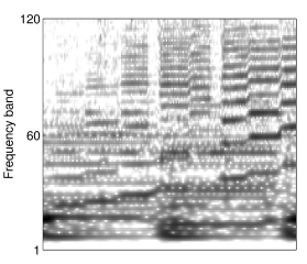
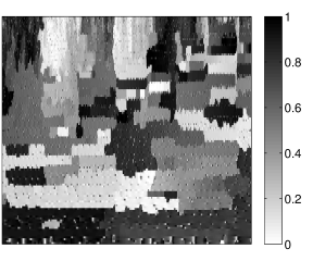
Figure 1: Filter bank spectrogram (l) and difference between original and FBPGHI-restored phase (r) for an excerpt of $s_{4}$. The displayed phase difference is the difference between the phase angles in radians, divided by $\pi$.

FB	(1)	(2)	(3)	(4)	(5)
$a$	8	36	20	73	33
$R$	10.75	9.44	26.40	8.00	21.58

Table I: Decimation factor and redundancy for the considered filter banks.

FB	$s_{1}$	$s_{2}$	$s_{3}$	$s_{4}$	$s_{5}$	$s_{6}$	$s_{7}$
(1)	$-25.65$	$-24.87$	$-12.25$	$-20.22$	$-26.61$	$-28.42$	$-26.38$
(2)	$-32.62$	$-28.76$	$-12.89$	$-23.24$	$-26.96$	$-31.44$	$-28.70$
(3)	$-34.75$	$-29.21$	$-14.30$	$-23.96$	$-27.65$	$-30.28$	$-28.49$
(4)	$-34.52$	$-30.76$	$-14.39$	$-23.08$	$-25.70$	$-32.59$	$-29.28$
(5)	$-35.72$	$-31.32$	$-15.93$	$-23.41$	$-28.03$	$-33.15$	$-29.93$

Table II: FBPGHI - Spectral difference values $E_{\text{spec}}$ in dB.

Comparison with iterative methods: In [13, 8], it was shown that, for Gabor transforms, fGLA performs comparably or better than other iterative schemes in terms of spectral difference. Since we have no reason to assume that the situation changes in the filter bank setting, we consider fGLA as reference algorithm. In Figure 2, we provide some examples as to how FBPGHI compares to fGLA iterations for the signals $s_{4}$ to $s_{7}$ and FB(2). Between $30$ and $80$ fGLA steps are necessary to achieve the same $E_{\text{spec}}$ as FBPGHI and any meaningful improvement requires a large number of additional fGLA steps. Note that every step of fGLA requires $1$ application each of FB synthesis and analysis. Therefore, every iteration has considerable computational cost, while FBPGHI is very efficient, see also [13] for more details. In the same contribution, it was shown that the initialization of fGLA with PGHI provided a significant quality boost over both methods. We expect the same for FBPGHI.

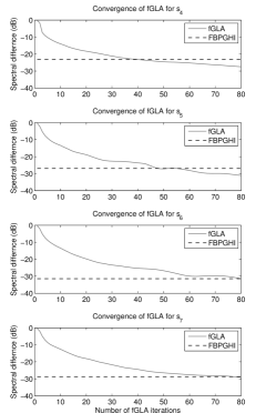
Figure 2: Comparison of fGLA convergence and FBPGHI. Results were obtained with FB(2).

Perceptual performance: Informal listening of the signals restored by the proposed FBPGHI algorithm or $80$ fGLA iterations, for signals $s_{1}$ through $s_{7}$ and FBs (1) to (5) led to the conclusion that both methods performed comparably and without significant artifacts on all signals. No clear performance gap between the algorithms could be detected, with the exception of FB(1) which produced clearly audible artifacts for both FBPGHI and fGLA, albeit on different signals. We attribute these artifacts to the poor frequency resolution of FB(1).

VII Conclusions and Outlook

We have provided an extension of the recent PGHI algorithm for phase reconstruction to filter banks with controlled frequency variation and uniform decimation. Experiments have shown that the algorithm performs competitively in terms of an established objective error measure and also perceptually.

A significant drawback of the proposed method is the required redundancy, in particular for filter banks with highly varying filter bandwidths, see Table II FBs (3),(5). Therefore, a logical next step will be the combination of the heap integration method with nonuniform decimation. Such a scheme will enable the selection of an appropriate sampling step for each frequency channel. Therefore, it can be expected that redundancy is significantly reduced without meaningful impact to the restoration quality. However, the adaptation of the heap integration method to a truly nonuniform sampling grid requires significant work.

In [25], the authors propose an improved phase vocoder based on PGHI for time-stretching and pitch-shifting. A similar application of FBPGHI is conceivable and might possibly further improve the quality of the achieved effect. Future theoretic work could be concerned with finding an appropriate estimate including the neglected terms in (8) as well as estimates for the error if the used filters differ from the Gaussian. Preliminary results have shown promising results for Blackman filters.

References

- [1] R. W. Gerchberg and W. O. Saxton, “A practical algorithm for the determination of the phase from image and diffraction plane pictures,” Optik, vol. 35, pp. 237–246, 1972.
- [2] D. Gunawan and D. Sen, “Iterative phase estimation for the synthesis of separated sources from single-channel mixtures,” IEEE Signal Processing Letters, vol. 17, no. 5, pp. 421–424, May 2010.
- [3] J. Laroche and M. Dolson, “Improved phase vocoder time-scale modification of audio,” IEEE Trans. Speech and Audio Process.,, vol. 7, no. 3, pp. 323–332, May 1999.
- [4] Y. Wang, R. J. Skerry-Ryan, D. Stanton, Y. Wu, R. J. Weiss, N. Jaitly, Z. Yang, Y. Xiao, Z. Chen, S. Bengio, Q. V. Le, Y. Agiomyrgiannakis, R. Clark, and R. A. Saurous, “Tacotron: A fully end-to-end text-to-speech synthesis,” CoRR, vol. abs/1703.10135, 2017. [Online]. Available: http://arxiv.org/abs/1703.10135
- [5] P. Smaragdis, B. Raj, and M. Shashanka, “Missing data imputation for time-frequency representations of audio signals,” Journal of Signal Processing Systems, vol. 65, no. 3, pp. 361–370, 2011.
- [6] R. Balan, P. Casazza, and D. Edidin, “On signal reconstruction without phase,” Applied and Computational Harmonic Analysis, vol. 20, no. 3, pp. 345 – 356, 2006.
- [7] D. Griffin and J. Lim, “Signal estimation from modified short-time Fourier transform,” IEEE Trans. on Acoustics, Speech and Signal Processing, vol. 32, no. 2, pp. 236–243, Apr 1984.
- [8] N. Perraudin, P. Balazs, and P. Søndergaard, “A fast Griffin-Lim algorithm,” in IEEE Workshop on Applications of Signal Processing to Audio and Acoustics (WASPAA),, Oct 2013, pp. 1–4.
- [9] R. Decorsiere, P. Søndergaard, E. MacDonald, and T. Dau, “Inversion of auditory spectrograms, traditional spectrograms, and other envelope representations,” IEEE/ACM Trans. on Audio, Speech, and Language Processing,, vol. 23, no. 1, pp. 46–56, Jan 2015.
- [10] J. Le Roux, H. Kameoka, N. Ono, and S. Sagayama, “Fast signal reconstruction from magnitude STFT spectrogram based on spectrogram consistency,” in Proc. 13th Int. Conf. on Digital Audio Effects (DAFx-10), Sep. 2010, pp. 397–403.
- [11] X. Zhu, G. T. Beauregard, and L. Wyse, “Real-time signal estimation from modified short-time Fourier transform magnitude spectra,” IEEE Trans. on Audio, Speech, and Language Processing,, vol. 15, no. 5, pp. 1645–1653, July 2007.
- [12] G. T. Beauregard, M. Harish, and L. Wyse, “Single pass spectrogram inversion,” in IEEE Int. Conf. Digital Signal Processing (DSP),, July 2015, pp. 427–431.
- [13] Z. Průša, P. Balazs, and P. L. Søndergaard, “A Noniterative Method for Reconstruction of Phase from STFT Magnitude,” IEEE/ACM Trans. on Audio, Speech, and Lang. Process., vol. 25, no. 5, May 2017.
- [14] M. R. Portnoff, “Magnitude-phase relationships for short-time Fourier transforms based on Gaussian analysis windows,” in Proc. ICASSP-79, vol. 4, Apr 1979, pp. 186–189.
- [15] M. S. Jakobsen and J. Lemvig, “Reproducing formulas for generalized translation invariant systems on locally compact abelian groups,” Trans. Amer. Math. Soc., vol. 368, pp. 8447–8480, 2016.
- [16] H. Bölcskei, F. Hlawatsch, and H. G. Feichtinger, “Frame-theoretic analysis of oversampled filter banks,” IEEE Trans. Signal Process., vol. 46, no. 12, pp. 3256–3268, 1998.
- [17] K. Gröchenig, “Acceleration of the frame algorithm,” IEEE Trans. SSP, vol. 41/12, pp. 3331–3340, 1993.
- [18] T. Necciari, N. Holighaus, P. Balazs, Z. Průša, and P. Majdak, “Can frames provide gammatone filter banks with perfect reconstruction?” subm., 2017.
- [19] F. Auger, E. Chassande-Mottin, and P. Flandrin, “On phase-magnitude relationships in the short-time Fourier transform,” IEEE Signal Processing Letters, vol. 19, no. 5, pp. 267–270, May 2012.
- [20] Z. Průša and P. L. Søndergaard, “Real-Time Spectrogram Inversion Using Phase Gradient Heap Integration,” in Proc. Int. Conf. Digital Audio Effects (DAFx-16), Sep 2016.
- [21] J. W. J. Williams, “Algorithm 232: Heapsort,” Communications of the ACM, vol. 7, no. 6, pp. 347–348, 1964.
- [22] “Tech 3253: Sound Quality Assessment Material recordings for subjective tests,” Eur. Broadc. Union, Geneva, Tech. Rep., Sept. 2008.
- [23] B. R. Glasberg and B. C. J. Moore, “Derivation of auditory filter shapes from notched-noise data,” Hear. Res., vol. 47, pp. 103–138, 1990.
- [24] N. Holighaus, M. Dörfler, G. A. Velasco, and T. Grill, “A framework for invertible, real-time constant-Q transforms,” IEEE Trans. Audio Speech Lang. Process., vol. 21, no. 4, pp. 775 –785, 2013.
- [25] Z. Průša and N. Holighaus, “Phase Vocoder Done Right,” in Proc. 25th European Signal Processing Conference (EUSIPCO–2017), Aug 2017.