SQuant: On-the-Fly Data-Free Quantization via Diagonal Hessian Approximation

Abstract

Quantization of deep neural networks (DNN) has been proven effective for compressing and accelerating DNN models. Data-free quantization (DFQ) is a promising approach without the original datasets under privacy-sensitive and confidential scenarios. However, current DFQ solutions degrade accuracy, need synthetic data to calibrate networks, and are time-consuming and costly. This paper proposes an on-the-fly DFQ framework with sub-second quantization time, called SQuant, which can quantize networks on inference-only devices with low computation and memory requirements. With the theoretical analysis of the second-order information of DNN task loss, we decompose and approximate the Hessian-based optimization objective into three diagonal sub-items, which have different areas corresponding to three dimensions of weight tensor: element-wise, kernel-wise, and output channel-wise. Then, we progressively compose sub-items and propose a novel data-free optimization objective in the discrete domain, minimizing Constrained Absolute Sum of Error (or CASE in short), which surprisingly does not need any dataset and is even not aware of network architecture. We also design an efficient algorithm without back-propagation to further reduce the computation complexity of the objective solver. Finally, without fine-tuning and synthetic datasets, SQuant accelerates the data-free quantization process to a sub-second level with $>30\%$ accuracy improvement over the existing data-free post-training quantization works, with the evaluated models under 4-bit quantization. We have open-sourced the SQuant framework.

1 Introduction

With the widespread application of DNN, more and more DNN models are deployed on both computation-constrained and memory-constrained environments, e.g., smartphones, IoT devices, and self-driving cars. The desire for lightweight and energy-efficient DNN deployment solutions is increasing. Quantization is one of the most promising techniques to convert weights and activations to lower bit formats and simultaneously reduce computational time and memory consumption. There are two kinds of quantization: Post-training quantization (PTQ) (Banner et al., 2018; Choukroun et al., 2019; Zhao et al., 2019; Nagel et al., 2020) and Quantization-aware training (QAT) (Gupta et al., 2015; Jacob et al., 2018; Wang et al., 2019; Zhuang et al., 2021). QAT requires to simulate quantization in the training process, which invokes time-consuming retraining and hyper-parameter tuning. In contrast, PTQ directly quantizes well-trained models without retraining. However, they still need training datasets to calibrate (Nagel et al., 2020) quantized models but are often unavailable due to privacy and security issues, such as medical and confidential scenarios.

In contrast, data-free quantization (DFQ) has recently been presented as a promising way to quantize models without original datasets (Nagel et al., 2019; Cai et al., 2020; Zhang et al., 2021; Xu et al., 2020; Liu et al., 2021; Qin et al., 2021; Choi et al., 2020). From a deployment perspective, DFQ is the most attractive quantization method since we can apply it to any trained models as a black box post-processing step. However, current DFQ methods cannot achieve high accuracy and fast processing time simultaneously. Traditionally, DFQ (Nagel et al., 2019) uses rounding quantization, leading to the rounding-to-nearest strategy. Such a strategy causes significant accuracy loss, especially in low-bit settings. To bridge the accuracy gap between data-free and data-driven quantization, researchers propose a series of data-generative DFQ methods. They use gradient-based methods to generate fake datasets for trained models. With the synthetic data, they can employ a data-driven calibration and fine-tuning strategy to improve accuracy. However, data generation typically adopts the time-consuming gradient-based methods, which require multiple iterations to generate each input. For example, prior works often spend hours generating a calibration dataset and fine-tuning the network (Xu et al., 2020; Liu et al., 2021; Zhang et al., 2021).

To solve this dilemma, we propose SQuant, a fast and accurate data-free quantization framework for convolutional neural networks, employing the constrained absolute sum of error (CASE) of weights as the rounding metric. By leveraging Hessian information of network loss due to quantization, we propose a novel diagonal Hessian approximation, which decomposes the optimization objective into three data-free sub-items: element-wise, kernel-wise, and output channel-wise, each of which corresponds to a single or a set of dimensions of the weight tensor. We progressively compose and optimize these three sub-items in the discrete space. The final approximate objective eliminates the requirement of data generation. We propose a progressive algorithm with linear complexity to solve the optimization objective, further accelerating DFQ time to a sub-second level. For example, SQuant only needs an average of 4 ms and 84 ms for quantizing a layer and the overall network of ResNet18, respectively. As it does not require back-propagation nor fine-tuning, SQuant can run on inference-only devices with limited computation and memory resources on the fly. That opens up new opportunities and scenarios for adopting quantization.

Compared with state-of-the-art DFQ methods, SQuant achieves higher accuracy on all evaluated models under the 4/6/8-bit settings. SQuant only introduces 0.1% accuracy loss on average under the 8-bit setting. Under fewer bit precisions, the advantage of SQuant further expands. SQuant only introduces 1.8% accuracy loss on average under the 6-bit setting. Under the 4-bit setting, SQuant can achieve more than 30% accuracy improvement compared with data-free PTQ methods. In a word, SQuant pushes the accuracy and processing time of DFQ to a new frontier.

2 Preliminaries

2.1 Notations

We specifically use ${x}$, ${y}$ and $w$ to denote the input, output, and weight variables, respectively. Constant and scalar are denoted by italic letters, e.g., ${c},M$. Column vector and flattened matrix are denoted by bold lowercase letters, e.g., $\mathbf{w}$, and matrices (or tensors) are represented by uppercase letters, e.g., $\mathbf{W}$. The subscript and superscript can further represent the element indices and the layer of a network, respectively, e.g., $\mathbf{W}^{\ell}_{i,j}$. $\mathop{\mathbb{E}}[\cdot]$ denotes the expectation operator, and the network loss function is represented by $\mathcal{L}(\cdot)$. For convenience in this paper, we call the row of FC (fully connected layer) weight as the output channel and the column of FC weight as the input channel, which are the counterparts to Conv (convolution layer) weight. We use $M$, $N$, and $K$ to denote output channel size, input channel size, and kernel height $\times$ kernel width, respectively. Specifically, FC has the shape of $(M,N,1)$.

2.2 Quantization

Most previous works adopt the rounding-to-nearest approach for quantizing deep neural networks by rounding elements $w$ to the nearest quantization grid values with a fixed-point data type. The quantization and dequantization for a quantized element $\widehat{{w}}$ can be described as $\widehat{{w}}={s}\cdot\text{clip}(\lfloor\frac{{w}}{{s}}\rceil,{min},{max})$, where ${s}$ denotes the quantization scale parameter and, ${min}$ and ${max}$ are the lower and upper thresholds for the clipping function $\text{clip}(\cdot)$. The operator $\lfloor\cdot\rceil$ represents the rounding-to-nearest, i.e., minimizing the mean squared error (MSE) between the quantized and the original value.

2.3 Hessian-Based Optimization for Neural Networks

The Hessian-based approach is one of the most promising optimizations to further improve the quantization (Dong et al., 2019b; a; Nagel et al., 2020; Shen et al., 2020; Qian et al., 2020; Wu et al., 2020; Hubara et al., 2020; Li et al., 2021; Yao et al., 2021) and pruning (Yu et al., 2021) performance for DNN models. Some of those works exploit the Hessian matrix to approximate loss degradation due to the quantization perturbation of weight, $\Delta\mathbf{W}$, by

$$\mathop{\mathbb{E}}[\mathcal{L}(\mathbf{X},\mathbf{Y},\mathbf{W}+\Delta\mathbf{W})-\mathcal{L}(\mathbf{X},\mathbf{Y},\mathbf{W})]{\approx}\mathop{\mathbb{E}}[\Delta\mathbf{W}\cdot{\mathbf{g}^{\mathbf{W}}}+\frac{1}{2}\Delta\mathbf{W}\cdot{\mathbf{H}^{\mathbf{W}}}\cdot\Delta\mathbf{W}^{T}],$$ (1)

where the equation comes from second-order Taylor series expansion, ${\mathbf{g}^{\mathbf{W}}}$ is the gradient and ${\mathbf{H}^{\mathbf{W}}}$ is the full network Hessian matrix w.r.t. original weight, $\mathbf{W}$. Since a well-trained model has already converged, the gradient term will be close to $0$ and thus can be safely ignored. However, computing ${\mathbf{H}^{\mathbf{W}}}$ is infeasible because of the large memory overhead and computation complexity. To tackle this problem, we approximate ${\mathbf{H}^{\mathbf{W}}}$ as a layer-wise Hessian matrix ${\mathbf{H}^{\mathbf{W}^{\ell}}}$ under the assumption of cross-layer independence (Dong et al., 2017; Nagel et al., 2020), i.e., ${\mathbf{H}^{{\mathbf{W}^{\ell}}}}={\mathbf{x}^{\ell}}{{\mathbf{x}^{\ell}}}^{T}\otimes\nabla^{2}_{{\mathbf{y}^{\ell}}}\mathcal{L}$, where $\otimes$ denotes Kronecker product of two matrices, $\nabla^{2}_{{\mathbf{y}^{\ell}}}\mathcal{L}$ is the Hessian of the task loss w.r.t. ${\mathbf{y}^{\ell}}$.

For the $m$-th output channel of Conv or FC, ${\mathbf{H}^{{\mathbf{W}^{\ell}}}}$ can be approximatively simplified into output channel-wise (Nagel et al., 2020; Yu et al., 2021; Wu et al., 2020; Qian et al., 2020),

$${\mathbf{H}^{\mathbf{W}^{\ell}_{m}}}\approx\nabla^{2}_{{\mathbf{y}^{\ell}}}\mathcal{L}_{m,m}\cdot{\mathbf{x}^{\ell}}{{\mathbf{x}^{\ell}}}^{T}=l_{m}\cdot{\mathbf{x}^{\ell}}{{\mathbf{x}^{\ell}}}^{T},$$ (2)

where $\nabla^{2}_{{\mathbf{y}^{\ell}}}\mathcal{L}$ is approximately a diagonal matrix. Then the final optimization objective is

$$\Delta\widehat{\mathbf{W}}^{\ell}_{m,:}= \operatorname*{arg\,min}_{\Delta\mathbf{W}^{\ell}_{m,:}}\quad\Delta\mathbf{W}^{\ell}_{m,:}\mathop{\mathbb{E}}[{\mathbf{H}^{\mathbf{W}^{\ell}_{m}}}]{\Delta\mathbf{W}^{\ell}_{m,:}}^{T}$$ (3)

$$= \operatorname*{arg\,min}_{\Delta\mathbf{W}^{\ell}_{m,:}}\quad\Delta\mathbf{W}^{\ell}_{m,:}\mathop{\mathbb{E}}[{\mathbf{x}^{\ell}}{{\mathbf{x}^{\ell}}}^{T}]{\Delta\mathbf{W}^{\ell}_{m,:}}^{T}=\operatorname*{arg\,min}_{\Delta\mathbf{W}^{\ell}_{m,:}}\mathop{\mathbb{E}}[(\Delta\mathbf{W}^{\ell}_{m,:}{\mathbf{x}^{\ell}})^{2}],$$ (4)

which is the MSE between the output activation produced from original and quantized weights. Each sub-problem deals with a single output channel $\Delta\mathbf{W}^{\ell}_{m,:}$. We will further approximate Eq. (4) to remove any input data dependency from the optimization objective in Sec. 3.2.

3 Methodology

3.1 Overview

Although we can obtain a good quantization strategy by minimizing MSE for each output channel, it is an NP-hard combinatorial optimization problem. Even approaching an acceptable local minimum requires significant effort and involves input activations without the data-free promise.

To avoid the combinatorial optimization problem and eliminate the requirement of data, we propose the SQuant framework. First, SQuant approximates Eq. (4) with three diagonal Hessian matrices corresponding to the dimensions of weight, in Sec. 3.2. Due to the quantization with a fixed-point data type, SQuant transforms the problem into a data-free optimization problem in the discrete domain. SQuant dedicates to optimizing each layer’s weight employing a flipping approach (Nagel et al., 2020) without any input activation. To achieve our proposed optimization objective, minimizing CASE (Constrained Absolute Sum of Error), SQuant progressively composes three approximate sub-items under constraint relaxation, introduced in Sec. 3.3. Finally, SQuant needs to work out a flipping set $\mathbf{f}$ to minimize the CASE of each kernel and output channel. We design an efficient algorithm with a linear computation complexity to find a proper $\mathbf{f}$ based on Eq. (8), in Sec. 3.4.

3.2 Diagonal Hessian Approximation

In this work, we propose a new approximation of the Hessian matrix to cover non-diagonal elements and decompose Eq. (4) into three sub-items that correspond to the three dimensions of the weight tensor as illustrated in Fig. 1: SQuant-E for element-wise optimization covers the diagonal elements of ${\mathbf{H}^{\mathbf{w}^{\ell}_{m}}}$ (H-E); SQuant-K for kernel-wise optimization covers the diagonal blocks of ${\mathbf{H}^{\mathbf{w}^{\ell}_{m}}}$ (H-K); SQuant-C for output channel-wise optimization covers the whole ${\mathbf{H}^{\mathbf{w}^{\ell}_{m}}}$ (H-C).

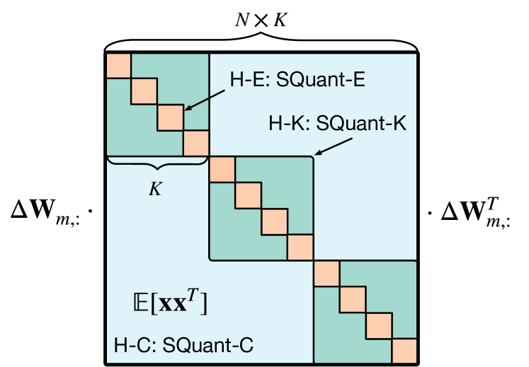
Figure 1: $\Delta\mathbf{W}_{m,:}\mathop{\mathbb{E}}[\mathbf{x}\mathbf{x}^{T}]{\Delta\mathbf{W}_{m,:}}^{T}$. SQaunt-E, SQaunt-K, and SQuant-C are three approximate sub-items, which cover H-E, H-K and H-C, respectively.

The $\mathop{\mathbb{E}}[{\mathbf{x}^{\ell}}{{\mathbf{x}^{\ell}}}^{T}]$ can be approximated by the following equation:

$$\mathop{\mathbb{E}}[{\mathbf{x}^{\ell}}{{\mathbf{x}^{\ell}}}^{T}]\approx\mathbf{E}+\mathbf{K}+\mathbf{C},$$ (5)

where $\mathbf{C}=c_{m}\mathbf{J}_{NK}$,

$$\mathbf{K}=\begin{bmatrix}k_{1}\mathbb{J}_{K}&&\\ &\ddots&\\ &&k_{N}\mathbb{J}_{K}\end{bmatrix}\text{, and }\mathbf{E}=\begin{bmatrix}e_{1,1}&&\\ &\ddots&\\ &&e_{N,K}\end{bmatrix}.$$

In the above equations, $\mathbb{J}_{NK}$ is an all-one matrix with the dimension of $N\times K$ (denoted as $NK$), and $c_{m}$ is a constant value for $m$-th output channel. $\mathbf{K}$ is a diagonal block matrix, where $\mathbb{J}_{K}$ represents an all-one matrix with the dimension of $K\times K$. The $n$-th diagonal block corresponds to $n$-th kernel in convolution and has its own constant value $k_{n}$. $\mathbf{E}$ is a diagonal matrix with the diagonal elements of $e_{n,i}$, each of which is a constant value corresponding to $i$-th element of $n$-th kernel.

Eq. (5) provides an approximation that preserves as much information from three different levels of $\mathop{\mathbb{E}}[{\mathbf{x}^{\ell}}{{\mathbf{x}^{\ell}}}^{T}]$ as possible, which we explain in Appendix A.1. The matrix $\mathbf{C}$ catches the common component of the Hessian matrix, while the matrix $\mathbf{E}$ reserves the individual components in the diagonal line of the Hessian matrix. In addition, we consider kernel-wise approximation for convolution layers by using matrix $\mathbf{K}$. For each inference, the weights of a kernel, $\mathbf{W}^{\ell}_{m,n,:}$, scan the same feature map. As a result, the corresponding $\mathbf{x}$ has nearly the same expectation values in the center area, with a small perturbation in the marginal area due to padding. Therefore, $k_{n}\mathbb{J}_{K}$ as a kernel-wise approximation achieves a low approximate error for convolution. For any $\mathop{\mathbb{E}}[{\mathbf{x}^{\ell}}{{\mathbf{x}^{\ell}}}^{T}]$, we can always find a decomposition that satisfies $e_{n,i},k_{n},c_{m}>0$, for which we present the decomposition method in Appendix A.2. Substituting Eq. (5) into Eq. (4) yields the following equation.

$$\begin{split}\Delta\mathbf{W}^{\ell}_{m,:}\mathop{\mathbb{E}}[{\mathbf{x}^{\ell}}{{\mathbf{x}^{\ell}}}^{T}]{\Delta\mathbf{W}^{\ell}_{m,:}}^{T}\approx\sum_{n,i}e_{n,i}{\Delta\mathbf{W}^{\ell}_{m,n,i}}^{2}+\sum_{n}k_{n}\Delta\mathbf{W}^{\ell}_{m,n,:}\mathbb{J}_{K}{\Delta\mathbf{W}^{\ell}_{m,n,:}}^{T}+c_{m}\Delta\mathbf{W}^{\ell}_{m,:}\mathbb{J}_{NK}{\Delta\mathbf{W}^{\ell}_{m,:}}^{T}.\end{split}$$ (6)

3.3 Data-free Optimization

To achieve the data-free optimization objective, we omit the coefficients ($e_{n,i}$, $k_{n}$ and $c_{m}$) in Eq. (6), which leads to the approximate objective in Eq. (8) optimized by our fast SQuant framework. We present the omitting process and empirically verify that the approximation does almost not influence the performance in Appendix A.2 and Appendix A.3. It can be easily found that there are no training samples needed to minimize,

$$\operatorname*{arg\,min}_{\Delta\mathbf{W}^{\ell}_{m,:}}\quad\sum_{n,i}{\Delta\mathbf{W}^{\ell}_{m,n,i}}^{2}+\sum_{n}{\Delta\mathbf{W}^{\ell}_{m,n,:}\mathbb{J}_{K}{\Delta\mathbf{W}^{\ell}_{m,n,:}}^{T}}+\Delta\mathbf{W}^{\ell}_{m,:}\mathbb{J}_{NK}{\Delta\mathbf{W}^{\ell}_{m,:}}^{T}$$ (7)

$$= \operatorname*{arg\,min}_{\Delta\mathbf{W}^{\ell}_{m,:}}\quad\sum_{n,i}{\Delta\mathbf{W}^{\ell}_{m,n,i}}^{2}+\sum_{n}{{(\sum_{i}\Delta\mathbf{W}^{\ell}_{m,n,i})}^{2}}+{{(\sum_{n,i}\Delta\mathbf{W}^{\ell}_{m,n,i})}^{2}}.$$ (8)

Next, we transform the overall objective Eq. (8) in the discrete space and explain how to compose and optimize the three approximated sub-items in order. Without loss of generality, we assume all weights have been scaled with the scale parameter $s_{m}$ for $\mathbf{W}^{\ell}_{m,:}$.

Sub-item Analysis

For the element-wise item, i.e., the first item in Eq. (8), the problem is reduced to the following objective, which we call SQuant-E.

$$\Delta\widehat{\mathbf{W}}^{\ell}_{m,:}=\operatorname*{arg\,min}_{\Delta\mathbf{W}^{\ell}_{m,:}}\sum_{n,i}{\Delta\mathbf{W}^{\ell}_{m,n,i}}^{2}=\operatorname*{arg\,min}_{\Delta\mathbf{W}^{\ell}_{m,n,i}}{|\Delta\mathbf{W}^{\ell}_{m,n,i}|}\Leftrightarrow\forall\Delta\widehat{\mathbf{W}}^{\ell}_{m,n,i},\ \lvert\Delta\widehat{\mathbf{W}}^{\ell}_{m,n,i}\rvert\leq r_{e}=0.5,$$ (9)

SQuant-E is essentially the rounding method when $r_{e}=0.5$. Rounding does not introduce any approximate error and has $O(1)$ complexity for each weight element. However, as many previous works pointed out (Nagel et al., 2020), rounding-to-nearest is not optimal because it only considers the diagonal elements the matrix $\mathop{\mathbb{E}}[{\mathbf{x}^{\ell}}{{\mathbf{x}^{\ell}}}^{T}]$ while ignores the rest majority elements.

For kernel-wise item (the second item in Eq. (8)), we have the following objective called SQuant-K,

$$\Delta\widehat{\mathbf{W}}^{\ell}_{m,:}=\operatorname*{arg\,min}_{\Delta\mathbf{W}^{\ell}_{m,:}}\sum_{n}{(\sum_{i}\Delta\mathbf{W}^{\ell}_{m,n,i})}^{2}=\operatorname*{arg\,min}_{\Delta\mathbf{W}^{\ell}_{m,n,:}}{|\sum_{i}\Delta\mathbf{W}^{\ell}_{m,n,i}|}\Leftrightarrow \forall\Delta\widehat{\mathbf{W}}^{\ell}_{m,n,:},\ \lvert\sum_{i}\Delta\widehat{\mathbf{W}}^{\ell}_{m,n,i}\rvert\leq r_{k}=0.5,$$ (10)

where $|\sum_{i}\Delta\mathbf{W}^{\ell}_{m,n,i}|$ is the Absolute Sum of Error (ASE) of each kernel-wise weight matrix in the convolution and $r_{k}$ equals 0.5 because of the discrete quantization. In other words, SQuant is based on the insight of Sum of (Signed) error instead of the accumulation of absolute (unsigned) error.

Similarly, for the output channel-wise item (the third item in Eq. (8)), we have SQuant-C,

$$\Delta\widehat{\mathbf{W}}^{\ell}_{m,:}=\operatorname*{arg\,min}_{\Delta\mathbf{W}^{\ell}_{m,:}}{(\sum_{n,i}\Delta\mathbf{W}^{\ell}_{m,n,i})^{2}}\Leftrightarrow \forall\Delta\widehat{\mathbf{W}}^{\ell}_{m,:},\ \lvert\sum_{n,i}\Delta\widehat{\mathbf{W}}^{\ell}_{m,n,i}\rvert\leq r_{c}=0.5.$$ (11)

Relaxation

Obviously, $r_{e}=0.5$ is against $r_{k}=0.5$ because rounding ($r_{e}=0.5$) only guarantees the upper-bound $\dot{r_{k}}=0.5K$ for SQuant-K. Some elements need to relax the constraint $r_{e}$ to a larger number, such as $1.0$, to satisfy $r_{k}=0.5$. Similarly, SQuant-C also needs to relax $r_{k}=1.0$.

CASE Flipping

We adopt the flipping approach (Nagel et al., 2020) to minimize the ASE. Due to the discrete quantization, rounded elements can be flipped (from rounding up to rounding down and vice versa) with $\pm 1$ integer mutation. Formally, we need to work out a flipping set $\mathbf{f}_{m}$ to satisfy the overall objective Eq. (8) by composing these three sub-items in order (SQuant-E $\rightarrow$ SQuant-K $\rightarrow$ SQuant-C) with constraints relaxation. After optimization, the $\mathbf{f}_{m}$ will be

$$\forall(m,n,i)\notin\mathbf{f}_{m},\ \lvert\Delta\mathbf{W}^{\ell}_{m,n,i}\rvert\leq 0.5;\quad\forall(m,n,j)\in\mathbf{f}_{m},\ 0.5\leq\lvert\Delta\mathbf{W}^{\ell}_{m,n,j}\rvert<1.0,$$ (12)

where $\mathbf{f}_{m}$ is the index set of flipped elements for $m$-th output channel. Specifically, we need to flip $k=\lfloor\text{ASE}\rceil$ elements, whose perturbation has the same sign as $\sum_{i}\Delta\mathbf{W}^{\ell}_{m,n,i}$. We prove the equivalence for Eq. (10) and Eq. (11) by illustrating the transformation process to a discrete problem in Appendix B.1.

However, any $k$ elements can satisfy Eq. (10) leading to large search space. Fortunately, based on Eq. (9), SQuant-K can select specific $k$ elements with the top-$k$ largest perturbation because they will have the smallest perturbation after flipping under the constraint of SQuant-E. Therefore, we adopt the Constrained ASE (CASE) to optimize the SQuant-E&K composition via the top-$k$ perturbation algorithm, which is the only solution for minimizing the CASE proven in Appendix B.2. Obviously, SQuant-E&K&C needs to “flip” the “SQuanted” kernel after SQuant-E&K. Notice that we can only flip one element for a kernel to satisfy the constraint $r_{k}=1.0$.

The following section will introduce an efficient SQuant algorithm with a linear computation complexity for CASE flipping.

3.4 On-the-Fly SQuant

Progressive Algorithm

We design a progressive algorithm illustrated in algorithm 1 to meet our stated optimization objective, i.e., minimizing the CASE of weight perturbation. The critical insight of the progressive algorithm is to gradually calibrate the deviation from the optimal global solution introduced by the fine-grained diagonal sub-item. To calibrate the SQuant-E, SQuant-K flips certain rounded elements. After the SQuant-K calibration, SQuant-C then further flips SQuanted kernels.

We start by rounding the weight and updating its perturbation to satisfy $r_{e}=0.5$ (Line 4-5). Then we run the SQuant-K (Line 6) to flip specific elements under $r_{e}=1.0$, satisfy $r_{k}=0.5$, and update kernel perturbation (Line 7). The follow-up SQuant-C (Line 8) further flips specific kernels under $r_{k}=1.0$ and satisfy $r_{c}=0.5$. Finally, we derive the quantized weights (Line 9).

Input: Weight tensor $\mathbf{W}$ of layer $\ell$, scale factor $\mathbf{s}$ of layer $\ell$.

Output: Quantized weight tensor $\mathbf{C}$ of layer $\ell$.

1

2foreach $m\in[1,..,M]$ do // SQuant-C: SQuant $M$ output channels.

3       foreach $n\in[1,..,N]$ do // SQuant-K: SQuant $N$ kernels.

4             foreach $i\in[1,...,K]$ do // SQuant-E: Round $K$ elements.

                   $\mathbf{E}_{m,n,i}=\lfloor\mathbf{W}_{m,n,i}/\mathbf{s}_{m}\rceil$ // Scale and SQuant-E (Rounding).

                   $\Delta\mathbf{E}_{m,n,i}=\mathbf{E}_{m,n,i}-\mathbf{W}_{m,n,i}$ // Element perturbation.

5                  

6            

            $\mathbf{K}_{m,n,:}=$ SQuantFlip($\mathbf{E}_{m,n,:}$, $\Delta\mathbf{E}_{m,n,:}$)// SQuant-K.

             $\Delta\mathbf{K}_{m,n,:}=$UpdatePerturbation($\Delta\mathbf{E}_{m,n,:})$ // Kernel perturbation.

7            

      $\mathbf{C}_{m,:}$ = SQuantFlip($\mathbf{K}_{m,:}$, $\Delta\mathbf{K}_{m,:}$) $\cdot\ \mathbf{s}_{m}$// SQuant-C.

8      

return $\mathbf{C}$

Algorithm 1 Progressive SQuant Algorithm.

Flip Algorithm

SQuant-K and SQuant-C can utilize the same flip function. The goal of the flip algorithm is to find a proper element set $\mathbf{f}$ to flip and minimize the CASE depicted in algorithm 2. First, we need to compute the accumulated perturbation ($e$) (Line 2). We select weights with positive perturbation to decrease the positive $e$ and vice versa for negative $e$. Therefore, we set $0$ for the elements with a different sign (Line 3) to disable them. Obviously, we need only $k=\lfloor|e|\rceil$ elements and reduce $|e|<r_{k}=0.5$ (Line 4). Finally, we flip $k$ weights with the largest $|\mathbf{p}|$ (Line 5-6). For now, we have SQuanted the kernel and tuned kernel CASE to $|e|\leq r_{k}=0.5$. Specifically, for FC and Conv with a kernel size of $(1,1)$, we can skip the SQuant-K. As mentioned in Section 3.3, SQuant-C flips only one element in each kernel. Therefore, we update the kernel perturbation (Line 7 of  algorithm 1) for SQuant-C to flip kernel illustrated in Appendix B.3. As a result, SQuant successfully identifies the optimum combination $\mathbf{f}$ under a low computation complexity, which we analyze in Appendix B.4.

Input: Rounded/SQuanted Weight $\mathbf{w}$;

    Weight perturbation $\mathbf{p}$.

Output: Updated Quantized Weight $\mathbf{w}$.

1

2 def SQuantFlip($\mathbf{w}$, $\mathbf{p}$):

3      

4      $e=\sum_{i}\mathbf{p}_{i}$// Accumulated perturbation.

5      

      $\mathbf{p}[e\cdot\mathbf{p}<0]=0$ // Disable Elements/kernels with different sign from $e$.

       $k=\lfloor|e|\rceil$ // Flip $k$ elements/kernels based on the CASE.

       $\mathbf{f}=$ TopK($|\mathbf{p}|$, $k$).indices// Indices of $k$ largest perturbation.

       $\mathbf{w}[\mathbf{f}]$ = Flip($\mathbf{w}[\mathbf{f}]$)// Flip $k$ elements/kernels with same sign as $e$.

6       return $\mathbf{w}$

Algorithm 2 SQuant Flip Algorithm.

On-the-Fly Framework

From the overall perspective of the optimization, SQuant-K has $MN$ sub-problems, while SQuant-C has $M$ sub-problems. Because of the independence of sub-problems, SQuant is friendly for DNN accelerators, e.g., GPU, allowing each sub-problem to be accelerated in parallel. Without the requirement of back-propagation nor fine-tuning, SQuant can run on inference-only devices with constrained computation and memory resources on the fly. That provides new opportunities for optimizing weight quantization. In the next section, we demonstrate the impressive efficiency and accuracy of SQuant.

4 Experiments

For demonstrating the strength of SQuant, we evaluate the SQuant as well as four SOTA methods, DFQ (Nagel et al., 2019), ZeroQ (Cai et al., 2020), DSG (Zhang et al., 2021; Qin et al., 2021), and GDFQ (Xu et al., 2020), with 5 different CNN models including ResNet-18 & 50 (He et al., 2016), Inception V3 (Szegedy et al., 2016), SqueezeNext (Gholami et al., 2018) and ShuffleNet (Zhang et al., 2018) on the golden standard dataset ImageNet (Krizhevsky et al., 2012).

In our experiments, SQuant is dedicated to weight quantization, including setting quantization range and selecting the grid point with per-channel quantization, which is friendly for hardware accelerators. With the BN-based approach, we adopt a simple rounding method and a wide quantization range for activation suggested by DFQ (Nagel et al., 2019) without breaking the data-free premise. We clip activation tensors in a layerwise manner (per-tensor). We utilize a uniform distribution as the initialization for the activation quantization range. All DFQ algorithms are implemented with PyTorch (Paszke et al., 2019) and evaluated on Nvidia GPU A100-40GB. Unless otherwise stated, we employ both weight and activation quantization in all experiments. Also, uniform quantization grids are used in all experiments, and hyper-parameters, e.g., $r_{e}=r_{k}=1.0$ and $r_{c}=0.5$, for all SQuant experiments are the same.

4.1 Comparison to SOTA Methods

Table 2 and Table 2 show the results on the ImageNet datasets for various bit-width choices, comparing our SQuant against other data-free methods. Among these methods, ZeroQ, DSG, and GDFQ are data-generative approaches with back-propagation. The former two are PTQ methods, while the last is a QAT method, which retrains the network with the synthetic data. DFQ is the only true data-free method with weight equalization and bias correction.

Arch	Method	No BP	No FT	W-bit	A-bit	Top-1
ResNet18	Baseline	–	–	32	32	71.47
	DFQ	✓	✓	4	4	0.10
	ZeroQ	✗	✓	4	4	19.09
	DSG	✗	✓	4	4	34.53
	GDFQ	✗	✗	4	4	60.60
	SQuant	✓	✓	4	4	66.14
	DFQ	✓	✓	6	6	67.30
	ZeroQ	✗	✓	6	6	69.84
	DSG	✗	✓	6	6	70.46
	GDFQ	✗	✗	6	6	70.13
	SQuant	✓	✓	6	6	70.74
	DFQ	✓	✓	8	8	69.70
	ZeroQ	✗	✓	8	8	71.43
	GDFQ	✗	✗	8	8	70.68
	SQuant	✓	✓	8	8	71.47
ResNet50	Baseline	–	–	32	32	77.74
	ZeroQ	✗	✓	4	4	7.75
	DSG	✗	✓	4	4	23.10
	GDFQ	✗	✗	4	4	55.65
	SQuant	✓	✓	4	4	70.80
	ZeroQ	✗	✓	6	6	72.93
	DSG	✗	✓	6	6	76.07
	GDFQ	✗	✗	6	6	76.59
	SQuant	✓	✓	6	6	77.05
	ZeroQ	✗	✓	8	8	77.65
	DSG	✗	✓	8	8	77.68
	GDFQ	✗	✗	8	8	77.51
	SQuant	✓	✓	8	8	77.71

Table 1: Results of data-free methods with ResNet18 and ResNet50. “No BP” means that no back-propagation algorithm is used to generate data, “No FT” means no fine-tuning (retraining) for weight quantization.

Arch	Method	No BP	No FT	W-bit	A-bit	Top-1
Inception V3	Baseline	–	–	32	32	78.81
	ZeroQ	✗	✓	4	4	18.20
	GDFQ	✗	✗	4	4	70.39
	SQuant	✓	✓	4	4	73.26
	ZeroQ	✗	✓	6	6	74.94
	GDFQ	✗	✗	6	6	77.20
	SQuant	✓	✓	6	6	78.30
	ZeroQ	✗	✓	8	8	78.78
	GDFQ	✗	✗	8	8	78.62
	SQuant	✓	✓	8	8	78.79
Squeeze Next	Baseline	–	–	32	32	69.38
	ZeroQ	✗	✓	4	4	0.09
	GDFQ	✗	✗	4	4	28.93
	SQuant	✓	✓	4	4	43.45
	ZeroQ	✗	✓	6	6	16.54
	GDFQ	✗	✗	6	6	65.46
	SQuant	✓	✓	6	6	67.34
	ZeroQ	✗	✓	8	8	68.18
	GDFQ	✗	✗	8	8	68.22
	SQuant	✓	✓	8	8	69.22
Shuffle Net	Baseline	–	–	32	32	65.07
	ZeroQ	✗	✓	6	6	35.21
	GDFQ	✗	✗	6	6	60.12
	SQuant	✓	✓	6	6	60.25
	ZeroQ	✗	✓	8	8	64.34
	GDFQ	✗	✗	8	8	64.03
	SQuant	✓	✓	8	8	64.68

Table 2: Results of data-free methods with InceptionV3, SqueezeNext, and ShuffleNet.

Experiments show that SQuant significantly outperforms all other SOTA DFQ methods, even with synthetic dataset calibrating their networks. The 8-bit quantization preserves better network accuracy than the lower-bit quantization does because of higher precision. The benefit of SQuant becomes more prominent as the bit-width decreases. SQuant outperforms the PTQ methods, i.e., DFQ, ZeroQ, and DSG, more than 30% on all models with 4-bit quantization. It is noteworthy that SQuant surpasses GDFQ in all cases and even surpasses more than 15% in ResNet50 under 4-bit quantization, although GDFQ is a quantization-aware training method.

Table 2 and Table 2 also show that GDFQ significantly outperforms ZeroQ and DSG under lower-bit settings (e.g., 4-bit). Since we use the same activation quantization method for evaluating these methods, the results indicate that the weight quantization plays a critical role in the overall model quantization. However, GDFQ requires fine-tuning (FT) with back-propagation (BP). In contrast, SQuant adopts a direct optimization objective of weight perturbation, which does not require fine-tuning nor BP, and still outperforms GDFQ in the 4-bit setting. These results clearly illustrate the advantages of SQuant, a CASE-based optimization framework, which is to minimize the CASE of weight perturbation.

4.2 SQuant Efficiency

The trade-off between efficiency and accuracy is challenging for previous DFQ methods. Before SQuant, DFQ is the fastest one since it does not require back-propagation and fine-tuning, but it performs poorly, especially in low-bit cases. GDFQ performs relatively well but takes hours to complete 400 epochs that produce synthetic data from weights and fine-tune the network. SQuant employs the direct optimization objective, minimizing the CASE of weight perturbation, pushes the quantization procedure to a sub-second level. Table 3 shows the 4-bit quantization time of the five models using SQuant, ZeroQ, and GDFQ. The efficient algorithm design also contributes to the surprising results. Note that the SQuant results in Table 3 are the sum of all layer quantization time, and it will be faster if we quantize layers in parallel. A single layer takes SQuant just 3 milliseconds on average because SQuant does not involve complex algorithms, such as back-propagation and fine-tuning. That means we can implement the SQuant algorithm on inference-only devices such as smartphones and IoT devices and quantize the network on the fly.

Arch	ResNet18	ResNet50	InceptionV3	SqueezeNext	ShuffleNet
Layers	21	54	95	112	50
SQuant Time (ms)	84	188	298	272	121
ZeroQ Time    (s)	38	92	136	109	38
GDFQ Time  (hour)	1.7	3.1	5.7	4.8	1.9

Table 3: SQuant, ZeroQ and GDFQ 4-bit quantization time on GPU A100

Method	W-bit	A-bit	Top-1
Baseline	32	32	71.47
SQuant-E	3	32	2.05
SQuant-E&C	3	32	40.87
SQuant-E&K	3	32	52.07
SQuant-E&K&C	3	32	60.78
SQuant-E	4	32	48.15
SQuant-E&C	4	32	67.14
SQuant-E&K	4	32	68.07
SQuant-E&K&C	4	32	69.75

Table 4: SQuant ablation results with ResNet18.

Method	No BP	No SD	W-bit	A-bit	Top-1
Baseline	–	–	32	32	71.47
ZeroQ + AdaRound	✗	✗	3	32	49.86
DSG + AdaRound	✗	✗	3	32	56.09
SQuant	✓	✓	3	32	60.78
ZeroQ + AdaRound	✗	✗	4	32	63.86
DSG + AdaRound	✗	✗	4	32	66.87
SQuant	✓	✓	4	32	69.75
ZeroQ + AdaRound	✗	✗	5	32	68.39
DSG + AdaRound	✗	✗	5	32	68.97
SQuant	✓	✓	5	32	71.19

Table 5: ResNet18 results of SQuant, ZeroQ and DSG with AdaRound. “No SD” means no synthetic data.

4.3 Ablation study

SQuant Granularity

We decouple the effect of SQuant-K and SQuant-C, which have different granularities to optimize CASE. As shown in Table 5, their accuracies both outperform SQuant-E (i.e., rounding), and combining them leads to higher accuracy for ResNet18. SQuant-E&C has a lower accuracy than SQuant-E&K because SQuant-C has a more significant approximation error than SQuant-K. On the other hand, SQuant-E alone is not optimal because it uses a smaller granularity and ignores a large amount of Hessian information as we analyze in Section 3. This ablation study shows that SQuant-E&K&C achieves the best accuracy by exploiting the most Hessian information (H-C), and SQuant-E&K also achieves a higher accuracy with H-K than SQuant-E with H-E.

Comparison to Data-free AdaRound

AdaRound (Nagel et al., 2020) is a novel data-driven PTQ method, which also utilizes the Hessian-based approach to round-up or round-down the weights with an approximation assumption. Under the data-free premise, we augment ZeroQ and DSG with the AdaRound by feeding their generated synthetic data to AdaRound. Results in Table 5 show that SQuant has better accuracy than data-free AdaRound because SQuant directly optimizes the CASE objective instead of the MSE of the output activation adopted by AdaRound. It is hard for DSG$+$AdaRound to find the optimal solution with an excessively long optimization path and gradient-based approaches. Even though AdaRound tries a shorter way to fine-tune the weights in the layer-wise fashion, SQuant still outperforms AdaRound in quantization time and accuracy.

5 Related Work

Compression is a promising method to reduce the DNN model’s memory and computation cost. Pruning (Han et al., 2015b; a) is one of the effective approaches to exploit the inherent redundancy of DNN. However, pruning will cause sparse irregular memory accesses. Therefore, pruning needs software (Gale et al., 2020; Guan et al., 2020; Qiu et al., 2019; Guo et al., 2020a; Guan et al., 2021; Fedus et al., 2021) and hardware (Gondimalla et al., 2019; Guo et al., 2020b; Zhang et al., 2020; Wang et al., 2021) optimization to accelerate.

Quantization is more practical because it can be supported directly by existing accelerators. Quantization-aware training (QAT) (Gupta et al., 2015; Jacob et al., 2018; Wang et al., 2019; Zhuang et al., 2021) is one of the most promising techniques to retrain networks and mitigate the accuracy drop introduced by quantization. However, the training procedure is time-consuming and costly. Therefore, post-training quantization (PTQ) (Banner et al., 2018; Choukroun et al., 2019; Zhao et al., 2019; Nagel et al., 2020) has earned lots of attention due to the absence of any fine-tuning or retraining process, at the expense of accuracy.

Recently, several methods for CNN quantization without the original training datasets have been proposed. These methods are known as data-free quantization (DFQ), including PTQ (Nagel et al., 2019; Cai et al., 2020; Zhang et al., 2021) and QAT (Xu et al., 2020; Liu et al., 2021; Qin et al., 2021; Choi et al., 2020). DFQ (Nagel et al., 2019) and ACIQ (Nagel et al., 2019) rely on weight equalization or bias correction without requiring synthetic data. Other works synthesize the data to calibrate or fine-tune the network based on the batch normalization statistics (Cai et al., 2020) or adversarial knowledge distillation techniques (Liu et al., 2021; Choi et al., 2020).

6 Conclusion

This paper approximates and composes the original Hessian optimization objective into the CASE of weight perturbation with a data-free premise. Surprisingly, CASE only involves the weight perturbation and requires no knowledge of any datasets or network architecture. Based on that, we proposed the on-the-fly SQuant framework. We used a progressive algorithm to minimize CASE directly and significantly improve accuracy than other DFQ methods. SQuant considerably reduces optimization complexity and accelerates the data-free quantization procedure, which previously requires back-propagation with massive computation and memory resources consumption seen in other works. In summary, SQuant outperforms other data-free quantization approaches in terms of accuracy and pushes the quantization processing time to a sub-second level.

Acknowledgments

We would like to thank the anonymous reviewers for their constructive feedback. This work was supported by the National Key R&D Program of China under Grant 2021ZD0110104, and the National Natural Science Foundation of China (NSFC) grant (U21B2017, 62072297, and 61832006).

Appendix A Approximation and Decomposition

A.1 Approximated Hessian Matrix for data-free quantization

The quantization loss function for the entire network is

$$\mathcal{L}(\Delta\mathbb{W})=\Delta\mathbb{W}\mathop{\mathbb{E}}[{\mathbf{H}}]{\Delta\mathbb{W}}^{T}.$$ (13)

Consider a convolution layer defined as

$$\mathbf{Y}_{m,h,w}=\sum_{n,i,j}{\mathbf{W}_{m,n,i,j}\mathbf{X}_{n,h-i,w-j}}.$$ (14)

Here, $\mathbf{Y}$ has three dimensions, output channel, output feature map height, and output feature map width, i.e., $(M\times OH\times OW)$ indexing by $(m,h,w)$, $\mathbf{W}$ has four dimensions, output channel, input channel, kernel height, kernel width, i.e., $(M\times N\times KH\times KW)$ indexing by $(m,n,i,j)$, and $\mathbf{X}$ has three dimensions, input channel, input feature map height, and input feature map width, i.e., $(N\times IH\times IW)$ indexing by ${(n,h-i,w-j)}$. Ignoring the interaction between layers and output channels following Nagel et al. (2020), for a specific convolution layer $l$ and output channel $m$, the elements of corresponding output channel-wise Hessian ${\mathbf{H}^{\mathbf{W}^{\ell}_{m}}}$ is

$$\mathbf{H}^{\mathbf{W}^{\ell}_{m}}_{n,i,j,n^{\prime},i^{\prime},j^{\prime}}= \frac{\partial^{2}\mathcal{L}}{\partial\mathbf{W}_{m,n,i,j}\partial\mathbf{W}_{m,n’,i’,j’}}$$ (15)

$$= \frac{\partial}{\partial\mathbf{W}_{m,n,i,j}}\sum_{h,w}\frac{\partial\mathcal{L}}{\partial\mathbf{Y}_{m,h,w}}\frac{\partial\mathbf{Y}_{m,h,w}}{\partial\mathbf{W}_{m,n,i,j}}$$ (16)

$$= \frac{\partial}{\partial\mathbf{W}_{m,n,i,j}}\sum_{h,w}\frac{\partial\mathcal{L}}{\partial\mathbf{Y}_{m,h,w}}\mathbf{X}_{n,h-i,w-j}$$ (17)

$$= \sum_{h,w}\left(\frac{\partial}{\partial\mathbf{Y}_{m,h,w}}\frac{\partial\mathcal{L}}{\partial\mathbf{Y}_{m,h’,w’}}\right)\mathbf{X}_{n,h-i,w-j}$$ (18)

$$= \sum_{h,w}\left(\frac{\partial}{\partial\mathbf{Y}_{m,h,w}}\sum_{h^{\prime},w^{\prime}}\frac{\partial\mathcal{L}}{\partial\mathbf{Y}_{m,h^{\prime},w^{\prime}}}\mathbf{X}_{n^{\prime},h^{\prime}-i^{\prime},w^{\prime}-j^{\prime}}\right)\mathbf{X}_{n,h-i,w-j}$$ (19)

$$= \sum_{h,w}\sum_{h^{\prime},w^{\prime}}\frac{\partial^{2}\mathcal{L}}{\partial\mathbf{Y}_{m,h,w}\partial\mathbf{Y}_{m,h^{\prime},w^{\prime}}}\mathbf{X}_{n,h-i,w-j}\mathbf{X}_{n^{\prime},h^{\prime}-i^{\prime},w^{\prime}-j^{\prime}}$$ (20)

Assuming $\nabla^{2}_{{\mathbf{y}^{\ell}}}\mathcal{L}$ is a diagonal matrix yields Eq. (30) in (Nagel et al., 2020)

$$\mathbf{H}^{\mathbf{W}^{\ell}_{m}}_{n,i,j,n^{\prime},i^{\prime},j^{\prime}}\approx \sum_{h,w}\frac{\partial^{2}\mathcal{L}}{\partial\mathbf{Y}_{m,h,w}^{2}}\mathbf{X}_{n,h-i,w-j}\mathbf{X}_{n,h-i^{\prime},w-j^{\prime}}.$$ (21)

To make Eq. (13) get irrelevant to training samples, we assume that input feature maps auto-correlate with each other in a similar way, resulting in

$$\mathop{\mathbb{E}}[\mathbf{H}^{\mathbf{W}^{\ell}_{m}}_{n,i,j,n^{\prime},i^{\prime},j^{\prime}}]= \mathop{\mathbb{E}}[\sum_{h,w}\frac{\partial^{2}\mathcal{L}}{\partial\mathbf{Y}_{m,h,w}^{2}}\mathbf{X}_{n,h-i,w-j}\mathbf{X}_{n^{\prime},h-i^{\prime},w-j^{\prime}}]\approx c_{m}$$ (22)

for all $n,i,j,n^{\prime},i^{\prime}$ and $j^{\prime}$, where $c_{m}$ is a constant. It should be noted that Eq. (22) is a strong assumption. For more accurate approximation, we further look into each input channel (i.e., $n=n^{\prime}$, $i\neq i^{\prime}$, and $j\neq j^{\prime}$), and find

$$\mathop{\mathbb{E}}[\mathbf{H}^{\mathbf{W}^{\ell}_{m,n}}_{i,j,i^{\prime},j^{\prime}}]= \mathop{\mathbb{E}}[\sum_{h,w}\frac{\partial^{2}\mathcal{L}}{\partial\mathbf{Y}_{m,h,w}^{2}}\mathbf{X}_{n,h-i,w-j}\mathbf{X}_{n,h-i^{\prime},w-j^{\prime}}]\approx k_{m,n},$$ (23)

for all $i$, $j$, $i^{\prime}$, and $j^{\prime}$, where $k_{m,n}$ is a constant. It is generally true because the kernel size is usually much smaller than the size of feature maps, so the shift introduced by different $i$, $j$, $i^{\prime}$, and $j^{\prime}$ is a small perturbation of $\mathop{\mathbb{E}}[\mathbf{H}^{\mathbf{W}^{\ell}_{m,n}}_{i,j,i^{\prime},j^{\prime}}]$ compared with the summation over the entire feature map. Finally, we focus on each diagonal element of Hessian matrix (i.e., $n=n^{\prime}$, $i=i^{\prime}$, and $j=j^{\prime}$) and denote

$$\mathop{\mathbb{E}}[\mathbf{H}^{\mathbf{W}^{\ell}_{m,n,i,j}}]= \mathop{\mathbb{E}}[\sum_{h,w}\frac{\partial^{2}\mathcal{L}}{\partial\mathbf{Y}_{m,h,w}^{2}}\mathbf{X}^{2}_{n,h-i,w-j}]=e_{m,n,i,j},$$ (24)

where $e_{m,n,i,j}$ is a constant. Please note that the output channel-wise expected Hessian matrix $\mathop{\mathbb{E}}[\mathbf{H}^{\mathbf{W}^{\ell}_{m}}_{n,i,j,n^{\prime},i^{\prime},j^{\prime}}]$ is a principle submatrix of $\mathop{\mathbb{E}}[\mathbf{H}]$, so it must positive semi-define. Therefore, we set $e_{m,n,i,j}>k_{m,n}>c_{m}>0$ to ensure the approximation to $\mathop{\mathbb{E}}[\mathbf{H}^{\mathbf{W}^{\ell}_{m}}_{n,i,j,n^{\prime},i^{\prime},j^{\prime}}]$ is also positive semi-define and nontrivial. Considering Eq. (22), Eq. (23), and Eq. (24) at the same time, we can get the approximation to expected Hessian shown in Eq. (5). Extending the discussion to fully connected layer is straightforward thus omitted here.

A.2 Decomposition

In this section, we present the decomposition method for $\mathbf{H}^{\mathbf{W}^{\ell}_{m}}=l_{m}\mathop{\mathbb{E}}[{\mathbf{x}^{\ell}}{{\mathbf{x}^{\ell}}}^{T}]$ illustrated in the algorithm 3. First, we construct three matrices with the shape of $(NK,NK)$, $\mathbf{C}^{\prime}=\mathbf{J}_{NK}$,

$$\mathbf{K}^{\prime}=\begin{bmatrix}\mathbb{J}_{K}&&\\ &\ddots&\\ &&\mathbb{J}_{K}\end{bmatrix}\text{, and }\mathbf{E}^{\prime}=\begin{bmatrix}1&&\\ &\ddots&\\ &&1\end{bmatrix}.$$

Here, $\mathbb{J}_{NK}$ is an all-one matrix with dimension $NK=N\times K$ and $\mathbb{J}_{K}$ represents an all-one matrix with dimension $K$. The $n$-th diagonal block corresponds to $n$-th kernel in convolution and has the same constant $k_{n}$. $\mathbf{E}$ is a diagonal matrix whose diagonal elements are 1.

Input: $\mathop{\mathbb{E}}[{\mathbf{x}^{\ell}}{{\mathbf{x}^{\ell}}}^{T}]$, $\mathbf{H}$;

    Channel-wise matrix, $\mathbf{C}^{\prime}$.

    Kernel-wise matrix, $\mathbf{K}^{\prime}$.

    Element-wise matrix, $\mathbf{E}^{\prime}$.

Output: Matrix $\mathbf{E}$,$\mathbf{K}$, and $\mathbf{C}$.

1 $\mathbf{H}^{\prime}=|\mathbf{H}|$

$c_{m}=(1-\epsilon)\cdot\min(\mathbf{H}^{\prime})$ // Output channel-wise.

2 $\mathbf{C}=c_{m}\mathbf{C}^{\prime}$

3 foreach $n\in[1,...,N]$ do // Kernel-wise.

4       $k_{n}=(1-\epsilon^{\prime}_{n})\cdot\min(\mathbf{H}^{\prime}_{n:n+K,\ n:n+K}-c_{m})$

5       $\mathbf{K}_{n,:}=k_{n}\mathbf{K}^{\prime}_{n,:}$

6       foreach $i\in[1,...,K]$ do // Element-wise.

7             $e_{n,i}=\mathbf{H}^{\prime}_{n\times K+i,\ n\times K+i}-c_{m}-k_{n}$

8             $\mathbf{E}_{n,i}=e_{n,i}\mathbf{E}^{\prime}_{n,i}$

9            

10      

return $\mathbf{E},\mathbf{K},\mathbf{C}$

Algorithm 3 $\mathop{\mathbb{E}}[{\mathbf{x}^{\ell}}{{\mathbf{x}^{\ell}}}^{T}]$ Decomposition.

In algorithm 3, $0<$ $\epsilon,\epsilon^{\prime}$ $<1$, and we can get the matrices $\mathbf{E},\mathbf{K}$, and $\mathbf{C}$. Evidently, algorithm 3 can make $c_{m}>0$, $k_{n}>0$, and $e_{n,i}>0$ for any $\mathop{\mathbb{E}}[{\mathbf{x}^{\ell}}{{\mathbf{x}^{\ell}}}^{T}]\approx\mathbf{E}+\mathbf{K}+\mathbf{C}$.

A.3 Approximation Error Analysis

To achieve the data-free optimization objective, we omit the coefficients ($e_{n,i}$, $k_{n}$ and $c_{m}$) in Eq. (6), which leads to the approximate objective in Eq. (8) optimized by our fast SQuant framework. We approximate Eq. (6) to Eq. (8) to enable fast data-free quantization. The approximation error is insignificant as our comprehensive results have shown the high accuracy of the final quantized model in Table 2 and Table 2 of the manuscript. The intuition behind the approximation is that we use an iterative process which progressively reduces each term of Eq. (6). Because each term’s coefficient ($e_{n,i}$, $k_{n}$, and $c_{m}$) is positive, the reduction of each term would generally lead to the reduction of the precise objective in Eq. (6). In this section, we provide an empirical analysis of the approximation error between Eq. (6) andEq. (8).

In this empirical experiment, we use the real dataset to generate the precise coefficients of $e_{n,i}$, $k_{n}$, and $c_{m}$ in Eq. (6). To quantify the approximation error in our SQuant framework, we evaluate a metric called approximation precision and show that we achieve a nearly 95% approximation precision.

Layers	Squant-E&K			Squant-E&K&C
	Flipped	Correct	AP	Flipped	Correct	AP
1	2346	2346	100.00 %	123	123	100.0 %
2	2683	2594	96.68 %	97	97	100.0 %
3	2662	2653	99.66 %	100	100	100.0 %
4	2698	2630	97.48 %	107	107	100.0 %
5	-	-	-	230	220	95.7 %
6	5349	5339	99.81 %	223	223	100.0 %
7	10782	10676	99.02 %	332	332	100.0 %
8	10777	10633	98.66 %	342	342	100.0 %
9	10655	10424	97.83 %	348	348	100.0 %
10	-	-	-	649	619	95.4 %
11	21371	21173	99.07 %	663	663	100.0 %
12	43116	41561	96.39 %	906	906	100.0 %
13	42976	41402	96.34 %	932	932	100.0 %
14	43321	41315	95.37 %	918	918	100.0 %
15	-	-	-	1988	1639	82.4 %
16	86010	83070	96.58 %	1846	1846	100.0 %
17	171344	161358	94.17 %	2629	2629	100.0 %
18	172071	158066	91.86 %	2602	2602	100.0 %
19	172623	154536	89.52 %	2504	2504	100.0 %
Total	800784	749776	93.6 %	17539	17150	97.8 %
Acc.	68.07			69.75

Table 6: ResNet18 results under 4-bit weight-only quantization. “Flipped” is the number of the Flipped elements after SQuant optimization. “Correct” is the number of elements has the same optimization direction as the precise objective. AP is the approximation precision.

Since SQuant uses the flipping-based iterative optimization framework to minimize Eq. (8), we define an element as correctly flipped if its flipping leads to the decrease of the precise objective Eq. (6) and approximate objective Eq. (8). The approximation precision (AP) is the ratio of the correct element based on data-free Eq. (8) compared to data-driven Eq. (6), i.e.,

$$\text{AP}=\frac{\text{Number of correct elements}}{\text{Number of flipped elements}}.$$

We perform the above approximation error analysis on ResNet18 with ImageNet under 4-bit weight-only quantization. We evaluate the SQuanted weight on the inference datasets. We compute the coefficients $e_{n,i}$, $k_{n}$, and $c_{m}$ with 1000 samples. Table 6 shows the results, which clearly show that SQuant-E&K&C achieves nearly 100% approximation precision. In other words, nearly all flipped elements can indeed reduce the precise objective in Eq. (6). Based on this empirical study, we show that the approximation from Eq. (6) to Eq. (8) is effective for our data-free quantization.

Appendix B Squant Algorithm

B.1 Discrete Optimization Problem

We introduce the transformation of the discrete optimization problem. We know that the quantization is to round the scaled elements to the integer grid. Each quantization step has two rounding directions, rounding up and down, with a step size of 1. We have the quantization example within $[0,1]$ shown in Fig. 2.

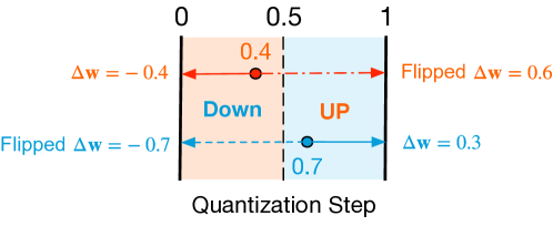
Figure 2: The flipping approach.

Clearly, the element $0.7$ ($0.4$) can be rounded up (down) to $1.0$ ($0.0$) with $+0.3$ ($-0.4$) orignal perturbation and flipped to $0.0$ ($1.0$) with $-0.7$ ($+0.6$) flipped perturbation with $-1$ ($+1$) mutation. Each flipping operation leads to a $\pm 1$ integer mutation and increases the perturbation to $[0.5,1.0]$. We prove that we can always find $k=\lfloor|\sum_{i}\Delta\mathbf{W}^{\ell}_{m,n,i}|\rceil$ elements to flip and reduce $|\sum_{i}\Delta\widehat{\mathbf{W}}^{\ell}_{m,n,i}|\leq 0.5$.

Proof.

Assume $n$-th kernel has $K$ elements, $a$ rounded up elements with index set $\mathbf{f}_{a}$ have positive perturbation, $b$ rounded down elements with index set $\mathbf{f}_{b}$ have negative perturbation, and $K=a+b$. Then, we have

$$|\sum_{i}\Delta\mathbf{W}^{\ell}_{m,n,i}|= \Big{\lvert}\sum_{t}{\Delta\mathbf{W}^{\ell}_{m,n,t}}-\sum_{j}{|\Delta\mathbf{W}^{\ell}_{m,n,j}|}\Big{\rvert},\quad t\in\mathbf{f}_{a},\quad j\in\mathbf{f}_{b}$$ (25)

$$\leq \max(\sum_{t}{\Delta\mathbf{W}^{\ell}_{m,n,t}},\quad\sum_{j}{|\Delta\mathbf{W}^{\ell}_{m,n,j}|}),\quad t\in\mathbf{f}_{a},\quad j\in\mathbf{f}_{b}$$ (26)

Without loss of generality, let $\sum_{t}{\Delta\mathbf{W}^{\ell}_{m,n,t}}>\sum_{j}{|\Delta\mathbf{W}^{\ell}_{m,n,j}|}$,

$$\max(\sum_{t}{\Delta\mathbf{W}^{\ell}_{m,n,t}},\quad\sum_{j}{|\Delta\mathbf{W}^{\ell}_{m,n,j}|})= \sum_{t}{\Delta\mathbf{W}^{\ell}_{m,n,t}}\quad t\in\mathbf{f}_{a},\quad j\in\mathbf{f}_{b}$$ (27)

$$\leq 0.5\cdot a.$$ (28)

Therefore, we can always find $k=\lfloor|\sum_{i}\Delta\mathbf{W}^{\ell}_{m,n,i}|\rceil\leq\lfloor 0.5\cdot a\rceil$ elements in $\mathbf{f}_{a}$ with size of $a$ to flip down and make $|\sum_{i}\Delta\widehat{\mathbf{W}}^{\ell}_{m,n,i}|\leq 0.5$. For example, if $\sum_{i}\Delta\mathbf{W}^{\ell}_{m,n,i}=3.2$, we need to flip 3 elements with positive perturbation (rounding up) to negative (rounding down) with $-3.0$ mutation. Then, we have

$$\Delta\widehat{\mathbf{W}}^{\ell}_{m,n:}=\operatorname*{arg\,min}_{\Delta\mathbf{W}^{\ell}_{m,n,:}}{(\sum_{i}\Delta\mathbf{W}^{\ell}_{m,n,i})^{2}}\Rightarrow\ \lvert\sum_{i}\Delta\widehat{\mathbf{W}}^{\ell}_{m,n,i}\rvert=\Big{\lvert}k-{|\sum_{i}\Delta\mathbf{W}^{\ell}_{m,n,i}|}\Big{\rvert}.$$ (29)

For each kernel $|\sum_{i}\Delta\mathbf{W}^{\ell}_{m,n,i}|\geq 0$, $\sum_{i}\Delta\widehat{\mathbf{W}}^{\ell}_{m,n,i}$ has the minimum value $\Big{\lvert}k-{|\sum_{i}\Delta\mathbf{W}^{\ell}_{m,n,i}|}\Big{\rvert}\leq 0.5$. The sufficiency of Eq. (10) has been proven:

$$\Delta\widehat{\mathbf{W}}^{\ell}_{m,:}=\operatorname*{arg\,min}_{\Delta\mathbf{W}^{\ell}_{m,n,:}}{(\sum_{i}\Delta\mathbf{W}^{\ell}_{m,n,i})^{2}}\Rightarrow \forall\Delta\widehat{\mathbf{W}}^{\ell}_{m,n,:},\ \lvert\sum_{i}\Delta\widehat{\mathbf{W}}^{\ell}_{m,n,i}\rvert\leq r_{k}=0.5$$ (30)

When $a=K,b=0$ and all perturbation $=0.5$, original $\sum_{i}\Delta\mathbf{W}^{\ell}_{m,n,i}$ have the upper bound $0.5\cdot K$. ∎

Proof.

If we flip $k-1$ or $k+1$ elements for $n$-th kernel, the $\sum_{i}\Delta\widehat{\mathbf{W}}^{\ell}_{m,n,i}$ can reduce to $\Big{\lvert}k-1-{|\sum_{i}\Delta\mathbf{W}^{\ell}_{m,n,i}|}\Big{\rvert}$ and $\Big{\lvert}k+1-{|\sum_{i}\Delta\mathbf{W}^{\ell}_{m,n,i}|}\Big{\rvert}$, respectively. Obviously,

$$\Big{\lvert}k-1-{|\sum_{i}\Delta\mathbf{W}^{\ell}_{m,n,i}|}\Big{\rvert}=\Big{\lvert}\lfloor|\sum_{i}\Delta\mathbf{W}^{\ell}_{m,n,i}|\rceil-1-{|\sum_{i}\Delta\mathbf{W}^{\ell}_{m,n,i}|}\Big{\rvert}>0.5,$$ (31)

$$\Big{\lvert}k+1-{|\sum_{i}\Delta\mathbf{W}^{\ell}_{m,n,i}|}\Big{\rvert}=\Big{\lvert}\lfloor|\sum_{i}\Delta\mathbf{W}^{\ell}_{m,n,i}|\rceil+1-{|\sum_{i}\Delta\mathbf{W}^{\ell}_{m,n,i}|}\Big{\rvert}>0.5.$$ (32)

With other numbers $\neq k$, we can also draw the same conclusions. Therefore, when $r_{k}\leq 0.5$, there is only one value, i.e., the minimum value, with $k$ flipped elements satisfy the Eq. (10). The necessity of Eq. (10) has been proven:

$$\operatorname*{arg\,min}_{\Delta\mathbf{W}^{\ell}_{m,n,:}}{(\sum_{i}\Delta\mathbf{W}^{\ell}_{m,n,i})^{2}}\Leftrightarrow \forall\Delta\widehat{\mathbf{W}}^{\ell}_{m,n,:},\ \lvert\sum_{i}\Delta\widehat{\mathbf{W}}^{\ell}_{m,n,i}\rvert\leq r_{k}=0.5$$ (33)

Similarly, we can extend all conclusions to SQuant-C. ∎

For SQuant, we only consider the flipping operation in one quantization step and select the elements whose sign is the same as $\sum_{i}\Delta\mathbf{W}^{\ell}_{m,n,i}$ because flipping with more quantization steps (e.g., flip $0.7$ to $-1.0$) and the elements with different perturbation signs will cause a more significant perturbation and will violate the Eq. (8). We explain that in the next section.

B.2 Proof of Tok-$k$ Perturbation Algorithm

Proof.

We will prove the SQuant-E&K will lead to the top-$k$ algorithm. We have the composition SQuant-E and SQuant-K optimization objective for $n$-th kernel,

$$\operatorname*{arg\,min}_{\Delta\mathbf{W}^{\ell}_{m,n,:}}\quad\sum_{i}{(\Delta\mathbf{W}^{\ell}_{m,n,i})^{2}}+{(\sum_{i}\Delta\mathbf{W}^{\ell}_{m,n,i})^{2}},$$ (34)

which is the first two items of Eq. (8). Without loss of generality, we assume $e=\sum_{i}\Delta\mathbf{W}^{\ell}_{m,n,i}>0$, then SQuant needs to flip $k=\lfloor e\rceil$ elements with perturbation $>0$ to transform $\sum_{i}\Delta\mathbf{W}^{\ell}_{m,n,i}$ to $e-k$ and is still constant $e-k$ regardless of which $k$ elements are. Therefore, the $k$ elements are only determined by the first item of Eq. (34), $\sum_{i}{(\Delta\mathbf{W}^{\ell}_{m,n,i})^{2}}$. We denote $\mathbf{f}$ as the index set of the $k$ flipped elements and the original perturbation $\mathbf{O}=\Delta\mathbf{W}^{\ell}_{m,n,:}$ for $n$-th kernel. Therefore, $\mathbf{O}_{j}>0,\ j\in\mathbf{f}$. Substituting $\mathbf{f}$ and $\mathbf{O}$ in Eq. (34), we have the optimization objective for $\mathbf{f}$ after flipping $k$ elements,

$$\operatorname*{arg\,min}_{\mathbf{f}}\quad\sum_{t}{(|\mathbf{O}_{t}|)^{2}}+\sum_{j}{(1-|\mathbf{O}_{j}|)^{2}}+(e-k)^{2},\quad t\notin\mathbf{f},\ j\in\mathbf{f},\ \mathbf{O}_{j}>0$$ (35)

$$= \operatorname*{arg\,min}_{\mathbf{f}}\quad\sum_{i}{(|\mathbf{O}_{i}|)^{2}}-\sum_{j}{(|\mathbf{O}_{j}|)^{2}}+\sum_{j}{(1-|\mathbf{O}_{j}|)^{2}},\quad j\in\mathbf{f},\ \mathbf{O}_{j}>0$$ (36)

$$= \operatorname*{arg\,min}_{\mathbf{f}}\quad\sum_{j}{[(1-|\mathbf{O}_{j}|)^{2}-|\mathbf{O}_{j}|^{2}]},\quad j\in\mathbf{f},\ \mathbf{O}_{j}>0$$ (37)

$$= \operatorname*{arg\,min}_{\mathbf{f}}\quad\sum_{j}{(1-2|\mathbf{O}_{j}|)},\quad j\in\mathbf{f},\ \mathbf{O}_{j}>0$$ (38)

$$= \operatorname*{arg\,max}_{\mathbf{f}}\quad\sum_{j}{(|\mathbf{O}_{j}|)},\quad j\in\mathbf{f},\ \mathbf{O}_{j}>0.$$ (39)

Therefore, the Eq. (39) is essentially the top-$k$ perturbation algorithm. We can easily extend the top-$k$ algorithm in SQuant-C and design the perturbation update algorithm in  B.3.

∎

B.3 Perturbation Update Algorithm

SQuant-K initializes all rounded elements as flip candidates. After SQuant-K, we update the flip candidates for SQuant-C as shown in algorithm 4 based on the insight of top-$k$ perturbation algorithm ( B.2).

Over SQuant

First we define the situation of $k>\lvert e\rvert$ as “Over SQuant” (line 6). For example, if we have a kernel with $e=+1.6$, we need to SQuant it to $-0.4$ to satisfy in $(-0.5,0.5]$ with flipping $k=2$ elements $\{2.6,2.7\}$ to $\{2,2\}$. Obviously, when SQuant-C needs this kernel to calibrate, the last element $2.7$ should be the first and the only candidate (line 7,8) to flip back to the original rounded number $3$ to make the $e=+0.6$, due to it has the largest element perturbation in the $k$ fliped elements and the smallest element perturbation $(|-0.3|<0.5)$ after it flips back. It is vice versa for $e<0$.

Under SQuant

For “Under SQuant” (line 9), we need to make the first un-flipped element as the flip candidate (line 10, 11) for SQuant-C, and will lead the kernel to ”Over SQuant” with absolute kernel perturbation in $(0.5,1.0)$ when SQuant-C flips this element of the kernel.

Input: Weight perturbation $\mathbf{p}$;

Output: Updated weight perturbation $\mathbf{p}$;

1

2 def UpdatePerturbation($\mathbf{p}$):

3      

4      $e=\sum_{i}\mathbf{p}_{i}$// Accumulated perturbation (signed CASE).

5      

      $\mathbf{p}[e\cdot\mathbf{p}<0]=0$ // Disable Elements/kernels with different sign from $e$.

       $k=\lfloor|e|\rceil$ // Flip $k$ elements/kernels based on the CASE.

       $\mathbf{f}=$ TopK($|\mathbf{p}|$, $k$).indices// Indices of $k$ largest perturbation.

6       if $k>\lvert e\rvert$ then // Over SQuant.

7            

            $i=\mathbf{f}_{k}$ // The $k$-th (last) element of $\mathbf{f}$.

             $v=\mathbf{p}_{i}$ // $0.5\leq|v|<1.0$

8            

9      else // Under SQuant.

             $i=$ TopK($|\mathbf{p}|$, $k+1$).indices[k+1] // The ($k+1$)-th largest element of $\mathbf{p}$.

             $v=\mathbf{p}_{i}$ // $|v|\leq 0.5$

10            

      $\mathbf{p}=0$ // Disable all elements.

       $\mathbf{p}_{i}=v$ // The only flip element candidate of the kernel for SQuant-C.

11       return $\mathbf{p}$

12

Algorithm 4 Perturbation Update Algorithm.

Finally, each kernel has only one candidate flip element for SQuant-C to satisfy Eq. (8). In practice, it is easy to fuse the perturbation update algorithm with the flip algorithm without extra overhead.

B.4 Complexity Analysis

The original optimization problem described by Eq. (4) is NP-hard with $O(M\cdot 2^{{NK}})$. Based on the SQuant approximation, the new optimization objective is to minimize CASE whose complexity is $O(M\cdot 2^{{N}})$ for SQuant-C, $O(MN\cdot 2^{K})$ for SQuant-K and $O(MNK)$ for SQuant-E. SQuant is optimized to a top-$k$ algorithm with a significant complexity reduction to $O(n\cdot log(k))$ for each sub-problem. Our experiments show that after SQuant-K pre-optimization, SQuant-C only requires a tiny top-$k$ number, such as $k=32$, to satisfy all cases. For a $3\times 3$ kernel with 9 elements, SQuant-K only needs $k=4$ because the kernel CASE is always $\leq 0.5K=4.5$. Finally, their complexity can reduce to linear, $O(M\cdot N\cdot 5)$ for SQuant-C and $O(MN\cdot 9\cdot 2)$ for SQuant-K.

References

- Banner et al. (2018) Ron Banner, Yury Nahshan, Elad Hoffer, and Daniel Soudry. Post-training 4-bit quantization of convolution networks for rapid-deployment. arXiv preprint arXiv:1810.05723, 2018.
- Cai et al. (2020) Yaohui Cai, Zhewei Yao, Zhen Dong, Amir Gholami, Michael W Mahoney, and Kurt Keutzer. Zeroq: A novel zero shot quantization framework. In Proceedings of the IEEE/CVF Conference on Computer Vision and Pattern Recognition, pp. 13169–13178, 2020.
- Choi et al. (2020) Yoojin Choi, Jihwan Choi, Mostafa El-Khamy, and Jungwon Lee. Data-free network quantization with adversarial knowledge distillation. In Proceedings of the IEEE/CVF Conference on Computer Vision and Pattern Recognition Workshops, pp. 710–711, 2020.
- Choukroun et al. (2019) Yoni Choukroun, Eli Kravchik, Fan Yang, and Pavel Kisilev. Low-bit quantization of neural networks for efficient inference. In ICCV Workshops, pp. 3009–3018, 2019.
- Dong et al. (2017) Xin Dong, Shangyu Chen, and Sinno Jialin Pan. Learning to prune deep neural networks via layer-wise optimal brain surgeon. arXiv preprint arXiv:1705.07565, 2017.
- Dong et al. (2019a) Zhen Dong, Zhewei Yao, Yaohui Cai, Daiyaan Arfeen, Amir Gholami, Michael W Mahoney, and Kurt Keutzer. Hawq-v2: Hessian aware trace-weighted quantization of neural networks. arXiv preprint arXiv:1911.03852, 2019a.
- Dong et al. (2019b) Zhen Dong, Zhewei Yao, Amir Gholami, Michael W Mahoney, and Kurt Keutzer. Hawq: Hessian aware quantization of neural networks with mixed-precision. In Proceedings of the IEEE/CVF International Conference on Computer Vision, pp. 293–302, 2019b.
- Fedus et al. (2021) William Fedus, Barret Zoph, and Noam Shazeer. Switch transformers: Scaling to trillion parameter models with simple and efficient sparsity. arXiv preprint arXiv:2101.03961, 2021.
- Gale et al. (2020) Trevor Gale, Matei Zaharia, Cliff Young, and Erich Elsen. Sparse gpu kernels for deep learning. In SC20: International Conference for High Performance Computing, Networking, Storage and Analysis, pp. 1–14. IEEE, 2020.
- Gholami et al. (2018) Amir Gholami, Kiseok Kwon, Bichen Wu, Zizheng Tai, Xiangyu Yue, Peter Jin, Sicheng Zhao, and Kurt Keutzer. Squeezenext: Hardware-aware neural network design. In Proceedings of the IEEE Conference on Computer Vision and Pattern Recognition Workshops, pp. 1638–1647, 2018.
- Gondimalla et al. (2019) Ashish Gondimalla, Noah Chesnut, Mithuna Thottethodi, and TN Vijaykumar. Sparten: A sparse tensor accelerator for convolutional neural networks. In Proceedings of the 52nd Annual IEEE/ACM International Symposium on Microarchitecture, pp. 151–165, 2019.
- Guan et al. (2020) Yue Guan, Jingwen Leng, Chao Li, Quan Chen, and Minyi Guo. How far does bert look at: Distance-based clustering and analysis of bert’s attention. In Proceedings of the 28th International Conference on Computational Linguistics, pp. 3853–3860, 2020.
- Guan et al. (2021) Yue Guan, Zhengyi Li, Jingwen Leng, Zhouhan Lin, Minyi Guo, and Yuhao Zhu. Block-skim: Efficient question answering for transformer. arXiv preprint arXiv:2112.08560, 2021.
- Guo et al. (2020a) Cong Guo, Bo Yang Hsueh, Jingwen Leng, Yuxian Qiu, Yue Guan, Zehuan Wang, Xiaoying Jia, Xipeng Li, Minyi Guo, and Yuhao Zhu. Accelerating sparse dnn models without hardware-support via tile-wise sparsity. In Proceedings of the International Conference for High Performance Computing, Networking, Storage and Analysis, pp. 1–15, 2020a.
- Guo et al. (2020b) Cong Guo, Yangjie Zhou, Jingwen Leng, Yuhao Zhu, Zidong Du, Quan Chen, Chao Li, Bin Yao, and Minyi Guo. Balancing efficiency and flexibility for dnn acceleration via temporal gpu-systolic array integration. In 2020 57th ACM/IEEE Design Automation Conference (DAC), pp. 1–6. IEEE, 2020b.
- Gupta et al. (2015) Suyog Gupta, Ankur Agrawal, Kailash Gopalakrishnan, and Pritish Narayanan. Deep learning with limited numerical precision. In International conference on machine learning, pp. 1737–1746. PMLR, 2015.
- Han et al. (2015a) Song Han, Huizi Mao, and William J Dally. Deep compression: Compressing deep neural networks with pruning, trained quantization and huffman coding. arXiv preprint arXiv:1510.00149, 2015a.
- Han et al. (2015b) Song Han, Jeff Pool, John Tran, and William J Dally. Learning both weights and connections for efficient neural networks. arXiv preprint arXiv:1506.02626, 2015b.
- He et al. (2016) Kaiming He, Xiangyu Zhang, Shaoqing Ren, and Jian Sun. Deep residual learning for image recognition. In Proceedings of the IEEE conference on computer vision and pattern recognition, pp. 770–778, 2016.
- Hubara et al. (2020) Itay Hubara, Yury Nahshan, Yair Hanani, Ron Banner, and Daniel Soudry. Improving post training neural quantization: Layer-wise calibration and integer programming. arXiv preprint arXiv:2006.10518, 2020.
- Jacob et al. (2018) Benoit Jacob, Skirmantas Kligys, Bo Chen, Menglong Zhu, Matthew Tang, Andrew Howard, Hartwig Adam, and Dmitry Kalenichenko. Quantization and training of neural networks for efficient integer-arithmetic-only inference. In Proceedings of the IEEE conference on computer vision and pattern recognition, pp. 2704–2713, 2018.
- Krizhevsky et al. (2012) Alex Krizhevsky, Ilya Sutskever, and Geoffrey E Hinton. Imagenet classification with deep convolutional neural networks. Advances in neural information processing systems, 25:1097–1105, 2012.
- Li et al. (2021) Yuhang Li, Ruihao Gong, Xu Tan, Yang Yang, Peng Hu, Qi Zhang, Fengwei Yu, Wei Wang, and Shi Gu. Brecq: Pushing the limit of post-training quantization by block reconstruction. arXiv preprint arXiv:2102.05426, 2021.
- Liu et al. (2021) Yuang Liu, Wei Zhang, and Jun Wang. Zero-shot adversarial quantization. In Proceedings of the IEEE/CVF Conference on Computer Vision and Pattern Recognition, pp. 1512–1521, 2021.
- Nagel et al. (2019) Markus Nagel, Mart van Baalen, Tijmen Blankevoort, and Max Welling. Data-free quantization through weight equalization and bias correction. In Proceedings of the IEEE/CVF International Conference on Computer Vision, pp. 1325–1334, 2019.
- Nagel et al. (2020) Markus Nagel, Rana Ali Amjad, Mart Van Baalen, Christos Louizos, and Tijmen Blankevoort. Up or down? adaptive rounding for post-training quantization. In International Conference on Machine Learning, pp. 7197–7206. PMLR, 2020.
- Paszke et al. (2019) Adam Paszke, Sam Gross, Francisco Massa, Adam Lerer, James Bradbury, Gregory Chanan, Trevor Killeen, Zeming Lin, Natalia Gimelshein, Luca Antiga, et al. Pytorch: An imperative style, high-performance deep learning library. Advances in neural information processing systems, 32:8026–8037, 2019.
- Qian et al. (2020) Xu Qian, Victor Li, and Crews Darren. Channel-wise hessian aware trace-weighted quantization of neural networks. arXiv preprint arXiv:2008.08284, 2020.
- Qin et al. (2021) Haotong Qin, Yifu Ding, Xiangguo Zhang, Aoyu Li, Jiakai Wang, Xianglong Liu, and Jiwen Lu. Diverse sample generation: Pushing the limit of data-free quantization. arXiv preprint arXiv:2109.00212, 2021.
- Qiu et al. (2019) Yuxian Qiu, Jingwen Leng, Cong Guo, Quan Chen, Chao Li, Minyi Guo, and Yuhao Zhu. Adversarial defense through network profiling based path extraction. In Proceedings of the IEEE/CVF Conference on Computer Vision and Pattern Recognition, pp. 4777–4786, 2019.
- Shen et al. (2020) Sheng Shen, Zhen Dong, Jiayu Ye, Linjian Ma, Zhewei Yao, Amir Gholami, Michael W Mahoney, and Kurt Keutzer. Q-bert: Hessian based ultra low precision quantization of bert. In Proceedings of the AAAI Conference on Artificial Intelligence, volume 34, pp. 8815–8821, 2020.
- Szegedy et al. (2016) Christian Szegedy, Vincent Vanhoucke, Sergey Ioffe, Jon Shlens, and Zbigniew Wojna. Rethinking the inception architecture for computer vision. In Proceedings of the IEEE conference on computer vision and pattern recognition, pp. 2818–2826, 2016.
- Wang et al. (2021) Yang Wang, Chen Zhang, Zhiqiang Xie, Cong Guo, Yunxin Liu, and Jingwen Leng. Dual-side sparse tensor core. In Proceedings of the 48th Annual International Symposium on Computer Architecture, ISCA ’21, pp. 1083–1095, 2021.
- Wang et al. (2019) Ziwei Wang, Jiwen Lu, Chenxin Tao, Jie Zhou, and Qi Tian. Learning channel-wise interactions for binary convolutional neural networks. In Proceedings of the IEEE/CVF Conference on Computer Vision and Pattern Recognition, pp. 568–577, 2019.
- Wu et al. (2020) Yikai Wu, Xingyu Zhu, Chenwei Wu, Annie Wang, and Rong Ge. Dissecting hessian: Understanding common structure of hessian in neural networks. arXiv preprint arXiv:2010.04261, 2020.
- Xu et al. (2020) Shoukai Xu, Haokun Li, Bohan Zhuang, Jing Liu, Jiezhang Cao, Chuangrun Liang, and Mingkui Tan. Generative low-bitwidth data free quantization. In European Conference on Computer Vision, pp. 1–17. Springer, 2020.
- Yao et al. (2021) Zhewei Yao, Zhen Dong, Zhangcheng Zheng, Amir Gholami, Jiali Yu, Eric Tan, Leyuan Wang, Qijing Huang, Yida Wang, Michael Mahoney, et al. Hawq-v3: Dyadic neural network quantization. In International Conference on Machine Learning, pp. 11875–11886. PMLR, 2021.
- Yu et al. (2021) Shixing Yu, Zhewei Yao, Amir Gholami, Zhen Dong, Michael W Mahoney, and Kurt Keutzer. Hessian-aware pruning and optimal neural implant. arXiv preprint arXiv:2101.08940, 2021.
- Zhang et al. (2021) Xiangguo Zhang, Haotong Qin, Yifu Ding, Ruihao Gong, Qinghua Yan, Renshuai Tao, Yuhang Li, Fengwei Yu, and Xianglong Liu. Diversifying sample generation for accurate data-free quantization. In Proceedings of the IEEE/CVF Conference on Computer Vision and Pattern Recognition, pp. 15658–15667, 2021.
- Zhang et al. (2018) Xiangyu Zhang, Xinyu Zhou, Mengxiao Lin, and Jian Sun. Shufflenet: An extremely efficient convolutional neural network for mobile devices. In Proceedings of the IEEE conference on computer vision and pattern recognition, pp. 6848–6856, 2018.
- Zhang et al. (2020) Zhekai Zhang, Hanrui Wang, Song Han, and William J Dally. Sparch: Efficient architecture for sparse matrix multiplication. In 2020 IEEE International Symposium on High Performance Computer Architecture (HPCA), pp. 261–274. IEEE, 2020.
- Zhao et al. (2019) Ritchie Zhao, Yuwei Hu, Jordan Dotzel, Chris De Sa, and Zhiru Zhang. Improving neural network quantization without retraining using outlier channel splitting. In International conference on machine learning, pp. 7543–7552. PMLR, 2019.
- Zhuang et al. (2021) Bohan Zhuang, Mingkui Tan, Jing Liu, Lingqiao Liu, Ian Reid, and Chunhua Shen. Effective training of convolutional neural networks with low-bitwidth weights and activations. IEEE Transactions on Pattern Analysis and Machine Intelligence, 2021.