0.50 BioYaping Zhao is a life-long student of physics, and her career encompasses engineering, thinking and writing.
When she’s not busy puzzling over academic research, Yaping reads interesting books. What I cannot create, I do not understand. Know how to solve every problem that has been solved. — Richard Feynman cover.jpg

Mathematical Cookbook for
Snapshot Compressive Imaging

Chapter 1 Introduction

1.1 Preface

The author intends to provide you with a beautiful, elegant, user-friendly cookbook for mathematics in Snapshot Compressive Imaging (SCI). Currently, the cookbook is composed of introduction, conventional optimization, and deep equilibrium models. The latest releases are strongly recommended! For any other questions, suggestions, or comments, feel free to email the author.

Email:

Because the author is too lazy to write a tediously long introduction, the author assume that readers of this book own preliminary knowledge about the mathematical model of SCI. If you do not, the author highly recommend you to read the introduction session of the paper Zhao et al., (2022) or any other SCI publications before you begin this mathematical journey.

Chapter 2 Conventional Optimization

To begin with, imaging we observe a corrupted set of measurements $\bm{y}$ of an image $\bm{x}$ under a linear measurement operator $\bm{\Phi}$ with some noise ${\bm{e}}$ according to

$$\mathbf{y}=\mathbf{\Phi}\mathbf{x}+\mathbf{e},$$ (2.1)

Suppose we have a known regularization function $R$ that could be applied to an image x. Then we could compute an image estimate $\hat{x}$ by solving the optimization problem

$$\mathbf{\hat{x}}=\mathop{\arg\min}_{\mathbf{x}}\frac{1}{2}||\mathbf{y}-\mathbf{\Phi}\mathbf{x}||_{2}^{2}+R(\mathbf{x}).$$ (2.2)

2.1 Gradient Descent

If $R$ is differentiable, this can be accomplished via gradient descent. We could get

$$\begin{aligned} &\frac{\partial}{\partial\bm{x}}[\frac{1}{2}||\bm{y}-\bm{\Phi}\bm{x}||_{2}^{2}+R(\bm{x})]\\ =&-\frac{1}{2}\cdot 2\cdot\bm{\Phi}^{T}(\bm{y}-\bm{\Phi}\bm{x})+\frac{\partial{R(\bm{x})}}{\partial\bm{x}}\\ =&-\bm{\Phi}^{T}(\bm{y}-\bm{\Phi}\bm{x})+\bigtriangledown R(\bm{x}).\end{aligned}$$ (2.3)

That is, we start with an initial estimate $\bm{x}^{(0)}$ such as $\bm{x}^{(0)}=\bm{\Phi}^{T}\bm{y}$ and choose a step size $\alpha>0$, such that for iteration $k=1,2,3...$, we set

$$\begin{aligned} \bm{x}^{(k+1)}&=\bm{x}^{(k)}-\alpha[-\bm{\Phi}^{T}(\bm{y}-\bm{\Phi}\bm{x})+\bigtriangledown R(\bm{x})]\\ &=\bm{x}^{(k)}+\alpha\bm{\Phi}^{T}(\bm{y}-\bm{\Phi}\bm{x})-\alpha\bigtriangledown R(\bm{x}).\end{aligned}$$ (2.4)

2.2 ADMM: Alternating Directions Method of Multipliers

By introducing an auxiliary parameter $\bm{v}$, the unconstrained optimization in Eq.2.2 can be converted into

$$\begin{aligned} (\hat{\bm{x}},\hat{\bm{v}})=\mathop{\arg\min}_{\bm{x},\bm{v}}\frac{1}{2}||\bm{y}-\bm{\Phi}\bm{x}||_{2}^{2}+R(\bm{v}),\\ s.t.\ \bm{x}=\bm{v}.\end{aligned}$$ (2.5)

2.2.1 Augmented Lagrangian Method

Using augmented Lagrangian method, we introduce an parameter ${\bm{u}}$ to be updated and another $\rho$ to be manually set, and get the augmented Lagrangian function of Eq.2.5 as

$$L_{\rho}(\bm{x},\bm{v},{\bm{u}}) =\frac{1}{2}||\bm{y}-\bm{\Phi}\bm{x}||_{2}^{2}+R(\bm{v})+{\bm{u}}^{T}(\bm{x}-\bm{v})+\frac{\rho}{2}||\bm{x}-\bm{v}||_{2}^{2}$$ (2.6)

To facilitate updates of $\bm{x}$, we rewrite Eq.2.6 as

$$\begin{aligned} L_{\rho}(\bm{x},\bm{v},{\bm{u}})&=\frac{1}{2}||\bm{y}-\bm{\Phi}\bm{x}||_{2}^{2}+R(\bm{v})+{\bm{u}}^{T}\bm{x}-{\bm{u}}^{T}\bm{v}+\frac{\rho}{2}(\bm{x}^{T}\bm{x}-2\cdot\bm{x}^{T}\bm{v}+\bm{v}^{T}\bm{v})\\ &=\frac{1}{2}||\bm{y}-\bm{\Phi}\bm{x}||_{2}^{2}+R(\bm{v})+\frac{\rho}{2}[\bm{x}^{T}\bm{x}-2(\bm{v}-\frac{1}{\rho}{\bm{u}})\bm{x}+(\bm{v}-\frac{1}{\rho}{\bm{u}})^{2}-(\bm{v}-\frac{1}{\rho}{\bm{u}})^{2}]-{\bm{u}}^{T}\bm{v}\\ &=\frac{1}{2}||\bm{y}-\bm{\Phi}\bm{x}||_{2}^{2}+R(\bm{v})+\frac{\rho}{2}||\bm{x}-(\bm{v}-\frac{1}{\rho}{\bm{u}})||_{2}^{2}-\frac{\rho}{2}(\bm{v}-\frac{1}{\rho}{\bm{u}})^{2}-{\bm{u}}^{T}\bm{v}.\end{aligned}$$ (2.7)

Similarly, to facilitate updates of $\bm{v}$, we have

$$\begin{aligned} L_{\rho}(\bm{x},\bm{v},{\bm{u}})&=\frac{1}{2}||\bm{y}-\bm{\Phi}\bm{x}||_{2}^{2}+R(\bm{v})+{\bm{u}}^{T}\bm{x}-{\bm{u}}^{T}\bm{v}+\frac{\rho}{2}(\bm{v}^{T}\bm{v}-2\cdot\bm{x}^{T}\bm{v}+\bm{x}^{T}\bm{x})\\ &=\frac{1}{2}||\bm{y}-\bm{\Phi}\bm{x}||_{2}^{2}+R(\bm{v})+\frac{\rho}{2}[\bm{v}^{T}\bm{v}-2(\bm{x}+\frac{1}{\rho}{\bm{u}})\bm{v}+(\bm{x}+\frac{1}{\rho}{\bm{u}})^{2}-(\bm{x}+\frac{1}{\rho}{\bm{u}})^{2}]+{\bm{u}}^{T}\bm{x}\\ &=\frac{1}{2}||\bm{y}-\Phi\bm{x}||_{2}^{2}+R(\bm{v})+\frac{\rho}{2}||\bm{v}-(\bm{x}+\frac{1}{\rho}{\bm{u}})||_{2}^{2}-\frac{\rho}{2}(\bm{x}+\frac{1}{\rho}{\bm{u}})^{2}+{\bm{u}}^{T}\bm{x}.\end{aligned}$$ (2.8)

Then ADMM solves it by the following sequence of sub-problems:

$$\begin{aligned} \bm{x}^{(k+1)}&=\mathop{\arg\min}_{\bm{x}}L_{\rho}(\bm{x},\bm{v}^{k},{\bm{u}}^{k})\\ &=\mathop{\arg\min}_{\bm{x}}\frac{1}{2}||\bm{y}-\bm{\Phi}\bm{x}||_{2}^{2}+R(\bm{v}^{k})+\frac{\rho}{2}||\bm{x}-(\bm{v}^{k}-\frac{1}{\rho}{\bm{u}}^{k})||_{2}^{2}-\frac{\rho}{2}(\bm{v}^{k}-\frac{1}{\rho}{\bm{u}}^{k})^{2}-{{\bm{u}}^{k}}^{T}\bm{v}^{k}\quad(Eq.\ref{eq:lag1})\\ &=\mathop{\arg\min}_{\bm{x}}\frac{1}{2}||\bm{y}-\bm{\Phi}\bm{x}||_{2}^{2}+\frac{\rho}{2}||\bm{x}-(\bm{v}^{k}-\frac{1}{\rho}{\bm{u}}^{k})||_{2}^{2}\quad(delete\ terms\ not\ related\ to\ \bm{x}),\end{aligned}$$ (2.9)

$$\begin{aligned} \bm{v}^{(k+1)}&=\mathop{\arg\min}_{\bm{v}}L_{\rho}(\bm{x}^{k},\bm{v},{\bm{u}}^{k})\\ &=\mathop{\arg\min}_{\bm{v}}\frac{1}{2}||\bm{y}-\bm{\Phi}\bm{x}||_{2}^{2}+R(\bm{v})+\frac{\rho}{2}||\bm{v}-(\bm{x}^{k}+\frac{1}{\rho}{\bm{u}}^{k})||_{2}^{2}-\frac{\rho}{2}(\bm{x}^{k}+\frac{1}{\rho}{\bm{u}}^{k})^{2}+{{\bm{u}}^{k}}^{T}\bm{x}\quad(Eq.\ref{eq:lag2})\\ &=\mathop{\arg\min}_{\bm{v}}R(\bm{v})+\frac{\rho}{2}||\bm{v}-(\bm{x}^{k}+\frac{1}{\rho}{\bm{u}}^{k})||_{2}^{2}\quad(delete\ terms\ not\ related\ to\ \bm{v}),\end{aligned}$$ (2.10)

$$\begin{aligned} {\bm{u}}^{(k+1)}&=\mathop{\arg\min}_{{\bm{u}}}L_{\rho}(\bm{x}^{k},\bm{v}^{k},{\bm{u}})\\ &={\bm{u}}^{k}+\alpha\frac{\partial}{\partial{\bm{u}}}L_{\rho}(\bm{x}^{(k+1)},\bm{v}^{(k+1)},{\bm{u}})\quad(gradient\ descent)\\ &={\bm{u}}^{k}+\alpha\frac{\partial}{\partial{\bm{u}}}(\frac{1}{2}||\bm{y}-\bm{\Phi}\bm{x}^{(k+1)}||_{2}^{2}+R(\bm{v}^{(k+1)})+{\bm{u}}^{T}(\bm{x}^{(k+1)}-\bm{v}^{(k+1)})+\frac{\rho}{2}||\bm{x}^{(k+1)}-\bm{v}^{(k+1)}||_{2}^{2})\\ &={\bm{u}}^{k}+\alpha(\bm{x}^{(k+1)}-\bm{v}^{(k+1)})\\ &={\bm{u}}^{k}+\rho(\bm{x}^{(k+1)}-\bm{v}^{(k+1)})\quad(set\ \alpha=\rho).\end{aligned}$$ (2.11)

2.2.2 Scaled Form

ADMM can be written in a slightly different form, which is often more convenient, by combining the linear and quadratic terms in the augmented Lagrangian and scaling the dual variable. Defining the residual ${\bm{r}}=\bm{x}-\bm{v}$ and recall Eq.2.6, we have

$$\begin{aligned} {\bm{u}}^{T}(\bm{x}-\bm{v})+\frac{\rho}{2}||\bm{x}-\bm{v}||_{2}^{2}&={\bm{u}}^{T}{\bm{r}}+\frac{\rho}{2}||{\bm{r}}||_{2}^{2}\\ &=\frac{\rho}{2}{\bm{r}}^{T}{\bm{r}}+{\bm{u}}^{T}{\bm{r}}\\ &=\frac{\rho}{2}({\bm{r}}^{T}{\bm{r}}+2\cdot\frac{1}{\rho}{\bm{u}}^{T}{\bm{r}}+\frac{1}{\rho^{2}}{\bm{u}}^{T}{\bm{u}}-\frac{1}{\rho^{2}}{\bm{u}}^{T}{\bm{u}})\\ &=\frac{\rho}{2}({\bm{r}}^{T}{\bm{r}}+2\cdot\frac{1}{\rho}{\bm{u}}^{T}{\bm{r}}+\frac{1}{\rho}{\bm{u}}^{T}{\bm{u}})-\frac{1}{2\rho}{\bm{u}}^{T}{\bm{u}}\\ &=\frac{\rho}{2}||{\bm{r}}+\frac{1}{\rho}{\bm{u}}||_{2}^{2}-\frac{1}{2\rho}||{\bm{u}}||_{2}^{2}\\ &=\frac{\rho}{2}||{\bm{r}}+\bm{w}||_{2}^{2}-\frac{\rho}{2}||\bm{w}||_{2}^{2}\quad(\bm{w}=\frac{1}{\rho}{\bm{u}}),\end{aligned}$$ (2.12)

where $\bm{w}=\frac{1}{\rho}{\bm{u}}$ is the scaled dual variable. Using the scaled dual variable, we can rewrite Eq.2.6 as

$$L_{\rho}(\bm{x},\bm{v},\bm{w}) =\frac{1}{2}||\bm{y}-\bm{\Phi}\bm{x}||_{2}^{2}+R(\bm{v})+\frac{\rho}{2}||\bm{x}-\bm{v}+\bm{w}||_{2}^{2}-\frac{\rho}{2}||\bm{w}||_{2}^{2}$$ (2.13)

Then we can express ADMM as

$$\begin{aligned} \bm{x}^{(k+1)}&=\mathop{\arg\min}_{\bm{x}}L_{\rho}(\bm{x},\bm{v}^{k},\bm{w}^{k})\\ &=\mathop{\arg\min}_{\bm{x}}\frac{1}{2}||\bm{y}-\bm{\Phi}\bm{x}||_{2}^{2}+R(\bm{v})+\frac{\rho}{2}||\bm{x}-\bm{v}+\bm{w}||_{2}^{2}-\frac{\rho}{2}||\bm{w}||_{2}^{2}\\ &=\mathop{\arg\min}_{\bm{x}}\frac{1}{2}||\bm{y}-\bm{\Phi}\bm{x}||_{2}^{2}+\frac{\rho}{2}||\bm{x}-\bm{v}+\bm{w}||_{2}^{2}\quad(delete\ terms\ not\ related\ to\ \bm{x}),\end{aligned}$$ (2.14)

$$\begin{aligned} \bm{v}^{(k+1)}&=\mathop{\arg\min}_{\bm{v}}L_{\rho}(\bm{x}^{k},\bm{v},\bm{w}^{k})\\ &=\mathop{\arg\min}_{\bm{v}}\frac{1}{2}||\bm{y}-\bm{\Phi}\bm{x}||_{2}^{2}+R(\bm{v})+\frac{\rho}{2}||\bm{x}-\bm{v}+\bm{w}||_{2}^{2}-\frac{\rho}{2}||\bm{w}||_{2}^{2}\\ &=\mathop{\arg\min}_{\bm{v}}R(\bm{v})+\frac{\rho}{2}||\bm{x}-\bm{v}+\bm{w}||_{2}^{2}\quad(delete\ terms\ not\ related\ to\ \bm{v}),\end{aligned}$$ (2.15)

$$\begin{aligned} \bm{w}^{(k+1)}&=\bm{w}^{k}+\alpha\frac{\partial}{\partial\bm{w}}L_{\rho}(\bm{x}^{(k+1)},\bm{v}^{(k+1)},\bm{w})\quad(gradient\ descent)\\ &=\bm{w}^{k}+\alpha[\rho(\bm{x}^{(k+1)}-\bm{v}^{(k+1)}+\bm{w})-\rho\bm{w}]\\ &=\bm{w}^{k}+\alpha\rho(\bm{x}^{(k+1)}-\bm{v}^{(k+1)})\\ &=\bm{w}^{k}+\bm{x}^{(k+1)}-\bm{v}^{(k+1)}\quad(set\ \alpha\rho=1).\end{aligned}$$ (2.16)

2.3 GAP: Generalized Alternating Projection

Generalized alternating projection (GAP) can be recognized as a special case of ADMM, which works as a lower computational workload algorithm. Recall Eq. 2.5, GAP updates $\bm{x}^{k}$ and $\bm{v}^{k}$ as follows:

• Updating $\bm{x}:\bm{x}^{k}$ is updated via a Euclidean projection of $\bm{v}^{k}$ on the linear manifold ${{\bf M}}:\bm{y}=\bm{\Phi}\bm{x}$. That is,

$$\bm{x}^{(k+1)}=\bm{v}^{k}+{\bm{\Phi}}^{\top}(\bm{\Phi}{\bm{\Phi}}^{\top})^{-1}(\bm{y}-\bm{\Phi}\bm{v}^{k}).$$ (2.17)

• Updating $\bm{v}$: After the projection, the goal of the next step is to bring $\bm{x}^{(k+1)}$ closer to the desired signal domain. This could be achieved by employing an appropriate trained denoiser $\mathcal{D}_{k+1}$ and letting

$$\bm{v}^{(k+1)}=\mathcal{D}_{k+1}(\bm{x}^{(k+1)}).$$ (2.18)

Derivation of Eq. 2.17: given $\bm{v}^{k}$, how to obtain the Euclidean projection of $\bm{v}^{k}$ on the linear manifold? Since the Euclidean projection is essentially finding the shortest distance between ${{\bf M}}:\bm{y}=\bm{\Phi}\bm{x}$ and $\bm{v}$, this problem can be modeled as

$$\begin{aligned} \mathop{\arg\min}_{\bm{x}}\frac{1}{2}||\bm{x}-\bm{v}||_{2}^{2},&\quad(minimize\ the\ distance\ between\ \bm{x}\ and\ \bm{v})\\ s.t.\ \bm{\Phi}\bm{x}=\bm{y}.&\quad(ensure\ finding\ the\ point\ \bm{x}\ on\ {{\bf M}}\ nearest\ to\ \bm{v})\end{aligned}$$ (2.19)

Easily we could get the Lagrangian function of Eq. 2.19 by introducing an parameters $\lambda$,

$$L(\bm{x},\lambda)=\frac{1}{2}||\bm{x}-\bm{v}||_{2}^{2}+\lambda(\bm{\Phi}\bm{x}-\bm{y}).$$ (2.20)

Then the optimal conditions of Eq. 2.20 are:

$$\frac{\partial}{\partial\bm{x}}L(\bm{x},\lambda)=(\bm{x}-\bm{v})+\bm{\Phi}^{\top}\lambda=0,$$ (2.21)

$$\frac{\partial}{\partial\lambda}L(\bm{x},\lambda)=\bm{\Phi}\bm{x}-\bm{y}=0.$$ (2.22)

According to Eq. 2.21, we have $\bm{x}=\bm{v}-\bm{\Phi}^{\top}\lambda$, combined with $\bm{\Phi}\bm{x}=\bm{y}$, we could get

$$\begin{aligned} &\bm{\Phi}(\bm{v}-\bm{\Phi}^{\top}\lambda)=\bm{y}\\ \Rightarrow\quad&\bm{\Phi}\bm{v}-\bm{\Phi}\bm{\Phi}^{\top}\lambda=\bm{y}\\ \Rightarrow\quad&-\bm{\Phi}\bm{\Phi}^{\top}\lambda=\bm{y}-\bm{\Phi}\bm{v}\\ \Rightarrow\quad&\lambda=-(\bm{\Phi}\bm{\Phi}^{\top})^{-1}(\bm{y}-\bm{\Phi}\bm{v}).\end{aligned}$$ (2.23)

Combining $\lambda=-(\bm{\Phi}\bm{\Phi}^{\top})^{-1}(\bm{y}-\bm{\Phi}\bm{v})$ with $\bm{x}=\bm{v}-\bm{\Phi}^{\top}\lambda$, we could get

$$\bm{x}^{(k+1)}=\bm{v}^{k}+\bm{\Phi}^{\top}(\bm{\Phi}\bm{\Phi}^{\top})^{-1}(\bm{y}-\bm{\Phi}\bm{v}^{k}).$$ (2.24)

Chapter 3 Deep Equilibrium Models

3.1 Review of Deep Learning based Algorithms

Given the masks and measurements, plenty of algorithms including conventional optimizationLiu et al., (2018); Yang et al., (2015, 2014); Yuan, (2016), end-to-end deep learning Qiao et al., (2020); Zheng et al., (2021); Wang et al., (2022); Cheng et al., (2022); Meng and Yuan, (2021), deep unfolding Meng et al., (2020); Wu et al., (2021) and plug-and-play Yuan et al., (2020, 2021); Wu et al., (2022); Yang and Zhao, (2022) are proposed for reconstruction.

To accommodate the state-of-the-art SCI architectures and to enable low-memory stable reconstruction, this chapter sets about utilizing deep equilibrium models (DEQ) Bai et al., (2019) for solving the inverse problem of video SCI. Specifically, we applied DEQ to two existing models for video SCI reconstruction: recurrent neural networks (RNN) and plug-and-play framework (PnP).

Given measurement $\bm{y}\in{\mathbb{R}}^{n}$ with compression rate $B$ and sensing matrix $\bm{\Phi}\in{\mathbb{R}}^{n\times nB}$ as input, we consider an optimization iteration or neural network as:

$$\bm{x}^{(k+1)}=f_{\theta}(\bm{x}^{(k)};\bm{y},\bm{\Phi}),\quad k=0,1,\dots,\infty,$$ (3.1)

where $\theta$ denotes the weights of embedded neural networks; $\bm{x}^{(k)}\in{\mathbb{R}}^{nB}$ is the output of the $k^{th}$ iterative step or hidden layer, and $\bm{x}^{(0)}=\mathbf{\bm{\Phi}}^{\top}\bm{y}$; $f_{\theta}(\cdot\ ;\bm{y},\bm{\Phi})$ is an iteration map ${\mathbb{R}}^{nB}\rightarrow{\mathbb{R}}^{nB}$ towards a stable equilibrium:

$$\lim_{k\rightarrow+\infty}\bm{x}^{(k)} =\lim_{k\rightarrow+\infty}f_{\theta}(\bm{x}^{(k)};\bm{y},\bm{\Phi})$$

$$\equiv\hat{\bm{x}}=f_{\theta}(\hat{\bm{x}};\bm{y},\bm{\Phi}),$$ (3.2)

where $\hat{\bm{x}}\in{\mathbb{R}}^{nB}$ denotes the fixed point and reconstruction result.

In following sections, we design different $f_{\theta}$ for SCI, in terms of the implicit infinite-depth RNN architecture and infinitely iterative PnP framework. Following Zhao et al., (2022); Gilton et al., (2021), we utilize Anderson acceleration Walker and Ni, (2011) to compute the fixed point of $f_{\theta}$ efficiently in Sec. 3.2. Following Zhao et al., (2022); Gilton et al., (2021), for gradient calculation, we optimize the network wights $\theta$ by approximating the inverse Jacobian, described in Sec. 3.3. Convergence of this scheme for specific $f_{\theta}$ designs is discussed in Sec. 3.4.

3.2 Forward Pass

Unlike the conventional optimization method where the terminal step number is manually chosen or a network where the output is the activation from the limited layers, the result of DEQ is the equilibrium point itself. Therefore, the forward evaluation could be any procedure that solves for this equilibrium point. Considering SCI reconstruction, we design novel iterative models that converge to equilibrium.

3.2.1 Recurrent Neural Networks

To achieve integration of DEQ and RNN for video SCI, we have:

$$\bm{x}^{(k+1)}={\rm RNN}_{\theta}(\bm{x}^{(k)},\bm{y},\bm{\Phi}),$$ (3.3)

where ${\rm RNN}(\cdot\ )$ is a trainable RNN network learning to iteratively reconstruct effective and stable data. As shown in Fig 3.1, the corresponding iteration map is:

$$f_{\theta}(\bm{x};\bm{y},\bm{\Phi})={\rm RNN}_{\theta}(\bm{x},\bm{y},\bm{\Phi}).$$ (3.4)

Figure 3.1: Illustration of our proposed DEQ for SCI using recurrent neural network (RNN), i.e., DE-RNN.

3.2.2 Generalized Alternating Projection

Regarding the optimization iterations in the GAP method, represented in Eq. (2.17)-(2.18), we iteratively update $\bm{x}$ by:

$$\bm{x}^{(k+1)}=\textstyle\mathcal{D}^{(k+1)}_{\theta}\left[\bm{x}^{(k)}+{\bm{\Phi}}^{\top}(\bm{\Phi}{\bm{\Phi}}^{\top})^{-1}(\bm{y}-\bm{\Phi}\bm{x}^{(k)})\right].$$ (3.5)

Therefore, as illustrated in Fig. 3.2, the iteration map is:

$$f_{\theta}(\bm{x};\bm{y},\bm{\Phi})=\textstyle\mathcal{D}_{\theta}(\bm{x}+{\bm{\Phi}}^{\top}(\bm{\Phi}{\bm{\Phi}}^{\top})^{-1}(\bm{y}-\bm{\Phi}\bm{x})).$$ (3.6)

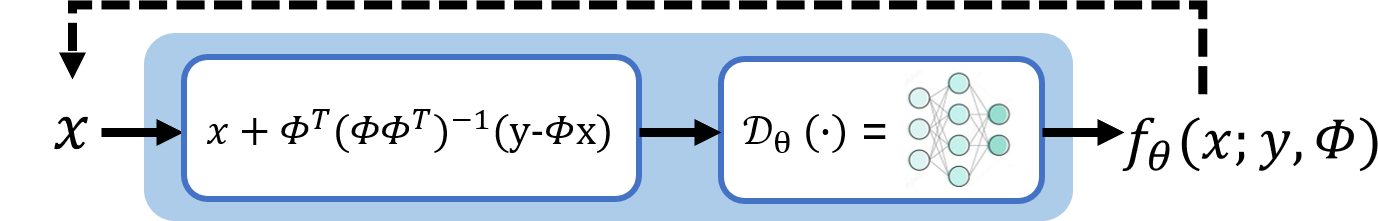
Figure 3.2: Illustration of our proposed DEQ for SCI using generalized alternating projection (GAP), i.e., DE-GAP.

3.2.3 Anderson Acceleration

To enforce fixed-point iterations converge more quickly, we make full use of the ability to accelerate inference with standard fixed-point accelerators, e.g., Anderson accelerator. Anderson acceleration utilizes previous iterations to seek promising directions to move forward. Under the setting of Anderson accelerator, we identify a vector $\bm{\alpha}^{(k)}\in\mathbb{R}^{s}$, for $\delta>0$:

$$\begin{aligned} \bm{x}^{(k+1)}=&\textstyle(1-\delta)\sum_{i=0}^{s-1}\mathbf{\bm{\alpha}}_{i}^{(k)}\bm{x}^{(k-i)}\\ &+\textstyle\delta\sum_{i=0}^{s-1}\mathbf{\bm{\alpha}}_{i}^{(k)}f_{\theta}(\bm{x}^{(k-i)};\bm{y},\bm{\Phi}),\end{aligned}$$ (3.7)

where the vector $\mathbf{\bm{\alpha}}_{i}^{(k)}$ is the solution to the optimization problem:

$$\textstyle\operatorname*{arg\,min}_{\mathbf{\bm{\alpha}}}||{\bf A}\bm{\alpha}||_{2}^{2},\quad s.t.\quad\mathbf{1}^{\top}\bm{\alpha}=1,$$ (3.8)

where ${\bf A}$ is a matrix whose $i$-th column is the vectorized residual $f_{\theta}(\bm{x}^{(k-i)};\bm{y},\bm{\Phi})-\bm{x}^{(k-i)}$, with $i=0,\dots,s-1$. When $s$ is small (e.g., $s=3$), the optimization problem in Eq. (3.8) introduces trivial computation.

3.3 Backward Pass

While previous work often utilizes Newton’s method to achieve the equilibrium and then backpropagate through all the Newton iterations, following Zhao et al., (2022); Gilton et al., (2021), we alternatively adopt another method with high efficiency and constant memory requirement.

3.3.1 Loss Function

To optimize network parameters $\theta$, stochastic gradient descent is used to minimize a loss function as follows:

$$\textstyle\theta^{*}=\operatorname*{arg\,min}_{\theta}\frac{1}{m}\sum_{i=1}^{m}\ell(f_{\theta}(\hat{\bm{x}}_{i};\bm{y}_{i},\bm{\Phi}_{i}),\bm{x}^{\star}_{i}),$$ (3.9)

where $m$ is the number of training samples; $\ell(\cdot,\cdot)$ is a given loss function, $\bm{x}^{\star}_{i}$ is the ground truth 3D data of the $i$-th training sample, $\bm{y}_{i}$ is the paired measurement, $\bm{\Phi}_{i}$ denotes the sensing matrix, and $f_{\theta}(\hat{\bm{x}}_{i};\bm{y}_{i},\bm{\Phi}_{i})$ denotes the reconstruction result given as the fixed point $\hat{\bm{x}}$ of the iteration map $f_{\theta}(\cdot\ ;\bm{y},\bm{\Phi})$, as derived from Eq. (3.2). The mean-squared error (MSE) loss is used for our video SCI reconstruction:

$$\textstyle\ell(\hat{\bm{x}},\bm{x}^{\star})=\frac{1}{2}||\hat{\bm{x}}-\bm{x}^{\star}||_{2}^{2}.$$ (3.10)

Since the reconstruction result is a fixed point of the iteration map $f_{\theta}(\cdot\ ;\bm{y},\bm{\Phi})$, gradient calculation of this loss term could be designed to avoid large memory demand. Following Gilton et al., (2021), we calculate the gradient of the loss term, which takes the network parameters $\theta$ into consideration.

3.3.2 Gradient Calculation

Following Zhao et al., (2022); Gilton et al., (2021), we calculate the loss gradient. Let $\ell$ be an abbreviation of $\ell(\hat{\bm{x}},\bm{x}^{\star})$ in Eq. (3.10), then the loss gradient is:

$$\begin{aligned} \textstyle\frac{\partial\ell}{\partial\theta}&={\left(\frac{\partial\hat{\bm{x}}}{\partial\theta}\right)}^{\top}\frac{\partial\ell}{\partial\hat{\bm{x}}}&={\left(\frac{\partial\hat{\bm{x}}}{\partial\theta}\right)}^{\top}{\left(\hat{\bm{x}}-\bm{x}^{\star}\right)},\end{aligned}$$ (3.11)

where $\frac{\partial\hat{\bm{x}}}{\partial\theta}$ is the Jacobian of $\hat{\bm{x}}$ evaluated at $\theta$, and $\frac{\partial\ell}{\partial\hat{\bm{x}}}$ is the gradient of $\ell$ evaluated at $\bm{x}^{\star}$.

Then to compute the Jacobian $\frac{\partial\hat{\bm{x}}}{\partial\theta}$, we recall the fixed point equation $\hat{\bm{x}}=f_{\theta}(\hat{\bm{x}};\bm{y},\bm{\Phi})$ in Eq. (3.2). By implicitly differentiating both sides of this fixed point equation, the Jacobian $\frac{\partial\hat{\bm{x}}}{\partial\theta}$ is solved as:

$$\textstyle\frac{\partial\hat{\bm{x}}}{\partial\theta}=\left[\bm{I}-\left.\frac{\partial f_{\theta}(\bm{x};\bm{y},\bm{\Phi})}{\partial\bm{x}}\right|_{\bm{x}=\hat{\bm{x}}}\right]^{-1}\frac{\partial f_{\theta}(\hat{\bm{x}};\bm{y},\bm{\Phi})}{\partial\theta},$$ (3.12)

which could be plugged into Eq. (3.11) and thus get:

$$\begin{aligned} \textstyle\frac{\partial\ell}{\partial\theta}=\left[\frac{\partial f_{\theta}(\hat{\bm{x}};\bm{y},\bm{\Phi})}{\partial\theta}\right]^{\top}\!{\left[\bm{I}-\left.\frac{\partial f_{\theta}(\bm{x};\bm{y},\bm{\Phi})}{\partial\bm{x}}\right|_{\bm{x}=\hat{\bm{x}}}\right]^{-\top}}{(\hat{\bm{x}}-\bm{x}^{\star})},\end{aligned}$$ (3.13)

where ^-⊤ denotes the inversion followed by transpose. As this method converted gradient calculation to the problem of calculating an inverse Jacobian-vector product, it avoids the backpropagation through many iterations of $f_{\theta}(\hat{\bm{x}};\bm{y},\bm{\Phi})$. To approximate the inverse Jacobian-vector product, we define the vector $\bm{a}^{(\infty)}$ as:

$$\textstyle\bm{a}^{(\infty)}={\left[\bm{I}-\left.\frac{\partial f_{\theta}(\bm{x};\bm{y},\bm{\Phi})}{\partial\bm{x}}\right|_{\bm{x}=\hat{\bm{x}}}\right]^{-\top}}\!{(\hat{\bm{x}}-\bm{x}^{\star})}.$$ (3.14)

Following Gilton et al., (2021), it is noted that $\bm{a}^{(\infty)}$ is a fixed point of the equation:

$$\begin{aligned} \bm{a}^{(k+1)}=\textstyle{\left[\left.\frac{\partial f_{\theta}(\bm{x};\bm{y},\bm{\Phi})}{\partial\bm{x}}\right|_{\bm{x}=\hat{\bm{x}}}\right]^{-\top}}\bm{a}^{(k)}+{(\hat{\bm{x}}-\bm{x}^{\star})},\\ \forall k=0,1,\dots,\infty.\end{aligned}$$ (3.15)

Therefore, the same algorithm used to calculate the fixed point $\hat{\bm{x}}$ could also be used to calculate $\bm{a}^{(\infty)}$ . The limit of fixed-point iterations for solving Eq. (3.15) with initial iterate $\bm{a}^{(0)}=\mathbf{0}$ is denoted equivalently to the Neumann series:

$$\bm{a}^{(\infty)}=\textstyle\sum_{p=0}^{\infty}\left\{{\left[\left.\frac{\partial f_{\theta}(\bm{x};\bm{y},\bm{\Phi})}{\partial\bm{x}}\right|_{\bm{x}=\hat{\bm{x}}}\right]^{\top}}\right\}^{p}\!{(\hat{\bm{x}}-\bm{x}^{\star})}.$$ (3.16)

To quickly calculate the vector-Jacobian products in Eq. (3.15) and Eq. (3.16), a lot of auto-differentiation tools (e.g., autograd packages in PytorchPaszke et al., (2019)) could be utilized. After the accurate approximation of $\bm{a}^{(\infty)}$ is calculated, the gradient in Eq. (3.11) is given by:

$$\textstyle\frac{\partial\ell}{\partial\theta}={\left(\frac{\partial f_{\theta}(\hat{\bm{x}};\bm{y},\bm{\Phi})}{\partial\theta}\right)}^{\top}\bm{a}^{(\infty)}.$$ (3.17)

3.4 Convergence Theory

Given the iteration map $f_{\theta}(\cdot\ ;\bm{y},\bm{\Phi}):{\mathbb{R}}^{nB}\rightarrow{\mathbb{R}}^{nB}$, in this section, we discuss conditions that guarantee the convergence of the proposed deep equilibrium models $\bm{x}^{(k+1)}=f_{\theta}(\bm{x}^{(k)};\bm{y},\bm{\Phi})$ to a fixed-point $\hat{\bm{x}}$ as $k\rightarrow\infty$.

(Convergence of DE-RNN). For all $\bm{x},\bm{x}^{\prime}\in{\mathbb{R}}^{nB}$, if there exists a constant $0\leq c<1$ satisfies that:

$$\|{\rm RNN}_{\theta}(\bm{x},\bm{y},\bm{\Phi})-{\rm RNN}_{\theta}(\bm{x}^{\prime},\bm{y},\bm{\Phi})\|\leq c\|\bm{x}-\bm{x}^{\prime}\|,$$ (3.18)

then the DE-RNN iteration map $f_{\theta}(\bm{x};\bm{y},\bm{\Phi})$ is contractive.

(Convergence of DE-GAP). For all $\bm{x},\bm{x}^{\prime}\in{\mathbb{R}}^{nB}$, if there exists a $\varepsilon>0$ such that the denoiser $\mathcal{D_{\theta}}:{\mathbb{R}}^{nB}\rightarrow{\mathbb{R}}^{nB}$ satisfies:

$$\|(\mathcal{D}_{\theta}-{\bf I})(\bm{x})-(\mathcal{D}_{\theta}-{\bf I})(\bm{x}^{\prime})\|\leq\varepsilon||\bm{x}-\bm{x}^{\prime}||,$$ (3.19)

where $(\mathcal{D}_{\theta}-{\bf I})(\bm{x}):=\mathcal{D}_{\theta}(\bm{x})-\bm{x}$, that is, we assume the map $\mathcal{D}_{\theta}-{\bf I}$ is $\varepsilon$-Lipschitz, then the DE-GAP iteration map $f_{\theta}(\cdot;\bm{y},\bm{\Phi})$ defined in Eq. (3.6) satisfies:

$$\textstyle\|f_{\theta}(\bm{x};\bm{y},\bm{\Phi})-f_{\theta}(\bm{x}^{\prime};\bm{y},\bm{\Phi})\|\leq\eta\|\bm{x}-\bm{x}^{\prime}\|$$ (3.20)

for all $\bm{x},\bm{x}^{\prime}\in{\mathbb{R}}^{nB}$. The coefficient $\eta$ is less than 1, in which case the DE-GAP iteration map $f_{\theta}(\bm{x};\bm{y},\bm{\Phi})$ is contractive.

Following Gilton et al., (2021), to prove $f_{\theta}(\cdot;\bm{y},\bm{\Phi})$ is contractive it suffices to show $||\partial_{\bm{x}}f_{\theta}(\bm{x};\bm{y},\bm{\Phi})||<1$ for all $\bm{x}\in{\mathbb{R}}^{nB}$, where $||\cdot||$ denotes the spectral norm, $\partial_{\bm{x}}f_{\theta}(\bm{x};\bm{y},\bm{\Phi})$ is the Jacobian of $f_{\theta}(\bm{x};\bm{y},\bm{\Phi})$ with respect to $\bm{x}\in{\mathbb{R}}^{nB}$ given by:

$$\partial_{\bm{x}}f_{\theta}(\bm{x};\bm{y},\bm{\Phi}) =\partial_{\bm{x}}\mathcal{D_{\theta}}(\bm{x})({\bf I}-{\bm{\Phi}}^{\top}(\bm{\Phi}{\bm{\Phi}}^{\top})^{-1}\bm{\Phi}),$$ (3.21)

where $\partial_{\bm{x}}\mathcal{D_{\theta}}\in{\mathbb{R}}^{nB\times nB}$ is the Jacobian of $\mathcal{D_{\theta}}:{\mathbb{R}}^{nB}\rightarrow{\mathbb{R}}^{nB}$ with respect to $\bm{x}\in{\mathbb{R}}^{nB}$.

Finally, we derive (details can be found in Zhao, (2022) or supplementary material):

$$\begin{aligned} ||\partial_{\bm{x}}f_{\theta}(\bm{x};\bm{y},\bm{\Phi})||=&\ ||\partial_{\bm{x}}\mathcal{D_{\theta}}(\bm{x})({\bf I}-\bm{\Psi})||,\\ =&\ ||\partial_{\bm{x}}\mathcal{D_{\theta}}(\bm{x})-\partial_{\bm{x}}\mathcal{D_{\theta}}(\bm{x})\bm{\Psi}||\\ =&\ ||\partial_{\bm{x}}\mathcal{D_{\theta}}(\bm{x})-{\bf I}+{\bf I}-\partial_{\bm{x}}\mathcal{D_{\theta}}(\bm{x})\bm{\Psi}||\\ \leq&\ ||\partial_{\bm{x}}\mathcal{D_{\theta}}(\bm{x})-{\bf I}||+||{\bf I}-\partial_{\bm{x}}\mathcal{D_{\theta}}(\bm{x})\bm{\Psi}||\\ \leq&\ \varepsilon+1+||(\partial_{\bm{x}}\mathcal{D_{\theta}}(\bm{x})-{\bf I}+{\bf I})\bm{\Psi}||\\ =&\ 1+\varepsilon+||(\partial_{\bm{x}}\mathcal{D_{\theta}}(\bm{x})-{\bf I})\bm{\Psi}+\bm{\Psi}||\\ \leq&\ 1+\varepsilon+||(\partial_{\bm{x}}\mathcal{D_{\theta}}(\bm{x})-{\bf I})\bm{\Psi}||+||\bm{\Psi}||\\ \leq&\ 1+\varepsilon+\varepsilon||\bm{\Psi}||+||\bm{\Psi}||\\ =&\ (1+\varepsilon)(1+||\bm{\Psi}||)\\ \leq&\textstyle(1+\varepsilon)\max_{i}|1-\lambda_{i}|,\end{aligned}$$ (3.22)

where $\lambda_{i}$ are eigenvalues of ${\bm{\Phi}}^{\top}(\bm{\Phi}{\bm{\Phi}}^{\top})^{-1}\bm{\Phi}$; and the inequality Eq. (3.22) is based on the assumption that the map $(\mathcal{D}_{\theta}-{\bf I})(\bm{x}):=\mathcal{D}_{\theta}(\bm{x})-\bm{x}$ is $\varepsilon$-Lipschitz. Therefore the spectral norm of its Jacobian $\partial_{\bm{x}}\mathcal{D_{\theta}}(\bm{x})-{\bf I}$ is bounded by $\eta$, which demonstrates $f_{\theta}$ is $\eta$-Lipschitz with $\eta=(1+\varepsilon)\max_{i}|1-\lambda_{i}|$.

It is worth noting that convergence is not yet guaranteed in our calculation above since $\eta$ is larger than 1. In SCI cases, it is challenging to provide a theoretical guarantee. However, we observe our models converge well in the experiments.

References

- Bai et al., (2019) Bai, S., Kolter, J. Z., and Koltun, V. (2019). Deep equilibrium models. arXiv preprint arXiv:1909.01377.
- Cheng et al., (2022) Cheng, Z., Chen, B., Lu, R., Wang, Z., Zhang, H., Meng, Z., and Yuan, X. (2022). Recurrent neural networks for snapshot compressive imaging. IEEE Transactions on Pattern Analysis and Machine Intelligence.
- Gilton et al., (2021) Gilton, D., Ongie, G., and Willett, R. (2021). Deep equilibrium architectures for inverse problems in imaging. arXiv preprint arXiv:2102.07944.
- Liu et al., (2018) Liu, Y., Yuan, X., Suo, J., Brady, D. J., and Dai, Q. (2018). Rank minimization for snapshot compressive imaging. IEEE transactions on pattern analysis and machine intelligence, 41(12):2990–3006.
- Meng et al., (2020) Meng, Z., Jalali, S., and Yuan, X. (2020). Gap-net for snapshot compressive imaging. arXiv preprint arXiv:2012.08364.
- Meng and Yuan, (2021) Meng, Z. and Yuan, X. (2021). Perception inspired deep neural networks for spectral snapshot compressive imaging. In 2021 IEEE International Conference on Image Processing (ICIP), pages 2813–2817. IEEE.
- Paszke et al., (2019) Paszke, A., Gross, S., Massa, F., Lerer, A., Bradbury, J., Chanan, G., Killeen, T., Lin, Z., Gimelshein, N., Antiga, L., et al. (2019). Pytorch: An imperative style, high-performance deep learning library. Advances in neural information processing systems, 32:8026–8037.
- Qiao et al., (2020) Qiao, M., Meng, Z., Ma, J., and Yuan, X. (2020). Deep learning for video compressive sensing. APL Photonics, 5(3):030801.
- Walker and Ni, (2011) Walker, H. F. and Ni, P. (2011). Anderson acceleration for fixed-point iterations. SIAM Journal on Numerical Analysis, 49(4):1715–1735.
- Wang et al., (2022) Wang, L., Cao, M., Zhong, Y., and Yuan, X. (2022). Spatial-temporal transformer for video snapshot compressive imaging. arXiv preprint arXiv:2209.01578.
- Wu et al., (2022) Wu, Z., Yang, C., Su, X., and Yuan, X. (2022). Adaptive deep pnp algorithm for video snapshot compressive imaging. arXiv preprint arXiv:2201.05483.
- Wu et al., (2021) Wu, Z., Zhang, J., and Mou, C. (2021). Dense deep unfolding network with 3d-cnn prior for snapshot compressive imaging. arXiv preprint arXiv:2109.06548.
- Yang et al., (2015) Yang, J., Liao, X., Yuan, X., Llull, P., Brady, D. J., Sapiro, G., and Carin, L. (2015). Compressive sensing by learning a Gaussian mixture model from measurements. IEEE Transaction on Image Processing, 24(1):106–119.
- Yang et al., (2014) Yang, J., Yuan, X., Liao, X., Llull, P., Sapiro, G., Brady, D. J., and Carin, L. (2014). Video compressive sensing using Gaussian mixture models. IEEE Transaction on Image Processing, 23(11):4863–4878.
- Yang and Zhao, (2022) Yang, Q. and Zhao, Y. (2022). Revisit dictionary learning for video compressive sensing under the plug-and-play framework. In Seventh Asia Pacific Conference on Optics Manufacture and 2021 International Forum of Young Scientists on Advanced Optical Manufacturing (APCOM and YSAOM 2021), volume 12166, pages 2018–2025. SPIE.
- Yuan, (2016) Yuan, X. (2016). Generalized alternating projection based total variation minimization for compressive sensing. In 2016 IEEE International Conference on Image Processing (ICIP), pages 2539–2543. IEEE.
- Yuan et al., (2020) Yuan, X., Liu, Y., Suo, J., and Dai, Q. (2020). Plug-and-play algorithms for large-scale snapshot compressive imaging. In IEEE/CVF Conference on Computer Vision and Pattern Recognition (CVPR).
- Yuan et al., (2021) Yuan, X., Liu, Y., Suo, J., Durand, F., and Dai, Q. (2021). Plug-and-play algorithms for video snapshot compressive imaging. IEEE Transactions on Pattern Analysis and Machine Intelligence, pages 1–1.
- Zhao, (2022) Zhao, Y. (2022). Mathematical cookbook for snapshot compressive imaging. arXiv preprint arXiv:2202.07437.
- Zhao et al., (2022) Zhao, Y., Zheng, S., and Yuan, X. (2022). Deep equilibrium models for video snapshot compressive imaging. arXiv preprint arXiv:2201.06931.
- Zheng et al., (2021) Zheng, S., Wang, C., Yuan, X., and Xin, H. L. (2021). Super-compression of large electron microscopy time series by deep compressive sensing learning. Patterns, 2(7):100292.