A precortical module for robust CNNs to light variations

Abstract

We present a simple mathematical model for the mammalian low visual pathway, taking into account its key elements: retina, lateral geniculate nucleus (LGN), primary visual cortex (V1). The analogies between the cortical level of the visual system and the structure of popular CNNs, used in image classification tasks, suggests the introduction of an additional preliminary convolutional module inspired to precortical neuronal circuits to improve robustness with respect to global light intensity and contrast variations in the input images. We validate our hypothesis on the popular databases MNIST, FashionMNIST and SVHN, obtaining significantly more robust CNNs with respect to these variations, once such extra module is added.

A precortical module for robust CNNs

to light variations

R. Fioresi, J. Petkovic

1 Introduction

The fascinating similarities between CNN architectures and the modeling of the mammalian low visual pathway are a current active object of investigation (see [31], [6], [12] and refs. therein). Historically, the study of border and visual perception started around 1920’s with the Gestalt psychology formalization (Prägnanz laws) of the perception (lines, colors and contours, see [26] and refs. therein). Then, the foundational work [19] introduced a more scientific approach to the subject, defining the concept of receptive field, simple and complex cells, together with an anatomically sound description of the visual cortex in mammals.

This study paved the way to the mathematical modeling for such structures. In particular special attention was given to the primary visual cortex V1 (see [41]), whose orientation sensitive simple cells, together with the complex and hypercomplex cells, inspired the modeling of algorithms [32] contibuting to the spectacular success of Deep Learning CNNs [24]. With a more geometric approach in [7], the introduction on V1 of a natural subriemannian metric [20, 17], following the seminal work [30], led to interesting interpretations of the border completion mechanism.

While the mathematical modeling became more sophisticated (see [34] and refs therein), the insight into the physiological functioning of the visual pathway led to more effective algorithms in image analysis [15, 6]. In particular, the Cartan geometric point of view on the V1 modeling [34], fueled new interest and suggests a physiological counterpart for the new algorithms based on group equivariance in geometric deep learning approaches (see [5, 9] and refs therein).

The purpose of our paper is to provide a simple mathematical model for the low visual pathway, comprehending the retina, the lateral geniculate nucleus (LGN) and the primary visual cortex (V1) and to use such model to construct a preliminary convolutional module, that we call precortical to enhance the robustness of popular CNNs for image classification tasks. We want the CNN to gain the outstanding ability of the human eye to react to large variations in global light intensity and contrast. This can be achieved by mimicking the gain tuning effect implemented the precortical portion of the mammalian visual pathway. This effect consists in the following: since the low visual circuit needs to respond to a vast range of light stimuli, that spans over $10$ orders of magnitude, it is equipped with a lateral inhibition mechanism which allows a low latency and a high sensitivity response. This mechanism is functionally embedded in the center-surround receptive fields of retinal bipolar cells, retinal ganglions and LGN neurons and is able to achieve both border enhancing and decorrelation between the perceived light intensity in single pixels and the mean light value in a given image [21]. We will show that, if in the early levels of a CNN such receptive fields are learned in the form of convolutional filters, there is a considerable improvement in accuracy, when considering dimmed light or low contrast examples, i.e. examples not belonging to the statistic of the training set.

The organization of this paper is as follows. We start with a simple mathematical formalization of the low visual pathway, which accounts for its key components. Though this material is not novel, we believe our terse presentation can greatly help to elucidate the relation between mathematical entities, like bundles or vector fields and the local physiological structure of retina and V1, together with their functioning.

The similarities between the inner structure of CNNs and the physiological visual perception mechanism, once appropriately mathematically modeled as above, show that popular CNNs structure, for image classification tasks, do not take into full consideration the role of the precortical structures, which are responsible for a correct adjustment to global light intensity and contrast in an image. Our observations then, suggest the introduction of a precortical module (see also [31, 6]), which mimics the functioning of retina and LGN cells and reacts appropriately to the variations of the light intensity and the contrast. Once such module is introduced, we verify in our experiments on the MNIST, FashionMNIST and SVHM databases that our CNN shows robustness with respect to such large variations. So effectively our experiments and subsequent implementations show the importance of the module introduced in [6].

The impact and potential of our approach is that a new simplified, but accurate, mathematical modeling of the low visual pathway, can lead to key cues on algorithm design, which add robustness and allow high performances beyond the type of data the algorithm is trained with, exactly as it happens for the human visual perception. In a forthcoming research, we plan to further explore this study by analyzing the autoencoder performances in the border completion, using the mathematical description via subriemannian metric geodesic.

2 Related work

The structure of the mammalian visual pathway was extensively explored in the last century both from an anatomical and a functional point of view (see [11] and [21] and refs therein). New aspects, however, are still discovered nowadays at each level of its structure: from new cellular types [33] to new functional circuits [22], shedding more light on the formal process of visual information encoding (see [36], [40], [37]). The striking correspondence between the training of mammals visual system and popular CNN training was elucidated in [1], suggesting more exploration into this direction is necessary. Similarities between deep CNN structure and the human visual pathway have been then increasingly explored in this framework. From the first appearance of the neocognitron [16], the feature extracting action of the convolutional module has been widely adopted to tackle a number of visual tasks, developing models which presented striking analogies with mammalian cellular subtypes and their receptive fields [24, 18, 6, 31]. These similarities were studied, in particular, in relation to the deeper components of the visual pathway, starting from the hypercolumnar structure of the primary visual cortex V1 and continuing with superior processing centers, like V4 and the inferior temporal cortex ([27] and the references therein). The exploration of similarities with the first stages of visual perception and in particular to the receptive field structure of retinal and geniculate units or with their precise regularizing effect on the perceived image appears also in [13], [10], [14], [42]. Another recent attempt in this direction is also in [6], where a biologically inspired CNN is studied in connection with the Retinex model [23], elucidated mathematically in [35] and then implemented [28] (see also refs. therein). Also in [29] and more recently in [39], [4] appear some observations the behaviour of artifician neurons on contrast and more generally robustness.

3 The visual pathway

The visual pathway consists schematically of the following structures: the eye, the optic nerve, the lateral geniculates nucleus (LGN), the optic radiation and the primary visual cortex (V1). In our discussion, we focus only on the retina, LGN and V1, because these are the parts in which the processing of the signal (i.e. the images) requires a more articulate modeling.

The retina consists of photoreceptor cells, called receptors, which measure the intensity of light. We model part of the retina, the hemiretinal receptoral layer, with a compact simply connected domain $E$ in $\mathbb{R}^{2}$. We take a portion and not the whole retina, because we want to avoid to cross the median cleft line in the visual field, which is interpreted and processed in a more complex way (see [2]).

We define then a receptorial activation field as a function

$$\begin{array}[]{cccc}{\mathcal{R}}:&E&\longrightarrow&\mathbb{R}\\ &(x,y)&\mapsto&{\mathcal{R}}(x,y)\end{array}$$ (1)

associating to each point $(x,y)$, corresponding to a receptor in the retina, an activation rate given by the scalar ${\mathcal{R}}(x,y)$. We do not assume ${\mathcal{R}}$ to be continuous, however, by its physiological significance, it will be bounded.

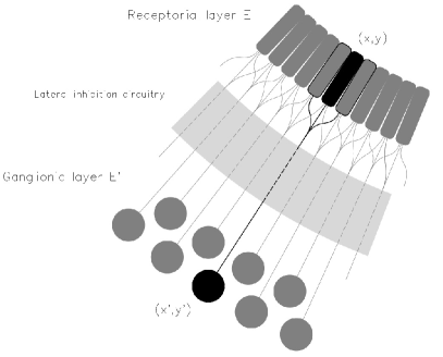
Figure 1: Schematic structure of receptorial and ganglionic layers in retina

We may then interpret ${\mathcal{R}}$ as coming from an image in the visual field. We will not distinguish between on and off receptors, as their final effect on the downstream neurons is the same from a logical point of view. We assume ${\mathcal{R}}(x,y)$ to be proportional to the intensity of the light falling on $(x,y)$. The ganglionic layer $\widetilde{E}$ (see Fig. 1) sits a few layers down the visual pathway.

To each receptor $(x,y)$ in $E$ there is a corresponding ganglion $(x^{\prime},y^{\prime})$ in $\widetilde{E}$ with its receptive field centered in $(x^{\prime},y^{\prime})$ so that we have a natural distance preserving identification between $E$ and $\widetilde{E}$, given by an isometry $G:E\longrightarrow\widetilde{E}$.

The ganglionic activation pattern, however, is quite different from the hemiretinal receptors one (1):

$$\widetilde{{\mathcal{R}}}:\widetilde{E}\longrightarrow\mathbb{R},\quad\widetilde{{\mathcal{R}}}(x^{\prime},y^{\prime})=\int_{U_{\rho}(x,y)}\mathcal{K}(u,v){\mathcal{R}}(u,v)\,du\,dv\quad\hbox{with}\quad G(x,y)=(x^{\prime},y^{\prime})$$ (2)

where

$$U_{\rho}(x,y)=\big{\{}(u,v)\in\mathbb{R}^{2}:(u-x)^{2}+(v-y)^{2}\leq\rho^{2}\big{\}},$$

$$\mathcal{K}(x,y)=\begin{cases}\pm 1&\mathrm{if}\quad(u-x)^{2}+(v-y)^{2}\leq(\rho-\epsilon)^{2}\\ \\ \mp 1&\mathrm{if}\quad(\rho-\epsilon)^{2}<(u-x)^{2}+(v-y)^{2}\leq\rho^{2}\end{cases}$$

The identification between $E$ and $\widetilde{E}$ given by $G$ is not a manifold morphism: in fact the correspondence between functions follows (4), which is an integral transform with kernel $\mathcal{K}(x,y)$. This models effectively the mechanism of firing of hemiretinal receptors: for each activation disc we always have an inhibition crown around it. This is the key mechanism, responsible for the border and contrast enhancement, that we shall implement with our precortical module in Sec. 5.

We notice an important consequence, whose proof is in App. A, to ease the reading.

Proposition 3.1.

The hemiretinal ganglionic activation field $\widetilde{{\mathcal{R}}}$ is Lipschitz continuous in both variables on $\widetilde{E}$.

This proposition encodes the fact that the visual system is able to reconstruct a border percept also for non continuous images. This fact was already noticed in [30], where edge interruptions are taken into account and defined as cusps or elementary catastrophes. We illustrate this phenomenon in Fig. 2, which is perceived as a unitary curvilinear shape with clear borders, though composed of isolated black dots. There is indeed a further smoothing reconstruction carried out in the LGN, so that our image will provide us with a smooth function in place of $\widetilde{{\mathcal{R}}}$, [8]. We shall not describe such modeling for the present work.

We now come to the last portion of the visual pathway: the primary visual hemicortex, that we shall still denote with $V1$. The retinotopic map is a distance preserving homeomorphism between the hemiretinal receptorial layer and the primary visual hemicortex (see [2] for a concrete realization). We can therefore identify $V1$ with a compact domain $V$ in $\mathbb{R}^{2}$.

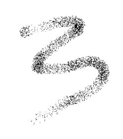
Figure 2: Border percepts for a non continuous image

The pointwise identification, however, is not sufficient to model the behaviour of $V1$. In fact for each point of the visual cortex we have three main information to take into account:

1. The absolute position of the corresponding point in the retina, which receives a stimulus;

2. the orientation $\theta$ of some perceived edge through the point (simple and complex cells);

3. the curvature $k$ of some perceived edge through the point (hypercomplex cells).

While the first feature is encoded by the points in the domain $V$, additional modelization is needed for the construction of orientation and curvature information. For this reason, a point in $V1$ is identified with a biological structure, called hypercolumn, which contains a plethora of cell families, each analyzing a specific aspect of the visual information. We assume that at each point of $V1$ is present a full set of simple, complex and hypercomplex orientation columns (a so called full orientation hypercolumn).

We briefly recap the various types of cells in $V1$, since their behaviour plays a key role in our modeling.

• Simple cells: they exhibit a rich and multifaceted behavioural pattern in response to positional, orientational and dynamic features of a light input. Traditionally, for their modeling is used the asymmetrical part of a Gabor filter, though in recent works more importance is given to the role of the LGN and the actual neuroanatomical structure (see [25, 3]).

• Complex cells: they receive input directly from simple cells (see [19]) and they show a linear response depending on the orientation of some static stimulus over a certain receptive field. It is important to note that this response is invariant under a $180^{0}$ rotation of the stimulus.

• Hypercomplex cells: they are also called end-stopped cells and they are maximally activated by oriented stimuli positioned in the central region of their receptive field. They are maximally inhibited by peripheric stimuli with the same orientation. Such cells are therefore not particularly reactive to long straight lines, firing briskly if perceiving curves or corners.

As we shall see in our next section, in order to take into account all different cells behaviours in the hypercolumn, we need to model $V1$ using the mathematical concept of fiber bundle.

4 The Primary Visual Cortex

We want to provide a mathematical description of V1, starting from the actual neuroanatomical structures and taking into account the combined effects of complex and simple cells. Though this material is mostly known (see [20, 17, 7, 41]), our novel and simplified presentation will elucidate the role of the key components of the visual pathway, while keeping a faithful representation of the neuroanatomical structures.

Let $D\subset\mathbb{R}^{2}$ be compact, simply connected. We start by defining the orientation of a function $F:D\longrightarrow\mathbb{R}$; it will be instrumental for our modelization of $V1$. On the manifold $D\times S^{1}$ define the vector field $Z$:

$$Z(x,y,\theta)=-\sin\theta\;\partial_{x}+\cos\theta\;\partial_{y}$$

where as usual $\partial_{x}$, $\partial_{y}$ form a basis for the tangent space of $\mathbb{R}^{2}$ at each point and $\theta$ is the coordinate for $S^{1}$. To ease the notation we drop $x,y$ in the expression of $Z$, writing $Z(\theta)$ in place of $Z(x,y,\theta)$.

Definition 4.1.

Let $D\subset\mathbb{R}^{2}$ be compact and simply connected and $F:D\longrightarrow\mathbb{R}$ a smooth function. Let $\mathrm{reg}(D)\subset D$ be the subset of regular points of $F$ (i.e. $p\in D$, $dF(p)\neq(0,0)$). We define the orientation of $F$ as:

$$\begin{array}[]{ccccc}\Theta:&\mathrm{reg}(E^{\prime})&\longrightarrow&S^{1}&\\ &(x,y)&\longmapsto&\Theta(x,y)&:=\mathrm{argmax}_{\theta\in S^{1}}{\bigl{\{}Z(\theta)F(x,y)\bigr{\}}}\end{array}$$ (3)

The map $\Theta$ is well defined because of the following proposition.

Proposition 4.2.

Let $F:D\longrightarrow\mathbb{R}$ as above and $(x_{0},y_{0})\in D$ a regular point for $F$. Then, we have the following:

1. There there exists a unique $\theta_{x_{0},y_{0}}\in S^{1}$ for which the function $\zeta_{x,y}:S^{1}\longrightarrow\mathbb{R}$, $\zeta_{x,y}(\theta):=Z(\theta)\,F(x,y)$ attains its maximum.

2. The map $\Theta:\mathrm{reg}(D)\longrightarrow S^{1}$, $\Theta(x,y)=\theta_{x,y}$ is well defined and differentiable.

3. The set:

   $$\Phi=\{(x,y,\Theta(x,y))\in D\times S^{1}:\Theta(x,y)=\theta_{x,y}\}$$

   is a regular submanifold of $D\times S^{1}$.

Proof.

(1). Since $\zeta_{x,y}$ is a differentiable function on a compact domain it admits maximum, we need to show it is unique. We can explicitly express:

$$\zeta_{x,y}(\theta)=-\sin\theta\;\partial_{x}F+\cos\theta\;\partial_{y}F$$

Since $(\partial_{x}F,\partial_{y}F)\neq(0,0)$ and it is constant, by elementary considerations, taking the derivative of $\zeta_{x,y}$ with respect to $\theta$ we see the maximum is unique.

(2). $\Theta$ is well defined by $(1)$ and differentiable.

(3). It is an immediate consequence of the implicit function theorem.

∎

Notice the following important facts:

• the locality of the operator $Z(\theta)$ mirrors the locality of the hypercolumnar anatomical connections;

• its operating principle is a good description of the combined action of simple and complex cells (though different from their individual behaviour);

We now look at an example given by Fig. 3 of the behaviour of $Z$ on an image, that we view as a function $F:D\longrightarrow\mathbb{R}$.

Here $D\cong\widetilde{E}$, that is $F$ is a hemiretinal ganglionic receptive field.

We can see in our example that for each point $(x,y)$ near the border of the dark circle represented by the image $F$, there exists a value $\theta(x,y)$ for which the function $Z(\theta)F(x,y)$ is maximal (we color in white the maximum, in black the minimum). This value is indeed the angle between the tangent line to a visually perceived orientation in $(x,y)$ and the $x$ axis.

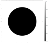
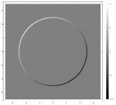
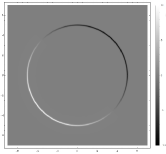
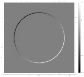
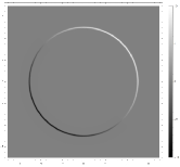
Figure 3: Graphs of $F(x,y)=-\frac{1}{1+(0.04\,x^{2}+0.04\,y^{2})^{100}}$, $Z(\frac{\pi}{4})F$, $Z(\frac{3\pi}{4})F$, $Z(\frac{7\pi}{4})F$ and $Z(\frac{5\pi}{4})F$.

Since in $V1$ at each point we need to consider all possible orientations, coming from different receptive fields, following [20, 17, 41], we model $V1$ as the fiber bundle $\mathcal{E}:=V\times S^{1}\longrightarrow V$, that we call the orientation bundle. Notice that $V$ is a domain $D\subset\mathbb{R}^{2}$ and naturally identified with $\widetilde{E}$ and $E$ with a distance preserving homeomorphism. Then, each ganglionic receptive field $\widetilde{{\mathcal{R}}}$, after LNG smoothing will give us a smooth section $\Theta$ of $\mathcal{E}$, through the identification we detailed above and elucidated in our example.

5 Experiments

We now take into exam a popular CNN: LeNet 5 and, based on the analogies with the low visual pathway elucidated in our previous discussion, we modify it by introducing a precortical module.

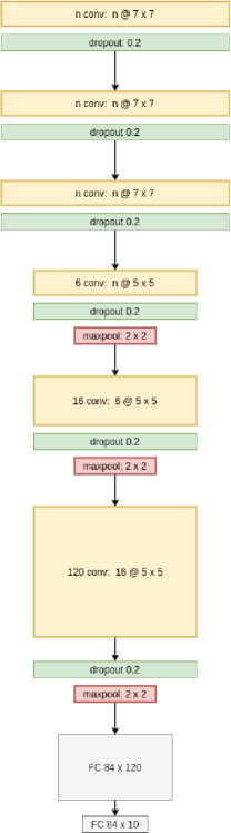
Figure 4: RetiLeNet structure; n = image color channels

The LeNet 5 convolutional layers have surprisingly strong similarities with the cortical directional hypercolumns: the stacked organization of the layers closely resembles the feed forward structure of the simple - complex - hypercomplex cell path (see Sec. 4). Also, the weights of the first convolutional layer converge to an integral kernel (see eq. (4)), which makes it sensitive to directional feature extraction. To allow the emergence of the precortical gain tuning effect (see Sec. 1), we structured our model as follows. We insert at the beginning the precortical module consisting of a sequence of convolutional, dropout and hyperbolic tangent activation layer, repeated three times. This number was chosen according to [11] and corresponds to the three vertical types of cells present in the precortical portion of the visual path (bipolar cell, retinal ganglion, LGN neuron). The number of features in each convolutional layer was chosen equal to the number of color channels (one for MNIST and FashionMNIST, three for SVHN) and the padding was set to (kernel_size-1)/2 to preserve the dimension of the input data. The output of this module, denominated precortical module was then fed to a slightly modified version of LeNet 5 (Fig. 4). The number kernel_size is taken as an hyperparameter and chosen for each dataset, according to the best performance. Finally, a modified LeNet 5 without the precortical module was trained on the same datasets and used for accuracy comparison. The training for both CNNs, that we denote RetiLeNet and LeNet 5 (with and without the precortical module), was carried out without any image preprocessing or data augmentation using the ADAM optimizer, with learning rate $0.001$ and a batch size of 128.
Since we want to study the effect on robustness of the precortical module, we tested the two models on transformed test sets. In particular, we considered the two transformations:

1. Mean offset (luminosity change): each pixel $x_{i}$ of the input image $X$ was shifted by an offset value $\mu$ as

   $$x_{i}\leftarrow x_{i}-\mu$$

   From a phenomenological point of view this represents a variation in the global light intensity.

2. Distribution scaling (contrast change): each pixel $x_{i}$ of a given image is modified with a deviation parameter $\sigma$ as

   $$x_{i}\leftarrow\frac{x_{i}-\bar{X}}{\sigma}+\bar{X}$$

   with $\bar{X}$ the mean pixel value in the image. In this fashion we obtain a modification in the image contrast.

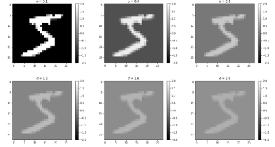
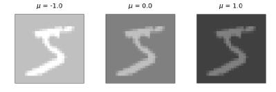
Figure 5: New samples generated by contrast reduction via $\sigma$ (left) and light dimming via $\mu$ (right).

5.1 Results

After training both models LeNet 5 and RetiLeNet (LeNet 5 with the precortical module) on MNIST, FashionMNIST and SVHN, choosing the hyperparameter kernel_size equal to 7 for RetiLeNet, we observe that in general, RetiLeNet performed better than LeNet 5 on the three datasets, as shown in Table 1. We also notice that the addition of the precortical module did not impact greatly on the final accuracy for the unmodified datasets, that is taking $\mu=0$, $\sigma=1$, accounting for a slight score improvement on SVHN and, surprisingly, a slight worsening on MNIST and FashionMNIST (see 1).

	$\mu$			$\sigma$
MNIST	-2.0	0	1.0	0.1	1.0	3.9
LeNet 5	0.120	0.991	0.119	0.915	0.991	0.485
RetiLeNet 5	0.097	0.988	0.787	0.984	0.988	0.907
	$\mu$			$\sigma$
FashionMNIST	-2.0	0	2.0	0.1	1.0	3.9
Lenet 5	0.168	0.887	0.100	0.836	0.887	0.422
Mod Lenet 5	0.770	0.880	0.781	0.805	0.880	0.806
	$\mu$			$\sigma$
SVHN	-2.0	0	2.0	0.1	1.0	3.9
Lenet 5	0.806	0.868	0.006	0.723	0.868	0.776
Mod Lenet 5	0.831	0.886	0.738	0.849	0.886	0.832

Table 1: Accuracies achieved with and without the precortical module versus $\mu$ and $\sigma$ sweeps. Notice: for MNIST the highest $\mu$ reported is 1.0 while it is 0.2 for the other two datasets.

We notice a better performance of RetiLeNet , with respect to LeNet 5 , on the transformed dataset, that is when we modify the contrast (via $\sigma$) and the light intensity (via $\mu$), see Fig. 6, 7, 8. The improvement in performance is particularly noticeable in the case of low contrast ($\sigma$ = 3.9) and very dark examples ($\mu$ = 2 for SVHN and FashionMNIST, $\mu$=1 for MNIST), where the accuracy of RetiLeNet is consistently greater than 75% in comparison with LeNet 5 accuracies, which are far lower. The reason for this behaviour is the strong stabilizing effect that the first (convolutional) layer of the precortical module has on the input image, in the analogy to the modeling for the receptive fields introduced in (4).

To elucidate this stabilizing effect, we choose an example from each dataset and look at the corresponding first hidden output, while the parameters $\mu$ and $\sigma$ vary (see Fig. 9, 10, 11). As far as the $\mu$ shift is concerned we see that this effect is very evident: for large variations of $\mu$ we have a pixel average close to zero after the first convolutional layer. In particular, we notice a correlation between a worse stabilizing action and a worse model performance, by comparing what happens with MNIST with respect to FashionMNIST and SVHN. Despite the small number of datasets considered, we think it may hint to a significant phenomenon worth a further investigation.

Moreover, we can see close similarities between this effect and the actual biological lateral inhibition phenomenon emerging at the bipolar cell level in the retina corresponding indeed to the first of our precortical convolutional layers. This biological phenomenon is responsible for the gain adjustment and border enhancement mechanisms which allow the visual system to respond correctly to strong changes in ambient light conditions.

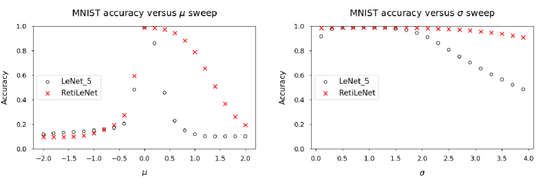
Figure 6: Accuracy for $\mu$, $\sigma$ variations in MNIST

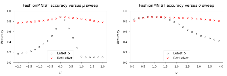
Figure 7: Accuracy for $\mu$, $\sigma$ variations in FashionMNIST

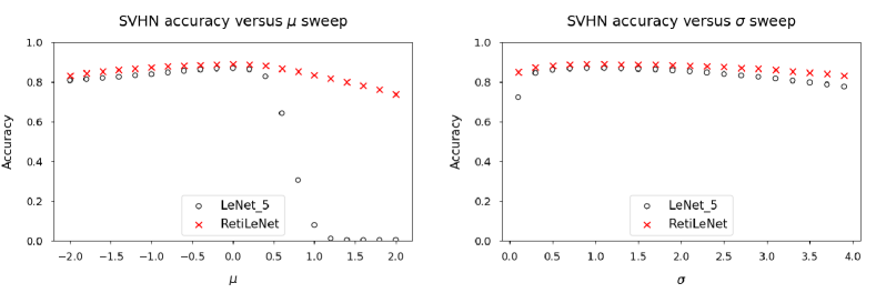
Figure 8: Accuracy for $\mu$, $\sigma$ variations in SVHN

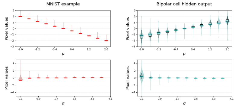
Figure 9: Pixel value distributions before (red) and after (green) first precortical convolutional layer for $\mu$, $\sigma$ variations in MNIST. (whiskers 1.5, violin kernel bandwidth 1.06)

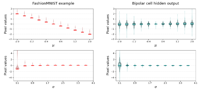
Figure 10: Pixel value distributions before (red) and after (green) first precortical convolutional layer for $\mu$, $\sigma$ variations in FashionMNIST. (whiskers 1.5, violin kernel bandwidth 1.06)

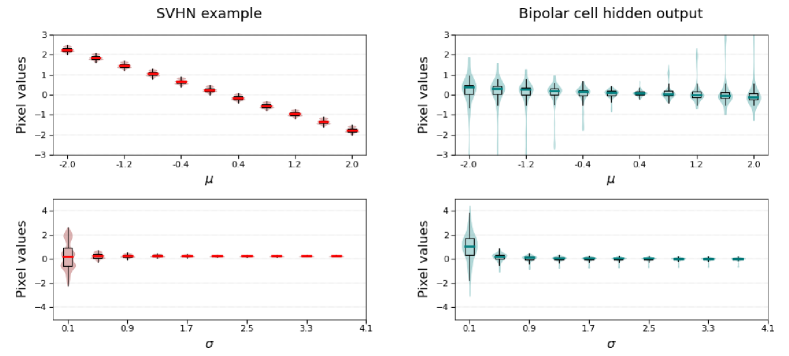
Figure 11: Pixel value distributions before (red) and after (green) first precortical convolutional layer for $\mu$, $\sigma$ variations in SVHN. (whiskers 1.5, violin kernel bandwidth 1.06)

6 Conclusions

Our simple mathematical model of the low visual pathway of mammals retains the descriptive accuracy of more complicated models and it is better suited to elucidate the similarities between visual physiological structures and CNNs. The precortical neuronal module, inspired by our mathematical modeling, when added to a popular CNN (LeNet 5 ), gives a CNN RetiLeNet that mimics the border and contrast enhancing effect as well as the mean light decorrelation action of horizontal-bipolar cells, retinal ganglions and LGN neurons. Hence such addition, which performed extremely well on datasets with large variations of light intensity and contrasts, improves the CNN robustness with respect to such variations in generated input images, strongly improving its inferential power on data not belonging to the training statistics (Fig. 6, 7, 8). We believe that this strong improvement is directly correlated with the stabilizing action performed by the first precortical convolutional layer, in complete analogy with the behaviour of bipolar cells in the retina. We validate our hypotheses obtaining our results on MNIST, FashionMNIST and SVHN datasets.

7 Acknowledgements

R. Fioresi wishes to thank Prof. Citti, Prof. Sarti and Prof. Breveglieri for helpful discussions and comments.

Appendix A Proof of Proposition 3.1

We first notice that, from a mathematical point of view, we can identify $E$ and $\widetilde{E}$, hence we will state our result in this simplified, but mathematically equivalent fashion.

In our notation, $D$ is the domain $E$ identified with $\widetilde{E}$ and ${\mathcal{S}}$ our receptive field ${\mathcal{R}}$, while $S$ denotes $\widetilde{{\mathcal{R}}}$. Notice that, given our physiological setting, both ${\mathcal{R}}$ and $\widetilde{{\mathcal{R}}}$ are bounded on $D$.

For notation and main definitions, see [38].

Proposition A.1.

Let $D$ be a compact domain in $\mathbb{R}^{2}$. Consider the function:

$${\mathcal{S}}:D\longrightarrow\mathbb{R},\quad{\mathcal{S}}(x,y)=\int_{U_{\rho}(x,y)}\mathcal{K}(u,v)S(u,v)\,du\,dv$$ (4)

where $S:D\longrightarrow\mathbb{R}$ is an arbitrary function, $S(D)$ is bounded and (for a fixed $\rho$):

$$U_{\rho}(x,y)=\big{\{}(u,v)\in\mathbb{R}^{2}:(u-x)^{2}+(v-y)^{2}\leq\rho^{2}\big{\}},$$

$$\mathcal{K}(x,y)=\begin{cases}\pm 1&\mathrm{if}\quad(u-x)^{2}+(v-y)^{2}\leq(\rho-\epsilon)^{2}\\ \\ \mp 1&\mathrm{if}\quad(\rho-\epsilon)^{2}<(u-x)^{2}+(v-y)^{2}\leq\rho^{2}\end{cases}$$

Then ${\mathcal{S}}$ is Lipschitz continuous in both variables on $D$.

Proof.

Since $S(D)$ is bounded, we have $N\leq S(x,y)\leq M$ for all $(x,y)\in E$. We need to show that there exists $L\in\mathbb{R}$ so that

$$|{\mathcal{S}}(p)-{\mathcal{S}}(q)|<L\,\|p-q\|,\hskip 14.22636pt\quad\hbox{for all}\quad p=(x_{p},y_{p}),\,q=(x_{q},y_{q})\in E$$ (5)

Let $A=U_{\rho}(x_{p},y_{p})$ and $B=U_{\rho}(x_{q},y_{q})$. Then:

$$|{\mathcal{S}}(p)-{\mathcal{S}}(q)| =\Big{|}\int_{A}S(u,v)\,du\,dv-\int_{B}S(u,v)\,du\,dv\Big{|}$$

$$=\Big{|}\int_{A\smallsetminus B}S(u,v)\,du\,dv-\int_{B\smallsetminus A}S(u,v)\,du\,dv\Big{|}$$

$$\leq\Big{|}\int_{A\smallsetminus B}M\,du\,dv-\int_{B\smallsetminus A}N\,du\,dv\Big{|}$$

We shall now consider two cases:

1. $\|p-q\|>2\rho$: this implies that $A\smallsetminus B=B\smallsetminus A=\varnothing$. In this case

   $$\Big{|}\int_{A\smallsetminus B}M\,du\,dv-\int_{B\smallsetminus A}N\,du\,dv\Big{|}=\left(M-N\right)\;\pi\rho^{2}$$

   so that if we choose $M_{1}\in\mathbb{R}$ defined as

   $$M_{1}=\left(M-N\right)\;\pi\rho$$

   we obtain the required equality (5).

2. $\|p-q\|\leq 2\rho$: in this case

   $$\Big{|}\int_{A\smallsetminus B}M\,du\,dv-\int_{B\smallsetminus A}N\,du\,dv\Big{|}=\left(M-N\right)\mu(A\smallsetminus B)\$$

   where $\mu(A\smallsetminus B)$ is the area of $A\smallsetminus B$, which is the same as $B\smallsetminus A$.

   By looking at the explicit analytic elementary formula for such area, we see that it is an algebraic function of $\|p-q\|$, hence we can find $M_{2}$ satisfying (5).

Finally, defining

$$L=\max{\Big{\{}M_{1},M_{2}\Big{\}}}$$

we obtain our result. ∎

References

- [1] Alessandro Achille, Matteo Rovere, and Stefano Soatto. Critical learning periods in deep neural networks. ArXiv, abs/1711.08856, 2017.
- [2] Daniel L. Adams and Jonathan C. Horton. A precise retinotopic map of primate striate cortex generated from the representation of angioscotomas. 23:3771–3789, 05 2003.
- [3] Petkov N. Azzopardi G. A corf computational model of a simple cell with application to contour detection. Perception, 41, 09 2012.
- [4] Zahra Babaiee, Ramin M. Hasani, Mathias Lechner, Daniela Rus, and Radu Grosu. On-off center-surround receptive fields for accurate and robust image classification. In ICML, 2021.
- [5] Erik J. Bekkers. B-spline cnns on lie groups. ArXiv, abs/1909.12057, 2020.
- [6] Federico Bertoni, Giovanna Citti, and Alessandro Sarti. Lgn-cnn: a biologically inspired cnn architecture. ArXiv, abs/1911.06276, 2019.
- [7] Paul Bressloff and Jack Cowan. The functional geometry of local and horizontal connections in a model of v1. Journal of physiology, Paris, 97:221–36, 03 2003.
- [8] Sarti A. Citti G. On the origin and nature of neurogeometry, 2019.
- [9] Taco Cohen and Max Welling. Group equivariant convolutional networks. In ICML, 2016.
- [10] Joel Dapello, Tiago Marques, Martin Schrimpf, Franziska Geiger, David D. Cox, and James J. DiCarlo. Simulating a primary visual cortex at the front of cnns improves robustness to image perturbations. bioRxiv, 2020.
- [11] Carlos Gustavo MD De Moraes. Anatomy of the visual pathways. Journal of Glaucoma, 2013.
- [12] Alexander S. Ecker, Fabian H Sinz, E. Froudarakis, P. Fahey, Santiago A. Cadena, Edgar Y. Walker, Erick Cobos, Jacob Reimer, A. Tolias, and M. Bethge. A rotation-equivariant convolutional neural network model of primary visual cortex. ArXiv, abs/1809.10504, 2019.
- [13] Christina Enroth-Cugell and John G. Robson. The contrast sensitivity of retinal ganglion cells of the cat. The Journal of Physiology, 187, 1966.
- [14] Benjamin D. Evans, Gaurav Malhotra, and Jeffrey S. Bowers. Biological convolutions improve dnn robustness to noise and generalisation. bioRxiv, 2021.
- [15] E. Franken and R. Duits. Crossing-preserving coherence-enhancing diffusion on invertible orientation scores. International Journal of Computer Vision, 85:253–278, 2009.
- [16] Kunihiko Fukushima. Neocognitron: A self-organizing neural network model for a mechanism of pattern recognition unaffected by shift in position. Biological Cybernetics, 36:193–202, 2004.
- [17] A. Sarti G. Citti. A cortical based model of perceptual completion in the roto-translation space. J Math Imaging, 24:307–326, 2006.
- [18] Geoffrey E. Hinton, A. Krizhevsky, and Sida D. Wang. Transforming auto-encoders. In ICANN, 2011.
- [19] D. H. Hubel and T. N. Wiesel. Receptive fields of single neurones in the cat’s striate cortex. J. Physiol, 148:pp. 574–591, 1959.
- [20] Y. Tondut J. Petitot. Vers une neurogeometrie. fibrations corticales structures de contact et countours subjectifs modaux. Mathmatiques, Informatique et Sciences humaines, 145, 1999.
- [21] Eric R. Kandel, James H. Schwartz, and Thomas M. Jessell. Principles of neural science. 2012.
- [22] Andreas J. Keller, Mario Dipoppa, Morgane M. Roth, Matthew S. Caudill, Alessandro Ingrosso, Kenneth D. Miller, and Massimo Scanziani. A disinhibitory circuit for contextual modulation in primary visual cortex. Neuron, 108(6):1181–1193.e8, 2020.
- [23] Edwin Herbert Land. The retinex theory of color vision. Scientific American, 237 6:108–28, 1977.
- [24] Y. LeCun, L. Bottou, Yoshua Bengio, and P. Haffner. Gradient-based learning applied to document recognition. 1998.
- [25] Tony Lindeberg. Time-causal and time-recursive spatio-temporal receptive fields. Journal of Mathematical Imaging and Vision, 55:50–88, 2015.
- [26] G. Mather. Foundations of Perception. Psychology Press, 2006.
- [27] Yalda Mohsenzadeh, C. Mullin, B. Lahner, and A. Oliva. Emergence of visual center-periphery spatial organization in deep convolutional neural networks. Scientific Reports, 10, 2020.
- [28] Jean-Michel Morel, Ana Belén Petro, and Catalina Sbert. A pde formalization of retinex theory. IEEE Transactions on Image Processing, 19:2825–2837, 2010.
- [29] Yaniv Morgenstern, Dhara Venkata Rukmini, Barry Monson, and Dale Purves. Properties of artificial neurons that report lightness based on accumulated experience with luminance. Frontiers in Computational Neuroscience, 8, 2014.
- [30] D. Mumford. Elastica and computer vision. Algebraic geometry and its applications, pages 491–506, 1994.
- [31] A. Sarti N. Montobbio, G. Citti. From receptive profiles to a metric model of v1. Journal of computational neuroscience, 46:257–277, 2019.
- [32] Bruno A. Olshausen and David J. Field. Emergence of simple-cell receptive field properties by learning a sparse code for natural images. Nature, 381:607–609, 1996.
- [33] Sara S. Patterson, Marcus A. Mazzaferri, Andrea S. Bordt, Jolie Chang, Maureen Neitz, and Jay Neitz. Another blue-on ganglion cell in the primate retina. Current Biology, 30(23):R1409–R1410, 2020.
- [34] J. Petitot. Elements of Neurogeometry Functional Architectures of Vision. Springer, 2017.
- [35] Edoardo Provenzi, Luca De Carli, Alessandro Rizzi, and Daniele Marini. Mathematical definition and analysis of the retinex algorithm. Journal of the Optical Society of America. A, Optics, image science, and vision, 22 12:2613–21, 2005.
- [36] L. F. Rossi, K. Harris, and M. Carandini. Spatial connectivity matches direction selectivity in visual cortex. Nature, 588:648 – 652, 2020.
- [37] Davis E.L. et al. Roy S., Jun N.Y. Inter-mosaic coordination of retinal receptive fields. Nature, 2021.
- [38] Walter Rudin. Real and Complex Analysis, 3rd Ed. McGraw-Hill, Inc., USA, 1987.
- [39] Nicola Strisciuglio, Manuel López-Antequera, and Nicolai Petkov. Enhanced robustness of convolutional networks with a push–pull inhibition layer. Neural Computing and Applications, pages 1–15, 2020.
- [40] Tian Wang, Yang Li, Guanzhong Yang, Weifeng Dai, Yi Yang, Chuanliang Han, Xingyun Wang, Yange Zhang, and Dajun Xing. Laminar subnetworks of response suppression in macaque primary visual cortex. Journal of Neuroscience, 40(39):7436–7450, 2020.
- [41] W.C.Hoffmann. The visual cortex is a contact bundle. Applied mathematics and computation, 32:137–167, 1989.
- [42] Georgios Zoumpourlis, Alexandros Doumanoglou, Nicholas Vretos, and Petros Daras. Non-linear convolution filters for cnn-based learning. 2017 IEEE International Conference on Computer Vision (ICCV), pages 4771–4779, 2017.