Impact of the X ray edge singularity on detection of relic neutrinos in the PTOLEMY project

Abstract

Direct detection of relic neutrinos in a beta-decay experiment is an ambitious goal, which has for a long time been beyond the reach of available technology. One of the toughest practical difficulties that such an experiment has to overcome is that it needs to deal with a large amount of radioactive material in such a way as to not compromise the energy resolution required for the separation of useful events from the massive beta-decay background. The PTOLEMY project offers an innovative approach to this problem based on deposition of radioactive material on graphene. While such an approach is expected to resolve the main difficulty, new challenges arise from the proximity of the beta decayers to a solid state system. In this work we focus on the effect of the shakeup of the graphene electron system due to a beta-decay event. We calculate the distortion of the relic neutrino peaks as resulting from such a shakeup, analyse the impact of the distortion on the visibility of neutrino capture events and discuss what technological solutions could be used to improve the visibility of neutrino capture events.

I Introduction

The discovery of the cosmic microwave background (CMB) by Penzias and Wilson [1] was a pivotal event in Big Bang cosmology. The data from WMAP (Wilkinson Microwave Anisotropy Probe), 2001 [2] and Planck in 2013 [3] gave us the snapshot of the Universe dating back to about 13 billion years ago. However, the CMB provides no direct access to the Universe within 300 000 years of the Big Bang, because electromagnetic waves could not freely propagate in that epoch. For this reason, astronomers look for an alternative messenger, a particle that had decoupled from matter earlier than the CMB. In particular, the decoupling of neutrinos is believed to have occurred just 1 second after the Big Bang. Unfortunately, the extremely weak coupling of neutrinos with matter makes the detection the Cosmic Neutrino Background ($\mathrm{C}\nu\mathrm{B}$) a challenging task. Various ideas have been put forward as to how the $\mathrm{C}\nu\mathrm{B}$ could manifest itself in a laboratory experiment [4, 5, 6]. The most practicable route to $\mathrm{C}\nu\mathrm{B}$ detection today stems from Weinberg’s observation that the processes of cosmic neutrino capture should leave an extremely weak however potentially discernible feature in the beta spectra of radioactive niclei [4]. Weinberg’s original idea was elaborated in several proposals [7, 8] centred around beta decay of Tritium, which has a number of advantages such as the high neutrino capture cross-section, convenient half-life time, sufficient abundance and relatively simple chemistry [9].

Beta-decay is a type of radioactive decay in which an atomic nucleus emits a beta particle [10]. In this process, a neutron decays into a proton, and emits an electron and an anti-neutrino as well. The induced beta decay process occurs by absorbing a neutrino. The two processes are illustrated in the following two reaction equations

$${}^{3}\mathrm{H}\to\ ^{3}\mathrm{He}^{+}+e^{-}+\bar{\nu}_{e}$$ (1)

and

$$\nu_{e}+^{3}\mathrm{H}\to\ ^{3}\mathrm{He}^{+}+e^{-}.$$ (2)

Fig. 1 depicts the theoretical beta-electron energy spectrum (called the beta-spectrum) of free monoatomic ${}^{3}\rm H,$ showing both the beta decay background and the $\mathrm{C}\nu\mathrm{B}$ peak[11]. Since in a spontaneous beta decay process one particle decays in three, the energy spectrum of the beta particle is continuous. In contrast, a low-energy neutrino is absorbed and only two particles are produced in a relic-neutrino induced beta decay, therefore the smoking gun signature of a relic neutrino capture is one or more discrete peaks in the spectrum, shifted about $2m_{\nu}$ above the beta decay endpoint. The broadening of the peaks seen in 1 reflects the finite energy resolution of the experiment, which is assumed to be close to 40 meV [12, 13]. The two narrow peaks in the spectrum come from the contributions of different neutrino mass eigenstates. The energy gap is only about 100 meV, so in order for the C$\nu$B signal to be visible the energy resolution of the experiment has to be the same order of magnitude or less than the neutrino mass, otherwise the extremely weak cosmic neutrino feature will be submerged by the massive beta decay background.

Although it has been demonstrated that a $40$ meV energy resolution of the beta-electron detector is within the reach of today’s technology [14], the task of the fabrication of the neutrino target remains a serious challenge. The difficulty stems from the conflicting requirements of sufficiently high sample size on the one hand and sufficiently low probability of information loss to inelastic scattering on the other. In particular, detectors using gas-phase Tritium as a neutrino target, such as KATRIN, fall short of the required resolution [8]. Today, the most promising proposal addressing the issue is the the solid state setup put forward by the PTOLEMY collaboration  [15, 14, 16]. In this design the required density of radioactive material will achieved by creating a stack of two-dimensional graphene sheets covered by ${}^{3}\rm H.$ Inelastic collisions will be avoided thanks to beta-electrons being emitted into the empty space between the graphene sheets, whereupon they will guided into the calorimeter by a cleverly designed electromagnetic guidance system.

While the PTOELMY design offers an appealing solution to one issue, it also encounters a range of challenges of its own. Recently, it was pointed out that trapping Tritium on a solid state surface leads to a substantial loss of energy resolution due to the zero-point motion of the nucleus [17]. Different strategies of resolving this problem have been discussed such as ingeneering of the trapping geometry [18], or using heavier emitters may work [19, 20], however none of them is free of difficulty.

The main conclusion one can draw from these recent developments is that the energy resolution requirements imposed by relic neutrino detection are so stringent that it is impossible to build a viable solid state design without full understanding and control of the energy balance of beta-decay processes on a solid state surface down to the energy scale of about $10$ meV. Clearly, the first step towards this goal should be identification and preliminary theoretical analysis of all solid state effects affecting the beta-electron on this energy scale. This, presumably, constitutes a considerable research program consisting of a range of tasks each addressing a separate solid state effect or interplay of several effects, if necessary. Some early and by no means comprehensive discussion of potentially harmful effects can be found in Refs. [17, 18, 12].

In this work we aim to contribute to the theoretical analysis of solid state effects affecting the resolution of the PTOLEMY experiment by looking into a particular set of phenomena associated with the shakeup of the electron Fermi sea in graphene due to the beta-decay process. Ref. [12] identifies the Fermi sea shakeup as potentially very harmful due to the large bandwidth of graphene’s conduction band. Our preliminary analysis here shows that the shakeup effect may not be as dangerous as it may seem from dimensional considerations. The main reason for this is that the shakeup of the Fermi sea results in a peculiar distortion of the line shape of a beta-electron, which is highly asymmetric and contains a power-law divergence at the energy of the process where no energy is transferred to the Fermi sea. Such a line shape is reminiscent of the famous X-ray edge singularity in the X-ray emission spectra (XES) of metals [21, 22, 23, 24, 25, 26] and it is explained by the same physical mechanism. We demonstrate that the X-ray edge type broadening, although unpleasant, is not fatal for the PTOLEMY experiment, moreover there are reasonably straightforward in situ ways to mitigate it. What we find a lot more dangerous is the effect of the core hole recombination. Our main conclusion here is that the requirements on the core hole life time are so stringent that one may need to consider ways to make the ion formed after the beta-decay chemically stable.

We would like to stress that here we do not address any effects associated with zero-point motion of the nucleus. The reader may assume that we are considering beta-decay of a heavy isotope, such as ${}^{171}\text{Tm}$ or ${}^{151}\text{Sm}.$ We also set aside the issues of practicability of the use of heavy isotopes on graphene.

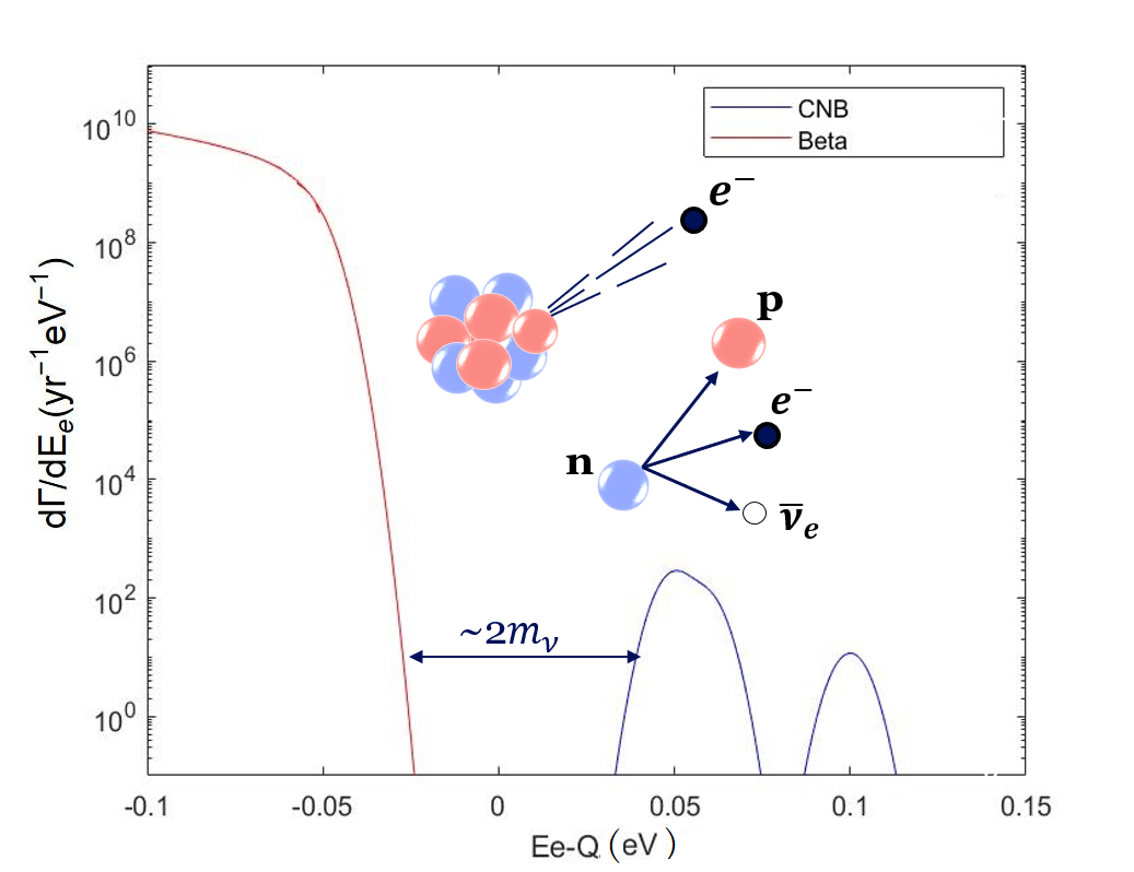
Figure 1: Beta decay spectrum and the sketch of the beta decay process. The blue curve depicts the C$\nu$B spectrum, and the red curve represents the beta decay spectrum, and they are separated by an energy gap, which has an order of magnitude twice the neutrino mass ($2m_{\nu}$). The annotation of the horizontal axis is the kinetic energy of the emitted electron measured from the endpoint of the beta decay spectrum, and the annotation of the vertical axis is the events observed at a certain energy per yer. The area behind each cure represents the events per year, and the area behind the C$\nu$B curve is only 4.

II Formulation of the problem

In this section, we formulate the mathematical model of beta-emission on graphene. This section is structured as follows, firstly, we give the physical description of the problem; then we list our main assumptions; then, we explain the approximation scheme used for the calculation of the observed emission line.

We consider a beta-emitter atom attached to a graphene sheet either by the Van der Waals force or through the formation of a chemical bond. After capturing an incoming neutrino, the beta-emitter converts into a daughter isotope, releasing a fast outgoing electron as depicted in Fig(2). The sudden emergence of a positively charged daughter isotope ion next to the graphene sheet triggers local rearrangement the material’s electronic structure, in the exact same manner as a core hole in an X-ray emission experiment does. In the latter case, such a rearrangement is known to result in the X-ray edge singularity in the emission spectrum, which is seen as broadening of the emission line into an asymmetric shape having a power-law singularity at the emission edge. A similar phenomenon will occur in the $\beta$-spectrum of a radioactive atom on graphene.

One remark is in order here. Due to the work function difference, an atom attached to graphene would typically donate or accept a number of electrons. This effect is characterised by the atom’s equilibrium charge state, that is the atomic number less the average total number of electrons occupying its atomic shells in equilibrium. For an mother isotope $\prescript{A}{Z}{X}$ in the charge state $Q$ the dominant decay channel will be into a daughter isotope $\prescript{A}{Z+1}{X}$ in the charge state $Q+1,$

$$\nu_{e}+\prescript{A}{Z}{X}^{Q}\to\ \prescript{A}{Z+1}{X}^{Q+1}+e^{-}.$$ (3)

Depending on the chemistry of the graphene-atom interaction $\prescript{A}{Z+1}{X}^{Q+1}$ may or may not be an equilibrium charge state. If this state is not equilibrium, it will decay into an equilibrium charge state after some time $\tau.$ By virtue of Heisenberg’s principle, this will introduce an additional $\hbar/\tau$ uncertainty into the energy conservation law for the products of the decay and consequently into the energy of the beta-electron. As will be discussed later in this work, in order for the neutrino capture peak to be observable, the life time of $\prescript{A}{Z+1}{X}^{Q+1}$ has to be quite long, for example it would have to to be longer than $10^{-2}\,\rm s$ for the ${}^{3}\rm He^{+}$ ion formed after the decay of neutral Tritium. Such long lifetimes require that either the atom be well insulated from graphene, for example by a thin layer of a wide gap insulator, or $\prescript{A}{Z+1}{X}^{Q+1}$ is an equilibrium charge state. The discussion of strategies for making $\prescript{A}{Z+1}{X}^{Q+1}$ a long-lived state is outside the scope of the present work and it will be addressed elsewhere. It is worth noting that in a situation where the charge state of the daughter $\prescript{A}{Z+1}{X}^{Q+1}$ is metastable there always exists a direct matrix element for the process in which the daughter atom is created in the stable state $\prescript{A}{Z+1}{X}^{Q^{\prime}}$ and the charge balance is taken care of by creation of elementary excitations in graphene. Due to insufficient kinematic constraints, such a few body process does not result in a sharp neutrino absorption peak. Rather, it forms a broad feature at the tail of the Lorentzian distribution of the absorption resonance defined by the metastable state.

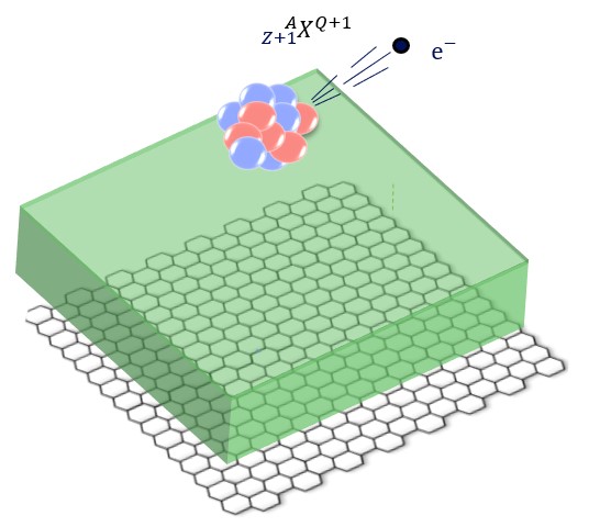
Figure 2: Sketch of the beta emitter and graphene sheet. $\prescript{A}{Z+1}{X}^{Q+1}$ is the production of the beta decay process, and it introduces a sudden localized perturbation in the electron system of graphene. This sudden localized perturbation causes an X-ray edge, which changes the beta decay spectrum. The thin green layer is a spacer inserted between the beta emitter and the graphene sheet to isolate the daughter isotope $\prescript{A}{Z+1}{X}^{Q+1}$ from the graphene sheet. Thus it improves the lifetime of $\prescript{A}{Z+1}{X}^{Q+1}$.

We can now state the main assumptions about the system that will enable us to focus on the Fermi sea shakeup effect
(1) The recoil of the daughter ion from the beta decay will be neglected. This effect and its mitigation strategies have been addressed in recent literature [17, 27, 28, 18]. Although significant on the $10\,\rm meV$ scale, this effect is not directly related to the Fermi sea shakeup discussed here.
(2) We neglect the electron-electron scattering in the graphene sheet. We include the Coulomb interaction between electrons only in the form of the Random Phase Approximation (RPA) [29, 30] corrections to the dielectric response of graphene.
(3) We only focus on the processes which do not result in the excitation of internal degrees of freedom of the daughter ion. Only such processes are relevant to the neutrino capture experiment.
(4) We assume that the graphene sample spatially uniform. Where we analyse the effect of disorder, we assume that the disorder is spatially uniform.
(5) We neglect crystalline lattice effects arising from the the lateral position of the beta-decayer relative to the graphene sheet. This is because the X-ray edge singularity is an infrared phenomenon, arising from the long-range Coulomb interaction, which is insensitive to the exact position of the Coulomb centre inside the unit cell.
(6) We assume for simplicity that the initial charge state of the beta-decayer is neutral.
(7) We assume that the beta-decay of the nucleus produces a long-lived daughter ion. The quantitative meaning of long-lived will be elaborated later.
(8) We assume that the temperature of the system is less than the resolution of the detector, which is about 100K. We thus neglect thermal effects and consider our model at zero temperature.

Based on the above assumptions, we formulate the Hamiltonian

$$H=H_{0}+H_{w}+H_{D-G}$$ (4)

which comprises the kinetic part, weak interaction part and the coupling between the daughter ion and graphene. The kinetic part is trivial, and it is the total relativistic energy of free motion of all particles involved in the process

$$H_{0}=H_{\nu}+H_{D}+H_{M}+H_{e}+\sum_{s}\sum_{k}s\hbar v_{F}kC^{\dagger}_{ks}C_{k^{\prime}s}$$ (5)

Here $\nu$ stands for the neutrino, $e$ for the electron, $M$ and $D$ for the mother and the daughter isotopes respectively, $v_{F}$ is the Fermi velocity $C^{\dagger}_{ks}$ and $C_{ks}$ are the creation and annihilation operators for the electrons in the graphene respectively, and s is the band index of the graphene. The spin and valley indices have been absorbed into the band index.

The term

$$H_{w}=\int G_{F}\nu MD^{\dagger}e^{\dagger}d^{3}x,$$ (6)

is the effective Hamiltonian of the beta-decay process, where $\nu^{\dagger}$ is the creation operator for the neutrino, $D^{\dagger}$ is the creation operator for the daughter ion, and $M$ is the annihilation operator for the mother isotope atom, $e^{\dagger}$ is the creation operator for the outgoing electron, and $G_{F}$ is the effective beta decay interaction constant absorbing the details of ultrafast electroweak processes inside the nucleus [10, 31],
The final term in the Hamiltonian, $H_{D-G}$ describes the interaction between the electrons in graphene and the charged daughter ion, which suddenly emerges due to the beta-decay process. Since the the daughter ion is very heavy and therefore can be treated as a localised object , we can write its density operator as $D_{0}^{\dagger}D_{0}\delta(\mathbf{r})$, where the origin $\mathbf{r}=0$ coincides with the equilibrium position of the mother atom and $D_{0}^{\dagger}D_{0}$ is the daughter ion counting operator. Thus we write this interaction term as follows

$$H_{D-G}=-\int\rho(x)V(x)D^{\dagger}_{0}D_{0}d^{2}x.$$ (7)

where

$$V(x)=\frac{e^{2}}{4\pi\epsilon\epsilon_{0}\sqrt{d^{2}+x^{2}}}$$ (8)

is the Coulomb pontential of the ion in the graphene plane, and

$$\rho(x)=:\psi^{\dagger}(x)\psi(x):,$$ (9)

is the two-dimensional density of electrons in graphene. We have denoted the dielectric constant of the graphene as $\epsilon$ and the distance between the daughter ion and the graphene as $d$. The field operator of an electron in graphene $\psi(x)$ admits for the standard plane wave decomposition

$$\psi(x)=\sum_{k,s}C_{ks}\psi_{ks}e^{-i\vec{k}\vec{x}}$$ (10)

where $\psi_{ks}$ is the spinor of the dirac electrons in the graphene,

$$\psi_{ks}=\frac{1}{\sqrt{2}}\begin{pmatrix}e^{-i\theta_{k}}\\ s\end{pmatrix}$$ (11)

with $\theta_{k}=\arctan(k_{y}/k_{x})$.

In the standard vein of beta decay theory, the transition probability is given by Fermi’s golden rule

$$W=\frac{2\pi}{\hbar}\sum_{f}\biggl{|}\left<0\right|_{t}\left<0\right|_{\nu}\left<k\right|_{e}\left<1\right|_{h}\left<\lambda\right|\int G_{F}\nu dh^{\dagger}e^{\dagger}d^{3}x\\ \left|1\right>_{t}\left|1\right>_{\nu}\left|0\right>_{e}\left|0\right>_{h}\left|FS\right>\biggr{|}^{2}\delta(E_{f}-E_{i})$$ (12)

where $f$ refers to the final states of the process, and $\left|\lambda\right>$ is the final eignstate of the graphene Hamiltonian with the energy $E_{\lambda}$ and $\left|\rm FS\right>$ is the Fermi sea of the graphene electrons characterised by the ground state energy $E_{0}$. The total energy of final state in the process is $m_{e}c^{2}+\frac{\hbar^{2}k^{2}}{2m_{e}}+E_{\lambda}+m_{D}c^{2}$, and the energy of initial state is $m_{v}c^{2}+m_{M}c^{2}+E_{0}$. The final state is the tensor product of the neutrino state, the outgoing electron state, and the graphene electron state. We can sum over the normal beta decay part and graphene part independently. We use index $f^{\prime}$ to denote the final state of beta decay and use index $\lambda$ to denote the final state of electrons in graphene. Moreover, we can express the total transition probability as a convolution of the transition probability function of beta decay and graphene spectral density function. Hence, the expression of the total transition probability can be simplified to

$$W=\frac{2\pi}{\hbar}\int dE\sum_{f^{\prime}}\sum_{\lambda}|V_{if^{\prime}}|^{2}|\left<\lambda|FS\right>|^{2}\delta(E+E_{\lambda}-E_{0})\\ \times\delta(E_{k}-Q-E)\\ =(\Gamma*A)(E_{k}),\\$$ (13)

where $V_{if^{\prime}}$ is the weak interaction matrix element, $Q=m_{M}c^{2}+m_{v}c^{2}-m_{e}c^{2}-m_{D}c^{2}$ is the emission energy of beta decay, $E_{k}$ is the kinetic energy of the beta electron, $\Gamma(E)$ is the beta decay transition rate of a single atom in vacuum, and $A(E)$ is the electron spectral density function in graphene. Note, that the energy conservation law in Eq. (LABEL:fermi) neglects the kinetic energy of both the heavy particles and the neutrino. The latter is due to the fact that we are interested in the narrow vicinity of the endpoint of the beta decay spectrum, furthermore, the temperature of the cosmic neutrino background, $1.95\,\rm K$, is negligible compared to the neutrino’s mass. Therefore, eq. (LABEL:fermi) both applies for beta decay background and the cosmic neutrino absorption process. Following the convention, we can consider ${d\tilde{\Gamma}}/{dE_{k}}$ as observable beta decay rate at given electron kinetic energy corrected by the electron shakeup process

$$\frac{d\tilde{\Gamma}}{dE_{k}}={\color[rgb]{0,0,0}N}\frac{dW}{dE_{k}}={\color[rgb]{0,0,0}N}\left(\frac{d\Gamma}{dE_{k}}*A\right)(E_{k}),$$ (14)

where $N$ is the number of beta-decayers deposited on graphene. The discussion above also valid for the process of background neutron decay. We have found out that the smeared beta decay spectrum is nothing but the convolution between the spectral density function of graphene and the original beta decay spectrum. This result is vital to us since it tells us the influence of the X-ray edge in the PTOLEMY project. Later, we will show that the spectral density function does have an X-ray edge.

III Linked Cluster Expansion

In this section we assume that daughter ion is screened instantaneously. This assumption does not work well in graphene and we will revise it later, however at this stage we would like to keep our discussion as simple as possible focusing on the key physics of the problem. With the help of the RPA and neglecting time retardation, we obtain the effective static dielectric constant of graphene [33]

$$\epsilon=\frac{1+\kappa}{2}+\frac{2\pi e^{2}}{q}\frac{g_{s}g_{v}q}{16\hbar v_{F}}$$ (15)

where $\kappa$ is the external dielectric constant of the substrate, the degeneracy factor $g_{s}=2,g_{v}=2$, and $v_{F}\approx 10^{6}\ \mathrm{m/s}$. If the graphene is suspended in vacuum, then $\epsilon\approx 4.4$.

The spectral density function $A(E)$ is the central object of interest, so we will investigate its property further in this section. The expression for it is

$$\begin{split}A(E)&=\sum_{\lambda}\left|\left<\lambda|FS\right>\right|^{2}\delta(E+E_{\lambda}-E_{0})\\ &{\color[rgb]{0,0,0}=\frac{1}{2\pi\hbar}\sum_{\lambda}\int dt\left<FS\right|e^{-iH_{g}t}\left|\lambda\right>\left<\lambda|FS\right>e^{-i\left(E-E_{0}\right)t/\hbar}}\\ &=\frac{1}{2\pi\hbar}\int dt\left<FS|e^{-iH_{g}t/\hbar}|FS\right>e^{iE_{0}t/\hbar}e^{-iEt/\hbar},\end{split}$$ (16)

where $H_{g}$ is the Hamiltonian of the graphene after the beta decay. We can express it in momentum space [33, 34],

$$H_{g}=\sum_{s}\sum_{k}s\hbar v_{F}kC^{\dagger}_{ks}C_{k^{\prime}s}\\ -\frac{1}{L^{2}}\sum_{ss^{\prime}}\sum_{kk^{\prime}}V(k,k^{\prime})F_{ss^{\prime}}(k,k^{\prime})C^{\dagger}_{ks}C_{k^{\prime}s^{\prime}}$$ (17)

with

$$F_{ss^{\prime}}(k,k^{\prime})=\frac{1}{2}\left[ss^{\prime}+\exp(i\theta_{k}-i\theta_{k^{\prime}})\right]$$ (18)

and

$$V(k,k^{\prime})=\frac{2\pi e^{2}\exp\left(-|k^{\prime}-k|d\right)}{\epsilon|k-k^{\prime}|}$$ (19)

To calculate the spectral density function $A(E)$, we first focus on the density function, which is its Fourier transform

$$\rho(t)=\left<\mathrm{FS}\left|\mathrm{e}^{-iH_{g}t/\hbar}\right|\mathrm{FS}\right>\mathrm{e}^{iE_{0}t/\hbar}.$$ (20)

One can recognize $-i\Theta(t)\rho(t)$ as the core hole Green function in the conventional X-ray singularity problem [35, 22, 23, 36, 29]. Using linked cluster expansion method [29, 37, 38], we can express the density function $\rho(t)$ in another way.

$$\rho(t)=\exp\left[\sum_{l}F_{l}(t)\right]$$ (21)

where $F_{l}(t)$ is the l-th connected diagrams,

$$F_{l}(t)=\frac{(-i)^{l}}{l}\int_{0}^{t}dt_{1}\cdots\int_{0}^{t}dt_{l}\left<TV(t_{1})\cdots V(t_{l})\right>_{\mathrm{connected}}.$$ (22)

$V(t)$ is the interaction term in the Dirac picture. We note that $F_{1}(t)=-iE_{i}t$ where the constant $E_{i}$ is called the self energy. The self energy is responsible for the overall energy shift of the beta spectrum relative to the vacuum one. Assuming the interaction is weak, we can restrict ourselves to the second term [29].

$$F_{2}(t)=-\int_{0}^{\infty}\frac{du}{u^{2}}R_{e}(u)(1-\mathrm{e}^{-iut})$$ (23)

where

$$R_{e}(u)=\frac{1}{\pi L^{2}}\sum_{q}|V(q)|^{2}\Lambda(q,u)$$ (24)

and

$$\Lambda(q,u)=\mathrm{Im}P^{(1)}(q,u).$$ (25)

where $P^{(1)}(q,u)$ is the polarizability function. The epxression of the polarizability is given in many references [29, 39], so we just quote the result

$$P^{(1)}(q,u)=\frac{-ig^{\prime}}{L^{2}}\int_{-\infty}^{\infty}\frac{dE}{2\pi}\sum_{p,s,s^{\prime}}|F_{ss^{\prime}}(p,p+q)|^{2}\\ \times G_{ss}(p,E)G_{s^{\prime}s^{\prime}}(p+q,E+u),$$ (26)

where $G_{ss}(P,E)$ is the Green function for graphene, $g^{\prime}$ is the degeneracy, and it is $4$ for intrinsic graphene. The polarizabiltiy function of the intrinsic graphene was calculated in the references [40, 33, 41]. In particular, its imaginary part gives

$$\Lambda(q,u)=\frac{q^{2}}{4\sqrt{u^{2}-v_{F}^{2}q^{2}}}\Theta(u-v_{F}q).$$ (27)

To calculate $R_{e}(u)$, one needs to substitute eq. (27) into eq. (24). To simplify the calculation, we omit the exponential factor in the eq. (19), and the potential becomes

$$V(k,k^{\prime})=\frac{2\pi e^{2}}{\epsilon|k-k^{\prime}|}$$ (28)

Although this crude simplification is only valid near the edge of the spectral density function, it gives us a physics insight in the first step. Later, we will recover the effect of the distance d in the next section. Then we have

$$R_{e}(u)=gu,$$ (29)

where

$$g=\frac{e^{4}}{2\epsilon^{2}v_{F}^{2}}$$ (30)

Using the effective dielectric constant we get in the previous step, we can find $g\approx 0.125$. Substituting it into the expression of $F_{2}$, thus one can get

$$\begin{split}F_{2}(t)&=-g\int_{0}^{\xi_{0}}\frac{(1-e^{-iut})du}{u}\\ &\approx-g\int_{1/it}^{\xi_{0}}\frac{du}{u}\approx-g\ln(1+it\xi_{0})\end{split}$$ (31)

Note that due to the logarithmic divergence of the integral we had to use an arbitrary ultraviolet cutoff $\xi_{0}$ to complete the calculation. This cutoff parameter is important for the estimate of the visibility of the $\mathrm{C}\nu\mathrm{B}$ peak, therefore it cannot be chosen arbitrarily. The physical meaning and the value of $\xi_{0}$ will be clarified later.

The expression (31) is valid only for large enough $t$, that is $\xi_{0}t>>1$. The expression for the density function is obtained from eq. (31),

$$\rho(t)=\exp(-iE_{i}t-g\ln(1+it\xi_{0})),$$ (32)

where the self energy term $E_{i}$ can be absorbed into the exponent $E$ in the Fourier transformation in the later steps. It has no effect on shape of the spectral density function, but shift it by $E_{i}$.

IV Spectral density function

In this section, we give an explicit formula of the spectral density function of graphene. Furthermore, we investigate the influence of the height from the daughter ion above the graphene sheet, as well as the influence of disorder and the dynamical screening on the spectral density function.

The Fourier transform of eq. (32) gives the spectral density function of graphene at the given energy, and it is exactly the gamma distribution function.

$$\begin{split}A(\Omega)&=\int_{-\infty}^{\infty}\frac{dt}{2\pi}e^{-iEt}\rho(t)\\ &=\Theta(-\Omega)\frac{\exp(\Omega)}{\xi_{0}\Gamma(g)(-\Omega)^{(1-g)}}\end{split}$$ (33)

with

$$\Omega=(E+E_{i})/\xi_{0}$$ (34)

The spectral density function obeys the gamma distribution, and the result coincides with that for a metal with a local constant interaction [29, 37, 38]. The gamma distribution function has two parameters: one is the shape parameter, which is the coupling constant in our problem, and another one is the scale parameter, which has so far remained an arbitrary cutoff parameter. The coupling constant determines how sharp the peak is near the edge, and the cutoff energy determines how many events are lost in the long tail of the spectral density function. Fig. 3 represents the spectral density function. As we can see in Fig. 3, the function sharply diverges when $\Omega$ goes to zero. In other words, the differential emission rate is the largest when no electron excitations are created in graphene at the end of the process.

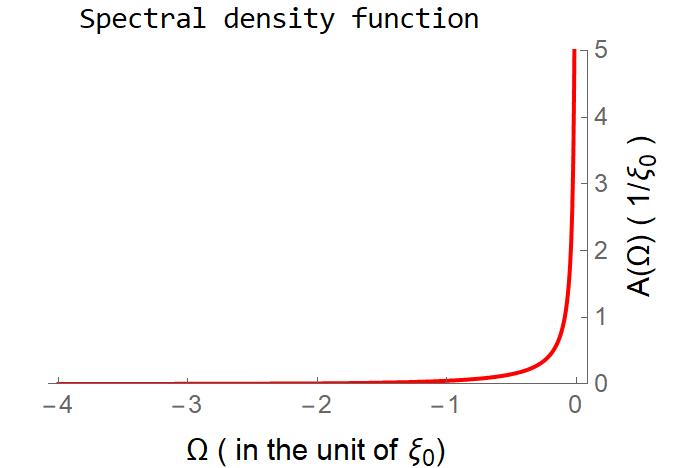
Figure 3: The spectral density function of graphene at a given energy. $A(\Omega)$ describes the possibility of graphene absorbing the outgoing electron’s energy. The energy is measured in the unit of cut-off energy $\xi_{0}$.

IV.1 Influence of the Height

In the previous discussion, we have calculated the spectral density function and obtained its shape parameter $g.$ However, the cutoff energy remains unknown. Typically, one would expects the cutoff energy to be associated with the electron bandwidth or the Fermi energy. In this section we find that the cutoff energy is dictated by the height of daughter ion above the graphene sheet. Indeed, for any given $d$ the expression of $R_{e}(u)$ is

$$\begin{split}R_{e}(u)=e^{4}\int_{0}^{u/v_{F}}\frac{qe^{-2qd}dq}{2\epsilon^{2}\sqrt{u^{2}-v_{F}^{2}q^{2}}}\\ =gu+\frac{\pi gu}{2}\left[L_{1}\left(\frac{2du}{v_{F}}\right)-I_{1}\left(\frac{2du}{v_{F}}\right)\right]\end{split}$$ (35)

where $L_{1}\left(\frac{2du}{v_{F}}\right)$ and $I_{1}\left(\frac{2du}{v_{F}}\right)$ are modified Struve function and modified Bessel function, respectively.
This equation may look slightly intimidating however its intuitive meaning is simple. The X-ray edge singularity is an infrared phenomenon, so only long distance interaction is significant for it. Thus we can eliminate the short-distance structure of the Coulomb interaction. If $q<<1/(2d)$, the Yukawa type potential in eq. (35) recovers to the normal Coulomb potential, thus giving a natural cutoff energy $\xi=\hbar v_{F}/2d$. From asymptotic analysis (details are in A1), we find that the spectral density function was the same form as in Eq. (33) albeit with a cutoff energy $\xi^{\prime}$,

$$\xi^{\prime}=\frac{\xi_{0}}{1+2d\xi_{0}/v_{F}}.$$ (36)

$\xi_{0}$ is a microscopic parameter on the order of the bandwidth energy. Assuming that $\xi_{0}\gg v_{F}/d$, one finds

$$\xi=\lim_{\xi_{0}\to\infty}\xi^{\prime}=\frac{\hbar v_{F}}{2d}$$ (37)

The expression (37) should replace $\xi_{0}$ as the scale factor in the line shape equation Eq. (33). One can see that the scale factor depends on the height $d,$ so one could potentially manipulate the line shape by adjusting the height of the ion.

IV.2 Influence of disorder

Until now, we have only considered intrinsic graphene, uncontaminated and ungated. However, a finite density of beta emitters in graphene inevitably introduces disorder, which changes the mean free path and the density-density response function of electrons. Intuitively, one should expect that if the time scale associated with the inverse energy resolution of the beta detector is greater than the mean free time in graphene, i.e., $\tau_{\mathrm{res}}\gg\tau$, then one needs to take into consideration the effect of electron diffusion on the polarizability function and thus the coupling constant.

We consider eq. (16), in the presence of many random impurities, focusing on the impurity-average effect. The impurity-average polarizability function $P_{\mathrm{imp}}(q,\omega)$ is [30, 42, 39]

$$P_{\mathrm{imp}}(q,\omega)=\frac{P^{(1)}(q,\omega+\frac{i}{\tau})}{1+(1-i\omega\tau)^{-1}\left[\frac{P^{(1)}(q,\omega+\frac{i}{\tau})}{P^{(1)}(q,0)}-1\right]}$$ (38)

where $\tau$ is the momentum relaxation time of a quasiparticle. The required energy resolution of the detector is $\omega_{\mathrm{res}}$ is about 10 meV, therefore the resolution time $\tau_{\rm res}$ is $\sim 10^{-13}\ s$. If $\tau>\tau_{\rm res}$, then one can neglect the effect of impurities, and the polarizability function recovers to the Lindhard function [30]. Otherwise, one needs to consider both diffusive and ballistic regimes.

To get some insight into the degree of coverage at which it is necessary to take the impurity scattering into consideration, we give an elementary estimate based on the mean free time calculated within the midgap model which is known to work reasonably well for hydrogen and other atoms with covalent on-site bonding on graphene [43, 44, 45]. In this model, mobility electrons in graphene see a carbon site with attached hydrogen as a vacancy. The potential is profiled as

$$U(r)=\begin{cases}\infty,&\mbox{if }0<r\leq R^{\prime}\\ U_{0},&\mbox{if }R^{\prime}<r\leq R\\ 0,&\mbox{if }r>R,\end{cases}$$ (39)

where $R^{\prime}$ is the the radius of a hydrogen atom, and $R$ is the radius of a carbon atom. The mean free time is defined from the following expression

$$\frac{\hbar}{\tau_{k}}=\frac{8n_{i}}{\pi\rho(E_{k})}\sin^{2}\delta(k),$$ (40)

where $\delta(k)$ is the phase shift of electrons with momentum k, and $\rho(E_{k})$ is the density of state, with the explicit form

$$\rho(E_{k})=\frac{2E_{k}}{\pi\hbar^{2}v_{F}^{2}}.$$ (41)

Using the method in the paper [44], we can obtain the phase shift at $k\approx 0$,

$$\delta(k)=-\frac{\pi}{2}\frac{1}{\ln(2kR^{\prime})}.$$ (42)

We expand the sine function in eq. (40) for $kR^{\prime}\ll 1$. Thus it gives the mean free time

$$\begin{split}\tau_{k}&=\frac{\hbar\rho(E_{k})}{2\pi n_{i}}(\ln kR^{\prime})^{2}\\ &=\frac{k}{\pi^{2}v_{F}n_{i}}(\ln kR^{\prime})^{2},\end{split}$$ (43)

where $n_{i}$ is the impurity concentration. The mean free path has a minimal value at $kR^{\prime}=\mathrm{e^{-2}}$, and its minimum value is

$$\tau_{min}=\frac{4\mathrm{e^{-2}}}{\pi^{2}v_{F}n_{i}R^{\prime}}$$ (44)

If $\tau_{min}$ is much greater than the resolution time, we can neglect the impurity effect. It means that

$$\frac{4\mathrm{e^{-2}}}{\pi^{2}v_{F}n_{i}R^{\prime}}\gg 1/\omega\sim 10^{-13}\ s$$ (45)

$R^{\prime}$ is about 1 $\mathrm{\SIUnitSymbolAngstrom}$, so we find the condition for a maximum impurity concentration.

$$n_{i}\ll\frac{4\mathrm{e^{-2}}\omega}{\pi^{2}v_{F}R^{\prime}}=5\times 10^{11}/\mathrm{cm^{2}}$$ (46)

To conclude, for atoms in the onsite boding configuration the effect of disorder is negligible for surface coverage of less than $5\times 10^{11}/\mathrm{cm^{2}}.$ For atoms in other configurations the critical concentration could be different, even though we do not expect the difference to be dramatic. If impurity atoms are separated from graphene by an thin layer of insulator the critical coverage may be significantly greater.

Apart from impurities, phonons can also influences the mean free time of graphene. However, one can keep the system in a very low temperature to reduce the phonon scattering. For intrinsic graphene under liquid nitrogen temperature, the momentum relaxation time is about one ps [46, 47], which is one order of magnitude greater than the resolution time. Therefore, we can treat electrons of the graphene ballistically within the resolution time.

IV.3 Influence of Dynamic Screening

The instantaneous screening assumption is not valid in the tail of the spectral function of graphene. While, if the weight of the tail is too high, it will cause the beta decay spectrum to broaden widely, and it may take many years to observe a single event. To get a more rigorous result, we need to consider the dynamic screening effect. The dynamic screening potential is [29]

$$V(q,\omega)=\frac{V_{i}(q,\omega)}{\epsilon(q,\omega)}$$ (47)

For a sudden external potential [48],

$$V_{i}(q,\omega)=\frac{V(q)i}{\omega+i\delta}.$$ (48)

$\delta$ is an infinitesimal quantity, and $V(q)={2\pi e^{2}}/{(\kappa q)}$ is the bare Coulomb potential with $\kappa$ the external dielectric constant of the substrate. We notice that $\epsilon^{-1}(q,\omega)-1$ is the susceptibility function so we can use the Kramers-Kronig relations.

$$\frac{1}{\epsilon(q,\omega)}-1=-\frac{1}{\pi}\int_{-\infty}^{\infty}d\omega^{\prime}\mathrm{Im}\left(\frac{1}{\epsilon(q,\omega^{\prime})}-1\right)\frac{1}{\omega-\omega^{\prime}+i\delta}$$ (49)

Substituting it into the expression of dynamic screening potential and performing the Fourier transform, one can find the time-dependent screening potential.

$$\begin{split}V(q,t)&=\int_{-\infty}^{\infty}V(q,\omega)\mathrm{e}^{-i\omega t}d\omega\\ &=\frac{V(q)\theta(t)}{\pi}\int_{-\infty}^{\infty}\frac{1-\mathrm{e^{-i\omega^{\prime}t}}}{\omega^{\prime}}\mathrm{Im}\left(\frac{1}{\epsilon(q,\omega^{\prime})}-1\right)d\omega^{\prime}\\ &\quad\quad\quad\quad\quad\quad+V(q)\theta(t)\\ \end{split}$$ (50)

In the large time limit, the oscillating term disappears, so the potential becomes

$$V(q,\infty)=\frac{V(q)}{\epsilon(q,0)}$$ (51)

For graphene, $\epsilon(q,0)$ does not depend on q, so that we can denote $\epsilon(q,0)$ as $\epsilon$. The first term in the last line vanishes in the short time limit, so the potential turns into the bare potential.

$$V(q,0)=V(q)$$ (52)

For an arbitrary time, we can express $V(q,t)$ as

$$V(q,t)=\frac{V(q)\theta(t)}{\epsilon(q,0)}-\frac{V(q)\theta(t)}{\pi}\int_{-\infty}^{\infty}d\omega^{\prime}\frac{\mathrm{e^{-i\omega^{\prime}t}}}{\omega^{\prime}}\\ \times\mathrm{Im}\left(\frac{1}{\epsilon(q,\omega^{\prime})}-1\right)$$ (53)

From detailed analysis (see A2), we found out that the spectral density function is the same as the previous result in eq. (33), but with a different coupling constant

$$g_{1}=g+\int_{1}^{\infty}\frac{2g\epsilon}{\pi}\frac{a\log(\omega+\sqrt{\omega^{2}-1})}{\omega^{2}\left(\omega^{2}-1+a^{2}\right)}d\omega,$$ (54)

where $a=(\epsilon-1)={\pi e^{2}}/{2\hbar\kappa v_{F}}$, and this result is quoted from the A2 eq. (78 ). It is similar in meaning to the fine structure constant in QED.

If graphene is suspended in vacuum, then $g=0.125$, and $g_{1}\approx 0.200$. For graphene on ${\rm SiO}_{2}$, the coupling constant g is about 0.065, and $g_{1}\approx$ 0.090 . As one can see in Fig. 4, the dynamic screening effects of intrinsic graphene significantly change the coupling constant at a small dielectric constant, and this can be understood intuitively. For intrinsic graphene, the Fermi energy is zero, therefore there is no intrinsic time scale. For long wave-length scattering, the screening time is about $1/(v_{F}q)$, which is also the time scale for the Fermi sea shakeup effect at the energy scale $v_{F}q$, so we cannot separate the screening of the Coulomb potential from the formation of the X-ray edge singularity. Hence, the dynamical screening effects have a considerable influence on the coupling constant. In contrast, the Fermi energy is non-zero for normal metals and gated or doped graphene, so the static screening is a good approximation near the edge in those cases. In the large dielectric constant limit, one can see from Fig. 4(b), the ratio of the dynamic coupling constant and static coupling constant approaches 1. It can be understood from eq. (15) and eq. (54), when the external dielectric constant is big enough, it makes the dominant contribution to the total dielectric constant.

To summarize, the dynamical screening effect has a considerable influence on the coupling constant in intrinsic graphene, but it can be suppressed by applying an external gate voltage or increasing the dielectric constant of the substrate.

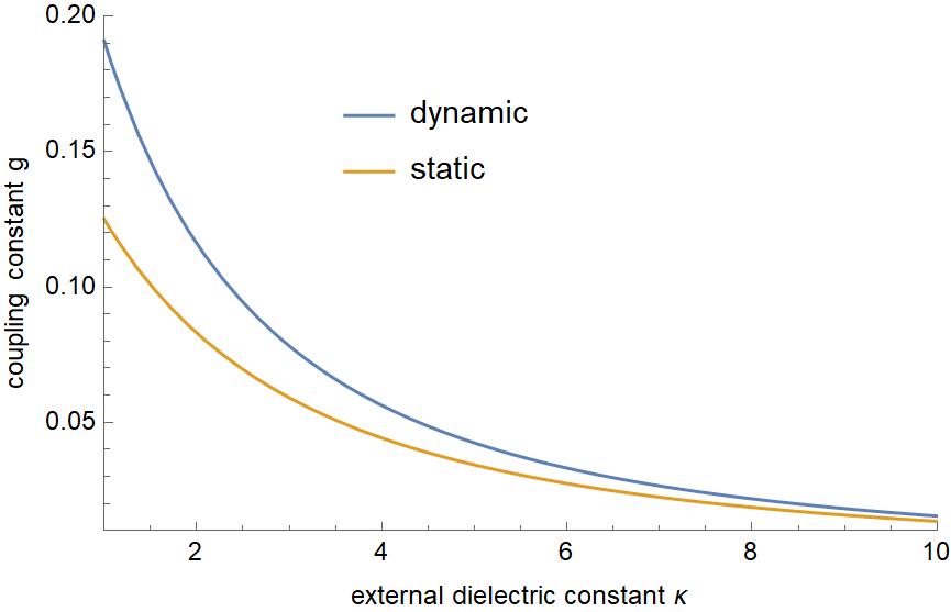
(a)

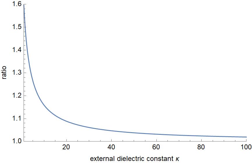
(b)

Figure 4: Fig. 4(a) depicts the coupling constant with different external dielectric constants. $\kappa$ describes the dielectric constant of the substrate, and g is the graphene’s coupling constant. The blue curve represents the coupling constant considering the dynamic screening effect, and the orange curve representing the coupling constant in the static screening approximation. Fig. 4(b) describes the ratio of the dynamic coupling constant and the static coupling constant. In the large dielectric constant limit, the ratio approaches 1.

IV.4 Constraints on the Daughter Ion’s Lifetime

In the previous discussion, we assumed that the lifetime of the daughter ion is infinite, however in reality this may not be true. The daughter ion could be chemically unstable and have propensity to, for example, capture an electron from its chemical environment. By virtue of Heisenberg’s principle shorter life times would introduce greater uncertainty into the measured energy of the beta electron. In the conventional X-ray edge singularity context the life time of an ion is limited by the process of recombination of a conductance electron with the core hole. Such a process requires accommodation of a large amount of energy which is usually achieved through the Auger effect. In the case of an ion which is formed through beta decay, the electron deficit occurs in the chemically active outer shell therefore capture of an electron may be possible through a direct tunneling process. The efficiency of such a process will vary depending on the way an atom is deposited on the surface. Insertion of a dielectric spacer between the atom and a graphene layer, or deposition of atoms in the form of self-assembled metal-organic complexes [50] could be possible ways to make the life time of the daughter ion longer. Ideally, one should aim to tune the chemical environment so as to make the daughter ion chemically stable. Somehow or other, the life time of an ion formed after the beta decay process is determined by a range of environmental mechanisms and is a matter for the experiment to measure and manipulate. Here, we do not attempt to estimate it. Rather we investigate how the finite life time of the daughter ion influences the visibility of the $\mathrm{C}\nu{\mathrm{B}}$ signal.

Semi-empirically, one absorbs the effects of a finite life time into the Lorentzian broadening of the delta function representing the energy conservation law. For the spectral density function that amounts to an extra convolution [29].

$$A(E)\mapsto\int_{-\infty}^{\infty}A(\mathcal{E})L(E-\mathcal{E})d\mathcal{E}$$ (55)

where $L(E)$ is the Lorentzian distribution function,

$$L(E)=\frac{\gamma/2}{\pi[E^{2}+(\gamma/2)^{2}]}.$$ (56)

$\tau=\hbar/\gamma$ is the lifetime of the daughter ion. The thus deformed spectral function should then be used in Eq. (14) to describe the observable beta spectrum. In particular, inserting eq. (56) into eq. (55), one obtains the shape of the spectral density function

$$A(E)=\operatorname{Im}\left[\frac{\mathrm{e}^{\tilde{\Omega}}\Gamma(1-g,\tilde{\Omega})}{\pi\xi_{0}\tilde{\Omega}^{1-g}}\right],$$ (57)

where $\Gamma(x,y)$ is the incomplete gamma function and

$$\tilde{\Omega}=\frac{E-i\gamma/2}{\xi_{0}}=\Omega-\frac{i\gamma}{2\xi_{0}}.$$ (58)

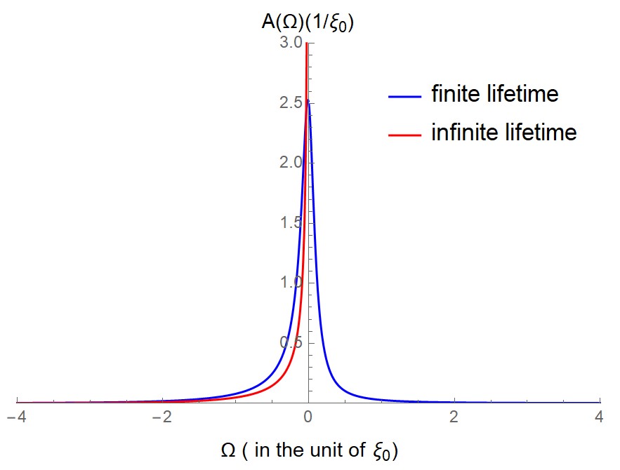
Figure 5: The spectral density function taking into account the influence of the finite lifetime of the daughter ion (blue curve) is compared with the spectral density function at infinite life time (red curve). As one can see, at finite life time the the sharp Gamma distribution is broadened into a smooth asymmetric peak. In this plot we take $g=0.125,$ $\xi_{0}=1\,\rm eV$ and $\gamma=0.2\,\rm eV.$

To illustrate such a shape, we plotted $A$ as a function of the dimensionless eneregy $\Omega$ for $g=0.125$, $\xi_{0}=1\ \rm eV$, and $\gamma=0.2\ \rm eV$ in Fig. 5. As one can see, at finite $\gamma$ the X-ray edge power law singularity gets deformed into an asymmetric bell-shaped distribution. The longer the life time, the closer the absorption peak is to the Gamma distribution (33).

While it is tempting to conclude that the main manifestation of a finite life time of the daughter ion is just some degree of broadening the neutrino absorption peak, which can be neglected for $\gamma\ll m_{\nu},$ on closer inspection the effect turns out to be a lot more detrimental and the conditions on $\gamma$ a lot more stringent. Moreover, the semi-empirical one-parameter model encapsulated in equation (56) turns out to be unsuitable for the quantitative analysis of the visibility of the $\rm C\nu\rm B$ peak. Indeed, unlike the pure X-ray edge singularity (33), the semi-phenomenological distribution (57) has a long power-law tail on the right-hand side of the peak

$$A(E)\sim\frac{\gamma}{E^{2}},\qquad E\gg\gamma$$ (59)

At the same time, the beta-decay background near the emission edge $E_{0}\approx Q$ has the parabolic shape

$$\frac{d\Gamma(E)}{dE_{k}}=\alpha\frac{N}{Q^{3}T}(E_{0}-E)^{2},\qquad E<E_{0}.$$ (60)

which remains a good approximation up to $E_{0}-E$ on the order of $Q.$ In this expression $\alpha$ is a nucleus-specific numerical constant on the order of 1 and $T$ is the half-life time. Due to the rapid increase of the background intensity away from the termination point $E_{0}$, the convolution (14) at energies slightly above the edge of the spectrum is completely dominated by the bulk of the beta spectrum and to a good accuracy can be expressed as

$$\frac{d\tilde{\Gamma}_{\rm BG}}{dE_{k}}=C+o(E-E_{0})$$ (61)

where

$$C=\frac{\gamma}{2\pi}\int_{0}^{Q}\frac{1}{(Q-\mathcal{E})^{2}}\frac{d\Gamma}{dE_{k}}(\mathcal{E})d\mathcal{E}\sim\frac{\gamma N}{Q^{2}}$$ (62)

In other words, the number of beta decay events as a function of the energy distance from the emission threshold increases so rapidly that it overwhelms the slow $1/E^{2}$ decay of the Lorentzian and thus creates a massive background in the region of the $\rm C\nu B$ peak. In reality, the fact that the main contribution to noise comes from the tail of the Lorentzian distribution invalidates the model (56) and the resulting estimate (62). To obtain the accurate result one would have to replace $L(E)$ with the exact ion’s spectral function. Although such a spectral function is impossible to calculate in practice, one can still make an order of magnitude estimate of the background intensity in the $\rm C\nu B$ peak region basing on the observation that the tail on the right-hand side of the resonant peak terminates at energies on the order of the ionisation energy of the recombined atom. More precisely, the termination point of the support of the ion’s spectral function is defined by the process of direct transition of the beta-decayer into the neutral daughter atom and a positively charged quasihole on graphene’s Fermi surface, which is the lowest energy out-state of the combined graphene - daughter atom system. In order to incorporate this physics into the semi-phenomenological model we introduce a truncated Lorentzian model in which $L(E)$ is given by Eq. (56) up to the first ionization energy $E_{I}$ of the daughter atom attached to graphene and vanishes for $E>E_{I}.$ Using such a truncation, the background will be approximately given by

$$\frac{d\tilde{\Gamma}_{\rm BG}(E)}{dE_{k}}\sim\frac{\gamma}{2\pi}\int_{E-E_{I}}^{E_{0}}\frac{1}{(E-\mathcal{E})^{2}}\frac{d\Gamma(\mathcal{E})}{dE_{k}}d\mathcal{E}.$$ (63)

Such a function describes of an $E_{I}$-wide tail of background events above the edge $E_{0}$ containing total events per unit time

$$\frac{dN_{\rm BG}}{dt}\sim\frac{E_{I}^{2}\gamma N}{TQ^{3}}.$$ (64)

To get some feel for the magnitude of this effect, we apply the estimate (64) to beta decay of Tritium neglecting for illustrative purposes the problems arising from recoil. A 100 g sample of Tritium contains $N=2\times 10^{25}$ atoms, and it is predicted to experience only 4 neutrino capture events per year. We take $E_{I}\sim 10\,\rm eV$ and $Q\sim 10\,\rm keV$ and $T\sim 10$ years and demand that $dN_{\rm BG}/dt$ be less than 1 event per year, which would roughly correspond to a $3\sigma$ detection confidence if 5 events are observed during the 1 year period. This results in the requirement $\gamma<10^{-14}\,\rm eV,$ that is a life time on the order of a few hundred milliseconds or longer. The condition on the relaxation time can in principle be relaxed if the energy window $(E_{0},E_{0}+\Delta E)$ containing the neutrino capture peak is known a priori. In that case, the number of background events inside that window is estimated as the right hand side of (64) times $\Delta E/E_{I}.$ For $\Delta E$ on the order of $100\,\rm meV$ that gives the lower bound on the ion’s life time of about $10\,\rm ms.$ This estimate is further elaborated in our numerical calculation, illustrated in Fig: 8, of the effective amount of the radioactive material required in order to achieve the p-value of $5\sigma$ in a $\rm C\nu B$ detection experiment using the energy bin of 100 $\rm meV$ above the spontaneous beta-emission threshold of Tritium.

V Discussion

In this section, we have investigated how the results of the previous sections translate into the visibility of the $\mathrm{C}\nu{\mathrm{B}}$ signal in the PTOLEMY experiment. From Eq. (14), we know that we can get the correct beta decay spectrum by performing a convolution between the spectral density function and the beta decay spectrum in vacuum. Using Mathematica, we plotted the beta decay spectrum with, $m_{\mathrm{lightest}}=50\,\rm meV$. As can be seen from comparison of Fig. 6(a) and Fig. 6(b), the shakeup of the electron system results in each cosmic neutrino background peak getting deformed into a strongly asymmetric shape peaking near the actual neutrino mass and having a long power-law tail stretching into the beta decay background. Note that the distortion of the beta-decay background is not as conspicuous as in the case of the C$\nu$B peak. The reason for that is that the distortion is a result of each individual beta-electron losing some part of its energy in order to create a collective excitation of electrons in graphene. That is why the distortion of the C$\nu$B peak results in signal appearing at lower energies in the gap between the C$\nu$B signal and the beta-decay background. At the same time the distortion of the beta-decay background just leads to a certain amount of re-distribution of electrons within the beta-decay continuum, without affecting the end point. The latter effect is difficult to see by the unaided eye, especially on the logarithmic scale. Using the calculated spectrum, we obtained the visibility, that is the number of events in the non-overlaping region in the spectrum. For the calculation of visibility we assume the amount of radioactive material equivalent to four capture events per year (about $100\,\rm g$ in the case of Tritium).

From our analysis it follows that the visibility depends on four parameters, the lightest neutrino mass, the coupling constant $g$, the distance from the daughter ion to the graphene sheet, and the lifetime of the daughter ion. We investigate the PTOLEMY project’s sensitivity to those parameters by making the plots of the visibility in different parameter planes.

In Fig. 7 we show the dependence of the visibility on the lightest mass of neutrino and the coupling constant $g$. As shown in Fig. 7, the smaller the coupling constant and the larger lightest mass of the neutrino, the better the visibility. This result can be explained by the fact that a smaller coupling constant leads to a sharper distribution, which causes the beta decay spectrum less broadening. The effect of the distance between the daughter ion and graphene is that it affects the cutoff energy and therefore influences the shape of the distorted beta-emission peak. Smaller cutoff energy means less weight in the long tail of the gamma distribution, therefore fewer losses and better visibility. Indeed, as one can see from Fig. 9, visibility increases with the helium ion’s height. Note that compared with the previous three parameters the influence of height on visibility is less pronounced, at least for a small enough coupling constant. This is explained by the fact that for small $g$ a lot of spectral weight is concentrated in the infrared region near the X-ray edge therefore the visibility is less sensitive to the ultraviolet cutoff.

Finally, a parameter that has a huge impact on the visibility of the $C\nu B$ signal is the lifetime of the daughter ion. In Fig. 8 we illustrate this point on the example of Tritium, even though this isotope suffers from problems arising from recoil. We see that in order to achieve the signal to noise ratio ensuring $5\sigma$ confidence of detection of the $C\nu B$ signal with a reasonable amount of the radioactive material the life time of the daughter ion needs to be greater than 100 $\mu s.$ Such a stringent requirement to the life time of the daughter ion poses a separate challenge to the experiment. Detailed proposals as to how this challenge could be addressed will be discussed elsewhere.

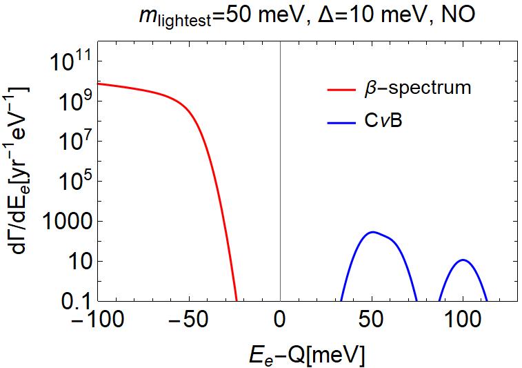
(a)

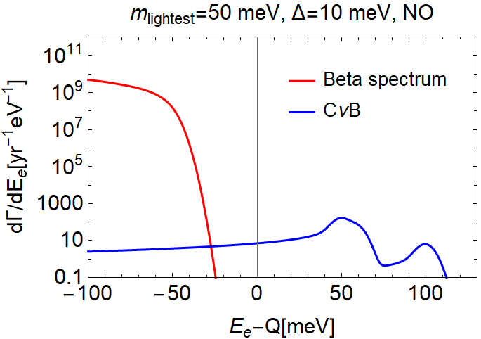
(b)

Figure 6: Panel 6(a) shows the theoretical beta decay spectrum of mono-atomic tritium in vacuum assuming the lightest neutrino mass of $50\,\rm meV$ The solid red curve represents the background beta decay. The solid blue curve represents the signal from the cosmic neutrino background. $d\Gamma/dE$ describes the possibility that the events happen at a given energy per year. The area under the curve represents the number of events per year. The area under the blue curve is only four, that is the calculation is done for the amount of Tritium that can capture at most four cosmic neutrinos per year. In the region where the beta decay background (red curve) overlaps with the $\mathrm{C}\nu\mathrm{B}$ (blue curve) one cannot distinguish the cosmic neutrino signal from noise. Panel 6(b) describes the beta decay spectrum adjusted for the Fermi sea shakeup effect. We choose the coupling constant $g=0.125$.

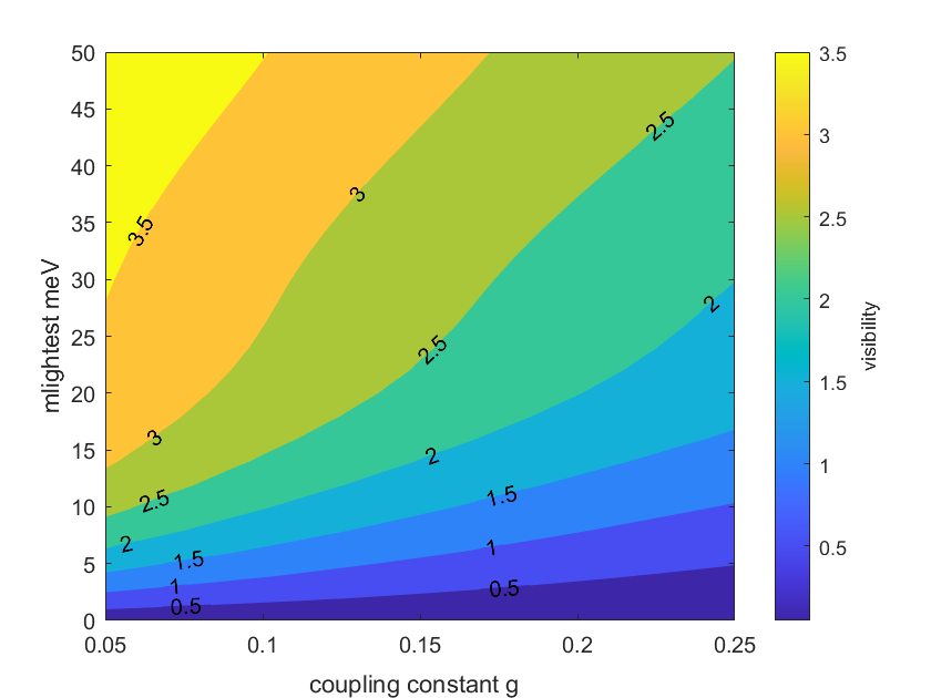
Figure 7: Contour plot of visibility as a function of the lightest mass of neutrino and the coupling constant. The cut-off energy is assumed to be $1\,\rm eV$. The maximum possible number of C$\nu$B events is 4.

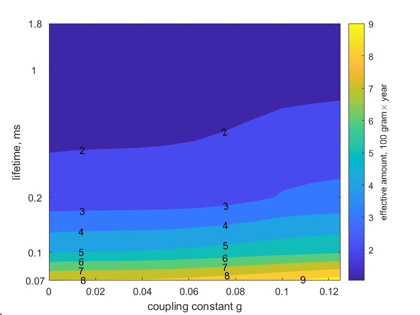
Figure 8: Contour plot of the effective amount of Tritium required in order to achieve the p value of 5$\sigma$ or better as a function of the coupling constant and the lifetime. The unit of the effective amount of tritium is $\rm 100\ gram\times year$, which means one can achieve the same necessary number of events by either increasing the amount of Tritium or increasing the duration of the experiment. The plot is calculated within the truncated Lorentzian model assuming the ionization energy $E_{I}=10\;\rm eV.$

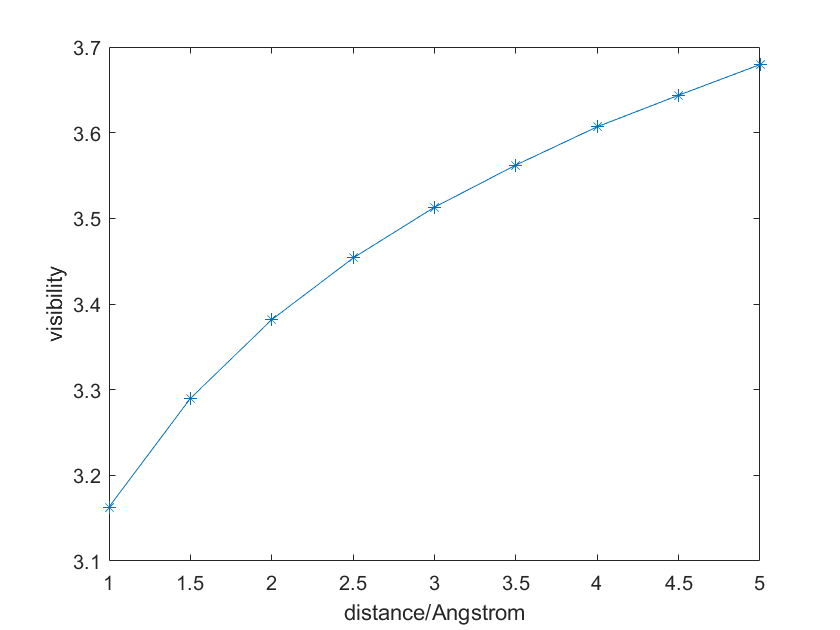
Figure 9: Visibility at different heights with coupling constant $g=0.1$, and $m_{\mathrm{lightest}}=50\ \mathrm{meV}$. The curves with different coupling constants and the neutrinos’ lightest mass share a similar feature.

VI Summary and outlook

In this work, we discussed how the shakeup of graphene’s Fermi sea may influence the visibility of the cosmic neutrino signal in the PTOLEMY project. In the first section, we used Fermi’s golden rule to find the beta decay spectrum adjusted for the Fermi sea shakup effect. We showed that it is the convolution between the spectral density function of a coulomb centre in graphene and the beta spectrum of the decaying isotope in vacuum. Furthermore, we applied the linked cluster expansion technique, to obtain the spectral density function, which is the Gamma distribution function and controlled by two parameters, the cutoff energy and the dimensionless coupling constant.

In the next section, we examined factors that influence the coupling constant and the cutoff energy, and we also considered the influence of the daughter ion’s lifetime on the spectral density function. We found that the distance between the ion and graphene dictates the natural distance-dependent energy cutoff scale. Also, the effects of disorder can be neglected if the mean free time of an electron in graphene exceeds the resolution time of the experiment, which is about $10^{-13}\,s.$ However, the dynamic screening effects of the intrinsic graphene significantly increase the coupling constant, which is detrimental to the visibility of the PTOLEMY project. Fortunately, if the external dielectric constant of the substrate is large enough, the dynamic screening effects can be suppressed. We further established that the lifetime of the daughter ion may have a hugely detrimental impact on the discernibility of $\rm C\nu B$ signal. To illustrate this point we show that for the decay of a reasonable amount of Tritium, the life time of the Helium ion would need to be at least $100\,\rm\mu s$ or longer.

Overall, we have three main conclusions.
(1) Our preliminary analysis indicates that despite large energy scales associated with the shakeup of the Fermi sea, the visibility can still be protected by the X ray edge singularity and screening effects. Even though we use the parameters of Tritium for numerical illustration, our results are universal and directly adaptable to any other atom.
(2) The visibility of the $\rm C\nu B$ signal can be improved in the following ways:
1) use a substrate with a high dielectric constant;
2) deposit the radioactive atoms in such a way as to maximize their distance from the graphene sheet, possibly with the help of a dielectric spacer
(3) Not all effects are included in our analysis, so experiments should be conducted to test the validity range of our theory. Also, the parameters such as the coupling constant $g$ and the lifetime of the daughter ion can only be reliably determined in an experiment.

We finally remark that although we have considered some important solid state effects that can affect the spectral density function, other effects require further study. Those include phonon emission, inhomogeneous broadening in a disordered sample, Coulomb interaction of the beta-electron with electrons in graphene and others. While such effects are not necessarily important in the traditional X-ray emission experiment, the extraordinary energy resolution required by the PTOLEMY experiment puts unusually stringent constraints on the admissible rate and magnitude of disruption due to various solid state processes. We hope that further research will improve our understanding of such effects and their mitigation.

VII Appendix

A1

The details of obtaining the natural cutoff energy are presented here.
Substituting eq. (35) into the eq. (23), one can find that

$$F_{2}^{\prime}(t)=-g\int_{0}^{\xi_{0}}\frac{(1-e^{-iut})du}{u}\\ -\frac{\pi g}{2}\int_{0}^{\xi_{0}}du\frac{(1-e^{-iut})}{u}\left[L_{1}(\frac{2du}{v_{F}})-I_{1}(\frac{2du}{v_{F}})\right]$$ (65)

The first integration is the original term, labeled as $F_{2}^{0}(t)$ and the second integration is the correction term, labeled as $F_{2}^{\prime}(t)$. Directly evaluating the correction term is difficult, but we can express it as a double integral.

$$F_{2}^{\prime}(t)=g\int_{0}^{2d\xi_{0}/v_{F}}\int_{0}^{1}e^{-zx}\sqrt{1-x^{2}}(1-e^{-izv_{F}t/2d})dxdz\\ =P(\xi_{0})+N(\xi_{0},t)$$ (66)

where

$$P(\xi_{0})=g\int_{0}^{1}dx\sqrt{1-x^{2}}\left(\frac{1-e^{-2dx\xi_{0}/v_{F}}}{x}\right),$$ (67)

and

$$N(\xi_{0},t)=g\int_{0}^{1}dx\sqrt{1-x^{2}}\left(\frac{-1+\exp(-it\xi_{0}-2dx\xi_{0}/v_{F})}{x+iv_{F}t/2d}\right)$$ (68)

with $z=2du/v_{F}$. From the calculation above, we can find that the correction term can be split into two terms. The first part is a constant independent of time t, and the second part is a time-dependent function. Hence, only the function $N(\xi_{0},t)$ is significant to our calculation. Obviously, if $t=0$, it cancels with the first term $P(\xi_{0})$. However, when t approaches infinity, the correction term $F_{2}^{\prime}(t)$ should equal to $P(\xi_{0})$. We need to make some approximations to evaluate the function $N(\xi_{0},t)$.
At a large time limit, roughly, we can use 1 to replace the ugly square root $\sqrt{1-x^{2}}$ since most contributions to the integration in $P(\xi_{0})$ and $N(\xi_{0},t)$ come from the vicinity of x=0. Then, we can write the correction term $F_{2}^{\prime}(t)$ in a simple way.

$$\begin{split}F_{2}^{\prime}(t)&=g\int_{0}^{1}\left(\frac{1-e^{-2dx\xi_{0}/v_{F}}}{x}\right)dx\\ &\quad+g\int_{0}^{1}dx\left(\frac{-1+\exp(-it\xi_{0}-2dx\xi_{0}/v_{F})}{x+iv_{F}t/2d}\right)\\ &=g\int_{0}^{1}\left(\frac{1-e^{-2dx\xi_{0}/v_{F}}}{x}\right)dx\\ &\quad-g\int_{iv_{F}t/2d}^{1+iv_{F}t/2d}\left(\frac{1-\exp(-2dy\xi_{0}/v_{F})}{y}\right)dy\\ &=g\int_{0}^{1}\left(\frac{1-e^{-2dx\xi_{0}/v_{F}}}{x}\right)dx\\ &\quad+g\int_{0}^{iv_{F}t/2d}\left(\frac{1-\exp(-2dy\xi_{0}/v_{F})}{y}\right)dy\\ &\quad-g\int_{0}^{1+iv_{F}t/2d}\left(\frac{1-\exp(-2dy\xi_{0}/v_{F})}{y}\right)dy\end{split}$$ (69)

The factor $1-\exp(-2dy\xi_{0}/v_{F})$ behaves as $2dy\xi_{0}/v_{F}$ in the limit $u\to 0$. We can use $\frac{v_{F}}{2d\xi_{0}}$ to replace the lower limit of the integration, since $\frac{v_{F}}{2d\xi_{0}}\ll 1$. At very large time t, we omit the factor $\exp(-2dy\xi_{0}/v_{F})$. Hence, the correction term $F_{2}^{\prime}(t)$ can be approximately expressed as a very neat form.

$$F_{2}^{\prime}(t)\approx g\int_{v_{F}/(2d\xi_{0})}^{1}\frac{dx}{x}+g\int_{v_{F}/(2d\xi_{0})}^{iv_{F}t/2d}\frac{dy}{y}\\ -g\int_{v_{F}/(2d\xi_{0})}^{1+iv_{F}t/2d}\frac{dy}{y}\\ \approx g\ln(1+\frac{2d\xi_{0}}{v_{F}})+g\ln(i\xi_{0}t+1)\\ -g\ln(i\xi_{0}t+\frac{2d\xi_{0}}{v_{F}}+1)$$ (70)

Substituting eq. (70) into equation (65), and using equation (21) and equation ((33)), one can obtain the expression of spectral density function of graphene.

$$\begin{split}A(\Omega^{\prime})&=\int_{-\infty}^{\infty}\frac{dt}{2\pi}e^{-iEt}\exp(F_{2}^{0}(t)+F_{2}^{\prime}(t)\\ &=\Theta(-\Omega^{\prime})\frac{\exp(\Omega^{\prime})}{\Gamma(g)\xi^{\prime}(-\Omega^{\prime})^{(1-g)}}\end{split}$$ (71)

where $\xi^{\prime}=\frac{\xi_{0}}{1+2d\xi_{0}/v_{F}}$, and $\Omega^{\prime}=(E+E_{i})/\xi^{\prime}$.
The cut-off energy $\xi_{0}$ is entirely arbitrary, but we can get a natural cut-off energy $\xi$ when we extend $\xi_{0}$ to infinity.

$$\xi=\lim_{\xi_{0}\to\infty}\frac{\xi_{0}}{1+2d\xi_{0}/v_{F}}=\frac{\hbar v_{F}}{2d}$$ (72)

We get nearly the same result as the previous one, eq. (33), only with different cutoff energy $\xi$.

A2

For intrinsic graphene, the time-dependent potential is

$$V(q,t)=\frac{V(q)\theta(t)}{\epsilon(q,0)}+V(q)\theta(t)T(v_{F}qt).\\$$ (73)

$T(v_{F}qt)$ is a one-variable fast-decay function that only depends $v_{F}qt$.

$$T(v_{F}qt)=-\frac{2}{\pi}\int_{1}^{\infty}\frac{a\cos(\omega v_{F}qt)\sqrt{\omega^{2}-1}}{\omega\left(\omega^{2}-1+a^{2}\right)}d\omega,$$ (74)

where $a=(\epsilon(q,0)-1)=\frac{\pi e^{2}}{2\hbar\kappa v_{F}}$. When $t<<1,T(v_{F}qt)\approx\frac{1}{\epsilon(q,0)}-1$, and when $t>>1,T(v_{F}qt)\approx 0$
From the general expression of the $F_{2}(t)$, eq. (23), we can find that

$$F_{2}(t)=\frac{1}{2}\int_{0}^{t}dt_{1}\int_{0}^{t}dt_{2}\int_{0}^{\infty}\mathrm{e^{-iu(t_{1}-t_{2})}}\frac{du}{\pi V}\\ \times\sum_{q}\biggl{[}\frac{1}{\epsilon^{2}(q,0)}+\frac{T(v_{F}qt_{1})}{\epsilon(q,0)}+\frac{T(v_{F}qt_{2})}{\epsilon(q,0)}+\\ T(v_{F}qt_{1})T(v_{F}qt_{2})\biggr{]}\left|V(q)\right|^{2}\Lambda(q,u)$$ (75)

When $t\ll 1$, then we can find $F_{2}(t)\approx 0$. It is trivial and has no contribution to the spectral density function. Therefore, the most significant part of the X-ray edge is in the long-time domain, and the function $T(v_{F}qt)$ decays very fast, so $T(v_{F}qt_{1})T(v_{F}qt_{2})$ is negligible compared to other terms in the bracket. Therefore, one can get

$$F_{2}(t)\approx F^{0}_{2}(t)-\frac{gu\epsilon}{2}\int_{0}^{t}dt_{1}\int_{0}^{t}dt_{2}\int_{0}^{\infty}\mathrm{e^{-iu(t_{1}-t_{2})}}du\\ \times\int_{1}^{\infty}\frac{aH_{-1}(u\omega t_{1})\sqrt{\omega^{2}-1}}{\omega\left(\omega^{2}-1+a^{2}\right)}d\omega\\ -\frac{gu\epsilon}{2}\int_{0}^{t}dt_{1}\int_{0}^{t}dt_{2}\int_{0}^{\infty}\mathrm{e^{-iu(t_{1}-t_{2})}}du\\ \times\int_{1}^{\infty}\frac{aH_{-1}(u\omega t_{2})\sqrt{\omega^{2}-1}}{\omega\left(\omega^{2}-1+a^{2}\right)}d\omega,$$ (76)

where $F^{0}_{2}(t)$ is the original term in eq.(23) without considering dynamic screen effect. In the long time limit, we can extend t into infinity, and then one can get

$$\begin{split}F_{2}(t)&\approx F^{0}_{2}(t)+\int_{i/t}^{\xi_{0}}\frac{2g\epsilon}{\pi u}du\int_{1}^{\infty}\frac{a\log(\omega+\sqrt{\omega^{2}-1})}{\omega^{2}\left(\omega^{2}-1+a^{2}\right)}d\omega\\ &\approx\log(1+g_{1}i\xi t)\end{split}$$ (77)

with

$$g_{1}=g+\int_{1}^{\infty}\frac{2g\epsilon}{\pi}\frac{a\log(\omega+\sqrt{\omega^{2}-1})}{\omega^{2}\left(\omega^{2}-1+a^{2}\right)}d\omega.$$ (78)

Therefore, the spectral density function has the same form as the previous result in eq. (33), but with a different coupling constant.