Deep learning and differential equations for modeling changes in individual-level latent dynamics between observation periods

Abstract

When modeling longitudinal biomedical data, often dimensionality reduction as well as dynamic modeling in the resulting latent representation is needed. This can be achieved by artificial neural networks for dimension reduction, and differential equations for dynamic modeling of individual-level trajectories. However, such approaches so far assume that parameters of individual-level dynamics are constant throughout the observation period. Motivated by an application from psychological resilience research, we propose an extension where different sets of differential equation parameters are allowed for observation sub-periods. Still, estimation for intra-individual sub-periods is coupled for being able to fit the model also with a relatively small dataset. We subsequently derive prediction targets from individual dynamic models of resilience in the application. These serve as interpretable resilience-related outcomes, to be predicted from characteristics of individuals, measured at baseline and a follow-up time point, and selecting a small set of important predictors. Our approach is seen to successfully identify individual-level parameters of dynamic models that allows us to stably select predictors, i.e., resilience factors. Furthermore, we can identify those characteristics of individuals that are the most promising for updates at follow-up, which might inform future study design. This underlines the usefulness of our proposed deep dynamic modeling approach with changes in parameters between observation sub-periods.

Conflict of Interest

RK receives advisory honoraria from JoyVentures, Herzlia, Israel. The authors declare that the research was conducted in the absence of any commercial or financial relationships that could be construed as a potential conflict of interest.

Keywords— deep learning; dynamic modeling; longitudinal data; observational data; variable selection

1 Introduction

Deep learning techniques, i.e., artificial neural networks with several layers, typically are associated with impressive performance on image data, such as in biomedicine (Esteva et al., 2017). However, there now also is a surge of proposals for combining deep learning with dynamic modeling, specifically using differential equations in a dimension-reduced latent representation obtained by neural networks (Rubanova et al., 2019; Chen et al., 2018; Kidger et al., 2020). In our own work with an application to psychological resilience research, we used such techniques for identifying individual-level temporal trajectories of mental health in relation to external stressor exposure (Köber et al., 2020). We could thus quantify resilience of individuals, understood as absent or moderate reactivity of mental health to stressor exposure when compared to individuals with similar levels of adversity (Kalisch et al., 2017, 2021), and use regularized regression techniques for identifying resilience factors, i.e., baseline characteristics that predict such resilient outcomes. Yet, this application also led to the need to allow for changes in resilience in observation sub-periods, i.e., changes in the individual-level differential equation parameters to thus accommodate the empirical observation that mental health reactivity to stressors does not necessarily constitute a stable trait but may change over time (Kalisch et al., 2021).

While there are some other differential equation approaches for modeling dynamics and (normally-distributed) deviations from the main effects in psychological resilience (Montpetit et al., 2010; Driver and Voelkle, 2018), these do not allow for intra-personal changes of these dynamics. When not requiring modeling in a latent representation, i.e., when fitting dynamic models at the observed level, there are many potentially useful regression modeling frameworks (Rizopoulos, 2012; Putter and van Houwelingen, 2017), and correspondingly various regression modeling approaches could be considered for updates of parameters. For example, L1-regularized regression could be considered (Inan and Wang, 2017; Wang et al., 2012; Schelldorfer et al., 2011, 2014) or coupling the likelihood of multiple points in time (Schmidtmann et al., 2014; Zöller et al., 2016), as proposed in our own work. Moreover, there are many spline-based approaches that allow for modeling of changes in the dynamics (Refisch et al., 2021; Meng et al., 2021; Hong and Lian, 2012; Bringmann et al., 2017; Wang et al., 2007). To our knowledge, however, there is no approach that allows for simultaneously identifying a mapping to a latent space for dimension reduction and changes in individual-level dynamics with differential equations.

In contrast to such regression modeling frameworks, we consider modeling with ordinary differential equations (ODEs) in a dimension-reduced latent representation obtained by artificial neural networks, specifically variational autoencoders (VAEs; (Kingma and Welling, 2013)). We propose an approach for estimating separate sets of differential equation parameters for the two intra-individual sub-periods in our application. We acknowledge potential intra-individual similarity between the sub-periods by tying the parameters together with a penalty term, where estimation is enabled by differentiable programming (Innes et al., 2019; Hackenberg et al., 2021). We subsequently use the L1-regularized regression, i.e., the Lasso, to identify predictors of resilience (that is, in approximation, stressor reactivity) in the in the sub-periods and thus characteristics of individuals where follow-up measurement might be valuable.

In the following, we briefly describe the psychological resilience application that motivates our methods development in Section 2 before describing the proposed approach in Section 3 and illustrating it with results from the application in Section 4. We subsequently discuss the potential usefulness of our approach in other application settings and potential further extensions.

2 A psychological resilience application of latent dynamic modeling

Psychological resilience is the maintenance or rapid recovery of a healthy mental state during and after times of adversity (Kalisch et al., 2017). One element of the definition is that both mental health problems (P) and stressor exposure (E) can change over time and may even do so permanently. Influential resilience studies (Bonanno et al., 2011) investigated how mental health changes in response to one single potentially-traumatic life event and found groups of similar individual mental health trajectories such as resilient (showing stably good or improving mental health in the months or years after the event) or vulnerable (showing stably poor or worsening mental health). These studies implicitly assume that the observed temporal changes in mental health are due to only a single stressor event and that individual differences in the mental health trajectory can be explained by some baseline individual characteristic. However, most individuals are continuously exposed to more or less severe stressors. These may include macrostressors (severe life events) but also more “mundane” microstressors, or daily hassles (Hahn and Smith, 1999), which also have an impact on mental health (Serido et al., 2004; Kalisch et al., 2021). Further, when exposed to hardships, individuals may undergo processes of learning and adaptation that may make them more or less reactive to such mental health challenges. This is supposed to express in changes in the strength or efficiency of the predictive resilience factors, in turn predicting changes in mental health reactivity. For example, an increase in someone’s emotion regulation capacity (a resilience factor), as can sometimes be observed in individuals undergoing difficult life phases, may translate into reduced reactivity and eventually better mental health outcomes (a resilience process). In the maladaptive case, a breakdown in emotion regulation may lead to worse outcomes (Kalisch et al., 2019, 2021). From this perspective, resilience research is a paradigmatic example of applications that require a dynamic analysis of both predictors and outcomes. In short, investigating resilience should ideally involve repeated longitudinal measurements of stressors and mental health. Further, as far as predictive individual characteristics may also change, resilience studies should ideally also assess such potential resilience factors repeatedly (Kalisch et al., 2017, 2019). Such longitudinal studies pose manifold problems for data collectors and analysts.

The Mainz Resilience Project (MARP) is an ongoing study that started in 2016 with a planned study duration per participant of seven years. MARP is conducted by the University Medical Center Mainz and the Leibniz Institute for Resilience Research (Kampa et al., 2018). Our choice of two sub-periods is motivated by the design of the MARP study, where potential resilience factors (predictors) are repeatedly measured approximately every 1.75 years in laboratory battery time points (B0, B1, …), whereas repeated online measures of stressor exposure and mental health problems, serving to determine individual stressor reactivity (outcome), are regularly conducted at higher frequency (every three months, time points T0, T1, …) at and between the battery time points (Kalisch et al., 2021). At the current stage of ongoing data collection, B0 can be used to predict stressor reactivity between B0 and B1 (sub-period 1: T0–T6) and B1 to predict reactivity afterwards (sub-period 2: T6 and later).

For inclusion into longitudinal modeling there must be at least two observations, i.e., online measurements at different time points T, of both P and E for an individual. This is the case for $N=N_{sp1}=181$ respondents in a first sub-period of 1.75 years (terminated by the second resilience factor battery B1). In subsequent sub-period after B1 (corresponding to the online measurements T6 and later), data of $N_{sp2}=120$ respondents are available. On average, $11.2$ observations ($min=2$, $max=23$, $sd=6.1$) were recorded. This corresponds to a total of $N_{E}=2.052$ and $N_{P}=2.087$ observations in the two sub-periods. Each observation at T comprises $p=28$ mental health items (GHQ-28; (Goldberg et al., 1997)) and $e=58$ daily hassle items (MIMIS battery; (Chmitorz et al., 2020)). Each mental health item is scored by the participants on a severity scale ranging from 0 to 3; for each daily hassle item, participants indicated the number of days in the last week (0 to 7) at which the hassle occurred. Participants were recruited in a critical life phase aged 18 to 20 at study inclusion with a prehistory of critical life events.

In addition to longitudinal measurements (T0, T1, …), there is an extensive battery of potential resilience factors for characterizing individuals. These repeated resilience factor testing batteries (B0, B1, …) comprises questionnaire-based, neuropsychological, neuroimaging, and biological assessments, of which we here focus on the questionnaires. This information, which will be used for prediction modeling with the Lasso, is available for ($N_{lasso,sp1}=120$) at B0, and ($N_{lasso,sp2}=53$) respondents with renewed assessment at B1. This particular data situation allows us to investigate interesting downstream tasks, e.g., which of the repeatedly assessed potential resilience factors at B1 are worth updating the most to predict (changes in) the dynamics of stressor reactivity (see Figure 3).

3 Methods

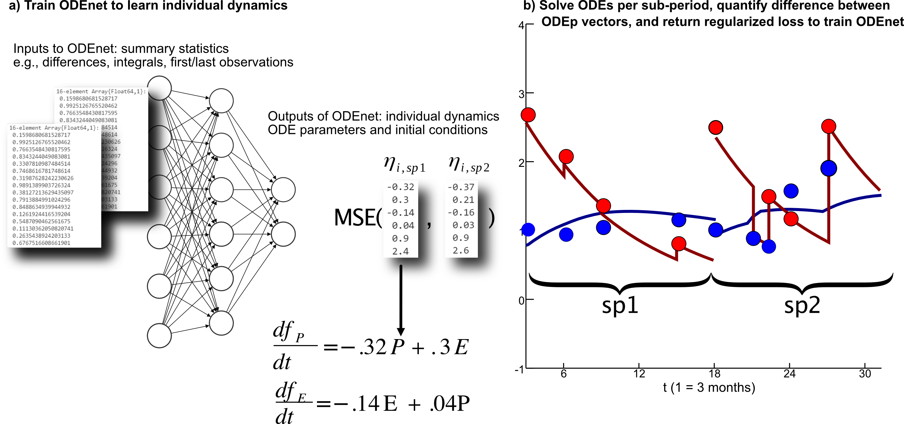
Figure 1: Overview of ODEnet extension for intra-individual learning of potentially changing dynamics. We parameterize our system of ordinary differential equations (ODEs) with a feed-forward neural network (ODEnet) which receives summary statistics of the respective sub-period (sp1 or sp2) as inputs. The critical advancement of our algorithm is the distinction and intra-individual coupling of sp1 and sp2 for each respondent. The mean squared error (MSE) of each intra-individual parameter set is summed, weighted by $\lambda_{sp}$, and provided as additional term to the loss function (see Equation (7)). Sp1 covers all observations T0–T6 from the baseline battery measurement (B0) to the repeated resilience factor testing battery (B1). Sp2 comprises all observations of mental health and stressor exposure after that.

We first provide a brief overview of the proposed approach, before subsequently describing its components in detail. A schematic illustration is given in Figure 1. VAEs are used for separate dimensionality reduction of mental health and stressor items. Longitudinal summary statistics of the time series of the resulting latent representation are fed into a second neural network—the ODEnet—which provides individual-level ODE parameters and their initial conditions (ICs) as output. The ODE parameters ($\eta_{i,1,sp},\ldots,\eta_{i,4,sp}$) and the ICs are obtained for each individual, separately for the two sub-periods. We introduce individual-level dependency by penalizing the difference of each ODE parameter between the sub-periods (but not the ICs). Thereby, the ODEnet is trained to find ODE parameters that best describe the dynamics of the respective sub-period and, at the same time, enforce some correlation between parameter sets from the same respondent, reflecting that the data is provided from the same respondent.

3.1 Dimensionality reduction per time point with VAEs

We choose Variational Autoencoders (VAEs; Kingma and Welling, 2019) to find lower-dimensional latent distributions $q_{\phi}(z|x)$ making use of variational inference (Blei et al., 2017). Let $x^{P}_{i}=(x^{P}_{i,1},\ldots,x^{P}_{i,p})$, be a vector of p items of P and $x^{E}_{i}=(x^{E}_{i,1},\ldots,x^{E}_{i,e})$ be a vector of e items of E and $i\in\{1,\ldots,N_{P}\}$ or $i\in\{1,\ldots,N_{E}\}$, respectively (see section 2). The latent variables of E or P are denoted as $z^{E}_{i}$ and $z^{P}_{i}$ for each realized observation $i$. Then, the VAEs are trained by maximizing the evidence lower bound (ELBO) of the marginal log-likelihood

$$\begin{split}\log p(x_{1},\ldots,x_{N})&=\sum_{i=1}^{N}\log p(x_{i})\\ &\geq\sum_{i=1}^{N}(\mathbb{E}_{q(z|x)}\log p(x_{i}|z)-\text{KL }(q(z|x_{i})||p(z)))\end{split}$$

where the first term of the right hand side is the expectation of the log-likelihood of $x_{i}$ given $z$ with respect to $q(z|x)$. The Kullback-Leibler divergence ($D_{KL}$) penalizes deviations of the posterior from the prior. Temporal dependence between the observations is established by the system of ODEs.

Intuitively, VAEs comprise an encoder and a decoder. The purpose of training the encoder (aka inference or recognition model) is to find good variational parameters $\phi$ that parameterize the distributions $q_{\phi}(z|x)$ in the latent space in a way, the decoder can reconstruct samples of that latent distribution that resemble the inputs $x_{i}$. In our case, the former is achieved by two separate EncoderNets

$$(\mu^{P}_{i},\log\sigma^{P}_{i}) =\text{EncoderNet}_{\phi_{P}}(x^{P}_{i})$$ (1)

$$(\mu^{E}_{i},\log\sigma^{E}_{i}) =\text{EncoderNet}_{\phi_{E}}(x^{E}_{i})$$ (2)

which yield the latent distributions

$$q_{\phi}(z^{P}_{i}|x^{P}_{i}) =\mathcal{N}(\mu^{P}_{i},\log\sigma^{P}_{i})$$ (3)

$$q_{\phi}(z^{E}_{i}|x^{E}_{i}) =\mathcal{N}(\mu^{E}_{i},\log\sigma^{E}_{i})$$ (4)

for each complete observation $i$. The two separate $\text{DecoderNets}(\theta)$ then take samples of $q_{\phi}(z|x)$ and are trained to increase the log-likelihood of the inputs given samples of the posterior distributions. Please note, while the expected value of the posterior distribution $\mu$ captures the position of the observation in the latent space, the variance $\sigma$ captures the uncertainty that is related to this mapping (see also Kingma and Welling, 2019).

For computation, we plug in the Poisson log-likelihood and the closed form of $D_{KL}$ for a Gaussian prior and posterior. Thereby, training objective of our VAEs become

$$\begin{split}\text{Loss}(\theta,\phi;x_{i})=&\underbrace{\frac{1}{2}\sum_{i=1}^{N}(1+\log((\sigma(x_{i}))^{2})-(\mu(x_{i}))^{2}-(\sigma(x_{i}))^{2})}_{D_{KL}(\phi)}+\\ &\underbrace{\sum_{i=1}^{N}(\lambda_{i}-x_{i}\times\log(\lambda_{i}))}_{\text{Poisson reconstruction error }(\theta)}+\\ &\underbrace{\lambda_{VAE}\times(\sum_{i}\phi+\sum_{i}\theta)}_{\text{Weight regularization}}\end{split}$$

where $\mu$ and $\sigma$ are the mean and standard deviation of the latent distribution depending on the observed values $x_{i}$. The expected value of the Poisson distribution of each item is denoted as $\lambda_{i}$ depending on the observation. To prevent overfitting, we regularized the encoder ($\phi$) and decoder ($\theta$) weights of both VAEs with $\lambda_{VAE}$.

The Poisson distribution does not perfectly match the MARP data since we find moderate levels of overdispersion for some items. Yet, the Poisson distribution avoids an additional parameter, which might be difficult to determine, by coupling the expected value and the dispersion. We used the $tanh$ activation functions in the middle layers. In the final layer, we used a $ReLU$ activation function to strictly pass non-negative values to $\lambda_{i}$.

3.2 ODEs to model the trajectories of E and P in the latent space

We use ODEs to couple the latent representations of P and E over time and allow for separate intra-individual parameter sets for periods between the resilience factor testing batteries (B0, B1), providing potential predictors of the individual dynamics. The exact design of such an ODE system is a crucial modeling decision since it governs how each component changes and requires domain expertise. We were able to model a slightly more complicated system of ODEs than Köber et al. (2020). Specifically, we use

$$\frac{df_{z^{P}_{i,t}}}{dt} =\eta_{i,1,sp}\times z^{P}_{i,t}+\eta_{i,2,sp}\times z^{E}_{i,t}$$ (5)

$$\frac{df_{z^{E}_{i,t}}}{dt} =\eta_{i,3,sp}\times z^{E}_{i,t}+\eta_{i,4,sp}\times z^{P}_{i,t}$$ (6)

where changes in $z^{P}_{i,t}$, the latent trajectory value of mental health problems (P) of respondent $i$ at $t$ with $i\in\{1,\ldots,N\}$ and $t\in\{1,\ldots,T\}$, and $z^{E}_{i,t}$, the latent trajectory value of stressors exposure (E), are driven by their own current value. Additionally, $z^{P}_{i,t}$ is allowed to change in response to $z^{E}_{i,t}$ and vice versa. Subscript $sp$ in $\eta_{i,1,sp}$ indicates that each individual set of parameters differs intra-individually between sp1 and sp2.

Negative values for $\eta_{i,1,sp}$ and $\eta_{i,3,sp}$ effectively realize system-inherent damping (Boker et al., 2010), where high E and P values are more quickly driven back to low values in the latent space. Thus, a high negative $\eta_{i,1,sp}$, in particular, reflects good recovery from mental health problems (since the majority of observations are mapped into the positive valued latent space or close to zero). This can be understood as one facet of stressor reactivity, where possible surges in mental health problems tend to be short-lasting. Positive values for $\eta_{i,2,sp}$ realize the adverse effect of E on P. A low positive $\eta_{i,2,sp}$ value thus reflects low responsivity of mental health to stressors in the first place, as the second element in our equation system that, overall, describes an individual’s stressor reactivity. $\eta_{i,4,sp}$ allows for the opposite direction and expresses that people with high P report more E in the future. This is deemed plausible, both because mental health problems are stressors in their own right that can induce further adverse reactions and because mentally ill persons may generate, or be confronted with, more conflicts or other types of adversities (Gerin et al., 2019). Key parameters, however, for the interpretation of an individual’s resilience status are $\eta_{i,1,sp}$ (recovery) and $\eta_{i,2,sp}$ (reactivity).

At each realized measurement of stressor exposure, its integrator $f_{z^{E}_{i}}$ is updated to the mapping of the actually observed values to the latent space $z^{E}_{i}$ at the precise point in (study) time when this observation was taken. This reflects the notion that stressor exposure levels are only partly driven by an endogenous property of the ODE system (i.e., damping and mental health) but mainly reflect exogenous forces, that is, the sudden occurrence or absence of stressors that lead to abrupt changes in the latent stressor values (see above).

The benefits of such an ODE system compared to discrete-time models like regression are crucial for analyzing the data from the MARP study. Most importantly, differential equations take all available information at the precise time into account. Thereby, irregular sampling intervals and entirely (or partly) missing observations are dealt with by the properties of our dynamical system (assuming non-informative missingness).

3.3 Finding individual and potentially changing ODE parameters with the ODEnet

The critical advancement of our method is the extension of the ODEnet to learn potentially changing ODE parameters $\eta_{i,s,sp}$. The key idea is depicted in Figure 1. The ODEnet is trained by minimizing the $\text{Loss}_{ODE}(\tau,\eta_{i,s,sp})$ and provides a two-element vector of ODE parameters, each of length $s\in\{1,\ldots,4\}$, for both sub-periods

$$\eta_{i,s,sp}=(\eta_{i,s,sp1},\eta_{i,s,sp2})=\text{ODEnet}_{\tau}(x^{P}_{i},x^{E}_{i})$$

with the observed items $x^{P}_{i}$ and $x^{E}_{i}$ as inputs and the trainable parameters $\tau$. The ODEnet internally calls the EncoderNet (see Equation 1 and 2) which maps the observed values into the latent space. Subsequently, we calculate several summary statistics of the intra-individual sub-period in the latent space (e.g., integrals, first and last observations, and differences; see Table 1 in Köber et al. (2020)). It was left to gradient descent to find a good combination of these summary statistics to minimize $\text{Loss}_{ODE}(\tau,\eta_{i,s,sp})$. All summary statistics are required to be computable with only two observations from P and E (which can be reported at any point in time, not necessarily during the same observation). The main purpose of the ODEnet is to minimize the sum of the squared difference of the trajectory $f_{z_{i}}(t,\eta_{i,s,sp})$ and the mean of the latent space distribution $\mu_{i}$ at the precise point in study time $t$ depending on period-specific individual ODE parameters $\eta_{i,s,sp}$. Accordingly, the training objective of the ODEnet is

$$\begin{split}\text{Loss}_{ODE}(\tau,\eta_{i,s,sp})=&\sum_{i=1}^{N}\sum_{t=1}^{T}(f_{z_{i}}(t,\eta_{i,s,sp})-\mu_{z_{i,t}})^{2}\quad+\\ &\lambda_{sp}\times\sum_{s=1}^{4}(\eta_{i,s,sp1}-\eta_{i,s,sp2})^{2}\quad+\\ &\lambda_{ODEp}\times\sum_{s=1}^{4}\eta_{i,s,sp}\ \quad+\\ &\lambda_{ODEnet}\times\sum_{i}\tau\text{.}\end{split}$$ (7)

Importantly, the period-specific individual parameter sets within $\eta_{i,s,sp}$ are tied together by penalizing the squared difference of the two parameter sets $\eta_{i,s,sp1}$ and $\eta_{i,s,sp2}$. This bond of ODE parameters across the sub-periods reflects their intra-individual dependence. Furthermore, this tying helps to prevent overfitting of the ODE parameters to a certain period with, e.g., only a few unusual measurements. The hyperparameter $\lambda_{sp}$ $\in\mathbb{R}_{>0}$ allows to tune the strength of this connection. We additionally penalize both the sum of the ODE parameters with $\lambda_{ODEp}$ as well as the weights of the ODEnet with $\lambda_{ODEnet}$ to avoid overfitting.

The concrete values of the hyperparameter $\lambda_{sp}$ can be decided based on subject-matter considerations, e.g., by imposing stronger similarity between intra-individual sub-period dynamics for subject areas which are known for evolving slowly, or by optimization criteria, e.g., cross-validated mean squared error (MSE) as usual in Lasso analyses (Hastie et al., 2015). Please note, the differences of the initial conditions (IC) are not penalized, although the ODEnet also provides them.

More detailed, the ODEnet is a three-layer feed-forward neural network. We use a $ReLU$ activation function in the middle layer and no transformation in the final layer. Using no activation function in the last layer does allow the ODEnet to find the parameters of the dynamical system freely; put differently, it enables the ODEnet to provide the full numerical range of possible ODE parameters. We increased the capacity of the ODEnet—the mid-layer has 12 nodes now—compared to Köber et al. (2020), mainly due to the increased number of training examples (with the additional split at the second lab visit, most respondents contributed two time series). Hyperparameter tuning on the empirical data with regularization and a simulation study agreed that this architecture balances bias and variance well. Learning the ICs overcomes the limitation of Köber et al. (2020), which regarded the first observation as ground truth.

To increase training stability, we initialized the ODEnet with very small weights and trained it rather slowly for 100 epochs with a small learning rate of $\alpha=10e^{-4}$. Furthermore, we scale the inputs to ensure approximately equal numerical size. Flexible dynamical modeling is provided by DifferentialEquations.jl (Rackauckas et al., 2019) and differentiable through neural nets via DiffEqFlux.jl (Rackauckas et al., 2019). To deal with unit non-response, $\text{Loss}(\theta,\phi;x,\lambda_{VAE})$ and $\text{Loss}_{ODE}(\tau,\eta_{i})$ are only evaluated at actual measurement time points. All neural networks were trained with Flux.jl (Innes et al., 2018) and the Adam optimizer (Kingma and Ba, 2014). We used this website (LeNail, 2019) as a basis for drawing the ODEnet in Figure 1.

3.4 A two-stage Lasso approach to repeated battery updates

We assess the capabilities of the incoming predictor information to improve the prediction beyond the older (but potentially still relevant) subject information with a variant of the Lasso tailored to this data situation. The particularity of this data is that an extensive (and expensive) multi-modal resilience factor testing battery including—next to questionnaires—also neuroimaging and biosampling, amongst others, is repeated in regular intervals (at B0, B1, …). In the meantime, several samples of key resilience outcome variables (mental health problems and stressor exposure) are drawn (at T0, T1, …). To be able to learn about the usefulness of the incoming testing battery information (B1) for prediction, we add an additional weight vector $w$ to the standard Lasso training criterion. The optimal parameters for all available battery information (B0 and B1) predicting the dynamics in the second sub-period (sp2) are

$$\hat{\beta}_{sp2}=\underset{\beta}{\operatorname{argmax}}\{\frac{1}{2}|y-X\times\beta|^{2}+\lambda_{\text{Lasso}}\sum^{p}_{j=1}w\times\beta\}$$

where $X$ is the design matrix, y is a resilience-related outcome, and $\lambda_{\text{Lasso}}$ is the penalty coefficient of the Lasso.

This approach has been already suggested for cross-sectional data settings before (Zou, 2006) and can be implemented simply using the established R package glmnet (Friedman et al., 2010); this circumstance fosters reusability of the approach, also independently of the estimation of dynamics with the ODEnet as suggested above. In the first step of our two-stage approach, the Lasso is trained only with predictor data of the initial baseline observation (B0) to predict the learned dynamics of the first sub-period. Since no previous knowledge is assumed, the penalty factor is set to its default ($w=1$) for all potential predictors. In a second step, both battery information from B0 and B1 provide potential predictors of the dynamics of the second sub-period (sp2). We use the previous Lasso analysis and penalize the initial data from B0 with $-\log(VIF)$ while we penalize incoming data uniformly with the default ($w=1$).

We use the variable inclusion frequencies ($VIF$) because single lasso analyses might be unstable regarding the selected variables. For this reason, Wallisch et al. (2021) suggest using resampling to determine model stability (see also Heinze et al. (2018) and Sauerbrei et al. (2015)). More precisely, we resampled a proportion of $m=0.8$ and repeated the Lasso analysis 1.000 times, using 6-fold cross-validation to determine the strength of the lasso penalty once.

More detailed, assuming that each testing battery (B0, B1, …) provides the same number of variables $v$, and that there are less individuals who met the minimum requirements, $N_{sp1}$ is usually larger than $N_{sp2}$. The $v\times n_{sp1}$ matrix $X_{sp1}$ of potential resilience factors is accompanied by the weight vector $w_{sp1}=(w_{sp1,1},\ldots,w_{sp1,v})=(1,\ldots,1)$ when predicting an indicator of the dynamics of the first sub-period $y_{sp1}$. For the second sub-period, however, we stack both baseline information on top of each other, accordingly, $X_{sp2}$ is $m\times n_{sp2}$ where $m=2\times v$ (in case $v_{sp1}=v_{sp2}$). The weight vector of the second sub-period can be expressed as

$$w_{sp2}=\left\{\begin{array}[]{lr}-\log(VIF(X_{r})),&\text{for }r\leq\frac{m}{2}\\ 1,&\text{for }r>\frac{m}{2}\\ \end{array}\right\}$$

with $r\in\{1,\ldots,p\}$.

We predict the ODE mental health responsivity parameter $\eta_{i,2,sp}$ which is a choice made for this paper, intending to demonstrate the method. One could also choose a different prediction target, e.g., $\eta_{i,1,sp}$ which reflects the recovery of mental health, or impose a considerable amount of stress on the entire individual dynamical system (or, more precisely, each learned parameter set $\eta_{i,s,sp}$ plugged into the shared dynamical system structure) and predict mental health at predefined time points (as done by Köber et al. (2020)), depending on which aspect one thinks is more interesting from a subject-matter perspective.

4 Results

First, we compare dynamical systems (see Equation (5)) of mental health problems (P, blue) and stressor exposure (E, red) of two exemplary individuals (rows) with different intra-individual difference penalization terms $\lambda_{sp}$ (columns; see Equation (7)) in Figure 2. As in Figure 1, the y-axis shows the position of P and E in the latent space, and the x-axis shows time (where one unit in x represents three months in study time). The expected values of the latent value distributions, learned by the VAEs, are expressed as dots. The trajectories, governed by the ODEs, are depicted as lines. Figure 2 exemplifies that this algorithm is able to detect potential sub-period differences and that $\lambda_{sp}$ can alter the strength of this difference (based on, e.g., subject-matter considerations or cross-validation).

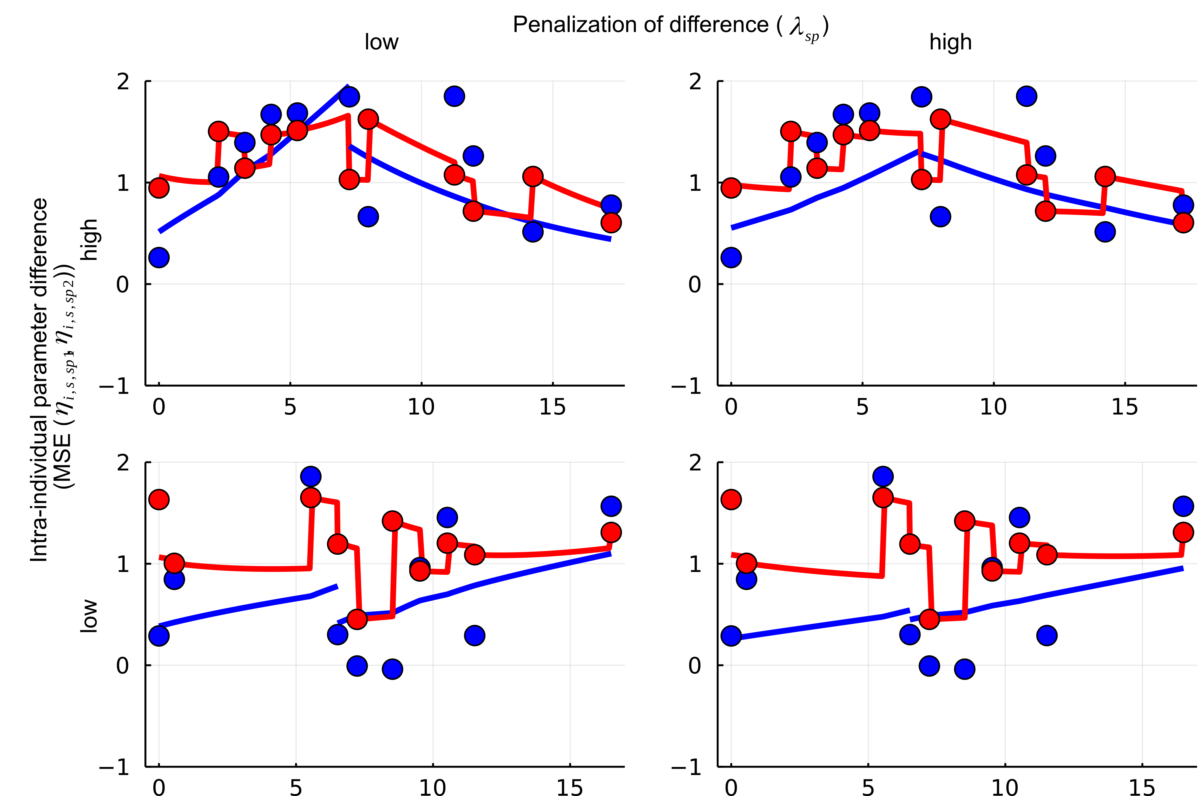
Figure 2: This figure shows an exemplary comparison of the differences between sub-periods of dynamical systems. Mental health problems (P, blue) and stressor exposure (E, red) are shown for two respondents (rows) with low ($\lambda_{sp}=0.4$) and high ($\lambda_{sp}=3.6$) values of intra-individual deviation penalty (columns). The upper row shows a respondent with considerable change in the ODE parameters between sub-period 1 to 2 (sp1 and sp2). P increase in sp1. In contrast, P decreases in sp2. This change is visibly mitigated, although still present, when the ODEnet is trained with a stronger penalization of parameter differences $\lambda_{sp}=3.6$ (right column). The second row shows a respondent with a low change in the ODE parameters. Accordingly, increasing $\lambda_{sp}$ (from left to right) does not affect the intra-individual comparison strongly.

Furthermore, this particular data situation allows us to investigate the practice-oriented question of which parts of the repeated battery are particularly worth updating. To illustrate this, we predict the ODE mental health responsivity parameter $\eta_{i,2,sp}$ directly—which captures how the level of stressor exposure influences the gradient of mental health problems—with a two-staged lasso approach (see the Methods section for more details) and show and discuss the results in Figure 3 with a heat map.

Please note that while only information of B0 is included in the analysis of sp1, variables of B0 and B1 are included in the analysis of sp2. However, due to the very low penalization weight $w$ of the frequently selected variables (and reversely the very high weight of the non-selected variables) they are almost certainly (not) selected, which renders their visualization pointless. Since variable selection approaches are known for being unstable, we choose VIF (Wallisch et al., 2021) for both as the decisive criterion for our two-staged procedure determining the weights and for visualizing the results.

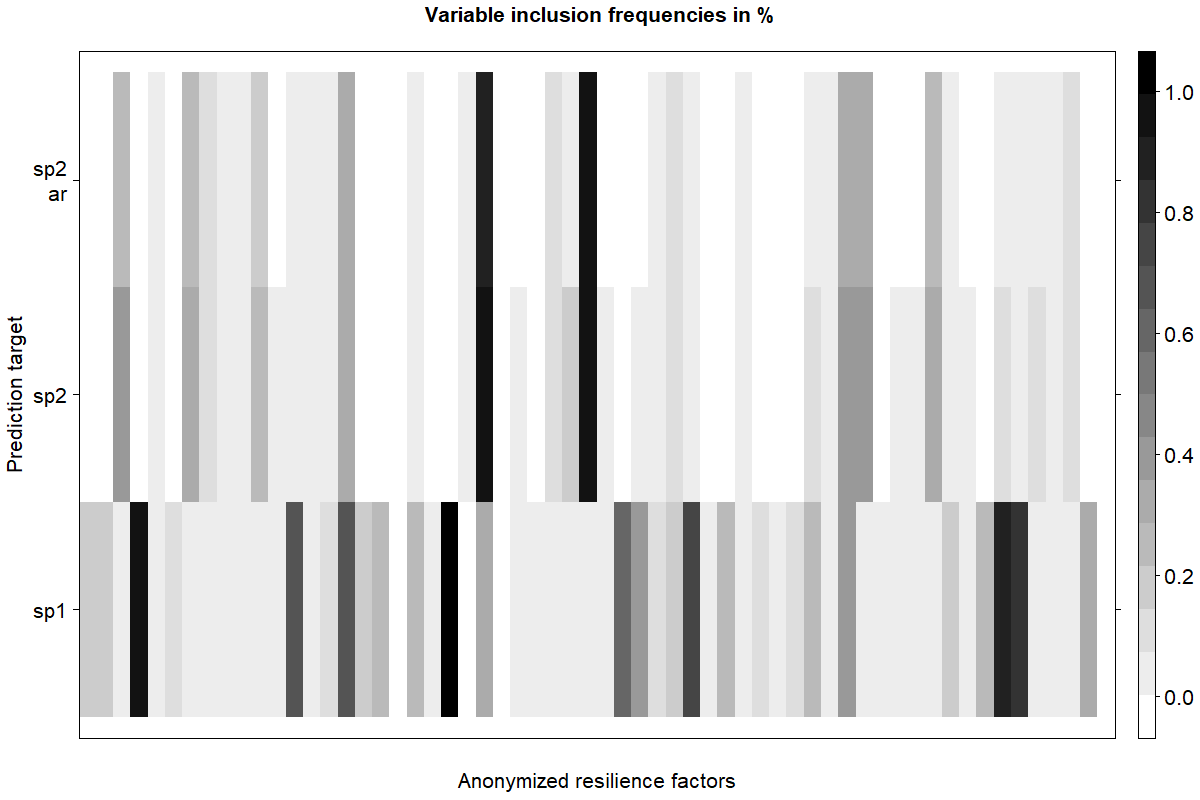
Figure 3: Variable inclusion frequencies (VIF) of the Lasso analysis with different prediction targets. This heat map provides insights into which battery measures (x-axis) predict the targets (y-axis) derived for this longitudinal focus. All rows of the y-axis depict the two sub-periods or, more precisely, $\eta_{i,2,sp1}$ and $\eta_{i,2,sp2}$ from the ODEs (see Equation (5)), which captures the individual gradient of mental health in response to stressor exposure in the dynamical system. Importantly, sp1 was predicted solely with B0 (initial lab visit at the beginning of the study). The second sub-period sp2 was predicted with both B0 and B1 (the latter is the first repetition of the initial lab visit’s testing battery around 1.75 years later), albeit with unequal penalty weights. This plot indicates that there are five stable and predictive variables in B0 (see lowest row) when predicting sp1. Due to their high VIF, these variables are penalized with zero/very small $w_{sp2}$ when predicting sp2 (see the dedicated Methods section for more details). Accordingly, they are almost certainly entailed in the prediction of sp2 dynamics as well. Therefore, in the two upper rows, we show only the B1 predictors. Regarding potential resilience factors in the second testing battery B1, there is a mixed picture. While updates of already picked variables are chosen rather seldom, other measures now play a more important role when predicting sp2. The upper row (sp2 ar, for autoregressive) includes $\eta_{i,2,sp1}$ as an additional predictor in the Lasso analysis. This mitigates the VIF only slightly, indicating a rather stable pattern of particularly valuable parameter updates in B1. We deliberately do not show or discuss the specific constructs that we found to predict the individual dynamics since we focus on methods development here.

A subsequent question is whether we can predict the changes of $\eta_{i,2,sp2}$ in an auto-regressive manner. Put differently, do the recommendations on promising parameter updates hold even when including $\eta_{i,2,sp1}$ into the Lasso? All findings are discussed in the figure captions.

5 Discussion

Recently, there have been several proposals for deep dynamic modeling, where differential equations are used on latent representations obtained by VAEs. Motivated by an application from psychological resilience research, we removed the assumption of constant dynamics throughout the whole study period, implicit in these approaches. Instead, we showed how individual-level dynamic models could be fitted for two individual sub-periods and introduced a dependency between by a penalization term, which made our approach feasible also for a dataset with relatively small number of individuals.

We then used regularized regression, specifically the Lasso approach, to identify potential resilience factors from a baseline battery and its follow-up update that could predict summary statistics obtained from individual resilience trajectories. Such a variable selection approach, e.g., allows pruning the battery for subsequent lab visits, thus potentially saving time and money. We find that five resilience factors in the initial testing battery are particularly promising for predicting the dynamics in the first sub-period. While we pick few variables from the second lab visit in the second sub-period again, we could identify a small set variables that could be recommended for update. This suggests that a dramatically reduced battery would be sufficient for this prediction task. This findings holds when explicitly predicting parameter changes with an auto-regressive approach.

To deal with a relatively small number of respondents, our model also made efficient use of the vast majority of training data to learn the lower-dimensional representations, trajectories, and predictors. In particular, we provided all measurement time points separately as observations to the VAEs, and did not attempt to fit more complex neural networks architectures with time structure, such as recurrent neural networks, as time structure is already covered by the ODEs. Such dynamic models at the heart of neural networks are known to reduce sample size requirements in deep learning algorithms drastically (Rackauckas et al., 2020).

We also had to take several additional countermeasures to reduce the data hunger of deep learning methods, such as coupling the expected value and dispersion parameter by assuming a Poisson distribution for the item data. Furthermore, we have trained our neural networks on all available data and did not reserve any test set to investigate the generalization error. Instead, the role of subsequent validation is provided by the prediction with the Lasso. Specifically, the argument is that we could not have identified characteristics that prediction resilience prediction targets of the dynamic modeling would not reflect true underlying structure. Our insights and approaches regarding the feasibility of deep learning approaches when facing moderate sample sizes may also be more generally helpful in other studies that want to use similarly sophisticated approaches but are in doubt of whether their sample size is sufficient.

References

- Blei et al. (2017) Blei, D. M., Kucukelbir, A., and McAuliffe, J. D. (2017). Variational inference: A review for statisticians. Journal of the American Statistical Association 112, 859–877.
- Boker et al. (2010) Boker, S. M., Montpetit, M. A., Hunter, M. D., and Bergeman, C. S. (2010). Modeling resilience with differential equations. In Individual pathways of change: Statistical models for analyzing learning and development. American Psychological Association, pages 183––206.
- Bonanno et al. (2011) Bonanno, G. A., Westphal, M., and Mancini, A. D. (2011). Resilience to loss and potential trauma. Annual Review of Clinical Psychology 7, 511–535.
- Bringmann et al. (2017) Bringmann, L. F., Hamaker, E. L., Vigo, D. E., Aubert, A., Borsboom, D., et al. (2017). Changing dynamics: Time-varying autoregressive models using generalized additive modeling. Psychological Methods 22, 409–425.
- Chen et al. (2018) Chen, T. Q., Rubanova, Y., Bettencourt, J., and Duvenaud, D. K. (2018). Neural Ordinary Differential Equations. In NeurIPS.
- Chmitorz et al. (2020) Chmitorz, A., Kurth, K., Mey, L. K., Wenzel, M., Lieb, K., et al. (2020). Assessment of Microstressors in Adults: Questionnaire Development and Ecological Validation of the Mainz Inventory of Microstressors. JMIR Mental Health 7.
- Driver and Voelkle (2018) Driver, C. C. and Voelkle, M. C. (2018). Hierarchical Bayesian continuous time dynamic modeling. Psychological Methods 23, 774–799.
- Esteva et al. (2017) Esteva, A., Kuprel, B., Novoa, R. A., Ko, J., Swetter, S. M., et al. (2017). Dermatologist-level classification of skin cancer with deep neural networks. Nature 542, 115–118.
- Friedman et al. (2010) Friedman, J., Hastie, T., and Tibshirani, R. (2010). Regularization Paths for Generalized Linear Models via Coordinate Descent. Journal of Statistical Software 33, 1–22.
- Gerin et al. (2019) Gerin, M. I., Viding, E., Pingault, J.-B., Puetz, V. B., Knodt, A. R., et al. (2019). Heightened amygdala reactivity and increased stress generation predict internalizing symptoms in adults following childhood maltreatment. Journal of child psychology and psychiatry 60, 752–761.
- Goldberg et al. (1997) Goldberg, D. P., Gater, R., Sartorius, N., Ustun, T. B., Piccinelli, M., et al. (1997). The validity of two versions of the GHQ in the WHO study of mental illness in general health care. Psychological Medicine 27, 191–197.
- Hackenberg et al. (2021) Hackenberg, M., Grodd, M., Kreutz, C., Fischer, M., Esins, J., et al. (2021). Using Differentiable Programming for Flexible Statistical Modeling. The American Statistician , 1–23.
- Hahn and Smith (1999) Hahn, S. E. and Smith, C. S. (1999). Daily hassles and chronic stressors: Conceptual and measurement issues. Stress Medicine 15, 89–101.
- Hastie et al. (2015) Hastie, T., Tibshirani, R., and Wainwright, M. (2015). Statistical learning with sparsity: the lasso and generalizations. Chapman and Hall/CRC.
- Heinze et al. (2018) Heinze, G., Wallisch, C., and Dunkler, D. (2018). Variable selection–A review and recommendations for the practicing statistician. Biometrical Journal 60, 431–449.
- Hong and Lian (2012) Hong, Z. and Lian, H. (2012). Time-varying coefficient estimation in differential equation models with noisy time-varying covariates. Journal of Multivariate Analysis 103, 58–67.
- Inan and Wang (2017) Inan, G. and Wang, L. (2017). PGEE: An R Package for Analysis of Longitudinal Data with High-Dimensional Covariates. The R Journal 9, 393–402.
- Innes et al. (2019) Innes, M., Edelman, A., Fischer, K., Rackauckas, C., Saba, E., et al. (2019). A Differentiable Programming System to Bridge Machine Learning and Scientific Computing URL http://arxiv.org/abs/1907.07587.
- Innes et al. (2018) Innes, M., Saba, E., Fischer, K., Gandhi, D., Rudilosso, M. C., et al. (2018). Fashionable Modelling with Flux URL http://arxiv.org/abs/1811.01457.
- Kalisch et al. (2017) Kalisch, R., Baker, D. G., Basten, U., Boks, M. P., Bonanno, G. A., et al. (2017). The resilience framework as a strategy to combat stress-related disorders. Nature Human Behaviour 1, 784.
- Kalisch et al. (2019) Kalisch, R., Cramer, A. O., Binder, H., Fritz, J., Leertouwer, I., et al. (2019). Deconstructing and reconstructing resilience: a dynamic network approach. Perspectives on Psychological Science 14, 765–777.
- Kalisch et al. (2021) Kalisch, R., Köber, G., Binder, H., Ahrens, K. F., Basten, U., et al. (2021). The Frequent Stressor and Mental Health Monitoring-Paradigm: A Proposal for the Operationalization and Measurement of Resilience and the Identification of Resilience Processes in Longitudinal Observational Studies. Frontiers in Psychology 12, 3377.
- Kampa et al. (2018) Kampa, M., Schick, A., Yuen, K., Sebastian, A., Chmitorz, A., et al. (2018). A Combined Behavioral and Neuroimaging Battery to Test Positive Appraisal Style Theory of Resilience in Longitudinal Studies URL https://www.biorxiv.org/content/early/2018/11/17/470435.
- Kidger et al. (2020) Kidger, P., Morrill, J., Foster, J., and Lyons, T. (2020). Neural Controlled Differential Equations for Irregular Time Series. URL https://arxiv.org/abs/2005.08926.
- Kingma and Ba (2014) Kingma, D. P. and Ba, J. (2014). Adam: A method for stochastic optimization URL http://arxiv.org/abs/1412.6980.
- Kingma and Welling (2013) Kingma, D. P. and Welling, M. (2013). Auto-encoding variational bayes URL http://arxiv.org/abs/1312.6114.
- Kingma and Welling (2019) Kingma, D. P. and Welling, M. (2019). An Introduction to Variational Autoencoders. Foundations and Trends® in Machine Learning 12, 307–392. URL http://dx.doi.org/10.1561/2200000056.
- Köber et al. (2020) Köber, G., Pooseh, S., Engen, H., Chmitorz, A., Kampa, M., et al. (2020). Individualizing deep dynamic models for psychological resilience data URL https://www.medrxiv.org/content/10.1101/2020.08.18.20177113v2.
- LeNail (2019) LeNail, A. (2019). Nn-svg: Publication-ready neural network architecture schematics. Journal of Open Source Software 4, 747.
- Meng et al. (2021) Meng, L., Zhang, J., Zhang, X., and Feng, G. (2021). Bayesian estimation of time-varying parameters in ordinary differential equation models with noisy time-varying covariates. Communications in Statistics - Simulation and Computation 50, 708–723.
- Montpetit et al. (2010) Montpetit, M. A., Bergeman, C. S., Deboeck, P. R., Tiberio, S. S., and Boker, S. M. (2010). Resilience-as-process: negative affect, stress, and coupled dynamical systems. Psychology and Aging 25, 631–640.
- Putter and van Houwelingen (2017) Putter, H. and van Houwelingen, H. C. (2017). Understanding landmarking and its relation with time-dependent Cox regression. Statistics in biosciences 9, 489–503.
- Rackauckas et al. (2019) Rackauckas, C., Innes, M., Ma, Y., Bettencourt, J., White, L., et al. (2019). DiffEqFlux.jl – A Julia Library for Neural Differential Equations URL http://arxiv.org/abs/1902.02376.
- Rackauckas et al. (2020) Rackauckas, C., Ma, Y., Martensen, J., Warner, C., Zubov, K., et al. (2020). Universal Differential Equations for Scientific Machine Learning. URL https://arxiv.org/abs/2001.04385.
- Refisch et al. (2021) Refisch, L., Lorenz, F., Riedlinger, T., Taubenböck, H., Fischer, M., et al. (2021). Data-Driven Prediction of COVID-19 Cases in Germany for Decision Making URL https://www.medrxiv.org/content/10.1101/2021.06.21.21257586v1.
- Rizopoulos (2012) Rizopoulos, D. (2012). Joint models for longitudinal and time-to-event data: With applications in R. CRC Press, Boca Raton, FL.
- Rubanova et al. (2019) Rubanova, Y., Chen, R. T. Q., and Duvenaud, D. (2019). Latent ODEs for Irregularly-Sampled Time Series. URL https://arxiv.org/abs/1907.03907.
- Sauerbrei et al. (2015) Sauerbrei, W., Buchholz, A., Boulesteix, A.-L., and Binder, H. (2015). On stability issues in deriving multivariable regression models. Biometrical Journal 57, 531–555.
- Schelldorfer et al. (2011) Schelldorfer, J., Bühlmann, P., and de Geer, S. v. (2011). Estimation for High-Dimensional Linear Mixed-Effects Models Using 11-Penalization. Scandinavian Journal of Statistics 38, 197–214.
- Schelldorfer et al. (2014) Schelldorfer, J., Meier, L., and Bühlmann, P. (2014). GLMMLasso: An Algorithm for High-Dimensional Generalized Linear Mixed Models Using 1-Penalization. Journal of Computational and Graphical Statistics 23, 460–477.
- Schmidtmann et al. (2014) Schmidtmann, I., Elsäßer, A., Weinmann, A., and Binder, H. (2014). Coupled variable selection for regression modeling of complex treatment patterns in a clinical cancer registry. Statistics in medicine 33, 5358–5370.
- Serido et al. (2004) Serido, J., Almeida, D. M., and Wethington, E. (2004). Chronic stressors and daily hassles: Unique and interactive relationships with psychological distress. Journal of Health and Social Behavior 45, 17–33.
- Wallisch et al. (2021) Wallisch, C., Dunkler, D., Rauch, G., de Bin, R., and Heinze, G. (2021). Selection of variables for multivariable models: Opportunities and limitations in quantifying model stability by resampling. Statistics in Medicine 40, 369–381.
- Wang et al. (2007) Wang, L., Chen, G., and Li, H. (2007). Group SCAD regression analysis for microarray time course gene expression data. Bioinformatics 23, 1486–1494.
- Wang et al. (2012) Wang, L., Zhou, J., and Qu, A. (2012). Penalized Generalized Estimating Equations for High-Dimensional Longitudinal Data Analysis. Biometrics 68, 353–360.
- Zöller et al. (2016) Zöller, D., Schmidtmann, I., Weinmann, A., Gerds, T. A., and Binder, H. (2016). Stagewise pseudo-value regression for time-varying effects on the cumulative incidence. Statistics in medicine 35, 1144–1158.
- Zou (2006) Zou, H. (2006). The adaptive lasso and its oracle properties. Journal of the American Statistical Association 101, 1418–1429.