Performance optimizations for porting the openQ^⋆D package to GPUs

Abstract

OpenQ^⋆D code has been used by the RC^⋆ collaboration for the generation of fully dynamical QCD+QED gauge configurations with C^⋆ boundary conditions. In this talk, optimization of solvers provided with the openQ^⋆D package relevant for porting the code on GPU-accelerated supercomputing platforms is discussed. We present the analysis of the current implementations of the GCR solver preconditioned with Schwarz alternating procedure for ill-conditioned Dirac-operators. With the goal of enabling support for GPUs from various vendors, a novel method of adaptive CPU/GPU-hybrid implementation is proposed.

1 Introduction

The advent of GPUs in modern supercomputers enables the path towards exascale computing, where the peak operations per second is around $10^{18}$ [1]. To reach such a peak performance is challenging and highly depends on the problem as well as the involved data types. Since lattice QFT calculations are bound by memory bandwidth and not by compute performance, one must think about how to reduce memory traffic in order to increase performance. For example, data types with smaller bit lengths can be considered.

The scope of this work is an analysis of the different solver algorithms used in the lattice QFT application openQ*D-1.1 [2]. This software package is used for the generation of fully dynamical QCD+QED gauge configurations with C^⋆ boundary conditions and $O(a)$-improved Wilson-fermions. Different aspects of the solvers are highlighted to find potential for improvement.

The analysis in this document is performed using Python-implementations of the examined kernels. This switch of programming language and philosophy enabled to run the kernels with simulated data types that are usually non-accessible within the native application without significant implementation effort.

2 Conjugate Gradient

The conjugate gradient kernel cgne() implements the algorithm already in mixed precision. The complete kernel was simulated using different data types – floats as well as posits. The simulated data types were binary64, binary32, tensorfloat32, binary16, bfloat16, posit32, posit16, and posit8 (please refer to table 1 for more information on these formats). The considered Dirac-operator represented as a CSR-matrix had approximately 2% non-zero values.

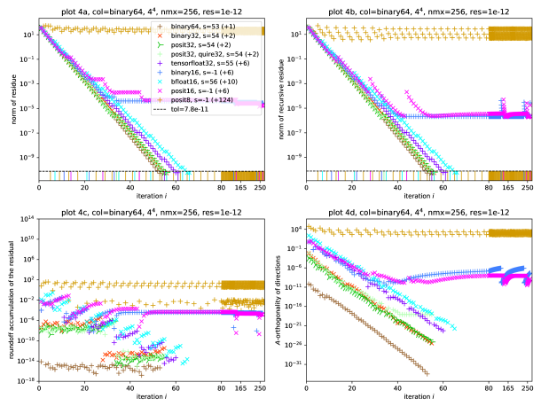
Figure 1: Convergence analysis of a conjugate gradient run, where binary32 was replaced by one of the simulated data types. The number s describes the number of regular CG-steps needed (the value of status), while the number in the brackets indicate the number of reset steps. Plot 4a shows the exact residue, $\vec{r}_{i}=\vec{b}-A\vec{x}_{i}$, calculated in every iteration in binary64, while plot 4b shows the norm of the recursively calculated residue, $\vec{r}_{i}=\vec{r}_{i-1}+\alpha_{i-1}A\vec{p}_{i-1}$, (cast to binary64 after calculation). The algorithm executes reset steps when the residue is lowered by an amount roughly the machine epsilon of the datatype (cf. table 1). These are indicated at the bottom of the plot. The relative residue suffers from round-off accumulation because of its recursive calculation; this is the difference between the two residues in plots 4a and 4b, which is plotted in plot 4c. Plot 4d shows the $A$-orthogonality of the current direction with respect to the last direction, namely the value of $\vec{p}_{i-1}^{\dagger}A\vec{p}_{i}$. The value of res – the desired relative residue of the calculated solution – is set to $10^{-12}$.

Figure 1 shows all the simulated data types using a reduction data type of binary64, meaning that all reduction operations where conducted in binary64. The following hierarchy is expected (smaller means convergence in fewer steps):

$${\color[rgb]{0.6015625,0.3984375,0.19921875}\text{binary64}}<{\color[rgb]{0,0.75,0}\text{posit32}}\leq{\color[rgb]{1,0.25,0}\text{binary32}}\leq{\color[rgb]{0.5,0,1}\text{tensorfloat32}}\leq{\color[rgb]{0,1,1}\text{(1)}}\leq{\color[rgb]{1,0,1}\text{posit16}}\leq{\color[rgb]{0.25,0.5,1}\text{binary16}}\leq{\color[rgb]{0,1,1}\text{(2)}}<{\color[rgb]{0.8203125,0.6015625,0}\text{posit8}},$$ (1)

where bfloat16 could be either at position (1) or (2), depending on what is more important; precision or number range.

Notice that hte target relative residual, $10^{-12}$, is outside the representable number range of binary16, posit16 and posit8. These data types cannot reach the target tolerance, therefore we didn’t expect them to converge. This is indeed the case. Furthermore, we see that binary16 and posit16 both are not able to go below $10^{-5}$, leading to no further considerable progress after step 45. This can be seen by the recursive residue stalling or even increasing – an indicator that the data type has reached its limits.

Both, binary32 and posit32, required the same number of steps, although round-off accumulation and $A$-orthogonality are slightly better for posit32. The reason for this is due to the higher density of posits in the relevant number regime (between $-1$ and $1$) leading to higher precision.

Finally, we compare the three data types with the same exponent range, but different precisions; binary32, tensorfloat32 and bfloat16 (cf. table 1). The less precision, the slower the convergence. The price to go from 23 to 10 mantissa bits results in 1 more conjugate gradient step as well as 4 more reset steps. When going further down to 7 mantissa bits again 1 more regular step and 4 more reset steps where needed to finally bring bfloat16 to convergence after 56 regular plus 10 reset steps. Bearing in mind that it occupies only 16 bits, this is a remarkable result, way better than its 16-bit competitors.

As seen in plot 4a, all data types start to converge by the same speed (all slopes are equal). The least precise data type, namely bfloat16 with its 7 mantissa bits, resets first, followed by binary16 and tensorfloat32, both with 10 mantissa bits. The next one is posit16, because it has more precision than binary16 in the relevant regime, followed by binary32 with 23 mantissa bits and later by posit32, where the same argument as before holds. The curve of binary64 would also reset at some point, but that never triggered in this run.

Specially plot 4a suggests that we can start to calculate in a data type with 16 bits of length until we fall below a constant value (proportional to the machine epsilon), then continuing the calculation in a data type with 32 bit-length until that number regime is exhausted as well, again switching to a 64 bit data type to finish the calculation.

2.1 Preliminary conclusions for the CG solver

Reduction variables should be chosen in a data type with large precision and number range, such as binary64, regardless of the current data type, since type conversions between different IEEE floating-point types are not considered to be expensive. On the other hand, the number of variables needed in that data type does not scale with the problem size or the number of steps, we can use a data type with large bit-length such as binary64.

The difference between tensorfloat32, binary32 and bfloat16 answers the question how important precision is in the calculation. The only relevant difference was in the number of reset steps. If the data type is lower in bit-length, the memory-boundedness of the problem suggests that the calculation performs faster. The trade-off is the amount of (computationally more expensive) reset steps that increase with lower precision.

Floating-point format limits
data type	$f_{max}$	$f_{min}$	$f_{smin}$	sign. digits	machine $\epsilon$
binary64 (e=11, m=52)	$1.79769313486231570\text{\times}{10}^{308}$	$2.22507385850720138\text{\times}{10}^{-308}$	$4.94065645841246544\text{\times}{10}^{-324}$	$\leq 15.9$	$2.2204460492503131\text{\times}{10}^{-16}$
binary32 (e=8, m=23)	$3.402823466\text{\times}{10}^{38}$	$1.175494350\text{\times}{10}^{-38}$	$1.401298464\text{\times}{10}^{-45}$	$\leq 7.2$	$1.1920928955078125\text{\times}{10}^{-07}$
binary16 (e=5, m=10)	$65504$	$0.00006103515625$	$5.9604644625\text{\times}{10}^{-8}$	$\leq 3.3$	$0.0009765625$
bfloat16 (e=8, m=7)	$3.38953138\text{\times}{10}^{38}$	$1.175494350\text{\times}{10}^{-38}$	$9.18354961\text{\times}{10}^{-41}$	$\leq 2.4$	$0.0078125$
tfloat32 (e=8, m=10)	$3.40116213\text{\times}{10}^{38}$	$1.175494350\text{\times}{10}^{-38}$	$1.14794370\text{\times}{10}^{-41}$	$\leq 7.2$	$0.0009765625$
posit32 (es=2)	$1.32922799578491587290\text{\times}{10}^{36}$	$7.52316384526264005099\text{\times}{10}^{-37}$	N/A	$\leq 8.1$	$7.450580596923828\text{\times}{10}^{-09}$
posit16 (es=1)	$2.68435456\text{\times}{10}^{8}$	$3.72529029\text{\times}{10}^{-9}$	N/A	$\leq 3.6$	$0.000244140625$
posit8 (es=0)	$64$	$0.015625$	N/A	$\leq 1.5$	$0.03125$

Table 1: Summary of highest representable numbers, $f_{max}$, minimal subnormal, $f_{smin}$, and non-subnormal, $f_{min}$, representable numbers above 0 in any common IEEE 754 floating-point and posit format [3, 4, 5, 6] together with their approximated precision in decimal. $e$ and $m$ denote the number of exponent and mantissa bits for floats, whereas $es$ denotes the maximal number of exponent bits for posits.

3 Schwarz Alternating Procedure

Domain decomposition is a way to partition the large system into (possibly many) smaller sub-problems with regularly updated boundary conditions coming from solutions of neighbouring sub-problems. They fit well into the notion of parallel processing because the sub-problem can be chosen to be contained in one single rank. The full lattice is split into sub-lattices called local lattice. Each rank has its own local lattice, the size of which is determined at compilation time. The full lattice consists of the ensemble of all local lattices arranged in a grid. These local lattices can be split as well into blocks. It is therefore advisable to choose the size of the blocks as divisor of the local lattice size such that one or more blocks fit into one rank. These sub-problems can then be solved using an iterative solving method.

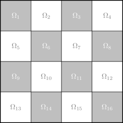
Figure 2: A $d=2$ dimensional example of a decomposition of a lattice $\Omega=\bigcup_{i=1}^{n}\Omega_{i}$ into $n=16$ domains named $\Omega_{i}$. Notice such a decomposition can always be colored like a chessboard.

The idea behind Schwarz Alternating Procedure (SAP) is to loop through all blocks $\Omega_{i}$ and solve the smaller sub-problem using boundary conditions given from the most recent global solution (cf. figure 2). If the original problem only includes nearest-neighbour interactions, the solution of a block $\Omega_{i}$ depends only on that block and its exterior boundary points, which are the adjacent points on the neighbouring blocks with opposite color. For example, the solution of the sub-problem involving $\Omega_{6}$, depends only on the solutions of $\Omega_{2}$, $\Omega_{5}$, $\Omega_{7}$ and $\Omega_{10}$. Therefore, all grey (white) blocks can be solved simultaneously, with the most recent boundary conditions obtained from the white (grey) blocks. Solving all grey, followed by all white blocks is called a Schwarz-cycle and is considered one iteration in SAP. Each block can be solved with any desired solver separately.

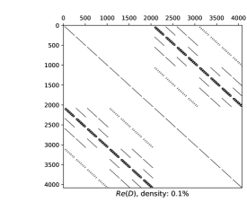
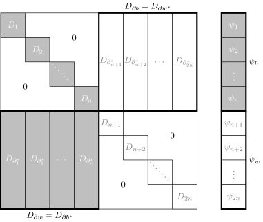
Figure 3: Left: An example plot of a Dirac-matrix of an $8^{4}$-lattice with SF-boundary conditions. The operator is already in a shape, where the even lattice points come first, followed by the odd lattice points. Every pixel consists of $192\times 192$ real numbers. White pixels denote zero, black pixels non-zero. Right: Schematic of the Dirac-operator in terms of a large sparse matrix. If the components of the black blocks are arranged such that they appear first, then the decomposition from figure 2 can be translated into a matrix with blocks as in the picture. $D_{i}$ describes the Dirac-operator restricted to block $i$ and $D_{\partial b}$ ($D_{\partial w}$) is the Dirac-operator restricted to the external boundaries of the black (white) blocks. The color external boundary operators can be decomposed into external boundary operators of the $i$-th block, $D_{\partial^{*}_{i}}$. The right side describes a vector decomposed into the same $2n$ domains $\psi_{1},\dots,\psi_{2n}$. The upper half corresponds to the black blocks and the lower half to the white blocks.

Whereas the division into domains on the lattice is straightforward, the representation of the Dirac-operator as a sparse matrix and its decomposition is not. Looking at an actual example of a Dirac-operator written as a matrix (cf. figure 3 left), one observes a lot of structure: while on the diagonal we find the operators restricted to the black and white blocks, the first and the third quadrant describe the operators restricted to the interior and exterior boundaries. The decomposition into $2n$ domains ($n$ grey and $n$ white blocks) can be translated as seen in figure 3 right. Notice that the restricted operators $D_{i}$ are easily solved, because they have block diagonal form.

3.1 Setup

The complete SAP+GCR kernel was implemented using Python in the same way as the fgcr() function from the source code. The Python implementation allowed a floating-point data type for the reduction variables separately (rdtype). It also accepts a "large" data type (ldtype) by which the restart steps are calculated in, and a "small" data type (sdtype) in which the regular and the MR steps are performed in. The result is obtained in terms of the "large" data type. There are various configuration settings to choose from (cf. table 2).

setting	meaning
res	desired relative residual
nmx	maximal number of GCR steps
nkv	number of generated Krylov vectors until restarting the algorithm
ncy	number of SAP-cycles to perform in each iteration
nmr	number of MR-steps to perform on each block in each SAP-cycle
bs	block size
ldtype	"large" data type
rdtype	reduction data type
sdtype	"small" data type

Table 2: Settings for SAP+GCR and their meanings.

The possible data types for ldtype, rdtype and sdtype are binary64 and binary32.

For the operator in figure 4, we see that preconditioning gives no significant improvement. This shows that for well-conditioned operators, too much preconditioning worsens the performance. $(n_{cy},n_{mr})=(1,4)$ is the configuration with the least amount of preconditioning. The CPU run-time shows a strong dependence on the configuration; there are even certain exceptional configurations, eg. $(12,2)$, that are more than $40$ times slower than the non-preconditioning case $(0,0)$. An unsuitable choice of configuration parameters can thus lead to a significant performance degradation. However, the plots show that performance of the algorithm is overly sensitive to the choice of these parameters. The adaptive variant might be of advantage here (cf. section 3.2).

The operator in figure 5 was at the critical point $k=k_{c}$. This is the regime where SAP-preconditioning shows its true potential; nearly all cases performed better than the trivial case. For the pure-CPU cases, we see no strong dependence on the amount of preconditioning, but on the block size. Small block sizes seem to be beneficial, while the pure-GPU variant prefers large block sizes. The hybrid cases – as usual in-between – are closer to the pure-GPU ones, because despite being hybrid most of the work is done on the GPU. The pattern within a certain block size is repeating and the best amount of preconditioning seems to be at $(4,6)$.

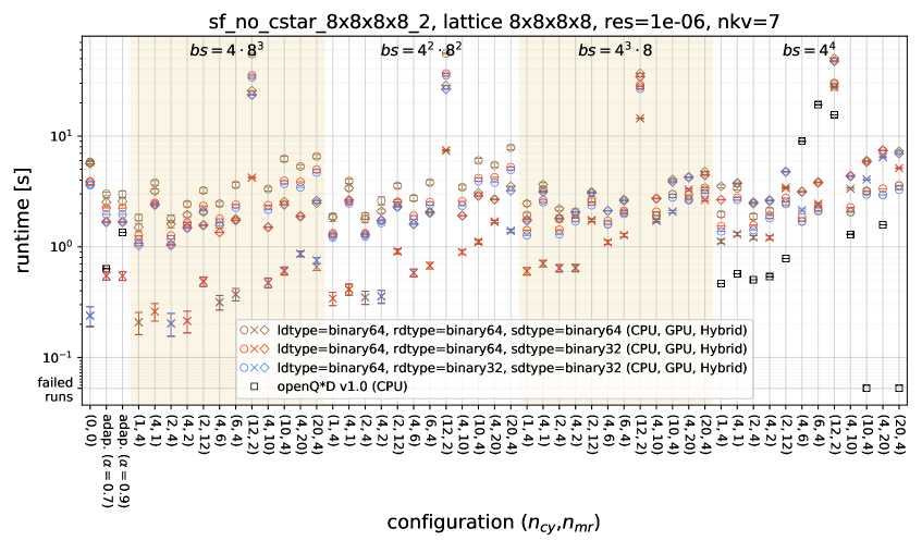
Figure 4: Time measurements for the SAP_GCR kernel on different matrices and configurations. The measurements were conducted on an Intel(R) 6130 @ 2.10GHz with 1.5 TB memory and an NVIDIA V100 (via PCIe) GPU with 16 GB memory. The x-axis gives the configuration in terms of $(n_{cy},n_{mr})$, the alternating shaded regions give the block size, whereas the shape of the data points indicate the processing device; circle, cross, diamond = pure CPU, pure GPU, Hybrid. Hybrid means that only the blocked problems where solved on the GPU.

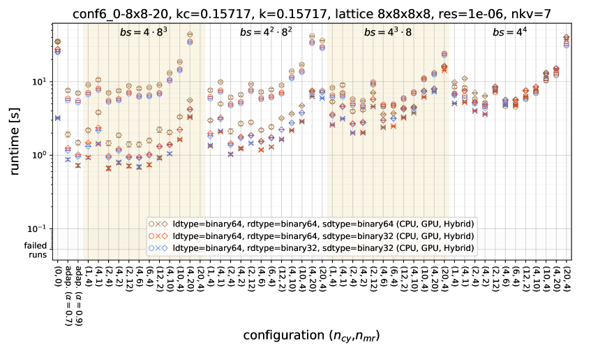
Figure 5: Time measurements for the SAP_GCR kernel on different matrices and configurations. The measurements were conducted on an AMD EPYC 7742 CPU @ 2.25GHz with 512 GB memory and an NVIDIA A100 (via SXM4) GPU with 40 GB memory. See figure 4 for more information.

Since the algorithm is applied to many different Dirac-operators among evolving HMC-trajectories – some well-conditioned, some ill-conditioned – it can be hard or even impossible to choose a set of parameters suitable for all cases. In particular, it is unavoidable to accidentally make a choice that falls on a configuration with exceptional long convergence time for a certain Dirac-operator within the long running HMC-simulation. It is therefore advisable to have the possibility to change the parameters during an active run or a configuration that adapts. This motivates the following proposal.

3.2 Proposal for an adaptive variant of SAP+GCR

Since the choice of parameters in the SAP+GCR kernel seems non-trivial, we propose an adaptive variant of this algorithm. In this version, the interpretation of the two parameters $n_{cy}$, $n_{mr}$ from table 2 is slightly different; they now denote the maximal amount of Schwart-cycles and MR-steps, respectively. The actual $n_{cy}$, $n_{mr}$ were chosen automatically in every iteration anew. They were determined as follows: If – after a Schwarz-cycle – the norm of the residual is not lower than the residual norm before the cycle, the preconditioning phase ends. Thus, at least one Schwarz-cycle is performed in every step. A similar, but slightly more complicated strategy is applied to determine the number of MR-steps. There are $3$ exit conditions for the MR-solver:

1. If – after at least $4$ MR-steps – the norm of the residual on the block is larger than $\alpha=0.9$ times the previous residual norm, the MR-solver exits, and the application continues processing the next block.

2. If the norm of the blocked residual becomes larger than the previous residual norm, the solver exits immediately, even if only one MR-step is executed.

3. If the norm of the blocked residual is smaller than the tolerance, the algorithm exit immediately too.

Every block is treated differently in every cycle. A maximum of $20$ Schwarz-cycles and $20$ MR-steps on each block would be performed if the above exit conditions never kick in. The third exit condition above makes sure to not overshoot the mark if the algorithm performs a lot of Schwarz-cycles and MR-steps, i.e. if the problem is already solved while in the preconditioning phase. This can happen if the operator is very well-conditioned or in the very last GCR-step before converging to the desired relative residual. Therefore, the adaptive version tries to find the optimal configuration for every iteration of the GCR-solver, for every Schwarz-cycle and for every block separately. By empirical observation of the results, the adaptive variant usually performs nearly maximal amounts of preconditioning in the first few GCR-steps, then rapidly decreases after some steps and finally saturate to the minimal amount that stays until convergence.

The results on how this adaptive variant competes with static configurations can be seen in the figures indicated by a configuration $\text{adap. }(\alpha=0.9)$ and $\text{adap. }(\alpha=0.7)$. Although the adaptive variant of the algorithm is not the fastest among all configurations, the plots show that it is certainly the most versatile one. It can be of benefit if the condition of the operator is not known beforehand and might even change drastically within a long running simulation.

A reference implementation has been added to openQ^⋆D and can be found in the GitLab repository ref. [8].

References

- [1] “Top 500: The List..” https://www.top500.org/.
- [2] I. Campos, P. Fritzsch, M. Hansen, M. K. Marinkovic, A. Patella, A. Ramos, and N. Tantalo, “openQ*D code: a versatile tool for QCD+QED simulations,” The European Physical Journal C, vol. 80, no. 3, pp. 1–24, 2020. Accessed: 2021-01-06.
- [3] Institute of Electrical and Electronics Engineers. Computer Society. Standards Committee and Stevenson, David, IEEE standard for binary floating-point arithmetic. IEEE, 1985.
- [4] S. Wang and P. Kanwar, “Bfloat16: the secret to high performance on cloud TPUs,” Google Cloud Blog, 2019.
- [5] R. Krashinsky, O. Giroux, S. Jones, N. Stam, and S. Ramaswamy, “NVIDIA ampere architecture in-depth,” NVIDIA blog: https://devblogs. nvidia. com/nvidia-ampere-architecture-in-depth, 2020.
- [6] P. W. Group et al., “Posit standard documentation - Release 3.2-draft,” Posit Standard Documentation, 2018.
- [7] R. Okuta, Y. Unno, D. Nishino, S. Hido, and C. Loomis, “CuPy: A NumPy-Compatible Library for NVIDIA GPU Calculations,” in Proceedings of Workshop on Machine Learning Systems (LearningSys) in The Thirty-first Annual Conference on Neural Information Processing Systems (NIPS), 2017.
- [8] R. Gruber, “Adaptive branch in GitLab repository: adaptive implementation SAP+GCR.” https://gitlab.com/roman.gruber/openQxD/-/tree/adaptive_sap_gcr, 2021.