Phase Vocoder Done Right

Abstract

The phase vocoder (PV) is a widely spread technique for processing audio signals. It employs a short-time Fourier transform (STFT) analysis-modify-synthesis loop and is typically used for time-scaling of signals by means of using different time steps for STFT analysis and synthesis. The main challenge of PV used for that purpose is the correction of the STFT phase. In this paper, we introduce a novel method for phase correction based on phase gradient estimation and its integration. The method does not require explicit peak picking and tracking nor does it require detection of transients and their separate treatment. Yet, the method does not suffer from the typical phase vocoder artifacts even for extreme time stretching factors.

I Introduction

The term phase vocoder was coined by Flanagan and Golden [1] but the now classical form of PV employing STFT analysis and synthesis using different analysis and synthesis steps for the purposes of time-scaling was introduced later by Portnoff [2, Sec. 6.4.4]. The way how the phase is corrected in the classical PV is based on the linear phase progression of a sinusoid with constant frequency. Each frequency channel is treated as a separate sinusoid whose phase is computed by accumulating the estimate of its instantaneous frequency and thus preserving the horizontal phase coherence [3]. Obviously, such an approach cannot cope well with time-varying sinusoidal signals and non-sinusoidal signals. A modification of PV was proposed by Laroche and Dolson [4, 5]. This improved PV involves spectral peak picking, tracking and “locking” the phase of the frequency bins belonging to a sinusoid to the phase of the peak (scaled phase locking). The phase locking enforces vertical phase coherence within the region of influence of the peak. Although the phase-locked PV is able to handle signals consisting of sinusoids with time-varying frequencies, it still fails for percussive sounds and transient events in general. A review of the phase vocoder, its history and alternative approaches to time and frequency scale modifications of audio signals can be found in [6, 7, 8].

Time scaling using phase vocoder techniques is known to produce specific artifacts such as transient smearing, “echo” and “loss of presence” collectively referred to as phasiness [4]. The artifacts are generally attributed to the loss of vertical phase coherence. Transient smearing compensation has been addressed by several authors. The most common approach is performing a phase reset or phase locking at transients [9, 10, 11]. Other approaches involve disabling the time-scaling at transients [12], or rely on using different window lengths for harmonic and transient parts [13, 14]. All approaches mentioned rely on correct transient detection. The preservation of vertical phase coherence is considered to be important for the quality of time-scaled voiced speech signals. It has been reported that not preserving the relative phase shift between the fundamental and the partials is perceived as unnatural. Several specialized methods for time-stretching of monophonic voice signals were proposed [15, 16]. Historically, time scaling techniques which preserve relative phase shift between the partials are called shape preserving [17]. To avoid dealing with phase altogether, a magnitude-only reconstruction has been considered [18]. Although efficient and real-time algorithms have recently been proposed, e.g. [19, 20], they do not perform favorably for large stretching factors. This is due to the magnitude not complying with the new synthesis step.

In this paper, we propose a novel method for phase correction in the PV, relying on both partial derivatives of the STFT phase and their integration. The phase derivatives are estimated using centered finite differences and the integration is performed through real-time phase gradient heap integration algorithm (RTPGHI) [19], an extension of the PGHI algorithm [21], originally proposed for magnitude-only reconstruction. The algorithm automatically enforces horizontal and vertical phase coherence even for broadband, non-sinusoidal components. No explicit peak picking or transient detection is required.

II Classical PV Revisited

In this section, we recall the essential formulas connected to PV and explain the role of the partial STFT phase derivative in the time direction. We further show with a straightforward example, that the poor performance of the classical PV for non-sinusoidal components can be attributed to neglecting the frequency direction partial phase derivative.

Given a discrete time signal $f$ which is nonzero on the interval $0,\dots,L-1$, a real-valued analysis window $g_{\text{a}}$ concentrated around the origin and the analysis time step $a_{\text{a}}$, the discrete STFT is given by

$$c(m,n)=\sum_{l\in\mathbb{Z}}f(l+na_{\text{a}})g_{\text{a}}(l)\mathrm{e}^{-\mathrm{i}2\pi ml/M}$$ (1)

for $m=0,\dots,M-1$, $M$ being the FFT length, and $n=0,\dots,N-1$, where $N=L/a_{\text{a}}$ is the number of STFT frames. Setting $M=L$ results in the full frequency resolution, but, typically, it is chosen such that $M\ll L$. We define the analysis frequency step as

$$b_{\text{a}}=\frac{L}{M}.$$ (2)

The magnitude $s$ and phase $\phi_{\text{a}}$ components of the STFT can be separated by

$$s(m,n) =\left|c(m,n)\right|,$$ (3)

$$\phi_{\text{a}}(m,n) =\arg\left(c(m,n)\right).$$ (4)

The time scaling factor will be defined as

$$\alpha=\frac{a_{\text{s}}}{a_{\text{a}}},$$ (5)

where $a_{\text{s}}$ denotes the synthesis time step. The length of the output signal is therefore equal to $\alpha L$ and the synthesis frequency step to

$$b_{\text{s}}=\alpha{b_{\text{a}}}.$$ (6)

The synthesis phase is constructed by the recursive phase propagation (integration) formula [5]

$$\phi_{\text{s}}(m,n)=\phi_{\text{s}}(m,n-1)+a_{\text{s}}\left(\Delta_{\text{t}}\phi_{\text{a}}\right)(m,n),$$ (7)

where $\Delta_{\text{t}}$ performs differentiation of the analysis phase $\phi_{\text{a}}$ (see Section III for details), or alternatively, by employing the trapezoidal integration rule, by

$$\begin{split}\phi_{\text{s}}(m,n)&=\phi_{\text{s}}(m,n-1)+{}\\ &+\frac{a_{\text{s}}}{2}\left(\left(\Delta_{\text{t}}\phi_{\text{a}}\right)(m,n-1)+\left(\Delta_{\text{t}}\phi_{\text{a}}\right)(m,n)\right).\end{split}$$ (8)

The time-scaled signal $\widetilde{f}$ is reconstructed using

$$\widetilde{f}(l) =\sum_{n=0}^{N-1}\widetilde{f_{n}}(l-na_{\text{s}})\ \ \ \text{for}\ l=0,\dots,\alpha L-1\ \text{with}$$ (9)

$$\widetilde{f_{n}}(l) =g_{\text{s}}(l)\sum\limits_{m=0}^{M-1}s(m,n)\mathrm{e}^{\mathrm{i}\phi_{\text{s}}(m,n)}\mathrm{e}^{\mathrm{i}2\pi ml/M}\ \ \text{and with}$$ (10)

$$g_{\text{s}}(l) =\frac{1}{M}\frac{g_{\text{a}}(l)}{\sum_{n\in\mathbb{Z}}g_{\text{a}}(l-na_{\text{s}})^{2}}$$ (11)

being the synthesis window $g_{\text{s}}$. To summarize, the classical PV performs differentiation and back integration of the phase in the time direction for all frequency bins.

Formula (1) can be interpreted as a sampling of the continuous STFT which is by itself a two-dimensional function of time and frequency. Therefore, $\left(\Delta_{\text{t}}\phi_{\text{a}}\right)$ can be interpreted as an approximation of the partial derivative of the phase in time. The complete phase gradient however involves also the partial derivative in frequency whose approximation will further be denoted as $\left(\Delta_{\text{f}}\phi_{\text{a}}\right)$. This second gradient component is completely disregarded in the classical PV, which introduces significant inaccuracies except for pure, stationary sinusoids. For the latter, $\left(\Delta_{\text{f}}\phi_{\text{a}}\right)$ indeed equals zero. The example in Figures 1A–1C shows plots of a spectrogram of a sum of a pure sinusoid, an exponential chirp and an impulse and of the partial derivatives of the phase. In particular, Figure 1C shows that, for the chirp and pulse components, $\left(\Delta_{\text{f}}\phi_{\text{a}}\right)$ unsurprisingly has non-negligible values.

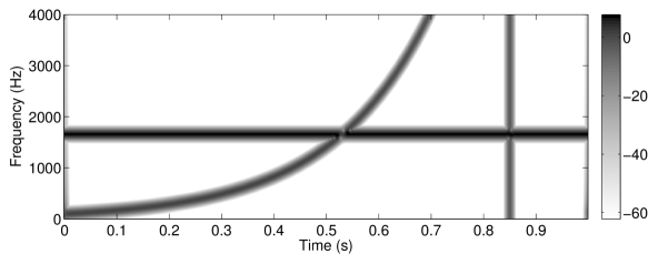
(Figure 1A) Spectrogram of a sum of a pure sinusoid, an exponential chirp and an impulse. The values are in dB.

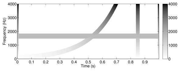
(Figure 1B)

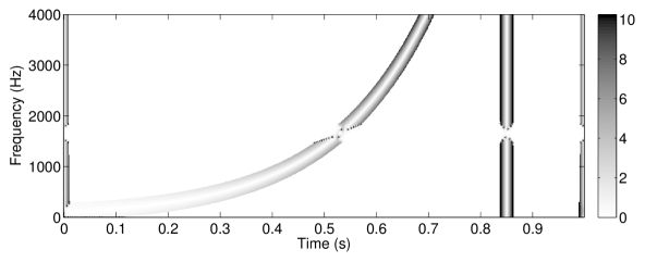
(Figure 1C)

III Full Phase Gradient Estimation And Integration

In this section, we present formulas for estimating partial derivatives of the STFT phase $\left(\Delta_{\text{f}}\phi_{\text{a}}\right)$ and $\left(\Delta_{\text{t}}\phi_{\text{a}}\right)$ and present an adaptive integration algorithm which takes them both into account to produce an adjusted synthesis phase $\phi_{\text{s}}$ to be used in (10).

The formulas exploit the well known phase unwrapping procedure which involves taking the principal argument of an angle. We adopt the notation from [22] and define the principal argument as

$$\left[x\right]_{2\pi}=x-2\pi\left\lceil\frac{x}{2\pi}\right\rfloor,$$ (12)

where $\lceil\cdot\rfloor$ denotes rounding towards the closest integer.

The well known phase differentiation in the time direction (involving conversion to heterodyned [5] phase difference and back) can be written as

$$\left(\Delta_{\text{t,back}}\phi_{\text{a}}\right)(m,n)=$$ (13)

$$\frac{1}{a_{\text{a}}}\left[\phi_{\text{a}}(m,n)-\phi_{\text{a}}(m,n-1)-\frac{2\pi ma_{\text{a}}}{M}\right]_{2\pi}+\frac{2\pi m}{M},$$

which is a modified backward difference scheme. The forward difference scheme can be written similarly

$$\left(\Delta_{\text{t,fwd}}\phi_{\text{a}}\right)(m,n)=$$ (14)

$$\frac{1}{a_{\text{a}}}\left[\phi_{\text{a}}(m,n+1)-\phi_{\text{a}}(m,n)-\frac{2\pi ma_{\text{a}}}{M}\right]_{2\pi}+\frac{2\pi m}{M}$$

and the centered difference is simply an average of the two

$$\left(\Delta_{\text{t,cent}}\phi_{\text{a}}\right)(m,n)=$$ (15)

$$\frac{1}{2}\left(\left(\Delta_{\text{t,back}}\phi_{\text{a}}\right)(m,n)+\left(\Delta_{\text{t,fwd}}\phi_{\text{a}}\right)(m,n)\right).$$

Any of the schemes can be used in place of $\Delta_{\text{t}}$. In our experience $\Delta_{\text{t,cent}}$ is the most suitable. Similarly, the differentiation in the frequency direction can be performed using the backward scheme

$$\left(\Delta_{\text{f,back}}\phi_{\text{a}}\right)(m,n)=\frac{1}{b_{\text{a}}}\left[\phi_{\text{a}}(m,n)-\phi_{\text{a}}(m-1,n)\right]_{2\pi},$$ (16)

the forward scheme

$$\left(\Delta_{\text{f,fwd}}\phi_{\text{a}}\right)(m,n)=\frac{1}{b_{\text{a}}}\left[\phi_{\text{a}}(m+1,n)-\phi_{\text{a}}(m,n)\right]_{2\pi},$$ (17)

or the centered scheme

$$\left(\Delta_{\text{f,cent}}\phi_{\text{a}}\right)(m,n)=$$ (18)

$$\frac{1}{2}\left(\left(\Delta_{\text{f,back}}\phi_{\text{a}}\right)(m,n)+\left(\Delta_{\text{f,fwd}}\phi_{\text{a}}\right)(m,n)\right).$$

Having the means for estimating the phase partial derivatives, the RTPGHI algorithm [19] can be invoked with few modifications. In its essence, the method proceeds by processing one frame at a time computing the synthesis phase of the current $n$-th frame $\phi_{\text{s}}(\cdot,n)$. It requires storing the already computed phase $\phi_{\text{s}}(\cdot,n-1)$ and the time derivative $\left(\Delta_{\text{t}}\phi_{\text{a}}\right)(\cdot,n-1)$ of the previous $(n-1)$-th frame and further, it requires access to the coefficients of the previous, current and one “future” frame ($c(\cdot,n-1)$, $c(\cdot,n)$ and $c(\cdot,n+1)$) assuming the centered differentiation scheme (15) is used for computing $\left(\Delta_{\text{t}}\phi_{\text{a}}\right)(\cdot,n)$. Before the algorithm starts $\left(\Delta_{\text{t}}\phi_{\text{a}}\right)(m,n)$ and $\left(\Delta_{\text{f}}\phi_{\text{a}}\right)(m,n)$ are computed for all $m$ and current $n$. The algorithm starts by selecting the frequency bin $m_{\text{h}}$ of the coefficient with the highest magnitude from the previous $(n-1)$-th frame and propagates the phase along the time direction to the current frame using $\eqref{eq:synphase2}$ such that $\phi_{\text{s}}(m_{\text{h}},n)$ is obtained. Up to this point, the procedure is equivalent with the classical PV. The way how the phase of the remaining coefficients is obtained is different since the phase can now be propagated also in the frequency direction from the already computed phase in the current frame. The phase propagation direction is decided on-the-fly according to the magnitude of the coefficients.

The steps of the algorithm are summarized in Alg. 1.

Input: Phase time derivative $\left(\Delta_{\text{t}}\phi_{\text{a}}\right)$ and magnitude $s$ of frames $n$ and $n-1$, phase frequency derivative $\left(\Delta_{\text{f}}\phi_{\text{a}}\right)$ for frame $n$, estimated phase $\phi_{\text{s}}$ for frame $n-1$ and relative tolerance $\mathit{tol}$.

Output: Phase estimate $\phi_{\text{s}}$ for frame $n$.

1 $\mathit{abstol}\leftarrow\mathit{tol}\cdot\max\left(s(m,n)\cup s(m,n-1)\right)$;

2 Create set $\mathcal{I}=\left\{m:s(m,n)>\mathit{abstol}\right\}$;

3 Assign random values to $\phi_{\text{s}}(m,n)$ for $m\notin\mathcal{I}$;

4 Construct a self-sorting max heap [23] for $(m,n)$ tuples;

5 Insert $(m,n-1)$ for $m\in\mathcal{I}$ into the heap;

6 while $\mathcal{I}$ is not $\emptyset$  do

7       $(m_{\text{h}},n_{\text{h}})\leftarrow$ remove the top of the heap;

8      

9      if $n_{\text{h}}=n-1$ then

10             if $(m_{\text{h}},n)\in\mathcal{I}$ then

11                   $\phi_{\text{s}}(m_{\text{h}},n)\leftarrow\phi_{\text{s}}(m_{\text{h}},n-1)+\frac{a_{\text{s}}}{2}\left(\left(\Delta_{\text{t}}\phi_{\text{a}}\right)(m_{\text{h}},n-1)+\left(\Delta_{\text{t}}\phi_{\text{a}}\right)(m_{\text{h}},n)\right)$;

12                   Remove $(m_{\text{h}},n)$ from $\mathcal{I}$;

13                   Insert $(m_{\text{h}},n)$ into the heap;

14                  

15             end if

16            

17       end if

18      if $n_{\text{h}}=n$ then

19             if $(m_{\text{h}}+1,n)\in\mathcal{I}$ then

20                   $\phi_{\text{s}}(m_{\text{h}}+1,n)\leftarrow\phi_{\text{s}}(m_{\text{h}},n)+\frac{b_{\text{s}}}{2}\left(\left(\Delta_{\text{f}}\phi_{\text{a}}\right)(m_{\text{h}},n)+\left(\Delta_{\text{f}}\phi_{\text{a}}\right)(m_{\text{h}}+1,n)\right)$;

21                   Remove $(m_{\text{h}}+1,n)$ from $\mathcal{I}$;

22                   Insert $(m_{\text{h}}+1,n)$ into the heap;

23                  

24             end if

25            if $(m_{\text{h}}-1,n)\in\mathcal{I}$ then

26                   $\phi_{\text{s}}(m_{\text{h}}-1,n)\leftarrow\phi_{\text{s}}(m_{\text{h}},n)-\frac{b_{\text{s}}}{2}\left(\left(\Delta_{\text{f}}\phi_{\text{a}}\right)(m_{\text{h}},n)+\left(\Delta_{\text{f}}\phi_{\text{a}}\right)(m_{\text{h}}-1,n)\right)$;

27                   Remove $(m_{\text{h}}-1,n)$ from $\mathcal{I}$;

28                   Insert $(m_{\text{h}}-1,n)$ into the heap;

29                  

30             end if

31            

32       end if

33      

34 end while

Algorithm 1 Phase Gradient Heap Integration for $n$-th frame

Note that the algorithm employs trapezoidal integration rule for the phase propagation on lines 1, 1 and 1. Line 1 implements (8), but the integration is also performed in the vertical (frequency) direction (lines 1, 1) employing the frequency phase derivative estimate $\left(\Delta_{\text{f}}\phi_{\text{a}}\right)$. The phase for each frequency bin is however computed only once. Which equation is used is decided adaptively according to the magnitude $s$ with the help of the max heap [23]. The max heap is a dynamic data structure that always places coordinates $(m,n)$ of the coefficient with the highest magnitude on top. It is populated by the coordinates of the coefficients with already known phase which are possible candidates from which the phase can be propagated further. At the beginning of the algorithm, all frequency bins from the previous frame with significant magnitude are inserted into the heap (line 5). In the first iteration, the only possible phase propagation direction is the time direction on line 1. The coordinates of the just computed coefficient are inserted into the heap (line 13). In the next iteration, two options are possible. Either the same procedure is repeated with another frequency bin from the previous frame, or the extracted top of the heap belongs to the current frame $n$. In that case, the phase is propagated in the frequency direction to both neighboring frequency bins on lines 1 and 1. Both neighbors are then inserted into the heap and in the next step, the integration continues with extracting the new heap top and spreading the phase further.

Fig. 1 shows examples of how the phase is spread for several signals. The orientation of the arrow identifies the line in the algorithm as follows: 1 ($\rightarrow$), 1 ($\uparrow$) and 1($\downarrow$).

Figure 1: Conceptual spectrograms overlaid with the phase spreading paths: a) pure sinusoid, b) linear chirp, c) two sinusoids, d) before impulse peak, e) after impulse peak. Coefficients with magnitude 1 are below the tolerance of the algorithm.

IV Evaluation

This section is devoted to the testing and evaluation of the proposed PV. We present the STFT setting used and summarize results of a listening test.

In the evaluation of the proposed PV we used a 4092 samples long Hann window, set the number of frequency channels to $M=8192$ and fixed the synthesis time step to $a_{\text{s}}=1024$, changing $a_{\text{a}}$ according to (5) rounded to the closest integer. All sound excerpts were sampled at 44.1 kHz. The tolerance in Algorithm 1 was set to $\mathit{tol}=10^{-6}$. We compared the results with the following algorithms and software:

• Classical PV (PV) using the same setting as the proposed algorithm.

• élastique PRO (EL) [24] (accessed through the Sonic API http://www.sonicapi.com with the help of a script from the TSM toolbox [25]).

• IRCAM Lab TS 1.0.11 (IR) [26] (demo version) with the quality set to high, polyphonic setting and enabled transient preservation.

• melodyne4 4.1.0 (ME) [27] (trial version) with the universal algorithm.

It is worth mentioning that both IR and ME offer additional modes specialized to specific types of audio signals (voice, percussions, etc.). We have intentionally used the most universal options.

The listening tests were performed for $\alpha=\left\{1.5,2\right\}$ using a web interface [28]. In the tests, we used the proposed algorithm as the reference and asked subjects to rate presented sound examples on the relative comparison category rating (CCR) scale [29] (3 Much better, 2 Better, 1 Slightly better, 0 About the same, $-1$ Slightly worse, $-2$ Worse, $-3$ Much worse). Each time, 5 sound examples were rated; 4 for the algorithms and software mentioned above and 1 was a hidden reference in the fashion of the MUSHRA test [30] (similar tests were performed in [22]). A total number of 8 subjects with background in acoustics participated in the test. Two subjects were removed from the evaluation because they regularly failed to identify the hidden reference. Table I is a list of excerpts used and Table II shows the average CCR for the individual sound excerpts. As expected, the classical PV (PV) was consistently rated worse than the proposed method.

For $\alpha=1.5$, EL and IR were rated close to the proposed method, with the exception of Latino and DrumSolo for EL which were slightly worse mainly due to poorer transient preservation. ME was rated slightly worse consistently.

For $\alpha=2$, both EL and ME were rated worse than the proposed method consistently. For IR, complex mixes PeterGabriel and EddieRabbit were rated slightly better than the proposed algorithm. We suspect that this is mainly due to the active transient preservation in IR, which results in a shorter attack time of the transients. On the other hand, the female voice in Musetta is slightly more “phasy” than the proposed method, which could be a reason for why it was rated slightly worse.

All sound examples are available at http://ltfat.github.io/notes/050.

Table I: List of sound examples

Name	Description
CastViolin	Solo violin overlaid with castanets from [25].
DrumSolo	A solo on a drum set from [25].
Latino	Pan flute, guitar and percussion.
Musetta	An excerpt from a song Ophelia’s song performed by Musetta from the Nice to meet you! album (female solo singing).
March	An excerpt from Radetzky March by Johann Strauss performed by an orchestra.
PeterGabriel	An excerpt from a song Sledgehammer performed by Peter Gabriel from the album So.
EddieRabbit	An excerpt from a song Early in the morning performed by Eddie Rabbit from the album Step by Step.

Table II: Comparison mean opinion score for sound examples

	$\alpha=2$				$\alpha=1.5$
	PV	EL	ME	IR	PV	EL	ME	IR
CastViolin	$-2.7$	$-0.4$	$-0.8$	$-0.3$	$-2.3$	$0.3$	$-1.0$	$-0.3$
DrumSolo	$-2.9$	$-2.0$	$-2.7$	$0.5$	$-2.8$	$-0.8$	$-0.6$	$0.0$
Latino	$-1.4$	$-1.3$	$-0.3$	$0.3$	$-1.7$	$-0.9$	$-1.5$	$-0.5$
Musetta	$-1.6$	$-1.0$	$-2.1$	$-0.8$	$-2.1$	$0.2$	$-0.8$	$0.1$
March	$-1.3$	$-1.8$	$-1.1$	$-0.7$	$-1.3$	$-0.6$	$-0.7$	$-0.3$
PeterGabriel	$-1.1$	$-1.8$	$-1.2$	$0.9$	$-2.0$	$-0.5$	$-1.1$	$-0.2$
EddieRabbit	$-0.7$	$-2.0$	$-1.4$	$1.3$	$-2.2$	$-0.2$	$-0.8$	$0.1$
Avg.	$-1.7$	$-1.5$	$-1.4$	$0.2$	$-2.1$	$-0.3$	$-0.9$	$-0.2$

V Conclusion

We presented a novel method for adjusting phase in PV used for time-scaling of audio signals. The method is simple in the sense that it works automatically and it does not require analyzing the signal content. The listening test shows that it is competitive with state-of-the-art time-stretching in commercial software solutions.

While the proposed method does preserve transients without the necessity of detecting them, it also stretches them together with the rest of the signal. If true transient preservation, or rather transient sharpening is desired, their detection and special treatment seems to be unavoidable. The transient processing method by Röbel [10] is a suitable candidate for such task as it uses already computed $\left(\Delta_{\text{f}}\phi_{\text{a}}\right)$ for transient detection.

Unfortunately, the current implementation of the proposed method is not optimal for voiced monophonic speech signals. We expect that this is due to the possible phase shift between the fundamental and the partials. Specialized PV variants (e.g. Moinet and Dutoid [16]) provide perceptually better results. Therefore, in the future, we plan to enhance the proposed PV with the shape-preserving property. Moreover, an extension of PGHI to more general filter banks has been proposed in [31]. The design of a phase vocoder employing a filter bank with variable time-frequency resolution could provide an interesting starting point for further developments.

References

- [1] J. L. Flanagan and R. M. Golden, “Phase vocoder,” Bell System Technical Journal, vol. 45, no. 9, pp. 1493–1509, 1966.
- [2] M. R. Portnoff, “Time-scale modification of speech based on short-time Fourier analysis,” Ph.D. dissertation, Massachusetts Institute of Technology, 1978.
- [3] E. Moulines and J. Laroche, “Non-parametric techniques for pitch-scale and time-scale modification of speech,” Speech Communication, vol. 16, no. 2, pp. 175 – 205, 1995.
- [4] J. Laroche and M. Dolson, “Phase-vocoder: About this phasiness business,” in IEEE ASSP Workshop on Applications of Signal Processing to Audio and Acoustics, Oct 1997, p. 4.
- [5] ——, “Improved phase vocoder time-scale modification of audio,” IEEE Transactions on Speech and Audio Processing, vol. 7, no. 3, pp. 323–332, May 1999.
- [6] U. Zölzer, Ed., DAFX: Digital Audio Effects. New York, NY, USA: John Wiley & Sons, Inc., 2002.
- [7] M. Liuni and A. Röbel, “Phase vocoder and beyond,” Musica/Tecnologia, vol. 7, no. 0, 2013.
- [8] J. Driedger and M. Müller, “A review of time-scale modification of music signals,” Applied Sciences, vol. 6, no. 2, 2016.
- [9] C. Duxbury, M. Davies, and M. B. Sandler, “Improved time-scaling of musical audio using phase locking at transients,” in Audio Engineering Society Convention 112, Apr 2002.
- [10] A. Röbel, “A new approach to transient processing in the phase vocoder,” in Proc. Int. Conf. Digital Audio Effects (DAFx–03), Sep 2003.
- [11] E. Ravelli, M. Sandler, and J. P. Bello, “Fast implementation for non-linear time-scaling of stereo signals,” in Proc. Int. Conf. Digital Audio Effects (DAFx–05), Sep 2005.
- [12] F. Nagel and A. Walther, “A novel transient handling scheme for time stretching algorithms,” in Audio Engineering Society Convention 127, Oct 2009.
- [13] J. Driedger, M. Müller, and S. Ewert, “Improving time-scale modification of music signals using harmonic-percussive separation,” IEEE Signal Processing Letters, vol. 21, no. 1, pp. 105–109, Jan 2014.
- [14] E. S. Ottosen and M. Dörfler, “A phase vocoder based on nonstationary Gabor frames,” CoRR, vol. abs/1612.05156, 2016. [Online]. Available: http://arxiv.org/abs/1612.05156
- [15] A. Röbel, “A shape-invariant phase vocoder for speech transformation,” in Proc. Int. Conf. Digital Audio Effects (DAFx–10), Graz, Austria, Sep. 2010, pp. 1–1.
- [16] A. Moinet and T. Dutoit, “PVSOLA: A phase vocoder with synchronized overlap-add,” in Proc. Int. Conf. Digital Audio Effects (DAFx–11), Sep 2011.
- [17] T. F. Quatieri and R. J. McAulay, “Shape invariant time-scale and pitch modification of speech,” IEEE Transactions on Signal Processing, vol. 40, no. 3, pp. 497–510, March 1992.
- [18] D. Griffin and J. Lim, “Signal estimation from modified short-time Fourier transform,” IEEE Transactions on Acoustics, Speech and Signal Processing, vol. 32, no. 2, pp. 236–243, Apr 1984.
- [19] Z. Průša and P. L. Søndergaard, “Real-time spectrogram inversion using phase gradient heap integration,” in Proc. Int. Conf. Digital Audio Effects (DAFx–16), Sep 2016, pp. 17–21.
- [20] Z. Průša and P. Rajmic, “Toward high-quality real-time signal reconstruction from STFT magnitude,” IEEE Signal Processing Letters, vol. 24, no. 6, June 2017.
- [21] Z. Průša, P. Balazs, and P. L. Søndergaard, “A Noniterative Method for Reconstruction of Phase from STFT Magnitude,” IEEE/ACM Trans. on Audio, Speech, and Lang. Process., vol. 25, no. 5, May 2017.
- [22] S. Kraft, M. Holters, A. von dem Knesebeck, and U. Zölzer, “Improved PVSOLA time-stretching and pitch-shifting for polyphonic audio,” in Proc. Int. Conf. Digital Audio Effects (DAFx–12), Sep 2012.
- [23] J. W. J. Williams, “Algorithm 232: Heapsort,” Communications of the ACM, vol. 7, no. 6, pp. 347–348, 1964.
- [24] zplane.development GmbH & Co. KG, “élastique time stretching & pitch shifting SDKs,” web resource: http://licensing.zplane.de/technology\#elastique.
- [25] J. Driedger and M. Müller, “TSM toolbox: MATLAB implementations of time-scale modification algorithms,” in Proc. Int. Conf. Digital Audio Effects (DAFx–14), Sep 2014.
- [26] IRCAM Analysis Synthesis Team, “IrcamLab Transpose/Stretching application v1.0.11,” web resource: http://www.ircamlab.com/products/p1680-TS.
- [27] Celemony Software GmbH, “melodyne4 studio: Melodyne player 4.1.0,” web resource: http://www.celemony.com/en/melodyne/what-is-melodyne.
- [28] N. Jillings, D. Moffat, B. De Man, and J. D. Reiss, “Web Audio Evaluation Tool: A browser-based listening test environment,” in 12th Sound and Music Computing Conference, July 2015.
- [29] ITU-T Recommendation P.800, “Methods for subjective determination of transmission quality,” International Telecommunication Union, Geneva, Switzerland, 1996.
- [30] ITU-T Recommendation BS.1534-3, “Method for the subjective assessment of intermediate quality level of coding systems,” International Telecommunication Union, Geneva, Switzerland, 2015.
- [31] Z. Průša and N. Holighaus, “Non-iterative filter bank phase (re)construction,” in Proc. 25th European Signal Processing Conference (EUSIPCO–2017), Aug 2017.