Realistic Counterfactual Explanations by Learned Relations

Abstract

Many existing methods of counterfactual explanations ignore the intrinsic relationships between data attributes and thus fail to generate realistic counterfactuals. Moreover, the existing models that account for relationships require domain knowledge, which limits their applicability in complex real-world applications. In this paper, we propose a novel approach to realistic counterfactual explanations that preserve the relationships and minimise experts’ interventions. The model directly learns the relationships by a variational auto-encoder with minimal domain knowledge and then learns to perturb the latent space accordingly. We conduct extensive experiments on both synthetic and real-world datasets. The experimental results demonstrate that the proposed model learns relationships from the data and preserves these relationships in generated counterfactuals. In particular, it outperforms other methods in terms of Mahalanobis distance, and the constraint feasibility score.

Keywords Explainable machine learning, realistic counterfactual explanations

1 Introduction

In light of widespread of deep learning models in numerous engineering and medical applications, being able to explain these models has become an important issueŠtrumbelj and Kononenko (2014); Datta et al. (2016). There are two directions that focus on providing explanations to the models and consequent decisions made by them. The first group focuses on explanations by means of local classification boundaries (e.g. LIME Ribeiro et al. (2016)) to explain why a give sample was classified this way, the other one focuses on an entire model and present importance of each feature (e.g. SHAP Lundberg and Lee (2017)). Both approaches assign each predictor an importance weight to a particular prediction. For example, if a bank loan was rejected, then the bank can employ the SHAP values to explain the reasons behind this decision i.e. to let the client know that his/her salary was an important factor in declining the loan. Although these approaches are useful in helping to uncover mysterious machine learning models that are often treated as black boxes, there are a number of applications where information about feature importance is not sufficient and counterfactual explanations are more favorable. Going back to the example of credit predication: a client whose loan application is rejected, would like to know how can he/she improve the chances in getting the application approved next time, rather than just being presented with the importance of each factor. In other words, rather than just explaining what factors played a role in rejecting the loan, provide a recommendation on what exactly needs to be done to reach a positive decision next time. The method of counterfactual explanations focuses on answering the question - How could I get the desired target, given that I am in the current situation with respect to the employed decision model?

In a recent review on methods for counterfactual explanations Verma et al. (2020), the nearest counterfactual explanation was identified as one of the most popular methods in generating counterfactuals. The method provides a nearest explanation with a desired output Wachter et al. (2018) by optimising the following criterion

$$\mathop{\arg\text{min}}\limits_{\mathbf{x}^{CF}}\ \lambda(f(\mathbf{x}^{CF})-y^{CF})^{2}+d(\mathbf{x},\mathbf{x}^{CF}),$$ (1)

where $\mathbf{x}$ is a sample, $\mathbf{x}^{CF}$ is a corresponding generated counterfactual, $y^{CF}$ is the target label for counterfactual and $\lambda$ is a scale factor that controls a trade-off of accuracy and closeness. Some other constraints such as sparsity and feasibility can be added to generate more favorable explanations Dandl et al. (2020); Karimi et al. (2020). However, recent research raises concerns about feasibility in counterfactual explanations Mahajan et al. (2019) in real-world applications. For example, in a medical application where we are giving suggestions to patients, we should consider that the blood pressure and blood mass index (BMI) are positively correlated. Therefore, we should not suggest decreasing blood pressure while increasing BMI. Indeed, some methods Karimi et al. (2020, 2020); Downs et al. (2020) have been proposed to address this very problem, however there are some downsides.

Existing models and their drawbacks Existing methods all assume complete or at least partial domain knowledge, which is not always can be put into practice as part of real-world applications. Mahajan et al. proposed to modify the optimisation criterion in such a way that expert knowledge (i.e. prior examples or external oracle) is taken into account and the model is retrained accordinglyMahajan et al. (2019). Downs et al. proposed to use conditional subspace variational auto-encoder that generates multiple recourse satisfying underlying structure of the data with end-user specified constraints Downs et al. (2020). Karimi et al. Karimi et al. (2020, 2020) assumed that at least partial causal graph is available during training. While these approaches indeed improves the quality of generated counterfactuals, these methods requires domain knowledge which is often hard to obtain, especially in areas such as biology or medicine that frequently deal with high-dimensional feature spaces. Practically, only labeled data is available without or with minimal expert input. This practical limitation motivates us to search for methods of causal inference Pearl et al. (2016) in order to infer the inner relationships between observed variables.

In this paper, we propose a counterfactual explanation method that assumes no prior knowledge on relationships between the variables in an application domain. To learn the relationships between data attributes, our method first trains a variational auto-encoder (VAE) that is based on DAG-GNN Yu et al. (2019). Then, the proposed method learns a modulation network that takes the query data points and corresponding target labels as inputs, and perturb the latent representations of the data points so that counterfactuals can be constructed by the perturbed latent representations. To make sure that the generated counterfactuals preserve the learned relationships, we use adversarial training to match the counterfactual latent distribution to the query data latent distribution. The proposed approach thus can provide a realistic and satisfactory recommendation by generating counterfactuals without any prior domain knowledge.

The main contributions of this work are as follows:

• We propose a novel model that considers relationships between attributes and gives realistic counterfactual explanations of machine learning model.

• The model does not need any prior domain knowledge on predictors’ correlation and is thus more flexible and useful in complex real-world settings where prior knowledge is difficult to obtain.

• The extensive experiments on both synthetic and real-world datasets demonstrate the feasibility of the proposed model.

2 Background and Related Work

Causal relationships. Causal relationships are commonly represented by directed acyclic graphs (DAG): $\mathcal{G}=(\mathcal{V},\mathcal{E})$, with $\mathcal{V}$ being a set of nodes representing attributes $\{v_{1},...,v_{L}\}$, and $\mathcal{E}$ denoting the directed edges corresponding to causal relations. The causal relations between variables can be modelled by a structural causal model (SCM) Peters et al. (2017):

$$v_{j}=f_{j}(\mathcal{P}_{j},\epsilon_{j})\ \ \ \ j=1,...,L,$$ (2)

where $\mathcal{P}_{j}$ denotes parents of $v_{j}$ (the nodes that point to node $v_{j}$) and $\epsilon_{j}$ is its corresponding exogenous variable. The problem has been extensively studied over the past decades Spirtes et al. (2000); Mooij et al. (2016); Glymour et al. (2019); Zhu et al. (2020). In this paper, our proposed method builds on an extension of VAE and implements DAG-GNN in accordance to Yu et al. (2019). The method learns a DAG from data which represents the relationships between data attributes. Note that here we consider undirected relationships, as in real-world applications it is impossible to intervene a variable independently of its causes and hence to infer a direct relationship. Mahajan et al. (2019).

Variational auto-encoder. VAE proposed by Kingma and Welling (2014) is a Bayesian neural network that learns to represent an observation $\mathbf{x}$ as a latent variable $\mathbf{z}$. The model aims at maximizing the likelihood $\texttt{log}\ p(\mathbf{x})$. While the actual posterior $p(\mathbf{x}|\mathbf{z})$ is intractable, VAE uses variational posterior $q(\mathbf{z}|\mathbf{x})$ to approximate it. The training objective can be constructed by the Evidence Lower Bound (ELBO):

$$\mathcal{L}(\theta,\phi;\mathbf{x},\mathbf{z})=\mathbb{E}_{q_{\phi}(\mathbf{x}|\mathbf{z})}\big{[}\log p_{\theta}(\mathbf{x}|\mathbf{z})\big{]}-\texttt{D}_{KL}\big{(}q_{\phi}(\mathbf{z}|\mathbf{x})||p(\mathbf{z})\big{)}$$ (3)

where $\theta$ and $\phi$ are neural network parameters. In this paper, we build a generative model based on VAE, specifically built on DAG-GNN Yu et al. (2019) then generate counterfactuals through the decoder by disturbing the latent representations.

Figure 1: A flowchart model. Stage 1: the encoder and decoder are trained to reconstruct samples. Stage 2: a modulation network is trained to generate disturbance on the latent representation, that is used to construct counterfactuals by the decoder.

Counterfactual explanation in machine learning. Counterfactual explanation in machine learning has received increasing attention in research, especially for high-impact areas such as financial or healthcare Verma et al. (2020). A number of methods have been proposed to give an optimal solution to the problem of generating counterfactuals Albini et al. (2020); Kommiya Mothilal et al. (2021); Parmentier and Vidal (2021). Wachter et al. (2018) proposes to generate counterfactuals to explain models by solving the optimization problem formulated by Equation 1. Several extensions Dandl et al. (2020); Mothilal et al. (2020); Grath et al. (2018) have been proposed based on this criterion. Concerns about feasibility, actionability and sparsity in counterfactual explanations have been raised Mahajan et al. (2019); Karimi et al. (2020); Keane and Smyth (2020). A counterfactual explanation is said to be feasible when it captures the relationships between attributes. Actionability aims at providing practical counterfactual and depends on the affordability of individuals on implementing the counterfactual Ferrario and Loi (2020). For example, increasing the age for 20 years is expensive and meaningless for a person in real world. Sparsity applies when shorter explanations are more comprehensible to humans Verma et al. (2020), where ideally, the counterfactual changes only a small number of attributes. In this paper, we focus on generating feasible counterfactual. A similar task was investigated by Albini et al. (2020), that generated counterfactual explanations for a range of Bayesian network classifiers. While the method does focus on explanations built from relations of influence between variables, it is specifically designed for Bayesian network. On contrary, our method, in theory, can be used for any classifier that allows gradient back propagation. Another method proposed by Mahajan et al. (2019) requires expert knowledge. Instead our method can automatically learn the intrinsic relationships between attributes and unlike Karimi et al. (2020, 2020); Downs et al. (2020), the proposed method does not rely on prior knowledge.

3 The model description

The major issue of generating feasible counterfactuals consists in determining the intrinsic relationships in the data. As stated earlier, existing methods Mahajan et al. (2019); Karimi et al. (2020, 2020); Downs et al. (2020) have assumed full or at least some knowledge about the relationships, evidently this assumption is not always practical. Potentially, methods of causal inference, such as Mooij et al. (2016); Zhu et al. (2020) could be used to determine the causal relationships first and then generate valid counterfactuals by subsequent models of counterfactuals generation. However, such approach requires several models which might result in additional computational costs, especially when methods of exact Bayesian structure discovery are used to learn the structureKoivisto and Sood (2005). The latter are known to be computationally expensive. Therefore, an end-to-end model that directly learns the relationships and generates counterfactuals is preferred.

Figure 1 presents an flowchart of the proposed end-to-end model. To learn the relationships, we employ DAG-GNN Yu et al. (2019) which is designed to learn the directed relationships between the data attributes. This model captures intrinsic relationships between the attributes i.e. the DAG with attributes as nodes. The adjacency matrix helps the model preserve the relationships and the VAE architecture makes it possible to generate valid counterfactuals. One may argue that conditional VAE Sohn et al. (2015) can also provide in-distribution counterfactuals. However, the in-distribution counterfactuals do not directly imply valid relationships between the attributes. Figure 2 demonstrates an example, where the yellow counterfactual is in-distribution but not a favorable counterfactual. The DAG-GNN is firstly trained to learn the relationships between the attributes and to reconstruct the samples correctly. Then the counterfactuals are generated by perturbing the learned latent space. To match the perturbed latent distribution to the true latent distribution, we borrow the adversarial idea from adversarial auto-encoder (AAE) Makhzani et al. (2015) and use adversarial training. In the following sections, a rough introduction of DAG-GNN Yu et al. (2019) is given. Then, the details on how the samples are perturbed in the latent space are provided.

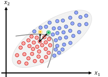
Figure 2: The red and blue circles are data instances with two attributes positively related. The yellow and green circles are generated counterfactual.

3.1 Stage 1: Base VAE Pretrain

VAE serves as the core model for generating counterfactuals. We first pretrain VAE that reconstructs a given sample accurately. We follow the construction process of DAG-GNN Yu et al. (2019). In this section, we provide only a brief descriptions of DAG-GNN, for more details, please refer to Yu et al. (2019).

Typically, a sample $\mathbf{x}$ is a vector where every attribute is a scalar. The representation can be generalized to $m$ dimensions per attribute. Denote $\mathbf{V}\in\mathbb{R}^{L\times m}$ to represent a sample with $L$ attributes and each attribute has $m$ dimensions. DAG-GNN considers the relationships between attributes by a structural equation model (SEM) of the following form:

$$\mathbf{V}=\mathbf{A}^{T}\mathbf{V}+\mathbf{Z},$$ (4)

where $\mathbf{A}\in\mathbb{R}^{L\times L}$ denotes the adjacency matrix of directed relationships between the nodes and $\mathbf{Z}\in\mathbb{R}^{L\times m}$ denotes the exogenous variables. Then, the equation can be represented as $\mathbf{V}=(\mathbf{I}-\mathbf{A}^{T})^{-1}\mathbf{Z}$. The decoder’s architecture can then be designed in a more general form by taking non-linear transformations:

$$\mathbf{V}=f^{caus}_{2}\big{(}(\mathbf{I}-\mathbf{A}^{T})^{-1}f^{caus}_{1}(\mathbf{Z})\big{)},$$ (5)

where $f^{caus}_{1}$ and $f^{caus}_{2}$ are two parameterized functions that we choose to represent by a multilayer perceptron (MLP). Similarly, the encoder is constructed as:

$$\mathbf{Z}=f^{caus}_{4}\big{(}(\mathbf{I}-\mathbf{A}^{T})f^{caus}_{3}(\mathbf{V})\big{)},$$ (6)

where $f^{caus}_{3}$ and $f^{caus}_{4}$ can be considered as inverses of $f^{caus}_{2}$ and $f^{caus}_{1}$. Note that as we perform non-linear transformations and $\mathbf{Z}$ is treated as latent variables, the choice of hidden dimension $d$ of $\mathbf{Z}$ is arbitrary and so $\mathbf{Z}\in\mathbb{R}^{L\times d}$. Following the VAE construction procedure, the evidence lower bound (ELBO) is given by:

$$\mathcal{L}_{ELBO}=-\texttt{KL}(q(\mathbf{Z}|\mathbf{V})||p(\mathbf{Z}))+E_{q(\mathbf{Z}|\mathbf{V})}\big{[}\log p(\mathbf{V}|\mathbf{Z})\big{]}$$ (7)

Specifically, the method takes $f^{caus}_{1}$ as identity mapping, $f^{caus}_{2}$ as an MLP, and $f^{caus}_{3}$, $f^{caus}_{4}$ as an MLP and identity mapping, respectively. For simplicity, the prior is assumed to be the standard normal distribution. In addition to the ELBO loss, an acyclity constraint is added to make $\mathbf{A}$ acyclic:

$$\texttt{tr}\big{[}(\mathbf{I}+\alpha\mathbf{A}\circ\mathbf{A})^{L}\big{]}-L=0$$ (8)

As a result of training by the combined loss listed above, we obtain a VAE that is capable of reconstructing the given samples as well as detecting the relationships between the data attributes.

3.2 Stage 2: Latent Space Disturbance

To avoid notation cluttering, in this subsection, we assume all attributes are scalars and denote $\mathbf{z}\in\mathbb{R}^{d}$ as the latent representation of a sample $\mathbf{x}\in\mathbb{R}^{L}$. Our objective here is to train an effective modulation network denoted by $f^{mod}(\cdot)$ that can perturb the latent representation in a desirable way. Both, a sample $\mathbf{x}$ and a target label $y^{CF}$ are passed to the model. The modulation function $f^{mod}$ that computes the latent code perturbation $\boldsymbol{\delta}$, takes a concatenated vector of $\mathbf{x}$ and $y^{CF}$:

$$\boldsymbol{\delta}=f^{mod}(\mathbf{x}||y^{CF}),$$ (9)

where $||$ denotes concatenation. Given a sample $\mathbf{x}$, its latent representation $\mathbf{z}$ is obtained by eq. 6, and the perturbation is added to its latent representation to obtain the latent representation of a corresponding counterfactual $\mathbf{z}^{CF}=\mathbf{z}+\boldsymbol{\delta}$, then the corresponding counterfactual is produced by decoding $\mathbf{z}^{CF}$. Formally, the procedure of generating counterfactual $\mathbf{x}^{CF}$ is given by:

$$\mathbf{x}^{CF}=f^{caus}_{2}\big{(}(\mathbf{I}-\mathbf{A}^{T})^{-1}f^{caus}_{1}(\mathbf{z}^{CF})\big{)}.$$ (10)

Empirically, we observed that a large disturbance $\boldsymbol{\delta}$ at the very beginning of the training made the training unstable. Therefore, to mitigate this effect, the disturbance vector $\boldsymbol{\delta}$ is scaled by a factor $\gamma$ (set to $0.05$).

Objectives functions. Recall that we impose the requirement for the counterfactual to be valid i.e. to have a predefined target label. Following Mahajan et al. (2019), we introduce a classification loss over the generated counterfactuals as follows:

$$\mathcal{L}_{class}=\sum^{N}_{i=1}\text{HingeLoss}(h(\mathbf{x}_{i}^{CF}),y_{i}^{CF},\beta),$$ (11)

where $h(\cdot)$ is black box model, and the hinge loss is defined over the probability $s_{y}$ as

$$\text{HingeLoss}(h(\mathbf{x}^{CF}),y^{CF},\beta)=\texttt{max}\{\texttt{max}_{y\neq y^{CF}}\{s_{y}(\mathbf{x}^{CF})\}-s_{y^{CF}}(\mathbf{x}^{CF}),-\beta\},$$ (12)

with $\beta$ being a pre-defined margin. This loss function ensures the score of our target label to be higher than any other label at least by $\beta$. Our second objective is to let the counterfactual to be as close to the original sample as possible. Furthermore, since we aim at minimizing the perturbation of the latent code that generates a counterfactual, we penalize large $\boldsymbol{\delta}$ in terms of its $L_{2}$ norm. Then, the nearest loss is defined as:

$$\mathcal{L}_{near}=\sum^{N}_{i=1}\big{(}\texttt{dist}(\mathbf{x}_{i},\mathbf{x}_{i}^{CF})+||\boldsymbol{\delta}_{i}||^{2}_{2}\big{)},$$ (13)

where $\texttt{dist}(\cdot)$ is a distance function which could be defined by $L_{1}$ or $L_{2}$ distances. Since the trained decoder can only decode from a specific distribution (i.e. the latent distribution of the training samples), we propose to match the distribution of $\mathbf{z}^{CF}$ to $\mathbf{z}$ in an adversarial training way. We train a discriminator $f^{dis}(\cdot)$ to classify $\mathbf{z}^{CF}$ and $\mathbf{z}$. The objective of $f^{mod}(\cdot)$ is to fool the discriminator by minimizing the loss function:

$$\mathcal{L}_{adv}=\sum^{N}_{i=1}-\texttt{log}(f^{dis}(\mathbf{z}_{i}^{CF})).$$ (14)

Conversely, the objective of the discriminator is to minimize the loss $\sum^{N}_{i=1}-(\texttt{log}(f^{dis}(\mathbf{z}_{i}))+\texttt{log}(1-f^{dis}(\mathbf{z}_{i}^{CF}))$. During the training stage, we iteratively optimize the modulation network $f^{mod}(\cdot)$ and the discriminator $f^{dis}(\cdot)$. This is similar to the training procedure of AAE Makhzani et al. (2015). While AAE matches the latent space to an assumed distribution (e.g. standard Gaussian distribution), we match the latent distribution of counterfactuals to the latent distribution of the training samples.

The above three optimisation criteria: the classification loss, the nearest loss and the adversarial loss, can be combined into the final objective function:

$$\mathcal{L}_{total}=\sum^{N}_{i=1}\Big{(}\alpha_{1}\text{HingeLoss}(h(\mathbf{x}_{i}^{CF}),y_{i}^{CF},\beta)+\alpha_{2}\big{(}\text{dist}(\mathbf{x}_{i},\mathbf{x}_{i}^{CF})+||\boldsymbol{\delta}_{i}||^{2}_{2}\big{)}+\alpha_{3}\big{(}-\log\ (f^{dis}(\mathbf{z}_{i}^{CF}))\big{)}\Big{)}$$ (15)

where $\alpha_{1},\alpha_{2},\alpha_{3}$ are hyperparameters to balance the effects of the three criteria.

4 Experiments

We conduct our method on both synthetic and real-world datasets to answer the following research questions:

• RQ1: How effective is our method in preserving the relationships when generating counterfactuals?

• RQ2: How can our method provide suggestions in a real-world machine learning application?

4.1 Experiment Settings

Datasets. We evaluate our approach on two synthetic datasets including a toy dataset and a complex nonlinear dataset, a publicly-available real-world simulated Bayesian network dataset Sangiovese and a real-world diabetes dataset Pima-Indians-Diabetes. The statistics of the datasets are shown in Table 1.

Table 1: Statistics of datasets. Splits mean the splits of train/val/test.

Datasets	Synthetic-toy	Synthetic-nonlinear	Sangiovese	Diabetes
# Classes	2	2	2	2
# Samples	20000	20000	11570	336
Train/val/test Splits	8:1:1	8:1:1	8:1:1	Leave-out-one

Compared methods. We implement the example-based Plain-CF method that was proposed in Wachter et al. (2018) with Hinge loss and $L_{2}$ norm. Following Dandl et al. (2020), we further implement another version of Plain-CF_K that adds an extra constraint on the distances to $k$-nearest neighbours. We also compare our method to the CF-VAE proposed in Mahajan et al. (2019). This is a base model that does not consider possible relationships between the predictors. To be consistent with the experimental setting in Mahajan et al. (2019) which manually label 10% of the counterfactuals, we compare the example-based VAE (EB-VAE) by manually labeling 10% of the counterfactuals and retrain the CF-VAE.

Evaluation metrics. The proposed approach is evaluated both quantitatively and qualitatively. For the quantitative metrics, we :

• Validity that is defined as a percentage of counterfactuals that are generated with correct labels.

• Constraint Feasibility Score $S$ that is the percentage of counterfactuals that preserve the relationships Mahajan et al. (2019); Downs et al. (2020). For example, the constraint feasibility score is 90% if 90% of the counterfactuals have two positively related attributes both increase or both decrease. For two relationships, the score is calculated as $2\frac{S_{1}S_{2}}{S_{1}+S_{2}}$ where $S_{1}$ and $S_{2}$ are the scores for the two relationships separately.

• Euclidean Distance measures the distance between counterfactuals and corresponding original samples. The distance is normalized by the diameter of the set of original samples. This metric measures how much the original sample should be perturbed to obtain a corresponding counterfactual.

• Mahalanobis Distance is another metric that accounts for covariance in the data. The distance between two points is defined as $D(\mathbf{x_{1}},\mathbf{x_{2}})=\sqrt{(\mathbf{x_{1}}-\mathbf{x_{2}})^{\top}\Sigma^{-1}(\mathbf{x_{1}}-\mathbf{x_{2}})}$ where $\Sigma$ denotes the covariance matrix.

It is worth noting that the distances as evaluation metrics might not accurately reflect the quality of generated counterfactuals. There are cases when in order to preserve the relationships between the attributes, a larger perturbation is required and hence results in larger distances. Figure 2 demonstrates an example of a dataset with attributes that exhibit a linear relationship, a generated counterfactual marked in yellow is closer in terms of Euclidean distance than the one marked in green, however such counterfactual does not account for linear relationship between the attributes, while the green counterfactual preserves the relationship. The Mahalanobis distance on the other hand would produce a smaller distance for the green counterfactual as it accounts for the data covariance.

The qualitative evaluations include visualization of selected pairs of attributes and their corresponding counterfactuals, as well as, $t$-SNE visualization of the complete attribute space. To visually verify that the relationships are preserved, we plot arrows connecting original samples with their corresponding counterfactuals.

Details on implementation. The models employed as black-box classifiers are two-layer MLPs with ReLU activation functions. We set the dimensions of the hidden layer to 32 for synthetic datasets and 16 for the Sangiovese dataset. The test accuracy of the two synthetic datasets, were nearly 98%, while for Sangiovese it was around 83%. We used the official Pytorch implementation of DAG-GNN, both the encoder and the decoder are two layers MLP with hidden size of 16 neurons, and the latent size of 4 neurons (we did not tune these two hyperparameters). Both the modulation network and the discriminator are two-layer MLPs with equal numbers of hidden units. For synthetic datasets, the modulation network was trained for 100 epochs while for Sangiovese, it was trained for 80 epochs. Grid search was used to tune the hyperparameters of the two networks where the hidden sizes were chosen from $[\texttt{32, 64}]$, the learning rates were chosen from $[\texttt{5e-4, 1e-3, 2e-3}]$ and the batch sizes were chosen from $[\texttt{16, 32}]$. The choice of hyperparameters did not significantly affect the validity that reached nearly $100\%$, and hence we chose the hyperparameters to maximise constraint feasibility score. The hyperparameters $\alpha_{1}$, $\alpha_{2}$ and $\alpha_{3}$ were set to $0.5$, $1$, and $0.5$, respectively. The codes are available at https://github.com/xintao-xiang/Realistic_CF/tree/multi_label.

4.2 Performances Comparison (RQ1)

Synthetic 5-variable Toy Dataset. The purpose of this experiment is to evaluate the proposed model on a toy dataset with linear relationships between the attributes. The data is generated using the following structural equations and noise distributions:

$$X_{1} =U_{1} \quad\quad\quad\quad U_{1} \sim\mathcal{N}(0,0.5)$$ (16)

$$X_{2} =U_{2} U_{2} \sim\mathcal{N}(0,0.5)$$ (17)

$$X_{3} =2X_{1}-X_{2}+U_{3} U_{3} \sim\mathcal{N}(0,0.5)$$ (18)

$$X_{4} =-2X_{3}+U_{4} U_{4} \sim\mathcal{N}(0,0.5)$$ (19)

$$X_{5} =\texttt{sin}(X_{3})+U_{5} U_{5} \sim\mathcal{N}(0,0.5)$$ (20)

The dataset contains 20000 samples, and is split into training, validation and testing sets following the 8:1:1 ratio. The samples are labeled to 1 when $\texttt{sin}(X_{i})>0.5$ for more than 2 variables (without added Gaussian noise). For this synthetic data, we aim at capturing the relationships between $X_{3}$ and $X_{4}$. If $X_{3}$ decrease/increase, $X_{4}$ increase/decrease.

The results are shown in the left half of table 2. Nearly all models generated 100% valid counterfactuals. In terms of the constraint feasibility score, the proposed approach is among the best. Our model achieved the smallest Euclidean distance. Figure 3 demonstrates that the counterfactuals generated by EB-VAE model tend to cluster to a single point. Such counterfactuals, due to a lack of diversity, are hardly acceptable in practice. Besides, by comparing the directions of the difference vectors between the original and the corresponding counterfactuals, it is easy to see that the vectors of the proposed method align with the true linear relationship existing in the data. Further, the counterfactuals generated by the proposed method exhibits a larger visual overlap with the data distribution of the corresponding class. Figure 4 provides further intuition on the data distributions projected by $t$-SNE to a two dimensional space. The counterfactuals and the samples of the corresponding class have a significant overlap while preserving clear boundaries with the other class. These figures qualitatively support the superiority of the proposed approach in generating realistic counterfactuals.

Table 2: Experimental results on synthetic data

Methods	Synthetic Toy				Synthetic Non-linear
	Valid (%)	Const (%)	Euclidean Dist	Mahalanobis Dist	Valid	Const (%)	Euclidean Dist	Mahalanobis Dist
Plain-CF	97.25	51.50	0.1490	6.6867	92.20	55.34	0.1884	4.8070
Plain-CFK	99.45	58.85	0.1195	5.7732	98.05	64.65	0.2148	4.4680
CF-VAE	100	74.36	0.1404	2.9336	100	67.85	0.1879	3.3138
EB-VAE	100	77.66	0.1421	2.5013	100	67.19	0.1867	3.0320
Ours	99.73	93.00	0.1474	2.3493	99.99	84.4	0.2263	3.4418

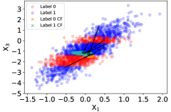
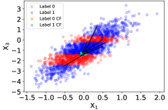
(a) CF-VAE	(b) EB-VAE

(c) Ours

Figure 3: Visualization of related variables of the synthetic toy dataset. The arrows indicate the directions from true samples to counterfactuals. CF means the generated counterfactuals.

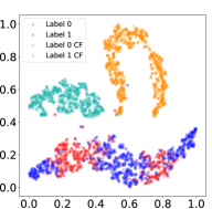
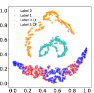
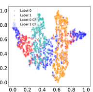
(a) CF-VAE	(b) EB-VAE	(c) Ours

Figure 4: $t$-SNE visualization of synthetic toy dataset.

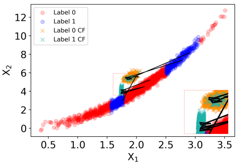
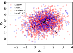
(a) CF-VAE

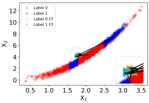
(b) EB-VAE

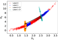
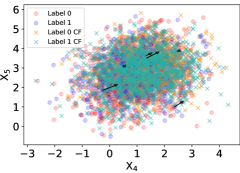
(c) Ours

Figure 5: The visualization related variables in synthetic non-linear dataset.

Synthetic 5-variable Non-linear Dataset. This dataset includes more complex and non-linear relationships between variables. The SEM are as follows:

$$X_{1} =U_{1} \quad\quad\quad U_{1} \sim\mathcal{N}(2,0.5)$$ (21)

$$X_{2} =X_{1}^{2}+U_{2} U_{2} \sim\mathcal{N}(0,0.25)$$ (22)

$$X_{3} =\texttt{sin}(-2X_{1})+U_{3} U_{3} \sim\mathcal{N}(0,1)$$ (23)

$$X_{4} =U_{4} U_{4} \sim\mathcal{N}(1,1)$$ (24)

$$X_{5} =\frac{1}{\texttt{e}^{-1.5X_{4}}}+2+U_{5} U_{5} \sim\mathcal{N}(0,1)$$ (25)

The dataset contains 20000 samples, and is split into training, validation and testing sets following the 8:1:1 ratio. The samples are labeled to 1 when $\texttt{sin}(X_{i})>0$ for all the 5 variables (without added Gaussian noise). This dataset includes two relationship constraints: (1) If absolute values of $X_{1}$ increase/decrease, $X_{2}$ increase/decrease, and (2) if $X_{4}$ increase/decrease, $X_{5}$ increase/decrease.

Summarized results are presented in the right half of Table 2. The results are similar to that of synthetic toy dataset. All the models except the Plain-CF generate counterfactuals with almost 100% valid labels. Our method has the highest constraint feasibility score indicating that our method preserves the relationships between the attributes. The distributions of the generated and the original samples are shown in Figure 5. Compared to other models, the counterfactuals generated by the proposed model has a larger intersection with the original sample distributions of the corresponding class. By comparing the arrows indicating the direction of the changes between the original samples and their corresponding counterfactuals, we observe that for the baseline methods, the samples tend to cluster into a small group and ignore the relationships. This is especially true for the pair $X_{4}$ and $X_{5}$. Our method, on the other hand, preserves the relationships. Having said that, all methods fail in capturing the non-linear relationships, however our method performs better than the compared methods.

Table 3: Experimental results on Sangiovese.

Methods	Valid (%)	Const (%)	Euclidean Dist	Mahalanobis Dist
Plain-CF	100	30.52	0.2821	6.2232
Plain-CFK	100	63.17	0.2665	5.0929
CF-VAE	99.84	63.03	0.2169	4.7695
EB-VAE	99.97	67.19	0.1857	3.6738
Ours	99.98	99.69	0.1961	1.9971

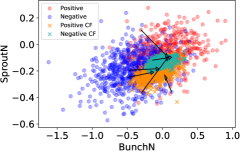
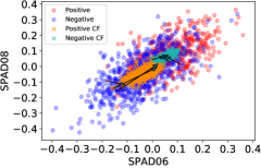
(a) CF-VAE

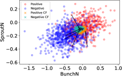
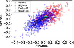
(b) EB-VAE

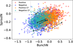
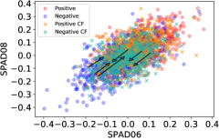
(c) Ours

Figure 6: Visualization of related variables in Sangiovese. Positive and negative indicate the predictions.

Simulated Bayesian Network Dataset. The dataset includes 10000 samples with 14 features and a categorical output for quality. We follow the data splitting setting in Mahajan et al. (2019). We measure two monotonic relationships (1) between SproutN and BunchN where if SproutN increases/decreases, BunchN increases/decreases; (2) between SPAD06 and SPAD08, where the same trend hold.

The quantitative results are shown in Table 3. As previously, the models achieve around near 100% validity. Our model is the second best in terms of Euclidean distance. However, in terms of Mahalanobis distance, our method has outperformed other methods. Besides, the constraint feasibility score of our method is nearly 100%, indicating the model perfectly captures the correlations between the variables. Figure 6 shows that the counterfactuals generated by EB-VAE of both labels tend to cluster together while the proposed model still keeps a clear boundary between the sets. Most of the changes that samples undergo in order to flip the labels are along the direction representing the relationship between the attributes.

4.3 Results on Diabetes Dataset (RQ2)

Dataset description. The dataset collected by Smith et al. (1988) contains medical records for Pima Indians with and without diabetes. Overall, the dataset contains 768 records, out of which 268 are diabetic and 500 are not. The records that contained missing values were removed, resulting in 336 records. Each record consists of 8 attributes. We selected the following 7: number of times pregnant, plasma glucose concentration at 2 hours in an oral glucose tolerance test, diastolic blood pressure, triceps skin fold thickness, 2-hour serum insulin, body mass index (BMI), and age. The target variable is the patients’ diabetic conditions i.e. positive (diabetic) or negative (not).

Before proceeding to generating and testing counterfactuals, we first conducted a qualitative analysis of the dataset in order to compare the observed relationships to prior domain knowledge on diabetes. Diabetes is a disease that is caused by either pancreas not being able to produce enough insulin or by organism not being able to use the produced insulin. Figure 7 shows pairwised correlations, it is easy to see that most pairs exhibit positive correlation. In particular, there is a strong linear relationship between insulin and glucose and hence in order to change the label from positive to negative, both glucose and insulin should be decreased. Further, it is easy to observe that besides having thinner skin, young people are less likely to be diabetic, and hence the counterfactuals that flip patients with diabetes to healthy might require to decrease their age. Given that decreasing age is infeasible, the changes that decrease the age are penalised. This prior expert knowledge is important in order to generate meaningful counterfactuals. It is also known that blood pressure and BMI are positively correlated, which is also observed in the chart ($\rho=0.27$). Interestingly, the number of pregnancies is correlated with blood pressure($\rho=0.3$), moreover women with a larger number of pregnancies are slightly more likely to have diabetes, which implies that the counterfactual might result in a decreased number of pregnancies in order to flip the predicted label from diabetic to healthy, such changes should also be penalised. Another interesting aspect that follows from the analysis of figure 7 is that blood pressure does not well separate healthy cohort and patients with diabetes, and hence should not undergo a significant change in the generated counterfactual compared to the original sample.

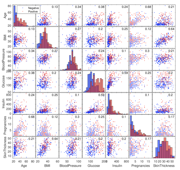
Figure 7: Visualization of paired attributes with correlations shown in top-right corners of corresponding panes. The positive class (red) indicates the diabetic patients while the negative (blue) is healthy.

We measure the constraint feasibility score by the pairs of blood pressure and BMI since from the domain knowledge we know that blood pressure and BMI are positively correlated ($\rho=0.27$), and hence in a counterfactual, the blood pressure and BMI should both increase or decrease. Since the number of samples is small, we use leave-one-out algorithm, which takes one sample for testing the model, while the rest of samples are used in training, this procedure is repeated over all samples, and an average accuracy is computed.

The quantitative evaluations are presented in Table 4.3. The validity for the methods are all nearly 100% and is not informative so we did not put them in the table. As it can be seen, around 74% of the counterfactuals satisfy the positive relationship between blood pressure and BMI. While the best baseline method attains about 60% counterfactuals that satisfy the relationship. The Mahalanobis distance of our method are significantly smaller than those of all the other baseline models. To qualitatively compare the methods, we plotted the counterfactuals on the blood pressure vs BMI (fig. 8). Given that blood pressure and BMI are positively correlated, we expected the counterfactuals to maintain this linear relationship, and hence the changes in these attributes should be along the direction representing the correlation. While our model maintained the correlation, the generated counterfactuals for other baselines, did not preserve the correlation, qualitatively demonstrating the efficiency of our method in learning the internal relationships between the two attributes and generating proper counterfactuals. It should also be noted that the class label could flip due to the change in other patient’s characteristic while keeping blood pressure and BMI constant.

Table 4: Results on Diabetes dataset.

Methods	Valid (%)	Cont (%)	Euclidean Dist	Mahalanobis Dist
CF-VAE	97.70	58.16	0.1288	3.2385
EB-VAE	99.74	60.97	0.1337	3.3189
Ours	99.74	88.44	0.1279	2.4042

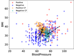
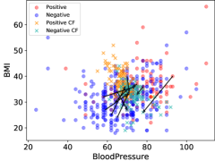
(a) CF-VAE	(b) EB-VAE

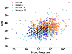
(c) Ours

Figure 8: Visualization of baseline and our method on diabetes dataset. Positive CF indicates the generated counterfactuals which are predicted to have diabetes while negative CF indicates counterfactuals which are predicted to be healthy.

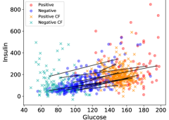
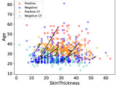
Figure 9: Visualization of some paired attributes in our method.

We further provide two examples of generated counterfactuals (table 5) in order to demonstrate a use-case of our model being useful in consulting patients. In both examples, our model suggests to decrease glucose and insulin, following our domain knowledge that glucose directly contributes to diabetes. Besides, it can be observed that the blood pressure, and skin thickness do decrease, which matches our observations in figure 7, as again, blood pressure and skin thickness seem to be associated with diabetes and correlated with each other ($\rho=0.21$). Similarly, the decrease in both blood pressure and BMI, demonstrates that the model learns the correlation between the two attributes as well as their associations with diabetes. This insight could be used by medical experts to provide medical advice to the patients. Example 2 illustrates a limitation of our method. The model suggests reducing age, even though a constraint was added to penalise unacceptable changes. In particular, nearly a third of the counterfactuals are generated with a slightly decreased age. This is especially true for counterfactuals flipping diabetes to healthy. We see that in generating counterfactuals for healthy, about 88% of the counterfactuals chose to increase the age. However, for diabetic counterfactuals, almost all counterfactuals resulted in a decreased age. The model often generates such counterfactuals due to a strong correlation between age and the target value i.e. young people are less likely to have diabetes (fig. 7). Since the objective of this paper is to study the relationships between attributes, we will leave the unary (attribute that can only change in one direction) constraint for future work.

To summarize, our method successfully captures the relationship between attributes (specifically the blood pressure and BMI). The generated counterfactuals preserve the relations that exist in the data and can be a good reference to suggest a patient what needs to be changed to become healthy. While we found age and pregnancies sometimes decrease, we will leave it to future work and constrain the changes so that such attributes should either stay constant or could only change in one direction.

Table 5: Examples of explanations with our method on Diabete dataset.

Attributes	Pregnancies	Glucose	Blood Pressure	Skinthickness	Insulin	BMI	Age	Diabetic
Original Input	1	166	73	17	144	23	33	Yes
Counterfactual	1	113	54	7	13	18	34	No
Original Input	0	134	93	46	145	40	26	Yes
Counterfactual	0	73	89	42	106	38	18	No

5 Conclusion and Future Work

In this paper, we proposed a novel method for generating counterfactuals that preserves the relationships between variables learned from data. A VAE was trained to reconstruct input vectors. Then a modulation network was trained to perturb the latent space representations such that counterfactuals are generated in place of input vectors. We experimented with synthetic and real datasets. The results show the superiority of the proposed method in generating realistic counterfactual explanations that preserve relationships while explaining machine learning models.

The proposed approach can be further extended as follows: (1) While we considered only binary classification tasks, it is of practical importance to extend the proposed model in a more complex multiple-label settings. (2) The model could further be modified to generate several counterfactual from a single sample by adding Gaussian noise to the latent space. (3) From a practical perspective, we plan to apply the proposed model to datasets of electronic medical records of patients with various diseases. The proposed model will provide medical experts with counterfactual explanations that will help patients to make necessary but minimal changes in either their lifestyles or treatments to further improve a probability of a positive health outcome.

References

- Štrumbelj and Kononenko [2014] Erik Štrumbelj and Igor Kononenko. Explaining prediction models and individual predictions with feature contributions. Knowledge and Information Systems, 41(3):647–665, 2014.
- Datta et al. [2016] Anupam Datta, Shayak Sen, and Yair Zick. Algorithmic transparency via quantitative input influence: Theory and experiments with learning systems. In 2016 IEEE Symposium on Security and Privacy (SP), pages 598–617, 2016.
- Ribeiro et al. [2016] Marco Túlio Ribeiro, Sameer Singh, and Carlos Guestrin. “why should i trust you?”: Explaining the predictions of any classifier. In Proceedings of the 2016 Conference of the North American Chapter of the Association for Computational Linguistics: Demonstrations, pages 97–101, 2016.
- Lundberg and Lee [2017] Scott M. Lundberg and Su-In Lee. A unified approach to interpreting model predictions. In NIPS’17 Proceedings of the 31st International Conference on Neural Information Processing Systems, volume 30, pages 4768–4777, 2017.
- Verma et al. [2020] Sahil Verma, John P. Dickerson, and Keegan Hines. Counterfactual explanations for machine learning: A review. arXiv preprint arXiv:2010.10596, 2020.
- Wachter et al. [2018] Sandra Wachter, Brent Mittelstadt, and Christopher Russell. Counterfactual explanations without opening the black box: Automated decisions and the gdpr. Harvard Journal of Law and Technology, 31(2):841, 2018.
- Dandl et al. [2020] Susanne Dandl, Christoph Molnar, Martin Binder, and Bernd Bischl. Multi-objective counterfactual explanations. In International Conference on Parallel Problem Solving from Nature, pages 448–469, 2020.
- Karimi et al. [2020] Amir-Hossein Karimi, Gilles Barthe, Borja Balle, and Isabel Valera. Model-agnostic counterfactual explanations for consequential decisions. In International Conference on Artificial Intelligence and Statistics, pages 895–905, 2020.
- Mahajan et al. [2019] Divyat Mahajan, Chenhao Tan, and Amit Sharma. Preserving causal constraints in counterfactual explanations for machine learning classifiers. arXiv preprint arXiv:1912.03277, 2019.
- Karimi et al. [2020] Amir-Hossein Karimi, Bernhard Schölkopf, and Isabel Valera. Algorithmic recourse: from counterfactual explanations to interventions. arXiv preprint arXiv:2002.06278, 2020.
- Karimi et al. [2020] Amir-Hossein Karimi, Bodo Julius von Kügelgen, Bernhard Schölkopf, and Isabel Valera. Algorithmic recourse under imperfect causal knowledge: a probabilistic approach. In Advances in Neural Information Processing Systems, volume 33, 2020.
- Downs et al. [2020] Michael Downs, Jonathan L Chu, Yaniv Yacoby, Finale Doshi-Velez, and Weiwei Pan. Cruds: Counterfactual recourse using disentangled subspaces. In ICML Workshop on Human Interpretability in Machine Learning, 2020.
- Pearl et al. [2016] Judea Pearl, Madelyn Glymour, and Nicholas P. Jewell. Causal inference in statistics : a primer. 2016.
- Yu et al. [2019] Yue Yu, Jie Chen, Tian Gao, and Mo Yu. Dag-gnn: Dag structure learning with graph neural networks. In International Conference on Machine Learning, pages 7154–7163, 2019.
- Peters et al. [2017] Jonas Peters, Dominik Janzing, and Bernhard Schlkopf. Elements of Causal Inference: Foundations and Learning Algorithms. The MIT Press, 2017.
- Spirtes et al. [2000] Peter Spirtes, Clark N Glymour, Richard Scheines, and David Heckerman. Causation, prediction, and search. MIT press, 2000.
- Mooij et al. [2016] Joris M Mooij, Jonas Peters, Dominik Janzing, Jakob Zscheischler, and Bernhard Schölkopf. Distinguishing cause from effect using observational data: methods and benchmarks. The Journal of Machine Learning Research, 17(1):1103–1204, 2016.
- Glymour et al. [2019] Clark Glymour, Kun Zhang, and Peter Spirtes. Review of causal discovery methods based on graphical models. Frontiers in genetics, 10:524, 2019.
- Zhu et al. [2020] Shengyu Zhu, Ignavier Ng, and Zhitang Chen. Causal discovery with reinforcement learning. In ICLR 2020 : Eighth International Conference on Learning Representations, 2020.
- Kingma and Welling [2014] Diederik P Kingma and Max Welling. Auto-encoding variational bayes. In ICLR 2014 : International Conference on Learning Representations (ICLR) 2014, 2014.
- Albini et al. [2020] Emanuele Albini, Antonio Rago, Pietro Baroni, and Francesca Toni. Relation-based counterfactual explanations for bayesian network classifiers. In IJCAI, pages 451–457, 2020.
- Kommiya Mothilal et al. [2021] Ramaravind Kommiya Mothilal, Divyat Mahajan, Chenhao Tan, and Amit Sharma. Towards unifying feature attribution and counterfactual explanations: Different means to the same end. In Proceedings of the 2021 AAAI/ACM Conference on AI, Ethics, and Society, pages 652–663, 2021.
- Parmentier and Vidal [2021] Axel Parmentier and Thibaut Vidal. Optimal counterfactual explanations in tree ensembles. In International Conference on Machine Learning, pages 8422–8431. PMLR, 2021.
- Mothilal et al. [2020] Ramaravind K Mothilal, Amit Sharma, and Chenhao Tan. Explaining machine learning classifiers through diverse counterfactual explanations. In Proceedings of the 2020 Conference on Fairness, Accountability, and Transparency, pages 607–617, 2020.
- Grath et al. [2018] Rory Mc Grath, Luca Costabello, Chan Le Van, Paul Sweeney, Farbod Kamiab, Zhao Shen, and Freddy Lecue. Interpretable credit application predictions with counterfactual explanations. arXiv preprint arXiv:1811.05245, 2018.
- Keane and Smyth [2020] Mark T Keane and Barry Smyth. Good counterfactuals and where to find them: A case-based technique for generating counterfactuals for explainable ai (xai). In International Conference on Case-Based Reasoning, pages 163–178. Springer, 2020.
- Ferrario and Loi [2020] Andrea Ferrario and Michele Loi. A series of unfortunate counterfactual events: the role of time in counterfactual explanations. arXiv preprint arXiv:2010.04687, 2020.
- Koivisto and Sood [2005] Mikko Koivisto and Kismat Sood. Exact bayesian structure discovery in bayesian networks. Journal of Machine Learning Research, 5:549–573, 2005.
- Sohn et al. [2015] Kihyuk Sohn, Xinchen Yan, and Honglak Lee. Learning structured output representation using deep conditional generative models. In NIPS’15 Proceedings of the 28th International Conference on Neural Information Processing Systems - Volume 2, volume 28, pages 3483–3491, 2015.
- Makhzani et al. [2015] Alireza Makhzani, Jonathon Shlens, Navdeep Jaitly, Ian Goodfellow, and Brendan Frey. Adversarial autoencoders. arXiv preprint arXiv:1511.05644, 2015.
- Smith et al. [1988] Jack W Smith, James E Everhart, WC Dickson, William C Knowler, and Robert Scott Johannes. Using the adap learning algorithm to forecast the onset of diabetes mellitus. In Proceedings of the annual symposium on computer application in medical care, page 261. American Medical Informatics Association, 1988.