User-Oriented Robust Reinforcement Learning

Abstract

Recently, improving the robustness of policies across different environments attracts increasing attention in the reinforcement learning (RL) community. Existing robust RL methods mostly aim to achieve the max-min robustness by optimizing the policy’s performance in the worst-case environment. However, in practice, a user that uses an RL policy may have different preferences over its performance across environments. Clearly, the aforementioned max-min robustness is oftentimes too conservative to satisfy user preference. Therefore, in this paper, we integrate user preference into policy learning in robust RL, and propose a novel User-Oriented Robust RL (UOR-RL) framework. Specifically, we define a new User-Oriented Robustness (UOR) metric for RL, which allocates different weights to the environments according to user preference and generalizes the max-min robustness metric. To optimize the UOR metric, we develop two different UOR-RL training algorithms for the scenarios with or without a priori known environment distribution, respectively. Theoretically, we prove that our UOR-RL training algorithms converge to near-optimal policies even with inaccurate or completely no knowledge about the environment distribution. Furthermore, we carry out extensive experimental evaluations in 6 MuJoCo tasks. The experimental results demonstrate that UOR-RL is comparable to the state-of-the-art baselines under the average-case and worst-case performance metrics, and more importantly establishes new state-of-the-art performance under the UOR metric.

1 Introduction

Recently, reinforcement learning (RL) raises a high level of interest in both the research community and the industry due to its satisfactory performance in a variety of decision-making tasks, such as playing computer games [1], autonomous driving [2], robotics [3]. Among existing RL methods, model-free ones, such as DQN [1], DDPG [4], PPO [5], which typically train policies in simulated environments, have been widely studied. However, it is highly possible that there exist discrepancies between the training and execution environments, which could severely degrade the performance of the trained policies. Therefore, it is of significant importance to robustify RL policies across different environments.

Existing studies of RL robustness against environment discrepancies [6, 7, 8, 9] mostly aim to achieve the max-min robustness by optimizing the performance of the policy in the worst-case environment. However, such max-min robustness could oftentimes be overly conservative, since it only concentrates on the performance of the policy in the worst case, regardless of its performance in any other case. As a matter of fact, it is usually extremely rare for the worst case (e.g., extreme weather conditions in autonomous driving, power failure incidence in robot control) to happen in many applications. Therefore, we should take the environment distribution into consideration and pay more attention to the environments with higher probabilities though they are not the worst.

Besides, a user that uses an RL policy for real-world tasks may have different preferences over her performance across environments. Furthermore, for the same decision-making task, the preferences of different users may vary, resulting that they are in favor of different policies. For instance, in computer games, some users prefer to attack others and take an aggressive policy, while others may prefer a defensive policy. Therefore, user preference is a crucial factor that should be considered in RL policy training, which is ignored by the max-min robustness.

Due to the significance of user preference and environment distribution, we design a new User-Oriented Robustness (UOR) metric, which integrates both user preference and environment distribution into the measurement of robustness. Specifically, the UOR metric allocates different weights to different environments, based on user preference, environment distribution, and relative policy performance. In fact, the max-min robustness is a special case of the UOR metric that the user prefers extremely conservative robustness, and thus, the UOR metric is a generalization of the max-min robustness. Hence, in this paper, we focus on optimizing the UOR metric during policy training, which can help obtain policies better aligned with user preference.

To optimize the UOR metric, we propose the User-Oriented Robust RL (UOR-RL) framework. One of the training algorithms of the UOR-RL framework, namely Distribution-Based UOR-RL (DB-UOR-RL), takes the environment distribution as input to help optimize the UOR metric. In real-world applications, however, the environment distribution may sometimes be unknown to the user. To tackle such case, we design another training algorithm, namely Distribution-Free UOR-RL (DF-UOR-RL), which works even without any knowledge of the environment distribution. Both algorithms evaluate the UOR metric and use it to update the policy, while they differ in their approaches for UOR metric evaluation, because of the different prior knowledge of the environment distribution.

Theoretically, under several mild assumptions, we prove that UOR-RL guarantees the following series of desirable properties. For DB-UOR-RL, we prove that with $O(\frac{1}{\epsilon^{d}})$ computational complexity, where $d$ denotes the dimension of the parameter that parameterizes the environment, the output policy of DB-UOR-RL is $\epsilon$-suboptimal to the optimal policy under the UOR metric. Furthermore, even when DB-UOR-RL takes an inaccurate empirical environment distribution as input, we prove that, as long as the total variation distance between the empirical distribution and the accurate one is no larger than $O(\epsilon^{d})$, the output policy of DB-UOR-RL is still guaranteed to be $\epsilon$-suboptimal to the optimal policy. For DF-UOR-RL, though without any prior knowledge of the environment distribution, our proof shows that DF-UOR-RL could still generate an $\epsilon$-suboptimal policy with $O(\frac{1}{\epsilon^{2d+4}})$ computational complexity.

The contributions of this paper are summarized as follows.

• We propose a user-oriented metric for robustness measurement, namely UOR, allocating different weights to different environments according to user preference. To the best of our knowledge, UOR is the first metric that integrates user preference into the measurement of robustness in RL.

• We design two UOR-RL training algorithms for the scenarios with or without a priori known environment distribution, respectively. Both algorithms take the UOR metric as the optimization objective so as to obtain policies better aligned with user preference.

• We prove a series of results, through rigorous theoretical analysis, showing that our UOR-RL training algorithms converge to near-optimal policies even with inaccurate or entirely no knowledge about the environment distribution.

• We conduct extensive experiments in 6 MuJoCo tasks. The experimental results demonstrate that UOR-RL is comparable to the state-of-the-art baselines under the average-case and worst-case performance metrics, and more importantly establishes new state-of-the-art performance under the UOR metric.

2 Problem Statement

2.1 Preliminary

We introduce parameterized Markov Decision Process (PMDP) [7] represented by a 6-tuple $(\mathcal{S},\mathcal{A},\gamma,\mathbb{S}_{0},T,R)$, as it is the basis of the UOR-PMDP that will be defined in Section 2.2. $\mathcal{S}$ and $\mathcal{A}$ are respectively the set of states and actions. $\gamma$ is the discount factor. $\mathbb{S}_{0}\in\Delta(\mathcal{S})$ denotes the initial state distribution. Furthermore, different from the traditional MDP, a PMDP’s transition function $T:\mathcal{S}\times\mathcal{A}\times\mathcal{P}\rightarrow\Delta(\mathcal{S})$ and reward function $R:\mathcal{S}\times\mathcal{A}\times\mathcal{S}\times\mathcal{P}\rightarrow\Delta(\mathbb{R})$ take an additional environment parameter $p$ as input, with $\mathbb{R}$ denoting the set of all real numbers. The environment parameter $p$ is a random variable in range $\mathcal{P}\subset\mathbb{R}^{d}$, following a probability distribution $\mathbb{D}$. In PMDP, the parameter $p$ is sampled at the beginning of each trajectory, and keeps constant during the trajectory. We consider the scenario where $p$ is unknown to the user during execution, but our work can extend to the scenario with known $p$ through regarding the environment parameter $p$ as an additional dimension of state.

A policy $\pi:\mathcal{S}\rightarrow\Delta(\mathcal{A})$ is a mapping from a state to a probability distribution over actions. Furthermore, the expected return $J(\pi,p)$ is defined as the expected discounted sum of rewards when the policy $\pi$ is executed under the environment parameter $p$, i.e.,

$$J(\pi,p)=\mathbb{E}\left[\sum_{t=0}^{\infty}\gamma^{t}R(s_{t},a_{t},s_{t+1},p)|\pi\right].$$ (1)

2.2 User-Oriented Robust PMDP

Definition

In this paper, we propose User-Oriented Robust PMDP (UOR-PMDP), which is represented by an 8-tuple $(\mathcal{S},\mathcal{A},\gamma,\mathbb{S}_{0},T,R,h,W)$. The first six items of UOR-PMDP are the same as those of PMDP. Furthermore, we introduce the last two items, namely the ranking function $h$ and the preference function $W$, to formulate our new User-Oriented Robustness (UOR) metric that allocates more weights to the environment parameters where the policy has relatively worse performance, according to user preference.

As UOR requires assessing the relative performance of the policy under different environment parameters, we define the ranking function $h:\Pi\times\mathcal{P}\rightarrow[0,1]$ as

$$h(\pi,p)=\int_{\mathcal{P}}\mathbb{D}(p)\cdot\mathds{1}\left[J(\pi,p^{\prime})\leq J(\pi,p)\right]\mathrm{d}p^{\prime},$$ (2)

which represents the probability that the performance of policy $\pi$ under an environment parameter $p^{\prime}$ sampled from $\mathbb{D}$ is worse than that under the environment parameter $p$.

To represent a user’s preference, we define the preference function $W:[0,1]\rightarrow\mathbb{R_{+}}\cup\{0\}$ which assigns weights to environment parameters with different rankings. Specifically, given $\pi$, the weight assigned to environment parameter $p$ is set as $W(h(\pi,p))$. Moreover, we require function $W$ to be non-increasing, since UOR essentially puts more weights on environment parameters with lower rankings.

In practice, to make it more convenient for a user to specify her preference, we could let the preference function $W$ belong to a family of functions parameterized by as few as only one parameter. For example, by setting the preference function $W$ as

$$W(x)=(k+1)\cdot(1-x)^{k},$$ (3)

a single robustness degree parameter $k\in\mathbb{R_{+}}$ suffices to completely characterize the user preference.

In terms of the objective, the UOR-PMDP aims to maximize the UOR metric $\mathcal{E}$ defined as

$$\mathcal{E}(\pi)=\int_{\mathcal{P}}\mathbb{D}(p)\cdot J(\pi,p)\cdot W(h(\pi,p))\mathrm{d}p,$$ (4)

which is the expectation of the weighted sum of $J(\pi,p)$ over the distribution $\mathbb{D}$. That is, the optimal policy $\pi^{\ast}$ of the UOR-PMDP satisfies

$$\pi^{\ast}=\operatorname*{arg\,max}_{\pi\in\Pi}\mathcal{E}(\pi).$$ (5)

Properties

In fact, our UOR metric generalizes the worst-case performance robustness metric $\min_{p\in\mathcal{P}}J(\pi,p)$ [6, 7, 8, 9], and the average-case metric $\mathbb{E}_{p\sim\mathbb{D}}\left[J(\pi,p)\right]$ without robustness consideration [10, 11].

As $W$ is non-increasing, it has the following two extreme cases. For one extreme case, $W$ concentrates on zero. That is, $W(x)=\delta(x)$, where $\delta$ denotes the Dirac function, and consequently the UOR metric becomes

$$\mathcal{E}(\pi)=\int_{\mathcal{P}}\mathbb{D}(p)\cdot J(\pi,p)\cdot\delta(h(\pi,p))\mathrm{d}p=\min_{p\in\mathcal{P}}J(\pi,p).$$

For the other extreme case, $W$ is uniform in $[0,1]$. That is, $W(x)\equiv 1$, and consequently the UOR metric becomes

$$\mathcal{E}(\pi)=\int_{\mathcal{P}}\mathbb{D}(p)\cdot J(\pi,p)\mathrm{d}p=\mathbb{E}_{p\sim\mathbb{D}}\left[J(\pi,p)\right].$$

3 Solutions for UOR-PMDP

In this section, we present two User-Oriented Robust RL (UOR-RL) algorithms to solve UOR-PMDP in the scenarios with and without a priori known environment parameter distribution, respectively.

3.1 Distribution-Based UOR-RL

Algorithm Design

We consider the scenario that the distribution $\mathbb{D}$ is known before training, and propose the Distribution-Based UOR-RL (DB-UOR-RL) training algorithm in Algorithm 1 which makes use of the distribution $\mathbb{D}$ during the training period.

// Initialization.

1 Initialize policy $\pi_{\theta^{0}}$ and block diameter upper bound $\delta$;

2 $\{\mathcal{P}_{1},\mathcal{P}_{2},\cdots,\mathcal{P}_{n}\}\leftarrow\text{Set\_Division}(\mathcal{P},\delta)$;

3 foreach Block $\mathcal{P}_{j}$ do

4       $p_{j}\leftarrow$ Arbitrarily chosen element in $\mathcal{P}_{j}$;

5       $m_{j}\leftarrow\int_{\mathcal{P}_{j}}\mathbb{D}(p)\mathrm{d}p$;

6      

// Policy Training.

7 foreach Iteration $i=0$ to max-iterations do

8       foreach Block $\mathcal{P}_{j}$ do

9            

10            Execute policy $\pi_{\theta^{i}}$ under $p_{j}$ and evaluate the empirical expected return $\hat{J}(\pi_{\theta^{i}},p_{j})$;

11            

12      Sort the sequence $\{\hat{J}(\pi_{\theta^{i}},p_{j})\}$ into an increasing sequence $\{\hat{J}(\pi_{\theta^{i}},p_{\alpha_{j}})\}$;

       // Metric Calculation.

13       Initialize metric $\hat{\mathcal{E}}(\pi_{\theta^{i}})\leftarrow 0$ and $M\leftarrow 0$;

14       foreach Block $\mathcal{P}_{j}$ do

15             $w_{j}\leftarrow\int_{M}^{M+m_{\alpha_{j}}}W(x)\mathrm{d}x$;

16             $\hat{\mathcal{E}}(\pi_{\theta^{i}})\leftarrow\hat{\mathcal{E}}(\pi_{\theta^{i}})+w_{j}\cdot\hat{J}(\pi_{\theta^{i}},p_{\alpha_{j}})$;

17             $M\leftarrow M+m_{\alpha_{j}}$;

18            

      // Policy Update.

19       $\pi_{\theta^{i+1}}\leftarrow$ Policy_Update$(\pi_{\theta^{i}},\hat{\mathcal{E}}(\pi_{\theta^{i}}))$;

20      

ALGORITHM 1 DB-UOR-RL Algorithm

Firstly, Algorithm 1 randomly sets the initial policy $\pi_{\theta^{0}}$, and chooses the upper bound $\delta$ of the block diameter (line 1). The criteria for setting $\delta$ will be discussed in detail in Section 3.1. Then, by calling the Set_Division algorithm, Algorithm 1 divides $\mathcal{P}$ into $n$ blocks $\mathcal{P}_{1},\mathcal{P}_{2},\cdots,\mathcal{P}_{n}$, whose diameters are less than $\delta$ (line 1). That is,

$$\forall~{}\mathcal{P}_{j}\in\{\mathcal{P}_{1},\mathcal{P}_{2},\cdots,\mathcal{P}_{n}\},\forall~{}p_{x},p_{y}\in\mathcal{P}_{j},||p_{x}-p_{y}||_{2}\leq\delta.$$

Note that the number of blocks $n$ is decided by how the Set_Division algorithm divides $\mathcal{P}$ based on $\delta$. Because of space limit, we put our Set_Division algorithm in Appendix B. In fact, Algorithm 1 works with any Set_Division algorithm that could guarantee that the diameters of the divided blocks are upper bounded by $\delta$. Then, for each block $\mathcal{P}_{j}$, Algorithm 1 arbitrarily chooses an element $p_{j}$ from the block to represent it (line  1), and calculates the probability that an environment parameter falls into the block $\mathcal{P}_{j}$ (line  1).

Next, Algorithm 1 trains the policy (line 1 to 1). In each iteration $i$, it evaluates the performance $\hat{J}(\pi_{\theta^{i}},p_{j})$ of the policy $\pi_{\theta^{i}}$ under each $p_{j}$ (line 1), and sorts the sequence $\{\hat{J}(\pi_{\theta^{i}},p_{j})\}$ into an increasing one $\{\hat{J}(\pi_{\theta^{i}},p_{\alpha_{j}})\}$ (line 1). Then, Algorithm 1 calculates the metric $\hat{\mathcal{E}}(\pi_{\theta^{i}})$, which is an approximation of the UOR metric $\mathcal{E}(\pi_{\theta^{i}})$ (line 1 to 1). Specifically, it initializes the metric $\hat{\mathcal{E}}(\pi_{\theta^{i}})$ and the lower limit $M$ of the integral as zero (line 1). For each block $\mathcal{P}_{j}$, it calculates the weight $w_{j}$ allocated to this block based on the ranking $\alpha_{j}$ of block $\mathcal{P}_{j}$ in the sorted sequence $\{J(\pi_{\theta^{i}},p_{\alpha_{j}})\}$ and preference function $W$ (line 1), and updates the metric $\hat{\mathcal{E}}(\pi_{\theta^{i}})$ (line 1) and the lower limit of the integral (line 1). Finally, based on the metric $\hat{\mathcal{E}}(\pi_{\theta^{i}})$, Algorithm 1 updates the policy by applying a Policy_Update algorithm (line 1). Note that Policy_Update could be any policy gradient algorithm that updates the policy based on the metric $\hat{\mathcal{E}}(\pi_{\theta^{i}})$.

The above Algorithm 1 essentially uses integral discretization to calculate an approximate UOR metric $\hat{\mathcal{E}}$ which is used as the optimization objective of Policy_Update. To discretize the integral for calculating the UOR metric, Algorithm 1 divides the environment parameter range into blocks. Furthermore, to get the ranking function for weight allocation, Algorithm 1 sorts the blocks according to the evaluated performance on them.

Algorithm Analysis

To analyze Algorithm 1, we make the following three mild assumptions.

Assumption 1.

The transition function $T$ and reward function $R$ are continuous to the environment parameter $p$.

Assumption 2.

The transition function $T$ and reward function $R$ are Lipschitz continuous to the state space $\mathcal{S}$ and action space $\mathcal{A}$ with constants $L_{T,\mathcal{S}}$, $L_{T,\mathcal{A}}$, $L_{R,\mathcal{S}}$, and $L_{R,\mathcal{A}}$, respectively.

Assumption 3.

The policy $\pi$ during the training process in Algorithm 1 is Lipschitz continuous with constant $L_{\pi}$.

Assumption 1 is natural, because the $R$ and $T$ functions characterize the environment which will usually not change abruptly as the environment parameter $p$ changes. Furthermore, Assumptions 2 and 3 are commonly used in previous works [12, 9]. Based on Assumptions 1-3, we prove the following Theorem 1, which demonstrates the existence of the diameter upper bound $\delta$ under which Algorithm 1 can converge to a near-optimal policy.

Theorem 1.

$\forall$ optimality requirement $\epsilon=2\epsilon_{0}>0$, $\exists~{}\delta_{0}$, such that as long as Policy_Update can learn an $\epsilon_{0}$-suboptimal policy for metric $\hat{\mathcal{E}}$, by running Algorithm 1 with any diameter upper bound $\delta\leq\delta_{0}$, we can guarantee that the output policy $\hat{\pi}$ of Algorithm 1 satisfies

$$\mathcal{E}(\hat{\pi})\geq\mathcal{E}(\pi^{\ast})-\epsilon.$$ (6)

Because of space limit, the proofs to all of the theorems and corollary in this paper are provided in the appendix.

Theorem 1 reveals that as long as the diameter upper bound $\delta$ is sufficiently small, the output policy $\hat{\pi}$ of Algorithm 1 will be close enough to the optimal policy $\pi^{\ast}$. However, as $\delta$ decreases, the number of the blocks output by Set_Division on line 1 of Algorithm 1 will increase, leading to an increased complexity of Algorithm 1. Thus, it is of great importance to have a quantitative relationship between $\epsilon$ and $\delta$, which could help us better choose the upper bound $\delta$ based on the optimality requirement $\epsilon$. To obtain the quantitative relationship between $\delta$ and $\epsilon$, we introduce the following Assumption 4, which is stronger than Assumption 1.

Assumption 4.

The transition function $T$ and reward function $R$ are Lipschitz continuous to the environment parameter $p$ with constants $L_{T,p}$ and $L_{R,p}$.

Based on Assumptions 2-4, we prove Theorem 2.

Theorem 2.

$\forall$ optimality requirement $\epsilon=2\epsilon_{0}>0$, $\exists~{}\delta_{0}=\upsilon\epsilon=O(\epsilon)$, such that as long as Policy_Update can learn an $\epsilon_{0}$-suboptimal policy for metric $\hat{\mathcal{E}}$, by running Algorithm 1 with any diameter upper bound $\delta\leq\delta_{0}$, we can guarantee that the output policy $\hat{\pi}$ of Algorithm 1 satisfies

$$\mathcal{E}(\hat{\pi})\geq\mathcal{E}(\pi^{\ast})-\epsilon.$$ (7)

Note that the constant $\upsilon$ depends on the Lipschitz constants in Assumptions 2-4, whose detailed form is presented in Equation (51) in Appendix A.2.

Theorem 2 indicates that when Algorithm 1 chooses $\delta=\upsilon\epsilon=O(\epsilon)$, the number of divided blocks is at most $O(\frac{1}{\epsilon^{d}})$. Therefore, with such choice of $\delta$, we can guarantee that the complexity of each iteration in Algorithm 1 is at most $O(\frac{1}{\epsilon^{d}})$.

In practice, the user may not know the accurate distribution $\mathbb{D}$, but only has access to a biased empirical distribution $\mathbb{D}^{e}$. In the following Theorem 3, we prove the theoretical guarantee of Algorithm 1 when it runs with $\mathbb{D}^{e}$.

Theorem 3.

Define the policy $\pi^{e}$ such that

$$\pi^{e}=\operatorname*{arg\,max}_{\pi}\mathcal{E}^{e}(\pi),$$ (8)

where $\mathcal{E}^{e}$ denotes the UOR metric under the UOR-PMDP with the empirical environment parameter distribution $\mathbb{D}^{e}$.

Then, $\forall$ given $\epsilon>0$, $\exists~{}\kappa=O(\epsilon^{d})$, such that as long as $\mathbb{D}$ and $\mathbb{D}^{e}$ satisfies the total variation distance $D_{TV}(\mathbb{D},\mathbb{D}^{e})\leq\kappa$, then we can guarantee that

$$\mathcal{E}(\pi^{e})\geq\mathcal{E}(\pi^{\ast})-\epsilon.$$ (9)

Based on Theorems 2 and 3, we have Corollary 10.

Corollary 1.

$\forall$ optimality requirement $\epsilon_{1}=3\epsilon>0$, $\exists~{}\delta_{0}=O(\epsilon)$ and $\kappa=O(\epsilon^{d})$, such that as long as $D_{TV}(\mathbb{D},\mathbb{D}^{e})\leq\kappa$ and Policy_Update can learn an $\epsilon$-suboptimal policy for metric $\hat{\mathcal{E}}$, by running Algorithm 1 with diameter upper bound $\delta\leq\delta_{0}$ and distribution $\mathbb{D}^{e}$, we can guarantee that the output policy $\hat{\pi}^{e}$ of Algorithm 1 satisfies

$$\mathcal{E}(\hat{\pi}^{e})\geq\mathcal{E}(\pi^{\ast})-\epsilon_{1}.\vspace{-0.8cm}$$ (10)

Corollary 10 demonstrates that even running Algorithm 1 with the biased distribution $\mathbb{D}^{e}$, as long as $\mathbb{D}^{e}$ is close enough to $\mathbb{D}$, the output policy is still near-optimal.

3.2 Distribution-Free UOR-RL

Algorithm design

In practice, it is likely that the distribution function $\mathbb{D}$ is unknown, making Algorithm 1 not applicable. Therefore, we propose the Distribution-Free UOR-RL (DF-UOR-RL) training algorithm in Algorithm 2 that trains a satisfactory policy even without any knowledge of the distribution function $\mathbb{D}$.

// Initialization

1 Initialize empty trajectory clusters $\mathcal{C}_{1},\mathcal{C}_{2},\cdots,\mathcal{C}_{n_{1}}$, cluster size $n_{2}$, and policy $\pi_{\theta^{0}}$;

// Policy Training

2 foreach Iteration $i=0$ to max-iterations do

3       foreach $j=1$ to $n_{1}$ do

4             foreach $k=1$ to $n_{2}$ do

5                   Observe environment parameter $p_{j,k}$;

6                   Execute $\pi_{\theta^{i}}$ under $p_{j,k}$, get trajectory $\xi_{j,k}$, and $\mathcal{C}_{j}\leftarrow\mathcal{C}_{j}\cup\{\xi_{j,k}\}$;

7                   Evaluate discounted reward $\hat{J}(\xi_{j,k})$ of $\xi_{j,k}$;

8                  

9            $\hat{J}_{j}\leftarrow\frac{1}{|\mathcal{C}_{j}|}\cdot\sum_{\xi_{j,k}\in\mathcal{C}_{j}}\hat{J}(\xi_{j,k})$;

10            

11      Sort the sequence $\{\hat{J}_{j}\}$ into an increasing sequence $\{\hat{J}_{\alpha_{j}}\}$;

       // Metric Calculation

12       Initialize metric $\tilde{\mathcal{E}}(\pi_{\theta^{i}})\leftarrow 0$;

13       foreach $j=1$ to $n$ do

14             $w_{j}\leftarrow\int_{(j-1)/n}^{j/n}W(x)\mathrm{d}x$;

15             $\tilde{\mathcal{E}}(\pi_{\theta^{i}})\leftarrow\tilde{\mathcal{E}}(\pi_{\theta^{i}})+w_{j}\cdot\hat{J}_{\alpha_{j}}$;

16            

      // Policy Update

17       $\pi_{\theta^{i+1}}\leftarrow$ Policy_Update$(\pi_{\theta^{i}},\tilde{\mathcal{E}}(\pi_{\theta^{i}}))$;

18      

ALGORITHM 2 DF-UOR-RL Algorithm

At the beginning, Algorithm 2 randomly sets the initial policy $\pi_{\theta^{0}}$ and $n_{1}$ empty clusters, and chooses the size of each cluster as $n_{2}$ (line 2). We will introduce in detail how to set the number of clusters $n_{1}$ and cluster size $n_{2}$ in Section 3.2. Then, Algorithm 2 begins to train the policy (line 2-2). In each iteration $i$, it samples $n_{2}$ trajectories for each cluster $\mathcal{C}_{j}$, by executing the current policy $\pi_{\theta^{i}}$ under the observed environment parameters (line 2-2), and evaluates the discounted reward of these trajectories (line 2). After that, Algorithm 2 evaluates the performance $\hat{J}_{j}$ of each cluster $\mathcal{C}_{j}$ by averaging the discounted reward of the trajectories in the cluster (line 2), and sorts the sequence $\{\hat{J}_{j}\}$ into an increasing one $\{\hat{J}_{\alpha_{j}}\}$ (line 2). Then, Algorithm 2 calculates the metric $\tilde{\mathcal{E}}(\pi_{\theta^{i}})$, which is an approximation of the UOR metric $\mathcal{E}(\pi_{\theta^{i}})$ (line 2-2). Initially, it sets the metric $\tilde{\mathcal{E}}(\pi_{\theta^{i}})$ as zero (line 2). Then, for each cluster $\mathcal{C}_{j}$, Algorithm 2 allocates the weight to cluster according to its ranking $\alpha_{j}$ and the preference function (line 2) and updates the $\tilde{\mathcal{E}}(\pi_{\theta^{i}})$ (line 2) based on the weight and performance of the cluster. Finally, Algorithm 2 obtains the $\tilde{\mathcal{E}}(\pi_{\theta^{i}})$ and uses it to update the policy (line 2).

Different from Algorithm 1, due to the lack of the knowledge of the distribution $\mathbb{D}$, Algorithm 2 observes the environment parameter rather than directly sample it according to $\mathbb{D}$. Given that it is of large bias to evaluate $J(\pi,p)$ from only one trajectory, Algorithm 2 averages the discounted rewards of $n_{2}$ trajectories. The clusters in Algorithm 2 have the same functionality as the blocks in Algorithm 1, and Algorithm 2 uses them to calculate an approximate UOR metric $\tilde{\mathcal{E}}(\pi_{\theta^{i}})$.

Algorithm Analysis

To analyze Algorithm 2, we introduce an additional mild Assumption 5 on two properties of the environment parameters, including the difference between consecutively sampled environment parameters in line 2 of Algorithm 2, and the convergence rate of the posterior distribution of the environment parameter to the distribution $\mathbb{D}$. Because of space limit, we provide the detailed description of Assumption  86 in Appendix 82.

Based on Assumptions 2-86, we have the theoretical guarantee of Algorithm 2 in the following Theorem 4.

Theorem 4.

$\forall$ optimality requirement $\epsilon=2\epsilon_{0}>0$ and confidence $\rho$, $\exists~{}n_{1}=\Theta(\frac{-\ln\rho}{\epsilon^{2}}),n_{2}=\Theta(\frac{-\ln\rho}{\epsilon^{2d+2}})$, such that as long as Policy_Update can learn an $\epsilon_{0}$-suboptimal policy for metric $\tilde{\mathcal{E}}$, by running Algorithm 2 with trajectory cluster number larger than $n_{1}$ and cluster size larger than $n_{2}$, we can guarantee that the output policy $\tilde{\pi}$ of Algorithm 2 satisfies

$$\mathcal{E}(\pi)\geq\mathcal{E}(\tilde{\pi})-\epsilon$$ (11)

with confidence more than $1-\rho$.

Theorem 4 provides guidelines for setting the cluster size $n_{1}$ and cluster number $n_{2}$ in Algorithm 2. In fact, as $n_{1}$ and $n_{2}$ increase, the performance evaluation of the cluster and the weight allocated to the cluster will be more accurate, both of which lead to a more accurate approximation of the UOR metric. However, the increase of either $n_{1}$ or $n_{2}$ leads to an increased complexity of each iteration of Algorithm 2. To deal with such trade-off, we could set $n_{1}$ and $n_{2}$ based on the lower bounds in Theorem 4, through which Algorithm 2 can guarantee both the optimality requirement $\epsilon$ and $O(\frac{\ln^{2}{\rho}}{\epsilon^{2d+4}})$ complexity of each iteration.

4 Experiments

4.1 Baseline Methods

We compare UOR-RL with the following four baselines.
Domain Randomization-Uniform (DR-U). Domain Randomization (DR) [11] is a method that randomly samples environment parameters in a domain, and optimizes the expected return over all collected trajectories. DR-U is an instance of DR, which samples environment parameters from a uniform distribution. Domain Randomization-Gaussian (DR-G). DR-G is another instance of DR, which samples environment parameters from a Gaussian distribution. Ensemble Policy Optimization (EPOpt). EPOpt [7] is a method that aims to find a robust policy through optimizing the performance of the worst few collected trajectories. Monotonic Robust Policy Optimization (MRPO). MRPO [13] is the state-of-the-art robust RL method, which is based on EPOpt and jointly optimizes the performance of the policy in both the average and worst cases.

4.2 MuJoCo Tasks and Settings

We conduct experiments in six MuJoCo [14] tasks of version-0 based on Roboschool, including Walker 2d, Reacher, Hopper, HalfCheetah, Ant, and Humanoid. In each of the six tasks, by setting different environment parameters, we get a series of environments with the same optimization goal but different dynamics. Besides, we take 6 different random seeds for each task, and compare the performance of our algorithms to the baselines under these seeds. Because of space limit, we put the specific environment parameter settings and the random seed settings during the training process in Appendix C.1. For testing, in each environment, we sample 100 environment parameters following the Gaussian distributions truncated over the range given in Table 1.

Table 1: Environment Parameter Settings for Testing.

Task	Parameters	Range $\mathcal{P}$	Distribution $\mathbb{D}$
Reacher	Body size	[0.008,0.05]	$\mathcal{N}(0.029,0.007^{2})$
	Body length	[0.1,0.13]	$\mathcal{N}(0.015,0.005^{2})$
Hopper	Density	[750,1250]	$\mathcal{N}(1000,83.3^{2})$
	Friction	[0.5, 1.1]	$\mathcal{N}(0.8,0.1^{2})$
Half Cheetah	Density	[750,1250]	$\mathcal{N}(1000,83.3^{2})$
	Friction	[0.5, 1.1]	$\mathcal{N}(0.8,0.1^{2})$
Humanoid	Density	[750,1250]	$\mathcal{N}(1000,83.3^{2})$
	Friction	[0.5, 1.1]	$\mathcal{N}(0.8,0.1^{2})$
Ant	Density	[750,1250]	$\mathcal{N}(1000,83.3^{2})$
	Friction	[0.5, 1.1]	$\mathcal{N}(0.8,0.1^{2})$
Walker 2d	Density	[750,1250]	$\mathcal{N}(1000,83.3^{2})$
	Friction	[0.5, 1.1]	$\mathcal{N}(0.8,0.1^{2})$

Table 2: Test results ($k=1$). Each value denotes the mean and std of $\mathcal{E}_{1}$ over 6 seeds.

Algorithm	Reacher	Hopper	Half Cheetah	Humanoid	Ant	Walker 2d
DR-U	$10.92\pm 1.90$	$1465\pm 447.78$	$2375\pm 70.36$	$54.73\pm 3.73$	$2247\pm 568.53$	$1022\pm 368.74$
DR-G	$10.86\pm 2.34$	$1557\pm 346.97$	$2382\pm 64.94$	$56.43\pm 12.77$	$2258\pm 538.72$	$838\pm 211.86$
EPOpt	$12.57\pm 0.59$	$1360\pm 631.32$	$2450\pm 84.62$	$65.37\pm 7.53$	$2307\pm 192.94$	$1058\pm 432.98$
MRPO	$11.88\pm 2.27$	$1578\pm 333.85$	$2665\pm 147.89$	$89.48\pm 5.72$	$2303\pm 560.06$	$1368\pm 519.04$
DB-UOR-RL	$\mathbf{14.38\pm 0.86}$	$\mathbf{1942\pm 348.97}$	$\mathbf{3067\pm 169.31}$	$\mathbf{95.57\pm 17.64}$	$3212\pm 187.34$	$\mathbf{1373\pm 567.17}$
DF-UOR-RL	$13.63\pm 0.59$	$1772\pm 313.59$	$2760\pm 238.41$	$93.97\pm 20.36$	$\mathbf{3213\pm 399.13}$	$1268\pm 348.03$

Table 3: Test results ($k=0$). Each value denotes the mean and std of the average return of all trajectories over 6 seeds.

Algorithm	Reacher	Hopper	Half Cheetah	Humanoid	Ant	Walker 2d
DR-U	$16.47\pm 1.91$	$1768\pm 471.06$	$2428\pm 89.76$	$71.32\pm 5.10$	$2272\pm 572.20$	$1159\pm 369.08$
DR-G	$19.28\pm 1.21$	$1993\pm 159.17$	$2420\pm 61.21$	$72.38\pm 15.77$	$2475\pm 86.20$	$1145\pm 503.29$
EPOpt	$17.83\pm 0.49$	$1455\pm 675.24$	$2555\pm 142.51$	$82.30\pm 7.81$	$2328\pm 203.12$	$1160\pm 418.16$
MRPO	$17.55\pm 1.43$	$1940\pm 193.08$	$2652\pm 125.13$	$99.83\pm 6.89$	$2295\pm 574.06$	$1268\pm 548.13$
DB-UOR-RL	$\mathbf{19.97\pm 1.11}$	$\mathbf{2007\pm 379.03}$	$\mathbf{2910\pm 135.06}$	$\mathbf{104.53\pm 18.68}$	$3393\pm 240.89$	$\mathbf{1403\pm 234.75}$
DF-UOR-RL	$19.53\pm 0.65$	$1805\pm 246.96$	$2698\pm 293.90$	$98.28\pm 11.51$	$\mathbf{3410\pm 106.21}$	$1208\pm 200.76$

Table 4: Test results ($k=21$). Each value denotes the mean and std of the average return of worst 10% trajectories over 6 seeds.

Algorithm	Reacher	Hopper	Half Cheetah	Humanoid	Ant	Walker 2d
DR-U	$-0.81\pm 1.86$	$442\pm 136.28$	$1895\pm 112.92$	$8.00\pm 7.19$	$2163\pm 564.79$	$461\pm 369.96$
DR-G	$-1.90\pm 3.73$	$593\pm 367.47$	$1957\pm 225.45$	$8.55\pm 7.37$	$2133\pm 531.10$	$380\pm 388.40$
EPOpt	$-0.14\pm 1.79$	$664\pm 495.87$	$2132\pm 418.40$	$10.47\pm 4.20$	$2192\pm 153.55$	$360\pm 222.00$
MRPO	$-3.66\pm 7.54$	$678\pm 640.70$	$\mathbf{2523\pm 195.72}$	$34.92\pm 5.70$	$2187\pm 555.22$	$515\pm 419.33$
DB-UOR-RL	$\mathbf{3.82\pm 0.85}$	$\mathbf{824\pm 583.20}$	$2497\pm 404.51$	$\mathbf{35.45\pm 7.97}$	$3132\pm 119.07$	$\mathbf{624\pm 283.99}$
DF-UOR-RL	$1.75\pm 1.66$	$452\pm 641.92$	$2383\pm 581.09$	$33.18\pm 44.76$	$\mathbf{3265\pm 196.34}$	$497\pm 278.93$

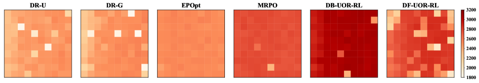
Figure 1: Heat map of $\mathcal{E}_{1}$ in sub-ranges (Half Cheetah). The x-axis and y-axis denote friction and density, respectively. The ranges of these two parameters are chosen as in Table 1, and are evenly divided into 10 sub-ranges.

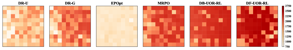
Figure 2: Heat map of $\mathcal{E}_{1}$ in sub-ranges (Hopper). The x-axis and y-axis denote friction and density, respectively. The ranges of these two parameters are chosen as in Table 1, and are evenly divided into 10 sub-ranges.

In the experiments, we let the preference function $W$ take the form as given by Equation (3), which uses a robustness degree $k$ to represent user preference. Thus, we conduct experiments on various UOR metrics, including the average and max-min robustness, by choosing different $k$ in Equation (3), and we use $\mathcal{E}_{k_{0}}$ to denote the UOR metric with $k=k_{0}$.

Considering that the state and action spaces of MuJoCo are high-dimensional and continuous, we choose to use deep neural networks to represent the policies of UOR-RL and the baseline methods, and use PPO [5] to implement the policy updating process.

4.3 Experimental Results and Discussions

We compare UOR-RL with the baseline methods when $k\in\{0,1,21\}$. Specifically, when $k=0$, $W(x)\equiv 1$, and thus $\mathcal{E}_{0}$ is equivalent to the expected return $\mathbb{E}_{p\sim\mathbb{D}}\left[J(\pi,p)\right]$ over the distribution $\mathbb{D}$; when $k=21$, $\mathcal{E}_{21}$ approximates the expected return over the worst 10% trajectories, because more than 90% weight is allocated to them according to the preference function $W$; when $k=1$, $\mathcal{E}_{1}$ represents the UOR metric between $\mathcal{E}_{0}$ and $\mathcal{E}_{21}$.

Table 2 shows the test results under the UOR metric $\mathcal{E}_{1}$. Among all algorithms, DB-UOR-RL performs the best, and it outperforms the four baselines in each environment. Such results indicate that DB-UOR-RL is effective under metric $\mathcal{E}_{1}$. At the same time, although the performance of DF-UOR-RL is not as good as that of DB-UOR-RL, it is better than those of the baselines. This shows that DF-UOR-RL could output competitive policies, even when the distribution of environment parameters is unknown.

Table 3 shows the test result under the average return of all trajectories. In most environments, DR-G achieves the best performance among the baselines under such average-case metric, because it directly takes this average-case metric as its optimization objective. From Table 3, we could observe that the performance of DB-UOR-RL and DF-UOR-RL is close to or better than that of DR-G in most environments. Such observation indicates that UOR-RL can also yield acceptable results, when robustness is not considered.

Table 4 shows the test result under the average return of the worst 10% trajectories. From the table, both DB-UOR-RL and DF-UOR-RL perform no worse than the best baselines in most environments, which shows that UOR-RL also yields sufficiently good performance in terms of the traditional robustness evaluation criteria.

Apart from Tables 2-4, we also visualize the performance of UOR-RL and the baselines in the ranges of environment parameters given by Table 1 by plotting heat maps. Because of space limit, we only show the heat maps of the Half Cheetah and Hopper tasks with $k=1$ in Figures 1 and 2, respectively. In these two figures, a darker color means a better performance. We could observe that both DB-UOR-RL and DF-UOR-RL are darker in color than baselines in most sub-ranges, which supports the superiority of UOR-RL for most environment parameters. Moreover, we place the heat maps of the other four tasks in Appendix C.2.

To show the effect of the robustness degree parameter $k$ on the performance of UOR-RL, we carry out experiments with four robustness degree parameters $k\in\{0,1,5,21\}$ in Half Cheetah under the same environment parameters. The results are shown in Figures 3 and 4. To plot these two figures, we sort the collected trajectories by return into an increasing order, divide the trajectories under such order into 10 equal-size groups, calculate the average return of the trajectories (ART) in each group, and compute the normalized differences between the ARTs that correspond to each consecutive pair of $k$’s in $\{0,1,5,21\}$. We could observe that every curve in these two figures shows a decreasing trend as the group index increases. Such observation indicates that, as $k$ increases, both DB-UOR-RL and DF-UOR-RL pay more attention to the trajectories that perform poorer, and thus the trained policies become more robust.

Additionally, we plot the training curves of the baselines and UOR-RL, and place them in Appendix C.3.

5 Related Work

Robust RL [15, 16, 6] aims to optimize policies under the worst-case environment, traditionally by the zero-sum game formulation [17, 18]. Several recent works focus on finite or linear MDPs, and propose robust RL algorithms with theoretical guarantees [19, 20, 21, 22, 23, 24]. However, real-world applications are usually with continuous state and action spaces, as well as complex non-linear dynamics [25, 26].

A line of deep robust RL works robustify policies against different factors that generate the worst-case environment, such as agents’ observations [27, 28, 29], agents’ actions [8, 30], transition function [31, 32, 33], and reward function [34]. Another line of recent works [25, 11, 13, 35, 36] aim to improve the average performance over all possible environments. Considering only the worst or average case may cause the policy to be overly conservative or aggressive, and limit [27, 28, 29, 8, 30, 31, 32, 33, 34, 25, 11, 13, 35, 36] for boarder applications. Hence, some researches study to use other cases to characterize the robustness of the policy. [37] optimizes the policy performance on $\alpha$-percentile worst-case environments; [38] considers the robustness with a given environment distribution; [39, 40] aim to improve the policy performance on the worst distribution in an environment distribution set.

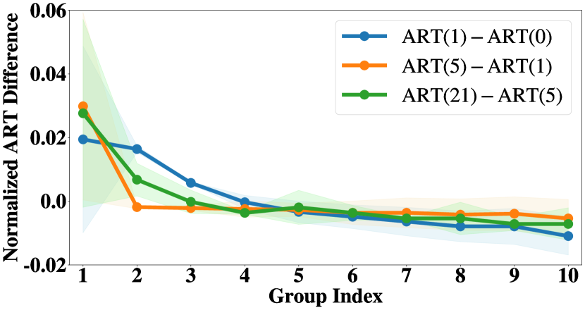
Figure 3: Normalized ART difference for each sorted group (DB-UOR-RL). ART($k_{0}$) denotes the ART with $k=k_{0}$.

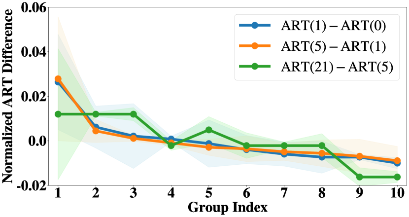
Figure 4: Normalized ART difference for each sorted group (DF-UOR-RL). ART($k_{0}$) denotes the ART with $k=k_{0}$.

Each of [27, 28, 29, 8, 30, 31, 32, 33, 34, 25, 11, 13, 35, 36, 37, 38, 39, 40] optimizes a specific type of robustness, and is only suitable to a specific preference to robustness (e.g. methods focusing on worst case suit the most conservative preference to robustness). However, user preference varies in different scenarios, and an RL method that optimizes a specific type of robustness will be no more suitable when user preference changes. In real applications, it is significant to take user preference into consideration and design a general framework suitable to various types of robustness. Therefore, we design UOR-RL as a general framework, which can be applied to satisfy a variety of preference to robustness. As far as we know, UOR is the first RL framework to take user preference into consideration.

6 Conclusion

In this paper, we propose the UOR metric, which integrates user preference into the measurement of robustness. Aiming at optimizing such metric, we design two UOR-RL training algorithms, which work in the scenarios with or without a priori known environment distribution, respectively. Theoretically, we prove that the output policies of the UOR-RL training algorithms, in the scenarios with accurate, inaccurate or even completely no knowledge of the environment distribution, are all $\epsilon$-suboptimal to the optimal policy. Also, we conduct extensive experiments in 6 MuJoCo tasks, and the results validate that UOR-RL is comparable to the state-of-the-art baselines under traditional metrics and establishes new state-of-the-art performance under the UOR metric.

7 Acknowledgements

This work was supported by NSF China (No. U21A20519, U20A20181, 61902244).

Appendix A Proof of Theorems and Corollary

A.1 Theorem  1

Proof.

We divide the proof into 3 parts.

Continuity of $J(\pi,p)$

Firstly, we want to prove $J(\pi,p)$ is continuous to the environment $p$. In the most of MDPs, the state space and action space $\mathcal{S,A}$ are bounded. Even if $S,A$ are unbounded, we can have function which maps unbounded set into a bounded one. For example, let $\mathcal{S}\in\mathbb{R}^{k}$, we define the function $M:\mathbb{R}^{k}\rightarrow[0,1]^{k}$ that

$$M((x_{1},x_{2},\dots,x_{k})^{T})=(\frac{1}{1+\exp(-x_{1})},\frac{1}{1+\exp(-x_{2})},\dots,\frac{1}{1+\exp(-x_{k})})^{T}.$$ (12)

And if $\mathcal{S,A}$ is not closed, we can also add the boundary into them, that is

$$\mathcal{S}=\mathcal{S}\cup\partial(\mathcal{S}),\mathcal{A}=\mathcal{A}\cup\partial(\mathcal{A}).$$ (13)

As a result, w.l.o.g, we assume $\mathcal{S,A}$ are compact sets.

Furthermore, we can also assume the environment range $\mathcal{P}$ is a compact set. If $\mathcal{P}\in\mathbb{R}^{d}$ is unbounded, we define $B_{r}(0)$ be the closed ball in space $R^{d}$ with center at origin and radius $r$. From the property of distribution $\mathbb{D}$ that

$$1=\int_{\mathcal{P}}\mathbb{D}(p)\mathrm{d}p=\int_{\mathcal{P}\cup B_{\infty}(0)}\mathbb{D}(p)\mathrm{d}p=\lim_{r\rightarrow\infty}\int_{\mathcal{P}\cup B_{r}(0)}\mathbb{D}(p)\mathrm{d}p$$ (14)

Thus for $\forall~{}\varphi,\exists r_{0}$ that

$$\int_{\mathcal{P}\cup B_{r_{0}}(0)}\mathbb{D}(p)\mathrm{d}p>1-\varphi$$ (15)

So we can thake $\mathcal{P}^{\prime}=\mathcal{P}\cup B_{r_{0}}(0)$ to be bounded and use the Theorem 3. As a result, w.l.o.g, we can assume $\mathcal{P}$ is also bounded and compact.

Therefore, the domains of $R$ is $\mathcal{S}^{2}\times\mathcal{A}\times\mathcal{P}\rightarrow R$ is a compact set, so is $T$. From Cantor’s Theorem, we can get $R,T$ is uniformly continue. So we get

$$\forall~{}\epsilon,\exists~{}\delta>0,\forall s\in\mathcal{S},a\in\mathcal{A},p_{1},p_{2}\in\mathcal{P},|p_{1}-p_{2}|<\delta\Rightarrow|R_{p_{1}}(s,a)-R_{p_{2}}(s,a)|<\epsilon$$ (16)

$$\forall~{}\epsilon,\exists~{}\delta>0,\forall s_{1},s_{2}\in\mathcal{S},a\in\mathcal{A},p_{1},p_{2}\in\mathcal{P},|p_{1}-p_{2}|<\delta\Rightarrow|T_{p_{1}}(s_{1},a,s_{2})-T_{p_{2}}(s_{1},a,s_{2})|<\epsilon$$

where for ease of illustration, we use $R_{p}(s,a,s^{\prime}),T_{p}(s,a)$ respectively denote $R_{p}(s,a,s^{\prime},p)$ and $T_{p}(s,a,p)$.

For $\forall$ given $\epsilon$, let set $\Delta_{\epsilon}\subseteq\mathbb{R^{+}}$ satisfies

$$\Delta_{\epsilon}^{R}: =\{\delta~{}|~{}\forall s\in\mathcal{S},a\in\mathcal{A},p_{1},p_{2}\in\mathcal{P},|p_{1}-p_{2}|<\delta\Rightarrow|R_{p_{1}}(s,a)-R_{p_{2}}(s,a)|<\epsilon\}$$ (17)

$$\Delta_{\epsilon}^{T}: =\{\delta~{}|~{}\forall s_{1},s_{2}\in\mathcal{S},a\in\mathcal{A},p_{1},p_{2}\in\mathcal{P},|p_{1}-p_{2}|<\delta\Rightarrow|T_{p_{1}}(s_{1},a,s_{2})-T_{p_{2}}(s_{1},a,s_{2})|<\epsilon\}$$

$\Delta_{\epsilon}^{R}$ has upper bound $d(\mathcal{P})$ (diameter of set $\mathcal{P}$), so it has supremum $\delta_{\epsilon}^{R}$. Here we define a function

$$\delta_{R}(\epsilon)=\delta_{\epsilon}^{R}$$ (18)

Similarly we define the funtion

$$\delta_{T}(\epsilon)=\delta_{\epsilon}^{T}$$ (19)

with $\delta_{\epsilon}^{T}$ as supremum of $\Delta_{\epsilon}^{T}$.

As for $\delta_{R}$, there are several properties

1. Domain of $\delta_{R}$ is $(0,\max R-\min R]$

2. Range of $\delta_{R}\subseteq(0,d(P)]$

3. $\delta_{R}$ is strictly increasing.

Similarly, these properties are the same for $\delta_{T}$.

After that, we discuss $J(\pi,p)$. We define it as

$$J(\pi,p)=\mathbb{E}[\{\sum_{i=0}^{\infty}\gamma^{i}\cdot R_{p}(s_{i},\pi(s_{i}),s_{i+1})\}]$$ (20)

Then we compare the performance of policy $\pi$ under two environments $p_{1}$ and $p_{2}$. We have $s_{0}^{1}=s_{0}^{2}=s_{0}$ and $|p_{1}-p_{2}|<\delta$.

$$J(\pi,p_{1})-J(\pi,p_{2})$$ (21)

$$= \mathbb{E}\left[\sum_{i=0}^{\infty}\gamma^{i}\cdot R_{p_{1}}(s^{1}_{i},\pi(s^{1}_{i},p_{1}),s^{1}_{i+1})\right]-\mathbb{E}\left[\sum_{i=0}^{\infty}\gamma^{i}\cdot R_{p_{2}}(s^{2}_{i},\pi(s^{2}_{i},p_{2}),s^{2}_{i+1})\right]$$

$$= \sum_{i=0}^{\infty}\gamma^{i}\cdot\mathbb{E}\left[R_{p_{1}}(s^{1}_{i},\pi(s^{1}_{i}),s^{1}_{i+1})\right]-\sum_{i=0}^{\infty}\gamma^{i}\cdot\mathbb{E}\left[R_{p_{2}}(s^{2}_{i},\pi(s^{2}_{i}),s^{2}_{i+1})\right]$$

$$= \sum_{i=0}^{\infty}\gamma^{i}\cdot\left[\mathbb{E}\left[R_{p_{1}}(s^{1}_{i},\pi(s^{1}_{i}),s^{1}_{i+1})\right]-\mathbb{E}\left[R_{p_{2}}(s^{2}_{i},\pi(s^{2}_{i}),s^{2}_{i+1})\}\right]\right]$$

We know the distribution of initial state $s_{0}$ is $\mathbb{S}_{0}$. We define that under the environment parameter $p$ and executing policy $\pi$, the state distribution in the $t^{th}$ step is $\mathbb{S}_{t}^{\pi,p}$. And the actions distribution under the state $s$, environment parameter $p$ and executing policy $\pi$ is $\pi^{p}_{s}$. And the transition distribution from state $s$ and action $a$ under parameter $p$ is $T_{p}^{s,a}$.

Then we have

$$\mathbb{E}\left[R_{p_{1}}(s^{1}_{i},\pi(s^{1}_{i}),s^{1}_{i+1})\right]= \int_{\mathcal{S}}\mathbb{S}_{t}^{\pi,p_{1}}(s_{1})\int_{\mathcal{A}}\pi^{p_{1}}_{s}(a)\int_{\mathcal{S}}T_{p_{1}}^{s_{1},a}(s_{2})R_{p_{1}}(s_{1},a,s_{2})\mathrm{d}s_{2}\mathrm{d}a\mathrm{d}s_{1}$$ (22)

$$= R_{p_{1}}(\mathbb{S}_{t}^{\pi,p_{1}},\pi(\mathbb{S}_{t}^{\pi,p_{1}}),T_{p_{1}}(\mathbb{S}_{t}^{\pi,p_{1}},\pi(\mathbb{S}_{t}^{\pi,p_{1}}))).$$

Firstly, we consider the distance of distribution $\mathbb{S}_{t}^{\pi,p_{1}}$ and $\mathbb{S}_{t}^{\pi,p_{2}}$

$$D_{TV}(\mathbb{S}_{t+1}^{\pi,p_{1}},\mathbb{S}_{t+1}^{\pi,p_{2}})$$ (23)

$$= |T_{p_{1}}(\mathbb{S}_{t}^{\pi,p_{1}},\pi(\mathbb{S}_{t}^{\pi,p_{1}}))-T_{p_{2}}(\mathbb{S}_{t}^{\pi,p_{2}},\pi(\mathbb{S}_{t}^{\pi,p_{2}}))|$$

$$= |T_{p_{1}}(\mathbb{S}_{t}^{\pi,p_{1}},\pi(\mathbb{S}_{t}^{\pi,p_{1}}))-T_{p_{1}}(\mathbb{S}_{t}^{\pi,p_{2}},\pi(\mathbb{S}_{t}^{\pi,p_{1}}))+T_{p_{1}}(\mathbb{S}_{t}^{\pi,p_{2}},\pi(\mathbb{S}_{t}^{\pi,p_{1}}))-T_{p_{1}}(\mathbb{S}_{t}^{\pi,p_{2}},\pi(\mathbb{S}_{t}^{\pi,p_{2}}))$$

$$~{}+T_{p_{1}}(\mathbb{S}_{t}^{\pi,p_{2}},\pi(\mathbb{S}_{t}^{\pi,p_{2}}))-T_{p_{2}}(\mathbb{S}_{t}^{\pi,p_{2}},\pi(\mathbb{S}_{t}^{\pi,p_{2}}))|$$

$$\leq L_{T,S}\cdot[D_{TV}(\mathbb{S}_{t}^{\pi,p_{1}},\mathbb{S}_{t}^{\pi,p_{2}})+L_{T,A}L_{\pi}\cdot D_{TV}(\mathbb{S}_{t}^{\pi,p_{1}},\mathbb{S}_{t}^{\pi,p_{2}})]+\delta_{T}^{-1}(\delta)$$

$$= (L_{T,S}+L_{T,A}L_{\pi})\cdot D_{TV}(\mathbb{S}_{t}^{\pi,p_{1}},\mathbb{S}_{t}^{\pi,p_{2}})+\delta_{T}^{-1}(\delta)$$

Then we signal $\Delta^{i}$ and define a new function $dis_{\delta}(x)$.

$$\Delta^{i}:=D_{TV}(\mathbb{S}_{t}^{\pi,p_{1}},\mathbb{S}_{t}^{\pi,p_{2}})~{}~{}~{}~{}~{}~{}~{}~{}~{}dis_{\delta}(x):=(L_{T,S}+L_{T,A}L_{\pi})\cdot x+\delta_{T}^{-1}(\delta).$$ (24)

Then we have $\Delta^{i+1}\leq dis_{\delta}(\Delta^{i})$ Let $dis_{\delta}^{(2)}=dis_{\delta}\circ dis_{\delta}$ and $dis_{\delta}^{(k)}=dis_{\delta}^{(k+1)}\circ dis_{\delta}$
So we can have

$$\Delta^{i}\leq dis_{\delta}(\Delta^{i-1})\leq dis_{\delta}^{(2)}(\Delta^{i-2})\dots\leq dis_{\delta}^{(i)}(\Delta^{0})=dis_{\delta}^{(i)}(|s_{0}^{1}-s_{0}^{2}|)=dis_{\delta}^{(i)}(0).$$ (25)

Let $\alpha=L_{T,S}+L_{T,A}L_{\pi},~{}\beta(\delta)=\delta_{T}^{-1}(\delta)$, then we can simplify the formula that

$$dis_{\delta}^{(i)}(0) =\alpha\cdot dis_{\delta}^{(i-1)}(0)+\beta(\delta)$$ (26)

$$=\alpha^{2}\cdot dis_{\delta}^{(i-2)}(0)+\alpha\cdot\beta(\delta)+\beta(\delta)$$

$$\dots$$

$$=\alpha^{i-1}\cdot dis_{\delta}(0)+\beta(\delta)\cdot\sum_{j=0}^{i-2}\alpha^{j}$$

$$=\left\{\begin{aligned} &\frac{(\alpha^{i}-1)\cdot\beta(\delta)}{\alpha-1}~{}~{}~{}~{}~{}~{}~{}~{}~{}~{}~{}~{}&\alpha>1\\ &i\cdot\alpha\cdot\beta(\delta)~{}~{}~{}~{}~{}~{}~{}~{}&\alpha=1\\ &\frac{(1-\alpha^{i})\cdot\beta(\delta)}{1-\alpha}~{}~{}~{}~{}~{}~{}~{}~{}~{}~{}~{}~{}&\alpha<1\\ \end{aligned}\right.$$

Then consider the distance of reward function $R$

$$\left|R_{p_{1}}(\mathbb{S}_{t}^{\pi,p_{1}},\pi(\mathbb{S}_{t}^{\pi,p_{1}}),T_{p_{1}}(\mathbb{S}_{t}^{\pi,p_{1}},\pi(\mathbb{S}_{t}^{\pi,p_{1}})))-R_{p_{2}}(\mathbb{S}_{t}^{\pi,p_{2}},\pi(\mathbb{S}_{t}^{\pi,p_{2}}),T_{p_{2}}(\mathbb{S}_{t}^{\pi,p_{2}},\pi(\mathbb{S}_{t}^{\pi,p_{2}})))\right|$$ (27)

$$\leq |R_{p_{1}}(\mathbb{S}_{t}^{\pi,p_{1}},\pi(\mathbb{S}_{t}^{\pi,p_{1}}),T_{p_{1}}(\mathbb{S}_{t}^{\pi,p_{1}},\pi(\mathbb{S}_{t}^{\pi,p_{1}})))-R_{p_{1}}(\mathbb{S}_{t}^{\pi,p_{2}},\pi(\mathbb{S}_{t}^{\pi,p_{1}}),T_{p_{1}}(\mathbb{S}_{t}^{\pi,p_{1}},\pi(\mathbb{S}_{t}^{\pi,p_{1}})))|$$

$$+ |R_{p_{1}}(\mathbb{S}_{t}^{\pi,p_{2}},\pi(\mathbb{S}_{t}^{\pi,p_{1}}),T_{p_{1}}(\mathbb{S}_{t}^{\pi,p_{1}},\pi(\mathbb{S}_{t}^{\pi,p_{1}})))-R_{p_{1}}(\mathbb{S}_{t}^{\pi,p_{2}},\pi(\mathbb{S}_{t}^{\pi,p_{2}}),T_{p_{1}}(\mathbb{S}_{t}^{\pi,p_{1}},\pi(\mathbb{S}_{t}^{\pi,p_{1}})))|$$

$$+ |R_{p_{1}}(\mathbb{S}_{t}^{\pi,p_{2}},\pi(\mathbb{S}_{t}^{\pi,p_{2}}),T_{p_{1}}(\mathbb{S}_{t}^{\pi,p_{1}},\pi(\mathbb{S}_{t}^{\pi,p_{1}})))-R_{p_{1}}(\mathbb{S}_{t}^{\pi,p_{2}},\pi(\mathbb{S}_{t}^{\pi,p_{2}}),T_{p_{2}}(\mathbb{S}_{t}^{\pi,p_{2}},\pi(\mathbb{S}_{t}^{\pi,p_{2}})))|$$

$$+ |R_{p_{1}}(\mathbb{S}_{t}^{\pi,p_{2}},\pi(\mathbb{S}_{t}^{\pi,p_{2}}),T_{p_{2}}(\mathbb{S}_{t}^{\pi,p_{2}},\pi(\mathbb{S}_{t}^{\pi,p_{2}})))-R_{p_{2}}(\mathbb{S}_{t}^{\pi,p_{2}},\pi(\mathbb{S}_{t}^{\pi,p_{2}}),T_{p_{2}}(\mathbb{S}_{t}^{\pi,p_{2}},\pi(\mathbb{S}_{t}^{\pi,p_{2}})))|$$

$$\leq L_{R,S}\Delta^{i}+L_{R,A}L_{\pi}(\Delta^{i})+L_{R,S}(\alpha\Delta^{i}+\beta(\delta))+\delta_{R}^{-1}(\delta)$$

Let $\zeta=L_{R,S}+L_{R,A}\cdot L_{\pi}+L_{R,S}\cdot(L_{T,S}+L_{T,A}\cdot L_{\pi})$ and $\eta(\delta)=L_{R,S}\cdot\delta_{T}^{-1}(\delta)+\delta_{R}^{-1}(\delta)$, then we can find a upper bound of the distance of $J(\pi,p_{1})$ and $J(\pi,p_{2})$.

$$J(\pi,p_{1})-J(\pi,p_{2})$$ (28)

$$= \sum_{i=0}^{\infty}\gamma^{i}\cdot\left[\mathbb{E}\left[R_{p_{1}}(s^{1}_{i},\pi(s^{1}_{i}),s^{1}_{i+1})\right]-\mathbb{E}\left[R_{p_{2}}(s^{2}_{i},\pi(s^{2}_{i}),s^{2}_{i+1})\}\right]\right]$$

$$\leq \sum_{i=0}^{\infty}\gamma^{i}(\zeta\cdot\Delta^{i}+\eta(\delta))$$

$$= \frac{\eta(\delta)}{1-\gamma}+\zeta\cdot\sum_{i=0}^{\infty}\gamma^{i}\Delta^{i}$$

Here we need discuss respectively with the relationship with 1 and $\alpha$

$$\sum_{i=0}^{\infty}\gamma^{i}\Delta^{i}=\left\{\begin{aligned} &\sum_{i=0}^{\infty}\gamma^{i}\cdot\frac{(\alpha^{i}-1)\cdot\beta(\delta)}{\alpha-1}\leq\frac{\beta(\delta)}{\alpha-1}\sum_{i=0}^{\infty}(\gamma\cdot\alpha)^{i}\leq\frac{\beta(\delta)}{(\alpha-1)(1-\gamma\cdot\alpha)}~{}~{}~{}~{}&\alpha>1\\ &\sum_{i=0}^{\infty}\gamma^{i}\cdot i\cdot\alpha\cdot\beta(\delta)=\frac{\gamma\cdot\alpha\cdot\beta(\delta)}{(1-\gamma)^{2}}&\alpha=1\\ &\sum_{i=0}^{\infty}\gamma^{i}\cdot\frac{(1-\alpha^{i})\cdot\beta(\delta)}{1-\alpha}\leq\sum_{i=0}^{\infty}\gamma^{i}\cdot\frac{\beta(\delta)}{1-\alpha}=\frac{\beta(\delta)}{(1-\alpha)\cdot(1-\gamma)}&\alpha<1\\ \end{aligned}\right.$$ (29)

Since $\alpha,\zeta,\gamma$ are all fixed constants. We can set

$$\mu_{0} =\max\{\frac{1}{(\alpha-1)(1-\gamma\cdot\alpha)},\frac{\gamma\cdot\alpha}{(1-\gamma)^{2}},\frac{1}{(1-\alpha)\cdot(1-\gamma)}\}$$ (30)

$$\lambda=\frac{1}{1-\gamma}~{}~{}~{}~{}~{}~{}\mu=\mu_{0}\cdot\zeta$$

So we can conclude

$$|J(\pi,p_{1})-J(\pi,p_{2})|\leq\lambda\cdot\eta(\delta)+\mu\cdot\beta(\delta)=:j(\delta)$$ (31)

$\mathcal{E}(\pi)~{}~{}\mathrm{and}~{}~{}\hat{\mathcal{E}}(\pi)$

In this section, we focus on a fixed policy $\pi$, and discuss the value between $\mathcal{E}$ and $\hat{\mathcal{E}}$ executing $\pi$.

As for preference function $W$, if we take normalized one $W^{\prime}$ as the new preference function that

$$W^{\prime}(x)=W(x)/\mathcal{W}~{}~{}with~{}~{}~{}\mathcal{W}=\int_{0}^{1}W(x)\mathrm{d}x$$ (32)

The optimal policy keeps the same. That is, we can normalize the preference function will the actually influence the UOR-PMDP. As a result, w.l.o.g, we can assume

$$\int_{0}^{1}W(x)\mathrm{d}x=1.$$ (33)

From the calculation of $\hat{\mathcal{E}}(\pi)$, we can define a new function $H^{\prime}_{\pi}$ as a step function, assume the order is $\alpha_{1}$ to $\alpha_{n}$

$$M_{i}= \sum_{k=1}^{i}m_{\alpha_{i}}~{}~{}~{}~{}(M_{0}=0)$$ (34)

$$H^{\prime}_{\pi}(x)=J(\pi,p_{\alpha_{i}}){}{}{}{}{} with~{}~{}~{}M_{i-1}\leq x<M_{i}$$

From the definition of $\mathcal{E}$, we know

$$\mathcal{E}(\pi)=\int_{\mathcal{P}}\mathbb{D}(p)\cdot J(\pi,p)\cdot W(h(\pi,p))\mathrm{d}p.$$ (35)

We define another function $H$ that

$$H(x):=\int_{\mathcal{P}}\mathbb{D}(p)\cdot\mathds{1}\left[J(\pi,p)\leq x\right]\mathrm{d}p$$ (36)

From the definition we get easily get

$$H(J(\pi,p))=h(\pi,p).$$ (37)

For the function $H$, we find $H$ is monotonic increasing. We signal $H^{-1}$ as the inverse function of $H$. It’s important to mention that since $H$ may be not strictly increasing, the true inverse function may not exists, but we can let the lower bound one as the value of the $H^{-1}$, so we assume the inverse function existing.

After that we can have

$$\mathcal{E}(\pi) =\int_{\mathcal{P}}\mathbb{D}(p)\cdot J(\pi,p)\cdot W(h(\pi,p))\mathrm{d}p$$ (38)

$$=\int_{\mathcal{P}}(H_{\pi}^{-1}(h(\pi,p))\cdot W(h(\pi,p))(\mathbb{D}(p)\mathrm{d}p)$$

$$\overset{x=h(\pi,p)}{=}\int_{0}^{1}H_{\pi}^{-1}(x)\cdot W(x)\mathrm{d}x$$

Also we have

$$\hat{\mathcal{E}}(\pi)=\int_{0}^{1}H^{\prime}_{\pi}(x)\cdot W(x)\mathrm{d}x.$$ (39)

As a result

$$|\mathcal{E}(\pi)-\hat{\mathcal{E}}(\pi)|$$ (40)

$$= |\int_{0}^{1}(H_{\pi}^{-1}(x)-H^{\prime}_{\pi}(x))\cdot W(x)|$$

$$= |\sum_{i=0}^{n}\int_{M_{i}}^{M_{i+1}}(H_{\pi}^{-1}(x)-H^{\prime}_{\pi}(x))\cdot W(x)|$$

$$\leq \sum_{i=0}^{n}\int_{M_{i}}^{M_{i+1}}|H_{\pi}^{-1}(x)-H^{\prime}_{\pi}(x)|\cdot W(x)$$

We from two direction to bound $H_{\pi}^{-1}-H^{\prime}_{\pi}$

1. $H^{\prime}_{\pi}(x)\geq H_{\pi}^{-1}(x)-j(\delta):$

   $$Let~{}~{}M_{i}\leq x<M_{i+1}\Rightarrow\forall j<i,J(\pi,p_{l^{j}})\leq H^{\prime}_{\pi}(x)$$ (41)

   $$From~{}~{}\forall k,d(\mathcal{P}_{k})\leq\delta$$

   $$\Rightarrow \forall y\in\mathcal{P}_{l^{j}},|J(\pi,p_{l^{j}})-J(\pi,y)|<j(\delta)$$

   $$\Rightarrow J(\pi,y)\leq J(\pi,p_{l^{j}})+j(\delta)\leq H^{\prime}_{\pi}(x)+j(\delta)$$

   $$Let~{}~{}\mathbb{U}_{i}=\bigcup_{j=0}^{i}\mathcal{P}_{\alpha_{j}}$$

   $$\Rightarrow \forall y\in\mathbb{U}_{i},J(\pi,y)<H^{\prime}_{\pi}(x)+j(\delta)$$

   $$We~{}know,~{}\int_{\mathbb{U}_{i}}\mathbb{D}(p)\mathrm{d}p=M_{i+1}$$

   $$\Rightarrow \int_{\mathcal{P}}\mathds{1}[J(\pi,p)<H^{\prime}_{\pi}(x)+j(\delta)]\cdot\mathbb{D}(p)\mathrm{d}p\geq M_{i+1}~{}~{}~{}~{}~{}~{}~{}~{}~{}~{}~{}~{}~{}~{}~{}~{}~{}~{}~{}~{}~{}~{}~{}~{}~{}~{}~{}~{}~{}~{}~{}~{}~{}$$

   $$\Rightarrow H_{\pi}^{-1}(x)\leq H_{\pi}^{-1}(M_{i+1})\leq H^{\prime}_{\pi}(x)+j(\delta)$$

   $$\Rightarrow H^{\prime}_{\pi}(x)\geq H_{\pi}^{-1}(x)-j(\delta)$$

2. $H^{\prime}_{\pi}(x)\leq H_{\pi}^{-1}(x)+j(\delta)$:

   $$Let~{}~{}M_{i}\leq x<M_{i+1}\Rightarrow\forall j>i,J(\pi,p_{l^{j}})\geq H^{\prime}_{\pi}(x)$$ (42)

   $$From~{}~{}\forall k,d(\mathcal{P}_{k})\leq\delta$$

   $$\Rightarrow \forall y\in\mathcal{P}_{l^{j}},|J(\pi,p_{l^{j}})-J(\pi,y)|<j(\delta)$$

   $$\Rightarrow J(\pi,y)\geq J(\pi,p_{l^{j}})-j(\delta)\geq H^{\prime}_{\pi}(x)-j(\delta)$$

   $$Let~{}~{}\mathbb{V}_{i}=\bigcup_{j=i}^{n}\mathcal{P}_{\alpha^{j}}$$

   $$\Rightarrow \forall y\in\mathbb{V}_{i},J(\pi,y)\geq H^{\prime}_{\pi}(x)-j(\delta)$$

   $$We~{}know,~{}\int_{\mathbb{V}_{i}}\mathbb{D}(p)\mathrm{d}p=1-M_{i}$$

   $$\Rightarrow \int_{\mathcal{P}}\mathds{1}[J(\pi,p)\geq H^{\prime}_{\pi}(x)-j(\delta)]\cdot\mathbb{D}(p)\mathrm{d}p\geq 1-M_{i}~{}~{}~{}~{}~{}~{}~{}~{}~{}~{}~{}~{}~{}~{}~{}~{}~{}~{}~{}~{}~{}~{}~{}~{}~{}~{}~{}~{}~{}~{}~{}~{}~{}$$

   $$A nd\int_{\mathcal{P}}\mathds{1}[J(\pi,p)\geq H^{\prime}_{\pi}(x)-j(\delta)]\cdot\mathbb{D}(p)\mathrm{d}p+\int_{\mathcal{P}}\mathds{1}[J(\pi,p)\leq H^{\prime}_{\pi}(x)-j(\delta)]\cdot\mathbb{D}(p)\mathrm{d}p$$

   $$= \int_{\mathcal{P}}\mathds{1}\cdot\mathbb{D}(p)\mathrm{d}p-\int_{\mathcal{P}}\mathds{1}[J(\pi,p)=H^{\prime}_{\pi}(x)-j(\delta)]\cdot\mathbb{D}(p)\mathrm{d}p=1-0=1$$

   $$\Rightarrow \int_{\mathcal{P}}\mathds{1}[J(\pi,p)\leq H^{\prime}_{\pi}(x)-j(\delta)]\cdot\mathbb{D}(p)\mathrm{d}p\leq M_{i}$$

   $$\Rightarrow H_{\pi}^{-1}(x)\geq H_{\pi}^{-1}(M_{i})\geq H^{\prime}_{\pi}(x)+j(\delta)$$

   $$\Rightarrow H^{\prime}_{\pi}(x)\leq H_{\pi}^{-1}(x)+j(\delta)$$

As a result, we can conclude $|H^{\prime}_{\pi}(x)-H_{\pi}^{-1}(x)|\leq j(\delta)$, Then

$$|\mathcal{E}(\pi)-\hat{\mathcal{E}}(\pi)|$$ (43)

$$\leq \sum_{i=0}^{n}\int_{M_{i}}^{M_{i+1}}|H_{\pi}^{-1}(x)-H^{\prime}_{\pi}(x)|\cdot W(x)\mathrm{d}x$$

$$\leq \sum_{i=0}^{n}\int_{M_{i}}^{M_{i+1}}j(\delta)\cdot W(x)\mathrm{d}x$$

$$= j(\delta)\cdot\sum_{i=0}^{n}\int_{M_{i}}^{M_{i+1}}W(x)\mathrm{d}x$$

$$= j(\delta)\cdot\int_{0}^{1}W(x)\mathrm{d}x$$

$$= j(\delta)$$

with

$\hat{\pi}$, $\pi^{*}$

We define these two optimal policies that

$$\pi^{*}=\operatorname*{arg\,max}_{\pi}\mathcal{E}(\pi)$$ (44)

$$\hat{\pi}^{\ast}=\operatorname*{arg\,max}_{\pi}\hat{\mathcal{E}}(\pi)$$

Consider the function $j(\delta)=\eta(\delta)+\mu\cdot\beta(\delta)$ that

$$\beta(\delta) =L_{T,A}L_{\pi}\delta+\delta_{T}^{-1}(\delta)$$ (45)

$$\eta(\delta) =L_{R,S}\cdot\delta_{T}^{-1}(\delta)+\delta_{R}^{-1}(\delta).$$

$\delta_{T}$ and $\delta_{R}$ is a strictly increasing function, and $\delta_{T}(0)=\delta_{R}(0)=0$. So we know $\beta(\delta)$ ,$\eta(\delta)$ and $j(\delta)$ are all strictly increasing and $\beta(0)=\eta(0)=j(0)=0$. As a result, $j^{-1}$ exists and is strictly increasing with $j^{-1}(0)=0$.

Then for $\forall\epsilon=2\epsilon_{0}$, let $\delta_{0}=j^{-1}(\epsilon_{0}/2)$. As long as we have block diameter upper bound is $\delta_{0}$ then we can get

$$\forall policy~{}~{}\pi,|\mathcal{E}(\pi)-\hat{\mathcal{E}}(\pi)|\leq j(\delta_{0})=j(j^{-1}(\epsilon/2))=\epsilon/2.$$ (46)

And we know the Policy_Update function can output $\epsilon_{0}-suboptimal$ policy $\hat{\pi}$, that is

$$\hat{\mathcal{E}}(\hat{\pi})\geq\hat{\mathcal{E}}(\hat{\pi}^{\ast})-\epsilon_{0}$$ (47)

Then we can conclude the proof above that

$$\mathcal{E}(\hat{\pi})\geq\hat{\mathcal{E}}(\hat{\pi})-\epsilon_{0}/2\geq\hat{\mathcal{E}}(\hat{\pi}^{\ast})-3\epsilon_{0}/2\geq\hat{\mathcal{E}}(\pi^{\ast})-3\epsilon_{0}/2\geq\mathcal{E}(\pi^{\ast})-2\epsilon_{0}=\mathcal{E}(\pi^{\ast})-\epsilon$$ (48)

Then we prove this theorem. ∎

A.2 Theorem  2

Proof.

Since the we strengthen the Assumption 1 and get the Lipschitz continuity one, Assumption 4, we can modify the proof of Theorem 1 that

$$\delta_{T}(\delta)= L_{T,p}\cdot\delta$$ (49)

$$\delta_{R}(\delta)= L_{R,p}\cdot\delta$$

As a result, we can get accurate value of $\beta$ and $\eta$ that

$$\beta(\delta) =\frac{\delta}{L_{T,p}}$$ (50)

$$\eta(\delta) =\frac{L_{R,S}\cdot\delta}{L_{T,p}}+\frac{\delta}{L_{R,p}}.$$

So we can have the $j(\delta)$ that

$$j(\delta) =\lambda\eta(\delta)+\mu\beta(\delta)$$ (51)

$$=\frac{\frac{L_{R,S}\cdot\delta}{L_{T,p}}+\frac{\delta}{L_{R,p}}}{1-\gamma}+[L_{R,S}+L_{R,A}\cdot L_{\pi}+L_{R,S}\cdot(L_{T,S}+L_{T,A}\cdot L_{\pi})]\mu_{0}\cdot\frac{\delta}{L_{T,p}}$$

$$=[\frac{L_{R,p}L_{R,S}+L_{T,p}}{L_{T,p}L_{R,p}(1-\gamma)}+\frac{(L_{R,S}+L_{R,A}L_{\pi}+L_{R,S}(L_{T,S}+L_{T,A}L_{\pi}))\mu_{0}}{L_{T,p}}]\delta$$

$$=:\frac{\delta}{\upsilon}$$

with

$$\mu_{0}=\max\{\frac{1}{(\alpha-1)(1-\gamma\cdot\alpha)},\frac{\gamma\cdot\alpha}{(1-\gamma)^{2}},\frac{1}{(1-\alpha)\cdot(1-\gamma)}\}$$ (52)

Then we can have $j^{-1}(\epsilon)=\upsilon\epsilon=O(\epsilon)$. ∎

A.3 Theorem  3

Proof.

First, we define two function

$$H_{\pi}(x)= \int_{\mathcal{P}}\mathds{1}[J(\pi,p)\leq x]\cdot\mathbb{D}(p)\mathrm{d}p$$ (53)

$$H_{\pi,e}(x)= \int_{\mathcal{P}}\mathds{1}[J(\pi,p)\leq x]\cdot\mathbb{D}^{e}(p)\mathrm{d}p$$

So from that, we know

$$\mathcal{E}(\pi)= \int_{0}^{1}H^{-1}_{\pi}(x)\cdot W(x)\mathrm{d}x$$ (54)

$$\mathcal{E}^{e}(\pi)= \int_{0}^{1}H^{-1}_{\pi,\mathbb{D}^{e}}(x)\cdot W(x)\mathrm{d}x$$

Before that, there is a property

Lemma 5.

$$\exists J_{0},\forall~{}policy~{}\pi,\forall~{}0\leq x\leq 1,~{}\forall\mathbb{D},~{}|H^{-1}_{\pi}(x)|\leq J_{0}$$ (55)

Proof.

For $\forall~{}policy~{}\pi,\forall~{}0\leq x\leq 1,~{}\forall\mathbb{D}$, there exists $p_{1},p_{2}\in\mathcal{P}$,

$$J(\pi,p_{1})\leq H^{-1}_{\pi}(x)\leq J(\pi,p_{2}).$$ (56)

Exactly, we can get the $p_{1}=\operatorname*{arg\,min}_{p\in\mathcal{P}}J(\pi,p),p_{2}=\operatorname*{arg\,max}_{p\in\mathcal{P}}J(\pi,p)$

After that, from assumption 4,5, $R$ function is continue to $\mathcal{P}$, Lipschitz to $S$ and $A$, so $R$ is continue in its domain $\mathbb{S}^{2}\times\mathbb{A}\times\mathcal{P}$.

Besides, from assumption 1,2,6, we get the domain of $R$ is a compact set, with the continuity of $R$, we know range of $R$ is a compact set, so its bounded. We can assume

$$|R_{p}(s,a,s^{\prime})|\leq R_{0}$$ (57)

Then we can get

$$\forall p,\pi,|J(\pi,p)| =|\mathbb{E}[\{\sum_{i=0}^{\infty}\gamma^{i}\cdot R_{p_{1}}(s_{i},\pi(s_{i}),s_{i+1})\}]|$$ (58)

$$\leq\mathbb{E}[\sum_{i=0}^{\infty}\gamma^{i}*R_{0}]$$

$$=\frac{R_{0}}{1-\gamma}$$

Let $J_{0}=\frac{R_{0}}{1-\gamma}$, we have

$$-\frac{R_{0}}{1-\gamma}\leq J(\pi,p_{1}) \leq H^{-1}_{\pi}(x)\leq J(\pi,p_{2})\leq\frac{R_{0}}{1-\gamma}$$ (59)

$$\Longrightarrow |H^{-1}_{\pi}(x)|\leq\frac{R_{0}}{1-\gamma}$$

∎

Lemma 6.

$\forall$ given $\epsilon>0,policy~{}\pi$, $\exists~{}\kappa=O(\epsilon)$, as long as $D_{TV}(\mathbb{D},\mathbb{D}^{e})\leq\kappa$, then we can promise

$$|\mathcal{E}(\pi)-\mathcal{E}^{e}(\pi)|\leq\epsilon$$ (60)

Proof.

We divide $\mathcal{E}(\pi)$ into 2 parts.

$$\mathcal{E}(\pi) =\int_{0}^{1}H_{\pi}^{-1}(x)\cdot W(x)\mathrm{d}x$$ (61)

$$=\int_{0}^{0^{+}}H_{\pi}^{-1}(x)\cdot W(x)\mathrm{d}x+\int_{0^{+}}^{1}H_{\pi}^{-1}(x)\cdot W(x)\mathrm{d}x$$

$$: =\mathcal{E}_{1}(\pi)+\mathcal{E}_{2}(\pi)$$

Then we can easily get

$$|\mathcal{E}(\pi)-\mathcal{E}^{e}(\pi)|\leq|\mathcal{E}_{1}(\pi)-\mathcal{E}^{e}_{1}(\pi)|+|\mathcal{E}_{2}(\pi)-\mathcal{E}^{e}_{2}(\pi)|$$ (62)

Part 1:$\mathcal{E}_{1}(\pi)$

From the definition, we have

$$\mathcal{E}_{1}(\pi)=\int_{0}^{0^{+}}W(x)\mathrm{d}x\cdot\lim_{x\to 0^{+}}H_{\pi}^{-1}(x)$$ (63)

Let $A=\int_{0}^{0^{+}}W(x)\mathrm{d}x$, then we get

$$|\mathcal{E}_{1}(\pi)-\mathcal{E}^{e}_{1}(\pi)|=A\cdot\lim_{x\to 0^{+}}|H_{\pi}^{-1}(x)-H_{\pi,e}^{-1}(x)|$$ (64)

Since the environment distribution will not change abruptly, we can mildly assume the distribution function is continuous, that is, $\mathbb{D}(p)$ is continuous to $p$. Then as $\mathcal{P}$ is a compact set, so $\mathbb{D}$ is uniformly continuous. Let $p_{0}$ be the worst-case environment parameter for distribution $\mathbb{D}$ that $h(\pi,p_{0})=0$. Then, w.l.o.g, let $\mathbb{D}(p_{0})=D>0$. Then since the uniform continuity of $\mathbb{D}$, for $\frac{D}{2}$, $\exists~{}\delta_{1}$, for $\forall~{}p_{1}\in\mathcal{P}$ and $|p_{0}-p_{1}|<\delta_{1}$, then $|\mathbb{D}(p_{0})-\mathbb{D}(p_{1})|<\frac{D}{2}$. As a result, we have

$$\forall~{}p\in B_{\delta_{1}}(p_{0}),\frac{D}{2}<\mathbb{D}(p)<\frac{3D}{2}$$ (65)

$$\Rightarrow \int_{B_{\delta_{1}}(p_{0})}\mathbb{D}(p)\mathrm{d}p>c\cdot\delta_{1}^{d}\cdot\frac{D}{2},$$

where $c\delta_{1}^{d}$ is the volume of the ball $B_{\delta_{1}}(p_{0})$ and $c$ depends on the dimension of environment parameter space.

According to Theorem 2, for $\frac{\epsilon}{3A},\exists~{}\delta_{0}=\frac{\upsilon\epsilon}{3A}$. Since the definition of $O()$ and that as $\epsilon\rightarrow 0,\delta_{0}\rightarrow 0$, we can let $\delta_{0}<\delta_{1}$. Then we choose $\kappa_{1}=c\cdot\delta_{0}^{d}\cdot\frac{D}{2}=O(\delta_{0}^{d})=O(\epsilon^{d})$, if $D_{TV}(\mathbb{D},\mathbb{D}^{e})<\kappa_{0}$, then

$$\int_{B_{\delta_{0}}(p_{0})}\mathbb{D}^{e}(p)\mathrm{d}p>0.$$ (66)

Therefore, $\exists~{}p^{\prime}\in B_{\delta_{0}}$ that $\mathbb{D}^{e}(p^{\prime})>0$, then

$$\lim_{x\rightarrow 0^{+}}H^{-1}_{\pi,e}(x)\geq\lim_{x\rightarrow 0^{+}}H^{-1}_{\pi}(x)-\epsilon.$$ (67)

Similarly, when consider the worst case in $\mathbb{D}^{e}$, we can get

$$\lim_{x\rightarrow 0^{+}}H^{-1}_{\pi}(x)\geq\lim_{x\rightarrow 0^{+}}H^{-1}_{\pi,e}(x)-\epsilon.$$ (68)

As a result, as long as $D_{TV}(\mathbb{D},\mathbb{D}^{e})\leq\kappa_{1}$, we can guarantee

$$|\mathcal{E}_{1}(\pi)-\mathcal{E}^{e}_{1}(\pi)|=A\cdot\lim_{x\to 0^{+}}|H_{\pi}^{-1}(x)-H_{\pi,e}^{-1}(x)|<A\cdot\frac{\epsilon}{3A}=\frac{\epsilon}{3}$$ (69)

Part 2:$\mathcal{E}_{2}(\pi)$

From

$$0=\int_{0^{+}}^{0^{+}}W(x)\mathrm{d}x=\lim_{x\rightarrow 0^{+}}\int_{0^{+}}^{x}W(x)\mathrm{d}x$$ (70)

we know for given $\epsilon$

$$\exists\sigma>0,\mathrm{s.t.}\int_{0^{+}}^{\sigma}W(x)\mathrm{d}x\leq\frac{\epsilon}{6J_{0}}$$ (71)

From the limitation of the $W$, we know $W$ is monotonic decreasing, so

$$\forall\sigma\leq x\leq 1,W(x)\leq W(\sigma)$$ (72)

Then we extend the $W$ function to $W_{1}$ that

$$W_{1}(x)=\left\{\begin{aligned} W(x)~{}~{}~{}~{}~{}x\geq\sigma\\ W(\sigma)~{}~{}~{}~{}~{}x\leq\sigma\end{aligned}\right.$$ (73)

So we can change the $W$ into $W_{1}$ that for $\forall\mathbb{D},\pi$, we have

$$\mathcal{E}_{2}(\pi)-\int_{0}^{1}H_{\pi}^{-1}(x)\cdot W_{1}(x)\mathrm{d}x$$ (74)

$$= \mathcal{E}_{2}(\pi)-\int_{0^{+}}^{1}H_{\pi}^{-1}(x)\cdot W_{1}(x)\mathrm{d}x$$

$$= \int_{0^{+}}^{1}H_{\pi}^{-1}(x)\cdot[W(x)-W_{1}(x)]\mathrm{d}x$$

$$= \int_{0^{+}}^{\sigma}H_{\pi}^{-1}(x)\cdot[W(x)-W_{1}(x)]\mathrm{d}x$$

$$\leq J_{0}\cdot\int_{0^{+}}^{\sigma}[W(x)-W_{1}(x)]\mathrm{d}x$$

$$\leq J_{0}\cdot\int_{0^{+}}^{\sigma}W(x)\mathrm{d}x=\frac{\epsilon}{6}$$

Then we can change the $E_{2}$ into another form

$$|\mathcal{E}_{2}(\pi)-\mathcal{E}^{e}_{2}(\pi)|$$ (75)

$$\leq |\mathcal{E}_{2}(\pi)-\int_{0}^{1}H_{\pi}^{-1}(x)\cdot W_{1}(x)\mathrm{d}x-\mathcal{E}^{e}_{2}(\pi)+\int_{0}^{1}H_{\pi,e}^{-1}(x)\cdot W_{1}(x)\mathrm{d}x|$$

$$+ |\int_{0}^{1}H_{\pi}^{-1}(x)\cdot W_{1}(x)\mathrm{d}x-\int_{0}^{1}H_{\pi,e}^{-1}(x)\cdot W_{1}(x)\mathrm{d}x|$$

$$\leq |\mathcal{E}_{2}(\pi)-\int_{0}^{1}H_{\pi}^{-1}(x)\cdot W_{1}(x)\mathrm{d}x|+|\mathcal{E}^{e}_{2}(\pi)-\int_{0}^{1}H_{\pi,e}^{-1}(x)\cdot W_{1}(x)\mathrm{d}x|$$

$$+ |\int_{0}^{1}H_{\pi}^{-1}(x)\cdot W_{1}(x)\mathrm{d}x-\int_{0}^{1}H_{\pi,e}^{-1}(x)\cdot W_{1}(x)\mathrm{d}x|$$

$$\leq \frac{\epsilon}{6}+\frac{\epsilon}{6}+|\int_{0}^{1}H_{\pi}^{-1}(x)\cdot W_{1}(x)\mathrm{d}x-\int_{0}^{1}H_{\pi,e}^{-1}(x)\cdot W_{1}(x)\mathrm{d}x|$$

$$= \frac{\epsilon}{3}+|\int_{0}^{1}H_{\pi}^{-1}(x)\cdot W_{1}(x)\mathrm{d}x-\int_{0}^{1}H_{\pi,e}^{-1}(x)\cdot W_{1}(x)\mathrm{d}x|$$

And we also have

$$= |\int_{\sigma}^{1}H_{\pi}^{-1}(x)\cdot W_{1}(x)\mathrm{d}x-\int_{\sigma}^{1}H_{\pi,e}^{-1}(x)\cdot W_{1}(x)\mathrm{d}x|$$ (76)

$$= |\int_{\mathcal{P}}J(\pi,p)\cdot\mathbb{D}(p)\cdot W_{1}(h(\pi,p))\mathrm{d}p-\int_{\mathcal{P}}J(\pi,p)\cdot\mathbb{D}^{e}(p)\cdot W_{1}(h^{e}(\pi,p))\mathrm{d}p|$$

$$\leq \int_{\mathcal{P}}J(\pi,p)\cdot|\mathbb{D}(p)\cdot W_{1}(h(\pi,p))-\mathbb{D}^{e}(p)\cdot W_{1}(h^{e}(\pi,p))|\mathrm{d}p$$

$$\leq J_{0}\cdot\int_{\mathcal{P}}|\mathbb{D}(p)\cdot W_{1}(h(\pi,p))-\mathbb{D}^{e}(p)\cdot W_{1}(h^{e}(\pi,p))|\mathrm{d}p$$

$$\leq J_{0}\cdot[\int_{\mathcal{P}}\mathbb{D}(p)\cdot|W_{1}(h(\pi,p))-W_{1}(h^{e}(\pi,p))|+|\mathbb{D}(p)-\mathbb{D}^{e}(p)|\cdot W_{1}(h^{e}(\pi,p))\mathrm{d}p]$$

we consider that $W_{1}$ is Lipschitz continuous in $[\sigma,1]$, which means

$$\forall~{}\frac{\epsilon}{6J_{0}},\exists\kappa_{2}=O(\epsilon)>0,|x_{1}-x_{2}|<\kappa_{2}\Rightarrow|W_{1}(x_{1})-W_{1}(x_{2})|\leq\frac{\epsilon}{6J_{0}}$$ (77)

So for the distance of $h$, we can get

$$|h(\pi,p)-h^{e}(\pi,p)|$$ (78)

$$= |\int_{\mathcal{P}}\mathbb{D}(p)\cdot\mathds{1}[J(\pi,p)\geq J(\pi,p^{\prime})]\mathrm{d}p^{\prime}-\int_{\mathcal{P}}\mathbb{D}^{e}(p)\cdot\mathds{1}[J(\pi,p)\geq J(\pi,p^{\prime})]\mathrm{d}p^{\prime}|$$

$$\leq \int_{\mathcal{P}}|\mathbb{D}(p)-\mathbb{D}^{e}(p)|\cdot\mathds{1}[J(\pi,p)\geq J(\pi,p^{\prime})]\mathrm{d}p^{\prime}$$

$$\leq \int_{\mathcal{P}}|\mathbb{D}(p)-\mathbb{D}^{e}(p)|\cdot\mathrm{d}p^{\prime}=D_{TV}(\mathbb{D},\mathbb{D}^{e})$$

If we guarantee $D_{TV}(\mathbb{D},\mathbb{D}^{e})<\kappa_{2}$, then we have

$$|W_{1}(h(\pi,p))-W_{1}(h^{e}(\pi,p))|\leq\frac{\epsilon}{6J_{0}}$$ (79)

Let $\kappa_{3}=\frac{\epsilon}{6\cdot J_{0}\cdot W(\sigma)}=O(\epsilon)$, then if guarantee $D_{TV}(\mathbb{D},\mathbb{D}^{e})\leq\kappa_{3}$, then we have

$$= |\int_{\sigma}^{1}H_{\pi}^{-1}(x)\cdot W_{1}(x)\mathrm{d}x-\int_{\sigma}^{1}H_{\pi,e}^{-1}(x)\cdot W_{1}(x)\mathrm{d}x|$$ (80)

$$\leq J_{0}\cdot[\int_{\mathcal{P}}\mathbb{D}(p)\cdot|W_{1}(h(\pi,p))-W_{1}(h^{e}(\pi,p))|+|\mathbb{D}(p)-\mathbb{D}^{e}(p)|\cdot W_{1}(h^{e}(\pi,p))\mathrm{d}p]$$

$$\leq J_{0}\cdot\frac{\epsilon}{6J_{0}}\cdot\int_{\mathcal{P}}\mathbb{D}(p)\mathrm{d}p+J_{0}\cdot W(\sigma)\cdot\int_{\mathcal{P}}|\mathbb{D}(p)-\mathbb{D}^{e}(p)|\mathrm{d}p$$

$$\leq J_{0}\cdot\frac{\epsilon}{6J_{0}}+J_{0}\cdot W(\sigma)\cdot\kappa_{3}$$

$$= J_{0}\cdot\frac{\epsilon}{6J_{0}}+J_{0}\cdot W(\sigma)\cdot\frac{\epsilon}{6\cdot J_{0}\cdot W(\sigma)}$$

$$= \frac{\epsilon}{6}+\frac{\epsilon}{6}=\frac{\epsilon}{3}$$

Conclusion

Let $\kappa=\min\{\kappa_{1},\kappa_{2},\kappa_{3}\}=\min\{O(\epsilon^{d}),O(\epsilon),O(\epsilon)\}=O(\epsilon^{d})$, and we let $D_{TV}(\mathbb{D},\mathbb{D}^{e})<\kappa$, so we can get

$$|\mathcal{E}(\pi)-\mathcal{E}^{e}(\pi)|$$ (81)

$$\leq |\mathcal{E}_{1}(\pi)-\mathcal{E}^{e}_{1}(\pi)|+|\mathcal{E}_{2}(\pi)-\mathcal{E}^{e}_{2}(\pi)|$$

$$\leq \frac{\epsilon}{3}+\frac{\epsilon}{3}+|\int_{0}^{1}H_{\pi}^{-1}(x)\cdot W_{1}(x)\mathrm{d}x-\int_{0}^{1}H_{\pi,e}^{-1}(x)\cdot W_{1}(x)\mathrm{d}x|$$

$$\leq \frac{\epsilon}{3}+\frac{\epsilon}{3}+\frac{\epsilon}{3}=\epsilon$$

∎ Back to Theorem 3, for $\forall~{}\epsilon$, let $\epsilon_{0}=\epsilon/2$, and use Lemma 60 with $\epsilon_{0}$, we can get

$$\mathcal{E}(\pi^{e}) \geq E(\pi^{e},f,\mathbb{D}^{e})-\epsilon_{0}$$ (82)

$$\geq\mathcal{E}^{e}(\pi^{e})$$

$$\geq\mathcal{E}(\pi)-\epsilon_{0}-\epsilon_{0}$$

$$=\mathcal{E}(\pi)-\epsilon$$

∎

A.4 Corollary 10

Proof.

Since the Update_Policy learn an $\epsilon$-suboptimal policy, we have

$$\mathcal{E}^{e}(\hat{\pi}^{e})\geq\mathcal{E}^{e}(\pi^{e})-\epsilon.$$ (83)

And according to Lemma 60 with $\epsilon$, we get

$$\mathcal{E}(\hat{\pi}^{e})\geq \mathcal{E}^{e}(\hat{\pi}^{e})-\epsilon$$ (84)

$$\geq \mathcal{E}^{e}(\pi^{e})-2\epsilon$$

$$\geq \mathcal{E}^{e}(\pi^{\ast})-2\epsilon$$

$$\geq \mathcal{E}(\pi^{\ast})-3\epsilon$$

$$= \mathcal{E}(\pi^{\ast})-\epsilon_{1}$$

∎

A.5 Theorem  4

In Algorithm 2, for each trajectory $\xi_{j,k}$, we regard its environment parameter $p_{j,k}$ as a random variable. For $\forall~{}j,k$, the environment parameter $p_{j,k}$ is a random variable. These environment parameter all follow a priori distribution $\mathbb{D}$ but is not independent to each other, for it is mild to assume the environment will not change abruptly. In Algorithm 2, we sample these trajetories one by one. For ease of illustration, we mark the first trajectories in each cluster $\xi_{j,0}$ as the $\xi_{j}$ to represent the whole cluster, and $p_{j,0}$ as $p_{j}$.

Then we define the posterior distribution $\mathbb{D}_{x}^{y}$, which means the probability distribution of random variable $p_{y}$ after observing the $p_{x}$. Then we propose the following assumption

Assumption 5.

The environment parameter change continuously between trajectories that the distance between to consecutive environment parameter is not too larger that

$$\forall~{}j,k,|p_{j,k}-p_{j.k+1}|<\frac{\epsilon}{2\upsilon m_{1}},$$ (85)

where $\upsilon$ is defined in Theorem 2 and $m_{1}$ is the cluster size.

The posterior distribution probability of $\mathbb{D}_{x}^{y}$ will converge to its stable distribution $\mathbb{D}$ with the rate that

$$\sum_{y=x}^{\infty}D_{TV}(\mathbb{D},\mathbb{D}_{x}^{y})<\infty,$$ (86)

which means the posterior converge rate is faster than harmonic series.

Then we prove the Theorem 4.

Proof.

Lemma 7.

For given $\epsilon_{0}$ and confidence $\rho_{0}$, let

$$n_{2}=\frac{-8\cdot R_{max}^{2}\cdot\ln\rho_{0}}{(1-\gamma)^{2}\cdot\epsilon_{0}^{2}}=O(-\frac{\ln\rho_{0}}{\epsilon_{0}^{2}})$$ (87)

then let $\xi_{j,0}$ responding to the environment $p_{j}$, we will have

$$|J(\pi,p_{j})-J_{j}|\leq\epsilon_{0}/2$$ (88)

Proof.

Let trajectory $\xi_{j,k}$ responding environment parameter $p_{j,k}$. So we have $\mathbb{E}(J_{j,k})=J(\pi,p_{j,k})$.

Then let

$$\overline{J_{j,k}}=(\sum_{i=0}^{k-1}J_{j,i})/k$$ (89)

From the assumption 86, we have

$$\forall~{}l_{1},l_{2}\leq m_{2},|p_{j,l_{1}}-p_{j,l_{2}}|\leq\upsilon\epsilon_{0}/2$$ (90)

$$\Rightarrow |J(\pi,p_{j,l_{1}})-J(\pi,p_{j,l_{2}})|\leq\epsilon_{0}/2$$

So we get

$$|\mathbb{E}(\overline{J_{j,k}})-J(\pi,p_{j})|\leq\epsilon_{0}/2$$ (91)

And from Hoeffding’s inequality, we get

$$Pr[\overline{J_{j,m-1}}-\mathbb{E}(\overline{J_{j,m-1}})|\geq\frac{\epsilon_{0}}{2}]\leq\exp(-\frac{2\cdot(\frac{\epsilon_{0}}{2})^{2}\cdot n_{2}^{2}}{\sum_{i=0}^{n_{2}-1}|b_{i}-a_{i}|^{2}})=\exp(-\frac{2\cdot(\frac{\epsilon_{0}}{2})^{2}\cdot n_{2}}{\cdot(\frac{2R_{max}}{1-\gamma})^{2}})$$ (92)

Let $\rho_{0}=\exp(-\frac{2\cdot\frac{\epsilon_{0}}{2}^{2}\cdot n_{2}}{\cdot\frac{2R_{max}}{1-\gamma}^{2}})$, then we have

$$n_{2}=\frac{-8\cdot R_{max}^{2}\cdot\ln\rho_{0}}{(1-\gamma)^{2}\cdot\epsilon_{0}^{2}}$$ (93)

∎

Also we have the following lemma

Lemma 8.

Given block size $\delta=\upsilon\epsilon_{2}$, we divide environment set $\mathcal{P}$ into $N$ blocks.($N=(\frac{d(\mathcal{P})}{\delta})^{d}$) Let every $J_{j}$ represents the environment $p_{j}$ and the rate of $p_{j}$ in $\mathcal{P}_{i}$ is $m^{\prime}_{i}$. Given confidence $\rho_{1}$ and error $\epsilon_{2}$, as long as batch size is larger than $n_{1}=O(\frac{-N^{2}\cdot\ln\rho_{1}}{\epsilon_{2}^{2}})$, we can promise that There is chance larger than $1-\rho_{1}$ that $\forall~{}1\leq i\leq N$, $|m^{\prime}_{i}-m_{i}|\leq\epsilon_{2}/N$.

Proof.

For the given $\epsilon_{2}$ and $\delta$. Then divide the environment domain $\mathcal{P}$ into $n$ blocks, for each block $\mathcal{P}_{i}$, its diameter is not larger than $\delta$. So the number of blocks is $N\leq(\frac{d(\mathcal{P})}{\delta})^{k}$ with $\mathcal{P}\subseteq\mathbb{R}^{k}$. We define the random variables $X_{n}^{i}$ based on the block $\mathcal{P}_{i}$ that

$$X_{j}^{i}=\mathds{1}\left[p_{j}\in\mathcal{P}_{i}\right]$$ (94)

Let $m_{i}=\int_{\mathcal{P}_{i}}\mathbb{D}(p)\mathrm{d}p$. We define a function $f$ that

$$f(\overline{X^{i}})=\sum_{j=1}^{n_{1}}X_{j}^{i}-j\cdot m_{i}$$ (95)

Then we define another random variable $Z_{i}$ that

$$Z_{t}^{i}=\mathbb{E}\left[f(\overline{X^{j}})|\overline{X^{i}_{t}}\right]$$ (96)

$\{Z_{t}^{i}\}$ is a Doob sequence. So $Z_{t}^{i}$ is a martingale with

$$Z_{0}^{i}=\mathbb{E}\left[f(\overline{X^{j}})\right]=0,~{}~{}~{}Z_{n}^{i}=\mathbb{E}\left[f(\overline{X^{j}})|\overline{X^{j}}\right]=f(\overline{X^{j}})$$ (97)

Considering the relationship between $Z_{t}^{i}$ and $Z_{t-1}^{i}$. Based on the Assumption 86. Let $\sum_{y=1}^{\infty}D_{TV}(\mathbb{D},\mathbb{D}_{1}^{y})=B$, We can get

$$|Z_{t}^{i}-Z_{t-1}^{i}|= \left|\mathbb{E}\left[\sum_{j=t}^{n_{1}}X_{j}^{i}|p_{t}\right]-\mathbb{E}\left[\sum_{j=t}^{n_{1}}X_{j}^{i}|p_{t-1}\right]\right|$$ (98)

$$\leq \left|X_{t}^{i}-\mathbb{E}\left[X_{n_{1}}^{i}|p_{t-1}\right]\right|+\left|\mathbb{E}\left[\sum_{j=t+1}^{n_{1}}\left(X_{j}^{i}|p_{t}-X_{j-1}^{i}|p_{t-1}\right)\right]\right|$$

$$\leq 1+\left|\sum_{j=t+1}^{n_{1}}D_{TV}(\mathbb{D}_{t}^{j}-\mathbb{D}_{t-1}^{j-1})\right|$$

$$\leq 1+\left|\sum_{j=t+1}^{n_{1}}D_{TV}(\mathbb{D}_{t}^{j}-\mathbb{D})\right|+\left|\sum_{j=t+1}^{n_{1}}D_{TV}(\mathbb{D}_{t-1}^{j-1}-\mathbb{D})\right|$$

$$\leq 1+\left|\sum_{j=t+1}^{\infty}D_{TV}(\mathbb{D}_{t}^{j}-\mathbb{D})\right|+\left|\sum_{j=t+1}^{\infty}D_{TV}(\mathbb{D}_{t-1}^{j-1}-\mathbb{D})\right|$$

$$\leq 1+2B:=c$$

Since $d(\mathcal{P}_{i})=\delta$. (We can regard $\mathcal{P}_{i}$ as a cube of edge length $\delta$). So we can get

$$\left|Z_{t}^{i}-Z_{t-1}^{i}\right|\leq c:=c_{t}^{i}$$ (99)

And from Azuma–Hoeffding inequality, we can know

$$Pr\left[|Z_{n}^{i}-Z_{0}^{i}|\geq\frac{\epsilon_{2}}{N}\cdot n_{1}\right]\leq 2\cdot\exp{(\frac{-(\frac{\epsilon_{2}}{N}\cdot n)^{2}}{2\cdot\sum_{j=1}^{n_{1}}c^{i}_{j}})}=2\cdot\exp{(\frac{-\epsilon_{2}^{2}\cdot n_{1}}{2\cdot c^{2}\cdot N^{2}})}$$ (100)

Let $\rho_{1}\geq 2\cdot\exp{(\frac{-\epsilon_{2}^{2}\cdot n_{1}}{2\cdot c^{2}\cdot N^{2}})}$, we have

$$n\geq\frac{-2\cdot c^{2}\cdot N^{2}\cdot\ln(\rho_{1}/2)}{\epsilon_{2}^{2}}=O(\frac{-N^{2}\cdot\ln\rho_{1}}{\epsilon_{2}^{2}})$$ (101)

From the definition we know $m^{\prime}_{i}=\frac{1}{n}\sum_{j=1}^{n}\mathds{1}\left[p_{i}\in\mathcal{P}_{i}\right]$. Then we will have that we have no less than $1-\rho_{0}$ confidence that

$$|m^{\prime}_{i}-m_{i}|\leq\epsilon_{2}/N$$ (102)

∎

Then we compare the $\tilde{\mathcal{E}}(\pi)$ and $\hat{\mathcal{E}}(\pi)$. In the Set_Division Algorithm (Appendix B), we divide the $\mathcal{P}$ into $N$ blocks $\left(\mathcal{P}_{1}\sim\mathcal{P}_{N},N\leq(\frac{d(\mathcal{P})}{\delta})^{k}\right)$, so we have

$$\hat{\mathcal{E}}(\pi)=\sum_{j=1}^{N}w_{\alpha_{i}}\cdot J(\pi,p_{\alpha_{j}})$$ (103)

$$w_{\alpha_{j}}=\int_{M_{s}}^{M_{s+1}}W(x)\mathrm{d}x,{}{} M_{s}=\sum_{j=1}^{s-1}m_{\alpha_{j}}$$

We know $\int_{0}^{1}W(x)\mathrm{d}x=1$, so $\sum_{j=1}^{N}w_{\alpha_{j}}=1.$ We define a function $g$ that

$$g(x)=J(\pi,p_{i})~{}~{}with~{}~{}\sum_{j=1}^{i-1}w_{\alpha_{j}}\leq x\leq\sum_{j=1}^{i}w_{\alpha_{j}}$$ (104)

$g(x)$ is a piecewise function on $[0,1]$, so it is Riemann intergable, and it has the property that

$$\int_{0}^{1}g(x)\mathrm{d}x=\sum_{j=1}^{N}w_{\alpha_{j}}\cdot J(\pi,p_{t})$$ (105)

We can change another form of the $\hat{\mathcal{E}}(\pi)$. Since we know $\forall p_{i},|J(\pi,p_{i})|\leq J_{0}$, using the Abel transformation, we have

$$\hat{\mathcal{E}}(\pi)=\int_{-J_{0}}^{J_{0}}m\left[g\geq y\right]\mathrm{d}y-J_{0}$$ (106)

where $m$ is the measurement. Similarly, we have

$$\tilde{\mathcal{E}}(\pi)=\sum_{j=1}^{n}w_{\alpha_{j}}\cdot J_{t}$$ (107)

$$w_{\alpha_{i}}=\int_{\frac{s}{\delta}}^{\frac{s+1}{\delta}}W(x)\mathrm{d}x$$

We also define a function $g^{\prime}$ that

$$g^{\prime}(x)=J_{i}~{}~{}with~{}~{}\sum_{j=1}^{i-1}w_{\alpha_{i}}\leq x\leq\sum_{j=1}^{i}w_{\alpha_{i}}$$ (108)

$g(x)$ is a piecewise function on $[0,1]$, so it is Riemann intergable, and it has the property that

$$\int_{0}^{1}g^{\prime}(x)\mathrm{d}x=\sum_{j=1}^{N}w_{\alpha_{i}}\cdot J_{t}$$ (109)

And also use Abel transformation, we have

$$\tilde{\mathcal{E}}(\pi)=\int_{-J_{0}}^{J_{0}}m\left[g^{\prime}\geq y\right]\mathrm{d}y-J_{0}$$ (110)

Then we compare $\forall y,m\left[g\geq y\right]$ and $m\left[g^{\prime}\geq y\right]$. We have

$$m\left[g\leq y\right] =\sum_{j=1}^{N}m_{t}\cdot\mathds{1}\left[J(\pi,p_{t})<y\right]$$ (111)

$$m\left[g^{\prime}\leq y\right] =\sum_{t=1}^{n}\frac{1}{n}\cdot\mathds{1}\left[J_{t}<y\right]$$

I want to proof the following lemma that

Lemma 9.

For the relation between $m\left[g\leq y\right]$ and $m\left[g^{\prime}\leq y\right]$, we have the confidence of $1-\rho_{0}-\rho_{1}$ that

$$m\left[g^{\prime}\geq y-2\epsilon_{1}\right]\leq m\left[g\geq y\right]+\epsilon_{2}$$ (112)

$$m\left[g^{\prime}\geq y+2\epsilon_{1}\right]\geq m\left[g\geq y\right]-\epsilon_{2}$$

Proof.

Firstly, Based on the Lemma 88,$\forall J_{i}$, we have $|J_{i}-J(\pi,p_{i,0})|\leq\epsilon_{1}$ with confidence $1-\rho_{0}$. And based on the Lemma 8, for $\forall 1\leq j\leq n$. Then we have the following with confidence of $1-\rho_{1}$, we can promise $|m^{\prime}_{j}-m_{j}|\leq\epsilon_{2}/N$. So with the confidence of $(1-\rho_{0})\cdot(1-\rho_{1})\geq 1-\rho_{0}-\rho_{1}$, we can promise the above property both hold.

Assume $p_{y1},p_{y2},\dots p_{ys}$ satisfies $J(\pi,p)<y$, $p_{yi}$ in block $\mathcal{P}_{yi}$. Since $\delta=\epsilon_{1}/j$, we have $\forall p\in\bigcup_{i=1}^{s}\mathcal{P}_{yi}$, $J(\pi,p)<y+\epsilon_{1}$. And we have $J_{i}\leq(\pi,p_{i,0})+\epsilon_{1}$. As a result, if $p_{i,0}\in\bigcup_{i=1}^{s}\mathcal{P}_{yi}$, we will know $J_{i}\leq J(\pi,p_{i,0})+\epsilon_{1}<y+2\epsilon_{1}$

$$\sum_{t=1}^{n}\frac{1}{n}\cdot\mathds{1}\left[J_{t}<y+2\epsilon_{1}\right]\leq\sum_{t=1}^{n}\frac{1}{n}\cdot\mathds{1}\left[p_{t,0}\in\bigcup_{i=1}^{s}\mathcal{P}_{yi}\right]$$ (113)

$$=\sum_{i=1}^{s}m^{\prime}_{yi}\leq\sum_{i=1}^{s}(m_{yi}+\epsilon_{2}/N)$$

$$\leq\sum_{i=1}^{s}m_{yi}+\epsilon_{2}/N\cdot N\leq\sum_{t=1}^{N}m_{t}\cdot\mathds{1}\left[J(\pi,p_{t})<y\right]+\epsilon_{2}$$

$$\Rightarrow m\left[g^{\prime}\leq y+2\epsilon_{1}\right]\leq m\left[g\leq y\right]+\epsilon_{2}$$

$$\Rightarrow m\left[g^{\prime}\geq y+2\epsilon_{1}\right]\geq m\left[g\geq y\right]-\epsilon_{2}$$

Similarly, assume $p_{y1},p_{y2},\dots p_{ys}$ satisfies $J(\pi,p)\geq y$, $p_{yi}$ in block $\mathcal{P}_{yi}$. Since $\delta=\epsilon_{1}/j$, we have $\forall p\in\bigcup_{i=1}^{s}\mathcal{P}_{yi}$, $J(\pi,p)\geq y-\epsilon_{1}$. And we have $J_{i}\geq(\pi,p_{i,0})-\epsilon_{1}$. As a result, if $p_{i,0}\in\bigcup_{i=1}^{s}\mathcal{P}_{yi}$, we will know $J_{i}\geq J(\pi,p_{i,0})-\epsilon_{1}\geq y-2\epsilon_{1}$

So

$$\sum_{t=1}^{n}\frac{1}{n}\cdot\mathds{1}\left[J_{t}\geq y-2\epsilon_{1}\right]\leq\sum_{t=1}^{n}\frac{1}{n}\cdot\mathds{1}\left[p_{t,0}\in\bigcup_{i=1}^{s}\mathcal{P}_{yi}\right]$$ (114)

$$=\sum_{i=1}^{s}m^{\prime}_{yi}\leq\sum_{i=1}^{s}(m_{y}i+\epsilon_{2}/N)$$

$$\leq\sum_{i=1}^{s}m_{yi}+\epsilon_{2}/N\cdot N\leq\sum_{t=1}^{N}m_{t}\cdot\mathds{1}\left[J(\pi,p_{t})\geq y\right]+\epsilon_{2}$$

$$\Rightarrow m\left[g^{\prime}\geq y-2\epsilon_{1}\right]\leq m\left[g\geq y\right]+\epsilon_{2}$$

∎

Using the Lemma 9, we can finish the proof of Theorem. First can bound the $\tilde{E}(\pi)$

$$\tilde{\mathcal{E}}(\pi) =\int_{-J_{0}}^{J_{0}}m\left[g^{\prime}\geq y\right]\mathrm{d}y-J_{0}$$ (115)

$$=\int_{-J_{0}}^{J_{0}}m\left[g^{\prime}\geq y\right]\mathrm{d}(y+2\epsilon)-J_{0}$$

$$\overset{y^{\prime}=y+2\epsilon_{1}}{=}\int_{-J_{0}+2\epsilon}^{J_{0}+2\epsilon_{1}}m\left[g^{\prime}\geq y^{\prime}-2\epsilon_{1}\right]\mathrm{d}(y^{\prime})-J_{0}$$

$$\geq\int_{-J_{0}+2\epsilon_{1}}^{J_{0}+2\epsilon_{1}}(m\left[g\geq y\right]-\epsilon_{2})\mathrm{d}(y)-J_{0}$$

$$=\int_{-J_{0}}^{J_{0}+2\epsilon_{1}}m\left[g\geq y\right]\mathrm{d}(y)-\int_{-J_{0}}^{-J_{0}+2\epsilon_{1}}m\left[g\geq y\right]\mathrm{d}(y)-2J_{0}\cdot\epsilon_{2}-J_{0}$$

$$\geq\int_{-J_{0}}^{J_{0}}m\left[g\geq y\right]\mathrm{d}(y)-J_{0}-2\epsilon_{1}-2J_{0}\cdot\epsilon_{2}$$

$$=\hat{\mathcal{E}}(\pi)-2(\epsilon_{1}+\epsilon_{2}\cdot J_{0})$$

Similarly, we also have

$$\tilde{\mathcal{E}}(\pi) =\int_{-J_{0}}^{J_{0}}m\left[g^{\prime}\geq y\right]\mathrm{d}y-J_{0}$$ (116)

$$=\int_{-J_{0}}^{J_{0}}m\left[g^{\prime}\geq y\right]\mathrm{d}(y-2\epsilon)-J_{0}$$

$$\overset{y^{\prime}=y+2\epsilon_{1}}{=}\int_{-J_{0}+2\epsilon}^{J_{0}+2\epsilon_{1}}m\left[g^{\prime}\geq y^{\prime}+2\epsilon_{1}\right]\mathrm{d}(y^{\prime})-J_{0}$$

$$\leq\int_{-J_{0}-2\epsilon_{1}}^{J_{0}-2\epsilon_{1}}(m\left[g\geq y\right]+\epsilon_{2})\mathrm{d}(y)-J_{0}$$

$$=\int_{-J_{0}}^{J_{0}}m\left[g\geq y\right]\mathrm{d}(y)+\int_{-J_{0}-2\epsilon_{1}}^{-J_{0}}m\left[g\geq y\right]\mathrm{d}(y)-\int_{J_{0}-2\epsilon}^{J_{0}}m\left[g\geq y\right]\mathrm{d}(y)-2J_{0}\cdot\epsilon_{2}-J_{0}$$

$$\leq\int_{-J_{0}}^{J_{0}}m\left[g\geq y\right]\mathrm{d}(y)-J_{0}+2\epsilon_{1}+2J_{0}\cdot\epsilon_{2}$$

$$=\hat{\mathcal{E}}(\pi)+2(\epsilon_{1}+\epsilon_{2}\cdot J_{0})$$

And from the Theorem 2, we have $\left|\hat{\mathcal{E}}(\pi)-\mathcal{E}(\pi)\right|\leq\epsilon/2$. And we set the parameters that

$$\epsilon_{1}=\frac{\epsilon}{8},\epsilon_{2}=\frac{\epsilon}{8J_{0}},\rho_{0}=\rho_{1}=\frac{\rho}{2}$$ (117)

Then we have the confidence $1-\rho_{0}-\rho_{1}=1-\rho$ that

$$|\mathcal{E}(\pi)-\tilde{\mathcal{E}}(\pi)|=|\mathcal{E}(\pi)-\hat{\mathcal{E}}(\pi)|+|\hat{\mathcal{E}}(\pi)-\tilde{\mathcal{E}}(\pi)|\leq\epsilon/2+\epsilon/2=\epsilon$$ (118)

Under this condition, we have

$$n_{1} =O(\frac{-\ln\rho_{0}}{\epsilon_{1}^{2}})=O(\frac{-\ln\rho}{\epsilon^{2}})$$ (119)

$$n_{2} =O(\frac{-N^{2}\cdot\ln\rho_{1}}{\epsilon_{2}^{2}})=O(\frac{-(d(\mathcal{P})/\delta)^{2d}\cdot\ln\rho}{\epsilon^{2}})=O(\frac{-\ln\rho}{\epsilon^{2d+2}})$$

We define the optimal policy in metric $\tilde{E}$ that

$$\tilde{\pi}^{\ast}=\operatorname*{arg\,max}_{\pi}\tilde{\mathcal{E}}(\pi).$$ (120)

For the given optimality-requirement $\epsilon=2\epsilon_{0}$, we can have the Update_Policy to get $\epsilon_{0}$-suboptimal policy that

$$\tilde{\mathcal{E}}(\tilde{\pi})>\tilde{\mathcal{E}}(\tilde{\pi}^{\ast})-\epsilon_{0}.$$ (121)

Then we use the formulation 118 with $\frac{\epsilon_{0}}{2}$. Finally, we can conclude that

$$\mathcal{E}(\tilde{\pi}) >\tilde{\mathcal{E}}(\tilde{\pi})-\frac{\epsilon_{0}}{2}>\tilde{\mathcal{E}}(\tilde{\pi}^{\ast})-\frac{3\epsilon_{0}}{2}$$ (122)

$$>\tilde{\mathcal{E}}(\pi^{\ast})-\frac{3\epsilon_{0}}{2}>\mathcal{E}(\pi^{\ast})-2\epsilon_{0}$$

$$=\mathcal{E}(\pi^{\ast})-\epsilon.$$

∎

Appendix B Set Division Algorithm

// Initialization.

1 Initialize block set $\mathcal{B}$, environment space dimension $d$, and diameter upper bound $\delta$;

2 $\delta^{\prime}=\delta/\sqrt{d}$;

3 foreach Dimension $i=1,2,\dots,d$ do

4       $L_{i}\leftarrow\inf_{p^{i}}\{p=(p^{1},p^{2},\dots p^{d})\in\mathcal{P}\}$;

5       $R_{i}\leftarrow\sup_{p^{i}}\{p=(p^{1},p^{2},\dots p^{d})\in\mathcal{P}\}$;

6       $n_{i}\leftarrow\lceil(R_{i}-L_{i})/\delta^{\prime}\rceil$;

7      

8

// Set Division.

9 foreach Dimension $i=1$ to $d$  do

10       foreach Block Index $t_{i}=1$ to $n_{i}$ do

11            foreach Dimension $i=1$ to $d$ do

12                   $l_{i}\leftarrow L_{i}+\delta^{\prime}\cdot(t_{i}-1)$;

13                   $r_{i}\leftarrow L_{i}+\delta^{\prime}\cdot t_{i}$;

14                  

15            $S\leftarrow\left[l_{1},r_{1}\right]\times\left[l_{2},r_{2}\right]\dots\times\left[l_{d},r_{d}\right])$;

16             $S\leftarrow S\cap\mathcal{P}$;

17             $\mathcal{B}.append(S)$;

18            

19      

20$\{\mathcal{P}_{1},\mathcal{P}_{2},\cdots,\mathcal{P}_{n}\}\leftarrow\mathcal{B}$;

ALGORITHM 3 Set Division Algorithm

The Algorithm 3 divides the set into several cubes with edge length less than $\frac{\delta}{\sqrt{d}}$, then the diameter of the cube is less than $\delta$. Firstly, Algorithm 3 initializes the block set $\mathcal{B}$, environment space dimension $d$, and the diameter upper bound $\delta$ (line 3). Then it sets the edge length of each block as $\frac{\delta}{\sqrt{d}}$. After that, we initial the range of each dimension of the environment set (line 3-3), calculates the number of division times in each dimension (line 3),. Then Algorithm 3 begins to divides the environment set into blocks (line 3-3). For each block, it calculates the lower bound and upper bound of each dimension (line 3-3), and uses the lower bounds and upper bounds to get the block (line 3). Besides, Algorithm 3 takes the intersection of the obtained block and $\mathcal{P}$ to guarantee $\mathcal{S}\subset\mathcal{P}$ (line 3), and adds $\mathcal{S}$ into the block set $\mathcal{B}$ (line 3). Finally, Algorithm 3 returns all of the blocks (line 3).

Appendix C Additional Experimental Results

C.1 Random Seed Settings and Parameter Settings for Training

In the experiments, we choose 6 different random seeds in $\{2,4,6,8,10,12\}$ for each task. In training, we train models for UOR-RL and baselines under these 6 random seeds; and correspondingly in testing, we compare the performance of the models under these 6 seeds as well.

In training, according to the specific process of each method, the environment parameters for the baseline algorithms and UOR-RL are selected as described below. For DR-U, EPOpt and MRPO, according to the process of the baseline algorithms, the environment parameters are set to be uniformly distributed, as in Table 5. And for DR-G, DB-UOR-RL and DF-UOR-RL, consistent with that during testing, the environment parameters are sampled following the Gaussian distributions truncated over the range given in Table 1.

Table 5: Environment Parameter Settings for Training.

Task	Parameters	Range $\mathcal{P}$	Distribution $\mathbb{D}$
Reacher	Body size	[0.008,0.05]	$\mathcal{U}(0.008,0.05)$
	Body length	[0.1,0.13]	$\mathcal{U}(0.1,0.13)$
Hopper	Density	[750,1250]	$\mathcal{U}(750,1250)$
	Friction	[0.5, 1.1]	$\mathcal{U}(0.5,1.1)$
Half Cheetah	Density	[750,1250]	$\mathcal{U}(750,1250)$
	Friction	[0.5, 1.1]	$\mathcal{U}(0.5,1.1)$
Humanoid	Density	[750,1250]	$\mathcal{U}(750,1250)$
	Friction	[0.5, 1.1]	$\mathcal{U}(0.5,1.1)$
Ant	Density	[750,1250]	$\mathcal{U}(750,1250)$
	Friction	[0.5, 1.1]	$\mathcal{U}(0.5,1.1)$
Walker 2d	Density	[750,1250]	$\mathcal{U}(750,1250)$
	Friction	[0.5, 1.1]	$\mathcal{U}(0.5,1.1)$

In addition, we list the final hyper-parameter settings for training UOR-RL and baselines in Table 6 and 7.

Table 6: Final Hyper-parameter Settings for Training UOR-RL.

Task	Algorithms	LR of Actor	LR of Critic	Blocks	Optimizer	Total Iterations
Reacher	UOR-RL-DB	$5.0\times 10^{-4}$	$6.0\times 10^{-4}$	100	Adam	1000
	UOR-RL-DF	$5.0\times 10^{-4}$	$6.0\times 10^{-4}$	100	Adam	1000
Hopper	UOR-RL-DB	$4.0\times 10^{-4}$	$5.0\times 10^{-4}$	100	Adam	1000
	UOR-RL-DF	$4.0\times 10^{-4}$	$5.0\times 10^{-4}$	100	Adam	1000
Half Cheetah	UOR-RL-DB	$6.0\times 10^{-4}$	$8.0\times 10^{-4}$	100	Adam	1000
	UOR-RL-DF	$6.0\times 10^{-4}$	$8.0\times 10^{-4}$	100	Adam	1000
Humanoid	UOR-RL-DB	$3.0\times 10^{-4}$	$3.0\times 10^{-4}$	100	Adam	1000
	UOR-RL-DF	$3.0\times 10^{-4}$	$3.0\times 10^{-4}$	100	Adam	1000
Ant	UOR-RL-DB	$3.0\times 10^{-4}$	$3.0\times 10^{-4}$	100	Adam	1000
	UOR-RL-DF	$3.0\times 10^{-4}$	$3.0\times 10^{-4}$	100	Adam	1000
Walker 2d	UOR-RL-DB	$3.0\times 10^{-4}$	$8.0\times 10^{-4}$	256	Adam	1000
	UOR-RL-DF	$3.0\times 10^{-4}$	$8.0\times 10^{-4}$	256	Adam	1000

Table 7: Final Hyper-parameter Settings for Training baselines.

Task	Algorithms	LR	Minibatch Numbers	Optimizer	Total Episodes
Reacher	DR-U	$5.0\times 10^{-4}$	No Minibatch	Adam	$5.0\times 10^{4}$
	DR-G	$5.0\times 10^{-4}$	No Minibatch	Adam	$5.0\times 10^{4}$
	EPOpt	$5.0\times 10^{-4}$	No Minibatch	Adam	$5.0\times 10^{4}$
	MRPO	$5.0\times 10^{-4}$	No Minibatch	Adam	$5.0\times 10^{4}$
Hopper	DR-U	$5.0\times 10^{-4}$	No Minibatch	Adam	$5.0\times 10^{4}$
	DR-G	$5.0\times 10^{-4}$	No Minibatch	Adam	$5.0\times 10^{4}$
	EPOpt	$5.0\times 10^{-4}$	No Minibatch	Adam	$5.0\times 10^{4}$
	MRPO	$5.0\times 10^{-4}$	No Minibatch	Adam	$5.0\times 10^{4}$
Half Cheetah	DR-U	$5.0\times 10^{-4}$	No Minibatch	Adam	$5.0\times 10^{4}$
	DR-G	$5.0\times 10^{-4}$	No Minibatch	Adam	$5.0\times 10^{4}$
	EPOpt	$5.0\times 10^{-4}$	No Minibatch	Adam	$5.0\times 10^{4}$
	MRPO	$5.0\times 10^{-4}$	No Minibatch	Adam	$5.0\times 10^{4}$
Humanoid	DR-U	$5.0\times 10^{-4}$	128	Adam	$5.0\times 10^{4}$
	DR-G	$5.0\times 10^{-4}$	128	Adam	$5.0\times 10^{4}$
	EPOpt	$5.0\times 10^{-4}$	128	Adam	$5.0\times 10^{4}$
	MRPO	$5.0\times 10^{-4}$	128	Adam	$5.0\times 10^{4}$
Ant	DR-U	$5.0\times 10^{-4}$	No Minibatch	Adam	$5.0\times 10^{4}$
	DR-G	$5.0\times 10^{-4}$	No Minibatch	Adam	$5.0\times 10^{4}$
	EPOpt	$5.0\times 10^{-4}$	No Minibatch	Adam	$5.0\times 10^{4}$
	MRPO	$5.0\times 10^{-4}$	No Minibatch	Adam	$5.0\times 10^{4}$
Walker 2d	DR-U	$5.0\times 10^{-4}$	256	Adam	$5.0\times 10^{4}$
	DR-G	$5.0\times 10^{-4}$	256	Adam	$5.0\times 10^{4}$
	EPOpt	$5.0\times 10^{-4}$	256	Adam	$5.0\times 10^{4}$
	MRPO	$5.0\times 10^{-4}$	256	Adam	$5.0\times 10^{4}$

C.2 The Supplementary Heat Maps

Figure 5: Heat map of $\mathcal{E}_{1}$ in sub-ranges (Ant). The x-axis and y-axis denote friction and density, respectively. The ranges of these two parameters are chosen as in Table 1, and are evenly divided into 10 sub-ranges for each one.

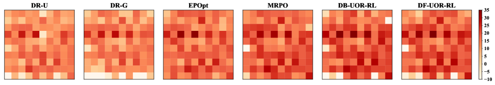
Figure 6: Heat map of $\mathcal{E}_{1}$ in sub-ranges (Reacher). The x-axis and y-axis denote body length and body size, respectively. The ranges of these two parameters are chosen as in Table 1, and are evenly divided into 10 sub-ranges for each one.

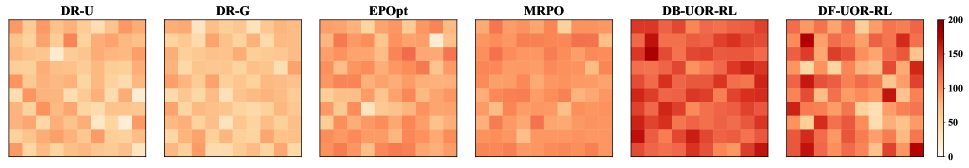
Figure 7: Heat map of $\mathcal{E}_{1}$ in sub-ranges (Humanoid). The x-axis and y-axis denote body length and body size, respectively. The ranges of these two parameters are chosen as in Table 1, and are evenly divided into 10 sub-ranges for each one.

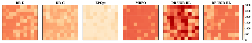
Figure 8: Heat map of $\mathcal{E}_{1}$ in sub-ranges (Walker 2d). The x-axis and y-axis denote body length and body size, respectively. The ranges of these two parameters are chosen as in Table 1, and are evenly divided into 10 sub-ranges for each one.

Due to space limitations, we only show the heat maps of Half Cheetah and Hopper in the main text. Here, we add the heat maps for the remaining tasks(Ant, Humanoid, Reacher and Walker 2d), as shown in Figures 5 to 8.

C.3 Training Curves

Training curves of the baseline algorithms and UOR-RL are shown in Figure 9-13. In the same task, the model of UOR-RL are trained in three different robustness degree $k$, while the baseline models are the same but showing the performance under different metrics. In the process of training the model, the abort condition of training is that the model has reached convergence or has been trained for 1000 iterations.

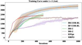
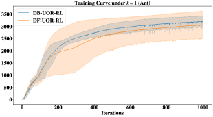
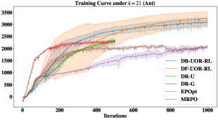
Figure 9: Training Curves (Ant). In the three graphs from left to right, the UOR-RL algorithms are trained under $k=0,1$ and 21, and the y-axis represent the average return of all trajectories, $\mathcal{E}_{1}$ and the average return of worst 10% trajectories respectively.

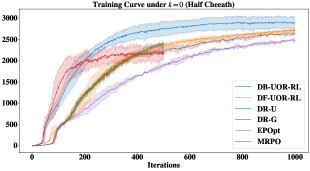
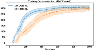
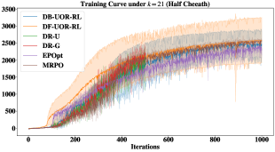
Figure 10: Training Curves (Half Cheetah). In the three graphs from left to right, the UOR-RL algorithms are trained under $k=0,1$ and 21, and the y-axis represent the average return of all trajectories, $\mathcal{E}_{1}$ and the average return of worst 10% trajectories respectively.

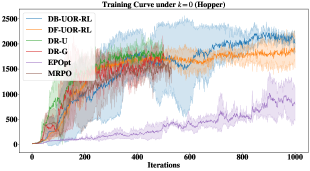
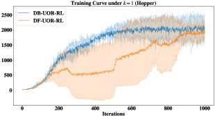
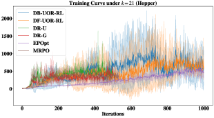
Figure 11: Training Curves (Hopper). In the three graphs from left to right, the UOR-RL algorithms are trained under $k=0,1$ and 21, and the y-axis represent the average return of all trajectories, $\mathcal{E}_{1}$ and the average return of worst 10% trajectories respectively.

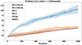
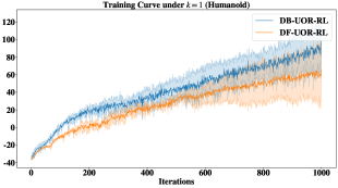
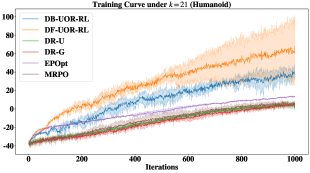
Figure 12: Training Curves (Humanoid). In the three graphs from left to right, the UOR-RL algorithms are trained under $k=0,1$ and 21, and the y-axis represent the average return of all trajectories, $\mathcal{E}_{1}$ and the average return of worst 10% trajectories respectively.

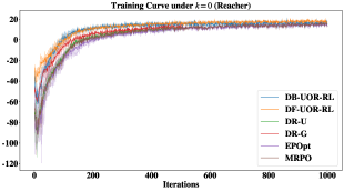
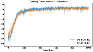
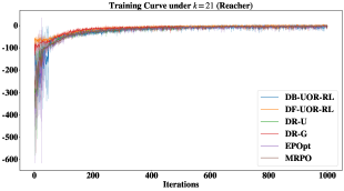
Figure 13: Training Curves (Reacher). In the three graphs from left to right, the UOR-RL algorithms are trained under $k=0,1$ and 21, and the y-axis represent the average return of all trajectories, $\mathcal{E}_{1}$ and the average return of worst 10% trajectories respectively.

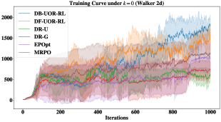
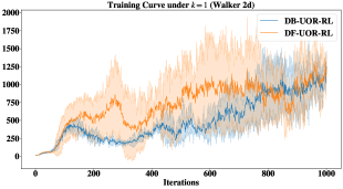
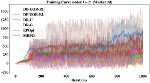
Figure 14: Training Curves (Walker 2d). In the three graphs from left to right, the UOR-RL algorithms are trained under $k=0,1$ and 21, and the y-axis represent the average return of all trajectories, $\mathcal{E}_{1}$ and the average return of worst 10% trajectories respectively.

References

• [1] Volodymyr Mnih, Koray Kavukcuoglu, David Silver, Alex Graves, Ioannis Antonoglou, Daan Wierstra and Martin Riedmiller โ€œPlaying atari with deep reinforcement learningโ€ In arXiv preprint arXiv:1312.5602, 2013
• [2] B Ravi Kiran, Ibrahim Sobh, Victor Talpaert, Patrick Mannion, Ahmad A. Al Sallab, Senthil Yogamani and Patrick Pรฉrez โ€œDeep Reinforcement Learning for Autonomous Driving: A Surveyโ€ In IEEE Transactions on Intelligent Transportation Systems, 2021
• [3] Jens Kober, J Andrew Bagnell and Jan Peters โ€œReinforcement learning in robotics: A surveyโ€ In The International Journal of Robotics Research 32.11 SAGE Publications Sage UK: London, England, 2013, pp. 1238โ€“1274
• [4] David Silver, Guy Lever, Nicolas Heess, Thomas Degris, Daan Wierstra and Martin Riedmiller โ€œDeterministic policy gradient algorithmsโ€ In International Conference on Machine Learning, 2014, pp. 387โ€“395 PMLR
• [5] John Schulman, Filip Wolski, Prafulla Dhariwal, Alec Radford and Oleg Klimov โ€œProximal policy optimization algorithmsโ€ In arXiv preprint arXiv:1707.06347, 2017
• [6] Wolfram Wiesemann, Daniel Kuhn and Berรง Rustem โ€œRobust Markov decision processesโ€ In Mathematics of Operations Research 38.1 INFORMS, 2013, pp. 153โ€“183
• [7] Aravind Rajeswaran, Sarvjeet Ghotra, Balaraman Ravindran and Sergey Levine โ€œEpopt: Learning robust neural network policies using model ensemblesโ€ In arXiv preprint arXiv:1610.01283, 2016
• [8] Chen Tessler, Yonathan Efroni and Shie Mannor โ€œAction robust reinforcement learning and applications in continuous controlโ€ In International Conference on Machine Learning, 2019, pp. 6215โ€“6224 PMLR
• [9] Sebastian Curi, Ilija Bogunovic and Andreas Krause โ€œCombining Pessimism with Optimism for Robust and Efficient Model-Based Deep Reinforcement Learningโ€ In arXiv preprint arXiv:2103.10369, 2021
• [10] Bruno Da Silva, George Konidaris and Andrew Barto โ€œLearning parameterized skillsโ€ In arXiv preprint arXiv:1206.6398, 2012
• [11] Josh Tobin, Rachel Fong, Alex Ray, Jonas Schneider, Wojciech Zaremba and Pieter Abbeel โ€œDomain randomization for transferring deep neural networks from simulation to the real worldโ€ In International Conference on Intelligent Robots and Systems, 2017, pp. 23โ€“30 IEEE
• [12] Sebastian Curi, Felix Berkenkamp and Andreas Krause โ€œEfficient model-based reinforcement learning through optimistic policy search and planningโ€ In arXiv preprint arXiv:2006.08684, 2020
• [13] Yuankun Jiang, Chenglin Li, Wenrui Dai, Junni Zou and Hongkai Xiong โ€œMonotonic robust policy optimization with model discrepancyโ€ In International Conference on Machine Learning, 2021, pp. 4951โ€“4960 PMLR
• [14] Emanuel Todorov, Tom Erez and Yuval Tassa โ€œMuJoCo: A physics engine for model-based controlโ€ In International Conference on Intelligent Robots and Systems, 2012, pp. 5026โ€“5033 IEEE
• [15] Garud N Iyengar โ€œRobust dynamic programmingโ€ In Mathematics of Operations Research 30.2 INFORMS, 2005, pp. 257โ€“280
• [16] Arnab Nilim and Laurent El Ghaoui โ€œRobust control of Markov decision processes with uncertain transition matricesโ€ In Operations Research 53.5 INFORMS, 2005, pp. 780โ€“798
• [17] Michael L. Littman โ€œMarkov games as a framework for multi-agent reinforcement learningโ€ In Machine Learning Proceedings 1994, 1994, pp. 157โ€“163
• [18] Michael L. Littman and Csaba Szepesvari โ€œA Generalized Reinforcement-Learning Model: Convergence and Applicationsโ€ In International Conference on Machine Learning, 1996, pp. 310โ€“318
• [19] Esther Derman, Matthieu Geist and Shie Mannor โ€œTwice regularized MDPs and the equivalence between robustness and regularizationโ€ In Advances in Neural Information Processing Systems, 2021
• [20] Yue Wang and Shaofeng Zou โ€œOnline Robust Reinforcement Learning with Model Uncertaintyโ€ In Advances in Neural Information Processing Systems, 2021
• [21] Kishan Panaganti Badrinath and Dileep Kalathil โ€œRobust reinforcement learning using least squares policy iteration with provable performance guaranteesโ€ In International Conference on Machine Learning, 2021, pp. 511โ€“520 PMLR
• [22] Xuezhou Zhang, Yiding Chen, Xiaojin Zhu and Wen Sun โ€œRobust policy gradient against strong data corruptionโ€ In arXiv preprint arXiv:2102.05800, 2021
• [23] Julien Grand-Clรฉment and Christian Kroer โ€œFirst-Order Methods for Wasserstein Distributionally Robust MDPโ€ In arXiv preprint arXiv:2009.06790, 2020
• [24] Nathan Kallus and Masatoshi Uehara โ€œDouble reinforcement learning for efficient and robust off-policy evaluationโ€ In International Conference on Machine Learning, 2020, pp. 5078โ€“5088 PMLR
• [25] Saurabh Kumar, Aviral Kumar, Sergey Levine and Chelsea Finn โ€œOne Solution is Not All You Need: Few-Shot Extrapolation via Structured MaxEnt RLโ€ In Advances in Neural Information Processing Systems, 2020, pp. 8198โ€“8210
• [26] Kaiqing Zhang, Bin Hu and Tamer Basar โ€œOn the stability and convergence of robust adversarial reinforcement learning: A case study on linear quadratic systemsโ€ In Advances in Neural Information Processing Systems, 2020
• [27] Huan Zhang, Hongge Chen, Chaowei Xiao, Bo Li, Mingyan Liu, Duane Boning and Cho-Jui Hsieh โ€œRobust deep reinforcement learning against adversarial perturbations on state observationsโ€ In arXiv preprint arXiv:2003.08938, 2020
• [28] Huan Zhang, Hongge Chen, Duane Boning and Cho-Jui Hsieh โ€œRobust reinforcement learning on state observations with learned optimal adversaryโ€ In arXiv preprint arXiv:2101.08452, 2021
• [29] Tuomas Oikarinen, Tsui-Wei Weng and Luca Daniel โ€œRobust deep reinforcement learning through adversarial lossโ€ In arXiv preprint arXiv:2008.01976, 2020
• [30] Parameswaran Kamalaruban, Yu-Ting Huang, Ya-Ping Hsieh, Paul Rolland, Cheng Shi and Volkan Cevher โ€œRobust reinforcement learning via adversarial training with langevin dynamicsโ€ In arXiv preprint arXiv:2002.06063, 2020
• [31] Daniel J Mankowitz, Nir Levine, Rae Jeong, Yuanyuan Shi, Jackie Kay, Abbas Abdolmaleki, Jost Tobias Springenberg, Timothy Mann, Todd Hester and Martin Riedmiller โ€œRobust reinforcement learning for continuous control with model misspecificationโ€ In International Conference on Learning Representations, 2020
• [32] Luca Viano, Yu-Ting Huang, Parameswaran Kamalaruban, Adrian Weller and Volkan Cevher โ€œRobust Inverse Reinforcement Learning under Transition Dynamics Mismatchโ€ In Advances in Neural Information Processing Systems, 2021
• [33] Yifang Chen, Simon S Du and Kevin Jamieson โ€œImproved corruption robust algorithms for episodic reinforcement learningโ€ In International Conference on Machine Learning, 2021 PMLR
• [34] Jingkang Wang, Yang Liu and Bo Li โ€œReinforcement learning with perturbed rewardsโ€ In AAAI Conference on Artificial Intelligence, 2020, pp. 6202โ€“6209
• [35] Maximilian Igl, Kamil Ciosek, Yingzhen Li, Sebastian Tschiatschek, Cheng Zhang, Sam Devlin and Katja Hofmann โ€œGeneralization in reinforcement learning with selective noise injection and information bottleneckโ€ In arXiv preprint arXiv:1910.12911, 2019
• [36] Karl Cobbe, Oleg Klimov, Chris Hesse, Taehoon Kim and John Schulman โ€œQuantifying generalization in reinforcement learningโ€ In International Conference on Machine Learning, 2019, pp. 1282โ€“1289 PMLR
• [37] Yinlam Chow, Aviv Tamar, Shie Mannor and Marco Pavone โ€œRisk-sensitive and robust decision-making: a cvar optimization approachโ€ In Advances in neural information processing systems 28, 2015
• [38] Esther Derman, Daniel J Mankowitz, Timothy A Mann and Shie Mannor โ€œSoft-robust actor-critic policy-gradientโ€ In arXiv preprint arXiv:1803.04848, 2018
• [39] Huan Xu and Shie Mannor โ€œDistributionally Robust Markov Decision Processesโ€ In NIPS, 2010, pp. 2505โ€“2513
• [40] Pengqian Yu and Huan Xu โ€œDistributionally robust counterpart in Markov decision processesโ€ In IEEE Transactions on Automatic Control 61.9 IEEE, 2015, pp. 2538โ€“2543