Assessing the Influence of Input Magnetic Maps on Global Modeling of the Solar Wind and CME-driven Shock in the 2013 April 11 Event
Abstract
In the past decade, significant efforts have been made in developing physics-based solar wind and coronal mass ejection (CME) models, which have been or are being transferred to national centers (e.g., SWPC, CCMC) to enable space weather predictive capability. However, the input data coverage for space weather forecasting is extremely limited. One major limitation is the solar magnetic field measurements, which are used to specify the inner boundary conditions of the global magnetohydrodynamic (MHD) models. In this study, using the Alfvén wave solar model (AWSoM), we quantitatively assess the influence of the magnetic field map input (synoptic/diachronic vs. synchronic magnetic maps) on the global modeling of the solar wind and the CME-driven shock in the 2013 April 11 solar energetic particle (SEP) event. Our study shows that due to the inhomogeneous background solar wind and dynamical evolution of the CME, the CME-driven shock parameters change significantly both spatially and temporally as the CME propagates through the heliosphere. The input magnetic map has a great impact on the shock connectivity and shock properties in the global MHD simulation. Therefore this study illustrates the importance of taking into account the model uncertainty due to the imperfect magnetic field measurements when using the model to provide space weather predictions.
Space Weather
Lockheed Martin Solar and Astrophysics Lab (LMSAL), Palo Alto, CA 94304, USA SETI Institute, Mountain View, CA 94043, USA California Institute of Technology, Pasadena, CA 91125, USA
Meng Jinjinmeng@lmsal.com
Due to the inhomogeneous background solar wind and dynamical evolution of the CME, the CME-driven shock parameters change significantly both spatially and temporally when the CME propagates in the heliosphere.
The input magnetic map has great impact on the shock connectivity and shock properties in the global MHD simulation, which is demonstrated in the 2013 April 11 event study.
This study illustrates the model uncertainty due to the imperfect magnetic field observations, which should be considered when the model is used for research or space weather forecasting purposes.
Plain Language Summary
As the origin of space weather, solar wind and coronal mass ejections (CMEs) play an important part in the space weather prediction. Similar as the terrestrial weather forecast, advanced models are developed driven by the available observations. However, the input data coverage for space weather forecasting is extremely limited. One major input data used to drive the solar wind and CME models is the solar surface magnetic field, for which the current telescopes can only observe less than half of the surface therefore assumptions are needed for the rest that leads to different types of magnetic maps. In this study, we quantitatively assess the influence of the two widely used magnetic maps on the global modeling of the solar wind the CME-driven shock in the 2013 April 11 event. Our result suggests that the input magnetic map has a great impact on the simulated background solar wind, CME-driven shock properties, as well as the spacecraft connectivity. Our study illustrates the importance of considering the model uncertainty due to the limited magnetic field coverage when using the model for research or space weather forecasting purposes.
1 Introduction
The broad topic of space weather represents the constantly changing physical conditions in the near-Earth environment, which are significantly influenced by the solar wind and coronal mass ejections (CMEs). Fast CMEs drive shocks in the corona and heliosphere [<]e.g.,¿[]sime87, vour03 that are believed to be responsible for gradual solar energetic particle (SEP) events [<]see reviews by¿[]reames99, desai16 primarily through the diffusive shock acceleration (DSA) mechanism [<]e.g.,¿[]lee83, zank00. Large SEP events can pose major hazards to technology and life in space. If the interplanetary CME is directed at Earth, its embedded magnetic field, especially in the presence of a strong southward-directed component , can interact with Earth’s magnetosphere and trigger non-recurrent geomagnetic storms [Gosling (\APACyear1993)]. Due to their critical importance to space weather prediction, significant efforts have been made in developing physics-based solar wind and CME models [<]see reviews by e.g.,¿[]cranmer17, macneice18, gombosi18. By specifying the radial component of the magnetic field at the inner (photospheric) boundary from observational magnetograms, these models can achieve a steady state solar wind and reproduce with some success the large-scale wind streams at 1 AU. Several simplified analytical flux rope models have also been developed to address the erupting magnetic structure of CMEs [<]e.g.,¿[]titov99, gibson98, titov14, titov18. For example, by initiating a Titov-Démoulin (TD) flux rope, \citeAchip08 simulated the 2003 Halloween CME event and made a quantitative comparison between the synthetic coronagraph images and LASCO observations, in which the strong CME-driven shock was reproduced. \citeAjin17a simulated the 2011 March 7 CME event using the Gibson-Low (GL) flux rope with the Alfvén wave solar model [<]AWSoM;¿[]bart14 from the Sun to 1 AU and performed detailed comparisons with remote-sensing and in-situ observations. The results show that the simulation can reproduce many of the observed features near the Sun and in the heliosphere. A recent study by \citeAtorok18 simulated the famous 2000 July 14 “Bastille Day” eruption using a modified TD (TDm) flux rope [Titov \BOthers. (\APACyear2014)] with the Magnetohydrodynamic Algorithm outside a Sphere model [<]MAS;¿[]lionello13. Starting from a stable magnetic flux rope and initiating the eruption by boundary flows, the simulation is able to reproduce the morphologies of the observed flare arcade, halo CME, and associated EUV wave and coronal dimmings. Although several differences are found between the simulated and observed flux rope at 1 AU, their model successfully captured core structure of the flux rope and the negative Bz component, which led to a very strong geomagnetic storm. Note that there are other approaches for modeling the CME flux rope including the Non-linear Force Free Field extrapolation [<]e.g.,¿[]wiegelmann04, wheatland06, malanushenko14 and magnetofrictional models [<]e.g.,¿[]ballegooijen00, yeates08, cheung12, jiang16.
With increasing sophistication of data-driven models, we are taking steps toward achieving physics-based space weather forecast capability. However, the available input observations for solar wind and CME modeling are severely limited, thereby requiring (often significant) assumptions both for the “missing data” and the physical conditions of the corona. The current data-driven Magnetohydrodynamics (MHD) solar wind models use the photospheric magnetic field observations as inputs. However, all the magnetic field observations (except those started only recently by Solar Orbiter) are from the Sun-Earth line. From this perspective, we can adequately observe only less than one half of the solar surface, and need to make assumptions for the remaining areas, including the far-side and polar regions. There are two major types of magnetic maps that are widely used to drive the solar wind models. One is the synoptic or diachronic magnetic maps that assembles 27-days of magnetic field observations into a single map. One issue with this approach is that the magnetic fields on the same diachronic magnetic map are observed at different times and thus the map contains data which are up to 27-days old. The other type is synchronic magnetic maps that are based on surface flux transport models which simulate the evolution of the surface magnetic elements while assimilating new observations [<]e.g.,¿[]schrijver03. Additionally, a synchronic map may incorporate the newly emerged flux on the far-side of the Sun as inferred from helioseismology [Lindsey \BBA Braun (\APACyear1997), Braun \BBA Lindsey (\APACyear2001), González Hernández \BOthers. (\APACyear2007)]. A preliminary study shows that by including the far-side flux in the Air Force Data Assimilative Photospheric Flux Transport (ADAPT) - Wang-Sheeley-Arge (WSA) model, the observed solar wind conditions could be better reproduced [Arge \BOthers. (\APACyear2013)]. However, doing so is not straightforward given the number of assumptions needed for the total fluxes and tilt angles of such emerging flux elements. Since most of the current solar wind models rely on either of these two types of magnetic maps, it is important to quantitatively evaluate the differences in ambient solar wind solutions as obtained using the diachronic orsynchronic magnetic map inputs. We note that some studies have examined the uncertainties of the solar wind solutions due to magnetic data from different observatories [Gressl \BOthers. (\APACyear2014), Riley \BOthers. (\APACyear2014), Jian \BOthers. (\APACyear2015), Hayashi \BOthers. (\APACyear2016)]. There are also recent studies that compare the solar wind solutions from the diachronic and synchronic magnetic inputs based on either PFSS model [<]e.g.,¿[]wallace19, caplan21 or MHD models [<]e.g.,¿[]linker17, lfw21.
However, most of the previous studies have focused on comparing the ambient solar corona and wind solutions, and not transient structures, driven by the different magnetic inputs. It is widely known that the ambient solar wind can have significant influence on the evolution of the CME and the properties of the CME-driven shock wave, as has been studied both in simulations [<]e.g.,¿[]riley99, riley03, ods04, jacobs05, hosteaux19 and in observations [<]e.g.,¿[]gopalswamy00, temmer11. Here, we propose to investigate the influence of different background solar wind solutions, due to the different magnetic inputs (i.e., diachronic vs. synchronic), on the CME properties in 3D. In particular, the parameters of the CME-driven shock (e.g., compression ratio, Mach number, shock speed, and shock angle ) are critical for understanding the particle acceleration in gradual SEP events. However, these shock parameters are difficult to determine directly from remote sensing observations [<]e.g.,¿[]rouillard16, lario17, kwon18. Furthermore, the field line connectivity plays an important role in understanding the in-situ SEP observations [<]e.g.,¿[]lario17, although it is also difficult to determine from current measurements. Therefore, to infer the link between the observer and the shock, most of the current SEP modeling efforts use Parker-spiral magnetic connectivity outside the source surface, which is often set at the heliocentric distance of 2.5 R⊙. Due to the simplicity of this technique, such models do not always explain the observed characteristics of some SEP events [<]e.g.,¿[]cairns20. With the dynamic magnetic connectivity and shock parameters available from an MHD model, additional information relevant to the shock acceleration can be obtained through a physics-based approach.
In this study, we quantitatively assess the influence of the magnetic input, by modeling the CME on 2013 April 11 and its shock, which was associated with an SEP event [<]e.g.,¿[]cohen14, lario14. This article is organized as follows. In Section 2, we describe the models and methods used in this study, followed by results in Section 3 and discussion and conclusions in Section 4.
2 Methodology
2.1 Data Description
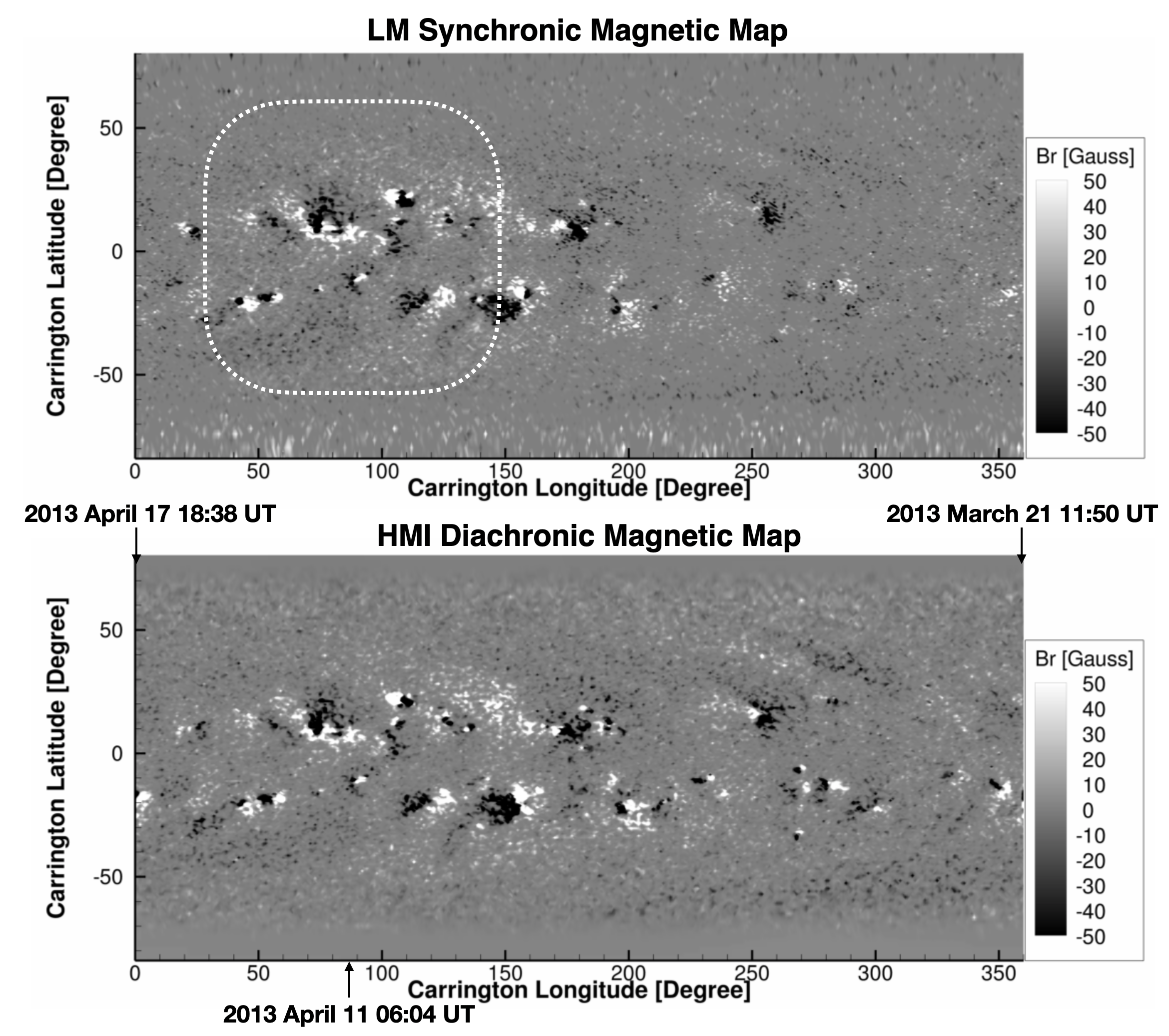
The CME was clearly associated with an M6.5 class flare starting at 06:55 UT in AR 11719 (N07E13, Carrington longitude 73∘). At the time, the Carrington longitude for Earth, STEREO A (STA), and STEREO B (STB) were 86∘, 219∘, and 304∘, respectively. We use both diachronic and synchronic magnetic maps based on SDO/HMI observations [Schou \BOthers. (\APACyear2012)] to specify the model’s inner boundary condition of magnetic field. The synchronic magnetic map in use is maintained at the Lockheed Martin Solar and Astrophysics Laboratory and based on a flux transport model [Schrijver \BBA DeRosa (\APACyear2003)], which assimilates new observations within 60∘ from disk center. These magnetic maps are updated every six hours and can be downloaded directly from the PFSS package in SSWIDL. The latest documentation of the LM flux transport model can be found online (https://www.lmsal.com/forecast/surfflux-model-v2/). The diachronic magnetic map is obtained from the Stanford HMI Carrington Rotation Synoptic Charts. At each Carrington longitude in the magnetic map, the data are averaged from 20 contributing magnetograms made within 2 hours of central meridian passage (i.e., 1.2∘ of the central meridian) with the outliers (values which depart from the median by 3) removed. See \citeAliu17 for more details. We choose the HMI diachronic magnetic map with polar field correction [Sun (\APACyear2018)] accessible at JSOC (http://jsoc.stanford.edu/) under dataseries hmi.synoptic_mr_polfil_720s (36001440 resolution).
2.2 Solar Wind and CME Models
The MHD solar wind model used in this study is the Alfvén Wave Solar Model [<]AWSoM;¿[]bart14, which is a data-driven model with a domain starting from the upper chromosphere and extending to the corona and heliosphere. The AWSoM model has been implemented at NASA’s Community Coordinated Modeling Center (CCMC). The inner boundary condition of the magnetic field can be specified by different magnetic maps as mentioned in §1. The inner boundary conditions for electron and proton temperatures and and number density are set to be 50,000 K and 21017 m-3. The fixed density and temperature at the inner boundary do not otherwise have an evident influence on the global solar corona and wind solution [Lionello \BOthers. (\APACyear2009)]. The detailed model validation on coronal density has been conducted by comparing numerical results with spectral line (e.g., EIS and SUMMER) observations [Oran \BOthers. (\APACyear2013)], EUV line intensities [Jin \BOthers. (\APACyear2017)], and more recently through the density derived from the Differential Emission Measure Tomography [Sachdeva \BOthers. (\APACyear2019)]. The Parker solution [Parker (\APACyear1958)] is used to specify the initial conditions for the solar wind plasma, while the initial magnetic field is based on the Potential Field Source Surface (PFSS) model with the Finite Difference Iterative Potential Solver [<]FDIPS;¿[]toth11. In this study, the source surface is set at 2.5 R⊙. The global solar wind solution is obtained by coupling the solar corona (SC; from 1 to 24 R⊙) and inner heliosphere (IH; from 18 to 250 R⊙) components within the Space Weather Modeling Framework [<]SWMF;¿[]toth12.
Alfvén waves are prescribed as outgoing Alfvén wave energy density that scales with the surface magnetic field. The solar wind is heated by a phenomenological description of Alfvén wave dissipation and accelerated by thermal and Alfvén wave pressure. Electron heat conduction (both collisional and collisionless) and radiative cooling are also included in the model, which are important for creating the solar transition region self-consistently. In addition, the model electron and proton temperatures are treated separately for producing physically correct solar wind and CME structures (e.g., CME-driven shocks), in which the electrons and protons are assumed to have the same bulk velocity but heat conduction is applied only to electrons due to their much higher thermal velocity [Manchester \BOthers. (\APACyear2012), Jin \BOthers. (\APACyear2013)]. By introducing the phenomenological description of Alfvén wave dissipation as well as the wave reflection and heat partitioning between the electrons and protons based on the results of linear wave theory and stochastic heating [Chandran \BOthers. (\APACyear2011)], the AWSoM model has demonstrated the capability to reproduce the solar corona environment with three free parameters that determine the Poynting flux (), the wave dissipation length (), and the stochastic heating parameter () [van der Holst \BOthers. (\APACyear2014)].
To initiate a CME eruption, we use the Gibson-Low (GL) flux rope model [Gibson \BBA Low (\APACyear1998)] which has been successfully used in numerous modeling studies of CMEs [<]e.g.,¿[]chip04a, chip04b, lugaz05a, lugaz05b, schmidt10, chip14. Analytical profiles of the GL flux rope are obtained by finding a solution to the magnetohydrostatic equation with the solenoidal condition . To get the solution, a mathematical stretching transformation is applied to an axisymmetric, spherical ball of twisted flux with diameter centered at relative to the heliospheric coordinate system. The field of can be expressed by a scalar function and a free parameter that determines the magnetic field strength [Lites \BOthers. (\APACyear1995)]. The flux rope acquires a tear-drop shape of twisted magnetic flux after the transformation. Also, Lorentz forces are introduced that lead to a density-depleted cavity in the upper portion and a dense core at the lower portion of the flux rope. This flux rope structure mimics the 3-part density structure of the CME seen in observations [Illing \BBA Hundhausen (\APACyear1985)]. The GL flux rope profiles are then superposed onto the steady-state solar wind solution: i.e. , , . The combined background-flux rope system is in a state of force imbalance, and thus erupts immediately when the simulation is advanced forward in time. The GL flux rope is mainly controlled by five parameters: the stretching parameter, , determines the flux rope shape; the distance of torus center from the center of the Sun, , determines the initial position of the axisymmetric flux rope before it is stretched; the radius of the flux rope torus, , determines the flux rope size; the flux rope field strength parameter, , determines the magnetic field strength of the flux rope; and a helicity parameter to determine the positive (dextral) /negative (sinistral) helicity of the flux rope [Jin \BOthers. (\APACyear2017), Borovikov \BOthers. (\APACyear2017)]. \citeAjin17b developed a new method, Eruptive Event Generator Gibson-Low (EEGGL), to calculate GL flux rope parameters through a handful of observational quantities (i.e., magnetic field of the CME source region and observed CME speeds from white-light coronagraphs) so that the modeled CMEs can propagate with the desired CME speeds near the Sun.
2.3 Summary of Approach
To quantitatively assess the influence of magnetic input on the global modeling, we choose two different magnetic maps: the Lockheed Martin (LM) synchronic magnetic map for 2013 April 11 06:04:00 UT (referred to as input to Case I) and the diachronic Carrington magnetic map of CR2135 (referred to as input to Case II). Both types of magnetic maps have been widely used in the solar and heliospheric physics community for space weather nowcast/forecast purposes. The original magnetic maps are first resized to 360180 resolution that matches simulation grid while preserving the flux. For the LM synchronic map, this is done directly through the PFSS package in SSWIDL. For the HMI diachronic map, we resize the data from the original map in 36001440 resolution. In addition, both magnetic maps have flux imbalance (i.e., zero-point error), which is calculated to be -6.91021 Mx (-2% of the total unsigned flux) and 5.41021 Mx (1.3% of the total unsigned flux) for the LM synchronic map and HMI diachronic map respectively. This zero-point error is corrected by removing the average field (i.e. monopole) from the original magnetic maps [Tóth \BOthers. (\APACyear2011)]. Other than this correction, we do not apply any scaling factor to the input magnetic maps in this study.
Figure 1 shows the two magnetic maps used in this study. The LM synchronic magnetic map contains magnetic field observations only 60∘ from the disk center on 2013 April 11 06:04:00 UT (marked with white dotted box in Figure 1) while the rest of the magnetic map is based on the flux transport model. Due to the different methods used to produce these magnetic maps mentioned in §2.1, one can see evident differences between the two magnetic maps for areas with longitude 200∘. However, the magnetic fields around the source region (73∘) are similar between the two maps. To quantitatively compare the two magnetic maps, we further calculate the unsigned flux for both the whole map and the assimilating window, and the mean polar field strength. The results are summarized in Table 1. First, we need to note that for newly assimilated observation (marked as white dashed window in Figure 1) in the LM synchronic map, the HMI flux is multiplied by a factor of 1.4 in order to match the previous MDI observations [Liu \BOthers. (\APACyear2012)]. Even with that enhanced magnetic flux, the total unsigned flux in the synchronic map (3.51023 Mx) is still 17% less than that in the diachronic map (4.11023 Mx), which is mainly due to more and stronger magnetic structures involved in the diachronic map outside the assimilating area of the synchronic map where the flux diffuses in the flux transport model. However, we find that the total unsigned flux within the assimilating window is similar between the two maps (1.31023 Mx for synchronic map vs. 1.21023 Mx for diachronic map). Considering the factor of 1.4 applied to the field in the assimilating window of synchronic map, this also means there must be considerable field evolution around 2013 April 11 (e.g., newly emerged fluxes after 2013 April 11). Note that based on the start/end times of Carrington Rotation 2135, the assimilating window area in the synchronic map corresponds to 9 days of observation (2013 April 6 to 2013 April 15) in the diachronic map. On the other hand, similar unsigned flux also means that about the same amount of Poynting flux is initiated in the AWSoM model for heating the corona. Another noticeable difference between the two maps is the polar field (Carrington latitude 60∘). For LM synchronic map, the polar field is simulated from the flux transport model over many solar rotations. For the HMI diachronic map used here, the polar field is extrapolated from previous observations when part of the polar region could be seen due to the Sun’s tilt angle. Therefore, we can see many small-scale structures in the polar region of the synchronic map while the polar field in the diachronic map is smoothed due to the extrapolation. Nevertheless, we found that the mean magnetic fields in the south polar region are very similar (2.7 Gauss for synchronic map vs. 2.6 Gauss for diachronic map). For the north polar region, the synchronic map has a lower mean field of -1.5 Gauss comparing with the -2.2 Gauss field in the diachronic map.
We run two steady-state simulations with the inner boundary condition of the magnetic field specified by the two different magnetic maps. After reaching the steady-state, we initiate a CME eruption by inserting a Gibson-Low flux rope into both steady-state solutions and integrate the model equations forward in time. The GL flux rope parameters are identical in the two simulation cases. We run the two cases for a duration of one hour in total simulated time, trace the shock location in 3D and calculate the shock parameters in order to compare the two simulations.
The 3D shock front is determined by computing the derivative of entropy along the radial rays originating from the center of the Sun. The entropy is evaluated as where is the proton temperature, is the plasma density, and is the polytropic index (=5/3). Once the shock front is determined, the shock normal is calculated by using the magnetic coplanarity condition [Lepping \BBA Argentiero (\APACyear1971), Abraham-Shrauner (\APACyear1972)]:
| (1) |
where 1 and 2 represent the shock downstream and upstream conditions, respectively. The shock speed is determined by the conservation of mass across the shock: . The shock Alfvén Mach number is defined as , where is the local Alfvén speed. The shock angle is obtained by measuring the angle between the upstream magnetic field and the shock normal. To get the shock connectivity to different spacecraft locations, we extract field lines from the outer boundary of SC at 24 R⊙ to the surface of the Sun. Since in this study, we did not extend the domain to include the IH component for the CME simulation, the connectivity from the spacecraft locations to the outer boundary of SC is determined by the steady-state solution that did include the heliospheric domain. Considering the relative short simulation time, this simplification has minimal influence on our results. To get the shock evolution profiles, for each time step (in 1 minute temporal resolution), we extract the shock parameters on the shock surface closest to the spacecraft-connecting field lines.
3 Results
3.1 Comparison of Steady-state Solutions
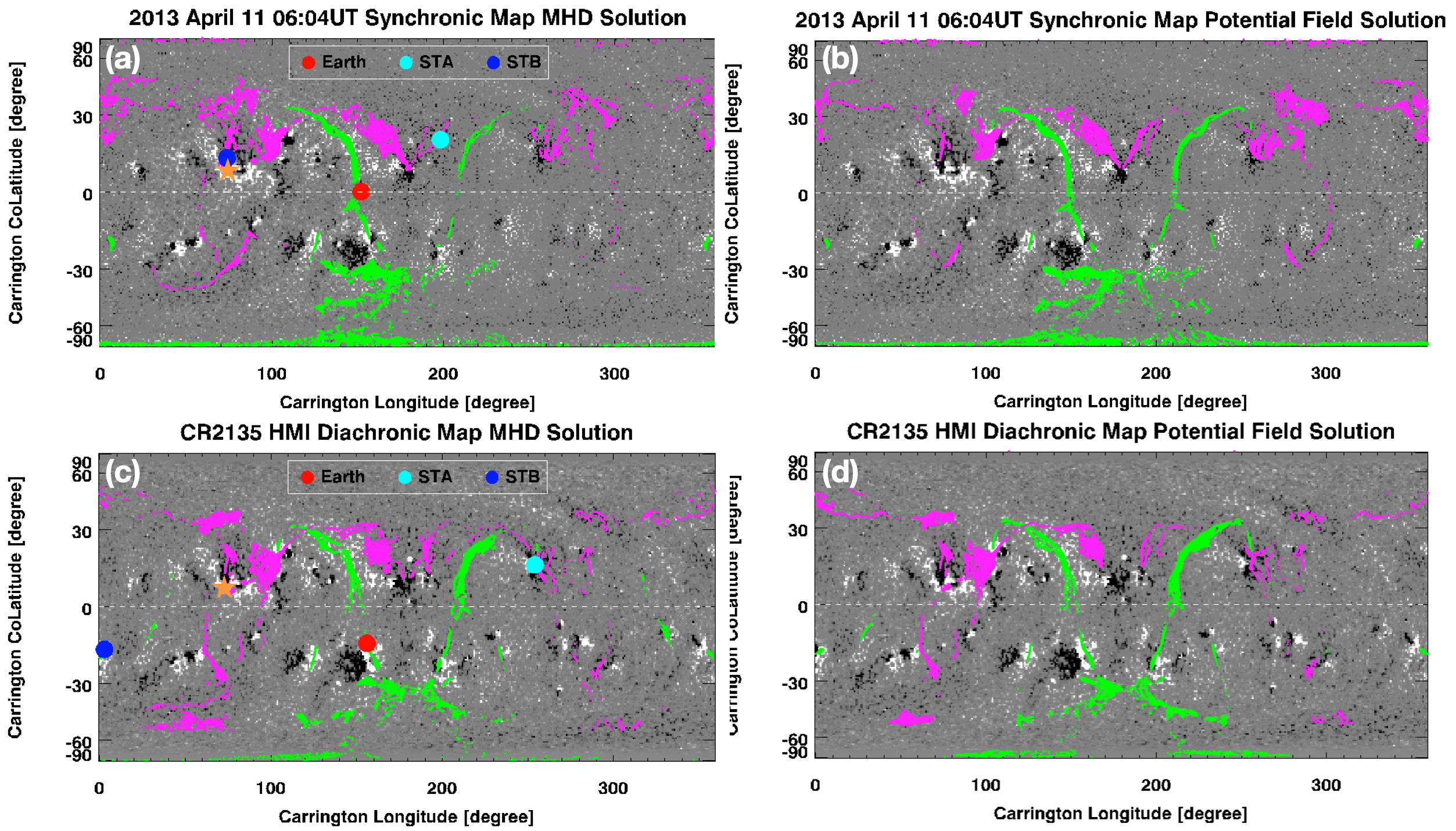
In order to compare the two steady-state solar wind solutions constructed using the two magnetic maps, we calculate the locations of the positive (marked in green) and negative (marked in purple) open flux from both MHD and PFSS solutions as shown in Figure 2. The open flux is identified by tracing the field lines from the outer boundary at 24 R⊙ in the simulations in a uniform latitude/longitude grid with one degree resolution back to the surface of the Sun. To quantitatively compare the results, we also calculate the open field area for both the positive and negative polarities and the results are summarized in Table 1. For both of the magnetic maps, the MHD and PFSS solutions are quite similar with the total open area slightly higher in the PFSS solution. The similarity between the MHD and PFSS solutions also suggests that the inherent properties of the different magnetic maps play a major factor in generating the different topological features instead of other model-related parameters. However, we need to note that the statistics in this particular case may not be generalized for all the MHD/PFSS models. Other adjustable parameters of both MHD and PFSS models could influence the open field area. For example, a lower source surface radius in the PFSS model could lead to larger open field area [Caplan \BOthers. (\APACyear2021)], while the coronal heating (i.e., Alfvén wave heating) related parameters in the MHD model could also influence the field opening [Linker \BOthers. (\APACyear2017)]. Comparing between the synchronic and diachronic map, both MHD and PFSS solutions show similar total open field area. However, there are also noticeable differences: For example, the positive flux area is larger in Case II than in Case I, while the negative flux area is larger in Case I.
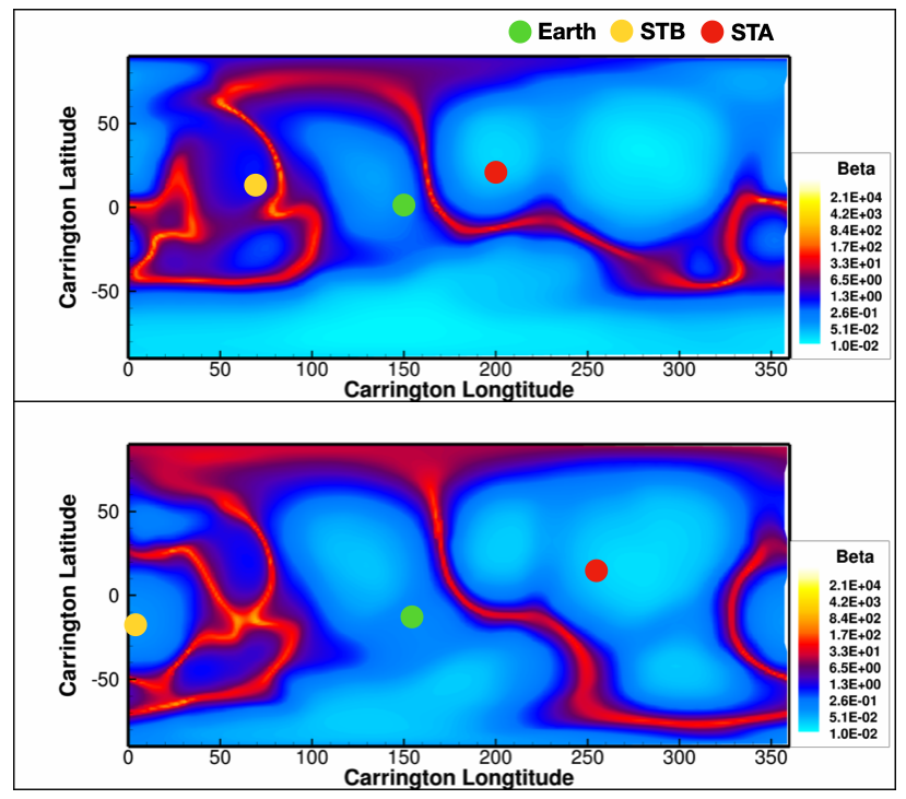
We extract the field lines connecting to Earth, STEREO A (STA), and STEREO B (STB) and mark the footpoints on the magnetic maps (indicated with colored circles). It is also apparent in Figure 2 that the connectivity to the three 1 AU locations are quite different between the two solutions. For Earth, although both calculated footpoints are around the same longitude, they are 20∘ different in latitude. For STA, the footpoints are at approximately the same latitude in northern hemisphere, but they differ by 50∘ in longitude. The largest difference is found in the STB footpoints, which vary by 70∘ in longitude and 40∘ in latitude. Moreover, the polarities are different for the two STB footpoints. In Figure 3, the plasma- at 2.5 R⊙ from the MHD solutions are shown for the two cases; the location of the heliospheric current sheet (HCS) is indicated by the high plasma- values. Although there are a number of differences between the two cases, of note is that STB’s footpoint shifts from one side of the HCS to the other (this is not the case for STA or Earth). This connectivity difference significantly influences the shock profile evolution after the CME eruption observed at each location, as is discussed in the next section.
3.2 Comparison of CME-driven Shocks
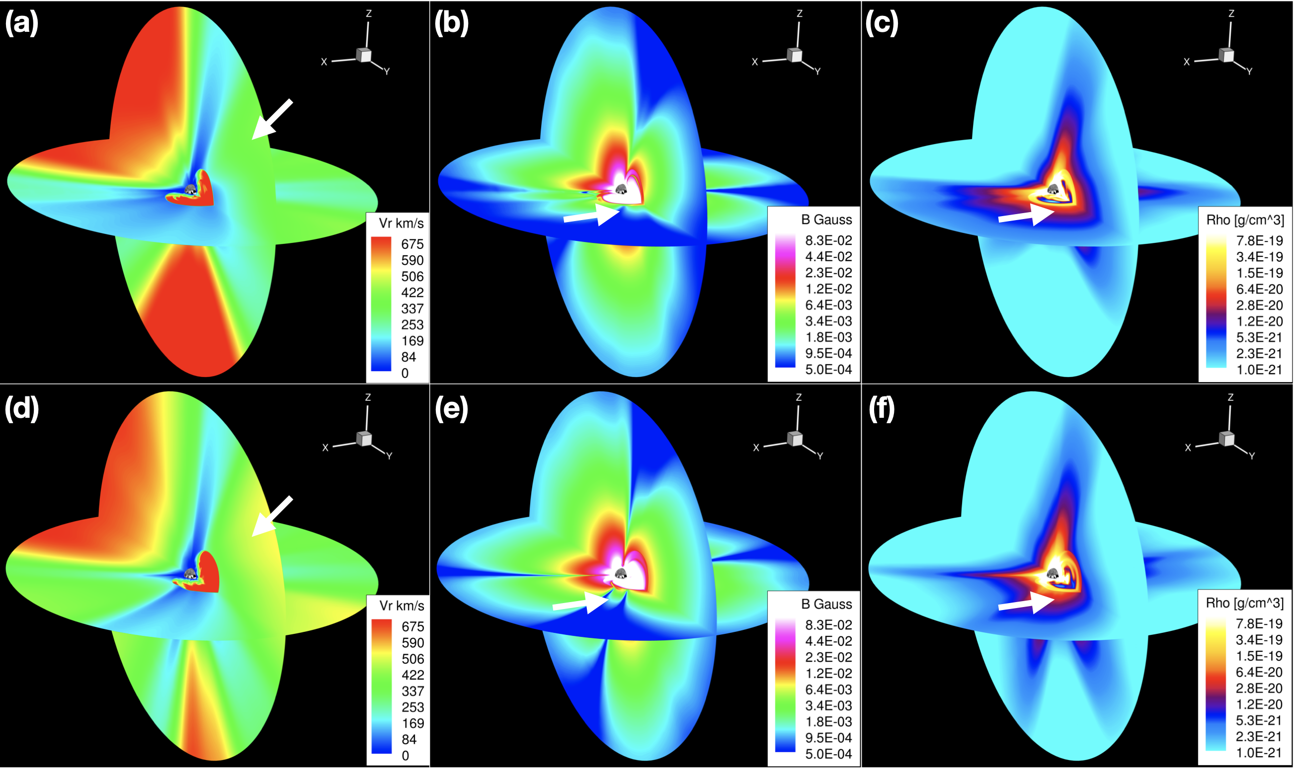
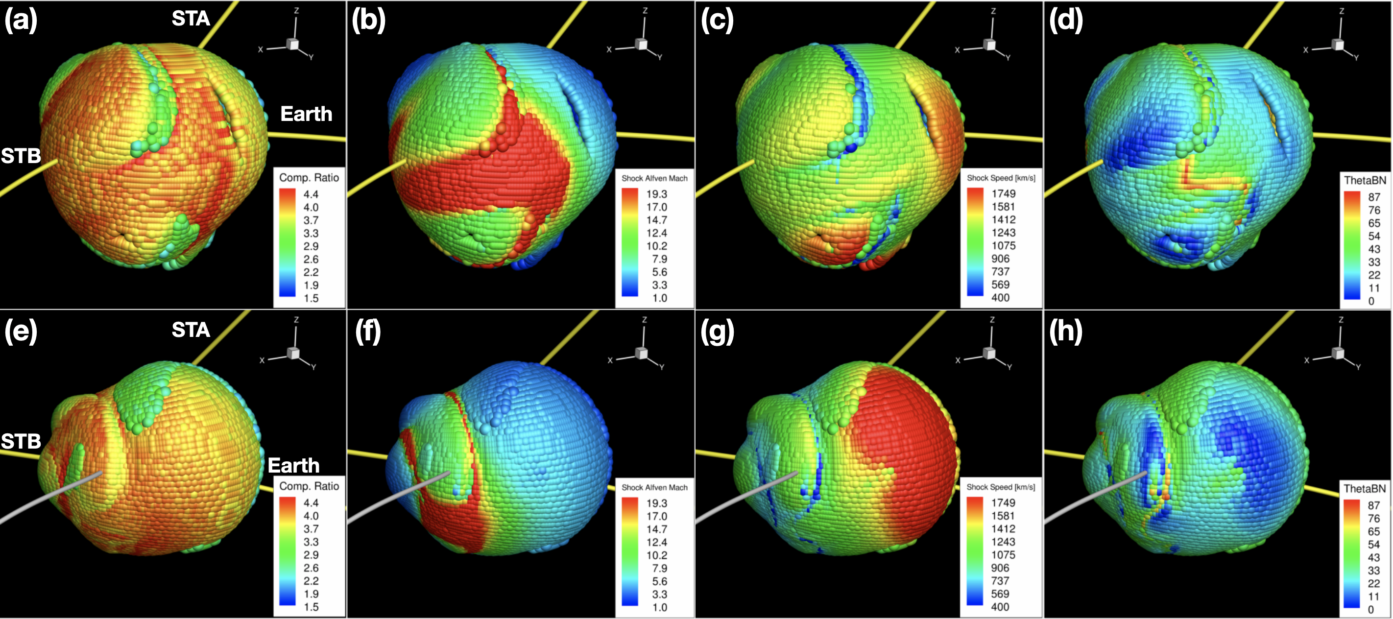
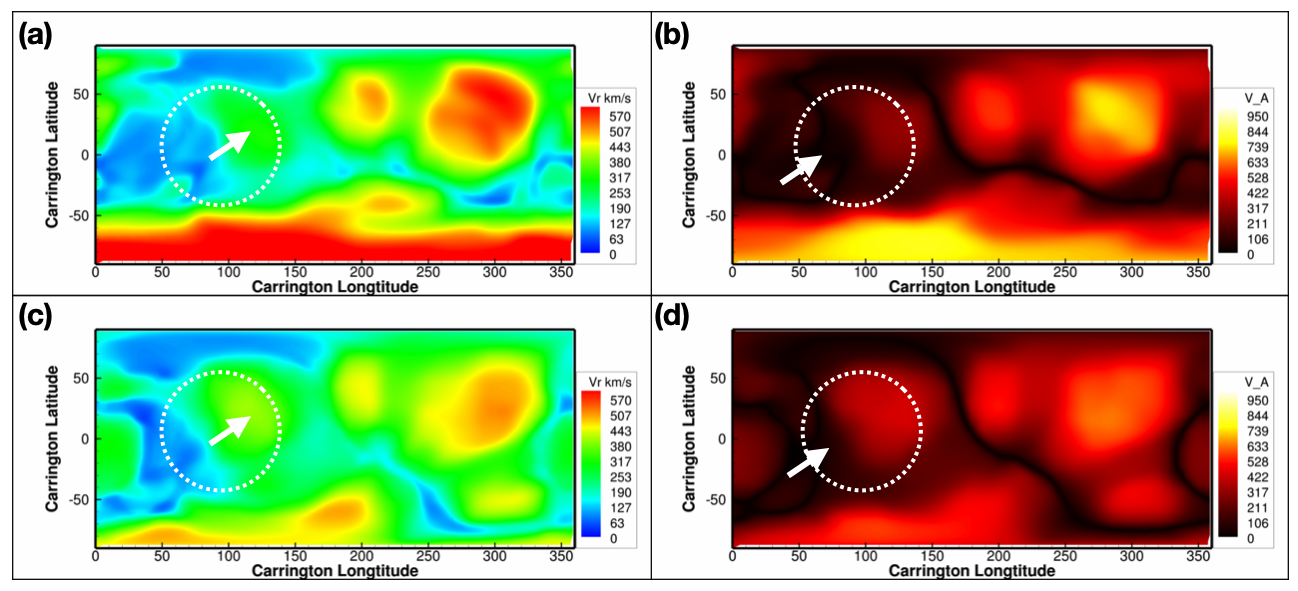
With the same CME flux rope running through the two different ambient coronal and solar wind solutions, we obtain two CME simulation cases. The Cartesian coordinate system used in the simulation is the heliographic rotating coordinates (i.e., Carrington coordinates) with the X-axis pointing to the Carrington longitude 0∘ and Y-axis pointing to the Carrington longitude 90∘. In Figure 4, we show radial velocity field, total magnetic field strength, and plasma density on the = 0 and = 0 planes at = 30 minutes for the two CME simulation cases, from which we can also see the background solar wind conditions based on the two magnetic maps. In general, there are similar patterns we can identify between the two cases. However, there are also evident differences in the two solar wind conditions that lead to different shock parameters as discussed below. In Figure 5, we show the 3D shock parameters (compression ratio, shock Alfvén Mach number, shock speed, and shock angle ) extracted from the two cases at 30 minutes. The yellow field lines represent the connectivity to Earth, STA, and STB. Due to the inhomogeneous background solar wind, the CME-driven shocks in both cases are highly structured in shape and all the shock parameters vary significantly across the shock surface. By comparing the two cases with different magnetic field inputs, we can see several major differences: 1) The morphology of the shock surface, in that the latitudinal expansion is larger in Case I than in Case II; 2) The spatial distribution of Mach number along the shock surface is evidently different between the two cases. We find that the high Mach numbers in both cases are due to the smaller local Alfvén speeds in the shock upstream as shown in Figure 6b and d (area indicated by white arrows). These smaller Alfvén speeds are related to both low magnetic field strength (Figure 4b and e) and enhanced plasma density (Figure 4c and f); 3) The spatial distribution of shock speed differs. The larger shock speed found at the leading front of the shock surface in Case II is related to the faster background solar wind around that region (marked by white arrows in Figure 4a and d). See also the higher solar wind speed in the upstream of the shock in Case II (Figure 6a and c). Finally, the footpoint differences seen in Figure 2 result in the Earth, STA, and STB being connected to different parts of the shock in the two cases.
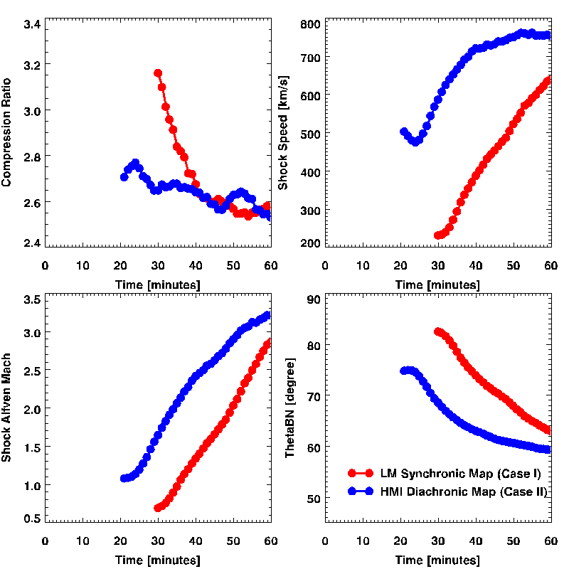
To quantitatively evaluate the differences of the CME-driven shock parameters in the two cases, we derive the evolution of shock parameters connected to the Earth and STB locations in the two cases and show the results in Figure 7 and 8. Note that no shock connection is developed for STA in either cases and therefore, the STA profiles are not shown. The temporal resolution of the shock profiles is 1 minute. We found that the shock compression ratio calculated for STB location in Case I is slightly larger than 4 (strong shock limit), which is due to the nonideal process (e.g., heat conduction) involved in the MHD model. Also, we need to note that due to the unstable flux rope insertion used in this study, the shock parameters derived at the beginning could be unrealistically stronger, especially right in front of the flux rope driver. However, as the flux rope starts interacting with the global corona, the resulting CME tends to acquire a speed that agrees with the observations reasonably well as found in our previous studies [Jin \BOthers. (\APACyear2017), Jin \BOthers. (\APACyear2018)].
As we mentioned before, the footpoints connected to Earth in the two cases are around the same heliospheric longitude; this results in similar trends in the evolution of the shock parameters for the two cases. Also, the shock has a perpendicular nature in both cases throughout the first hour of the simulation. However, comparing the absolute values of the shock parameters, they are quite different between the two cases. In addition, the shock connection time is different in the two cases; in Case I, the connection is developed 10 minutes later than in Case II with the connection to Earth established only 20 minutes after the eruption onset.
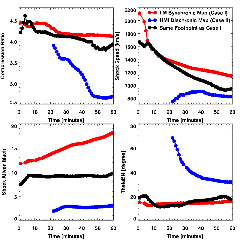
In contrast, due to the large difference in the locations of the STB footpoints, the CME-driven shock properties connecting to STB in the two cases are significantly different as shown in Figure 8. The shock connecting to STB in Case I is a much stronger shock than that in Case II with a much higher compression ratio, shock Alfvén Mach number, and shock speed. Also, the shock in Case I has a parallel nature (i.e., shock angle 20∘) while the shock in Case II is more oblique and has a perpendicular nature in the initial 10 minutes after first contact. Furthermore, the connection in Case I is established 20 minutes earlier than in Case II, which might have an effect on the properties of the resulting SEP event. For example, based on the DSA theory [Drury (\APACyear1983)], the instantaneous particle spectral index depends only on the shock compression ratio and the higher shock compression ratio in Case I will lead to a harder SEP spectra. The higher shock compression ratio and quasi-parallel nature found in the Case I also suggests the shock is a more efficient accelerator than in the Case II [Ding \BOthers. (\APACyear2020)]. However, due to the complex physical processes of the particle acceleration and transport involved, to quantitatively link the shock properties near the Sun to the SEP spectra at 1 AU requires advanced coupling between the MHD model and a particle acceleration/transport model [Young \BOthers. (\APACyear2021), G. Li \BOthers. (\APACyear2021)], which is beyond the scope of this work and will be examined in a future study.
As shown in Figure 5, one major reason for the completely different shock profiles connecting to STB is the field line connectivity in the two cases, which results in STB being connected to different parts of the shock. In Case I, STB connects more closely to the front of the shock, while in Case II the connection is closer to the shock flank. To make a more comprehensive comparison, we also extract the field line with a footpoint rooted in the same region as the field line connecting to STB in Case I (shown as a white field line in Figure 5e-h). The shock evolution profile from this extra field line is overlaid in Figure 8 (marked in black). We can see that when comparing shock profiles around the similar longitude/latitude location in the two cases, the shock parameters and their evolution are more similar mainly due to the same flux rope driver initiated in the two simulations. However, we want to emphasize that this similarity does not otherwise reconcile the issue we raised in this study as the different spacecraft connectivity in the two cases is largely attributable to different input magnetic maps. Furthermore, even at a similar location on the shock surface, certain shock parameters (e.g., Shock Alfvén Mach number) still show clear differences between the two cases, which is caused by the different background solar wind solutions.
4 Discussion & Conclusions
In the previous section, we have shown that the CME-driven shock parameters and connectivity can be significantly different when different types of magnetic maps are used to drive global MHD models. Here, we briefly discuss how these differences could influence our interpretation of observations in the 2013 April 11 SEP event.
As shown in Figure 2, one major difference found in field line connectivity between the two cases is the footpoint connecting to STB. In Case I, we can see that the STB-connecting field line can be traced back to the flare site, while in Case II, the footpoint is far from the flare site. The SEP observations of this event show that the Fe/O ratio is higher at STB than at Earth [Cohen \BOthers. (\APACyear2014)]. Based on Case I, one possible explanation for the high Fe/O ratio could be that there is a direct contribution from the flare-accelerated, Fe-rich material [Cane \BOthers. (\APACyear2003), Cane \BOthers. (\APACyear2006)]. However, Case II does not support this interpretation as the STB and Earth footpoints have about the same longitudinal separation from the source region and therefore presumably more likely to measure similar Fe/O ratios.
Another feature that can be compared with observations is the shock-connection time. We found that in Case I, STB develops connection to the shock 30 minutes earlier than Earth, while in Case II, STB and Earth develop connections to the shock around the same time (20 minutes after the eruption). The shock-connection time can be related to the particle release time calculated from the SEP in-situ observations. For this event in particular, \citeAlario14 found that the estimated proton release time at STB from velocity dispersion analysis is 07:10 UT4 minutes and 07:58 UT9 minutes at Earth, which suggests that STB developed a connection to the shock earlier than the Earth did by 4813 minutes, consistent with the 30 minutes found in Case I.
However, there are also features the two cases agree on. For example, in both cases, the shock connecting to STB is stronger than the shock connecting to Earth. This feature is consistent with the SEP observations that the energy spectra of He, O, and Fe are harder at STB than at Earth [Cohen \BOthers. (\APACyear2014)]. Also, the shock geometry connecting to the Earth location has a quasi-perpendicular nature (i.e., shock angle 45∘) in both cases, although the shock is more oblique in Case I. For the shock connecting to STB, although the shock starts with a quasi-perpendicular nature in Case II, the shock angle quickly decreases with time. After 40 minutes, the shock in both cases has a quasi-parallel nature with Case II more oblique.
We need to note that in this study, we are mainly focused on the influence of input magnetic maps on the MHD model output. But there are other parameters that could influence the modeling result. For example, the coronal heating parameters used in the MHD model (e.g., input wave energy density and length scale of energy dissipation) can have great influence on the final field topology [Linker \BOthers. (\APACyear2017)]. The enhanced coronal heating or shorter dissipation length could lead to more field opening in the MHD simulation. For the PFSS model, when using a lower source surface location, it also leads to more open field in the solution [Caplan \BOthers. (\APACyear2021)]. Moreover, the solar corona is a continuously changing environment, which may not be correctly represented by either PFSS model or a relaxed steady-state MHD solution. In contrast, the global magneto-friction model could provide an approach to account for such time-dependent factors [Yeates \BOthers. (\APACyear2010), Cheung \BBA DeRosa (\APACyear2012), Fisher \BOthers. (\APACyear2015)]. Last but not least, the CME flux rope models used for initiating the eruptions could also play an important role for different CME-driven shock properties. Therefore, more work is needed for a comprehensive assessment on these factors and their relative importance on the model output.
In this study, using the CME on 2013 April 11 associated with a SEP event as an example, we demonstrated how the choice of magnetic inputs can result in significantly different simulated background solar wind and, therefore, the CME-driven shock parameters and spacecraft connectivity in a global MHD model. There are multiple differences in the details of the synchronic and diachronic maps that may contribute to the differences in the results of the two cases: the characteristics of the active regions (especially on the far-side), the strength of the polar field, and the flux imbalance between the polar regions. For the case in this study, we found that the flux imbalance between the two polar regions is much larger for the LM synchronic map (ratio of 1.8) than for the diachronic map (ratio of 1.2). This flux imbalance could influence the global field topology, position of the HCS, and magnetic field connectivity. The different polar fields also have impact on the resulting solar wind speed. As shown in Figure 4 and Figure 6, the region of fast solar wind in the south is much wider and stronger in Case I than in Case II.
Given the many differences between the two cases resulting from the two magnetic map inputs, one could potentially use the multi-wavelength remote-sensing observations and in-situ measurements to help select the more appropriate input magnetic map, for instance, by comparing the on-disk structures shown in the EUV observations (e.g., coronal holes) or the large-scale solar wind structures (e.g., helmet streamers) seen in the white-light observations. In addition, the in-situ measurement of plasma parameters could be used to validate the solar wind solutions. However, we want to emphasize that the purpose of this study is not to distinguish which type of magnetic map is better but rather to illustrate the model uncertainty due to the imperfect magnetic field observations, which has to be taken into account whether the model is utilized for space weather prediction or for scientific research. In the meantime, we suggest that the magnetic input source should be explicitly mentioned in research papers that use global MHD models and the associated model uncertainties be discussed wherever possible. This study also emphasizes the need to have better observational coverage of the solar magnetic field for improving space weather forecasting, and should be a substantial consideration in the development of future missions. All the differences in the evolution of shock parameters could lead to significantly different inferred particle acceleration processes and result in different expected SEP spectra, complicating the interpretation of the SEP observations.
Acknowledgements.
We are very grateful to the referees for invaluable comments that helped improve the paper. We thank Marc DeRosa at LMSAL for the helpful discussion on the LM synchronic magnetic maps. MJ, NVN, and CMSC are supported by NASA HSR grant 80NSSC18K1126. We thank the The simulation results were obtained using the Space Weather Modeling Framework (SWMF), developed at the Center for Space Environment Modeling (CSEM), University of Michigan (https://github.com/MSTEM-QUDA/SWMF). We are thankful for the use of the NASA Supercomputer Pleiades at Ames and for its supporting staff for making it possible to perform the simulations presented in this paper. SDO is the first mission of NASA’s Living With a Star Program. The LM synchronic magnetic map was downloaded directly from the PFSS package in SSWIDL. The Stanford HMI diachronic magnetic map is accessible at JSOC (http://jsoc.stanford.edu/). The AWSoM and EEGGL models used in this study are available through NASA CCMC (https://ccmc.gsfc.nasa.gov/). The spacecraft location data were downloaded from https://omniweb.gsfc.nasa.gov/coho/helios/heli.html. The simulation data used in this study is available at https://10.5281/zenodo.5787007.References
- Abraham-Shrauner (\APACyear1972) \APACinsertmetastarabraham72{APACrefauthors}Abraham-Shrauner, B. \APACrefYearMonthDay1972\APACmonth01. \BBOQ\APACrefatitleDetermination of magnetohydrodynamic shock normals Determination of magnetohydrodynamic shock normals.\BBCQ \APACjournalVolNumPagesJ. Geophys. Res.774736. {APACrefDOI} 10.1029/JA077i004p00736 \PrintBackRefs\CurrentBib
- Arge \BOthers. (\APACyear2013) \APACinsertmetastararge13{APACrefauthors}Arge, C\BPBIN., Henney, C\BPBIJ., Hernandez, I\BPBIG., Toussaint, W\BPBIA., Koller, J.\BCBL \BBA Godinez, H\BPBIC. \APACrefYearMonthDay2013\APACmonth06. \BBOQ\APACrefatitleModeling the corona and solar wind using ADAPT maps that include far-side observations Modeling the corona and solar wind using ADAPT maps that include far-side observations.\BBCQ \BIn G\BPBIP. Zank \BOthers. (\BEDS), \APACrefbtitleSolar Wind 13 Solar wind 13 (\BVOL 1539, \BPG 11-14). {APACrefDOI} 10.1063/1.4810977 \PrintBackRefs\CurrentBib
- Borovikov \BOthers. (\APACyear2017) \APACinsertmetastarborovikov17{APACrefauthors}Borovikov, D., Sokolov, I\BPBIV., Manchester, W\BPBIB., Jin, M.\BCBL \BBA Gombosi, T\BPBII. \APACrefYearMonthDay2017\APACmonth08. \BBOQ\APACrefatitleEruptive event generator based on the Gibson-Low magnetic configuration Eruptive event generator based on the Gibson-Low magnetic configuration.\BBCQ \APACjournalVolNumPagesJournal of Geophysical Research (Space Physics)1227979-7984. {APACrefDOI} 10.1002/2017JA024304 \PrintBackRefs\CurrentBib
- Braun \BBA Lindsey (\APACyear2001) \APACinsertmetastarbraun01{APACrefauthors}Braun, D\BPBIC.\BCBT \BBA Lindsey, C. \APACrefYearMonthDay2001\APACmonth10. \BBOQ\APACrefatitleSeismic Imaging of the Far Hemisphere of the Sun Seismic Imaging of the Far Hemisphere of the Sun.\BBCQ \APACjournalVolNumPagesApJ5602L189-L192. {APACrefDOI} 10.1086/324323 \PrintBackRefs\CurrentBib
- Cairns \BOthers. (\APACyear2020) \APACinsertmetastarcairns20{APACrefauthors}Cairns, I\BPBIH., Kozarev, K\BPBIA., Nitta, N\BPBIV., Agueda, N., Battarbee, M., Carley, E\BPBIP., Dresing, N., Gómez-Herrero, R., Klein, K\BHBIL., Lario, D., Pomoell, J., Salas-Matamoros, C., Veronig, A\BPBIM., Li, B.\BCBL \BBA McCauley, P. \APACrefYearMonthDay2020\APACmonth02. \BBOQ\APACrefatitleComprehensive Characterization of Solar Eruptions with Remote and In-Situ Observations, and Modeling: The Major Solar Events on 4 November 2015 Comprehensive Characterization of Solar Eruptions with Remote and In-Situ Observations, and Modeling: The Major Solar Events on 4 November 2015.\BBCQ \APACjournalVolNumPagesSol. Phys.295232. {APACrefDOI} 10.1007/s11207-020-1591-7 \PrintBackRefs\CurrentBib
- Cane \BOthers. (\APACyear2006) \APACinsertmetastarcane06{APACrefauthors}Cane, H\BPBIV., Mewaldt, R\BPBIA., Cohen, C\BPBIM\BPBIS.\BCBL \BBA von Rosenvinge, T\BPBIT. \APACrefYearMonthDay2006\APACmonth06. \BBOQ\APACrefatitleRole of flares and shocks in determining solar energetic particle abundances Role of flares and shocks in determining solar energetic particle abundances.\BBCQ \APACjournalVolNumPagesJournal of Geophysical Research (Space Physics)111A6A06S90. {APACrefDOI} 10.1029/2005JA011071 \PrintBackRefs\CurrentBib
- Cane \BOthers. (\APACyear2003) \APACinsertmetastarcane03{APACrefauthors}Cane, H\BPBIV., von Rosenvinge, T\BPBIT., Cohen, C\BPBIM\BPBIS.\BCBL \BBA Mewaldt, R\BPBIA. \APACrefYearMonthDay2003\APACmonth06. \BBOQ\APACrefatitleTwo components in major solar particle events Two components in major solar particle events.\BBCQ \APACjournalVolNumPagesGeophys. Res. Lett.30128017. {APACrefDOI} 10.1029/2002GL016580 \PrintBackRefs\CurrentBib
- Caplan \BOthers. (\APACyear2021) \APACinsertmetastarcaplan21{APACrefauthors}Caplan, R\BPBIM., Downs, C., Linker, J\BPBIA.\BCBL \BBA Mikic, Z. \APACrefYearMonthDay2021\APACmonth07. \BBOQ\APACrefatitleVariations in Finite-difference Potential Fields Variations in Finite-difference Potential Fields.\BBCQ \APACjournalVolNumPagesApJ915144. {APACrefDOI} 10.3847/1538-4357/abfd2f \PrintBackRefs\CurrentBib
- Chandran \BOthers. (\APACyear2011) \APACinsertmetastarchandran11{APACrefauthors}Chandran, B\BPBID\BPBIG., Dennis, T\BPBIJ., Quataert, E.\BCBL \BBA Bale, S\BPBID. \APACrefYearMonthDay2011\APACmonth12. \BBOQ\APACrefatitleIncorporating Kinetic Physics into a Two-fluid Solar-wind Model with Temperature Anisotropy and Low-frequency Alfvén-wave Turbulence Incorporating Kinetic Physics into a Two-fluid Solar-wind Model with Temperature Anisotropy and Low-frequency Alfvén-wave Turbulence.\BBCQ \APACjournalVolNumPagesApJ7432197. {APACrefDOI} 10.1088/0004-637X/743/2/197 \PrintBackRefs\CurrentBib
- Cheung \BBA DeRosa (\APACyear2012) \APACinsertmetastarcheung12{APACrefauthors}Cheung, M\BPBIC\BPBIM.\BCBT \BBA DeRosa, M\BPBIL. \APACrefYearMonthDay2012\APACmonth10. \BBOQ\APACrefatitleA Method for Data-driven Simulations of Evolving Solar Active Regions A Method for Data-driven Simulations of Evolving Solar Active Regions.\BBCQ \APACjournalVolNumPagesApJ7572147. {APACrefDOI} 10.1088/0004-637X/757/2/147 \PrintBackRefs\CurrentBib
- Cohen \BOthers. (\APACyear2014) \APACinsertmetastarcohen14{APACrefauthors}Cohen, C\BPBIM\BPBIS., Mason, G\BPBIM., Mewaldt, R\BPBIA.\BCBL \BBA Wiedenbeck, M\BPBIE. \APACrefYearMonthDay2014\APACmonth09. \BBOQ\APACrefatitleThe Longitudinal Dependence of Heavy-ion Composition in the 2013 April 11 Solar Energetic Particle Event The Longitudinal Dependence of Heavy-ion Composition in the 2013 April 11 Solar Energetic Particle Event.\BBCQ \APACjournalVolNumPagesApJ793135. {APACrefDOI} 10.1088/0004-637X/793/1/35 \PrintBackRefs\CurrentBib
- Cranmer \BOthers. (\APACyear2017) \APACinsertmetastarcranmer17{APACrefauthors}Cranmer, S\BPBIR., Gibson, S\BPBIE.\BCBL \BBA Riley, P. \APACrefYearMonthDay2017\APACmonth11. \BBOQ\APACrefatitleOrigins of the Ambient Solar Wind: Implications for Space Weather Origins of the Ambient Solar Wind: Implications for Space Weather.\BBCQ \APACjournalVolNumPagesSpace Sci. Rev.2123-41345-1384. {APACrefDOI} 10.1007/s11214-017-0416-y \PrintBackRefs\CurrentBib
- Desai \BBA Giacalone (\APACyear2016) \APACinsertmetastardesai16{APACrefauthors}Desai, M.\BCBT \BBA Giacalone, J. \APACrefYearMonthDay2016\APACmonth09. \BBOQ\APACrefatitleLarge gradual solar energetic particle events Large gradual solar energetic particle events.\BBCQ \APACjournalVolNumPagesLiving Reviews in Solar Physics133. {APACrefDOI} 10.1007/s41116-016-0002-5 \PrintBackRefs\CurrentBib
- Ding \BOthers. (\APACyear2020) \APACinsertmetastarding20{APACrefauthors}Ding, Z\BHBIY., Li, G., Hu, J\BHBIX.\BCBL \BBA Fu, S. \APACrefYearMonthDay2020\APACmonth09. \BBOQ\APACrefatitleModeling the 2017 September 10 solar energetic particle event using the iPATH model Modeling the 2017 September 10 solar energetic particle event using the iPATH model.\BBCQ \APACjournalVolNumPagesResearch in Astronomy and Astrophysics209145. {APACrefDOI} 10.1088/1674-4527/20/9/145 \PrintBackRefs\CurrentBib
- Drury (\APACyear1983) \APACinsertmetastardrury83{APACrefauthors}Drury, L\BPBIO. \APACrefYearMonthDay1983\APACmonth08. \BBOQ\APACrefatitleREVIEW ARTICLE: An introduction to the theory of diffusive shock acceleration of energetic particles in tenuous plasmas REVIEW ARTICLE: An introduction to the theory of diffusive shock acceleration of energetic particles in tenuous plasmas.\BBCQ \APACjournalVolNumPagesReports on Progress in Physics468973-1027. {APACrefDOI} 10.1088/0034-4885/46/8/002 \PrintBackRefs\CurrentBib
- Fisher \BOthers. (\APACyear2015) \APACinsertmetastarfisher15{APACrefauthors}Fisher, G\BPBIH., Abbett, W\BPBIP., Bercik, D\BPBIJ., Kazachenko, M\BPBID., Lynch, B\BPBIJ., Welsch, B\BPBIT., Hoeksema, J\BPBIT., Hayashi, K., Liu, Y., Norton, A\BPBIA., Dalda, A\BPBIS., Sun, X., DeRosa, M\BPBIL.\BCBL \BBA Cheung, M\BPBIC\BPBIM. \APACrefYearMonthDay2015\APACmonth06. \BBOQ\APACrefatitleThe Coronal Global Evolutionary Model: Using HMI Vector Magnetogram and Doppler Data to Model the Buildup of Free Magnetic Energy in the Solar Corona The Coronal Global Evolutionary Model: Using HMI Vector Magnetogram and Doppler Data to Model the Buildup of Free Magnetic Energy in the Solar Corona.\BBCQ \APACjournalVolNumPagesSpace Weather13369-373. {APACrefDOI} 10.1002/2015SW001191 \PrintBackRefs\CurrentBib
- Gibson \BBA Low (\APACyear1998) \APACinsertmetastargibson98{APACrefauthors}Gibson, S\BPBIE.\BCBT \BBA Low, B\BPBIC. \APACrefYearMonthDay1998\APACmonth01. \BBOQ\APACrefatitleA Time-Dependent Three-Dimensional Magnetohydrodynamic Model of the Coronal Mass Ejection A Time-Dependent Three-Dimensional Magnetohydrodynamic Model of the Coronal Mass Ejection.\BBCQ \APACjournalVolNumPagesApJ493460-473. {APACrefDOI} 10.1086/305107 \PrintBackRefs\CurrentBib
- Gombosi \BOthers. (\APACyear2018) \APACinsertmetastargombosi18{APACrefauthors}Gombosi, T\BPBII., van der Holst, B., Manchester, W\BPBIB.\BCBL \BBA Sokolov, I\BPBIV. \APACrefYearMonthDay2018\APACmonth07. \BBOQ\APACrefatitleExtended MHD modeling of the steady solar corona and the solar wind Extended MHD modeling of the steady solar corona and the solar wind.\BBCQ \APACjournalVolNumPagesLiving Reviews in Solar Physics1514. {APACrefDOI} 10.1007/s41116-018-0014-4 \PrintBackRefs\CurrentBib
- González Hernández \BOthers. (\APACyear2007) \APACinsertmetastarHernandez07{APACrefauthors}González Hernández, I., Hill, F.\BCBL \BBA Lindsey, C. \APACrefYearMonthDay2007\APACmonth11. \BBOQ\APACrefatitleCalibration of Seismic Signatures of Active Regions on the Far Side of the Sun Calibration of Seismic Signatures of Active Regions on the Far Side of the Sun.\BBCQ \APACjournalVolNumPagesApJ66921382-1389. {APACrefDOI} 10.1086/521592 \PrintBackRefs\CurrentBib
- Gopalswamy \BOthers. (\APACyear2000) \APACinsertmetastargopalswamy00{APACrefauthors}Gopalswamy, N., Lara, A., Lepping, R\BPBIP., Kaiser, M\BPBIL., Berdichevsky, D.\BCBL \BBA St. Cyr, O\BPBIC. \APACrefYearMonthDay2000\APACmonth01. \BBOQ\APACrefatitleInterplanetary acceleration of coronal mass ejections Interplanetary acceleration of coronal mass ejections.\BBCQ \APACjournalVolNumPagesGeophys. Res. Lett.27145-148. {APACrefDOI} 10.1029/1999GL003639 \PrintBackRefs\CurrentBib
- Gosling (\APACyear1993) \APACinsertmetastargosling93{APACrefauthors}Gosling, J\BPBIT. \APACrefYearMonthDay1993\APACmonth11. \BBOQ\APACrefatitleThe solar flare myth The solar flare myth.\BBCQ \APACjournalVolNumPagesJ. Geophys. Res.9818937-18950. {APACrefDOI} 10.1029/93JA01896 \PrintBackRefs\CurrentBib
- Gressl \BOthers. (\APACyear2014) \APACinsertmetastargressl14{APACrefauthors}Gressl, C., Veronig, A\BPBIM., Temmer, M., Odstrčil, D., Linker, J\BPBIA., Mikić, Z.\BCBL \BBA Riley, P. \APACrefYearMonthDay2014\APACmonth05. \BBOQ\APACrefatitleComparative Study of MHD Modeling of the Background Solar Wind Comparative Study of MHD Modeling of the Background Solar Wind.\BBCQ \APACjournalVolNumPagesSol. Phys.2891783-1801. {APACrefDOI} 10.1007/s11207-013-0421-6 \PrintBackRefs\CurrentBib
- Hayashi \BOthers. (\APACyear2016) \APACinsertmetastarhayashi16{APACrefauthors}Hayashi, K., Yang, S.\BCBL \BBA Deng, Y. \APACrefYearMonthDay2016\APACmonth02. \BBOQ\APACrefatitleComparison of potential field solutions for Carrington Rotation 2144 Comparison of potential field solutions for Carrington Rotation 2144.\BBCQ \APACjournalVolNumPagesJournal of Geophysical Research (Space Physics)12121046-1061. {APACrefDOI} 10.1002/2015JA021757 \PrintBackRefs\CurrentBib
- Hosteaux \BOthers. (\APACyear2019) \APACinsertmetastarhosteaux19{APACrefauthors}Hosteaux, S., Chané, E.\BCBL \BBA Poedts, S. \APACrefYearMonthDay2019Oct. \BBOQ\APACrefatitleEffect of the solar wind density on the evolution of normal and inverse coronal mass ejections Effect of the solar wind density on the evolution of normal and inverse coronal mass ejections.\BBCQ \APACjournalVolNumPagesarXiv e-printsarXiv:1910.04680. \PrintBackRefs\CurrentBib
- Illing \BBA Hundhausen (\APACyear1985) \APACinsertmetastarllling85{APACrefauthors}Illing, R\BPBIM\BPBIE.\BCBT \BBA Hundhausen, A\BPBIJ. \APACrefYearMonthDay1985\APACmonth01. \BBOQ\APACrefatitleObservation of a coronal transient from 1.2 to 6 solar radii Observation of a coronal transient from 1.2 to 6 solar radii.\BBCQ \APACjournalVolNumPagesJ. Geophys. Res.90275-282. {APACrefDOI} 10.1029/JA090iA01p00275 \PrintBackRefs\CurrentBib
- Jacobs \BOthers. (\APACyear2005) \APACinsertmetastarjacobs05{APACrefauthors}Jacobs, C., Poedts, S., Van der Holst, B.\BCBL \BBA Chané, E. \APACrefYearMonthDay2005\APACmonth02. \BBOQ\APACrefatitleOn the effect of the background wind on the evolution of interplanetary shock waves On the effect of the background wind on the evolution of interplanetary shock waves.\BBCQ \APACjournalVolNumPagesA&A4301099-1107. {APACrefDOI} 10.1051/0004-6361:20041676 \PrintBackRefs\CurrentBib
- Jian \BOthers. (\APACyear2015) \APACinsertmetastarjian15{APACrefauthors}Jian, L\BPBIK., MacNeice, P\BPBIJ., Taktakishvili, A., Odstrcil, D., Jackson, B., Yu, H\BHBIS., Riley, P., Sokolov, I\BPBIV.\BCBL \BBA Evans, R\BPBIM. \APACrefYearMonthDay2015. \BBOQ\APACrefatitleValidation for solar wind prediction at Earth: Comparison of coronal and heliospheric models installed at the CCMC Validation for solar wind prediction at earth: Comparison of coronal and heliospheric models installed at the ccmc.\BBCQ \APACjournalVolNumPagesSpace Weather135316-338. {APACrefURL} https://agupubs.onlinelibrary.wiley.com/doi/abs/10.1002/2015SW001174 {APACrefDOI} 10.1002/2015SW001174 \PrintBackRefs\CurrentBib
- Jiang \BOthers. (\APACyear2016) \APACinsertmetastarjiang16{APACrefauthors}Jiang, C., Wu, S\BPBIT., Feng, X.\BCBL \BBA Hu, Q. \APACrefYearMonthDay2016\APACmonth05. \BBOQ\APACrefatitleData-driven magnetohydrodynamic modelling of a flux-emerging active region leading to solar eruption Data-driven magnetohydrodynamic modelling of a flux-emerging active region leading to solar eruption.\BBCQ \APACjournalVolNumPagesNature Communications711522. {APACrefDOI} 10.1038/ncomms11522 \PrintBackRefs\CurrentBib
- Jin \BOthers. (\APACyear2013) \APACinsertmetastarjin13{APACrefauthors}Jin, M., Manchester, W\BPBIB., van der Holst, B., Oran, R., Sokolov, I., Toth, G., Liu, Y., Sun, X\BPBID.\BCBL \BBA Gombosi, T\BPBII. \APACrefYearMonthDay2013\APACmonth08. \BBOQ\APACrefatitleNumerical Simulations of Coronal Mass Ejection on 2011 March 7: One-temperature and Two-temperature Model Comparison Numerical Simulations of Coronal Mass Ejection on 2011 March 7: One-temperature and Two-temperature Model Comparison.\BBCQ \APACjournalVolNumPagesApJ77350. {APACrefDOI} 10.1088/0004-637X/773/1/50 \PrintBackRefs\CurrentBib
- Jin \BOthers. (\APACyear2017) \APACinsertmetastarjin17b{APACrefauthors}Jin, M., Manchester, W\BPBIB., van der Holst, B., Sokolov, I., Tóth, G., Mullinix, R\BPBIE., Taktakishvili, A., Chulaki, A.\BCBL \BBA Gombosi, T\BPBII. \APACrefYearMonthDay2017\APACmonth01. \BBOQ\APACrefatitleData-constrained Coronal Mass Ejections in a Global Magnetohydrodynamics Model Data-constrained Coronal Mass Ejections in a Global Magnetohydrodynamics Model.\BBCQ \APACjournalVolNumPagesApJ834173. {APACrefDOI} 10.3847/1538-4357/834/2/173 \PrintBackRefs\CurrentBib
- Jin \BOthers. (\APACyear2017) \APACinsertmetastarjin17a{APACrefauthors}Jin, M., Manchester, W\BPBIB., van der Holst, B., Sokolov, I., Tóth, G., Vourlidas, A., de Koning, C\BPBIA.\BCBL \BBA Gombosi, T\BPBII. \APACrefYearMonthDay2017\APACmonth01. \BBOQ\APACrefatitleChromosphere to 1 AU Simulation of the 2011 March 7th Event: A Comprehensive Study of Coronal Mass Ejection Propagation Chromosphere to 1 AU Simulation of the 2011 March 7th Event: A Comprehensive Study of Coronal Mass Ejection Propagation.\BBCQ \APACjournalVolNumPagesApJ834172. {APACrefDOI} 10.3847/1538-4357/834/2/172 \PrintBackRefs\CurrentBib
- Jin \BOthers. (\APACyear2018) \APACinsertmetastarjin18{APACrefauthors}Jin, M., Petrosian, V., Liu, W., Nitta, N\BPBIV., Omodei, N., Rubio da Costa, F., Effenberger, F., Li, G., Pesce-Rollins, M., Allafort, A.\BCBL \BBA Manchester, W\BPBIB. \APACrefYearMonthDay2018\APACmonth11. \BBOQ\APACrefatitleProbing the Puzzle of Behind-the-limb -Ray Flares: Data-driven Simulations of Magnetic Connectivity and CME-driven Shock Evolution Probing the Puzzle of Behind-the-limb -Ray Flares: Data-driven Simulations of Magnetic Connectivity and CME-driven Shock Evolution.\BBCQ \APACjournalVolNumPagesApJ867122. {APACrefDOI} 10.3847/1538-4357/aae1fd \PrintBackRefs\CurrentBib
- Kwon \BBA Vourlidas (\APACyear2018) \APACinsertmetastarkwon18{APACrefauthors}Kwon, R\BHBIY.\BCBT \BBA Vourlidas, A. \APACrefYearMonthDay2018\APACmonth02. \BBOQ\APACrefatitleThe density compression ratio of shock fronts associated with coronal mass ejections The density compression ratio of shock fronts associated with coronal mass ejections.\BBCQ \APACjournalVolNumPagesJournal of Space Weather and Space Climate827A08. {APACrefDOI} 10.1051/swsc/2017045 \PrintBackRefs\CurrentBib
- Lario \BOthers. (\APACyear2017) \APACinsertmetastarlario17{APACrefauthors}Lario, D., Kwon, R\BHBIY., Richardson, I\BPBIG., Raouafi, N\BPBIE., Thompson, B\BPBIJ., von Rosenvinge, T\BPBIT., Mays, M\BPBIL., Mäkelä, P\BPBIA., Xie, H., Bain, H\BPBIM., Zhang, M., Zhao, L., Cane, H\BPBIV., Papaioannou, A., Thakur, N.\BCBL \BBA Riley, P. \APACrefYearMonthDay2017\APACmonth03. \BBOQ\APACrefatitleThe Solar Energetic Particle Event of 2010 August 14: Connectivity with the Solar Source Inferred from Multiple Spacecraft Observations and Modeling The Solar Energetic Particle Event of 2010 August 14: Connectivity with the Solar Source Inferred from Multiple Spacecraft Observations and Modeling.\BBCQ \APACjournalVolNumPagesApJ83851. {APACrefDOI} 10.3847/1538-4357/aa63e4 \PrintBackRefs\CurrentBib
- Lario \BOthers. (\APACyear2014) \APACinsertmetastarlario14{APACrefauthors}Lario, D., Raouafi, N\BPBIE., Kwon, R\BPBIY., Zhang, J., Gómez-Herrero, R., Dresing, N.\BCBL \BBA Riley, P. \APACrefYearMonthDay2014\APACmonth12. \BBOQ\APACrefatitleThe Solar Energetic Particle Event on 2013 April 11: An Investigation of its Solar Origin and Longitudinal Spread The Solar Energetic Particle Event on 2013 April 11: An Investigation of its Solar Origin and Longitudinal Spread.\BBCQ \APACjournalVolNumPagesApJ79718. {APACrefDOI} 10.1088/0004-637X/797/1/8 \PrintBackRefs\CurrentBib
- Lee (\APACyear1983) \APACinsertmetastarlee83{APACrefauthors}Lee, M\BPBIA. \APACrefYearMonthDay1983\APACmonth08. \BBOQ\APACrefatitleCoupled hydromagnetic wave excitation and ion acceleration at interplanetary traveling shocks Coupled hydromagnetic wave excitation and ion acceleration at interplanetary traveling shocks.\BBCQ \APACjournalVolNumPagesJ. Geophys. Res.886109-6119. {APACrefDOI} 10.1029/JA088iA08p06109 \PrintBackRefs\CurrentBib
- Lepping \BBA Argentiero (\APACyear1971) \APACinsertmetastarlepping71{APACrefauthors}Lepping, R\BPBIP.\BCBT \BBA Argentiero, P\BPBID. \APACrefYearMonthDay1971\APACmonth01. \BBOQ\APACrefatitleSingle spacecraft method of estimating shock normals Single spacecraft method of estimating shock normals.\BBCQ \APACjournalVolNumPagesJ. Geophys. Res.76194349. {APACrefDOI} 10.1029/JA076i019p04349 \PrintBackRefs\CurrentBib
- G. Li \BOthers. (\APACyear2021) \APACinsertmetastarli21{APACrefauthors}Li, G., Jin, M., Ding, Z., Bruno, A., de Nolfo, G\BPBIA., Randol, B\BPBIM., Mays, L., Ryan, J.\BCBL \BBA Lario, D. \APACrefYearMonthDay2021\APACmonth10. \BBOQ\APACrefatitleModeling the 2012 May 17 Solar Energetic Particle Event Using the AWSoM and iPATH Models Modeling the 2012 May 17 Solar Energetic Particle Event Using the AWSoM and iPATH Models.\BBCQ \APACjournalVolNumPagesApJ9192146. {APACrefDOI} 10.3847/1538-4357/ac0db9 \PrintBackRefs\CurrentBib
- H. Li \BOthers. (\APACyear2021) \APACinsertmetastarlfw21{APACrefauthors}Li, H., Feng, X.\BCBL \BBA Wei, F. \APACrefYearMonthDay2021\APACmonth03. \BBOQ\APACrefatitleComparison of Synoptic Maps and PFSS Solutions for The Declining Phase of Solar Cycle 24 Comparison of Synoptic Maps and PFSS Solutions for The Declining Phase of Solar Cycle 24.\BBCQ \APACjournalVolNumPagesJournal of Geophysical Research (Space Physics)1263e28870. {APACrefDOI} 10.1029/2020JA028870 \PrintBackRefs\CurrentBib
- Lindsey \BBA Braun (\APACyear1997) \APACinsertmetastarlindsey97{APACrefauthors}Lindsey, C.\BCBT \BBA Braun, D\BPBIC. \APACrefYearMonthDay1997\APACmonth08. \BBOQ\APACrefatitleHelioseismic Holography Helioseismic Holography.\BBCQ \APACjournalVolNumPagesApJ4852895-903. {APACrefDOI} 10.1086/304445 \PrintBackRefs\CurrentBib
- Linker \BOthers. (\APACyear2017) \APACinsertmetastarlinker17{APACrefauthors}Linker, J\BPBIA., Caplan, R\BPBIM., Downs, C., Riley, P., Mikic, Z., Lionello, R., Henney, C\BPBIJ., Arge, C\BPBIN., Liu, Y., Derosa, M\BPBIL., Yeates, A.\BCBL \BBA Owens, M\BPBIJ. \APACrefYearMonthDay2017\APACmonth10. \BBOQ\APACrefatitleThe Open Flux Problem The Open Flux Problem.\BBCQ \APACjournalVolNumPagesApJ848170. {APACrefDOI} 10.3847/1538-4357/aa8a70 \PrintBackRefs\CurrentBib
- Lionello \BOthers. (\APACyear2013) \APACinsertmetastarlionello13{APACrefauthors}Lionello, R., Downs, C., Linker, J\BPBIA., Török, T., Riley, P.\BCBL \BBA Mikić, Z. \APACrefYearMonthDay2013\APACmonth11. \BBOQ\APACrefatitleMagnetohydrodynamic Simulations of Interplanetary Coronal Mass Ejections Magnetohydrodynamic Simulations of Interplanetary Coronal Mass Ejections.\BBCQ \APACjournalVolNumPagesApJ77776. {APACrefDOI} 10.1088/0004-637X/777/1/76 \PrintBackRefs\CurrentBib
- Lionello \BOthers. (\APACyear2009) \APACinsertmetastarlio09{APACrefauthors}Lionello, R., Linker, J\BPBIA.\BCBL \BBA Mikić, Z. \APACrefYearMonthDay2009\APACmonth01. \BBOQ\APACrefatitleMultispectral Emission of the Sun During the First Whole Sun Month: Magnetohydrodynamic Simulations Multispectral Emission of the Sun During the First Whole Sun Month: Magnetohydrodynamic Simulations.\BBCQ \APACjournalVolNumPagesApJ690902-912. {APACrefDOI} 10.1088/0004-637X/690/1/902 \PrintBackRefs\CurrentBib
- Lites \BOthers. (\APACyear1995) \APACinsertmetastarlites95{APACrefauthors}Lites, B\BPBIW., Low, B\BPBIC., Martinez Pillet, V., Seagraves, P., Skumanich, A., Frank, Z\BPBIA., Shine, R\BPBIA.\BCBL \BBA Tsuneta, S. \APACrefYearMonthDay1995\APACmonth06. \BBOQ\APACrefatitleThe Possible Ascent of a Closed Magnetic System through the Photosphere The Possible Ascent of a Closed Magnetic System through the Photosphere.\BBCQ \APACjournalVolNumPagesApJ446877. {APACrefDOI} 10.1086/175845 \PrintBackRefs\CurrentBib
- Liu \BOthers. (\APACyear2012) \APACinsertmetastarliu12{APACrefauthors}Liu, Y., Hoeksema, J\BPBIT., Scherrer, P\BPBIH., Schou, J., Couvidat, S., Bush, R\BPBII., Duvall, T\BPBIL., Hayashi, K., Sun, X.\BCBL \BBA Zhao, X. \APACrefYearMonthDay2012\APACmonth07. \BBOQ\APACrefatitleComparison of Line-of-Sight Magnetograms Taken by the Solar Dynamics Observatory/Helioseismic and Magnetic Imager and Solar and Heliospheric Observatory/Michelson Doppler Imager Comparison of Line-of-Sight Magnetograms Taken by the Solar Dynamics Observatory/Helioseismic and Magnetic Imager and Solar and Heliospheric Observatory/Michelson Doppler Imager.\BBCQ \APACjournalVolNumPagesSol. Phys.2791295-316. {APACrefDOI} 10.1007/s11207-012-9976-x \PrintBackRefs\CurrentBib
- Liu \BOthers. (\APACyear2017) \APACinsertmetastarliu17{APACrefauthors}Liu, Y., Hoeksema, J\BPBIT., Sun, X.\BCBL \BBA Hayashi, K. \APACrefYearMonthDay2017\APACmonth02. \BBOQ\APACrefatitleVector Magnetic Field Synoptic Charts from the Helioseismic and Magnetic Imager (HMI) Vector Magnetic Field Synoptic Charts from the Helioseismic and Magnetic Imager (HMI).\BBCQ \APACjournalVolNumPagesSol. Phys.292229. {APACrefDOI} 10.1007/s11207-017-1056-9 \PrintBackRefs\CurrentBib
- Lugaz \BOthers. (\APACyear2005\APACexlab\BCnt1) \APACinsertmetastarlugaz05a{APACrefauthors}Lugaz, N., Manchester, W\BPBIB.\BCBL \BBA Gombosi, T\BPBII. \APACrefYearMonthDay2005\BCnt1\APACmonth07. \BBOQ\APACrefatitleThe Evolution of Coronal Mass Ejection Density Structures The Evolution of Coronal Mass Ejection Density Structures.\BBCQ \APACjournalVolNumPagesApJ6271019-1030. {APACrefDOI} 10.1086/430465 \PrintBackRefs\CurrentBib
- Lugaz \BOthers. (\APACyear2005\APACexlab\BCnt2) \APACinsertmetastarlugaz05b{APACrefauthors}Lugaz, N., Manchester, W\BPBIB.\BCBL \BBA Gombosi, T\BPBII. \APACrefYearMonthDay2005\BCnt2\APACmonth11. \BBOQ\APACrefatitleNumerical Simulation of the Interaction of Two Coronal Mass Ejections from Sun to Earth Numerical Simulation of the Interaction of Two Coronal Mass Ejections from Sun to Earth.\BBCQ \APACjournalVolNumPagesApJ634651-662. {APACrefDOI} 10.1086/491782 \PrintBackRefs\CurrentBib
- MacNeice \BOthers. (\APACyear2018) \APACinsertmetastarmacneice18{APACrefauthors}MacNeice, P., Jian, L\BPBIK., Antiochos, S\BPBIK., Arge, C\BPBIN., Bussy-Virat, C\BPBID., DeRosa, M\BPBIL., Jackson, B\BPBIV., Linker, J\BPBIA., Mikic, Z., Owens, M\BPBIJ., Ridley, A\BPBIJ., Riley, P., Savani, N.\BCBL \BBA Sokolov, I. \APACrefYearMonthDay2018\APACmonth11. \BBOQ\APACrefatitleAssessing the Quality of Models of the Ambient Solar Wind Assessing the Quality of Models of the Ambient Solar Wind.\BBCQ \APACjournalVolNumPagesSpace Weather16111644-1667. {APACrefDOI} 10.1029/2018SW002040 \PrintBackRefs\CurrentBib
- Malanushenko \BOthers. (\APACyear2014) \APACinsertmetastarmalanushenko14{APACrefauthors}Malanushenko, A., Schrijver, C\BPBIJ., DeRosa, M\BPBIL.\BCBL \BBA Wheatland, M\BPBIS. \APACrefYearMonthDay2014\APACmonth03. \BBOQ\APACrefatitleUsing Coronal Loops to Reconstruct the Magnetic Field of an Active Region before and after a Major Flare Using Coronal Loops to Reconstruct the Magnetic Field of an Active Region before and after a Major Flare.\BBCQ \APACjournalVolNumPagesApJ7832102. {APACrefDOI} 10.1088/0004-637X/783/2/102 \PrintBackRefs\CurrentBib
- Manchester, Gombosi, Roussev, de Zeeuw\BCBL \BOthers. (\APACyear2004) \APACinsertmetastarchip04a{APACrefauthors}Manchester, W\BPBIB., Gombosi, T\BPBII., Roussev, I., de Zeeuw, D\BPBIL., Sokolov, I\BPBIV., Powell, K\BPBIG., Tóth, G.\BCBL \BBA Opher, M. \APACrefYearMonthDay2004\APACmonth01. \BBOQ\APACrefatitleThree-dimensional MHD simulation of a flux rope driven CME Three-dimensional MHD simulation of a flux rope driven CME.\BBCQ \APACjournalVolNumPagesJournal of Geophysical Research (Space Physics)109A1A01102. {APACrefDOI} 10.1029/2002JA009672 \PrintBackRefs\CurrentBib
- Manchester, Gombosi, Roussev, Ridley\BCBL \BOthers. (\APACyear2004) \APACinsertmetastarchip04b{APACrefauthors}Manchester, W\BPBIB., Gombosi, T\BPBII., Roussev, I., Ridley, A., de Zeeuw, D\BPBIL., Sokolov, I\BPBIV., Powell, K\BPBIG.\BCBL \BBA Tóth, G. \APACrefYearMonthDay2004\APACmonth02. \BBOQ\APACrefatitleModeling a space weather event from the Sun to the Earth: CME generation and interplanetary propagation Modeling a space weather event from the Sun to the Earth: CME generation and interplanetary propagation.\BBCQ \APACjournalVolNumPagesJournal of Geophysical Research (Space Physics)1092107. {APACrefDOI} 10.1029/2003JA010150 \PrintBackRefs\CurrentBib
- Manchester \BOthers. (\APACyear2014) \APACinsertmetastarchip14{APACrefauthors}Manchester, W\BPBIB., Kozyra, J\BPBIU., Lepri, S\BPBIT.\BCBL \BBA Lavraud, B. \APACrefYearMonthDay2014\APACmonth07. \BBOQ\APACrefatitleSimulation of magnetic cloud erosion during propagation Simulation of magnetic cloud erosion during propagation.\BBCQ \APACjournalVolNumPagesJournal of Geophysical Research (Space Physics)1195449-5464. {APACrefDOI} 10.1002/2014JA019882 \PrintBackRefs\CurrentBib
- Manchester \BOthers. (\APACyear2012) \APACinsertmetastarchip12{APACrefauthors}Manchester, W\BPBIB., van der Holst, B., Tóth, G.\BCBL \BBA Gombosi, T\BPBII. \APACrefYearMonthDay2012\APACmonth09. \BBOQ\APACrefatitleThe Coupled Evolution of Electrons and Ions in Coronal Mass Ejection-driven shocks The Coupled Evolution of Electrons and Ions in Coronal Mass Ejection-driven shocks.\BBCQ \APACjournalVolNumPagesApJ75681. {APACrefDOI} 10.1088/0004-637X/756/1/81 \PrintBackRefs\CurrentBib
- Manchester \BOthers. (\APACyear2008) \APACinsertmetastarchip08{APACrefauthors}Manchester, W\BPBIB., Vourlidas, A., Tóth, G., Lugaz, N., Roussev, I\BPBII., Sokolov, I\BPBIV., Gombosi, T\BPBII., De Zeeuw, D\BPBIL.\BCBL \BBA Opher, M. \APACrefYearMonthDay2008\APACmonth09. \BBOQ\APACrefatitleThree-dimensional MHD Simulation of the 2003 October 28 Coronal Mass Ejection: Comparison with LASCO Coronagraph Observations Three-dimensional MHD Simulation of the 2003 October 28 Coronal Mass Ejection: Comparison with LASCO Coronagraph Observations.\BBCQ \APACjournalVolNumPagesApJ6841448-1460. {APACrefDOI} 10.1086/590231 \PrintBackRefs\CurrentBib
- Odstrcil \BOthers. (\APACyear2004) \APACinsertmetastarods04{APACrefauthors}Odstrcil, D., Riley, P.\BCBL \BBA Zhao, X\BPBIP. \APACrefYearMonthDay2004\APACmonth02. \BBOQ\APACrefatitleNumerical simulation of the 12 May 1997 interplanetary CME event Numerical simulation of the 12 May 1997 interplanetary CME event.\BBCQ \APACjournalVolNumPagesJournal of Geophysical Research (Space Physics)1092116. {APACrefDOI} 10.1029/2003JA010135 \PrintBackRefs\CurrentBib
- Oran \BOthers. (\APACyear2013) \APACinsertmetastaroran13{APACrefauthors}Oran, R., van der Holst, B., Landi, E., Jin, M., Sokolov, I\BPBIV.\BCBL \BBA Gombosi, T\BPBII. \APACrefYearMonthDay2013\APACmonth12. \BBOQ\APACrefatitleA Global Wave-driven Magnetohydrodynamic Solar Model with a Unified Treatment of Open and Closed Magnetic Field Topologies A Global Wave-driven Magnetohydrodynamic Solar Model with a Unified Treatment of Open and Closed Magnetic Field Topologies.\BBCQ \APACjournalVolNumPagesApJ7782176. {APACrefDOI} 10.1088/0004-637X/778/2/176 \PrintBackRefs\CurrentBib
- Parker (\APACyear1958) \APACinsertmetastarparker58{APACrefauthors}Parker, E\BPBIN. \APACrefYearMonthDay1958\APACmonth11. \BBOQ\APACrefatitleDynamics of the Interplanetary Gas and Magnetic Fields. Dynamics of the Interplanetary Gas and Magnetic Fields.\BBCQ \APACjournalVolNumPagesApJ128664. {APACrefDOI} 10.1086/146579 \PrintBackRefs\CurrentBib
- Reames (\APACyear1999) \APACinsertmetastarreames99{APACrefauthors}Reames, D\BPBIV. \APACrefYearMonthDay1999\APACmonth10. \BBOQ\APACrefatitleParticle acceleration at the Sun and in the heliosphere Particle acceleration at the Sun and in the heliosphere.\BBCQ \APACjournalVolNumPagesSpace Sci. Rev.90413-491. {APACrefDOI} 10.1023/A:1005105831781 \PrintBackRefs\CurrentBib
- Riley (\APACyear1999) \APACinsertmetastarriley99{APACrefauthors}Riley, P. \APACrefYearMonthDay1999\APACmonth06. \BBOQ\APACrefatitleCME dynamics in a structured solar wind CME dynamics in a structured solar wind.\BBCQ \BIn S\BPBIT. Suess, G\BPBIA. Gary\BCBL \BBA S\BPBIF. Nerney (\BEDS), \APACrefbtitleAmerican Institute of Physics Conference Series American institute of physics conference series (\BVOL 471, \BPG 131-136). {APACrefDOI} 10.1063/1.58741 \PrintBackRefs\CurrentBib
- Riley \BOthers. (\APACyear2014) \APACinsertmetastarriley14{APACrefauthors}Riley, P., Ben-Nun, M., Linker, J\BPBIA., Mikic, Z., Svalgaard, L., Harvey, J., Bertello, L., Hoeksema, T., Liu, Y.\BCBL \BBA Ulrich, R. \APACrefYearMonthDay2014\APACmonth03. \BBOQ\APACrefatitleA Multi-Observatory Inter-Comparison of Line-of-Sight Synoptic Solar Magnetograms A Multi-Observatory Inter-Comparison of Line-of-Sight Synoptic Solar Magnetograms.\BBCQ \APACjournalVolNumPagesSol. Phys.289769-792. {APACrefDOI} 10.1007/s11207-013-0353-1 \PrintBackRefs\CurrentBib
- Riley \BOthers. (\APACyear2003) \APACinsertmetastarriley03{APACrefauthors}Riley, P., Linker, J\BPBIA., Mikić, Z., Odstrcil, D., Zurbuchen, T\BPBIH., Lario, D.\BCBL \BBA Lepping, R\BPBIP. \APACrefYearMonthDay2003\APACmonth07. \BBOQ\APACrefatitleUsing an MHD simulation to interpret the global context of a coronal mass ejection observed by two spacecraft Using an MHD simulation to interpret the global context of a coronal mass ejection observed by two spacecraft.\BBCQ \APACjournalVolNumPagesJournal of Geophysical Research (Space Physics)1081272. {APACrefDOI} 10.1029/2002JA009760 \PrintBackRefs\CurrentBib
- Rouillard \BOthers. (\APACyear2016) \APACinsertmetastarrouillard16{APACrefauthors}Rouillard, A\BPBIP., Plotnikov, I., Pinto, R\BPBIF., Tirole, M., Lavarra, M., Zucca, P., Vainio, R., Tylka, A\BPBIJ., Vourlidas, A., De Rosa, M\BPBIL., Linker, J., Warmuth, A., Mann, G., Cohen, C\BPBIM\BPBIS.\BCBL \BBA Mewaldt, R\BPBIA. \APACrefYearMonthDay2016\APACmonth12. \BBOQ\APACrefatitleDeriving the Properties of Coronal Pressure Fronts in 3D: Application to the 2012 May 17 Ground Level Enhancement Deriving the Properties of Coronal Pressure Fronts in 3D: Application to the 2012 May 17 Ground Level Enhancement.\BBCQ \APACjournalVolNumPagesApJ83345. {APACrefDOI} 10.3847/1538-4357/833/1/45 \PrintBackRefs\CurrentBib
- Sachdeva \BOthers. (\APACyear2019) \APACinsertmetastarsachdeva19{APACrefauthors}Sachdeva, N., van der Holst, B., Manchester, W\BPBIB., Tóth, G., Chen, Y., Lloveras, D\BPBIG., Vásquez, A\BPBIM., Lamy, P., Wojak, J., Jackson, B\BPBIV., Yu, H\BHBIS.\BCBL \BBA Henney, C\BPBIJ. \APACrefYearMonthDay2019\APACmonth12. \BBOQ\APACrefatitleValidation of the Alfvén Wave Solar Atmosphere Model (AWSoM) with Observations from the Low Corona to 1 au Validation of the Alfvén Wave Solar Atmosphere Model (AWSoM) with Observations from the Low Corona to 1 au.\BBCQ \APACjournalVolNumPagesApJ887183. {APACrefDOI} 10.3847/1538-4357/ab4f5e \PrintBackRefs\CurrentBib
- Schmidt \BBA Ofman (\APACyear2010) \APACinsertmetastarschmidt10{APACrefauthors}Schmidt, J\BPBIM.\BCBT \BBA Ofman, L. \APACrefYearMonthDay2010\APACmonth04. \BBOQ\APACrefatitleGlobal Simulation of an Extreme Ultraviolet Imaging Telescope Wave Global Simulation of an Extreme Ultraviolet Imaging Telescope Wave.\BBCQ \APACjournalVolNumPagesApJ7131008-1015. {APACrefDOI} 10.1088/0004-637X/713/2/1008 \PrintBackRefs\CurrentBib
- Schou \BOthers. (\APACyear2012) \APACinsertmetastarschou12{APACrefauthors}Schou, J., Scherrer, P\BPBIH., Bush, R\BPBII., Wachter, R., Couvidat, S., Rabello-Soares, M\BPBIC., Bogart, R\BPBIS., Hoeksema, J\BPBIT., Liu, Y., Duvall, T\BPBIL., Akin, D\BPBIJ., Allard, B\BPBIA., Miles, J\BPBIW., Rairden, R., Shine, R\BPBIA., Tarbell, T\BPBID., Title, A\BPBIM., Wolfson, C\BPBIJ., Elmore, D\BPBIF., Norton, A\BPBIA.\BCBL \BBA Tomczyk, S. \APACrefYearMonthDay2012\APACmonth01. \BBOQ\APACrefatitleDesign and Ground Calibration of the Helioseismic and Magnetic Imager (HMI) Instrument on the Solar Dynamics Observatory (SDO) Design and Ground Calibration of the Helioseismic and Magnetic Imager (HMI) Instrument on the Solar Dynamics Observatory (SDO).\BBCQ \APACjournalVolNumPagesSol. Phys.2751-2229-259. {APACrefDOI} 10.1007/s11207-011-9842-2 \PrintBackRefs\CurrentBib
- Schrijver \BBA DeRosa (\APACyear2003) \APACinsertmetastarschrijver03{APACrefauthors}Schrijver, C\BPBIJ.\BCBT \BBA DeRosa, M\BPBIL. \APACrefYearMonthDay2003\APACmonth01. \BBOQ\APACrefatitlePhotospheric and heliospheric magnetic fields Photospheric and heliospheric magnetic fields.\BBCQ \APACjournalVolNumPagesSol. Phys.212165-200. {APACrefDOI} 10.1023/A:1022908504100 \PrintBackRefs\CurrentBib
- Sime \BBA Hundhausen (\APACyear1987) \APACinsertmetastarsime87{APACrefauthors}Sime, D\BPBIG.\BCBT \BBA Hundhausen, A\BPBIJ. \APACrefYearMonthDay1987\APACmonth02. \BBOQ\APACrefatitleThe coronal mass ejection of July 6, 1980 - A candidate for interpretation as a coronal shock wave The coronal mass ejection of July 6, 1980 - A candidate for interpretation as a coronal shock wave.\BBCQ \APACjournalVolNumPagesJ. Geophys. Res.921049-1055. {APACrefDOI} 10.1029/JA092iA02p01049 \PrintBackRefs\CurrentBib
- Sun (\APACyear2018) \APACinsertmetastarsun18{APACrefauthors}Sun, X. \APACrefYearMonthDay2018\APACmonth01. \BBOQ\APACrefatitlePolar Field Correction for HMI Line-of-Sight Synoptic Data Polar Field Correction for HMI Line-of-Sight Synoptic Data.\BBCQ \APACjournalVolNumPagesarXiv e-printsarXiv:1801.04265. \PrintBackRefs\CurrentBib
- Temmer \BOthers. (\APACyear2011) \APACinsertmetastartemmer11{APACrefauthors}Temmer, M., Rollett, T., Möstl, C., Veronig, A\BPBIM., Vršnak, B.\BCBL \BBA Odstrčil, D. \APACrefYearMonthDay2011\APACmonth12. \BBOQ\APACrefatitleInfluence of the Ambient Solar Wind Flow on the Propagation Behavior of Interplanetary Coronal Mass Ejections Influence of the Ambient Solar Wind Flow on the Propagation Behavior of Interplanetary Coronal Mass Ejections.\BBCQ \APACjournalVolNumPagesApJ743101. {APACrefDOI} 10.1088/0004-637X/743/2/101 \PrintBackRefs\CurrentBib
- Titov \BBA Démoulin (\APACyear1999) \APACinsertmetastartitov99{APACrefauthors}Titov, V\BPBIS.\BCBT \BBA Démoulin, P. \APACrefYearMonthDay1999\APACmonth11. \BBOQ\APACrefatitleBasic topology of twisted magnetic configurations in solar flares Basic topology of twisted magnetic configurations in solar flares.\BBCQ \APACjournalVolNumPagesA&A351707-720. \PrintBackRefs\CurrentBib
- Titov \BOthers. (\APACyear2018) \APACinsertmetastartitov18{APACrefauthors}Titov, V\BPBIS., Downs, C., Mikić, Z., Török, T., Linker, J\BPBIA.\BCBL \BBA Caplan, R\BPBIM. \APACrefYearMonthDay2018\APACmonth01. \BBOQ\APACrefatitleRegularized Biot-Savart Laws for Modeling Magnetic Flux Ropes Regularized Biot-Savart Laws for Modeling Magnetic Flux Ropes.\BBCQ \APACjournalVolNumPagesApJ852L21. {APACrefDOI} 10.3847/2041-8213/aaa3da \PrintBackRefs\CurrentBib
- Titov \BOthers. (\APACyear2014) \APACinsertmetastartitov14{APACrefauthors}Titov, V\BPBIS., Török, T., Mikic, Z.\BCBL \BBA Linker, J\BPBIA. \APACrefYearMonthDay2014\APACmonth08. \BBOQ\APACrefatitleA Method for Embedding Circular Force-free Flux Ropes in Potential Magnetic Fields A Method for Embedding Circular Force-free Flux Ropes in Potential Magnetic Fields.\BBCQ \APACjournalVolNumPagesApJ790163. {APACrefDOI} 10.1088/0004-637X/790/2/163 \PrintBackRefs\CurrentBib
- Török \BOthers. (\APACyear2018) \APACinsertmetastartorok18{APACrefauthors}Török, T., Downs, C., Linker, J\BPBIA., Lionello, R., Titov, V\BPBIS., Mikić, Z., Riley, P., Caplan, R\BPBIM.\BCBL \BBA Wijaya, J. \APACrefYearMonthDay2018\APACmonth03. \BBOQ\APACrefatitleSun-to-Earth MHD Simulation of the 2000 July 14 “Bastille Day” Eruption Sun-to-Earth MHD Simulation of the 2000 July 14 “Bastille Day” Eruption.\BBCQ \APACjournalVolNumPagesApJ85675. {APACrefDOI} 10.3847/1538-4357/aab36d \PrintBackRefs\CurrentBib
- Tóth \BOthers. (\APACyear2011) \APACinsertmetastartoth11{APACrefauthors}Tóth, G., van der Holst, B.\BCBL \BBA Huang, Z. \APACrefYearMonthDay2011\APACmonth05. \BBOQ\APACrefatitleObtaining Potential Field Solutions with Spherical Harmonics and Finite Differences Obtaining Potential Field Solutions with Spherical Harmonics and Finite Differences.\BBCQ \APACjournalVolNumPagesApJ732102. {APACrefDOI} 10.1088/0004-637X/732/2/102 \PrintBackRefs\CurrentBib
- Tóth \BOthers. (\APACyear2012) \APACinsertmetastartoth12{APACrefauthors}Tóth, G., van der Holst, B., Sokolov, I\BPBIV., De Zeeuw, D\BPBIL., Gombosi, T\BPBII., Fang, F., Manchester, W\BPBIB., Meng, X., Najib, D., Powell, K\BPBIG., Stout, Q\BPBIF., Glocer, A., Ma, Y\BHBIJ.\BCBL \BBA Opher, M. \APACrefYearMonthDay2012\APACmonth02. \BBOQ\APACrefatitleAdaptive numerical algorithms in space weather modeling Adaptive numerical algorithms in space weather modeling.\BBCQ \APACjournalVolNumPagesJournal of Computational Physics2313870-903. {APACrefDOI} 10.1016/j.jcp.2011.02.006 \PrintBackRefs\CurrentBib
- van Ballegooijen \BOthers. (\APACyear2000) \APACinsertmetastarballegooijen00{APACrefauthors}van Ballegooijen, A\BPBIA., Priest, E\BPBIR.\BCBL \BBA Mackay, D\BPBIH. \APACrefYearMonthDay2000\APACmonth08. \BBOQ\APACrefatitleMean Field Model for the Formation of Filament Channels on the Sun Mean Field Model for the Formation of Filament Channels on the Sun.\BBCQ \APACjournalVolNumPagesApJ5392983-994. {APACrefDOI} 10.1086/309265 \PrintBackRefs\CurrentBib
- van der Holst \BOthers. (\APACyear2014) \APACinsertmetastarbart14{APACrefauthors}van der Holst, B., Sokolov, I\BPBIV., Meng, X., Jin, M., Manchester, W\BPBIB., Tóth, G.\BCBL \BBA Gombosi, T\BPBII. \APACrefYearMonthDay2014\APACmonth02. \BBOQ\APACrefatitleAlfvén Wave Solar Model (AWSoM): Coronal Heating Alfvén Wave Solar Model (AWSoM): Coronal Heating.\BBCQ \APACjournalVolNumPagesApJ78281. {APACrefDOI} 10.1088/0004-637X/782/2/81 \PrintBackRefs\CurrentBib
- Vourlidas \BOthers. (\APACyear2003) \APACinsertmetastarvour03{APACrefauthors}Vourlidas, A., Wu, S\BPBIT., Wang, A\BPBIH., Subramanian, P.\BCBL \BBA Howard, R\BPBIA. \APACrefYearMonthDay2003\APACmonth12. \BBOQ\APACrefatitleDirect Detection of a Coronal Mass Ejection-Associated Shock in Large Angle and Spectrometric Coronagraph Experiment White-Light Images Direct Detection of a Coronal Mass Ejection-Associated Shock in Large Angle and Spectrometric Coronagraph Experiment White-Light Images.\BBCQ \APACjournalVolNumPagesApJ5981392-1402. {APACrefDOI} 10.1086/379098 \PrintBackRefs\CurrentBib
- Wallace \BOthers. (\APACyear2019) \APACinsertmetastarwallace19{APACrefauthors}Wallace, S., Arge, C\BPBIN., Pattichis, M., Hock-Mysliwiec, R\BPBIA.\BCBL \BBA Henney, C\BPBIJ. \APACrefYearMonthDay2019\APACmonth02. \BBOQ\APACrefatitleEstimating Total Open Heliospheric Magnetic Flux Estimating Total Open Heliospheric Magnetic Flux.\BBCQ \APACjournalVolNumPagesSol. Phys.294219. {APACrefDOI} 10.1007/s11207-019-1402-1 \PrintBackRefs\CurrentBib
- Wheatland (\APACyear2006) \APACinsertmetastarwheatland06{APACrefauthors}Wheatland, M\BPBIS. \APACrefYearMonthDay2006\APACmonth10. \BBOQ\APACrefatitleA Fast Current-Field Iteration Method for Calculating Nonlinear Force-Free Fields A Fast Current-Field Iteration Method for Calculating Nonlinear Force-Free Fields.\BBCQ \APACjournalVolNumPagesSol. Phys.238129-39. {APACrefDOI} 10.1007/s11207-006-0232-0 \PrintBackRefs\CurrentBib
- Wiegelmann (\APACyear2004) \APACinsertmetastarwiegelmann04{APACrefauthors}Wiegelmann, T. \APACrefYearMonthDay2004\APACmonth01. \BBOQ\APACrefatitleOptimization code with weighting function for the reconstruction of coronal magnetic fields Optimization code with weighting function for the reconstruction of coronal magnetic fields.\BBCQ \APACjournalVolNumPagesSol. Phys.219187-108. {APACrefDOI} 10.1023/B:SOLA.0000021799.39465.36 \PrintBackRefs\CurrentBib
- Yeates \BOthers. (\APACyear2008) \APACinsertmetastaryeates08{APACrefauthors}Yeates, A\BPBIR., Mackay, D\BPBIH.\BCBL \BBA van Ballegooijen, A\BPBIA. \APACrefYearMonthDay2008\APACmonth01. \BBOQ\APACrefatitleModelling the Global Solar Corona II: Coronal Evolution and Filament Chirality Comparison Modelling the Global Solar Corona II: Coronal Evolution and Filament Chirality Comparison.\BBCQ \APACjournalVolNumPagesSol. Phys.2471103-121. {APACrefDOI} 10.1007/s11207-007-9097-0 \PrintBackRefs\CurrentBib
- Yeates \BOthers. (\APACyear2010) \APACinsertmetastaryeates10{APACrefauthors}Yeates, A\BPBIR., Mackay, D\BPBIH., van Ballegooijen, A\BPBIA.\BCBL \BBA Constable, J\BPBIA. \APACrefYearMonthDay2010\APACmonth09. \BBOQ\APACrefatitleA nonpotential model for the Sun’s open magnetic flux A nonpotential model for the Sun’s open magnetic flux.\BBCQ \APACjournalVolNumPagesJournal of Geophysical Research (Space Physics)1159112. {APACrefDOI} 10.1029/2010JA015611 \PrintBackRefs\CurrentBib
- Young \BOthers. (\APACyear2021) \APACinsertmetastaryoung21{APACrefauthors}Young, M\BPBIA., Schwadron, N\BPBIA., Gorby, M., Linker, J., Caplan, R\BPBIM., Downs, C., Török, T., Riley, P., Lionello, R., Titov, V., Mewaldt, R\BPBIA.\BCBL \BBA Cohen, C\BPBIM\BPBIS. \APACrefYearMonthDay2021\APACmonth03. \BBOQ\APACrefatitleEnergetic Proton Propagation and Acceleration Simulated for the Bastille Day Event of 2000 July 14 Energetic Proton Propagation and Acceleration Simulated for the Bastille Day Event of 2000 July 14.\BBCQ \APACjournalVolNumPagesApJ9092160. {APACrefDOI} 10.3847/1538-4357/abdf5f \PrintBackRefs\CurrentBib
- Zank \BOthers. (\APACyear2000) \APACinsertmetastarzank00{APACrefauthors}Zank, G\BPBIP., Rice, W\BPBIK\BPBIM.\BCBL \BBA Wu, C\BPBIC. \APACrefYearMonthDay2000\APACmonth11. \BBOQ\APACrefatitleParticle acceleration and coronal mass ejection driven shocks: A theoretical model Particle acceleration and coronal mass ejection driven shocks: A theoretical model.\BBCQ \APACjournalVolNumPagesJ. Geophys. Res.10525079-25096. {APACrefDOI} 10.1029/1999JA000455 \PrintBackRefs\CurrentBib
| Magnetic Map | LM Synchronic Map | HMI Diachronic Map |
|---|---|---|
| Total Unsigned Flux [1023 Mx] | 3.5 | 4.1 |
| Assimilating Window Unsigned Flux [1023 Mx] | 1.3 | 1.2 |
| Flux Imbalance [% of Total Unsigned Flux] | -2.0 | 1.3 |
| Mean Polar Field∗ (North/South) [Gauss] | -1.5/2.7 | -2.2/2.6 |
| MHD Open Field Area (Positive/Negative) [1011km2] | 6.4/7.3 | 6.7/6.8 |
| PFSS Open Field Area (Positive/Negative) [1011km2] | 6.5/7.6 | 7.6/6.6 |
| ∗The polar field regions are defined as areas with 60 degrees in latitude. 00footnotetext: note | ||