Electron Transfer and Spin Orbit Coupling: How Strong are Berry Force Effects In and Out of Equilibrium In the Presence of Nuclear Friction?

Abstract

We investigate a spin-boson inspired model of electron transfer, where the diabatic coupling is given by a position-dependent phase, $e^{iWx}$. We consider both equilibrium and nonequilibrium initial conditions. We show that, for this model, all equilibrium results are completely invariant to the sign of $W$ (to infinite order). However, the nonequilibrium results do depend on the sign of $W$, suggesting that photo-induced electron transfer dynamics are meaningfully affected by Berry forces even in the presence of nuclear friction; furthermore, whenever there is spin-orbit coupling, electronic spin polarization can emerge (at least for some time).

1 Introduction

Quantum mechanical models of electron transfer have proven extremely successful in describing key features of electronic transitions in systems such as biomolecules and solar cells. One of the simplest models that has been effective in such applications is the spin-boson model, where a two-state system (representing two electronic states) is coupled to a thermal bath (represented by a collection of harmonic oscillator modes)¹. In the most basic formulation, one assumes that the two states are coupled together via a constant coupling ($V$), an assumption known as the Condon approximation. If the set of modes in the thermal bath is indexed by $\alpha$, the Hamiltonian of such a system is of the form

$$\hat{H} = \hat{H}_{0}+\hat{V}$$ (1.1)

$$\hat{V} = V\lvert 1\rangle\langle 2\rvert+V^{*}\lvert 2\rangle\langle 1\rvert$$ (1.2)

$$\hat{H}_{0} = \left(E_{1}+\sum_{\alpha}c^{(1)}_{\alpha}\hat{x}_{\alpha}\right)\lvert 1\rangle\langle 1\rvert+\left(E_{2}+\sum_{\alpha}c^{(2)}_{\alpha}\hat{x}_{\alpha}\right)\lvert 2\rangle\langle 2\rvert+\hat{H}_{B}$$ (1.3)

$$\hat{H}_{B} = \sum_{\alpha}\frac{\hat{p}_{\alpha}^{2}}{2m_{\alpha}}+\frac{1}{2}m_{\alpha}\omega_{\alpha}^{2}\hat{x}_{\alpha}^{2}$$ (1.4)

Within the context of chemical physics, the spin-boson problem has proved itself useful as a model because (i) the Hamiltonian is simple enough such that one can solve for the dynamics at many different levels of theory, and (ii) there are so many time scales of interest (temperature, driving force, diabatic coupling, reorganization energy, and the nuclear relaxation time) that one can explore many different dynamical regimes². For instance, in the nonadiabatic limit, where V is small, the electronic dynamics become slow enough that the nuclear dynamics cannot be sufficiently described using the Born-Oppenheimer approximation and the usual approach is to apply the Fermi Golden Rule. Thereafter, if one makes the high temperature approximation, one recovers what is often called Marcus theory³. In the adiabatic limit of the spin-boson problem, the system evolves as if on a single electronic surface and one can invoke standard classical transition state theory (TST) to approximate the rate of reaction⁴. Yet another limit of the spin-boson model problem is the solvent-controlled regime where nuclear motion can slow down electronic transitions by trapping transitions with strong friction^{5, 6, 7}.

Extensions of the spin-boson model Hamiltonian have been proposed and analyzed as well. For instance, several researchers have explored how Marcus theory is altered in the presence of position-dependent diabatic couplings (breaking the so-called “Condon” approximation). Perhaps the most famous example of such a model is due to Stuchebrukhov⁸, who studied systems where all nuclear vibrational modes could be disentangled into two groups: modes that displace the diabat and modes that modulate the diabatic coupling. In such a regime, a simple rate expression can be derived. These expressions were effectively generalized by Jang and Newton⁹, who calculated the consequences of non-Condon effects for a variety of different circumstances.

Below, our focus will be slightly different from the papers mentioned above insofar as our aim will be to model the effect of spin-orbit coupling on nonadiabatic electron transfer, a subject that has recently been reviewed by Varganov et al¹⁰ and Marian et al ¹¹. In order to treat systems with spins as rigorously as possible, we will not force the diabatic coupling to be real-valued. Instead, we will explore the implications of the fact that the $\hat{\textbf{L}}\cdot\hat{\textbf{S}}$ spin-orbit coupling operator^{12, 13} is complex-valued. The result is that a spin-conserving process between two electronic states (say,with spin up) evolves according to a spin-dependent Hamiltonian $\hat{H}$; while the dynamics of the corresponding process (say, with spin down) evolve according to a spin-dependent Hamiltonian $\hat{H}^{*}$. A brief justification of this model is provided in Appendix 7.1.

Although not widely appreciated in the chemistry community, when nuclei are propagated according to a complex-valued Hamiltonian, a novel so-called Berry force^{14, 15, 16} emerges from the fact that no consistent phase can be chosen for the electronic adiabats. Historically, the Berry force was derived by Robbins and Berry¹⁴ in the adiabatic limit of nuclear motion. Interestingly, recent dynamical scattering simulations of systems with Berry force have demonstrated that large Berry forces can also appear in systems with a few degrees of freedom if wavepackets reach geometries near conical intersections.¹⁷ However, to our knowledge, the implications of Berry force have not been analyzed in the context of Marcus theory, and there have been few if any calculations investigating how Berry force effects are modulated or controlled in the presence of nuclear friction. The present article makes a first step in this direction by using the spin-boson model to ask the question: how important will Berry force effects be for electron transfer in the condensed phase?

Because exact quantum dynamics is difficult to propagate in the condensed phase, a simplifying assumption will be necessary; we will make the approximation that the diabatic coupling is small so that one can use first order perturbation theory and employ the Fermi Golden Rule (FGR) ansatz to calculate equilibrium rates:

$$k=\frac{2\pi}{\hbar}\sum_{\textbf{v}^{\prime}}\lvert\langle 2,\textbf{v}^{\prime}|\hat{V}|1,\textbf{v}\rangle\rvert^{2}\delta\left(E_{2,\textbf{v}^{\prime}}-E_{1,\textbf{v}}\right)$$ (1.5)

In Eq. 1.5, $\hat{V}$ can be a function of the nuclear bath coordinates $\left\{x_{\alpha}\right\}$. This expression gives the rate of population decay from an initial vibronic state $\lvert 1,\textbf{v}\rangle$ to a set of final states $\{\lvert 2,\textbf{v}^{\prime}\rangle\}$. Here, $1$ and $2$ index electronic states and v and $\textbf{v}^{\prime}$ index vibrational states. Now, if we assume that $(i)$ the unperturbed Hamiltonian ($\hat{H}_{0}$ in Eq. 1.3) is real and $(ii)$ the initial state $\lvert 1,\textbf{v}\rangle$ is a stationary state of the unperturbed Hamiltonian $\hat{H}_{0}$, it follows then that $\langle 2,\textbf{v}^{\prime}|\hat{V}|1,\textbf{v}\rangle^{*}=\langle 2,\textbf{v}^{\prime}|\hat{V}^{*}|1,\textbf{v}\rangle,$ i.e. $\left|\langle 2,\textbf{v}^{\prime}|\hat{V}|1,\textbf{v}\rangle\right|^{2}=\left|\langle 2,\textbf{v}^{\prime}|\hat{V}^{*}|1,\textbf{v}\rangle\right|^{2}.$ In other words, to first order in $\hat{V}$ or $\hat{V}^{*}$, the rate of electronic relaxation for $\hat{H}$ must equal the rate of relaxation for $\hat{H}^{*}$. Put bluntly, if the dynamics are initiated from quasi-equilibrated starting conditions, no Berry phase effect can arise to first order in perturbation theory.

With this background in mind, it becomes clear that if Berry phase effects are to arise, they must enter either from from higher orders in perturbation theory or from nonequilibrium starting conditions. With regards to the former, we note that higher order effects can and do have important dynamical consequences. For instance, the famous Zusman result^{5, 6, 7} is a higher-order effect beyond FGR demonstrating that, with enough friction, electron transfer rates can be dominated by solvent relaxation even for small diabatic couplings. Thus, in the future, we expect that an interesting research direction will be probing if/how Berry phase effects emerge at second or higher order in the perturbation.

For the present article, our focus will be on the latter possibility, i.e. the possibility that Berry force effects may arise from nonequilibrium initial starting conditions. Such conditions are relevant to a great many electron transfer processes which occur before equilibration or a steady-state can be reached. This scenario is true particularly in the study of photo-induced electron transfer, where the timescale of light-induced electronic excitation is much faster than that of nuclear vibrational relaxation¹⁸. Intuitively, we might expect the phases of wavepackets take on greater significance for a complex-valued Hamiltonian, and thus coherences may play a role in amplifying Berry force effects. In order to understand the short-time behavior of relaxation in such systems, equilibrium methods are not sufficient. Fortunately, nonequilibrium systems can be physically modeled through a nonequilibrium formulation of Fermi’s Golden Rule¹⁹, a brief review of which will be provided in the following section.

At this point, all that remains is to introduce the spin-boson like complex-valued Hamiltonian that we will study to explore electron transfer with spin. After investigating several different possibilities, we have settled on the following exponential spin-orbit coupling (ESOC) (with $\hat{H}_{0}$ as in Eq. 1.3):

$$\hat{V}=Ve^{i\sum_{\alpha}W_{\alpha}\hat{x}_{\alpha}}\lvert 1\rangle\langle 2\rvert+V^{*}e^{-i\sum_{\alpha}W_{\alpha}\hat{x}_{\alpha}}\lvert 2\rangle\langle 1\rvert$$ (1.6)

The interstate coupling in Eq. 1.6 remains bounded for all displacement of the system (i.e. $\left|\hat{V}\right|$ does not diverge even when $\left|x_{\alpha}\right|\rightarrow\infty$) making this ESOC model particularly amenable to theoretical investigation. More precisely, we will be able to apply FGR and NEFGR (non-equilibrium FGR) techniques to this Hamiltonian and gain basic insight into how Berry force does or does not manifest in molecular electron transfer rates. Note that a change in the sign of the $W_{\alpha}$ parameters corresponds to a change in the spin and this aspect will be discussed often. Again, see Appendix 7.1.

Lastly, as a motivation for the present research, it is worthwhile to put the present results in the context of the larger phenomenon of chiral induced spin selectivity (CISS)^{20, 21}. Over the last 15 years, a host of experiments have shown that the electronic current running through a chiral molecule is often quite spin polarized²². At the moment, there is no uniformly agreed upon explanation for this phenomena, given the very small magnitude of the spin-orbit coupling and Zeeman effects within simple organic molecules^{23, 24, 25}. Over the last two years, our group²⁶ and the Fransson group²⁷ have argued that the CISS effect must be due (at least in part) to nuclear-electronic interactions, i.e. the entanglement between electronic transitions, spin-dependent Berry forces and nuclear motion. Indeed, the goal of Ref. ¹⁷ was to show that Berry forces can lead to strongly spin-dependent nuclear motion even for systems with small spin-orbit coupling. In this work, we will further show that such Berry force effects can also survive friction for some period of time (which is consistent with recent calculations of spin polarization emerging at a molecular junction under bias²⁸ in the presence of electronic friction as caused by the production of electron-hole pairs). Although not indicative of any causation, this finding of robust spin effects is consistent with observations of the CISS effect at ambient temperatures for a wide range of molecular and solid state environments.

Before concluding this section, a word about language is in order. So far, we have very loosely spoken of “Berry force effects” as being those differences that arise when simulating nuclear dynamics with Hamiltonian $\hat{H}$ versus Hamiltonian ${\hat{H}^{*}}$. This definition is not unique and not very precise. First, not all differences between $\hat{H}$ and $\hat{H}^{*}$ dynamics can be attributed to Berry forces. Berry forces are pseudo-magnetic fields that arise in many-dimensional systems, whereas dynamical differences between $\hat{H}$ and $\hat{H}^{*}$ can arise even in one nuclear dimension; in fact, $\hat{H}$ and $\hat{H}^{*}$ can yield different electronic dynamics without any nuclear motion at all. Conversely, one can find chemical circumstances where Berry force (or Berry phase) effects appear even with real-valued Hamiltonians ($\hat{H}=\hat{H}^{*}$) ^{29, 30, 31}. For instance, theorists have long been interested in modeling the nuclear consequences of Berry phase around real-valued conical intersections.^{32, 33, 34, 35, 36, 37, 38} Berry forces are also known to emerge in the context of singlet-triplet crossings with real Hamiltonians³⁹. In short, it is clear that Berry force effects are not exactly equivalent to the differences between $\hat{H}$ and $\hat{H}^{*}$ dynamics.

Nevertheless, despite these differences, the fact remains that, as far as purely adiabatic dynamics are concerned, the Berry force is precisely the difference between semiclassical dynamics along $(i)$ along an eigenvalue of $\hat{H}$ and $(ii)$ along an eigenvalue of $\hat{H}^{*}$. Moreover, at the moment, in the nonadiabatic limit, there is not a great deal of semiclassical understanding about either $(i)$ how to treat Berry force effects or $(ii)$ how to predict differences between $\hat{H}$ and $\hat{H}^{*}$ dynamics in general. For this reason, these two phenomena are often discussed interchangeably – as we will do here. In the future, we hope it will be possible to more completely disentangle these phenomena (Berry force effects versus the difference between $\hat{H}$ and $\hat{H}^{*}$ dynamics) and develop a more precise, nuanced semiclassical picture of nuclear-electronic-spin dynamics.

As a side note, in all calculations that follow we use units such that $\hbar=1$.

2 A Brief Review of Equilibrium and Nonequilibrium Fermi’s Golden Rule (NEFGR)

Often one is interested in the scenario whereby a vibronic system is initalized on electronic state $\lvert 1\rangle$ and one interrogates the probability of reaching electronic state $\lvert 2\rangle$ at time $t$. Let $\hat{\rho}(0)$ be the initial density matrix, and we imagine partitioning the Hamiltonian as $\hat{H}=\hat{H}_{0}+\hat{V}$, where $\hat{H}_{0}$ is the unperturbed Hamiltonian and $\hat{V}$ is the perturbation; see Eq. 1.1.

According to standard practice, we transform to the interaction picture, perturbatively time-evolve the density matrix to first-order, and finally trace over the vibrational bath states $\{\textbf{v}^{\prime}\}$ in the $\lvert 2\rangle$ electronic state. The resulting expression, which provides the 2-state population as a function of time, can be conveniently expressed using a time autocorrelation function $C(t^{\prime},t^{\prime\prime})$ of the interaction potential operator $\hat{V}_{I}(t)=e^{iH_{0}t}Ve^{-iH_{0}t}$:

$$P_{2}(t)\simeq\lvert V\rvert^{2}\int_{0}^{t}dt^{\prime}\,\int_{0}^{t}dt^{\prime\prime}\,e^{-i(E_{2}-E_{1})(t^{\prime\prime}-t^{\prime})}C(t^{\prime},t^{\prime\prime})$$ (2.1)

$$C(t^{\prime},t^{\prime\prime})=\text{Tr}_{B}\left[\hat{\rho}(0)\hat{V}_{I}(t^{\prime\prime})\hat{V}_{I}(t^{\prime})\right]$$

$\text{Tr}_{B}$ denotes a trace over the bath states.

At this juncture, according to a standard FGR calculation, one makes the approximation that the bath vibrational modes begin in thermal equilibrium. Thus, if the vibrational states for state 1 are labeled $\{\lvert\textbf{v}\rangle\}$, the initial density matrix is as follows:

$$\hat{\rho}(0)=\sum_{\textbf{v}}e^{-\beta\hat{H}_{B}}\lvert 1,\textbf{v}\rangle\langle 1,\textbf{v}\rvert$$ (2.2)

Note that $\hat{H}_{B}$ acts only on the vibrational components of any eigenstate, and $\sum_{\textbf{v}}$ denotes a sum over all vibrational eigenstates of the bath. If one plugs Eq. 2.2 into Eq. 2.1, one finds that correlation function reduces to a function dependent on only the difference $t^{\prime}-t^{\prime\prime}$, and the final result in the energy domain is Eq. 1.5. Note that evaluating either Eq. 1.5 or Eq. 2.1 can be difficult, although the task is made much easier when we assume the bath is harmonic.

Now, in order to generalize the FGR approach above to nonequilibrium initial conditions in a tractable manner, the usual prescription^{19, 40} is to start with the equilibrium state above and then shift the eigenstates of each mode in space by a certain distance away from equilibrium. Mathematically, we can capture these initial conditions by applying to each bath eigenstate the following unitary translation operator:

$$\hat{\textbf{U}}_{ne}=e^{-i\sum_{\alpha}d_{\alpha}\hat{p}_{\alpha}}$$ (2.3)

This operation produces the nonequilibrium density matrix we will use as the initial state for subsequent calculations:

$$\hat{\rho}_{neq}(0)=\sum_{\textbf{v}}e^{-i\sum_{\alpha}d_{\alpha}\hat{p}_{\alpha}}e^{-\beta\hat{H}_{B}}\lvert 1,\textbf{v}\rangle\langle 1,\textbf{v}\rvert e^{i\sum_{\alpha}d_{\alpha}\hat{p}_{\alpha}}$$ (2.4)

Eq. 2.4 represents a mixed state where each eigenstate has been shifted in space along each mode $\alpha$ by a distance $d_{\alpha}$. From here, following Refs. ⁴⁰ and ¹⁹, one can plug Eq. 2.4 into Eq. 2.1 and use the same manipulations as in a typical FGR calculation to obtain a nonequilibrium expression. Within this class of nonequilbrium initial conditions, one can model photophysical and photochemical experiments, for which it is reasonable to assume that the bath was originally thermalized in the ground electronic state before an electronic transition is driven. Thereafter, system dynamics are launched along an excited electronic state. See Fig. 1.

Finally, let us address the question of convergence. For perturbative results (based on equilibrium or nonequilibrium initial conditions) to be valid, it is generally sufficient that the dynamics induced by the perturbation correspond to the slowest time scale of the system being analyzed. For spin-boson and spin-boson-like problems, this condition requires that the nuclear dynamics not be significantly affected by the slow population leakage from one electronic state to the other, a condition which is dictated by the size of the perturbation and the frequencies of the bath. The validity of the NEFGR is not directly dictated by the size of the shift $d$ in Eq. 2.4.⁴¹

Figure 1: A fast photoexcitation is modeled as changing the electronic state without perturbing the bath coordinates. This transformation has the effect of placing the initial bath state out of equilibrium on the excited surface while preserving the (canonical) vibrational density matrix in the Franck-Condon region.

3 Theory

Having reviewed the FGR/NEFGR formalisms, we will now apply the methods to the Hamiltonian with the coupling in Eq. 1.6.

3.1 Equilibrium dynamics

We begin in equililbrium. We will now demonstrate that the rate dynamics show no dependence on the sign of the terms $\left\{W_{\alpha}\right\}$ if the initial state of the bath is a mixed state of vibrational eigenstates on either diabat. In other words, if the initial bath subspace density matrix is diagonal, there will be no Berry force effects in the population dynamics. Note that this statement is very strong and applies to many initial conditions; after all, thermal equilibrium is just one special case of a diagonal bath density matrix.

To derive our result, we begin by applying a polaron transformation to the ESOC Hamiltonian, which is the typical approach in working with the standard spin-boson problem. The unitary operator which carries out the transformation is as follows:

$$\hat{\textbf{U}}=e^{-i\sum_{\alpha}\left(\lambda_{\alpha}^{(1)}\lvert 1\rangle\langle 1\rvert+\lambda_{\alpha}^{(2)}\lvert 2\rangle\langle 2\rvert\right)\hat{p}_{\alpha}}$$ (3.1)

$$\lambda_{\alpha}^{(j)}=\frac{c_{\alpha}^{(j)}}{m_{\alpha}\omega_{\alpha}^{2}}$$

In this new, so-called polaron representation, the diagonal electronic energies are decoupled from the boson bath; all coupling to the boson bath is captured purely in the interstate coupling. The exact form of the Hamiltonian is:

$$\hat{\textbf{U}}\hat{H}\hat{\textbf{U}}^{\dagger}=\hat{\mathcal{H}}=\tilde{E}_{1}\lvert 1\rangle\langle 1\rvert+\tilde{E}_{2}\lvert 2\rangle\langle 2\rvert+\hat{\mathcal{V}}\lvert 1\rangle\langle 2\rvert+\hat{\mathcal{V}}^{\dagger}\lvert 2\rangle\langle 1\rvert+\hat{H}_{B}$$ (3.2)

$$\hat{\mathcal{V}}=\mathcal{V}e^{i\sum_{\alpha}\lambda_{\alpha}\hat{p}_{\alpha}+W_{\alpha}\hat{x}_{\alpha}}\qquad\lambda_{\alpha}=\lambda_{\alpha}^{(2)}-\lambda_{\alpha}^{(1)}\qquad\tilde{E}_{j}=E_{j}-\sum_{\alpha}\frac{1}{2}m_{\alpha}\omega_{\alpha}^{2}(\lambda_{\alpha}^{(j)})^{2}$$

where $\mathcal{V}$ is a constant that differs from $V$ by a complex phase factor. The terms $\lambda_{\alpha}$ are the distances between the minima of states 1 and 2 along the alpha mode coordinates. Furthermore, we note that under the polaron transformation, eigenstates of either diabat are transformed to eigenstates of $\hat{H}_{B}$. In other words, the transformed initial density matrix is:

$$\hat{\tilde{\rho}}(0)=e^{-\beta\hat{H}_{B}}\lvert 1\rangle\langle 1\rvert$$ (3.3)

In Eqs. 3.2 and 3.3, we have added a superscript tilde over the energy $\tilde{E}_{j}$ and the density matrix $\hat{\tilde{\rho}}$, and used stylized $\mathcal{H}$ and $\mathcal{V}$, so as to signify that these are quantities calculated after the initial polaron transformation.

Next we introduce the unitary operator

$$\hat{\mathcal{R}}=\prod_{\alpha}\text{exp}\left(i\left(\frac{\hat{p}^{2}_{\alpha}}{2m_{\alpha}}+\frac{1}{2}m_{\alpha}\omega_{\alpha}^{2}\hat{x}_{\alpha}^{2}\right)\frac{\arctan\left(W_{\alpha}/\lambda_{\alpha}m_{\alpha}\omega_{\alpha}\right)}{\omega_{\alpha}}\right)$$ (3.4)

which propagates each individual mode forward in time by an amount

$$-(1/\omega_{\alpha})\arctan(W_{\alpha}/\lambda_{\alpha}m_{\alpha}\omega_{\alpha})$$

We note that, as far as each mode $(x_{\alpha},p_{\alpha})$ is concerned, $\hat{\mathcal{R}}$ is a function of the harmonic oscillator Hamiltonian, $\frac{\hat{p}_{\alpha}^{2}}{2m}+\frac{1}{2}m\omega_{\alpha}^{2}\hat{x}_{\alpha}^{2}$. Thus, $\hat{\mathcal{R}}$ preserves the eigenstates of $\hat{H}_{B}$, merely multiplying them by a phase factor. Transforming $\hat{\mathcal{H}}$ under this operator leads to the (final) transformed Hamiltonian

$$\hat{\mathscr{H}}=\hat{\mathcal{R}}\hat{\mathcal{H}}\hat{\mathcal{R}}^{\dagger}=\tilde{E}_{1}\lvert 1\rangle\langle 1\rvert+\tilde{E}_{2}\lvert 2\rangle\langle 2\rvert+e^{i\sum_{\alpha}\Gamma_{\alpha}\hat{p}_{\alpha}}\lvert 1\rangle\langle 2\rvert+e^{-i\sum_{\alpha}\Gamma_{\alpha}\hat{p}_{\alpha}}\lvert 2\rangle\langle 1\rvert+\hat{H}_{B}$$ (3.5)

$$\Gamma_{\alpha}=\sqrt{\lambda_{\alpha}^{2}+\frac{W_{\alpha}^{2}}{m_{\alpha}^{2}\omega_{\alpha}^{2}}}$$

At the same time, the initial density matrix is unchanged through this transformation:

$$\hat{\mathcal{R}}\hat{\tilde{\rho}}(0)\hat{\mathcal{R}}^{\dagger}=\hat{\tilde{\rho}}(0)=e^{-\beta\hat{H}_{B}}\lvert 1\rangle\langle 1\rvert$$ (3.6)

Further details of this transformation (conjugation by $\hat{\mathcal{R}}$) are given in Appendix 7.2.

In the end, the signs of the $W_{\alpha}$ terms completely disappear when we transform both (i) the Hamiltonian and (ii) the equilibrium initial state. Taking Eq. 3.5 and Eq. 3.6 together, we find that (to any order) all vibronic dynamics depend only on the magnitudes of the terms $W_{\alpha}$, not on their signs: in fact, the form of $\hat{\mathscr{H}}$ suggests that the system has a dressed reorganization energy that can be expressed as a sum of dressed single-mode reorganization energies:

$$E_{r}^{(tot)} = \sum_{\alpha}E_{r,\alpha}^{(tot)}$$ (3.7)

$$E_{r,\alpha}^{(tot)} = \frac{1}{2}m_{\alpha}\omega_{\alpha}^{2}\Gamma_{\alpha}^{2}=\frac{1}{2}m_{\alpha}\omega_{\alpha}^{2}\lambda_{\alpha}^{2}+\frac{W_{\alpha}^{2}}{2m_{\alpha}}$$ (3.8)

The dressed reorganization energy $E_{r}^{(tot)}$ is composed of two distinct components. The first is the standard reorganization energy, which we will henceforth refer to as $E_{r}^{(s)}$.

$$E_{r}^{(s)} =\sum_{\alpha}\frac{1}{2}m_{\alpha}\omega_{\alpha}^{2}\lambda_{\alpha}^{2}$$ (3.9)

The second is a term arising from geometric phase effects, which we will term $E_{r}^{(g)}$:

$$E_{r}^{(g)} =\sum_{\alpha}\frac{W_{\alpha}^{2}}{2m_{\alpha}}$$ (3.10)

On the one hand, if one were to spectroscopically characterize the reorganization energy of a vibronic system with spin-orbit effects by measuring fluctuations in the energy gap, one would measure $E_{r}^{(s)}$. On the other hand, if one were to conduct a series of experiments for a particular electron-transfer system to construct a plot of $\Delta G$ vs. rate, one would observe a shift in the peak corresponding to $E_{r}^{(tot)}$. In other words, $E_{r}^{(g)}$ arises only when there is nuclear motion of interest. With this physical interpretation in mind, we will term $E_{r}^{(tot)}$ the total reorganization energy, $E_{r}^{(s)}$ the static reorganziation energy, and $E_{r}^{(g)}$ the geometric reorganization energy. See Fig. 2.

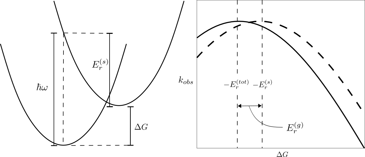
Figure 2: (Left) This schematic shows the relationship between the driving force $\Delta G$, the static reoganization energy $E_{r}^{(s)}$, and the vertical electronic excitation energy $\hbar\omega$. (Right) Expected inverted regime electron transfer rate curves highlighting the difference between the static reorganization energy $E_{r}^{(s)}$ (dashed) and the total reorganization energy $E_{r}^{(tot)}$ (solid). For the Hamiltonian in Eq. 1.6, the high temperature equilibrium electron transfer rate is given by Eq. 3.14 with $s(t)=0$ and where $E_{r}^{(tot)}>E_{r}^{(s)}$.

Three key features of the Hamiltonian were necessary for the above proof. The first is that the bath modes were purely harmonic. The second is that the modes maintained their respective frequencies when there was a change in electronic state. Third and finally, we relied on the fact that the initial state was a mixed state of vibrational eigenstates of one of the two system diabats (which allowed us to write Eq. 3.6). As mentioned in the introduction, this state of affairs suggests more distinct electron transfer rate effects may well emerge with either anharmonic bath models and/or nonequilibrium starting conditions.

3.2 Nonequilibrium dynamics

In order to treat the nonequilibrium case using the formalism from above, the only change we must make is to modify the initial density matrix. We will use the density matrix defined in Eq. 2.4. As shown in Appendix 7.3, the resulting autocorrelation function is:

$$C(t^{\prime},t^{\prime\prime}) =\text{Tr}\left[e^{-\beta\hat{H}_{B}}e^{i\sum_{\alpha}d_{\alpha}\hat{p}_{\alpha}}e^{i\sum_{\alpha}\lambda_{\alpha}\hat{p}_{\alpha}(t^{\prime\prime})+W_{\alpha}\hat{x}_{\alpha}(t^{\prime\prime})}e^{-i\sum_{\alpha}\lambda_{\alpha}\hat{p}_{\alpha}(t^{\prime})+W_{\alpha}\hat{x}_{\alpha}(t^{\prime})}e^{-i\sum_{\alpha}d_{\alpha}\hat{p}_{\alpha}}\right]$$ (3.11)

$$=e^{-\sum_{\alpha}(\overline{\lambda}_{\alpha}^{2}+\overline{W}_{\alpha}^{2})\left[2n_{\alpha}+1-(n_{\alpha}+1)e^{-i\omega_{\alpha}(t^{\prime\prime}-t^{\prime})}-n_{\alpha}e^{i\omega_{\alpha}(t^{\prime\prime}-t^{\prime})}\right]}\;\;\times$$

$$\qquad e^{\sum_{\alpha}\left(\overline{\lambda}_{\alpha}-i\overline{W}_{\alpha}\right)\left(e^{-i\omega_{\alpha}t^{\prime\prime}}-e^{-i\omega_{\alpha}t^{\prime}}\right)\overline{d}_{\alpha}-\left(\overline{\lambda}_{\alpha}+i\overline{W}_{\alpha}\right)\left(e^{i\omega_{\alpha}t^{\prime\prime}}-e^{i\omega_{\alpha}t^{\prime}}\right)\overline{d}_{\alpha}}$$ (3.12)

$$\qquad\overline{\lambda}_{\alpha}=\lambda_{\alpha}\sqrt{\frac{m_{\alpha}\omega_{\alpha}}{2}}\qquad\overline{W}_{\alpha}=\frac{W_{\alpha}}{\sqrt{2m_{\alpha}\omega_{\alpha}}}\qquad\overline{d}_{\alpha}=d_{\alpha}\sqrt{\frac{m_{\alpha}\omega_{\alpha}}{2}}$$

Substituting this expression into the integral in Eq. 2.1, we obtain a general first-order population expression:

$$\begin{split}P_{2}(t)\simeq\lvert V\rvert^{2}\int_{0}^{t}dt^{\prime}\,\int_{0}^{t}dt^{\prime\prime}\,e^{-i(E_{2}-E_{1})(t^{\prime\prime}-t^{\prime})}e^{-\sum_{\alpha}(\overline{\lambda}_{\alpha}^{2}+\overline{W}_{\alpha}^{2})\left[2n_{\alpha}+1-(n_{\alpha}+1)e^{-i\omega_{\alpha}(t^{\prime\prime}-t^{\prime})}-n_{\alpha}e^{i\omega_{\alpha}(t^{\prime\prime}-t^{\prime})}\right]}\;\;\times\\ \qquad e^{\sum_{\alpha}\left(\overline{\lambda}_{\alpha}-i\overline{W}_{\alpha}\right)\left(e^{-i\omega_{\alpha}t^{\prime\prime}}-e^{-i\omega_{\alpha}t^{\prime}}\right)\overline{d}_{\alpha}-\left(\overline{\lambda}_{\alpha}+i\overline{W}_{\alpha}\right)\left(e^{i\omega_{\alpha}t^{\prime\prime}}-e^{i\omega_{\alpha}t^{\prime}}\right)\overline{d}_{\alpha}}\end{split}$$ (3.13)

Here, $P_{2}(t)$ describes the gradual development of population in state $\lvert 2\rangle$ starting with $P_{2}(0)=0$. One can take the time derivative of the equation above and obtain a time-dependent rate of transition from the $\lvert 1\rangle$ state to the $\lvert 2\rangle$ state. The formal (time dependent) rate constant is given in Eq. 7.24. In the high-temperature Markovian limit, the rate expression can be explicitly evaluated, producing a time-dependent golden rule rate expression of the form:

$$k(t)=\frac{2\pi\lvert V\rvert^{2}}{\sqrt{4\pi E_{r}^{(tot)}k_{B}T}}\text{exp}\left(-\frac{(\Delta G^{\circ}+E_{r}^{(tot)}+s(t))^{2}}{4E_{r}^{(tot)}k_{B}T}\right)$$ (3.14)

$$s(t)=\sum_{\alpha}d_{\alpha}\left[m_{\alpha}\omega_{\alpha}^{2}\lambda_{\alpha}\cos(\omega_{\alpha}t)-W_{\alpha}\omega_{\alpha}\sin(\omega_{\alpha}t)\right]$$ (3.15)

where $E_{r}^{(tot)}$ is the total reorganization energy that arises due to the combined effects of $E_{r}^{(s)}$ and $E_{r}^{(g)}$. Note that Eq. 3.14 for the time-dependent rate constant has a form that is very similar to that of a classical Marcus theory time-independent rate expression. In this high temperature limit, the dressed reorganization energy $E_{r}^{(tot)}$ and dephasing function $s(t)$ are enough to fully characterize the nonequilibrium rate dynamics. These parameters are in turn characterized by the bath density of modes, as well as the shift parameters $\lambda_{\alpha}$, $d_{\alpha}$, and $W_{\alpha}$. The physical meaning of each of these terms is summarized in Table 1 and Figure 3 as a reminder to the reader.

Parameter	Physical Meaning
$s(t)$	Dephasing function for nonequilibrium fluctuations
$d_{\alpha}$	Shift of initial bath states away from equilibrium
$W_{\alpha}$	Spatial frequency of the phase oscillations of the interstate coupling
$\lambda_{\alpha}$	Physical shift between diabatic potential wells

Table 1: The key parameters that define the rate of nonequilibrium relaxation.

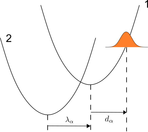
Figure 3: The physical meaning of the terms $\lambda_{\alpha}$ and $d_{\alpha}$.

Let us now focus on the dephasing function $s(t)$ in Eq. 3.15. This function contains all information regarding the transient behavior of the system, serving to capture the fluctuations in the interstate energy gap as the nuclear geometry evolves. Note in particular that the second term in $s(t)$ changes when any single $W_{\alpha}$ changes sign, clearly indicating a spin-dependent rate effect. Additionally, in the case that the number of modes in the bath is very large, $s(t)$ tends to 0 as $t$ grows large, implying that the system tends to equilibrium dynamics. Therefore, $s(t)$ indeed contains information about the dephasing of the bath. As the bath dephases and returns to equilibrium, we expect, based on the result from section 3.1, that all Berry force effects should be damped out.

Before concluding this section and presenting our results, let us note that, in order to simulate photoexcitation in a two-state system, one can simply set $d_{\alpha}=-\lambda_{\alpha}$ for all $\alpha$ (see Fig. 3), and such a choice will manifest itself directly in the dynamics of the dephasing function in Eq. 3.15. Note, however, that the present model can also be applied to systems where the final acceptor state is not the same as the ground state, such as multistate models and/or intersystem crossings. In such cases, to retain full generality, one must not assume $d_{\alpha}=-\lambda_{\alpha}$.

4 Results

4.1 Photoexcitation dynamics in a continuum bath model

In a typical analysis of a spin-boson system (i.e. in the Condon approximation), one assumes that the system-bath interaction can be characterized by a spectral density. Working from such an approximation, one can compute the reorganization energy, which fully characterizes relaxation dynamics. However, in the model we have investigated thus far, a single spectral density is insufficient to characterize the system-bath interaction; the system exchanges energy through both the system-bath coupling and spin-orbit effects so that we must fix two sets of parameters, $\lambda_{\alpha}$ and $W_{\alpha}$.

To make such parameterization as simple as possible, we will assume a density of modes $\rho(\omega)=(\eta\omega/\omega_{C}^{2})\exp(-\omega/\omega_{C})$. $\omega_{C}$ describes a cutoff frequency for the bath and $\eta$ is a normalization factor that ensures integration over the density function returns the correct number of modes in the bath. For the diabats, we will then further assume that the mass-weighted shifts between the two surfaces are uniform across all modes, i.e. $\lambda_{\alpha}\sqrt{m_{\alpha}}=\lambda$ for all $\alpha$. Similarly, we set $W_{\alpha}/\sqrt{m_{\alpha}}$ equal to a constant $W$ for all $\alpha$. Note that $W$ can be positive or negative. For the bath displacement parameters $d_{\alpha}$, we set the mass weighted displacements $d_{\alpha}\sqrt{m_{\alpha}}$ equal to $-\kappa\lambda$. As discussed earlier, $\kappa=1$ corresponds to relaxation of a photoexcited system.

In order to characterize the dynamics, we need to compute the reorganization energy and the dephasing function. We begin with the reorganization energy. The total reorganization energy is the sum over all modes of the single-mode reorganization energies:

$$E_{r}^{(tot)} =\sum_{\alpha}\frac{1}{2}m_{\alpha}\omega_{\alpha}^{2}\lambda_{\alpha}^{2}+\frac{W_{\alpha}^{2}}{2m_{\alpha}}$$

$$=\frac{1}{2}\int_{0}^{\infty}d\omega\,\rho(\omega)(\omega^{2}\lambda^{2}+W^{2})$$

$$=3\eta\omega_{C}^{2}\lambda^{2}+\frac{\eta}{2}W^{2}$$ (4.1)

Below, it will sometimes be helpful to switch variables from $(\lambda,W)$ to $(E_{r}^{(tot)},\theta)$:

$$\lambda=\sqrt{\frac{E_{r}^{(tot)}}{3\eta\omega_{C}^{2}}}\cos\theta\qquad W=\sqrt{\frac{2E_{r}^{(tot)}}{\eta}}\sin\theta$$ (4.2)

Next, we calculate the dephasing function $s(t)$:

$$s(t) =\sum_{\alpha}d_{\alpha}\left[m_{\alpha}\omega_{\alpha}^{2}\lambda_{\alpha}\cos(\omega_{\alpha}t)-W_{\alpha}\omega_{\alpha}\sin(\omega_{\alpha}t)\right]$$

$$=-\kappa\int_{0}^{\infty}d\omega\,\rho(\omega)\left(\omega^{2}\lambda^{2}\cos(\omega t)-\omega\lambda W\sin(\omega t)\right)$$

$$=-\kappa\left[\frac{6\eta\lambda^{2}\omega_{C}^{2}\left(\omega_{C}^{4}t^{4}-6\omega_{C}^{2}t^{2}+1\right)}{\left(\omega_{C}^{2}t^{2}+1\right)^{4}}+\frac{2\eta\lambda W\omega_{C}\left(\omega_{C}^{3}t^{3}-3\omega_{C}t\right)}{\left(\omega_{C}^{2}t^{2}+1\right)^{3}}\right]$$ (4.3)

In terms of $E_{r}^{(tot)}$ and $\theta$, the dephasing function is:

$$\begin{split}s(t)=-\frac{\kappa E_{r}^{(tot)}}{(\omega_{C}^{2}t^{2}+1)^{4}}\Big{[}(1+\cos 2\theta)(\omega_{C}^{4}t^{4}-6\omega_{C}^{2}t^{2}+1)+\\ \sqrt{\frac{2}{3}}\sin 2\theta(\omega_{C}^{5}t^{5}-2\omega_{C}^{3}t^{3}-3\omega_{C}t)\Big{]}\end{split}$$ (4.4)

In Fig. 4, we show rate constants and population yields that were calculated for a photogenerated ($\kappa=1$) distribution using the high-temperature expression, Eqn. 3.14. We fix the static reorganization energy $E_{r}^{(s)}$ and add in some amount of geometric reorganization energy ($E_{r}^{(g)}=\frac{W^{2}}{2m}$); the ratio is quantified by $\theta$ in Eq. 4.2. In subplot (a), we plot the population for short and long times for different values of $\theta$. At long times, as expected, we see the dynamics for $\pm\theta$ gradually approach the same equilibrium rate as time progresses. Here, we emphasize that the disagreement between the exact NEFGR expression and the high temperature expression for $\theta=\pm 0.5$ is not the result of any interesting dynamical effect that depends on $\theta$. Instead, a simple numerical calculation shows that the exact and high temperature expressions differ simply because of tunneling effects (whose importance depends on the total value of the reorganization energy $E_{r}^{(tot)}$). Note that $E_{r}^{(tot)(\theta=0.5)}=E_{r}^{(tot)(\theta=-0.5)}\neq E_{r}^{(tot)(\theta=0)}$

The more interesting behavior occurs at short times while the bath still has yet to decohere and where the population curves can depend sensitively on $\pm\theta$ (i.e. $\pm W$). To see these dynamics clearly, we zoom in within subfigures $(b)$ and $(c)$. Here, we find transient populations for $\theta=-0.5$ that are 50% larger than those of $\theta=0.5$. In general, Berry force effects are larger when we calculate populations with the exact (rather than the high temperature) expression, but overall, the high temperature expression clearly reflects the correct qualitative physics (especially if we compare only $\theta$ with $-\theta$ data).

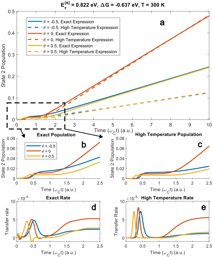
Figure 4: A comparison between the dynamics computed numerically using the exact Fermi Golden Rule expression and those derived from the high temperature expression for $\theta=0,0.5,-0.5$. We plot the population on state 2 $(P_{2}$) as a function of time. $\omega_{C}$ is taken to be 0.001 a.u. For long times, the populations and rate expressions all converge to the equilibrium data, so that $P_{2}(\theta=0.5)=P_{2}(\theta=-0.5)$. At short times, however, as emphasized by subfigures $(b)-(e)$, the dynamics for $\pm\theta$, i.e. $\pm W$, can be very difficult and exhibit strong Berry force effects. Note that results computed using the high-temperature expression qualitatively capture features of those computed with the exact FGR expression, especially at short times, tracking well the relative timing and magnitude of the transient rate spikes.

Lastly, in subfigures $(d)$ and $(e)$, we plot the derivative of the population data, i.e. the instantaneous rates. Here, we can clearly see differences in the features of the early time dynamics, including the magnitude and the relative timing of the populations spikes. Again, we find that the high temperature approximation is a reasonably good approximation for the exact early time dynamics (and computationally cheaper to evaluate).

Finally, and most importantly, we would like to ask whether any rate differences between systems with opposite signs ($\pm W$) can persist for a significant period of time. In order to probe this question for a wide variety of $\theta$ values (while avoiding excessive computational expense), we will use the high-temperature expression above. We can roughly quantify dynamical differences by focusing on rate dynamics at the time $1/\omega_{C}$, i.e. the characteristic dephasing time of the bath. For this data set, we will fix the total reorganization energy $E_{r}^{(tot)}$; if we were to fix $E_{r}^{(s)}$ as before, the variation in $E_{r}^{(tot)}$ would be very large and make it difficult to isolate effects arising from the geometric component. (Moreover, as noted above in Fig. 4, the quantitative accuracy of the high-temperature approximation depends on the total value of $E_{r}^{(tot)}$ and whether one can safely ignore tunneling; by fixing $E_{r}^{(tot)}$, we can thus reasonably assume a cancellation of error and compare the effect of exchanging $E_{r}^{(g)}$ with $E_{r}^{(s)}$).

Our results are plotted in Fig. 5. We consider two related quantities. First, we plot the spin polarization at time $1/\omega_{C}$:

$$\frac{k_{+}-k_{-}}{k_{+}+k_{-}}$$ (4.5)

where $k(t)$ is as defined in Eq. 3.14 and $k_{-}$ is related to $k_{+}$ through a change in sign on the $\{W_{\alpha}\}$ terms. As shown in Fig. 5, the polarization can become quite large, reaching nearly 60 percent in photoexcitation processes in the 200 to 400 K range. Note the antisymmetry in the polarization plot across the line $\theta=0$. This antisymmetry arises naturally because changing the sign of $\theta$ corresponds to changing the signs on the $\{W_{\alpha}\}$ terms (which results in opposite spin polarization).

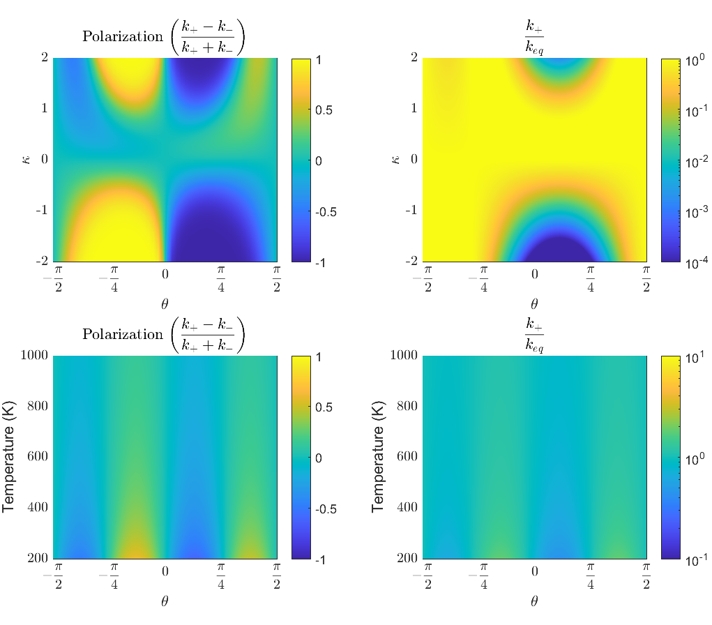
Figure 5: (Left) Comparison of the spin polarization (see Eq. 4.5) at time $1/\omega_{C}$ after initiation of dynamics for a range of values of $\kappa$, $\theta$, and temperature. Depending on the fraction of geometric vs. standard reorganization energy, one can find a great deal of spin polarization if one starts far from equilibrium (large $\kappa$) and if the temperature is not too large. (Right) Comparison of the rate dynamics at time $1/\omega_{C}$ relative to the final equilibrium rate (following bath dephasing) for a range of values of $\kappa$, $\theta$, and temperature. Berry forces can have large effects, with relative transient rates $\sim 10^{3}$ possible between different $\left\{W_{\alpha}\right\}$ and $\left\{-W_{\alpha}\right\}$ values (leading to spin polarization on the order of unity). Parameters: All plots have $E_{r}^{(tot)}=0.822$ eV and $\Delta G=-0.637$ eV. The upper plots were generated using a temperature of 300 K and the lower plots were generated for photoexcitations, i.e. $\kappa=1$. All data was generated in the high temperature approximation (see Eqs. 3.14 and 4.4).

Second, in Fig. 5, we also plot

$$\frac{k_{+}}{k_{eq}}$$ (4.6)

in order to quantify the absolute magnitude of the effect of the $\left\{W_{\alpha}\right\}$ terms. We find that the nonequilibrium rates with $W\neq 0$ can be very different from the rates with $W=0$, sometimes by as much as a factor of 1000 for systems prepared far from equilibrium. Interestingly, the rate at time $1/\omega_{C}$ is never significantly faster than the equilibrium rate; but there are certain regimes in which the transfer rate is much slower. This result suggests that the spin polarization observed is a result not of favoring one electronic spin, but rather disfavoring the other. Finally, we observe that as the temperature of the system is raised, polarization effects due to spin-orbit effects gradually disappear, reflecting the fact that geometric phase effects are highly dependent on bath coherences.

Although the high temperature expression is useful, it cannot provide a complete picture of the system behavior at low to intermediate temperatures. In Fig. 6, we plot the transient spin polarization as a function of temperature for $\theta=-0.5$ using the full NEFGR expression (not the high temperature expression). We find a more nuanced picture; the spin polarization does not increase monotonically as one lowers the temperature, but rather has a maximum at some intermediate temperature. Interestingly, such non-monotonic temperature dependence has also been observed (experimentally and theoretically) by Naaman, Fransson and co-workers in the context of spin polarization arising from conduction through DNA base pairs ⁴².

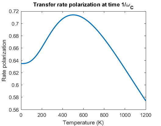
Figure 6: A visualization of the temperature dependence of the transient rate polarization (polarization at time $1/\omega_{C}$) for $\theta=-0.5$. Note that the polarization attains a maximum at an intermediate temperature and approaches a fixed limit as the temperature approaches 0. (Although the high-temperature expression correctly captures the asymptotic behavior, the decrease in polarization at lower temperatures can only be observed using the full NEFGR expression.) Parameters: $E_{r}^{(s)}$ = 0.822 eV, $\Delta G$ = -0.637 eV, $\theta$ = -0.5.

5 Discussion

From the results presented above, it is clear that Berry forces can survive nuclear friction and that spin-dependent electron transfer dynamics are indeed possible. Although spin-orbit coupling effects (i.e. the effects of the sign of $W$) vanish in equilibrium and contribute only a small amount to the total reorganization energy, these effects can be quite important for systems prepared far from equilibrium. At the same time, however, the present work only scratches the surface of how electronic spin ties into electron transfer, and opens up a slew of questions.

First, what is the most reasonable Hamiltonian that one should use when describing spin-dependent electron transfer? In the present manuscript, we have simply assumed an exponential complex-valued diabatic coupling that changes according to $e^{i\sum_{\alpha}W_{\alpha}\hat{x}_{\alpha}}$. Where does such a term come from? In principle, we expect an interstate coupling in the electronic Hamiltonian to be of the form:

$$a(\hat{x})+ib(\hat{x})=c(\hat{x})e^{id(\hat{x})}$$ (5.1)

where $a(\hat{x})$ is a standard, real-valued diabatic coupling and $ib(\hat{x})$ is the purely imaginary-valued spin -orbit coupling, as calculated in Appendix 7.1. Thus, the phase $d(\hat{x})$ must originate from a competition between different effects (e.g. the ratio between a position dependent spin-orbit coupling and a position independent diabatic coupling, or the ratio between a position dependent diabatic coupling and a position independent spin-orbit coupling). If one assumes $c(\hat{x})$ is a constant, and one expands $d(\hat{x})\approx\sum W_{\alpha}\hat{x}_{\alpha}$ as a Taylor series, one recovers the ESOC Hamiltonian in Eq. 1.6. At present, our group is expending a great deal of effort running ab initio calculations searching for systems where $|W|$ will be large and/or meaningful. One must wonder: how large can $|W|$ be in practice (especially if SOC is small), and is it reasonable to make the exponentiation in Eq. 5.1 over the relevant volume of configuration space where two diabatic curves cross?

Questions about the validity of the ESOC model can be addressed in the future by investigating alternative forms for the interstate coupling, for instance the more common Linear Vibronic Coupling (LVC) type model^{40, 43, 36}. In the LVC model, the interstate coupling is taken to be linear in position for all bath modes, i.e. $\hat{V}=\sum_{\alpha}c_{\alpha}\hat{x}_{\alpha}\lvert 1\rangle\langle 2\rvert+c^{*}_{\alpha}\hat{x}_{\alpha}\lvert 2\rangle\langle 1\rvert$. The LVC model is standard for investigating dynamics of systems around conical intersections, but this model must also break down at some point because the off-diagonal couplings grow to infinity away from the origin. Nevertheless, if one works with an LVC (or an LVC-like model), a second question one can ask is: what dynamics do we observe when a conical intersection is broken by a small amount of spin-orbit coupling? Note that, within an LVC model, adding spin-orbit coupling will be completely different from adding a real-valued constant coupling (of equal magnitude); a real valued coupling would shift the LVC conical intersection, whereas an imaginary spin-orbit coupling would remove the conical intersection entirely (and lead to a large $W$). While such a removal might also not seem entirely realistic^{44, 45, 46}, this scenario makes clear that electron transfer effects may emerge that are wholly unique to strongly spin-dependent systems.

A third question relates to the displaced harmonic oscillator model for nuclear motion. Above, the equivalence of equilibrium dynamics for $\hat{H}$ and $\hat{H}^{*}$ arose almost accidentally and is clearly tied to the ESOC Hamiltonian. Although first-order FGR rates may be identical for $\hat{H}$ and $\hat{H}^{*}$ for all rate processes (see Eq. 1.5), there is no reason to expect (in general) that these equilibrium rates will be the same at second or higher order. For example, in Fig. 7 below, we plot dynamics for one single anharmonic mode, where dynamics are initialized in the lowest eigenstate of the upper diabat. Clearly, the dynamics show a small (but nonzero) spin dependence. In general, will these differences be small (because they show up only at higher orders of perturbation theory) or will these differences be significant (because they can add together for many anharmonic modes)? One must also be very curious about the dynamics of a model with Duschinskii rotations⁴⁷ – do such rotations (which introduce stronger directionality on the bath reorganization) amplify the effects of spin-dependent nuclear forces? One significant challenge will be to quantify the magnitude of spin-dependence for equilibrium dynamics in systems beyond the displaced oscillator approximation.

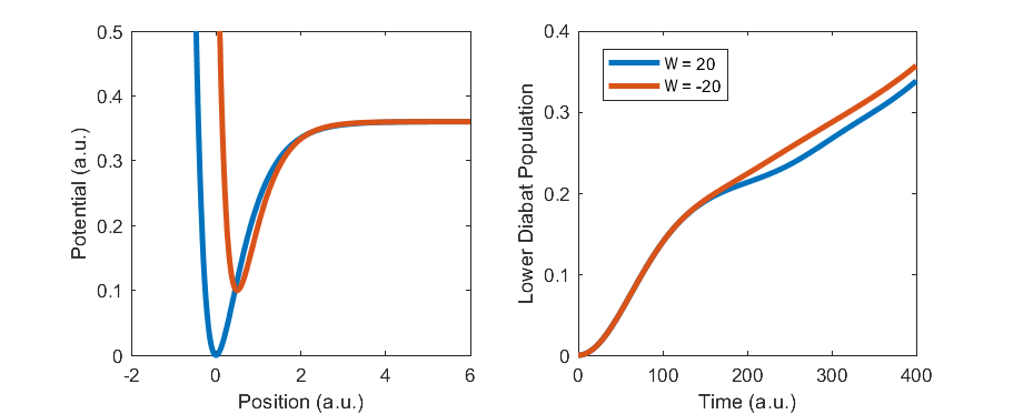
Figure 7: The Morse potential surfaces are parametrized such that they exhibit the same force constant in the harmonic approximation and the coupling between the surfaces is taken to be of the form $Ve^{iW\hat{x}}\lvert 1\rangle\langle 2\rvert+V^{*}e^{-iW\hat{x}}\lvert 2\rangle\langle 1\rvert$. The dynamics are initialized in the lowest eigenstate of the upper well. Note that the population dynamics for opposite signs on $W$ exhibit good agreement at very short time, but soon diverge, suggesting that higher order effects may be of great significance in anharmonic systems.

Finally, the goal of this research direction is to identify realistic systems that will display strong Berry force effects. Obviously, one would like to work with ab initio electronic structure Hamiltonians and run dynamics, but such a course of study is expensive. Even if, for a moment, we commit to studying model Hamiltonians, it is not wholly clear how to best map model dynamics to the real world. For instance, even though the standard spin-boson model has been used very successfully to model electron transfer over the years, it is clear that a more complicated parameter space of models will be necessary to discern Berry force effects. After all, within the ansatz of a two level system, Berry force arises by breaking the Condon-approximation, and so we must require not one, but two spectral densities; one of these spectral densities mediates energy exchange between the electronic and vibrational systems (as in the standard spin-boson model) and the other characterizes how the vibrational states mediate the spin-orbit coupling between electronic states. Do these interactions proceed with the same natural set of vibrational states? How should these spectra be tuned to one another in order to maximize spin-related electron transfer effects? Can we disentangle these effects in a meaningful way? Lastly, if we return to the question of electronic structure, one must ponder how best to map a realistic system to the model Hamiltonians discussed above: in particular, will we necessarily find that, within floppy molecular structures, metal ions with large spin-orbit couplings always experience bigger Berry force effects during an electronic transition, or are the dynamics more complicated? For instance, some recent experiments suggest that the CISS effect can be sensitive to an ion with strong spin-orbit coupling⁴⁸ while other experiments suggest that spin-orbit coupling in a substrate is not important to the overall CISS signal⁴⁹. If we can broadly answer such questions, we will clearly gain a great deal of intuition as far as rationally designing viable molecules and pathways with exciting new chemistry, and ideally gain the capacity to separate metal ions with large spin-orbit coupling from those with small spin-orbit coupling.

6 Conclusions

In conclusion, we have investigated a complex-valued spin-boson-like model Hamiltonian using nonequilibrium Fermi golden rule theory in order to provide fundamental insight into how spin-orbit coupling might influence condensed phase electron transfer. Our investigations have shown that Berry force effects can survive nuclear friction for some (measurable) period of time, before the effect dissipates. The exact details of how long such an effect survives is complicated and depends sensitively on the exact nuclear motion – the ESOC model presented here is simple to treat theoretically, but difficult to map to an ab intio Hamiltonian. Further research will be necessary to better quantify the effect and gain intuition as to exactly how big these Berry forces can be (and when) and if/how nuclear vibrations either correlate with or cause a CISS effect⁵⁰. Moreover, in the future, if we wish to run predictive simulations of realistic molecules with ab initio potentials, it will be necessary to develop efficient and inexpensive semiclassical algorithms^{17, 51, 52} for treating nuclear curve-crossing dynamics in the presence of spin orbit coupling.

7 Appendix

In this appendix, we briefly discuss the connection between electronic spin and complex Hamiltonians, and then proceed to derive some of the necessary equations presented above for the nonequilibrium golden rule calculations.

7.1 Spin-dependence due to the $\hat{\textbf{L}}\cdot\hat{\textbf{S}}$ operator

Consider a molecular system with two electronic states labeled $\lvert 1\rangle$ and $\lvert 2\rangle$ at a fixed geometry. In adding a spin-orbit effect, we must consider spin states $\lvert 1,\uparrow\rangle$, $\lvert 2,\uparrow\rangle$, $\lvert 1,\downarrow\rangle$, $\lvert 2,\downarrow\rangle$. In principle, we can write the Hamiltonian as a sum

$$\hat{H}=\hat{H}_{0}+\xi\,\hat{\textbf{L}}\cdot\hat{\textbf{S}}$$ (7.1)

where $\hat{H}_{0}$ is spin-independent and $\xi$ is the strength of the spin-orbit interaction. Since $\hat{H}_{0}$ is spin-independent, it can only couple states of identical spin. Therefore, in the spin-state basis, we can write $H_{0}$ as follows:

$$\hat{H}_{0}=\begin{pmatrix}E_{1}&0&V&0\\ 0&E_{1}&0&V\\ V&0&E_{2}&0\\ 0&V&0&E_{2}\end{pmatrix}\qquad\begin{pmatrix}\lvert 1,\uparrow\rangle\\ \lvert 1,\downarrow\rangle\\ \lvert 2,\uparrow\rangle\\ \lvert 2,\downarrow\rangle\end{pmatrix}$$ (7.2)

Now we construct the $\hat{\textbf{L}}\cdot\hat{\textbf{S}}$ matrix. We note that if $\lvert 1\rangle$ and $\lvert 2\rangle$ are molecular orbitals in an appropriate representation, they do not couple to themselves through any of the three component angular momentum operators. Thus, we can write the $\hat{\textbf{L}}\cdot\hat{\textbf{S}}$ matrix as follows:

$$\hat{\textbf{L}}\cdot\hat{\textbf{S}}=\begin{pmatrix}0&0&\langle 1|\hat{\textbf{L}}_{z}|2\rangle&\langle 1|\hat{\textbf{L}}_{x}-i\hat{\textbf{L}}_{y}|2\rangle\\ 0&0&\langle 1|\hat{\textbf{L}}_{x}+i\hat{\textbf{L}}_{y}|2\rangle&-\langle 1|\hat{\textbf{L}}_{z}|2\rangle\\ \langle 2|\hat{\textbf{L}}_{z}|1\rangle&\langle 2|\hat{\textbf{L}}_{x}-i\hat{\textbf{L}}_{y}|1\rangle&0&0\\ \langle 2|\hat{\textbf{L}}_{x}+i\hat{\textbf{L}}_{y}|1\rangle&-\langle 1|\hat{\textbf{L}}_{z}|2\rangle&0&0\end{pmatrix}$$ (7.3)

Noting that the angular momentum component operators are purely imaginary, we can write the matrix more concisely:

$$\hat{\textbf{L}}\cdot\hat{\textbf{S}}=\begin{pmatrix}0&0&\alpha&\beta\\ 0&0&-\beta^{*}&-\alpha\\ \alpha^{*}&-\beta&0&0\\ \beta^{*}&-\alpha^{*}&0&0\end{pmatrix}\qquad\begin{pmatrix}\lvert 1,\uparrow\rangle\\ \lvert 1,\downarrow\rangle\\ \lvert 2,\uparrow\rangle\\ \lvert 2,\downarrow\rangle\end{pmatrix}$$ (7.4)

Note that $\alpha$ is purely imaginary whereas $\beta$ has a real component, so the upper right block is anti-Hermitian and traceless. Therefore, this 2x2 matrix is diagonalizable and has purely imaginary eigenvalues $\alpha^{\prime}$ and $\alpha^{\prime*}=-\alpha^{\prime}$. The lower left block is just the conjugate transpose of the (anti-Hermitian) upper right block, and so is diagonalized by the same change of basis. Furthermore, the eigenvalues of the lower left block are conjugate to the eigenvalues of the upper right block. Note that a change of spin basis does not affect $\hat{H}_{0}$, which is block diagonal. We can now write down the total fixed-geometry Hamiltonian in the new spin basis (recall that $\xi$ is defined in Eq. 7.1):

$$\hat{H}=\begin{pmatrix}E_{1}&0&V&0\\ 0&E_{1}&0&V\\ V&0&E_{2}&0\\ 0&V&0&E_{2}\end{pmatrix}+\begin{pmatrix}0&0&\xi\cdot\alpha^{\prime}&0\\ 0&0&0&\xi\cdot\alpha^{\prime*}\\ \xi\cdot\alpha^{\prime*}&0&0&0\\ 0&\xi\cdot\alpha^{\prime}&0&0\end{pmatrix}\qquad\begin{pmatrix}\lvert 1,\uparrow^{\prime}\rangle\\ \lvert 1,\downarrow^{\prime}\rangle\\ \lvert 2,\uparrow^{\prime}\rangle\\ \lvert 2,\downarrow^{\prime}\rangle\end{pmatrix}$$ (7.5)

Therefore, at any nuclear geometry, the four-dimensional Hilbert space above (for spin-electronic wavefunctions with two spatial orbitals) can always be partitioned into two distinct subspaces, each with a distinct Hamiltonian $\hat{H}$ and $\hat{H}^{*}$ corresponding to one spin or the other opposite spin.

In this article, we have made the assumption that that such a partition will be valid and unchanged for all nuclear geometries. This strong assumption allows us to assume that we can entirely ignore all spin-flip processes.

7.2 Evaluation of Eq. 3.5

To evaluate Eq. 3.5, we begin with the polaronic Hamiltonian in 3.2, restated here:

$$\hat{H}=E_{1}\lvert 1\rangle\langle 1\rvert+E_{2}\lvert 2\rangle\langle 2\rvert+\hat{V}\lvert 1\rangle\langle 2\rvert+\hat{V}^{\dagger}\lvert 2\rangle\langle 1\rvert+\hat{H}_{B}$$

$$\hat{V}=Ve^{i\sum_{\alpha}\lambda_{\alpha}\hat{p}_{\alpha}+W_{\alpha}\hat{x}_{\alpha}}\qquad\lambda_{\alpha}=\frac{c_{\alpha}^{(1)}-c_{\alpha}^{(2)}}{m_{\alpha}\omega_{\alpha}^{2}}$$

We will use $\hat{\mathcal{R}}$ as defined in Eq. 3.4 to perform a unitary transformation on the polaronic Hamiltonian. We need to compute $\hat{\mathcal{R}}\hat{H}\hat{\mathcal{R}}^{\dagger}$. $\hat{\mathcal{R}}$ obviously commutes with $\hat{H}_{B}$. Thus, all we need to compute is $\hat{\mathcal{R}}e^{i\sum_{\alpha}W_{\alpha}\hat{x}_{\alpha}+\lambda_{\alpha}\hat{p}_{\alpha}}\hat{\mathcal{R}}^{\dagger}$. Using the fact that (for any operator $\hat{M}$)

$$e^{i\hat{H}t}e^{\hat{M}}e^{-i\hat{H}t}=e^{M(t)}$$ (7.6)

it follows that:

$$\hat{\mathcal{R}}e^{i\sum_{\alpha}W_{\alpha}\hat{x}_{\alpha}+\lambda_{\alpha}\hat{p}_{\alpha}}\hat{\mathcal{R}}^{\dagger}=\prod_{\alpha}e^{i\left(W_{\alpha}\hat{x}_{\alpha}(t)+\lambda_{\alpha}\hat{p}_{\alpha}(t)\right)}\Big{|}_{t=\arctan\left(\overline{W}_{\alpha}/\overline{\lambda}_{\alpha}\right)/\omega_{\alpha}}$$ (7.7)

$$\overline{\lambda}_{\alpha}=\lambda_{\alpha}\sqrt{\frac{m_{\alpha}\omega_{\alpha}}{2}}\qquad\overline{W}_{\alpha}=\frac{W_{\alpha}}{\sqrt{2m_{\alpha}\omega_{\alpha}}}$$

Keeping in mind that $t=\arctan\left(\overline{W}_{\alpha}/\overline{\lambda}_{\alpha}\right)/\omega_{\alpha}$, we find:

$$i\left(W_{\alpha}\hat{x}_{\alpha}(t)+\lambda_{\alpha}\hat{p}_{\alpha}(t)\right) =\overline{\lambda}_{\alpha}\left(ae^{-i\omega_{\alpha}t}-a^{\dagger}e^{i\omega_{\alpha}t}\right)+i\overline{W}_{\alpha}\left(ae^{-i\omega_{\alpha}t}+a^{\dagger}e^{i\omega_{\alpha}t}\right)$$ (7.8)

$$=\frac{\left(\overline{\lambda}_{\alpha}+i\overline{W}_{\alpha}\right)\left(\overline{\lambda}_{\alpha}-i\overline{W}_{\alpha}\right)}{\sqrt{\overline{\lambda}_{\alpha}^{2}+\overline{W}_{\alpha}^{2}}}a-\frac{\left(\overline{\lambda}_{\alpha}-i\overline{W}_{\alpha}\right)\left(\overline{\lambda}_{\alpha}+i\overline{W}_{\alpha}\right)}{\sqrt{\overline{\lambda}_{\alpha}^{2}+\overline{W}_{\alpha}^{2}}}a^{\dagger}$$ (7.9)

$$=i\left(\sqrt{\frac{2\left(\overline{\lambda}_{\alpha}^{2}+\overline{W}_{\alpha}^{2}\right)}{m_{\alpha}\omega_{\alpha}}}\right)\hat{p}_{\alpha}=i\left(\sqrt{\lambda_{\alpha}^{2}+\frac{W_{\alpha}^{2}}{m_{\alpha}^{2}\omega_{\alpha}^{2}}}\right)\hat{p}_{\alpha}=i\Gamma_{\alpha}\hat{p}_{\alpha}$$ (7.10)

Therefore, we conclude that

$$\hat{\mathcal{R}}\hat{H}\hat{\mathcal{R}}^{\dagger}=E_{1}\lvert 1\rangle\langle 1\rvert+E_{2}\lvert 2\rangle\langle 2\rvert+Ve^{i\sum_{\alpha}\Gamma_{\alpha}\hat{p}_{\alpha}}\lvert 1\rangle\langle 2\rvert+V^{*}e^{-i\sum_{\alpha}\Gamma_{\alpha}\hat{p}_{\alpha}}\lvert 2\rangle\langle 1\rvert+\hat{H}_{B}$$ (7.11)

7.3 Derivation of Eq. 3.13

In order to derive Eq. 3.13, we will work in the polaron representation of the ESOC Hamiltonian, as described above. We write the Hamiltonian as

$$\hat{H}=\hat{H}_{0}+\hat{V}$$ (7.12)

$$\hat{H}_{0}=E_{1}\lvert 1\rangle\langle 1\rvert+E_{2}\lvert 2\rangle\langle 2\rvert+\hat{H}_{B}$$ (7.13)

$$\hat{V}=Ve^{i\sum_{\alpha}\lambda_{\alpha}\hat{p}_{\alpha}+W_{\alpha}\hat{x}_{\alpha}}\lvert 1\rangle\langle 2\rvert+V^{*}e^{-i\sum_{\alpha}\lambda_{\alpha}\hat{p}_{\alpha}+W_{\alpha}\hat{x}_{\alpha}}\lvert 2\rangle\langle 1\rvert$$ (7.14)

Beginning with the density matrix $\hat{\rho}(0)$ in (2.4), We would like to approximate

$$\sum_{\textbf{v}^{\prime}}\langle 2,\textbf{v}^{\prime}|\rho(t)|2,\textbf{v}^{\prime}\rangle =\sum_{\textbf{v}^{\prime}}\sum_{\textbf{v}}\langle 2,\textbf{v}^{\prime}|e^{-i\hat{H}t}e^{-i\sum_{\alpha}d_{\alpha}\hat{p}_{\alpha}}e^{-\beta\hat{H}_{B}}|1,\textbf{v}\rangle\langle 1,\textbf{v}|e^{i\sum_{\alpha}d_{\alpha}\hat{p}_{\alpha}}e^{i\hat{H}t}|2,\textbf{v}^{\prime}\rangle$$ (7.15)

$$=\sum_{\textbf{v}}\langle 1,\textbf{v}|e^{i\sum_{\alpha}d_{\alpha}\hat{p}_{\alpha}}e^{i\hat{H}t}|2\rangle\langle 2|e^{-i\hat{H}t}e^{-i\sum_{\alpha}d_{\alpha}\hat{p}_{\alpha}}e^{-\beta\hat{H}_{B}}|1,\textbf{v}\rangle$$ (7.16)

$$=\text{Tr}_{B}\left[\langle 1|e^{i\sum_{\alpha}d_{\alpha}\hat{p}_{\alpha}}e^{i\hat{H}t}|2\rangle\langle 2|e^{-i\hat{H}t}e^{-i\sum_{\alpha}d_{\alpha}\hat{p}_{\alpha}}|1\rangle e^{-\beta\hat{H}_{B}}\right]$$ (7.17)

$$=\text{Tr}_{B}\left[e^{i\sum_{\alpha}d_{\alpha}\hat{p}_{\alpha}}\langle 1|e^{i\hat{H}t}|2\rangle\langle 2|e^{-i\hat{H}t}|1\rangle e^{-i\sum_{\alpha}d_{\alpha}\hat{p}_{\alpha}}e^{-\beta\hat{H}_{B}}\right]$$ (7.18)

Using the definitions $\hat{H}_{0}$ and $\hat{V}$ from above, we expand $\exp(-i\hat{H}t)$ to first order in a Dyson series as follows (I is the identity operator):

$$\left\langle 2\middle|e^{-i\hat{H}t}\middle|1\right\rangle \simeq\left\langle 2\middle|\textbf{I}-i\int_{0}^{t}dt^{\prime}\,e^{i\hat{H}_{0}t^{\prime}}\hat{V}e^{-i\hat{H}_{0}t^{\prime}}\middle|1\right\rangle$$

$$=-iV^{*}\int_{0}^{t}dt^{\prime}\,e^{i(E_{2}-E_{1})t^{\prime}}e^{i\hat{H}_{B}t^{\prime}}e^{-i\sum_{\alpha}\lambda_{\alpha}\hat{p}_{\alpha}+W_{\alpha}\hat{x}_{\alpha}}e^{-i\hat{H}_{B}t^{\prime}}$$ (7.19)

Now, we substitute this expression for $\left\langle 2\middle|e^{-i\hat{H}t}\middle|1\right\rangle$ (as well as the Hermitian transpose $\left\langle 1\middle|e^{i\hat{H}t}\middle|2\right\rangle$) into Eq. 7.18. Recognizing that $\text{Tr}_{B}\left[\exp(-\beta\hat{H}_{B})\hat{A}\right]=\left\langle\hat{A}\right\rangle$ for an operator $\hat{A}$, we find that (in the end), the population becomes a double integral with a time correlation function that must be evaluated:

$$\sum_{\textbf{v}^{\prime}}\langle 2,\textbf{v}^{\prime}|\rho(t)|2,\textbf{v}^{\prime}\rangle\simeq\lvert V\rvert^{2}\int_{0}^{t}dt^{\prime}\,\int_{0}^{t}dt^{\prime\prime}\,e^{-i(E_{2}-E_{1})(t^{\prime\prime}-t^{\prime})}C(t^{\prime},t^{\prime\prime})$$ (7.20)

$$C(t^{\prime},t^{\prime\prime})=\Big{\langle}e^{i\sum_{\alpha}d_{\alpha}\hat{p}_{\alpha}}e^{i\sum_{\alpha}\lambda_{\alpha}\hat{p}_{\alpha}(t^{\prime\prime})+W_{\alpha}\hat{x}_{\alpha}(t^{\prime\prime})}e^{-i\sum_{\alpha}\lambda_{\alpha}\hat{p}_{\alpha}(t^{\prime})+W_{\alpha}\hat{x}_{\alpha}(t^{\prime})}e^{-i\sum_{\alpha}d_{\alpha}\hat{p}_{\alpha}}\Big{\rangle}$$ (7.21)

In order to evaluate the time correlation function in the integrand, it is a relatively straightforward application of two operator identities:

$$e^{\hat{A}}e^{\hat{B}}=e^{\hat{A}+\hat{B}+\frac{1}{2}\left[\hat{A},\hat{B}\right]}\qquad\left\langle e^{\hat{A}}\right\rangle=e^{\frac{1}{2}\left\langle\hat{A}^{2}\right\rangle}$$

These relations are valid for operators $\hat{A}$ and $\hat{B}$ that linear in the position and momentum operators, which is the case for the product operator in the expectation value above.

As before, we use the following reduced forms for the coupling and shift coordinates:

$$\overline{\lambda}_{\alpha}=\lambda_{\alpha}\sqrt{\frac{m_{\alpha}\omega_{\alpha}}{2}}\qquad\overline{d}_{\alpha}=d_{\alpha}\sqrt{\frac{m_{\alpha}\omega_{\alpha}}{2}}\qquad\overline{W}_{\alpha}=\frac{W_{\alpha}}{\sqrt{2m_{\alpha}\omega_{\alpha}}}$$

We apply the first identity repeatedly to obtain

$$C(t^{\prime},t^{\prime\prime})=e^{\sum_{\alpha}\left(\overline{\lambda}_{\alpha}-i\overline{W}_{\alpha}\right)\left(e^{-i\omega_{\alpha}t^{\prime\prime}}-e^{-i\omega_{\alpha}t^{\prime}}\right)\overline{d}_{\alpha}-\left(\overline{\lambda}_{\alpha}+i\overline{W}_{\alpha}\right)\left(e^{i\omega_{\alpha}t^{\prime\prime}}-e^{i\omega_{\alpha}t^{\prime}}\right)\overline{d}_{\alpha}}\times$$

$$e^{-\frac{1}{2}\sum_{\alpha}\left(\overline{\lambda}_{\alpha}^{2}+\overline{W}_{\alpha}^{2}\right)\left(e^{i\omega_{\alpha}(t^{\prime\prime}-t^{\prime})}-e^{-i\omega_{\alpha}(t^{\prime\prime}-t^{\prime})}\right)}\Big{\langle}e^{\sum_{\alpha}\left(\overline{\lambda}_{\alpha}+i\overline{W}_{\alpha}\right)\left(e^{i\omega_{\alpha}t^{\prime\prime}}-e^{i\omega_{\alpha}t^{\prime}}\right)a_{\alpha}^{\dagger}-\left(\overline{\lambda}_{\alpha}-i\overline{W}_{\alpha}\right)\left(e^{-i\omega_{\alpha}t^{\prime\prime}}-e^{-i\omega_{\alpha}t^{\prime}}\right)a_{\alpha}}\Big{\rangle}$$ (7.22)

Finally, we apply the second identity to obtain the desired result:

$$C(t^{\prime},t^{\prime\prime})= e^{-\sum_{\alpha}(\overline{\lambda}_{\alpha}^{2}+\overline{W}_{\alpha}^{2})\left[2n_{\alpha}+1-(n_{\alpha}+1)e^{-i\omega_{\alpha}(t^{\prime\prime}-t^{\prime})}-n_{\alpha}e^{i\omega_{\alpha}(t^{\prime\prime}-t^{\prime})}\right]}\times$$

$$\qquad e^{\sum_{\alpha}\left(\overline{\lambda}_{\alpha}-i\overline{W}_{\alpha}\right)\left(e^{-i\omega_{\alpha}t^{\prime\prime}}-e^{-i\omega_{\alpha}t^{\prime}}\right)\overline{d}_{\alpha}-\left(\overline{\lambda}_{\alpha}+i\overline{W}_{\alpha}\right)\left(e^{i\omega_{\alpha}t^{\prime\prime}}-e^{i\omega_{\alpha}t^{\prime}}\right)\overline{d}_{\alpha}}$$ (7.23)

7.4 The High-Temperature Rate: Derivation of Eq. 3.14

To get a time-dependent rate expression, we take the time derivative of the double integral describing the 2-state population:

$$\frac{\partial}{\partial t}\lvert V\rvert^{2}\int_{0}^{t}dt^{\prime}\,\int_{0}^{t}dt^{\prime\prime}\,e^{-i(E_{2}-E_{1})(t^{\prime\prime}-t^{\prime})}C(t^{\prime},t^{\prime\prime})= \lvert V\rvert^{2}\int_{0}^{t}dt^{\prime\prime}\,e^{-i(E_{2}-E_{1})(t-t^{\prime})}C(t^{\prime},t)+$$

$$\lvert V\rvert^{2}\int_{0}^{t}dt^{\prime}\,e^{-i(E_{2}-E_{1})(t^{\prime\prime}-t)}C(t,t^{\prime\prime})$$ (7.24)

We begin by focusing on the first integral in Eq. 7.24:

$$\lvert V\rvert^{2}\int_{0}^{t}dt^{\prime\prime}\,e^{-i(E_{2}-E_{1})(t^{\prime\prime}-t)} e^{-\sum_{\alpha}(\overline{\lambda}_{\alpha}^{2}+\overline{W}_{\alpha}^{2})\left[2n_{\alpha}+1-(n_{\alpha}+1)e^{-i\omega_{\alpha}(t^{\prime\prime}-t)}-n_{\alpha}e^{i\omega_{\alpha}(t^{\prime\prime}-t)}\right]}\times$$

$$e^{\sum_{\alpha}\left(\overline{\lambda}_{\alpha}-i\overline{W}_{\alpha}\right)\left(e^{-i\omega_{\alpha}t^{\prime\prime}}-e^{-i\omega_{\alpha}t}\right)\overline{d}_{\alpha}-\left(\overline{\lambda}_{\alpha}+i\overline{W}_{\alpha}\right)\left(e^{i\omega_{\alpha}t^{\prime\prime}}-e^{i\omega_{\alpha}t}\right)\overline{d}_{\alpha}}$$ (7.25)

$$=\lvert V\rvert^{2}\int_{0}^{t}dt^{\prime\prime}\,e^{-i(E_{2}-E_{1})(t^{\prime\prime}-t)} e^{-\sum_{\alpha}(\overline{\lambda}_{\alpha}^{2}+\overline{W}_{\alpha}^{2})\left[2n_{\alpha}+1-(n_{\alpha}+1)e^{-i\omega_{\alpha}(t^{\prime\prime}-t)}-n_{\alpha}e^{i\omega_{\alpha}(t^{\prime\prime}-t)}\right]}\times$$

$$e^{\sum_{\alpha}\left(\overline{\lambda}_{\alpha}-i\overline{W}_{\alpha}\right)e^{-i\omega_{\alpha}t}\left(e^{-i\omega_{\alpha}(t^{\prime\prime}-t)}-1\right)\overline{d}_{\alpha}-\left(\overline{\lambda}_{\alpha}+i\overline{W}_{\alpha}\right)e^{i\omega_{\alpha}t}\left(e^{i\omega_{\alpha}(t^{\prime\prime}-t)}-1\right)\overline{d}_{\alpha}}$$ (7.26)

$$=\lvert V\rvert^{2}\int_{-t}^{0}d\tau\,e^{-i(E_{2}-E_{1})\tau} e^{-\sum_{\alpha}(\overline{\lambda}_{\alpha}^{2}+\overline{W}_{\alpha}^{2})\left[2n_{\alpha}+1-(n_{\alpha}+1)e^{-i\omega_{\alpha}\tau}-n_{\alpha}e^{i\omega_{\alpha}\tau}\right]}\times$$

$$e^{\sum_{\alpha}\left(\overline{\lambda}_{\alpha}-i\overline{W}_{\alpha}\right)e^{-i\omega_{\alpha}t}\left(e^{-i\omega_{\alpha}\tau}-1\right)\overline{d}_{\alpha}-\left(\overline{\lambda}_{\alpha}+i\overline{W}_{\alpha}\right)e^{i\omega_{\alpha}t}\left(e^{i\omega_{\alpha}\tau}-1\right)\overline{d}_{\alpha}}$$ (7.27)

In the high temperature limit, the second term in the integral decays quickly and we can use small-$\tau$ approximations. Therefore, we can approximate the integral as

$$\lvert V\rvert^{2}\int_{-t}^{0}d\tau\,e^{-i(E_{2}-E_{1})\tau} e^{-\sum_{\alpha}(\overline{\lambda}_{\alpha}^{2}+\overline{W}_{\alpha}^{2})\left[2n_{\alpha}+1-(n_{\alpha}+1)e^{-i\omega_{\alpha}\tau}-n_{\alpha}e^{i\omega_{\alpha}\tau}\right]}\times$$

$$e^{-\sum_{\alpha}\left(\overline{\lambda}_{\alpha}-i\overline{W}_{\alpha}\right)e^{-i\omega_{\alpha}t}\left(i\omega_{\alpha}\tau\right)\overline{d}_{\alpha}+\left(\overline{\lambda}_{\alpha}+i\overline{W}_{\alpha}\right)e^{i\omega_{\alpha}t}\left(i\omega_{\alpha}\tau\right)\overline{d}_{\alpha}}$$ (7.28)

$$=\lvert V\rvert^{2}\int_{-t}^{0}d\tau\,e^{-i(E_{2}-E_{1})\tau} e^{-\sum_{\alpha}(\overline{\lambda}_{\alpha}^{2}+\overline{W}_{\alpha}^{2})\left[2n_{\alpha}+1-(n_{\alpha}+1)e^{-i\omega_{\alpha}\tau}-n_{\alpha}e^{i\omega_{\alpha}\tau}\right]}\times$$

$$e^{-\sum_{\alpha}2i\omega_{\alpha}\overline{d}_{\alpha}\left[\overline{\lambda}_{\alpha}\cos(\omega_{\alpha}t)-\overline{W}_{\alpha}\sin(\omega_{\alpha}t)\right]\tau}$$ (7.29)

Next, we address the second integral in Eq. 7.24:

$$\lvert V\rvert^{2}\int_{0}^{t}d\tau\,e^{-i(E_{2}-E_{1})\tau} e^{-\sum_{\alpha}(\overline{\lambda}_{\alpha}^{2}+\overline{W}_{\alpha}^{2})\left[2n_{\alpha}+1-(n_{\alpha}+1)e^{-i\omega_{\alpha}\tau}-n_{\alpha}e^{i\omega_{\alpha}\tau}\right]}\times$$

$$e^{-\sum_{\alpha}2i\omega_{\alpha}\overline{d}_{\alpha}\left[\overline{\lambda}_{\alpha}\cos(\omega_{\alpha}t)-\overline{W}_{\alpha}\sin(\omega_{\alpha}t)\right]\tau}$$ (7.30)

Putting it all together and letting the bounds of the integral tend to infinity (invoking the Markovian approximation), we obtain the time dependent rate expression

$$k(t)=\lvert V\rvert^{2}\int_{-\infty}^{\infty}d\tau\,e^{-i(E_{2}-E_{1}+s(t))\tau}e^{-\sum_{\alpha}(\overline{\lambda}_{\alpha}^{2}+\overline{W}_{\alpha}^{2})\left[2n_{\alpha}+1-(n_{\alpha}+1)e^{-i\omega_{\alpha}\tau}-n_{\alpha}e^{i\omega_{\alpha}\tau}\right]}$$ (7.31)

where $s(t)=\sum_{\alpha}2\omega_{\alpha}\overline{d}_{\alpha}\left[\overline{\lambda}_{\alpha}\cos(\omega_{\alpha}t)-\overline{W}_{\alpha}\sin(\omega_{\alpha}t)\right]$. This is just the Franck-Condon rate expression with a time fluctuation on the energy gap; in the high-temperature limit, this integral evaluates to

$$k(t) =\frac{2\pi\lvert V\rvert^{2}}{\sqrt{4\pi E_{r}^{(tot)}k_{B}T}}\text{exp}\left(-\frac{(E_{1}-E_{2}-s(t)-E_{r}^{(tot)})^{2}}{4E_{r}^{(tot)}k_{B}T}\right)$$ (7.32)

$$=\frac{2\pi\lvert V\rvert^{2}}{\sqrt{4\pi E_{r}^{(tot)}k_{B}T}}\text{exp}\left(-\frac{(\Delta G^{\circ}+s(t)+E_{r}^{(tot)})^{2}}{4E_{r}^{(tot)}k_{B}T}\right)$$ (7.33)

where $E_{r}^{(tot)}$ describes a total reorganization energy due to the combined effects of the system-bath coupling and interstate coupling phase.

References

- Leggett et al. 1987 Leggett, A.; Chakravarty, S.; Dorsey, A.; Fisher, M.; Garg, A.; Zwerger, W. Dynamics of the dissipative two-state system. Reviews of Modern Physics 1987, 59, 1–85
- Bixon and Jortner 1999 Bixon, M.; Jortner, J. From Isolated Molecules to Biomolecules. Advances in Chemical Physics 1999, 106, 35–203
- Nitzan 2006 Nitzan, A. Chemical Dynamics in Condensed Phases; Oxford University Press: USA, 2006
- Marcus 1956 Marcus, R. A. On the Theory of Oxidation-Reduction Reactions Involving Electron Transfer. I. Journal of Chemical Physics 1956, 24, 966–978
- Zusman 1980 Zusman, L. D. Outer-sphere electron transfer in polar solvents. Chemical Physics 1980, 49, 295–304
- Hynes 1986 Hynes, J. T. Outer-sphere electron transfer reactions and frequency-dependent friction. Journal of Physical Chemistry 1986, 90, 3701–3706
- Straub and Berne 1987 Straub, J. E.; Berne, B. J. A statistical theory for the effect of nonadiabatic transitions on activated processes. Journal of Chemical Physics 1987, 87, 6111–6116
- Medvedev and Stuchebrukhov 1997 Medvedev, E. S.; Stuchebrukhov, A. A. Inelastic tunneling in long-distance biological electron transfer reactions. Journal of Chemical Physics 1997, 107, 3821–3831
- Jang and Newton 2005 Jang, S.; Newton, M. D. Theory of Torsional non-Condon Electron Transfer: A Generalized Spin-Boson Hamiltonian and Its Nonadiabatic Limit Solution. Journal of Chemical Physics 2005, 122, 024501
- Lykhin et al. 2016 Lykhin, A. O.; Kaliakin, D. S.; dePolo, G. E.; Kuzubov, A. A.; Varganov, S. A. Nonadiabatic transition state theory: Application to intersystem crossings in the active sites of metal-sulfur proteins. International Journal of Quantum Chemistry 2016, 116, 750–761
- Penfold et al. 2018 Penfold, T. J.; Gindensperger, E.; Daniel, C.; Marian, C. M. Spin-Vibronic Mechanism for Intersystem Crossing. Chemical Reviews 2018, 118, 6975–7025, PMID: 29558159
- Marian 2001 Marian, C. Spin-Orbit Coupling in Molecules. Reviews in Computational Chemistry 2001, 17, “99–204”
- Marian 2012 Marian, C. M. Spin–orbit coupling and intersystem crossing in molecules. Wiley Interdisciplinary Reviews: Computational Molecular Science 2012, 2, 187–203
- Berry and Robbins 1993 Berry, M. V.; Robbins, J. M. Chaotic classical and half-classical adiabatic reactions: geometric magnetism and deterministic friction. Proceedings of the Royal Society of London A 1993, 442, 659–672
- Subotnik et al. 2019 Subotnik, J.; Miao, G.; Bellonzi, N.; Teh, H.-H.; Dou, W. A demonstration of consistency between the quantum classical Liouville equation and Berry’s phase and curvature for the case of complex Hamiltonians. Journal of Chemical Physics 2019, 151, 074113
- Lu et al. 2010 Lu, J.-T.; Brandbyge, M.; Hedegård, P. Blowing the fuse: Berry’s phase and runaway vibrations in molecular conductors. Nano letters 2010, 10, 1657–1663
- Wu and Subotnik 2021 Wu, Y.; Subotnik, J. E. Electronic spin separation induced by nuclear motion near conical intersections. Nature Communications 2021, 12, 1–7
- Barbara et al. 1996 Barbara, P. F.; Meyer, T. J.; Ratner, M. A. Contemporary Issues in Electron Transfer Research. Journal of Physical Chemistry 1996, 100, 13148–13168
- Coalson et al. 1994 Coalson, R. D.; Evans, D. G.; Nitzan, A. A nonequilibrium golden rule formula for electronic state populations in nonadiabatically coupled systems. The Journal of chemical physics 1994, 101, 436–448
- Naaman and Waldeck 2015 Naaman, R.; Waldeck, D. H. Spintronics and Chirality: Spin Selectivity in Electron Transport Through Chiral Molecules. Annual Reviews in Physical Chemistry 2015, 66, 263–281, PMID: 25622190
- Naaman et al. 2019 Naaman, R.; Paltiel, Y.; Waldeck, D. H. Chiral molecules and the electron spin. Nature Reviews Chemistry 2019, 3, 250–260
- Göhler et al. 2011 Göhler, B.; Hamelbeck, V.; Markus, T.; Kettner, M.; Hanne, G.; Vager, Z.; Naaman, R.; Zacharias, H. Spin selectivity in electron transmission through self-assembled monolayers of double-stranded DNA. Science 2011, 331, 894–897
- Zollner et al. 2020 Zollner, M. S.; Saghatchi, A.; Mujica, V.; Herrmann, C. Influence of electronic structure modeling and junction structure on first-principles chiral induced spin selectivity. Journal of Chemical Theory and Computation 2020, 16, 7357–7371
- Medina et al. 2015 Medina, E.; González-Arraga, L. A.; Finkelstein-Shapiro, D.; Berche, B.; Mujica, V. Continuum model for chiral induced spin selectivity in helical molecules. Journal of Chemical Physics 2015, 142, 194308
- Gersten et al. 2013 Gersten, J.; Kaasbjerg, K.; Nitzan, A. Induced spin filtering in electron transmission through chiral molecular layers adsorbed on metals with strong spin-orbit coupling. Journal of Chemical Physics 2013, 139, 114111
- Wu et al. 2020 Wu, Y.; Miao, G.; Subotnik, J. E. Chemical Reaction Rates for Systems with Spin-Orbit Coupling and an Odd Number of Electrons: Does Berry’s Phase Lead to Meaningful Spin-Dependent Nuclear Dynamics for a Two State Crossing? Journal of Physical Chemistry A 2020, 124, 7355–7372
- Fransson 2020 Fransson, J. Vibrational origin of exchange splitting and” chiral-induced spin selectivity. Physical Review B 2020, 102, 235416
- 28 Teh, H.-H.; Dou, W.; Subotnik, J. E. Spin Polarization through A Molecular Junction Based on Nuclear Berry Curvature Effects. https://arxiv.org/abs/2111.12815
- Guo and Yarkony 2016 Guo, H.; Yarkony, D. R. Accurate nonadiabatic dynamics. Physical Chemistry and Chemical Physics 2016, 18, 26335–26352
- Xie et al. 2016 Xie, C.; Ma, J.; Zhu, X.; Yarkony, D. R.; Xie, D.; Guo, H. Nonadiabatic Tunneling in Photodissociation of Phenol. Journal of the American Chemical Society 2016, 138, 7828–7831, PMID: 27280865
- 31 Interestingly, even for a two-state purely real-valued Hamiltonian with a conical intersection, the notion of complex-valued wavefunctions was suggested long ago by Mead and Truhlar53. The basic premise was that, as you circle a conical intersection, the adiabatic states can be chosen in a well-defined manner by not implementing parallel transport and instead choosing electronic states with a complex-valued phase. This approach has been used by Izmaylov et al recently to effectively “isolate” the effect of geometric phase.32 Nevertheless, we must emphasize that, for a two-state real-valued Hamiltonian, there is no Berry force: the Berry force is independent of the phase (or so-called “gauge”) of the electronic adiabats. The Mead-Truhlar mapping in Ref. 53 allows for computational ease without introducing any new physics.
- Gherib et al. 2015 Gherib, R.; Ryabinkin, I. G.; Izmaylov, A. F. Why Do Mixed Quantum-Classical Methods Describe Short-Time Dynamics through Conical Intersections So Well? Analysis of Geometric Phase Effects. Journal of Chemical Theory and Computation 2015, 11, 1375–1382
- Ryabinkin et al. 2017 Ryabinkin, I. G.; Joubert-Doriol, L.; Izmaylov, A. F. Geometric Phase Effects in Nonadiabatic Dynamics near Conical Intersections. Accounts of Chemical Research 2017, 50, 1785–1793, PMID: 28665584
- Fedorov and Levine 2019 Fedorov, D. A.; Levine, B. G. A discontinuous basis enables numerically exact solution of the Schrödinger equation around conical intersections in the adiabatic representation. The Journal of Chemical Physics 2019, 150, 054102
- Meek and Levine 2016 Meek, G. A.; Levine, B. G. Wave function continuity and the diagonal Born-Oppenheimer correction at conical intersections. The Journal of Chemical Physics 2016, 144, 184109
- Yarkony 2004 Yarkony, D. R. In Conical Intersections: Electronic Structure, Dynamics and Spectroscopy; Domcke, W., Yarkony, D. R., Koppel, H., Eds.; World Scientific Publishing Co.: New Jersey, 2004; pp 41–128
- Yarkony 2004 Yarkony, D. R. In Conical Intersections: Electronic Structure, Dynamics and Spectroscopy; Domcke, W., Yarkony, D. R., Koppel, H., Eds.; World Scientific Publishing Co.: New Jersey, 2004; pp 129–174
- Yarkony 1996 Yarkony, D. R. Diabolical conical intersections. Reviews of Modern Physics 1996, 68, 985–1013
- Bian et al. 2021 Bian, X.; Wu, Y.; Teh, H.-H.; Zhou, Z.; Chen, H.-T.; Subotnik, J. E. Modeling nonadiabatic dynamics with degenerate electronic states, intersystem crossing, and spin separation: A key goal for chemical physics. Journal of Chemical Physics 2021, 154, 110901
- Izmaylov et al. 2011 Izmaylov, A. F.; Mendive–Tapia, D.; Bearpark, M. J.; Robb, M. A.; Tully, J. C.; Frisch, M. J. Nonequilibrium Fermi golden rule for electronic transitions through conical intersections. Journal of Chemical Physics 2011, 135, 234106
-
41
From Eq. 3.14, the nonequilibrium shift of the bath enters only
in the dephasing function . Thus, regardless of how far from
equilibrium the bath is, the electron transfer rate is bounded by
Therefore, for this particular model, whenever an equilibrium Fermi Golden Rule dynamics is valid for a thermalized bath, a nonequililbrium FGR calculation should also be valid – even for large initial displacements from equilibrium.(7.34) - Das et al. 2021 Das, T. K.; Tassinari, F.; Naaman, R.; Fransson, J. The temperature-dependent chiral-induced spin selectivity effect: Experiments and theory. 2021; \urlhttps://arxiv.org/abs/2108.08037
- Koppel 2004 Koppel, H. In Conical Intersections: Electronic Structure, Dynamics and Spectroscopy; Domcke, W., Yarkony, D. R., Koppel, H., Eds.; World Scientific Publishing Co.: New Jersey, 2004; pp 175–204
- Truhlar and Mead 2003 Truhlar, D. G.; Mead, C. A. Relative likelihood of encountering conical intersections and avoided intersections on the potential energy surfaces of polyatomic molecules. Phys. Rev. A 2003, 68, 032501
- Truhlar and Mead 2011 Truhlar, D.; Mead, C. Comment on ”Optical conversion of conical intersection to avoided crossing” by Y. Arasaki and K. Takatsuka, Phys. Chem. Chem. Phys., 2010, 12, 1239. Physical chemistry chemical physics : PCCP 2011, 13, 4754–5; author reply 4756
- Yang et al. 2018 Yang, B.; Gagliardi, L.; Truhlar, D. G. Transition states of spin-forbidden reactions. Phys. Chem. Chem. Phys. 2018, 20, 4129–4136
- Ianconescu and Pollak 2004 Ianconescu, R.; Pollak, E. Photoinduced Cooling of Polyatomic Molecules in an Electronically Excited State in the Presence of Dushinskii Rotations. The Journal of Physical Chemistry A 2004, 108, 7778–7784
- Torres-Cavanillas et al. 2020 Torres-Cavanillas, R.; Escorcia-Ariza, G.; Brotons-Alcázar, I.; Sanchis-Gual, R.; Mondal, P. C.; Rosaleny, L. E.; Giménez-Santamarina, S.; Sessolo, M.; Galbiati, M.; Tatay, S.; Gaita-Ariño, A.; Forment-Aliaga, A.; Cardona-Serra, S. Reinforced Room-Temperature Spin Filtering in Chiral Paramagnetic Metallopeptides. Journal of the American Chemical Society 2020, 142, 17572–17580, PMID: 32938174
- Kettner et al. 2018 Kettner, M.; Maslyuk, V. V.; Nurenberg, D.; Seibel, J.; Gutierrez, R.; Cuniberti, G.; Ernst, K.-H.; Zacharias, H. Chirality-dependent electron spin filtering by molecular monolayers of helicenes. Journal of Physical Chemistry Letters 2018, 9, 2025–2030
- Naaman and Waldeck 2012 Naaman, R.; Waldeck, D. H. Chiral-induced spin selectivity effect. Journal of Physical Chemistry Letters 2012, 3, 2178–2187
- Mai et al. 2015 Mai, S.; Marquetand, P.; González, L. A general method to describe intersystem crossing dynamics in trajectory surface hopping. International Journal of Quantum Chemistry 2015, 115, 1215–1231
- Hoffmann and Schatz 2000 Hoffmann, M. R.; Schatz, G. C. Theoretical studies of intersystem crossing effects in the O+ H2 reaction. The Journal of Chemical Physics 2000, 113, 9456–9465
- Mead and Truhlar 1979 Mead, C. A.; Truhlar, D. G. On the determination of Born–Oppenheimer nuclear motion wave functions including complications due to conical intersections and identical nuclei. Journal of Chemical Physics 1979, 70, 2284–2296