TURF: A Two-factor, Universal, Robust, Fast
Distribution Learning Algorithm

Abstract

Approximating distributions from their samples is a canonical statistical-learning problem. One of its most powerful and successful modalities approximates every distribution to an $\ell_{1}$ distance essentially at most a constant times larger than its closest $t$-piece degree-$d$ polynomial, where $t\geq 1$ and $d\geq 0$. Letting $c_{t,d}$ denote the smallest such factor, clearly $c_{1,0}=1$, and it can be shown that $c_{t,d}\geq 2$ for all other $t$ and $d$. Yet current computationally efficient algorithms show only $c_{t,1}\leq 2.25$ and the bound rises quickly to $c_{t,d}\leq 3$ for $d\geq 9$. We derive a near-linear-time and essentially sample-optimal estimator that establishes $c_{t,d}=2$ for all $(t,d)\neq(1,0)$. Additionally, for many practical distributions, the lowest approximation distance is achieved by polynomials with vastly varying number of pieces. We provide a method that estimates this number near-optimally, hence helps approach the best possible approximation. Experiments combining the two techniques confirm improved performance over existing methodologies.

1 Introduction

Learning distributions from samples is one of the oldest (Pearson, 1895), most natural (Silverman, 1986), and important statistical-learning paradigms (Givens & Hoeting, 2012). Its numerous applications include epidemiology (Bithell, 1990), economics (Zambom & Ronaldo, 2013), anomaly detection (Pimentel et al., 2014), language based prediction (Gerber, 2014), GANs (Goodfellow et al., 2014), and many more, as outlined in several books and surveys e.g., (Tukey, 1977; Scott, 2012; Diakonikolas, 2016).

Consider estimating an unknown, real, discrete, continuous, or mixed distribution $f$ from $n$ independent samples $X^{n}:=X_{1},...,X_{n}$ it generates. A distribution estimator maps $X^{n}$ to an approximating distribution $f^{\textit{est}}$ meant to approximate $f$. We evaluate its performance via the expected $\ell_{1}$ distance $\mathbb{E}\|f^{\textit{est}}-f\|_{1}$.

The $\ell_{1}$ distance between two functions $f_{1}$ and $f_{2}$, $\|f_{1}-f_{2}\|_{1}:=\int_{\mathbb{R}}|f_{1}-f_{2}|$, is one of density estimation’s most common distance measures (Devroye & Lugosi, 2012). Among its several desirable properties, its value remains unchanged under linear transformation of the underlying domain, and the absolute difference between the expected values of any bounded function of the observations under $f_{1}$ and $f_{2}$ is at most a constant factor larger than $\|f_{1}-f_{2}\|_{1}$, as for any bounded $g:\mathbb{R}\rightarrow\mathbb{R}$, $\big{|}\operatorname*{\mathbb{E}}_{f_{1}}[g(X)]-\operatorname*{\mathbb{E}}_{f_{2}}[g(X)]\big{|}\leq\max_{x\in\mathbb{R}}g(x)\cdot\|f_{1}-f_{2}\|_{1}$. Further, a small $\ell_{1}$ distance between two distributions implies a small difference between any given Lipschitz functions of the two distributions. Therefore, learning in $\ell_{1}$ distance implies a bound on the error of the plug-in estimator for Lipschitz functions of the underlying distribution  (Hao & Orlitsky, 2019).

Ideally, we would like to learn any distribution to a small $\ell_{1}$ distance. However, arbitrary distributions cannot be learned in $\ell_{1}$ distance with any number of samples (Devroye & Gyorfi, 1990), as the following example shows.

Example 1.

Let $u$ be the continuous uniform distribution over $[0,1]$. For any number $n$ of samples, construct a discrete distribution $p$ by assigning probability $1/n^{3}$ to each of $n^{3}$ random points in $[0,1]$. By the birthday paradox, $n$ samples from $p$ will be all distinct with high probability and follow the same uniform distribution as $n$ samples from $u$, and hence $u$ and $p$ will be indistinguishable. As $\|u-p\|_{1}=2$, the triangle inequality implies that for any estimator $f^{\textit{est}}$, $\max_{f\in\{u,p\}}\mathbb{E}\|f^{\textit{est}}-f\|_{1}\gtrsim 1$.

A common remedy to this shortcoming assumes that the distribution $f$ belongs to a structured approximation class ${\cal C}$, for example unimodal (Birgé, 1987), log-concave (Devroye & Lugosi, 2012) and Gaussian (Acharya et al., 2014; Ashtiani et al., 2018) distributions.

The min-max learning rate of ${\cal C}$ is the lowest worst-case expected distance achieved by any estimator,

$${\cal R}_{n}({\cal C})\stackrel{{\scriptstyle\mathrm{def}}}{{=}}\min_{f^{\textit{est}}}\max_{f\in{\cal C}}\operatorname*{\mathbb{E}}_{X^{n}\sim f}\|f^{\textit{est}}_{X^{n}}-f\|_{1}.\vspace{-.25em}$$

The study of ${\cal R}_{n}({\cal C})$ for various classes such as Gaussians, exponentials, and discrete distributions has been the focus of many works e.g., (Vapnik, 1999; Kamath et al., 2015; Han et al., 2015; Cohen et al., 2020).

Considering all pairs of distributions in ${\cal C}$, (Yatracos, 1985) defined a collection of subsets with VC dimension (Vapnik, 1999) $\mathrm{VC}({\cal C})$, and applying the minimum distance estimation method (Wolfowitz, 1957), showed that

$${\cal R}_{n}({\cal C})={\cal O}(\sqrt{\mathrm{VC}({\cal C})/n}).\vspace{-.25em}$$

However, real underlying distributions $f$ are unlikely to fall exactly in any predetermined class. Hence (Yatracos, 1985) also considered approximating $f$ nearly as well as its best approximation in ${\cal C}$. Letting

$$\|f-{\cal C}\|_{1}\stackrel{{\scriptstyle\mathrm{def}}}{{=}}\inf_{g\in{\cal C}}\|f-g\|_{1}\vspace{-.25em}$$

be lowest $\ell_{1}$ distance between $f$ and any distribution in ${\cal C}$, he designed an estimator $f^{\textit{Yat}}$, possibly outside ${\cal C}$, whose $\ell_{1}$ distance from $f$ is close to $\|f-{\cal C}\|_{1}$. For all distributions $f$,

$$\operatorname*{\mathbb{E}}\|f^{\textit{Yat}}-f\|_{1}\leq 3\cdot\|f-{\cal C}\|_{1}+{\cal O}(\sqrt{\mathrm{VC}({\cal C})/n}).\vspace{-.25em}$$

For many natural classes, ${\cal R}_{n}({\cal C})=\Theta(\sqrt{\mathrm{VC}({\cal C})/n})$. Hence, an estimator $f^{\textit{est}}$ is called a $c$-factor approximation for ${\cal C}$ if for any distribution $f$,

$$\operatorname*{\mathbb{E}}\|f^{\textit{est}}-f\|_{1}\leq c\cdot\|f-{\cal C}\|_{1}+{\cal O}({\cal R}_{n}({\cal C})).\vspace{-.25em}$$

$\|f-{\cal C}\|_{1}$ and ${\cal O}({\cal R}_{n}({\cal C}))$ may be thought of as the error’s bias and variance components.

A small $c$ is desirable as it upper bounds the asymptotic error when $n\nearrow\infty$ for $f\notin{\cal C}$, hence providing robustness guarantees when the underlying distribution does not quite follow the assumed model. It ensures robust estimation also under the Huber contamination model (Huber, 1992) where with probability $0\leq\mu\leq 1$, $f$ is perturbed by an arbitrary noise, and the error incurred by a $c$-factor approximation is upper bounded as $c\cdot\mu$.

One of the more important distribution classes is the collection ${\cal P}_{t,d}$ of $t$-piecewise degree-$d$ polynomials. For simplicity, we assume that all polynomials in ${\cal P}_{t,d}$ are defined over a known interval $I\subseteq\mathbb{R}$, hence any $p\in{\cal P}_{t,d}$ consists of degree-$d$ polynomials $p_{1}{,}\ldots{,}p_{t}$, each defined over one part in a partition $I_{1}{,}\ldots{,}I_{t}$ of $I$.

The significance of ${\cal P}_{t,d}$ stems partly from the fact that it approximates numerous important distributions even with small $t$ and $d$. For example, for every distribution $f$ in the class ${\cal L}$ of log-concave distributions, $\|f-{\cal P}_{t,1}\|_{1}={\cal O}(t^{-2})$ (Chan et al., 2014). Also, $\mathrm{VC}({\cal P}_{t,d})=t(d+1)$, e.g., (Acharya et al., 2017).

It follows that if $f^{\textit{est}}$ is a $c$-factor estimator for ${\cal P}_{t,1}$, then for all $f\in{\cal L}$, $\operatorname*{\mathbb{E}}\|f^{\textit{est}}-f\|_{1}\leq c\cdot\|f-{\cal P}_{t,1}\|_{1}+{\cal O}(\sqrt{t/n})={\cal O}(t^{-2})+{\cal O}(\sqrt{t/n}).$ Choosing $t=n^{1/5}$ to equate the bias and variance terms, $f^{\textit{est}}$ achieves an expected $\ell_{1}$ error ${\cal O}(n^{-2/5})$, which is the optimal min-max learning rate of ${\cal L}$ (Chan et al., 2014).

Lemma 17 in Appendix A.2 shows a stronger result. If $f^{\textit{est}}$ is a $c$-factor approximation for ${\cal P}_{t,d}$ for some $t$ and $d$ and achieves the min-max rate of a distribution class ${\cal C}$, then $f^{\textit{est}}$ is also a $c$-factor approximation for ${\cal C}$. In addition to the log-concave class, this result also holds for Gaussian, and unimodal distributions, and for their mixtures.

2 Contributions

Lower Bounds: As noted above, it is beneficial to find the smallest approximation factor for ${\cal P}_{t,d}$. The following simple example shows that if we allow sub-distributions, even simple collections may have an approximation factor of at least 2.

Example 2.

Let class ${\cal C}$ consist of the uniform distribution $u(x)=1$ and the subdistribution $z(x)=0$, over $[0,1]$. Consider any estimator $f^{\textit{est}}$. Let $f_{u}=f^{\textit{est}}$ when $X^{n}\sim u$ as $n\nearrow\infty$. Since $\|u-{\cal C}\|_{1}=0$, for $f^{\textit{est}}$ to achieve finite approximation factor, we must have $\|f_{u}-u\|_{1}=0$. Now consider the discrete distribution $p$ in Example 1. Since its samples are indistinguishable from those of $u$, $f^{\textit{est}}_{X^{n}}=f_{u}$ also for $X^{n}\sim p$. But then $\|f_{u}-p\|_{1}\geq\|u-p\|_{1}-\|f_{u}-u\|_{1}=2=2\cdot\|p-{\cal C}\|_{1}$, so $f^{\textit{est}}$ has approximation factor $\geq 2$.

Our definition however considers only strict distributions, complicating lower bound proofs. Let $c_{t,d}$ be the lowest approximation factor for ${\cal P}_{t,d}$. ${\cal P}_{1,0}$ consists of a single distribution over a known interval, hence $c_{1,0}=1$. (Chan et al., 2014) showed that for all $t\geq 2$ and $d\geq 0$, $c_{t,d}\geq 2$. The following lemma, proved in Appendix A.1, shows that $c_{1,d}\geq 2$ for all $d\geq 1$, and as we shall see later, establishes a precise lower bound for all $t$ and $d$.

Lemma 3.

For all $(t,d)$ except $(1,0)$, $c_{t,d}\geq 2$.

Upper Bounds: As discussed earlier, $f^{\textit{Yat}}$ is a $3$-factor approximation for ${\cal P}_{t,d}$. However its runtime is $n^{{\cal O}(t(d+1))}$. For many applications, $t$ or $d$ may be large, and even increase with $n$, for example in learning unimodal distributions, we select $t={\cal O}(n^{1/3})$ (Birgé, 1987), resulting in exponential time complexity. (Chan et al., 2014) improved the runtime to polynomial in $n$ independent of $t,d$, and (Acharya et al., 2017) further reduced it to near-linear ${\cal O}(n\log n)$. (Hao et al., 2020) derived a ${\cal O}(n\log n)$ time algorithm, SURF, achieving $c_{t,1}=2.25$, and $c_{t,d}<3$ for $d\leq 8$. They also showed that this estimator can be parallelized to run in time ${\cal O}(n\log n/t)$. (Bousquet et al., 2019, 2021)’s estimator for the improper learning setting (wherein $f^{\textit{est}}$ can be any distribution as we consider in this paper) achieves a bias nearly within a factor of $2$, but the variance term exceeds ${\cal O}({\cal R}_{n}({\cal P}_{t,d}))$, hence does not satisfy the constant factor approximation definition. Moreover, like Yatracos, they suffer a prohibitive $n^{{\cal O}(t(d+1))}$ runtime, that could be exponential for some applications.

Our main contribution is an estimator, $\mathrm{TURF}$, a two factor, universal, robust and fast estimator that achieves an approximation factor that is arbitrarily close to the optimal $c_{t,d}=2$ in near-linear ${\cal O}(n\log n)$ time. $\mathrm{TURF}$ is also simple to implement as a step on top of the existing merge routine in (Acharya et al., 2017). The construction of our estimate relies on upper bounding the maximum absolute value of polynomials (see Lemma 7) based on their $\ell_{1}$ norm, similar to the Bernstein (Rahman et al., 2002) and Markov Brothers’ (Achieser, 1992) inequalities. We show for any $p\in{\cal P}_{1,d}$ and $a\in[0,1)$,

$$\|p\|_{\infty,[-a,a]}\,\leq\,\frac{28(d+1){\|p\|}_{1,[-1,1]}}{\sqrt{1-a^{2}}},\vspace{-.25em}$$

where $\|\cdot\|_{\cdot,I}$ indicates the respective norms over any interval $I\subseteq\mathbb{R}$. This point-wise inequality reveals a novel connection between the $\ell_{\infty}$ and $\ell_{1}$ norms of a polynomial, which may be interesting in its own right.

Practical Estimation: For many practical distributions, the optimal parameters values of $t,d$ in approximating with ${\cal P}_{t,d}$ many be unknown. While for common structured classes such as Gaussian, log-concave and unimodal, and their mixtures, it suffices to choose $d$ to be any small value, but the optimal choice of $t$ can vary significantly. For example, for any constant $d$, for a unimodal $f$, the optimal $t={\cal O}(n^{1/3})$ pieces whereas for a smoother log-concave $f$, significantly lower errors are obtained with a much smaller $t={\cal O}(n^{1/5})$. Given a family of $c_{t,d}$-factor approximate estimators for ${\cal P}_{t,d}$, $f^{\textit{est}}_{t,d}$, a suitable objective is to select the number of pieces, $t^{\textit{est}}_{d}$ to achieve for any given degree-$d$,

$$\operatorname*{\mathbb{E}}\!\|f^{\textit{est}}_{t^{\textit{est}}_{d}}\!\!-\!f\|_{1}\!\!\leq\!\min_{t\geq 1}\!{\left({\!c_{t,d}\|{f}\!-\!{{\cal P}_{t,d}}\|_{1}\!\!+\!{\cal O}{\left({\!\sqrt{t(d\!+\!1)/n}}\right)}\!}\right)}.\vspace{-.25em}$$ (1)

Simple modifications to existing cross-validation approaches (Yatracos, 1985) partly achieve Equation (1) with the larger $c=3c_{t,d}$ along with an additive ${\cal O}(\log n/\sqrt{n})$. Via a novel cross-validation technique, we obtain a $t^{\textit{est}}_{d}$ that satisfies Equation (1) with the factor $c$ arbitrarily close to the optimal $c_{t,d}$ with an additive ${\cal O}(\sqrt{\log n/n})$. In fact, this technique removes the need to know parameters beforehand in other related settings as well, such as the corruption level in robust estimation that all existing works assume is known. We elaborate this in (Jain et al., 2022).

Our experiments reflect the improved errors of $\mathrm{TURF}$ over existing algorithms in regimes where the bias dominates.

3 Setup

3.1 Notation and Definitions

Henceforth, for brevity, we skip the $X^{n}$ subscript when referring to estimators. Given samples $X^{n}\sim f$, the empirical distribution is defined via the dirac delta function $\delta(x)$ as

$$\vspace{-.5em}f^{\textit{emp}}(x)\stackrel{{\scriptstyle\mathrm{def}}}{{=}}\sum_{i=1}^{n}\frac{\delta(x-X_{i})}{n},$$

allotting a $1/n$ mass at each sample location.

Note that if an estimator $g$ is partly negative but integrates to $1$, then $g^{\prime}\stackrel{{\scriptstyle\mathrm{def}}}{{=}}\max\{g,0\}/\int_{\mathbb{R}}\max\{g,0\}$, satisfies $d_{\mathrm{TV}}(g^{\prime},f)\leq d_{\mathrm{TV}}(g,f)$ for any distribution $f$, e.g., Devroye & Lugosi (2012). This allows us to estimate using any real normalized function as our estimator.

For any interval $I\subseteq\mathbb{R}$ and integrable functions $g_{1},g_{2}:\mathbb{R}\rightarrow\mathbb{R}$, let $\|g_{1}-g_{2}\|_{1,I}$ denote the $\ell_{1}$ distance evaluated over $I$. Similarly, for any class ${\cal C}$ of real functions, let $\|g-{\cal C}\|_{1,I}$ denote the least $\ell_{1}$ distance between $g$ and members of ${\cal C}$ over $I$.

The $\ell_{1}$ distance between $f$ and $f^{\textit{est}}$ is closely related to their $\mathrm{TV}$ or statistical distance as

$$1/2\cdot\|f^{\textit{est}}-f\|_{1}=d_{\mathrm{TV}}(f^{\textit{est}},f)\stackrel{{\scriptstyle\mathrm{def}}}{{=}}\sup_{S\in\mathbb{R}}\Big{|}\int_{S}f^{\textit{est}}-f\Big{|},$$

the greatest absolute difference in areas of $f^{\textit{est}}$ and $f$ over all subsets of $\mathbb{R}$. As we argued in the introduction, a direct approach to estimate $f$ in all possible subsets of $\mathbb{R}$ is not feasible with finitely many samples. Instead, for a given $k\geq 1$, the ${\cal A}_{k}$ distance (Devroye & Lugosi, 2012) considers the largest difference between $f$ and $f^{\textit{est}}$ on real subsets with at most $k$ intervals. As we show in Lemma 4, it is possible to learn any $f$ in ${\cal A}_{k}$ distance simply by using the empirical distribution $f^{\textit{emp}}$.

We formally define the ${\cal A}_{k}$ distance as follows. For any given $k\geq 1$ and interval $I\subseteq\mathbb{R}$, let ${\cal I}_{k}(I)$ be the set of all unions of at most $k$ intervals contained in $I$. Define the ${\cal A}_{k}$ distance between $g_{1},g_{2}$ as

$$\|g_{1}-g_{2}\|_{{\cal A}_{k},I}\stackrel{{\scriptstyle\mathrm{def}}}{{=}}\sup_{S\in{\cal I}_{k}(I)}|g_{1}(S)-g_{2}(S)|,\vspace{-.25em}$$

where $g(S)$ denotes the area of the function $g$ on the set $S$. For example, if $I=[0,1]$ and $g_{1}(x)=x,\ g_{2}(x)=2/3$, the ${\cal A}_{1}$ distance $\|g_{1}-g_{2}\|_{{\cal A}_{1},I}=\int_{0}^{2/3}|z-2/3|dz=2/9$. Suppose $I$ is the support of $f$. Use this to define $\|g_{1}-g_{2}\|_{{\cal A}_{k}}\stackrel{{\scriptstyle\mathrm{def}}}{{=}}\|g_{1}-g_{2}\|_{{\cal A}_{k},I}$.

For two distributions $g_{1}$ and $g_{2}$, the ${\cal A}_{k}$ distance is at-most half the $\ell_{1}$ distance and with equality achieved as $k\nearrow\infty$ since ${\cal I}_{k}(I)$ approximates all subsets of $I$ for large $k$,

$$\|g_{1}-g_{2}\|_{{\cal A}_{k},I}\leq 1/2\cdot\|g_{1}-g_{2}\|_{1}.\vspace{-.25em}$$

The reverse is not true, the ${\cal A}_{k}$ distance between two functions may be made arbitrarily small even for a constant $\ell_{1}$ distance. For example the $\ell_{1}$ distance between any distribution $f$ and its empirical distribution $f^{\textit{emp}}$ is $2$ for any $n\geq 2$. However, the ${\cal A}_{k}$ distance between $f$ and $f^{\textit{emp}}$ goes to zero. The next lemma, which is a consequence of VC inequality (Devroye & Lugosi, 2012), gives the rate at which $\|f^{\textit{emp}}-f\|_{{\cal A}_{k}}$ goes to zero.

Lemma 4.

(Devroye & Lugosi, 2012) Given $X^{n}\sim f$ according to any real distribution $f$,

$$\operatorname*{\mathbb{E}}\|f^{\textit{emp}}-f\|_{{\cal A}_{k}}={\cal O}{\left({\sqrt{{k}/{n}}}\right)}.\vspace{-1em}$$

Note that if $f$ is a discrete distribution with support size $k$, Lemma 4 implies $\operatorname{{\mathbb{E}}}\|f^{\textit{emp}}-f\|_{1}=\operatorname{{\mathbb{E}}}\|f^{\textit{emp}}-f\|_{{\cal A}_{k}}\leq{\cal O}(\sqrt{{k}/{n}})$, matching the rate of learning discrete distributions. Since arbitrary continuous distributions can be thought of as infinite dimensional discrete distributions where $k\rightarrow\infty$, the lemma does not bound this error.

3.2 Preliminaries

The following ${\cal A}_{k}$-distance properties are helpful.

Property 5.

Given the partition $I_{1},I_{2}$ of any interval $I\subseteq\mathbb{R}$ integrable functions $g_{1},g_{2}\in I$, and integers $k_{1},k_{2}$,

$$\|g_{1}-g_{2}\|_{{\cal A}_{k_{1}},I_{1}}+\|g_{1}-g_{2}\|_{{\cal A}_{k_{2}},I_{2}}\leq\|g_{1}-g_{2}\|_{{\cal A}_{k_{1}+k_{2}},I}.\vspace{-.25em}$$

Property 5 follows since the interval choices with $k_{1}$ and $k_{2}$ intervals respectively that achieve the suprema of $\|g_{1}-g_{2}\|_{{\cal A}_{k_{1}},I_{1}}$ and $\|g_{1}-g_{2}\|_{{\cal A}_{k_{2}},I_{2}}$ are included in the $k_{1}+k_{2}$ interval partition considered in the RHS.

Property 6.

Given any interval $I\subseteq\mathbb{R}$, integrable functions $g_{1},g_{2}\in I$, and integers $k_{1}\geq k_{2}>0$,

$$\|g_{1}-g_{2}\|_{{\cal A}_{k_{1}},I}\leq\frac{k_{1}}{k_{2}}\cdot\|g_{1}-g_{2}\|_{{\cal A}_{k_{2}},I}.\vspace{-.25em}$$

Property 6 follows from selecting the $k_{2}$ intervals with the largest contribution to $\|g_{1}-g_{2}\|_{{\cal A}_{k_{1}},I}$ in the RHS expression, among the $k_{1}$ interval partition that attains $\|g_{1}-g_{2}\|_{{\cal A}_{k_{1}},I}$ on the LHS. In Sections 4, 5 that follow, we consider deriving the optimal rates of learning with piecewise polynomials.

4 A 2-Factor Estimator for ${\cal P}_{1,d}$

Our objective is to obtain a $2$-factor approximation for the piecewise class, ${\cal P}_{t,d}$. To achieve this, we first consider the single-piece class ${\cal P}_{1,d}$ that for simplicity we denote by ${\cal P}_{d}={\cal P}_{1,d}$, and then use the resulting estimator as a sub-routine for the multi-piece class.

4.1 Intuition and Results

It is easy to show from the triangle inequality that if an estimator is as close to all degree-$d$ polynomials as their $\ell_{1}$ distances to $f$, then the estimator achieves an $\ell_{1}$ distance to $f$ that is nearly twice that of the best degree-$d$ polynomial.

Let $|I|$ denote the length of an interval $I$. The histogram of an integrable function $g$ over $I$ is $\bar{g}_{I}\stackrel{{\scriptstyle\mathrm{def}}}{{=}}|\int_{I}g|/|I|$, where we assign zero to division by zero.

Let $f^{\textit{poly}}\in{\cal P}_{d}$ be a polynomial estimator of $f$ over $I$, and let $f^{\textit{adj}}$ be the function obtained by adding to $f^{\textit{poly}}$ a constant to match its mass to $f$ over $I$. For any $p\in{\cal P}_{d}$,

$$\|f^{\textit{adj}}-p\|_{1,I} \overset{(a)}{\leq}\|f^{\textit{adj}}\!-\!p-{\left({\overline{f^{\textit{adj}}}\!-\!\bar{p}}\right)}\|_{1,I}\!+\!\|\overline{f^{\textit{adj}}}\!-\!\bar{p}\|_{1,I}$$

$$\overset{(b)}{\leq}\|f^{\textit{adj}}\!-\!p-{\left({\overline{f^{\textit{adj}}}\!-\!\bar{p}}\right)}\|_{1,I}+\|f-p\|_{1,I},\vspace{-.5em}$$

where $(a)$ follows by the triangle inequality, and $(b)$ follows since $f^{\textit{adj}}$ has the same mass as $f$ by construction, it implies $\|\overline{f^{\textit{adj}}}\!-\!\bar{p}\|_{1,I}=\!\|\bar{f}\!-\!\bar{p}\|_{1,I}\leq\|f-p\|_{{\cal A}_{1},I}\leq\|f-p\|_{1,I}$.

Since $f^{\textit{adj}}\!-\!p\in{\cal P}_{d}$, if $\|q-\bar{q}\|_{1,I}$ is a small value $\forall q\in{\cal P}_{d}$, $f^{\textit{adj}}$ approximates $f$ nearly as well as any degree-$d$ polynomial. Let

$$\Delta_{I}(q)\stackrel{{\scriptstyle\mathrm{def}}}{{=}}\max_{x\in I}q(x)-\min_{x\in I}q(x)\vspace{-.25em}$$

be the difference between $q$’s largest and smallest values. Note that $\bar{q}_{I}(x)$ has zero mean over $I$, hence must be zero on at least one point in $I$, implying

$${\|q-\bar{q}\|}_{1,I} \leq\Delta_{I}(q)\cdot|I|.\vspace{-.25em}$$ (2)

Thus we would like $\Delta_{I}(q)\cdot|I|$ to be small $\forall q\in{\cal P}_{d}$, but which may not hold for the given $I$. By additivity, we may partition $I$ and perform this adjustment over each sub-interval. A partition $\overline{I}$ of $I$ is a collection of disjoint intervals whose union is $I$. Let the histogram of $g$ over $\overline{I}$ be

$$\bar{g}_{\overline{I}}(x)\stackrel{{\scriptstyle\mathrm{def}}}{{=}}\frac{|\int_{J}g|}{|J|}=\bar{g}_{J}(x)\qquad x\in J\in\overline{I},\vspace{-.25em}$$ (3)

We will construct a partition for which $\sum_{J\in\overline{I}}\Delta_{J}(q)\cdot|J|$ is small $\forall q\in{\cal P}_{d}$. Further, as we don’t know $f$, we will use the empirical distribution $f^{\textit{emp}}$ that approximates the mass of $f$ over each interval of $\overline{I}$. By Lemma 4, for any $\overline{I}$ with $k$ intervals, the expected extra error $\operatorname*{\mathbb{E}}\|\bar{f}_{\overline{I}}-\overline{f^{\textit{emp}}}_{\overline{I}}\|_{1}={\cal O}(\sqrt{k/n})$. If we want this error to be within a constant factor from the ${\cal O}(\sqrt{(d+1)/n})$ min-max rate of ${\cal P}_{d}$, we need to take $k={\cal O}(d+1)$.

We use the bound in Lemma 7 to construct a partition $\overline{I}$ whose widths decrease towards the extremes, while ensuring $k={\cal O}(d+1)$. In Section 4.2 we show that for this universal partition, $\sum_{I\in\overline{I}}\Delta_{I}(q)\!\cdot\!|I|$ decreases at the rate ${\cal O}((d+1)/k)$ for all $q\in{\cal P}_{d}$ that we conjecture is optimal in $d$ and $k$.

In Section 4.3 we formally define the construction of $f^{\textit{adj}}$ by modifying $f^{\textit{poly}}$ over $\overline{I}$ using $f^{\textit{emp}}$. We show in Lemma 11 that it suffices to select $f^{\textit{poly}}$ to be the polynomial estimator $f^{\textit{adls}}$ in (Acharya et al., 2017) or $f^{\textit{surf}}$ in (Hao et al., 2020) to obtain Theorem 12 which shows that $f^{\textit{adj}}$ is a $2$-factor approximation for ${\cal P}_{d}$.

4.2 Polynomial Histogram Approximation

We would first like to bound $\Delta_{I}(q)$ for any $q\in{\cal P}_{d}$ in terms of its $\ell_{1}$ norm. From the Markov Brothers’ inequality (Achieser, 1992), for any $q\in{\cal P}_{d}$,

$$\Delta_{I}(q)={\cal O}(d+1)^{2}\cdot{\|q\|}_{1,I},\vspace{-.25em}$$

and is achieved by the Chebyshev polynomial of degree-$d$. Instead, the next lemma shows that the bound can be improved for the interior of $I$. Its proof in Appendix B.1 carefully applies Markov Brothers’ inequality over select sub-intervals of $I$ based on the Bernstein’s inequality. For simplicity, consider $I=[-1,1]$.

Lemma 7.

For any $a\in[0,1)$ and ${q\in{\cal P}_{d}}$,

$$\Delta_{[-a,a]}(q)\leq\int_{-a}^{a}|q^{\prime}(x)|dx\leq\frac{28(d+1)}{\sqrt{1-a^{2}}}{\|q\|}_{1,[-1,1]}.\vspace{-.25em}$$

We use the lemma and Equation 2 to construct a partition $\overline{[-1,1]}^{d,k}$ of $[-1,1]$ such that $\forall J\in\overline{[-1,1]}^{d,k}$, $\Delta_{J}(p)$ is bounded by a small value. Note that the lemma’s bound is weaker when $a$ is close to the boundary of $(-1,1)$, hence the parts of $\overline{[-1,1]}^{d,k}$ decrease roughly geometrically towards the boundary, ensuring $\Delta_{J}(p)$ is small over each. The geometric partition ensures that the number of intervals is still upper bounded by $k$ as we show in Lemma 8.

Consider the positive half $[0,1]$ of $[-1,1]$. Given $\ell\geq 1$, let $m=\lceil\log_{2}(\ell(d+1)^{2})\rceil$. For $1\leq i\leq m$ define the intervals $I_{i}^{+}=[1-1/2^{i-1},1-1/2^{i})$, that together span $[0,1-1/2^{m})$, and let $E_{m}^{+}\stackrel{{\scriptstyle\mathrm{def}}}{{=}}[1-1/2^{m},1]$ complete the partition of $[0,1]$. Note that $|E_{m}^{+}|=1/2^{m}\leq 1/(\ell(d+1)^{2})$. For each $1\leq i\leq m$ further partition $I_{i}^{+}$ into $\lceil\ell(d+1)/2^{i/4}\rceil$ intervals of equal width, and denote this partition by $\bar{I}_{i}^{+}$. Clearly $\bar{I}^{+}\stackrel{{\scriptstyle\mathrm{def}}}{{=}}(\bar{I}_{1}^{+}{,}\ldots{,}\bar{I}_{m}^{+},E^{+}_{m})$ partitions $[0,1]$.

Define the mirror-image partition $\bar{I}^{-}$ of $[-1,0]$, where, for example, we mirror the interval $[c,d)$ in $\bar{I}^{+}$ to $(-d,-c]$. The following lemma upper bounds the number of intervals in the combination of $\bar{I}^{-}$ and $\bar{I}^{+}$ and is proven in Appendix B.2.

Lemma 8.

For any degree $d\geq 0$ and $\ell>0$, the number of intervals in $(\bar{I}^{-},\bar{I}^{+})$ is at most $4\ell(d+1)/(2^{1/4}-1)$.

The lemma ensures that we get the desired partition, $\overline{[-1,1]}^{d,k}$, with $k$ intervals by setting

$$\ell\stackrel{{\scriptstyle\mathrm{def}}}{{=}}{k(2^{1/4}-1)}/(4(d+1)).\vspace{-.25em}$$ (4)

For any interval $I=[a,b]$, we obtain $\overline{I}^{d,k}$ by a linear translation of $\overline{[-1,1]}^{d,k}$. For example, $[c,d)\in\overline{[-1,1]}^{d,k}$ translates to $[a+{(b-a)(c+1)}/{2},a+{(b-a)(d+1)}/{2})\in\overline{I}^{d,k}$.

Recall that $\bar{p}_{\overline{I}^{d,k}}$ denotes the histogram of $p$ on $\overline{I}^{d,k}$. The following lemma, proven in Appendix B.3 using Equations (2), (4), and Lemma 7, shows that the $\ell_{1}$ distance of any degree-$d$ polynomial to its histogram on $\overline{I}^{d,k}$ is a factor ${\cal O}((d+1)/k)$ times than the $\ell_{1}$ norm of the polynomial.

Lemma 9.

Given an interval $I$, for some universal constant $c_{1}>1$, for all $p\in{\cal P}_{d}$, and integer $k\geq 4(d+1)/(2^{1/4}-1)$,

$$\|p-\bar{p}_{\overline{I}^{d,k}}\|_{1,I}\leq c_{1}\cdot{(d+1)}\cdot{\|p\|}_{1,I}/k.\vspace{-.5em}$$

We obtain our split estimator $f^{\textit{adj}}$ for a given polynomial estimator $f^{\textit{poly}}\in{\cal P}_{d}$ as

$$f^{\textit{adj}}\stackrel{{\scriptstyle\mathrm{def}}}{{=}}f^{\textit{adj}}_{I,f^{\textit{poly}},d,k}\stackrel{{\scriptstyle\mathrm{def}}}{{=}}f^{\textit{poly}}+f^{\textit{emp}}_{\overline{I}^{d,k}}-f^{\textit{poly}}_{\overline{I}^{d,k}}$$

that over each subinterval $J\in\overline{I}^{d,k}$ adds to $f^{\textit{poly}}$ a constant so that its mass over $J$ equals that of $f^{\textit{emp}}$. Since $\overline{I}^{d,k}$ has $k$ intervals, it follows that $f^{\textit{adj}}\in{\cal P}_{k,d}$.

The next lemma (essentially) upper bounds the $\ell_{1}$ distance of $f^{\textit{adj}}$ from any $p\in{\cal P}_{d}$ that is close to $f^{\textit{poly}}$ in ${\cal A}_{k}$ distance by the $\ell_{1}$ distance of $p$ from any function $f$ that is close to $f^{\textit{emp}}$ in ${\cal A}_{k}$ distance.

Lemma 10.

For any interval $I$, functions $f$ and polynomials $p,f^{\textit{poly}}\in{\cal P}_{d}$, $d\geq 0$, and $k\geq 4(d+1)/(2^{1/4}-1)$, $f^{\textit{adj}}=f^{\textit{adj}}_{I,f^{\textit{poly}},d,k}$ satisfies

$$\|f^{\textit{adj}}-p\|_{1,I}\$$

$$\leq\!\frac{c_{1}(d+1)}{k}\|f^{\textit{poly}}-p\|_{1,I}\!+\!\|f-p\|_{1,I}\!+\!\|f^{\textit{emp}}\!-\!f\|_{{\cal A}_{k},I},\vspace{-.25em}$$

where $c_{1}$ is the universal constant in Lemma 9.

Proof  Consider an interval $J\in\overline{I}^{d,k}$ and let $\overline{f^{\textit{adj}}},\overline{f^{\textit{emp}}},\overline{f^{\textit{poly}}},\bar{p}$ respectively denote the histograms of $f^{\textit{adj}},f^{\textit{emp}},f^{\textit{poly}},p$ respectively over $J$.

$$\|f^{\textit{adj}}-p\|_{1,J}$$

$$\overset{(a)}{\leq}\!\|f^{\textit{adj}}\!-\!p-{\left({\overline{f^{\textit{adj}}}\!-\!\bar{p}}\right)}\|_{1,J}\!+\!\|\overline{f^{\textit{adj}}}\!-\!\bar{p}\|_{1,J}$$

$$\overset{(b)}{=}\!\|f^{\textit{adj}}\!-\!p-{\left({\overline{f^{\textit{adj}}}\!-\!\bar{p}}\right)}\|_{1,J}\!+\!\!\|\overline{f^{\textit{emp}}}\!-\!\bar{p}\|_{1,J}$$

$$\overset{(c)}{=}\!\|f^{\textit{poly}}\!-\!p-{\left({\overline{f^{\textit{poly}}}\!-\!\bar{p}}\right)}\|_{1,J}\!+\!\!\|\overline{f^{\textit{emp}}}\!-\!\bar{p}\|_{1,J}$$

$$\overset{(d)}{\leq}\!\|f^{\textit{poly}}\!-\!p\!-\!{\left({\overline{f^{\textit{poly}}}\!\!-\!\bar{p}}\right)}\|_{1,J}\!+\!\!\|\overline{f}\!-\!\bar{p}\|_{1,J}\!+\!\!\|\overline{f^{\textit{emp}}}\!-\!\bar{f}\|_{1,J},$$

where $(a)$ and $(d)$ follow from the triangle inequality, $(b)$ follows since $f^{\textit{adj}}$ has the same mass as $f^{\textit{emp}}$ by construction, it implies $\|\overline{f^{\textit{adj}}}\!-\bar{p}\|_{1,J}=\!\|\overline{f^{\textit{emp}}}\!-\bar{p}\|_{1,J}$, and $(c)$ follows because $f^{\textit{adj}}-\overline{f^{\textit{adj}}}=f^{\textit{poly}}-\overline{f^{\textit{poly}}}$ since $f^{\textit{adj}}$ and $f^{\textit{poly}}$ differ by a constant in each $J$.

The proof is complete by summing over $J\in\overline{I}^{d,k}$ using the fact that $\overline{I}^{d,k}$ has at most $k$ intervals, and since $f^{\textit{poly}}\!-p\in{\cal P}_{d}$ over $I$, from Lemma 9, the sum

$$\!\sum_{J\in\overline{I}^{d,k}}\!\!\!\|f^{\textit{poly}}\!-p-{\left({\overline{f^{\textit{poly}}_{J}}\!-\!\bar{p}_{J}}\right)}\|_{1,J}\!\leq\!\!\frac{c_{1}(d+1)}{k}\|f^{\textit{poly}}-p\|_{1,I}.$$

4.3 Applying the Estimator

In this more technical section, we show how to use existing estimators in place of $f^{\textit{poly}}$ to achieve Theorem 12. The next lemma follows from a straightforward application of triangle inequality to Lemma 10 as shown in Appendix B.4. It shows that given an estimate $f^{\textit{poly}}$ whose distance to $f$ is a constant multiple of $\|f-{\cal P}_{d}\|_{1}$ plus $\|f^{\textit{emp}}-f\|_{{\cal A}_{k},I}$, depending on the value of $k$, $f^{\textit{adj}}$ has nearly the optimal approximation factor of $2$ at the expense of the larger $\|f^{\textit{emp}}-f\|_{{\cal A}_{k},I}$.

Lemma 11.

Given an interval $I$, $f^{\textit{poly}}\in{\cal P}_{d}$, such that for some constants $c^{\prime},c^{\prime\prime},\eta>0$,

$$\|f^{\textit{poly}}-f\|_{1,I}\leq c^{\prime}\|f-{\cal P}_{d}\|_{1,I}+c^{\prime\prime}\|f^{\textit{emp}}-f\|_{{\cal A}_{k},I}+\eta,\vspace{-.25em}$$

and the parameter $k\geq 4(d+1)/(2^{1/4}-1)$, the estimator $f^{\textit{adj}}=f^{\textit{adj}}_{I,f^{\textit{poly}},d,k}$ satisfies

$$\vspace{-.25em}\|f^{\textit{adj}}-f\|_{1,I}\leq {\left({2+\frac{c_{2}(c^{\prime}+1)}{k}}\right)}\|f-{\cal P}_{d}\|_{1,I}+\frac{c_{2}\eta}{k}$$

$$+{\left({1+\frac{c_{2}c^{\prime\prime}}{k}}\right)}\|f^{\textit{emp}}-f\|_{{\cal A}_{k},I},\vspace{-.25em}$$

where $c_{2}=c_{1}(d+1)$ and $c_{1}$ is the constant from Lemma 9.

Prior works (Acharya et al., 2017; Hao et al., 2020) derive a polynomial estimator that achieves a constant factor approximation for ${\cal P}_{t,d}$. We may thus use them as $f^{\textit{poly}}$ in the above lemma. In particular, the estimator $f^{\textit{adls}}$ in (Acharya et al., 2017) achieves $c^{\prime}=3$ and $c^{\prime\prime}=2$ and $f^{\textit{surf}}$ in (Hao et al., 2020) achieves a $c^{\prime}=c_{d}\geq 2$ and $c^{\prime\prime}=c_{d}$, where $c_{d}$ increases with the degree $d$ (e.g., $c^{\prime}<3$ $\forall\ d\leq 8$). Define

$$\eta_{d}\stackrel{{\scriptstyle\mathrm{def}}}{{=}}\sqrt{(d+1)/n}$$ (5)

and for any $0<\gamma<1$, let

$$k(\gamma)\stackrel{{\scriptstyle\mathrm{def}}}{{=}}\Big{\lceil}{8c_{1}(d+1)}/\gamma\Big{\rceil},$$ (6)

where $c_{1}$ is the constant from Lemma 10. We obtain the following theorem for $0<\gamma<1$ by using $f^{\textit{poly}}=f^{\textit{adls}}$ with $\eta=\eta_{d}(\gamma)$ in Lemma 11, and then applying Lemma 4, all over $I=[X_{(0)},X_{(n)}]$, i.e. the interval between the least and the largest sample.

Theorem 12.

Given $X^{n}\sim f$, for any $0<\gamma<1$, the estimator $f^{\textit{adj}}=f^{\textit{adj}}_{I,f^{\textit{adls}}(\eta_{d}),d,k(\gamma)}$ for $I=[X_{(0)},X_{(n)}]$, achieves

$$\operatorname*{\mathbb{E}}\|f^{\textit{adj}}-f\|_{1}\leq(2+\gamma)\|f-{\cal P}_{d}\|_{1}+{\cal O}{\left({\sqrt{\frac{d+1}{\gamma\cdot n}}}\right)}.\vspace{-.25em}$$

We prove the above theorem in Appendix B.5, showing that $f^{\textit{adj}}$ is a $2$-factor approximation for ${\cal P}_{d}$. Notice that when $\|f-{\cal P}_{d}\|_{1}\gg{\cal O}{\left({\sqrt{(d+1)/n}}\right)}$, as is the case when $n\nearrow\infty$, Theorem 12 gives $f^{\textit{adj}}$ a lower $\ell_{1}$-distance bound to $f$ than $f^{\textit{adls}}$. We use the above procedure in the main $\mathrm{TURF}$ routine that we describe in the next section.

5 A 2-Factor Estimator for ${\cal P}_{t,d}$

In the previous section, we described an estimator that approximates a distribution to a distance only slightly larger than twice $\|f-{\cal P}_{1,d}\|_{1}$. We now extend this result to ${\cal P}_{t,d}$.

Consider a $p^{*}\in{\cal P}_{t,d}$ that achieves $\|f-p^{*}\|_{1}=\|f-{\cal P}_{t,d}\|_{1}$. If the $t$ intervals corresponding to the different polynomial pieces of $p^{*}$ are known, we may apply the routine in Section 4 to each interval and combine the estimate to obtain the $2$-factor approximation for ${\cal P}_{t,d}$.

However, as these intervals are unknown, we instead use the partition returned by the $\mathrm{ADLS}$ routine in (Acharya et al., 2017). $\mathrm{ADLS}$ returns a partition with $\beta t$ intervals where the parameter $\beta>1$ by choice. Among these $\beta t$ intervals, $p^{*}\in{\cal P}_{d}$ is not a degree-$d$ polynomial in at most $t$ intervals. Let $I$ be an interval in this partition where $p^{*}$ has more than one piece. The $\mathrm{ADLS}$ routine has the property that there are at-least $(\beta-1)t$ other intervals in the partition in which $p^{*}$ is a single-piece polynomial with a worse ${\cal A}_{d+1}$ distance to $f$. That is, for any interval $J$ in the $(\beta-1)t$ interval collection,

$$\|f-p^{*}\|_{{\cal A}_{d+1},I}\leq\|f-p^{*}\|_{{\cal A}_{d+1},J}+\|f^{\textit{emp}}-f\|_{{\cal A}_{d+1},J\cup I}+\eta.$$

This is used to bound the $\ell_{1}$ distance in these intervals.

Our main routine $\mathrm{TURF}$ consists of simply applying the transformation discussed in Section 4 to the partition returned by the $\mathrm{ADLS}$ routine in (Acharya et al., 2017). Given samples $X^{n}$, the number of pieces-$t\geq 1$, degree-$d\geq 0$, for any $0<\alpha<1$, we first run the $\mathrm{ADLS}$ routine with input $X^{n}$, $f^{\textit{emp}}$, and parameters $t,d$,

$$\beta=\beta(\alpha)\stackrel{{\scriptstyle\mathrm{def}}}{{=}}1+\frac{4k(\alpha)}{\alpha(d+1)},\vspace{-.25em}$$ (7)

where $k(\alpha)$ is as defined in Equation (6), and $\eta_{d}=\sqrt{(d+1)/n}$. $\mathrm{ADLS}$ returns a partition $\bar{I}_{\mathrm{ADLS}}$ of $\mathbb{R}$ with $2\beta t$ intervals and a degree-$d$, $2\beta t$-piecewise polynomial defined over the partition. For any interval $I\in\bar{I}_{\mathrm{ADLS}}$, let $f^{\textit{adls}}_{I}$ denote the degree-$d$ estimate output by $\mathrm{ADLS}$ over this interval. We obtain our output estimate $f^{\textit{out}}_{t,d,\alpha}$ by applying the routine in Section 4 to $f^{\textit{adls}}_{I}$ for each $I\in\bar{I}_{\mathrm{ADLS}}$ with $k=k(\alpha)$ (ref. Equation (6)). This is summarized below in Algorithm 1.

Algorithm 1 $\mathrm{TURF}$

  Input: $X^{n}$, $t$, $d$, $\alpha$

  $k\leftarrow\lceil{8c_{1}(d+1)}/{\alpha}\rceil$ {$c_{1}$ is the constant in Lemma 9}

  $\beta\leftarrow 1+4k/(\alpha(d+1))$

  $\eta_{d}\leftarrow\sqrt{(d+1)/n}$

  $\bar{I}_{\mathrm{ADLS}},{\left({f^{\textit{adls}}_{I},I\in\bar{I}_{\mathrm{ADLS}}}\right)}\leftarrow\mathrm{ADLS}(X^{n},t,d,\beta,\eta_{d})$

  Output: $f^{\textit{out}}_{t,d,\alpha}\leftarrow{\left({f^{\textit{adj}}_{I,f^{\textit{adls}}_{I},d,k},I\in\bar{I}_{\mathrm{ADLS}}}\right)}$

Theorem 13 shows that $f^{\textit{out}}_{t,d,\alpha}$ is a min-max $2$-factor approximation for ${\cal P}_{t,d}$. We have a ${\cal O}(1/\alpha^{3/2})$ term in the ‘variance’ term in Theorem 13 that reflects the ${\cal O}(t/\alpha^{3/2})$ pieces in the output estimate. A small $\alpha$ corresponds to a low-bias, high-variance estimator with many pieces, and vice-versa. Note that the $3/2$ exponent here is larger than the corresponding $1/2$ in the result for ${\cal P}_{d}$ in Section 4 (Theorem 12). The increased exponent over ${\cal P}_{d}$ is due to the unknown locations of the polynomial pieces of $p^{*}\in{\cal P}_{t,d}$. Obtaining the exact exponent for $2$-factor approximation for various classes may be an interesting question but beyond the scope of this paper. Let $\omega<3$ be the matrix multiplication constant. As our transformation of $f^{\textit{adls}}$ takes ${\cal O}(n)$ time, the overall time complexity is the same as $\mathrm{ADLS}$’s near-linear $\tilde{{\cal O}}(nd^{3+\omega})$.

Theorem 13.

Given $X^{n}\sim f$, an integer number of pieces $t\geq 1$ and degree $d\geq 0$, the parameter $\alpha\geq 0$, $f^{\textit{out}}_{t,d,\alpha}$ is returned by $\mathrm{TURF}$ in $\tilde{{\cal O}}(nd^{3+\omega})$ time such that

$$\operatorname*{\mathbb{E}}\|f^{\textit{out}}_{t,d,\alpha}-f\|_{1}\leq{\left({2+\alpha}\right)}\|f-{\cal P}_{t,d}\|_{1}+{\cal O}{\left({\sqrt{\frac{t(d+1)}{\alpha^{3}n}}}\right)}.\vspace{-.25em}$$

Theorem 13 is proven in Appendix C.1 and follows from the following lemma via a simple application of the $\mathrm{VC}$ inequality in Lemma 4 and using Property 5, 6. We prove the lemma in Appendix C.2.

Lemma 14.

Given samples $X^{n}\sim f$ for some $n\geq 1$, parameters $t\geq 1,d\geq 0$ and for $0<\alpha<1$, $f^{\textit{out}}_{t,d,\alpha}$ returned by $\mathrm{TURF}$ satisfies

$$\|f^{\textit{out}}_{t,d,\alpha}-f\|_{1}\leq{\left({3+2c_{1}+\frac{2}{\beta-1}}\right)}\|f^{\textit{emp}}-f\|_{{\cal A}_{2\beta t\cdot k}}$$

$$\phantom{lala}+{\left({2+\frac{4c_{1}(d+1)}{k}+\frac{1+k/(d+1)}{\beta-1}}\right)}\|f-{\cal P}_{t,d}\|_{1}$$

$$\phantom{lala}+{\left({\frac{c_{1}(d+1)}{k}+\frac{k}{(\beta-1)(d+1)}}\right)}\eta_{d},\vspace{-.25em}$$

where $c_{1}$, $k=k(\alpha)$, $\beta=\beta(\alpha)$, are the constants in Lemma 9 and Equations (6), and (7) respectively, and $\eta_{d}\stackrel{{\scriptstyle\mathrm{def}}}{{=}}\sqrt{(d+1)/n}$.

6 Optimal Parameter Selection

Like many other statistical learning problems, learning distributions exhibits a fundamental trade-off between bias and variance. In Equation (1) increasing the parameters $t$ and $d$ enlarges the polynomial class ${\cal P}_{t,d}$, hence decreases the bias term $\|f-{\cal P}_{t,d}\|_{1}$ while increasing the variance term ${\cal O}(\sqrt{t(d+1)/n})$. As the number of samples $n$ increases, asymptotically, it is always better to opt for larger $t$ and $d$. Yet for any given $n$, some parameters $t$ and $d$ yield the smallest error. We consider the parameters minimizing the upper bound in Theorem 13.

6.1 Context and Results

For several popular structured distributions such as unimodal, log-concave, Gaussian, and their mixtures, low-degree polynomials, e.g. $d\leq 8$, are essentially optimal (Birgé, 1987; Chan et al., 2014; Hao et al., 2020). Yet for the same classes, the range of the optimal $t$ is large, between $\Theta(1)$ and $\Theta(n^{1/3})$. Therefore, for a given $d$, we seek the $t$ minimizing the error upper bound in Equation (1).

In the next subsection, we describe a parameter selection algorithm that improves this result for the estimators we considered in the previous section. Following nearly identical steps as in the derivation of Theorem 13 from Lemma 14, and using the probabilistic version of the VC Lemma 4 (see (Devroye & Lugosi, 2012)), it may be shown that with high probability $f^{\textit{out}}_{t,d,\alpha}$ is a $c$-factor approximation for ${\cal P}_{t,d}$. Namely, for any $\delta\geq 0$,

$$\!\|f^{\textit{out}}_{t,d,\alpha}-\!f\|_{1}\!\leq\!c\cdot\|{f}\!-\!{{\cal P}_{t,d}}\|_{1}\!+{\cal O}{\left({\!\sqrt{(t(d\!+\!1)+\log 1/\delta)/n}}\right)},$$ (8)

where $c=c(\alpha)$ is a function of the chosen $\alpha$. We use the estimates $f^{\textit{out}}_{t,d,\alpha}$ to find an estimate $t^{\textit{est}}$ such that $f^{\textit{out}}_{t^{\textit{est}},d,\alpha}$ has an error comparable to the $c$-factor approximation for ${\cal P}_{t,d}$ with the best $t$.

Theorem 15.

Given $n\in 2^{{\cal N}}$, $d\geq 0$, $0<\alpha<1$, $c$-factor estimates for ${\cal P}_{t,d}$ in high probability (see Equation (8)), $\{f^{\textit{out}}_{t,d,\alpha}:1\leq t\leq n\}$, for any $0<\beta<1$, we find the estimate $t^{\textit{est}}$ such that w.p. $\geq 1-\delta\cdot\log n$,

$$\|f^{\textit{out}}_{t^{\textit{est}},d,\alpha}-f\|_{1}\!\leq\! \min_{t\geq 1}\Bigg{(}{\left({1+\beta}\right)}\cdot c\cdot\|f-{\cal P}_{t,d}\|_{1}$$

$$+{\cal O}{\left({\!\sqrt{(t(d+1)\!+\!\log 1/\delta)/(\beta^{2}n)}}\right)}\Bigg{)}.\vspace{-.25em}$$

The proof, provided in Appendix D.1, exploits the fact that the bias term of $f^{\textit{out}}_{t,d,\alpha}$ is at most $c\cdot\|f-{\cal P}_{t,d}\|_{1}$, which decreases with $t$, and the variance term upper bounded by ${\cal O}(\sqrt{(t(d+1)+\log 1/\delta)/n})$, increasing with $t$.

6.2 Construction

We use the following algorithm derived in (Jain et al., 2022). Consider the set ${\cal V}=\{v_{1},v_{2},{,}\ldots{,}v_{k}\}\subseteq{\cal M}$, an unknown target $v\in{\cal M}$, an unknown non-increasing sequence $b_{i}$, and a known non-decreasing sequence $c_{i}$ such that $d{\left({{v_{i}},{v}}\right)}\leq b_{i}+c_{i}\ \forall i$.

First consider selecting for a given $1\leq i<j\leq k$, the point among $v_{i},v_{j}$ that is closer to $v$. Suppose for some constant $\gamma>0$, $d{\left({{v_{i}},{v_{j}}}\right)}\leq\gamma c_{j}$. Then from the triangle inequality, $d(v_{i},v)\leq d(v_{j},v)+d(v_{i},v_{j})\leq b_{j}+c_{j}+\gamma c_{j}\leq b_{j}+(1+\gamma)c_{j}$. On the other hand if $d{\left({{v_{i}},{v_{j}}}\right)}>\gamma c_{j}$, since $b_{j}\leq b_{i}$ (as $j>i$), $d(v_{j},v)\leq b_{j}+c_{j}\leq b_{i}+c_{j}\leq b_{i}+d{\left({{v_{i}},{v_{j}}}\right)}/\gamma$.

Therefore if we set $\gamma$ to be sufficiently large and select $v^{\prime}_{\gamma}=v_{i}$ if $d{\left({{v_{i}},{v_{j}}}\right)}\leq\gamma c_{j}$, and otherwise set $v^{\prime}_{\gamma}=v_{j}$, we roughly obtain $d(v^{\prime}_{\gamma},v)\lesssim b_{i}+(1+\gamma)c_{j}$. We now generalize this approach to selecting between all points in ${\cal V}$. Let $i_{\gamma}$ be the smallest index in $\{1{,}\ldots{,}k\}$ such that $\forall i_{\gamma}<i\leq k$, $d{\left({{v_{i_{\gamma}}},{v_{j}}}\right)}\leq\gamma c_{i}$. Lemma 16 shows the favorable properties of $v_{i_{\gamma}}$, for example, that for a sufficiently large $\gamma$, $d{\left({{v_{i_{\gamma}}},{v}}\right)}$ is comparable to $\min_{i\in\{1{,}\ldots{,}k\}}(b_{i}+\lambda c_{i})$ when $b_{i}\gg c_{i}$. The proof may be found in Appendix D.2.

Lemma 16.

Given a set ${\cal V}=\{v_{1},v_{2},{,}\ldots{,}v_{k}\}$ in a metric space $({\cal M},d)$, a sequence $0\leq c_{1}\leq c_{2}\ldots\leq c_{k}$, and $\gamma>2$, let $1\leq i_{\gamma}\leq k$ be the smallest index such that for all $i_{\gamma}<i\leq k$, $d{\left({{v_{i}},{v_{i_{\gamma}}}}\right)}\leq\gamma c_{i}$. Then for all sequences $b_{1}\geq b_{2}\geq\ldots\geq b_{k}\geq 0$ such that for all $i$, $d{\left({{v_{i}},{v}}\right)}\leq b_{i}+c_{i}$,

$$d{\left({{v_{i_{\gamma}}},{v}}\right)}\leq\min_{j\in\{1{,}\ldots{,}k\}}{\left({{\left({1+\frac{2}{\gamma-2}}\right)}\cdot b_{j}+(\gamma+1)c_{j}}\right)}.\vspace{-.25em}$$

The set of real integrable functions with $\mathrm{TV}$ distance forms a metric space. For simplicity for the given $d\geq 0$, $0<\alpha<1$, and $n$, denote $f^{\textit{out}}_{t}\stackrel{{\scriptstyle\mathrm{def}}}{{=}}f^{\textit{out}}_{t,d,\alpha}$. Assume $n$ is a power of $2$ and let ${\cal V}=\{f^{\textit{out}}_{1},f^{\textit{out}}_{2},f^{\textit{out}}_{4}{,}\ldots{,}f^{\textit{out}}_{n}\}$. Suppose for constants $c^{\prime},c^{\prime\prime}>0$, and a chosen $0<\delta<1$, $\sqrt{c^{\prime}t+c^{\prime\prime}\log 1/\delta}$ is $f^{\textit{out}}_{t}$’s variance term. For any chosen $0<\beta<1$, we obtain $t^{\textit{est}}_{\beta}$ by applying the above method with ${\cal V}$ and the $c_{i}$s corresponding to $f^{\textit{out}}_{t}$ as $\sqrt{c^{\prime}t+c^{\prime\prime}\log 1/\delta}$. That is, $t^{\textit{est}}_{\beta}$ is the smallest $t\in{\cal I}=\{1,2,4{,}\ldots{,}n\}$ such that $\forall j\in{\cal I}:j\geq t$, $d{\left({{f^{\textit{out}}_{t}},{f^{\textit{out}}_{j}}}\right)}\leq\gamma\sqrt{c^{\prime}j+c^{\prime\prime}\log 1/\delta}$ (where we select $\gamma=\gamma(\beta)=2+2/\beta$). In Section 7, we experimentally evaluate the $\mathrm{TURF}$ estimator and the cross-validation technique.

7 Experiments

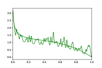
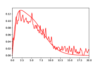
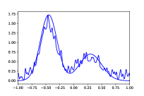
Figure 1: The Beta, Gamma and Gaussian mixtures, respectively. The smooth and coarse plots in each sub-figure correspond to the noise-free and noisy cases, respectively.

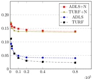
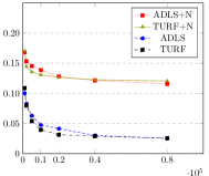
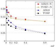
Figure 2: $\ell_{1}$ error versus number of samples on the Beta, Gamma, and Gaussian mixtures respectively in Figure 1 for $d=1$.

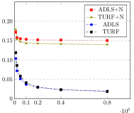
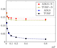
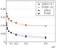
Figure 3: $\ell_{1}$ error versus number of samples on the Beta, Gamma, and Gaussian mixtures respectively in Figure 1 for $d=2$.

Direct comparison of $\mathrm{TURF}$ and $\mathrm{ADLS}$ for a given $t,d$ is not straightforward as $\mathrm{TURF}$ outputs polynomials consisting of more pieces. To compare the algorithms more equitably, we apply the cross-validation technique in Section 6 to select the best $t$ for each. The cross validation parameter $\delta$ is chosen to reflect the actual number of pieces output by $\mathrm{ADLS}$ and $\mathrm{TURF}$. Note that while $\mathrm{SURF}$ (Hao et al., 2020) is another piecewise polynomial based estimation method, it has an implicit method to cross-validate $t$, unlike $\mathrm{ADLS}$ and $\mathrm{TURF}$. As comparisons against $\mathrm{SURF}$ may only reflect the relative strengths of the cross validation methods and not that of the underlying estimation procedure, we defer them to Appendix 5. All experiments compare the $\ell_{1}$ error, run for $n$ between 1,000 and 80,000, and averaged over 50 runs. For $\mathrm{ADLS}$ we use the code provided in (Acharya et al., 2017), and for $\mathrm{TURF}$ we use the algorithm in Section 5.

The experiments consider the structured distributions addressed in (Acharya et al., 2017), namely mixtures of Beta: $.4\text{B}(.8,4)+.6\text{B}(2,2)$, Gamma: $.7\Gamma(2,2)+.3\Gamma(7.5,1)$, and Gaussians: .65${\cal N}$(-.45,$.15^{2}$)+.35${\cal N}$(.3,$.2^{2}$) as shown in Figure 1. Figure 2 considers approximation relative to ${\cal P}_{t,1}$. The blue-dashed and the black-dot-dash plots show that $\mathrm{TURF}$ modestly outperforms $\mathrm{ADLS}$. It is especially significant for the Beta distribution as $\text{B}(.8,4)$ has a large second derivative near $0$, and approximating it may require many degree-1 pieces localized to that region. For this lower width region, the ${\cal A}_{1}$ distance may be too small to warrant many pieces in $\mathrm{ADLS}$, unlike in $\mathrm{TURF}$ that forms intervals guided by shape constraints e.g., based on Lemma 7.

We perturb these distribution mixtures to increase their bias. For a given $k>0$, select $\bar{\mu}_{k}\stackrel{{\scriptstyle\mathrm{def}}}{{=}}(\mu_{1}{,}\ldots{,}\mu_{k})$ by independently choosing $\mu_{i},\ i\in\{1{,}\ldots{,}k\}$ uniformly from the effective support of $f$ (we remove $5\%$ tail mass on either side). At each of these locations, apply a Gaussian noise of magnitude $0.25/k$ with standard deviation $\sigma=c_{2}/k$, for some constant $c_{2}>0$ that is chosen to scale with the effective support width of $f$. That is,

$$f_{\bar{\mu}}\stackrel{{\scriptstyle\mathrm{def}}}{{=}}\frac{3}{4}\cdot f+\frac{1}{4}\cdot\sum_{i=1}^{k}\frac{1}{k}\cdot{\cal N}{\left({\mu_{i},\frac{c_{2}^{2}}{k^{2}}}\right)}.\vspace{-.25em}$$

We choose $k=100$ and $c_{2}=0.05,1,0.1$ for the Beta, Gamma and Gaussian mixtures respectively, to yield the distributions shown in Figure 1. The red-dotted and olive-solid plots in Figure 2 compares $\mathrm{ADLS}$ and $\mathrm{TURF}$ on these distributions. While the overall errors are larger due to the added noise, $\mathrm{TURF}$ outperforms $\mathrm{ADLS}$ on nearly all distributions. A consistent trend across our experiments is that for large $n$, the performance gap between $\mathrm{ADLS}$ and $\mathrm{TURF}$ decreases. This may be explained by the fact that as $n$ increases, the value of $t$ output by the cross-validation method also increases, reducing the bias under both $\mathrm{ADLS}$ and $\mathrm{TURF}$. However, the reduction in $\mathrm{ADLS}$’s bias is more significant due to its larger approximation factor compared to $\mathrm{TURF}$, resulting in the smaller gap.

Figure 3 repeats the same experiments for $d=2$. Increasing the degree leads to lower errors on both $\mathrm{ADLS}$ and $\mathrm{TURF}$ in the non-noisy case. However, the larger bias in the noisy case reveals the improved performance of $\mathrm{TURF}$.

Appendix A Proofs for Section 1

A.1 Proof of Lemma 3

Proof

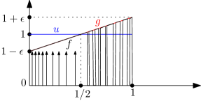
Figure 4: $f$ that is indistinguishable from $u$ in the proof of Lemma 3

Note that for any $t_{1}\leq t$ and $d_{1}\leq d$, ${\cal P}_{t_{1},d_{1}}\subseteq{\cal P}_{t,d}$. Therefore $c_{t,d}$ increases with $t,d$. (Chan et al., 2014) showed that $c_{2,0}\geq 2$. We show below that that $c_{1,1}\geq 2$. Together they imply $c_{t,d}\geq 2$ when $t\geq 2$ or $d\geq 1$.

Let $u$ be the uniform distribution on $[0,1]$. Fix an $\epsilon>0$ and consider the distribution $g(x)=1-\epsilon+2\epsilon x$. Note that $g\in{\cal P}_{1,1}$. For a fixed $k\geq 1$, we construct two random distributions $f_{k}$ and $f_{k}^{\prime}$ that are essentially indistinguishable using $n$ samples as $k$ is made large, and such that all functions have an $\ell_{1}$ distance to either $f_{k}$ or $f_{k}^{\prime}$ that is at least twice as far as their respective $\ell_{1}$ approximations in ${\cal P}_{1,1}$.

To construct $f_{k}$ we perturb $g$ separately on the left, $[0,1/2]$, and right, $(1/2,1]$, halves of $[0,1]$.

For the left half, we use the discrete sub-distribution $h_{k}$ that assigns a mass $\epsilon/4\cdot 1/k$ to $k$ values drawn according to the distribution $h(x)=4-8x$ over $[0,1/2]$. Then let

$$f_{k}(x)=g(x)+h_{k}(x),\text{\quad for\quad}x\in[0,1/2].$$

Thus $f_{k}$ consists of discrete atoms added to $g$ on $[0,1/2]$.

For the right half, assuming Wolog that $k$ is even, first partition $(1/2,1]$ into $k/2$ intervals of width $1/k$ by letting $I_{i}\stackrel{{\scriptstyle\mathrm{def}}}{{=}}(1/2+(i-1)/k,1/2+i/k]$ for $i\in\{1{,}\ldots{,}k/2\}$. Let $|I|$ denote the width of interval $I$. For each $i\in\{1{,}\ldots{,}k/2\}$, select a random circular sub-interval $J_{i}\subseteq I_{i}$ of width

$$w_{i}=\frac{1}{1+2\epsilon i/k}\cdot|I_{i}|$$

as follows: Suppose $I_{i}=[a_{i},b_{i}]$ for simplicity. Choose a point $x_{i}$ uniformly at random in $I_{i}$ and define

$$J_{i}\stackrel{{\scriptstyle\mathrm{def}}}{{=}}[a_{i},a_{i}+\max\{0,x_{i}+w_{i}-b_{i}\}]\cup(x_{i},\min\{x_{i}+w_{i},b_{i}\}].$$

Let $f_{k}$ be $g$ over $J_{i}$ and $0$ over $I_{i}\setminus J_{i}$, hence as illustrated in Figure 4, for $x\in(1/2,1]$,

$$f_{k}(x)\stackrel{{\scriptstyle\mathrm{def}}}{{=}}\begin{cases}g(x)&x\in J_{i},\quad i\in\{1{,}\ldots{,}k/2\},\\ 0&x\in I_{i}\setminus J_{i},\quad i\in\{1{,}\ldots{,}k/2\}.\end{cases}$$

It is easy to show that on any sub-interval of $I_{i}$, the area of $f_{k}$ is within that of $u$ up to an additive ${\cal O}(\epsilon/k)$.

Construct $f_{k}^{\prime}$ via the same method for $f_{k}$ but mirrored along $1/2$, with $g^{\prime}=1+\epsilon-2\epsilon x$, adding atoms to $(1/2,1]$ and alternating between $g^{\prime}$ and $0$ on $[0,1/2]$ as described in the construction of $f_{k}$.

By a birthday paradox type argument, for any $\delta\geq 0$, it is easy to see that the distributions $f_{k}$, $f_{k}^{\prime}$ are indistinguishable from $u$ with probability $\geq 1-\delta$ using any finitely many $n$ samples (by choosing an appropriately large $k=k(\delta,n)$). Thus w.p. $\geq 1-2\delta$, the estimate $f^{\textit{est}}=f^{\textit{est}}_{X^{n}}$ is identical under both $f_{k}$ and $f_{k}^{\prime}$. Therefore any estimator $f^{\textit{est}}$ suffers a factor

$$c\geq(1-2\delta)\cdot\min_{f^{\textit{est}}}\max\Bigg{\{}\frac{\|f^{\textit{est}}-f_{k}\|_{1}}{\|f_{k}-{\cal P}_{1,1}\|_{1}},\frac{\|f^{\textit{est}}-f_{k}^{\prime}\|_{1}}{\|f_{k}^{\prime}-{\cal P}_{1,1}\|_{1}}\Bigg{\}},$$

By the mirror image symmetry between $f_{k}$ and $f_{k}^{\prime}$ about 1/2, $f^{\textit{est}}=u$ is the optimal estimate to within an additive ${\cal O}(\epsilon/k)$. This lower bounds $c$ as

$$\frac{c}{1-2\delta}\geq\frac{\|f_{k}-u\|_{1}-{\cal O}(\epsilon/k)}{\|f_{k}-{\cal P}_{1,1}\|_{1}} \overset{(a)}{\geq}\frac{\|f_{k}-u\|_{1}-{\cal O}(\epsilon/k)}{\|f_{k}-g\|_{1}}$$

$$=\frac{\|f_{k}-u\|_{1,[0,1/2]}+\|f_{k}-u\|_{1,(1/2,1]}-{\cal O}(\epsilon/k)}{\|f_{k}-g\|_{1,[0,1/2]}+\|f_{k}-g\|_{1,(1/2,1]}}$$

$$\overset{(b)}{=}\frac{\|h_{k}\|_{1,[0,1/2]}+\|g-u\|_{1,[0,1/2]}+\|f_{k}-u\|_{1,(1/2,1]}-{\cal O}(\epsilon/k)}{\|h_{k}\|_{1,[0,1/2]}+\|f_{k}-g\|_{1,(1/2,1]}}$$

$$\overset{(c)}{=}\frac{\epsilon/4+\epsilon/4+\|f_{k}-u\|_{1,[1/2,1]}-{\cal O}(\epsilon/k)}{\epsilon/4+\|f_{k}-g\|_{1,(1/2,1]}}$$

$$\overset{(d)}{=}\frac{\epsilon/4+\epsilon/4+\|f_{k}-u\|_{1,[1/2,1]}-{\cal O}(\epsilon/k)}{\epsilon/4+\int_{1/2}^{1}g(x)dx-\int_{1/2}^{1}f_{k}(x)dx}$$

$$=\frac{\epsilon/4+\epsilon/4+\|f_{k}-u\|_{1,[1/2,1]}-{\cal O}(\epsilon/k)}{\epsilon/4+1/2+\epsilon/4-\int_{1/2}^{1}f_{k}(x)dx}$$

$$\overset{(e)}{=}\frac{\epsilon/4+\epsilon/4+\|f_{k}-u\|_{1,[1/2,1]}-{\cal O}(\epsilon/k)}{\epsilon/2+{\cal O}(\epsilon/k)}$$

$$\overset{(f)}{\geq}\frac{\epsilon/4+\epsilon/4+\epsilon/2-{\cal O}(\epsilon/k)}{\epsilon/2+{\cal O}(\epsilon/k)}=2-{\cal O}{\left({\frac{1}{k}}\right)},$$

where $(a)$ follows since $g\in{\cal P}_{1,1}$, $(b)$ follows since $h_{k}$ is a discrete distribution, $(c)$ follows since $h_{k}$ has a total mass $\epsilon/4$ and since $\|g-u\|_{1,[0,1/2]}=\epsilon/4$ by a straightforward calculation, $(d)$ follows since $g\geq f_{k}$ in $(1/2,1]$, $(e)$ follows since the area of $f_{k}$ and $u$ on $I=(1/2,1]$ are equal to within an additive ${\cal O}(\epsilon/k)$, and $(f)$ follows since $\|f_{k}-u\|_{1,(1/2,1]}\geq 2\|f_{k}-g\|_{1,(1/2,1]}-{\cal O}(\epsilon/k)$. Choosing $\delta\searrow 0$ and $k\nearrow\infty$ completes the proof.

A.2 Description and proof of Lemma 17

The following lemma shows that if $f^{\textit{est}}$ is a $c$-factor approximation for ${\cal P}_{t,d}$ for some $t$ and $d$ and achieves the min-max rate of a distribution class ${\cal C}$, then $f^{\textit{est}}$ is also a $c$-factor approximation for ${\cal C}$.

Lemma 17.

If $f^{\textit{est}}$ is a $c$-factor approximation for ${\cal P}_{t,d}$ and for all $f$ in a class ${\cal C}$, $c\cdot\|f-{\cal P}_{t,d}\|_{1}+{\cal O}({\cal R}_{n}({{\cal P}_{t,d})})\leq{\cal O}({\cal R}_{n}({\cal C}))$, then for any $f$, not necessarily in ${\cal C}$,

$$\|f^{\textit{est}}-f\|_{1}\leq c\cdot\|f-{\cal C}\|_{1}+{\cal O}({\cal R}_{n}({\cal C})).$$

Proof  For a distribution $g$ and class ${\cal D}$, let $g_{{\cal D}}\in{\cal D}$ be the closest approximation to $g$ from ${\cal D}$, namely achieving $\|g-g_{{\cal D}}\|_{1}=\|g-{\cal D}\|_{1}$. Then for any distribution $f$,

$$\|f^{\textit{est}}-f\|_{1} \leq c\cdot\|f-{\cal P}_{t,d}\|_{1}+{\cal O}{\left({{\cal R}_{n}({\cal P}_{t,d})}\right)}$$

$$\overset{(a)}{\leq}c\cdot\|f-f_{{\cal C}_{{\cal P}_{t,d}}}\|_{1}+{\cal O}{\left({{\cal R}_{n}({\cal P}_{t,d})}\right)}$$

$$\leq c\cdot\|f-f_{{\cal C}}\|_{1}+c\cdot\|f_{{\cal C}_{{\cal P}_{t,d}}}-f_{{\cal C}}\|_{1}+{\cal O}{\left({{\cal R}_{n}({\cal P}_{t,d})}\right)}$$

$$\overset{(b)}{=}c\cdot\|f-{\cal C}\|_{1}+c\cdot\|f_{{\cal C}}-{\cal P}_{t,d}\|_{1}+{\cal O}{\left({{\cal R}_{n}({\cal P}_{t,d})}\right)}$$

$$\overset{(c)}{=}c\cdot\|f-{\cal C}\|_{1}+{\cal O}{\left({{\cal R}_{n}({{\cal C}})}\right)},$$

where in $(a)$, just as $f_{{\cal C}}$ is the ${\cal C}$ distribution closest to $f$, $f_{{\cal C}_{{\cal P}_{t,d}}}$ is the ${\cal P}_{t,d}$ distribution closest to $f_{{\cal C}}$ and the inequality follows since $f_{{\cal C}_{{\cal P}_{t,d}}}\in{\cal P}_{t,d}$ and by definition, $\|f-{\cal P}_{t,d}\|_{1}$ is the least distance from $f$ to any $q\in{\cal P}_{t,d}$, $(b)$ follows since by definition, $f_{{\cal C}_{{\cal P}_{t,d}}}$ is the best approximation to $f_{{\cal C}}$ from ${\cal P}_{t,d}$, and $(c)$ follows from the property of ${\cal C}$ considered in the lemma as $f_{{\cal C}}\in{\cal C}$.

Appendix B Proofs for Section 4

B.1 Proof of Lemma 7

Proof  Observe that for any $q\in{\cal P}_{d}$ and interval $J$,

$$\Delta_{J}(q)\stackrel{{\scriptstyle\mathrm{def}}}{{=}}\max_{x\in J}q(x)-\min_{x\in J}q(x)\leq\int_{J}|q^{\prime}(t)|dt,$$

where $q^{\prime}$ denotes the first derivative of $q$. The case of $d=0$ is trivial. We give a proof for $d\geq 1$. Consider

$$f_{d}(x)\,\stackrel{{\scriptstyle\mathrm{def}}}{{=}}\,\frac{1}{\text{\normalsize$x$}}\sin(d\arcsin(x)).$$

The following two claims (indicated with the overset (*)) may be verified via Wolfram Mathematica e.g. version 12.3.
Claim 1 $\lvert\lvert f_{d}\rvert\rvert_{2}\leq\sqrt{\pi\,d}$,  because

$$\lvert\lvert f_{d}\rvert\rvert_{2}^{2} \overset{(*)}{=}2\int_{0}^{1}\frac{\sin^{2}(d\arcsin(x))}{x^{2}}\,\,dx\leq\int_{0}^{\frac{\pi}{2}}\frac{1-\cos(2d\theta)}{\sin^{2}\theta}\,d\theta\overset{}{=}\pi\,d.$$

Claim 2 $f_{d}(0)\overset{(*)}{=}d$ and $f^{\prime}_{d}(0)\overset{(*)}{=}0$.
Let $f(t)\stackrel{{\scriptstyle\mathrm{def}}}{{=}}q(t)\sqrt{1-t^{2}}$ and note that for any $x\in[0,1]$,

$$\sqrt{1-x^{2}}\int_{-x}^{x}|q^{\prime}(t)|\,dt \leq\int_{-1}^{1}|q^{\prime}(t)|\sqrt{1-t^{2}}\,dt\leq\int_{-1}^{1}|f^{\prime}(t)|\,dt+\int_{-1}^{1}\frac{|t\,q(t)|}{\sqrt{1-t^{2}}},dt,$$

where the final inequality follows by integration by parts.

For simplicity let $g_{d}(x)\stackrel{{\scriptstyle\mathrm{def}}}{{=}}\sqrt{\frac{2}{\pi d}}\cdot f_{\frac{d}{2}}(x)$, then $g_{d}(0)=\sqrt{\frac{d}{2\pi}}$ and $g^{\prime}_{d}(0)=0$. Hence,

$$\frac{1}{2\pi}|f^{\prime}(0)| =\frac{1}{d}\,|f^{\prime}(0)|\,g^{2}_{d}(0){\overset{(a)}{\leq}}2\max_{t}|f(t)|\,g^{2}_{d}(t){\overset{(b)}{\leq}}4d\int_{-1}^{1}|q(t)|\,g^{2}_{d}(t)\,dt,$$

where $(b)$ follows from Bernstein’s inequality since $|q(t)|\sqrt{1-t^{2}}\leq d\int_{-1}^{1}|q(z)|dz$ for a degree-$d$ polynomial $q$ and any $t\in[0,1]$, and applying the inequality to $q(t)g_{d}^{2}(t)$ of degree $2d-2$. For $(a)$ we apply Bernstein’s inequality to $q(z)=\frac{d}{dz}{\left({f(z)g^{2}_{d}(z)}\right)}$, set $t=0$ and notice that $g_{d}^{\prime}(0)=0$.
Equivalently by a change of variables, for $c\,\stackrel{{\scriptstyle\mathrm{def}}}{{=}}8\pi$ and $f_{\text{\tiny T}}(\theta)\stackrel{{\scriptstyle\mathrm{def}}}{{=}}f(\sin\theta)$,

$$|f_{\text{\tiny T}}^{\prime}(0)|=|f^{\prime}(0)|\leq c\ d\int_{-1}^{1}|q(t)|\,g^{2}_{d}(t)\,dt\leq c\,d\int_{-\pi}^{\pi}|f_{\text{\tiny T}}(\theta)|\,g^{2}_{d}(\sin\theta)d\theta.$$

Using the same reasoning for $f_{\text{\tiny T}}(\theta+\alpha)$ instead of $f_{\text{\tiny T}}(\theta)$ we obtain

$$|f_{\text{\tiny T}}^{\prime}(\alpha)|\leq c\,d\int_{-\pi}^{\pi}|f_{\text{\tiny T}}(\theta+\alpha)|\,g^{2}_{d}(\sin\theta)\,d\theta=c\,d\int_{-\pi}^{\pi}|f_{\text{\tiny T}}(\theta)|\,g^{2}_{d}(\sin(\theta-\alpha))\,d\theta,$$

where the equality follows since $|f_{\text{\tiny T}}(\theta+\alpha)|\,g^{2}_{d}(\sin(\theta))$ is a periodic function with period $2\pi$. Integrating both sides for $\alpha$ from $-\pi$ to $\pi$ yields

$$\int_{-1}^{1}|f^{\prime}(t)|\,dt=\int_{-\pi}^{\pi}|f_{\text{\tiny T}}^{\prime}(\alpha)|\,d\alpha\,{\overset{(a)}{\leq}}\,c\,d\int_{-\pi}^{\pi}|f_{\text{\tiny T}}(\theta)|\,d\theta=c\,d\int_{-1}^{1}|q(t)|\,dt,$$

where (a) follows since $\lvert\lvert g_{d}\rvert\rvert_{2}\leq 1$ from Claim 1 and the definition of $g_{d}$. Finally, for a proper $\tau\in(0,1)$ of order $1/d^{2}$,

$$\int_{-1}^{1}\frac{|t\,q(t)|}{\sqrt{1-t^{2}}}\,dt \leq\int_{-1+\tau}^{1-\tau}\frac{|q(t)|}{\sqrt{1-t^{2}}}\,dt+2\max_{t}|q(t)|\int_{1-\tau}^{1}\frac{t}{\sqrt{1-t^{2}}}\,dt$$

$${\overset{(a)}{\leq}}\frac{\int_{-1}^{1}|q(t)|\,dt}{\sqrt{2\tau-\tau^{2}}}+2\max_{t}|q(t)|\int_{1-\tau}^{1}\frac{t}{\sqrt{1-t^{2}}}\,dt$$

$${=}\frac{\int_{-1}^{1}|q(t)|\,dt}{\sqrt{2\tau-\tau^{2}}}+2\max_{t}|q(t)|\cdot\sqrt{2\tau-\tau^{2}}$$

$${\overset{(b)}{\leq}}\frac{\int_{-1}^{1}|q(t)|\,dt}{\sqrt{2\tau-\tau^{2}}}+2\sqrt{2\tau-\tau^{2}}\cdot(d+1)^{2}\int_{-1}^{1}|q(t)|\,dt$$

$$\overset{(c)}{=}{2\sqrt{2}}(d+1)\int_{-1}^{1}|q(t)|\,dt,$$

where $(a)$ follows since $1/\sqrt{1-t^{2}}\leq 1/\sqrt{2\tau-\tau^{2}}$ for $t\in[-1+\tau,1-\tau]$, $(b)$ follows from the Markov Brothers’ inequality, and $(c)$ holds for some $\tau={\cal O}(1/d^{2})$. Proof is complete from the fact that $8\pi+2\sqrt{2}<28$.

B.2 Proof of Lemma 8

Since for any $i\in\{1{,}\ldots{,}m\}$, $\bar{I}_{i}^{+}\in\bar{I}^{+}$ and $\bar{I}_{i}^{-}\in\bar{I}^{-}$ both have $\lceil\ell(d+1)/2^{i/4}\rceil$ intervals for $i\in\{1{,}\ldots{,}m\}$, it follows that the total number of intervals in $(\bar{I}^{-},\bar{I}^{+})$ is upper bounded as

$$2{\left({\sum_{i=1}^{m}|\bar{I}_{i}|+1}\right)} =2{\left({\sum_{i=1}^{m}\Bigg{\lceil}\frac{\ell(d+1)}{2^{i/4}}\Bigg{\rceil}+1}\right)}$$

$$\leq 2{\left({\sum_{i=1}^{m}{\left({\frac{\ell(d+1)}{2^{i/4}}+1}\right)}+1}\right)}$$

$$\leq 2{\left({\sum_{i=1}^{\infty}\frac{\ell(d+1)}{2^{i/4}}+m+1}\right)}$$

$$=2{\left({\frac{\ell(d+1)}{2^{1/4}}\cdot\frac{1}{1-2^{-1/4}}+\log_{2}(\ell(d+1)^{2})+1}\right)}$$

$$\overset{(a)}{\leq}2{\left({\frac{\ell(d+1)}{2^{1/4}}\cdot\frac{1}{1-2^{-1/4}}+2\log_{2}(\ell(d+1))+1}\right)}$$

$$\overset{(b)}{\leq}2{\left({\frac{\ell(d+1)}{2^{1/4}}\cdot\frac{1}{1-2^{-1/4}}+\frac{2\ell(d+1)}{\log 2}}\right)}$$

$$\overset{}{=}2\ell(d+1){\left({\frac{1}{2^{1/4}-1}+\frac{2}{\log 2}}\right)}$$

$$\leq\frac{4\ell(d+1)}{2^{1/4}-1}.$$

where $(a)$ follows since $\ell\geq 1$ and $(b)$ follows from the identity that for any $x\geq 1,\log(x)\leq x-1$.

B.3 Proof of Lemma 9

Proof  We provide a proof for $I=[-1,1]$ by considering $\bar{I}=\overline{[-1,1]}^{d,k}$. An identical proof follows for any other interval $I$ as its partition $\overline{I}^{d,k}$ is obtained by a linear translation of $\overline{[-1,1]}^{d,k}$. For $i\in\{1{,}\ldots{,}m\}$, let

$$I_{i}\stackrel{{\scriptstyle\mathrm{def}}}{{=}}I_{i}^{+}\cup I_{i}^{-}.$$

Similarly let ${E}_{m}\stackrel{{\scriptstyle\mathrm{def}}}{{=}}{E}_{m}^{+}\cup{E}_{m}^{-}$. Applying Lemma 7 with $a={1-1/2^{i}}$, we obtain

$$\int_{I_{i}}|p^{\prime}(x)|dx\overset{(a)}{\leq}\int_{-{\left({1-1/2^{i}}\right)}}^{{\left({1-1/2^{i}}\right)}}|p^{\prime}(x)|dx \overset{}{\leq}\frac{28(d+1){\|p\|}_{1,I}}{(1-{\left({1-1/2^{i}}\right)}^{2})^{1/2}}$$

$$\leq\frac{28(d+1){\|p\|}_{1,I}}{(1-{\left({1-1/2^{i}}\right)})^{1/2}}$$

$$\leq 28\cdot 2^{i/2}\cdot(d+1){\|p\|}_{1,I},$$

where $(a)$ follows since $I_{i}\subseteq[-{\left({1-1/2^{i}}\right)},{\left({1-1/2^{i}}\right)}]$. As $\bar{I}_{i}^{+}$ consists of $\lceil\ell(d+1)/2^{i/4}\rceil$ equal width intervals from Equation (4) and since $\bar{I}_{i}^{+}$ is of width $|\bar{I}_{i}^{+}|=1/2^{i}$, it follows that each interval in $\bar{I}_{i}^{+}$ (and similarly for $\bar{I}^{-}$) is of width $\leq 1/(2^{3i/4}\cdot l(d+1))$. Thus from Equation (2), the $\ell_{1}$ difference between $p$ and $\bar{p}_{\bar{I}}$ over $I_{i}$ is given by

$$\|p-\bar{p}_{\bar{I}}\|_{1,I_{i}} \leq\sum_{J\in\bar{I}_{i}}\Delta_{J}(p)\cdot|J|$$

$$\leq\sum_{J\in\bar{I}_{i}}\Delta_{I_{i}}(p)\cdot\frac{1}{2^{3i/4}\cdot\ell(d+1)}$$

$$\leq{\left({\sum_{J\in\bar{I}_{i}}\int_{J}|p^{\prime}(x)|dx}\right)}\cdot\frac{1}{2^{3i/4}\cdot\ell(d+1)}$$

$$\leq\int_{I_{i}}|p^{\prime}(x)|dx\cdot\frac{1}{2^{3i/4}\cdot\ell(d+1)}$$

$$\leq 28\cdot 2^{i/2}\cdot(d+1){\|p\|}_{1,I}.\frac{1}{2^{3i/4}\cdot\ell(d+1)}=\frac{28\cdot 2^{-i/4}{\|p\|}_{1,I}}{\ell}.$$

Therefore

$$\|p-\bar{p}_{\bar{I}}\|_{1,I} =\sum_{i=1}^{m}\|p-\bar{p}_{\bar{I}}\|_{1,I_{i}}+\|p-\bar{p}_{\bar{I}}\|_{1,{E}_{m}}$$

$$\leq\sum_{i=1}^{m}\frac{28\cdot 2^{-i/4}{\|p\|}_{1,I}}{\ell}+\max_{x\in{E}_{m}}{p(x)}\cdot\frac{2}{\ell(d+1)^{2}}$$

$$\overset{(a)}{\leq}\sum_{i=1}^{m}\frac{28\cdot 2^{-i/4}{\|p\|}_{1,I}}{\ell}+(d+1)^{2}{\|p\|}_{1,I}\frac{2}{\ell(d+1)^{2}}$$

$$\overset{(b)}{\leq}\frac{{\|p\|}_{1,I}}{\ell}{\left({\frac{28}{1-2^{-1/4}}+2}\right)}$$

$$\overset{(c)}{\leq}\frac{4(d+1){\|p\|}_{1,I}}{k(2^{1/4}-1)}{\left({\frac{28}{1-2^{-1/4}}+2}\right)}$$

$$\overset{}{\leq}\frac{3764(d+1){\|p\|}_{1,I}}{k},$$

where $(a)$ follows since $I$ is a symmetric interval, $\forall x\in I$, $p(x)\leq(d+1)^{2}{\|p\|}_{1,I}$ from the Markov Brothers’ inequality, $(b)$ follows from the infinite negative geometric sum and $(c)$ follows since $\ell\stackrel{{\scriptstyle\mathrm{def}}}{{=}}k(2^{1/4}-1)/(4(d+1))$ as defined in Equation (4).

B.4 Proof of Lemma 11

Proof  Select a $p^{*}\in{\cal P}_{d}$ that achieves $\|f-p^{*}\|_{1,I}=\|f-{\cal P}_{d}\|_{1,I}$. Then

$$\|f^{\textit{adj}}-f\|_{1,I} \leq\|f^{\textit{adj}}-p^{*}\|_{1,I}+\|p^{*}-f\|_{1,I}$$

$$\overset{(a)}{\leq}2\cdot\|f-p^{*}\|_{1,I}+\frac{c_{1}(d+1)\|p^{*}-f^{\textit{poly}}\|_{1,I}}{k}+\|f^{\textit{emp}}-f\|_{{\cal A}_{k},I}$$

$$\leq 2\cdot\|f-p^{*}\|_{1,I}+\frac{c_{1}(d+1){\left({\|p^{*}-f\|_{1,I}+\|f-f^{\textit{poly}}\|_{1,I}}\right)}}{k}+\|f^{\textit{emp}}-f\|_{{\cal A}_{k},I}$$

$$\overset{(b)}{\leq}{\left({2+\frac{c_{1}(d+1)(1+c^{\prime})}{k}}\right)}\|f-p^{*}\|_{1,I}+{\left({\frac{c_{1}(d+1)c^{\prime\prime}}{k}+1}\right)}\|f^{\textit{emp}}-f\|_{{\cal A}_{k},I}+\frac{c_{1}(d+1)}{k}\cdot{\eta},$$

where $(a)$ follows from setting $p=p^{*}$ in Lemma 10, and $(b)$ follows from using $\|f^{\textit{poly}}-f\|_{1,I}\leq c^{\prime}\|f-p^{*}\|_{1,I}+c^{\prime\prime}\|f^{\textit{emp}}-f\|_{{\cal A}_{d+1},I}+\eta$ along with the fact that $k\geq d+1$ (so that $\|f^{\textit{emp}}-f\|_{{\cal A}_{d+1},I}\leq\|f^{\textit{emp}}-f\|_{{\cal A}_{k},I}$).

B.5 Proof of Theorem 12

Proof  Since $c=3$ and $c^{\prime}=2$ for the $f^{\textit{adls}}$ estimate, it follows for $I=[X_{(0)},X_{(n)}]$ from Lemma 11 that

$$\|f^{\textit{adj}}-f\|_{1,I} \leq{\left({2+\frac{3c_{1}(d+1)}{k}}\right)}\|f-p^{*}\|_{1}+{\left({\frac{2c_{1}(d+1)}{k}+1}\right)}\|f^{\textit{emp}}-f\|_{{\cal A}_{d+1}}+\frac{c_{1}(d+1)}{k}\cdot{\eta_{d}}$$

$$\leq{\left({2+\gamma}\right)}\|f-{\cal P}_{d}\|_{1}+{\left({\frac{\gamma}{4}+1}\right)}\|f^{\textit{emp}}-f\|_{{\cal A}_{d+1}}+\frac{\gamma}{8}\cdot{\eta_{d}}$$

where the last inequality follows since we choose $k=k(\gamma)\geq 8c_{1}(d+1)/\gamma$. Let $J=\mathbb{R}\setminus I$. Using Lemma 4,

$$\operatorname*{\mathbb{E}}\|f^{\textit{adj}}-f\|_{1} \leq{\left({2+\gamma}\right)}\|f-{\cal P}_{d}\|_{1,I}+{\left({\frac{\gamma}{4}+1}\right)}\operatorname*{\mathbb{E}}\|f^{\textit{emp}}-f\|_{{\cal A}_{d+1}}+\frac{\gamma}{8}\cdot{\eta_{d}}+{\left({2+\gamma}\right)}{\|f\|}_{1,J}$$

$$={\left({2+\gamma}\right)}\|f-{\cal P}_{d}\|_{1,I}+{\left({\frac{\gamma}{4}+1}\right)}\operatorname*{\mathbb{E}}\|f^{\textit{emp}}-f\|_{{\cal A}_{d+1}}+\frac{\gamma}{8}\cdot{\eta_{d}}+{\left({2+\gamma}\right)}\operatorname*{\mathbb{E}}\|f-f^{\textit{emp}}\|_{{\cal A}_{2},J}$$

$$\overset{(a)}{\leq}{\left({2+\gamma}\right)}\|f-{\cal P}_{d}\|_{1,I}+{\left({\frac{\gamma}{4}+1}\right)}{\cal O}{\left({\sqrt{\frac{k}{n}}}\right)}+\frac{\gamma}{8}\cdot{\eta_{d}}+3\cdot{\cal O}{\left({\sqrt{\frac{2}{n}}}\right)}$$

$$\overset{(b)}{\leq}{\left({2+\gamma}\right)}\|f-{\cal P}_{d}\|_{1}+{\cal O}{\left({\sqrt{\frac{d+1}{\gamma\cdot n}}}\right)},$$

where $(a)$ follows since $\gamma<1$ and from Lemma 4, and $(b)$ follows as $\eta_{d}=\sqrt{(d+1)/n}$, $k={\cal O}(d+1)$ and $0<\gamma<1$.

Appendix C Proofs for Section 5

C.1 Proof of Theorem 13

From Lemma 14,

$$\|f^{\textit{out}}_{t,d,\alpha}-f\|_{1} \leq{\left({2+\frac{4c_{1}(d+1)}{k}+\frac{1+k/(d+1)}{\beta-1}}\right)}\|f-{\cal P}_{t,d}\|_{1}+{\left({3+2c_{1}+\frac{2}{\beta-1}}\right)}\|f^{\textit{emp}}-f\|_{{\cal A}_{2\beta t\cdot k}}$$

$$\phantom{\leq}+{\left({\frac{c_{1}(d+1)}{k}+\frac{k}{(\beta-1)(d+1)}}\right)}\eta_{d}$$

$$\overset{(a)}{\leq}{\left({2+\frac{4c_{1}(d+1)}{k}+\frac{\alpha(d+1)}{4k}\cdot{\left({1+\frac{k}{d+1}}\right)}}\right)}\|f-{\cal P}_{t,d}\|_{1}+{\left({3+2c_{1}+\frac{\alpha(d+1)}{2k}}\right)}\|f^{\textit{emp}}-f\|_{{\cal A}_{2\beta t\cdot k}}$$

$$\phantom{\leq}+{\left({\frac{c_{1}(d+1)}{k}+\frac{\alpha(d+1)}{4k}\cdot\frac{k}{d+1}}\right)}\eta_{d}$$

$$\overset{(b)}{\leq}{\left({2+\frac{\alpha}{2}+\frac{\alpha}{2}}\right)}\|f-{\cal P}_{t,d}\|_{1}+{\left({3+2c_{1}+\frac{\alpha}{2}}\right)}\|f^{\textit{emp}}-f\|_{{\cal A}_{2\beta t\cdot k}}+{\left({\frac{\alpha}{8}+\frac{\alpha}{4}}\right)}\eta_{d}$$

where $(a)$ follows since by definition $\beta-1={4k}/(\alpha(d+1))$, $(b)$ follows since $k\stackrel{{\scriptstyle\mathrm{def}}}{{=}}\lceil{8c_{1}(d+1)}/{\alpha}\rceil$ and since $0<\alpha<1$, $c_{1}>1$ imply $k\geq d+1$. From Lemma 4,

$$\operatorname*{\mathbb{E}}\|f^{\textit{out}}_{t,d,\alpha}-f\|_{1} \leq{\left({2+\alpha}\right)}\|f-{\cal P}_{t,d}\|_{1}+{\left({3+2c_{1}+\frac{\alpha}{2}}\right)}\operatorname*{\mathbb{E}}\|f^{\textit{emp}}-f\|_{{\cal A}_{2\beta t\cdot k}}+\frac{3\alpha\eta_{d}}{8}$$

$$\overset{}{\leq}{\left({2+\alpha}\right)}\|f-{\cal P}_{t,d}\|_{1}+{\left({3+2c_{1}+\frac{\alpha}{2}}\right)}{\cal O}{\left({\sqrt{\frac{2\beta tk}{n}}}\right)}+\frac{3\alpha\eta_{d}}{8}$$

$$\overset{(a)}{\leq}{\left({2+\alpha}\right)}\|f-{\cal P}_{t,d}\|_{1}+{\left({3+2c_{1}+\frac{\alpha}{2}}\right)}{\cal O}{\left({\sqrt{\frac{k^{2}t}{\alpha(d+1)}}}\right)}+\frac{3\alpha\eta_{d}}{8}$$

$$\overset{(b)}{\leq}{\left({2+\alpha}\right)}\|f-{\cal P}_{t,d}\|_{1}+{\left({3+2c_{1}+\frac{\alpha}{2}}\right)}{\cal O}{\left({\sqrt{\frac{c_{1}^{2}(d+1)^{2}t}{\alpha^{3}(d+1)n}}}\right)}+\frac{3\alpha\eta_{d}}{8}$$

$$\overset{(c)}{\leq}{\left({2+\alpha}\right)}\|f-{\cal P}_{t,d}\|_{1}+{\cal O}{\left({\sqrt{\frac{t(d+1)}{\alpha^{3}n}}}\right)},$$

where $(a)$, $(b)$ both follow from the definitions of $\beta$, $k$ in Equations (7), (6) and $(c)$ follows since $n_{d}\stackrel{{\scriptstyle\mathrm{def}}}{{=}}\sqrt{(d+1)/n}$ and $0<\alpha<1$.

C.2 Proof of Lemma 14

For simplicity denote $f^{\textit{out}}\stackrel{{\scriptstyle\mathrm{def}}}{{=}}f^{\textit{out}}_{t,d,\alpha}$ and consider a particular $p^{*}\in{\cal P}_{t,d}$ that achieves $\|f-{\cal P}_{t,d}\|_{1}$. Let $\bar{F}$ denote the set of intervals in $\bar{I}_{\mathrm{ADLS}}$ that has $p^{*}$ as a single piece polynomial in $I$. Let $\bar{J}\stackrel{{\scriptstyle\mathrm{def}}}{{=}}\bar{I}_{\mathrm{ADLS}}\setminus\bar{F}$ be the remaining intervals where $p^{*}$ has more than one polynomial piece. Since $p^{*}\in{\cal P}_{t,d}$ has $t$ polynomial pieces, the number of intervals in $\bar{J}$ is $\leq t$.

Recall that for any subset $S\subseteq\mathbb{R}$, and integrable functions $g_{1}$, $g_{2}$, and integer $m\geq 1$, $\|g_{1}-g_{2}\|_{1,S}$, $\|g_{1}-g_{2}\|_{{\cal A}_{m},S}$ denote the $\ell_{1}$ and ${\cal A}_{m}$ distances over $S$ respectively. Equation (14) in (Acharya et al., 2017) shows that over $\bar{F}$,

$$\sum_{I\in\bar{F}}\|f^{\textit{adls}}_{I}-f\|_{1}\leq \ 3\|f-p^{*}\|_{1,\bar{F}}+2||f^{\textit{emp}}-f||_{{\cal A}_{|\bar{F}|\cdot(d+1)},\bar{F}}+\eta_{d}.$$ (9)

We bound the error in $\bar{F}$ by setting $p=p^{*},\ f^{\textit{poly}}=f^{\textit{adls}}_{I}$ in Lemma 10, using Equation (9), and noting that $k\geq d+1$ as $c_{1}\geq 1$ from Equation (6):

$$\sum_{I\in\bar{F}}\|f^{\textit{out}}-f\|_{1,I} \leq 2\sum_{I\in\bar{F}}\|f-p^{*}\|_{1,I}+||f^{\textit{emp}}-f||_{{\cal A}_{k\cdot|\bar{F}|}}+\frac{c_{1}(d+1)}{k}(\|p^{*}-f\|_{1}+\|f-f^{\textit{adls}}_{I}\|_{1})$$

$$\leq\ 2\|f-p^{*}\|_{1,\bar{F}}+(1+2c_{1})||f^{\textit{emp}}-f||_{{\cal A}_{k\cdot|\bar{F}|}}+\frac{c_{1}(d+1)}{k}{\left({4\|f-p^{*}\|_{1}+\eta_{d}}\right)}.$$ (10)

From Lemma 49 (Acharya et al., 2017), for all intervals $I\in\bar{J}$, the following Equation (11) holds that they use to derive Equation (12).

$$\|f^{\textit{adls}}_{I}-f^{\textit{emp}}\|_{{\cal A}_{d+1},I} \leq\frac{\|f-p^{*}\|_{1}+\|f^{\textit{emp}}-f\|_{{\cal A}_{{2\beta t\cdot(d+1)}}}+\eta_{d}}{(\beta-1)t}.$$ (11)

$$\sum_{I\in\bar{J}}\|f^{\textit{adls}}_{I}-f\|_{1,I} \leq\frac{\|f-p^{*}\|_{1}+\|f^{\textit{emp}}-f\|_{{\cal A}_{2\beta t\cdot(d+1)}}}{\beta-1}+2\|f^{\textit{emp}}-f\|_{{\cal A}_{2\beta t\cdot(d+1)}}+{2}\|f-p^{*}\|_{1,\bar{J}}+\frac{\eta_{d}}{2(\beta-1)}.$$ (12)

Recall that we obtain $f^{\textit{out}}$ by adding a constant to $f^{\textit{adls}}_{I}$ along each interval $I\in\overline{I}^{d,k}$ to match its area to $f^{\textit{emp}}$ in that interval. Since $\overline{I}^{d,k}$ has $\leq k$ intervals (Lemma 8), $\forall I\in\bar{J}$,

$$\|f^{\textit{out}}-f^{\textit{adls}}_{I}\|_{1,I} \leq\|f^{\textit{adls}}_{I}-f^{\textit{emp}}\|_{{\cal A}_{k},I}$$

$$\leq\frac{k}{d+1}\|f^{\textit{adls}}_{I}-f^{\textit{emp}}\|_{{\cal A}_{d+1},I}$$ (13)

where the last inequality follows from Property 6.

Adding Equations (12) and (13) over intervals in $\bar{J}$ by noting $\bar{J}$ has $\leq t$ intervals and $k\geq d+1$ implies

$$\sum_{I\in\bar{J}}\|f^{\textit{out}}-f\|_{1,I}\leq {\frac{1+k/(d+1)}{\beta-1}}\cdot\|f-p^{*}\|_{1}+2\|f-p^{*}\|_{1,\bar{J}}+2{\left({1+\frac{1}{\beta-1}}\right)}\|f^{\textit{emp}}-f\|_{{\cal A}_{2\beta t\cdot k}}$$

$$+\frac{k\cdot\eta_{d}}{(d+1)(\beta-1)}.$$ (14)

Adding Equations (10) and (14) proves Lemma 14 (since $p^{*}$ satisfies $\|f-p^{*}\|_{1}=\|f-{\cal P}_{t,d}\|_{1}$).

Appendix D Proofs for Section 6

D.1 Proof of Theorem 15

Proof  Applying the probabilistic version of the VC inequality, i.e. Lemma 4, (see (Devroye & Lugosi, 2012)) to Lemma 14 we have with probability $\geq 1-\delta$,

$$\|f^{\textit{out}}_{t,d,\alpha}-f\|_{1}\leq c\cdot\|f-{\cal P}_{t,d}\|_{1}+{\cal O}{\left({\sqrt{\frac{t(d+1)+\log 1/\delta}{n}}}\right)}.$$

From the union bound, the above condition holds true for the $\log n$ sized estimate collection $\{f^{\textit{out}}_{t,d,\alpha}:t\in\{1,2,4{,}\ldots{,}n\}\}$ with probability $\geq 1-\delta\cdot\log n$. Apply the method discussed in Section 6.2 with $\gamma=2+2/\beta$, to obtain $t^{\textit{est}}=t^{\textit{est}}_{\beta}$. Using Lemma 16 that w.p. $\geq 1-\delta\cdot\log n$,

$$\|f^{\textit{out}}_{t^{\textit{est}},d,\alpha}-f\|_{1} \overset{}{\leq}\min_{t\in\{1,2,4{,}\ldots{,}n\},d}{\left({{\left({1+\frac{2}{\gamma-2}}\right)}\cdot c\cdot\|f-{\cal P}_{t,d}\|_{1}+(\gamma+1)\chi{\sqrt{\frac{t(d+1)}{n}}}}\right)}$$

$$\overset{(a)}{\leq}\min_{0\leq t\leq n,d}{\left({{\left({1+\frac{2}{\gamma-2}}\right)}\cdot c\cdot\|f-{\cal P}_{t,d}\|_{1}+\sqrt{2}(\gamma+1)\chi{\sqrt{\frac{t(d+1)+\log 1/\delta}{n}}}}\right)}$$

$$\overset{(b)}{\leq}\min_{0\leq t\leq n,d}{\left({{\left({1+\beta}\right)}\cdot c\cdot\|f-{\cal P}_{t,d}\|_{1}+{\cal O}{\left({{\sqrt{\frac{t(d+1)+\log 1/\delta}{\beta^{2}n}}}}\right)}}\right)},$$

where $(a)$ follows from the fact that for any $1\leq t\leq n$, $\exists t^{\prime}\in\{1,2,4{,}\ldots{,}n\}:t^{\prime}\in[t,2t]$ (so that $\|f-{\cal P}_{t^{\prime},d}\|_{1}\leq\|f-{\cal P}_{t,d}\|_{1}$ and $(b)$ follows since $\gamma=2+2/\beta$.

D.2 Proof of Lemma 16

Proof  For $i\geq i_{\gamma}$, from the triangle inequality, and as by definition, $d{\left({{v_{i_{\gamma}}},{v_{i}}}\right)}\leq\gamma c_{i}$ for all $i\geq i_{\gamma}$,

$$d{\left({{v_{i_{\gamma}}},{v}}\right)} \leq d{\left({{v_{i}},{v}}\right)}+d{\left({{v_{i_{\gamma}}},{v_{i}}}\right)}\leq b_{i}+c_{i}+\gamma c_{i}=b_{i}+(1+\gamma)c_{i}.$$

For $i<i_{\gamma}$, if

$$b_{i_{\gamma}-1}\geq\frac{\gamma-2}{2}c_{i_{\gamma}},$$

the proof follows since for any $1\leq j^{\prime}\leq i_{\gamma}-1$,

$$d{\left({{v_{i_{\gamma}}},{v}}\right)}\leq b_{i_{\gamma}}+c_{i_{\gamma}}\leq b_{i_{\gamma}}+\frac{2}{\gamma-2}b_{j}\overset{(a)}{\leq}{\left({1+\frac{2}{\gamma-2}}\right)}b_{j^{\prime}},$$

where $(a)$ follows since $j^{\prime}\leq j<i_{\gamma}$. On the other hand if

$$b_{i_{\gamma}-1}<\frac{\gamma-2}{2}c_{i_{\gamma}},$$

then $\forall j^{\prime\prime}\geq j+1$,

$$d{\left({{v_{j}},{v_{j^{\prime\prime}}}}\right)}\leq b_{j}+b_{j^{\prime\prime}}+c_{j}+c_{j^{\prime\prime}}\overset{(a)}{\leq}2b_{j}+2c_{j^{\prime\prime}}\leq 2\cdot\frac{\gamma-2}{2}c_{i_{\gamma}}+2c_{j^{\prime\prime}}\overset{(b)}{\leq}\gamma c_{j^{\prime\prime}},$$

where $(a)$ follows since $j^{\prime\prime}\geq j$, and $(b)$ follows since $j^{\prime\prime}\geq j=i_{\gamma}$, contradicting the definition of $i_{\gamma}$.

Appendix E Additional Experiments

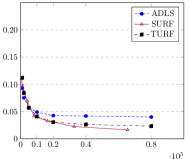
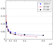
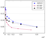
Figure 5: $\ell_{1}$ error versus number of samples on the Beta, Gamma, and Gaussian mixtures respectively in Figure 1 for $d=1$.

We compare $\mathrm{SURF}$ (Hao et al., 2020) against $\mathrm{TURF}$ and $\mathrm{ADLS}$ (Acharya et al., 2017) for the non-noisy distributions considered in Section 7, namely mixtures of Beta: $.4\text{B}(.8,4)+.6\text{B}(2,2)$, Gamma: $.7\Gamma(2,2)+.3\Gamma(7.5,1)$, and Gaussians: .65${\cal N}$(-.45,$.15^{2}$)+.35${\cal N}$(.3,$.2^{2}$). This is shown in Figure 5. While $\mathrm{SURF}$ achieves a lower error, this may be due to its implicit cross-validation method, unlike in $\mathrm{ADLS}$ and $\mathrm{TURF}$ that relies on our independent cross-validation procedure in Section 6. While the primary focus of our work was in determining the optimal approximation constant, evaluating the experimental performance of the various piecewise polynomial estimators may be an interesting topic for future research.

References

- Acharya et al. (2014) Acharya, J., Jafarpour, A., Orlitsky, A., and Suresh, A. T. Near-optimal-sample estimators for spherical gaussian mixtures. arXiv preprint arXiv:1402.4746, 2014.
- Acharya et al. (2017) Acharya, J., Diakonikolas, I., Li, J., and Schmidt, L. Sample-optimal density estimation in nearly-linear time. In Proceedings of the Twenty-Eighth Annual ACM-SIAM Symposium on Discrete Algorithms, pp. 1278–1289. SIAM, 2017.
- Achieser (1992) Achieser, N. Theory of Approximation. Dover books on advanced mathematics. Dover Publications, 1992. ISBN 9780486671291.
- Ashtiani et al. (2018) Ashtiani, H., Ben-David, S., Harvey, N. J., Liaw, C., Mehrabian, A., and Plan, Y. Nearly tight sample complexity bounds for learning mixtures of gaussians via sample compression schemes. In Proceedings of the 32nd International Conference on Neural Information Processing Systems, pp. 3416–3425, 2018.
- Birgé (1987) Birgé, L. Estimating a density under order restrictions: Nonasymptotic minimax risk. The Annals of Statistics, pp. 995–1012, 1987.
- Bithell (1990) Bithell, J. F. An application of density estimation to geographical epidemiology. Statistics in medicine, 9(6):691–701, 1990.
- Bousquet et al. (2019) Bousquet, O., Kane, D., and Moran, S. The optimal approximation factor in density estimation. arXiv preprint arXiv:1902.05876, 2019.
- Bousquet et al. (2021) Bousquet, O., Braverman, M., Efremenko, K., Kol, G., and Moran, S. Statistically near-optimal hypothesis selection. arXiv preprint arXiv:2108.07880, 2021.
- Chan et al. (2014) Chan, S.-O., Diakonikolas, I., Servedio, R. A., and Sun, X. Efficient density estimation via piecewise polynomial approximation. In Proceedings of the forty-sixth annual ACM symposium on Theory of computing, pp. 604–613. ACM, 2014.
- Cohen et al. (2020) Cohen, D., Kontorovich, A., and Wolfer, G. Learning discrete distributions with infinite support. Advances in Neural Information Processing Systems, 33:3942–3951, 2020.
- Devroye & Gyorfi (1990) Devroye, L. and Gyorfi, L. No empirical probability measure can converge in the total variation sense for all distributions. The Annals of Statistics, pp. 1496–1499, 1990.
- Devroye & Lugosi (2012) Devroye, L. and Lugosi, G. Combinatorial methods in density estimation. Springer Science & Business Media, 2012.
- Diakonikolas (2016) Diakonikolas, I. Learning structured distributions. Handbook of Big Data, pp. 267, 2016.
- Gerber (2014) Gerber, M. S. Predicting crime using twitter and kernel density estimation. Decision Support Systems, 61:115–125, 2014.
- Givens & Hoeting (2012) Givens, G. H. and Hoeting, J. A. Computational statistics, volume 703. John Wiley & Sons, 2012.
- Goodfellow et al. (2014) Goodfellow, I., Pouget-Abadie, J., Mirza, M., Xu, B., Warde-Farley, D., Ozair, S., Courville, A., and Bengio, Y. Generative adversarial nets. Advances in neural information processing systems, 27, 2014.
- Han et al. (2015) Han, Y., Jiao, J., and Weissman, T. Minimax estimation of discrete distributions under loss. IEEE Transactions on Information Theory, 61(11):6343–6354, 2015.
- Hao & Orlitsky (2019) Hao, Y. and Orlitsky, A. Unified sample-optimal property estimation in near-linear time. Advances in Neural Information Processing Systems, 32, 2019.
- Hao et al. (2020) Hao, Y., Jain, A., Orlitsky, A., and Ravindrakumar, V. Surf: A simple, universal, robust, fast distribution learning algorithm. Advances in Neural Information Processing Systems, 33:10881–10890, 2020.
- Huber (1992) Huber, P. J. Robust estimation of a location parameter. In Breakthroughs in statistics, pp. 492–518. Springer, 1992.
- Jain et al. (2022) Jain, A., Orlitsky, A., and Ravindrakumar, V. Robust estimation algorithms don’t need to know the corruption level. arXiv preprint arXiv:2202.05453, 2022.
- Kamath et al. (2015) Kamath, S., Orlitsky, A., Pichapati, D., and Suresh, A. T. On learning distributions from their samples. In Conference on Learning Theory, pp. 1066–1100. PMLR, 2015.
- Pearson (1895) Pearson, K. X. contributions to the mathematical theory of evolution.—ii. skew variation in homogeneous material. Philosophical Transactions of the Royal Society of London.(A.), (186):343–414, 1895.
- Pimentel et al. (2014) Pimentel, M. A., Clifton, D. A., Clifton, L., and Tarassenko, L. A review of novelty detection. Signal Processing, 99:215–249, 2014.
- Rahman et al. (2002) Rahman, Q. I., Schmeisser, G., et al. Analytic theory of polynomials. Number 26 in London Mathematical Society monographs. Clarendon Press, 2002.
- Scott (2012) Scott, D. W. Multivariate density estimation and visualization. In Handbook of computational statistics, pp. 549–569. Springer, 2012.
- Silverman (1986) Silverman, B. W. Density Estimation for Statistics and Data Analysis, volume 26. CRC Press, 1986.
- Tukey (1977) Tukey, J. W. Exploratory data analysis. Addison-Wesley Series in Behavioral Science: Quantitative Methods, 1977.
- Vapnik (1999) Vapnik, V. N. An overview of statistical learning theory. IEEE transactions on neural networks, 10(5):988–999, 1999.
- Wolfowitz (1957) Wolfowitz, J. The minimum distance method. The Annals of Mathematical Statistics, pp. 75–88, 1957.
- Yatracos (1985) Yatracos, Y. G. Rates of convergence of minimum distance estimators and kolmogorov’s entropy. The Annals of Statistics, pp. 768–774, 1985.
- Zambom & Ronaldo (2013) Zambom, A. Z. and Ronaldo, D. A review of kernel density estimation with applications to econometrics. International Econometric Review, 5(1):20–42, 2013.