Equatorial magnetoplasma waves

Abstract

Due to its rotation, Earth traps a few equatorial ocean and atmospheric waves, including Kelvin, Yanai, Rossby, and Poincaré modes. It has been recently demonstrated that the mathematical origin of equatorial waves is intricately related to the nontrivial topology of hydrodynamic equations describing oceans or the atmosphere. In the present work, we consider plasma oscillations supported by a two-dimensional electron gas confined at the surface of a sphere or a cylinder. We argue that in the presence of a uniform magnetic field, these systems host a set of equatorial magnetoplasma waves that are counterparts to the equatorial waves trapped by Earth. For a spherical geometry, the equatorial modes are well developed only if their penetration length is smaller than the radius of the sphere. For a cylindrical geometry, the spectrum of equatorial modes is weakly dependent on the cylinder radius and overcomes finite-size effects. We argue that this exceptional robustness can be explained by destructive interference effects. We discuss possible experimental setups, including grains and rods composed of topological insulators (e.g., $\hbox{Bi}_{2}\hbox{Se}_{3}$) or metal-coated dielectrics (e.g., $\hbox{Au}_{2}\hbox{S}$).

I I. Introduction

Over the last decade, topological states of matter (e.g., topological insulators, Weyl semimetals, and superconductors) have been a central topic in condensed matter physics Burkov (2018); Hasan and Kane (2010); Sato and Ando (2017). The unconventional and topologically protected surface states hosted by these materials have received much attention because of their excellent prospects for energy-efficient electronics, and spintronic devices. More recently, the concept of topology has been fruitfully extended to other fields, including photonics Lu et al. (2014); Ozawa et al. (2019); Kim et al. (2020), electrical circuits Lee et al. (2018); Dong et al. (2021), and non-Hermitian systems Bergholtz et al. (2021); Kawabata et al. (2019); Yoshida and Hatsugai (2019).

As another prominent success, the application of topology has enabled an explanation of the mathematical origin of equatorial ocean and atmospheric waves trapped at the Earth’s equator due its rotation Matsuno (1966); Vallis (2006). It has been recently revealed that the presence of the Coriolis force in the hydrodynamic equations not only opens a gap in the spectrum of ocean and atmospheric waves, but the latter can be classified as topologically nontrivial Delplace et al. (2017). The directions of the Coriolis force and therefore the topological number have opposite signs in the northern and southern hemispheres. This change in direction across the equator guarantees the presence of two chiral topologically protected trapped waves (Kelvin and Yanai) coexisting with trivial trapped modes (Rossby and Poincaré). As the mechanism for the formation of equatorial waves is quite generic, a question naturally arises regarding whether any equatorial waves can be engineered and probed in condensed matter or cold atom setups.

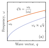
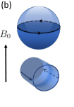
Figure 1: (a) Dispersion of MP waves in the absence (blue dashed) or presence (solid red) of a magnetic field. In the latter case, the spectrum is not only gapped at the Larmor frequency $\omega_{0}$, but is also characterized by the topological Chern number $\mathcal{C}h=\omega_{0}/|\omega_{0}|$. (b) In the presence of a uniform magnetic field, a 2D electron gas confined at the surface of a sphere or a cylinder supports MP waves trapped along the equator or at opposite facets.

Hydrodynamic equations govern not only ocean and atmospheric waves, but also plasma waves. The latter are supported by an electron gas and represent coupled oscillations in the electron density and electric field. Moreover, equations describing plasma waves in a two-dimensional (2D) electron gas on the top of the extended gate (e.g., in field-effect transistors) can be mapped Dyakonov and Shur (1993); Chaplik (1972) to shallow water hydrodynamics, which are usually employed to describe equatorial waves trapped by Earth Matsuno (1966); Delplace et al. (2017). The role of the Coriolis force is played by the Lorentz force due to the external magnetic field. The magnetic field opens a gap in the spectrum of magnetoplasma (MP) waves , as shown in Fig. 1-a, which results in a nontrivial topology  Jin et al. (2016).

Motivated by these observations, we consider plasma oscillations supported by a 2D electron gas confined at the surface of a sphere or cylinder. We argue that in the presence of a uniform magnetic field, these systems host equatorial MP waves. These waves are illustrated in Fig. 1-b and are the counterpart of ocean waves trapped by Earth. We investigate the dependence of their spectrum on the sphere and cylinder radius. For a spherical geometry, the spectrum of equatorial MP waves is sensitive to finite-size effects and is well developed only if the sphere radius exceeds the penetration length for the equatorial MP waves. For a cylindrical geometry, the spectrum of equatorial modes is weakly dependent on the cylinder radius and the overcomes finite-size effects. We argue that the exceptional robustness of this spectrum can be explained by destructive interference between interfacet couplings across the top and bottom hemicylinders. We discuss possible experimental setups, including grains and rods composed of topological insulators (e.g., $\hbox{Bi}_{2}\hbox{Se}_{3}$) or metal-coated dielectrics (e.g., $\hbox{Au}_{2}\hbox{S}$).

The remainder of this paper is organized as follows. In Sec. II, we discuss the primary equations describing MP waves supported by a 2D electron gas in a magnetic field. In Sec. III, we reconsider edge MP modes localized at the domain wall, where the magnetic field switches its sign. Sec. IV is devoted to equatorial MP modes in spherical and cylindrical geometries. Sec. V presents discussions and conclusions.

II II. Magnetoplasma waves

The long-wavelength behavior of MP waves supported by a 2D electron gas can be described with the help of classical hydrodynamic equations Fetter (1985). After linearization, equations for electron density $\rho_{t\mathbf{r}}$ and electric current $\mathbf{j}_{t\mathbf{r}}$ can be presented as

$$\partial_{t}\rho(\mathbf{r},t)+\mathbf{\nabla}\cdot\mathbf{j}(\mathbf{r},t)=0,$$ (1)

$$\partial_{t}\mathbf{j}(\mathbf{r},t)=\frac{ne^{2}}{m}\mathbf{E}(\mathbf{r},t)+\frac{e}{mc}[\mathbf{j}(\mathbf{r},t)\times\mathbf{B}(\mathbf{r})].$$ (2)

Here, $m$ is the cyclotron electron mass . The electric field $E(\mathbf{r},t)=-\nabla\phi(\mathbf{r},t)$ is not external, but is created by electron density oscillations and is treated in a self-consistent manner. The corresponding scalar potential $\phi(\mathbf{r},t)$ is given by

$$\phi(\mathbf{r},t)=\int d\mathbf{r}^{\prime}V(\mathbf{r}-\mathbf{r}^{\prime})\rho(\mathbf{r}^{\prime},t),\quad\;V(\mathbf{q})=\frac{2\pi}{q\kappa(\mathbf{q})},$$ (3)

where $V(\mathbf{r}-\mathbf{r}^{\prime})$ represents interparticle interactions and $V(\mathbf{q})$ gives the corresponding Fourier transform. Here, $\kappa(\mathbf{q})$ is the dielectric function of the medium surrounding the 2D electron gas. Its explicit wave vector dependence for experimentally relevant setups is specified below. The system of equations, Eqs. (1-3), is valid for 2D electrons confined at the surface of an arbitrary geometry. However, it is instructive to start with a discussion of the spectrum and its topology for MP waves in a planar geometry.

A key component to the topological classification of MP waves is the transformation reported in Ref. Jin et al. (2016), which recasts the system of equations, Eqs. (1) - (3), into a Hermitian-Schrödinger-like eigenvalue problem, $\omega\psi(\mathbf{q},\omega)=\hat{H}(\mathbf{q})\psi(\mathbf{q},\omega)$. Here, we have performed the Fourier transform and have introduced $\psi(\mathbf{q},\omega)=\{j^{+}(\mathbf{q},\omega),j^{0}(\mathbf{q},\omega),j^{-}(\mathbf{q},\omega)\}$ with $j^{\pm}(\mathbf{q},\omega)=(j^{x}(\mathbf{q},\omega)\pm ij^{y}(\mathbf{q},\omega))/\sqrt{2}$ and $j^{0}(\mathbf{q},\omega)=\omega_{\mathrm{p}}(\mathbf{q})\rho(\mathbf{q},\omega)/q$. The resulting effective Hamiltonian $H(\mathbf{q})$ for the MP problem is given by

$$\hat{H}(\mathbf{q})=\begin{pmatrix}\omega_{0}&\frac{\omega_{\mathrm{p}}(\mathbf{q})e^{i\phi_{\mathbf{q}}}}{\sqrt{2}}&0\\ \frac{\omega_{\mathrm{p}}(\mathbf{q})e^{-i\phi_{\mathbf{q}}}}{\sqrt{2}}&0&\frac{\omega_{\mathrm{p}}(\mathbf{q})e^{i\phi_{\mathbf{q}}}}{\sqrt{2}}\\ 0&\frac{\omega_{\mathrm{p}}(\mathbf{q})e^{-i\phi_{\mathbf{q}}}}{\sqrt{2}}&-\omega_{0}\\ \end{pmatrix}.$$ (4)

Here, $\phi_{\mathbf{q}}$ is the polar angle for a wave vector $\mathbf{q}$, $\omega_{0}=eB_{0}/mc$ is the Larmor frequency for electrons in a uniform magnetic field $B_{0}$, and $\omega_{\mathrm{p}}(\mathbf{q})=\sqrt{2\pi ne^{2}q/m\kappa(\mathbf{q})}$ is the dispersion for plasma waves in the absence of a magnetic field. The classical nature of the underlying problem manifests in the presence of a particle-hole symmetry, $CH(\mathbf{q})C^{-1}=-H(-\mathbf{q})$ . The states connected by the transformation $C$ have opposite frequencies and are not independent. In addition, the symmetry guarantees that any observables (e.g., $\rho(\mathbf{r},t)$ or $j(\mathbf{r},t)$ are real numbers. The eigenvalues of the Hamilton $H(\mathbf{q})$ are given by

$$\Omega^{\pm}(\mathbf{q})=\pm\Omega(\mathbf{q}),\quad\hbox{and}\quad\Omega^{0}(\mathbf{q})=0.$$ (5)

The positive-frequency branch $\Omega(\mathbf{q})=\sqrt{\omega_{0}^{2}+\omega_{\mathrm{p}}^{2}(\mathbf{q})}$ governs the dispersion relation for MP waves, as presented in Fig 1-a. In the presence of a magnetic field, the dispersion acquires the gap given by the Larmor frequency $\omega_{0}$. The negative-frequency branch is connected to the positive branch by the particle-hole symmetry transformation and is not dynamically independent. The interplay of the inversion ($\Omega^{0}(-\mathbf{q})=\Omega^{0}(\mathbf{q})$) and particle-hole ($\Omega^{0}(-\mathbf{q})=-\Omega^{0}(\mathbf{q})$) symmetries dictates that $\Omega^{0}(\mathbf{q})=0$, which causes the zero-energy branch to be spurious.

By recasting the equations, Eqs. (1- 3), as a Hermitian eigenvalue problem, the topology of the MP spectrum can be classified Jin et al. (2016). Because $H(\mathbf{q})$ belongs to the D-class Ryu et al. (2010), each branch can be characterized by the Chern number as $\mathcal{C}h_{\pm}=\mathrm{sgn}[\omega_{0}]$ with $\mathcal{C}h_{0}=0$. The nontrivial topology can be tracked by presenting the effective Hamiltonian $H(\mathbf{q})$ as $H(\mathbf{q})=\mathbf{h}(\mathbf{q})\cdot\bm{\sigma}$, where $\bm{\sigma}$ is a spin-1 generalization of the Pauli matrix set  and $h(\mathbf{q})=\{\omega_{\mathrm{p}}(\mathbf{q})\cos\phi_{\mathbf{q}},-\omega_{\mathrm{p}}(\mathbf{q})\sin\phi_{\mathbf{q}},\omega_{0}\}$. The unit vector $n(\mathbf{q})=\mathbf{h}(\mathbf{q})/h(\mathbf{q})$ follows the meron-like texture and spans half of the Bloch sphere. In practice, the vector points up ($\omega_{0}>0$) or down ($\omega_{0}<0$) at $\mathbf{q}\rightarrow 0$ and has a vortex-like in-plane texture at $\mathbf{q}\rightarrow\infty$. The topology of the MP wave spectrum is insensitive to the details of screening by external media encoded in $\kappa(\mathbf{q})$, but the latter shapes the dispersion of MP waves.

For a 2D electron gas embedded in dielectric media (e.g., at the interface between air and an insulating substrate), the dielectric function can be approximated as the wave-vector-independent $\kappa$. The resulting dispersion of plasma waves in the absence of an external magnetic field shows a square-root dependence, $\omega_{\mathrm{p}}(\mathbf{q})\propto\sqrt{q}$, which reflects the nonlocal nature of long-range Coulomb interactions . Once it is transformed to real space, the square-root dispersion does not have any local representation in terms of $\nabla_{\mathbf{r}}$, which complicates analytical treatments for MP edge states. For a 2D electron gas placed at a distance $L$ from an extended gate, the charge carriers in the gate actively participate in screening interactions. The corresponding wave vector dependence of the dielectric constant can be approximated as $\kappa(\mathbf{q})=\kappa/\tanh{qL}$ Fetter (1985). The long-range nature of the interactions is lost, and the plasma wave dispersion $\omega_{\mathrm{p}}(\mathbf{q})=\sqrt{2\pi ne^{2}q\;\mathrm{th}(qL)/m\kappa}$ becomes linear $\omega_{\mathrm{p}}(\mathbf{q})\approx uq$ at long wavelengths, $qL\lesssim 1$. Here, $u=\sqrt{2\pi ne^{2}L/m\kappa}$ is the corresponding plasma wave velocity. The effective Hamiltonian $H_{\mathbf{q}}$ is simplified as

$$\hat{H}^{\prime}(\mathbf{q})=\begin{pmatrix}\omega_{0}&\frac{u(q_{x}+iq_{y})}{\sqrt{2}}&0\\ \frac{u(q_{x}-iq_{y})}{\sqrt{2}}&0&\frac{u(q_{x}+iq_{y})}{\sqrt{2}}\\ 0&\frac{u(q_{x}-iq_{y})}{\sqrt{2}}&-\omega_{0}\\ \end{pmatrix}$$ (6)

and can be transformed in real space in a straightforward manner. It should be mentioned that in this approximation, there is a one-to-one mapping between plasma waves and surface waves within the shallow-water hydrodynamics usually used for describing equatorial ocean waves trapped by Earth Delplace et al. (2017).

The nontrivial topology of the bulk MP wave spectrum dictates the presence of edge MP modes localized at sample boundaries or domain walls, where the magnetic field flips its sign. Before addressing the equatorial MP waves in spherical and cylindrical geometries, which are the focus of Sec. IV, we reconsider the domain wall problem in planar geometry and demonstrate that the spectrum of edge MP modes is more complicated than was previously reported Jin et al. (2016).

III III. Domain walls in planar geometry

According to the bulk-edge correspondence, the magnetic field domain wall is expected to host a pair of chiral states propagating in only one direction. The domain wall problem has already been considered in Ref. [Jin et al., 2016], in which the plasma wave spectrum is assumed to be linear (interactions are overscreened) and a step-like ansatz $b(x)=B_{0}\hbox{sgn}[x]$ is employed for the magnetic field profile. With these approximations, the spectrum includes bulk bands given by Eq. (5) as edge MP modes. The positive-frequency region of the spectrum for edge MP waves is given by

$$\Omega^{\mathrm{I}}(k)=-uk,\quad\quad\Omega^{\mathrm{II}}(k)=\omega_{0}\quad\hbox{at}\quad k>0.$$ (7)

Here, $k$ is the wave vector along the domain wall. The first mode $\Omega^{\mathrm{I}}(k)$ is chiral and connects the positive and zero-frequency branches, but this is not the case for the second mode $\Omega^{\mathrm{II}}(k)$. This unusual behavior can be regularized by introducing transverse viscosity into the hydrodynamic equations Tauber et al. (2020). However, it has been further discovered that the spectrum is sensitive to boundary conditions at the domain wall and to the regularization scheme, which can be referred to as an anomalous bulk- or interface-boundary correspondence Tauber et al. (2020); Graf et al. (2021); Tauber and Thiang (2021); Faure (2019); Tauber et al. (2019); Fu and Qin (2021).

In the present paper, we reconsider the domain wall problem. We demonstrate that the edge MP wave spectrum admits an analytical solution for the smooth ansatz $B(x)=B_{0}b(x)$ with $b(x)=\tanh(x/d)$. Here, $d$ is the domain wall width. We start with the exclusion of $j^{0}(\mathbf{r},t)$ and incorporate translational symmetry along the domain wall. The latter allows us to search for solutions in the following form:

$$\begin{split}\mathbf{j}^{x(y)}(\mathbf{r},t)=J^{x(y)}(x)e^{i(ky-\omega t)},\\ j^{0}(\mathbf{r},t)=J^{0}(x)e^{i(ky-\omega t)}.\end{split}$$ (8)

As a result, $J^{x(y)}\equiv J^{x(y)}(x)$ satisfy the following set of equations:

$$\begin{split}(\omega^{2}+u^{2}\partial_{x}^{2})J^{x}=-i(u^{2}k\partial_{x}-\omega_{0}\omega b(x))J^{y},\\ (\omega^{2}-u^{2}k^{2})J^{y}=-i(u^{2}k\partial_{x}+\omega_{0}\omega b(x))J^{x}.\end{split}$$ (9)

As clearly shown, these equations admit a pair of solutions:

$$\quad J^{x}=0,\quad\quad J^{y}\sim\exp\left[\pm\frac{\omega_{0}}{u}\int_{0}^{x}dx^{\prime}b(x^{\prime})\right]$$ (10)

with the dispersion $\Omega_{\mathrm{K}}^{\pm}(k)=\pm uk$. For the considered ansatz $b(x)=\tanh(x/d)$, only mode $\Omega_{\mathrm{K}}^{-}(k)=-uk$ can be properly normalized and matches with $\Omega^{\mathrm{I}}(k)$ given by Eq. (7). If we follow the terminology for equatorial waves, the mode $\Omega_{\mathrm{K}}(k)\equiv\Omega_{\mathrm{K}}^{-}(k)$ can be referred to as the Kelvin MP mode. Importantly, its dispersion does not depend on the details of the domain wall profile; rather, it is only required that the latter has a kink . As a longitudinal edge wave ($J^{x}=0$), the Kelvin mode is accompanied by density oscillations with the same profile $J^{0}=-J^{y}$ as for $J^{y}$. For the employed ansatz $b(x)$, the profile is symmetric, $J^{y}\propto 1/[\cosh\left(x/d\right)]^{\omega_{0}d/v}$, across the domain wall.

If $\omega^{2}\neq u^{2}q^{2}$, the set of equations in Eq. (9) can be combined in a single equation given by

$$-u^{2}\partial_{x}^{2}J^{x}+\left[u^{2}k^{2}+\omega_{0}^{2}b^{2}(x)-\omega^{2}-\frac{u^{2}k\omega_{0}}{\omega}\partial_{x}b(x)\right]J^{x}=0.$$

If we incorporate the explicit expression for the domain wall profile $b(x)=\tanh(x/d)$ and re-scale the coordinate $x\rightarrow x/d$, this eigenvalue problem transforms into a one-dimensional quantum mechanical problem with the P$\ddot{o}$schl–Teller (PT) confining potential, which is given by

$$-\partial_{x}^{2}J^{x}-\frac{\lambda(\lambda+1)}{\cosh^{2}x}J^{x}=\epsilon J^{x}.$$ (11)

The parameter $\lambda$ and eigenenergy $\epsilon$ depend on both the wave vector $k$ and frequency $\omega$ and are given by

$$\begin{split}\lambda(\lambda+1)=\frac{\omega_{0}}{\omega_{\mathrm{d}}}\frac{uk}{\omega}+\frac{\omega^{2}_{0}}{\omega_{\mathrm{d}}^{2}},\quad\;\epsilon=\frac{\omega^{2}-u^{2}k^{2}-\omega_{0}^{2}}{\omega_{\mathrm{d}}^{2}}.\end{split}$$ (12)

Here, $\omega_{\mathrm{d}}=u/d$ is the frequency scale determined by the domain wall width. The PT potential belongs to the class of supersymmetric potentials Cooper et al. (1995); Çevik et al. (2016). Its spectrum has been extensively studied and is known to admit an analytical solution. The spectrum includes a continuum of extended states and a set of discrete states given by

continuous: $$\epsilon>0,$$ (13)

discrete: $$\epsilon_{n}=-(\lambda-n)^{2}, \quad n\leq\lambda.$$ (14)

The continuous region $\epsilon>0$ determines the continuum of bulk MP states with frequencies $\omega^{2}=\omega_{0}^{2}+v^{2}k^{2}+\epsilon\omega_{\mathrm{d}}^{2}$. The discrete bound states of the PT problem are intricately related to the MP edge modes trapped at the domain wall. The dispersion relation for edge MP waves satisfies the following equation, which can be obtained if we combine Eqs. (12) and (14):

$$\begin{split}\omega^{2}-(uk)^{2}+\omega_{0}\omega_{\mathrm{d}}\Big{[}\frac{uk}{\omega}-\\ \frac{\sqrt{\omega_{0}^{2}+u^{2}k^{2}-\omega^{2}}}{\omega_{0}}(2n+1)-\frac{\omega_{\mathrm{d}}}{\omega_{0}}n(n+1)\Big{]}=0.\end{split}$$ (15)

Due to its nonlinear nature, the equation can have multiple solutions for given $n=0,1,...$ and $k$. In dimensionless units $\omega/\omega_{0}$ and $k/k_{0}$ with $k_{0}=\omega_{0}/u$, the edge MP wave spectrum depends only on the parameter $\alpha=\omega_{\mathrm{d}}/\omega_{0}$. The spectrum for smooth ($\alpha=0.2$) and sharp ($\alpha=5$) domain wall profiles is presented in Fig. 2. If we follow the terminology for equatorial waves, the resulting MP edge modes can be labeled as Yanai, Poincaré, and Rossby modes. It is instructive to briefly discuss these modes separately.

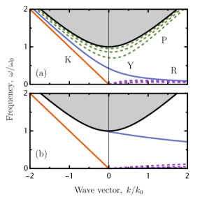
Figure 2: Spectrum for edge MP waves trapped by magnetic field domain walls with smooth ((a) $\alpha=0.2$) and sharp ((b) $\alpha=5$) profiles. The spectrum includes chiral and protected Kelvin (K) and Yanai (Y) modes coexisting with topologically trivial Rossby (R) and Poincaré (P) modes. The shaded area denotes the continuum of bulk extended states.

Yanai mode. This mode is chiral and connects the bulk state continuum with zero-frequency states. The stability of the Yanai mode is intricately related to the fact that it originates from the ground bound state ($n=0$) for the PT problem . Therefore, the profile of transverse current oscillations within the Yanai mode is symmetric and is given by $J^{x}\propto 1/[\cosh\left(x/d\right)]^{\lambda}$. However, the profiles for the longitudinal current and density oscillations are antisymmetric across the domain wall, $J^{y},J^{0}\propto b(x)J^{x}$, which ensures that wave functions for Kelvin and Yanai waves are orthogonal to each other. Their cumbersome expressions are presented in Appendix A.

Poincaré modes. The Poincaré modes are trivial edge modes propagating in both directions along the domain wall. Poincaré modes originate from the excited bound states for the PT problem and are therefore labeled by the discrete index $n=1,2,3,...$. These states appear only if the domain wall is sufficiently smooth. Their number can be counted as $N_{\mathrm{P}}=\lfloor(\sqrt{1+4\omega_{0}^{2}/\omega_{\mathrm{d}}^{2}}-1)/2\rfloor$, and the first Poincaré mode splits from the bulk continuum at $\alpha=1/\sqrt{2}$ .

Rossby modes. These low-energy modes result from the reshaping of zero-frequency bulk states . The Rossby modes also originate from the excited bound states for the PT problem and are therefore labeled by the discrete index $n=1,2,3,...$, similar to the Poincaré modes. The dispersion of the Rossby modes is well approximated by

$$\Omega_{\mathrm{R}}^{n}(k)\approx\frac{uk\omega_{\mathrm{d}}}{u^{2}k^{2}+\omega_{\mathrm{d}}\sqrt{\omega_{0}^{2}+u^{2}k^{2}}(2n+1)+\omega_{\mathrm{d}}^{2}n(n+1)}$$

and reaches a maximum at intermediate wave vectors for which the group velocity $\partial_{k}\Omega_{\mathrm{R}}^{n}(k)$ flips its sign. For this reason, these modes also propagate in both directions along the domain wall. The slowly varying spatial profile of the magnetic field is an important ingredient for the formation of Rossby MP modes. To the best of our knowledge, these modes have been previously overlooked in condensed matter setups. However, they have been well documented in stellar magnetohydrodynamics as well as in ocean and atmosphere hydrodynamics (see Ref. Zaqarashvili et al. (2021) and references therein for a review).

The presence of chiral Kelvin and Yanai modes is in agreement with the bulk-boundary correspondence, which dictates the presence of two topologically protected modes. Our calculations have clearly demonstrated that the unusual behavior of the spectrum, Eq. (7), and the anomalous bulk-edge correspondence are artifacts of the step-like ansatz for the magnetic domain wall profile.

It is instructive to consider the limit toward the domain wall with a step-like profile, $d\rightarrow 0$ (or $\alpha\rightarrow\infty$). In this limit, there are no Poincaré modes. The dispersion for the Kelvin mode is $\alpha$-independent, but the behavior of the Yanai and Rossby modes is quite sensitive. For small wave vectors, $k\lesssim\alpha^{-1}$, the dispersion curves become flattened, $\Omega_{\mathrm{R}}^{n}(k)\approx 0$ and $\Omega_{\mathrm{Y}}(k)\approx\omega_{0}$, mimicking the spectrum, Eq. (7), derived for the step-like profile. However, for large wave vectors, $k\gtrsim\alpha^{-1}$, both modes become dispersive and deviate from Eq. (7). The lack of a smooth transition in the limit $d\rightarrow 0$ can be seen as another signature of the anomalous bulk-boundary correspondence.

The derivation presented above for the spectrum of edge MP modes assumes that that Coulomb interactions are overscreened. However, the classification of edge modes is generic and does not rely on the details of screening provided by external media. We will use this classification in the next section, in which spherical and cylindrical geometries are considered.

IV IV. Spherical and cylindrical geometries

The system of equations describing MP waves is valid for a 2D electron gas confined at the surface of an arbitrary geometry. Only the magnetic field component perpendicular to the surface influences the dynamics of electrons via the Lorentz force, which naturally becomes position-dependent for a curved surface. For a sphere or cylinder penetrated by a uniform magnetic field $B_{0}$, the radial component has a profile of $B_{\mathrm{R}}(\mathbf{r})=B_{0}\cos(\theta)$, where $\theta$ is the corresponding polar angle. The radial component $B_{\mathrm{R}}(\mathbf{r})$ vanishes and changes sign along the equator or at two facets, where the presence of equatorial MP modes is anticipated.

This setup can be naturally realized in grains and rods composed of a topological insulator (e.g., $\hbox{Bi}_{2}\hbox{Se}_{3}$) that exhibit insulating bulk behavior  and have topologically protected surface states. A fabrication of micron- and submicron-sized grains and rods have already been reported Campos et al. (2018); Hamdou et al. (2013); Cho et al. (2015); Münning et al. (2021); Kunakova et al. (2018); Ziegler et al. (2018); Jauregui et al. (2015); Dufouleur et al. (2017). The topological surface states are described by the relativistic-like Dirac equation, and their dispersion is linear $\epsilon_{\mathbf{p}}=vp$ with velocity $v$. The bulk MP waves in $\hbox{Bi}_{2}\hbox{Se}_{3}$ thin films have been previously reported Autore et al. (2015), and we use a corresponding set of parameters. Here, we apply the Dirac velocity $v=0.67\;10^{6}\;\hbox{cm}^{-2}$, electron density $n\approx 7\;10^{12}~{}\hbox{cm}^{-2}$, and magnetic field $B\approx 2\;\hbox{T}$. The corresponding Fermi energy and Larmor frequency are given by $\epsilon_{\mathrm{F}}\approx 0.4\;\hbox{eV}$ and $\hbar\omega_{0}\approx 1.2\;\hbox{meV}$, respectively. Due to the absence of an external gate induced extra screening, the effective dielectric constant $\kappa=35$ for a $\hbox{Bi}_{2}\hbox{Se}_{3}$-air interface can be approximated to be wave vector independent. The screening impacts only the strength of the Coulomb interactions and their long-range nature is retained.

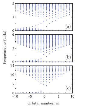
Figure 3: Spectrum of MP waves supported by a 2D electron gas confined at the surface of a sphere with radius $100\;\mu\hbox{m}$ (a), $10\;\mu\hbox{m}$ (b), or $1\;\mu\hbox{m}$ (c). The equatorial modes are well developed only if the sphere radius exceeds the penetration length $l_{0}\approx 5\;\mu\hbox{m}$.

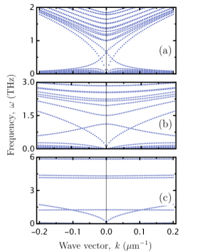
Figure 4: Spectrum of MP waves supported by a 2D electron gas confined at the surface of a cylinder with radius $100\;\mu\hbox{m}$ (a), $10\;\mu\hbox{m}$ (b), or $1\;\mu\hbox{m}$ (c). The chiral Kelvin and Yanai modes demonstrate exceptional robustness and are well developed even if the cylinder radius is smaller than the penetration length $l_{0}\approx 5\;\mu\hbox{m}$. As we discuss in the main text, the robustness can be explained by destructive interference between interfacet couplings across the top and bottom hemicylinders.

The classical description of MP waves ignores the discrete nature of the Dirac electron spectrum due to the magnetic field and finite-size effects. The classical approach is justified by the hierarchies of energy scales, $\hbar\omega_{0}\ll\epsilon_{\mathrm{F}}$ and $\hbar\omega_{\mathrm{R}}^{\mathrm{e}}\ll\epsilon_{\mathrm{F}}$, where $\omega_{\mathrm{R}}^{\mathrm{e}}=v/\mathrm{R}$. These relations are well satisfied for the considered range of magnetic fields and for the $\mu$m-sized samples considered below. Another important length scale is the penetration length $l_{0}$ for edge MP waves. This scale can be estimated as the inverse wave vector $l_{0}=q^{-1}$ at which $\omega_{\mathrm{P}}(q)=\omega_{0}$. Here $\omega_{\mathrm{P}}(q)=\sqrt{2\pi ne^{2}q\;/m\kappa}$ is dispersion of plasma waves in the absence of magnetic field and the external screening. For the considered set of parameters, we have $l_{0}\approx 5~{}\mu\hbox{m}$. For grains and rods with radius $R\sim l_{0}$, the finite-size effects become essential. It is instructive to discuss the spherical and cylindrical geometries separately.

For a spherical geometry, the system of equations describing MP waves, Eqs. (1) - (3), can be solved via an expansion over the vector spherical harmonics. These calculations are presented in Appendix B. The spherical harmonics are labeled by the orbital discrete numbers $l=0,1,2,...$ and $m=-l,...,l$. In the presence of a uniform magnetic field, the axial symmetry remains, indicating that $m$ is still a good discrete number. The evaluated spectrum is presented in Fig. 3, which displays results for a sphere with radius $100\;\mu\hbox{m}$ (a), $10\;\mu\hbox{m}$ (b), or $1\;\mu\hbox{m}$ (c). For $R\gg l_{0}$, the spectrum of Kelvin, Yanai, and Rossby waves is well developed, resembling the spectrum calculated for the planar geometry with overscreened interactions in Sec. III. However, in this case, the topological Kelvin MP wave exhibits square-root behavior instead of linear behavior. The discrete nature of the spectrum can be attributed to the formation of standing waves that restrict the wave vector along the equator $k_{\mathrm{\phi}}$ as $k_{\mathrm{\phi}}R=m$. The Poincaré modes become indistinguishable from the discrete modes originating from the bulk continuum. When the radius becomes comparable to the penetration length $R\lesssim l_{0}$, the equatorial modes are pushed outside the gap and are no longer well resolved.

For a cylindrical geometry, the system of equations describing MP waves, Eqs. (1) - (3), can be solved via a Fourier transform and an expansion over the circular harmonics. Due to the translational symmetry along the cylinder, the spectrum can be labeled by the corresponding wave vector $k$, as presented in Fig. 4. We have used the same values for the cylinder radius: $100\;\mu\hbox{m}$ (a), $10\;\mu\hbox{m}$ (b), and $1\;\mu\hbox{m}$ (c). For $R\gg l_{0}$, the spectrum represents superimposed independent spectra for two domain walls that are situated at the opposite facets of the cylinder, as illustrated in Fig. 1-b. When the radius becomes comparable to the penetration length $R\lesssim l_{0}$, indistinguishable discrete bulk and Poincaré modes are pushed outside the gap, while the Rossby modes are shifted toward larger wave vectors. The Yanai modes from different facets experience the hybridization that is the most prominent in the vicinity of their avoided crossing at $k=0$. However, this behavior is not observed for the Kelvin and Yanai waves. At first glance, their exceptional robustness and ability to overcome finite-size effects are surprising. The dispersion curves for the Kelvin and Yanai modes from opposite facets intersect. As a result, any overlap between them is expected to induce intermode hybridization and a gap between the hybrid modes. We attribute their robustness to these destructive interference effects. Because the Kelvin MP mode is longitudinal ($J^{x}=0$), its hybridization with the Yanai mode from the opposite facet originates from the overlap between transverse current $J^{y}$ and electron density $J^{0}$ components. As presented in Appendix A, the profiles across the domain wall are symmetric for the Kelvin mode, but antisymmetric for the Yanai mode. As a result, the overlapping regions in the top and bottom hemicylinders have opposite signs but the same magnitude; thus, their total contribution vanishes. In other words, the couplings across the top and bottom hemicylinders interfere destructively, which forbids intermode hybridization and ensures exceptional robustness of the equatorial MP mode spectrum in the cylindrical geometry. We discuss the robustness of spectra and destructive interference effects in detail in Appendix A.

V V. Discussion

In our description of MP waves, we have neglected retardation effects for the electric field. These effects are of second order for the factor $\omega_{0}/kc$. This factor is very small in the full wave vector range, except for vanishingly small momenta, $k\lesssim\omega_{0}/c$ . We have also omitted the time-dependent magnetic field created by density oscillations in electron gas, which can also be treated in a self-consistent manner. This magnetic field impacts only nonlinear dynamics of MP waves. In addition, the transverse electric field generated by magnetic field oscillations is also of the second order for the small factor $\omega_{0}/kc$ and can be safely neglected.

The hydrodynamic description of magnetoplasma waves neglects effects of the spatial dispersion in the response of the electron gas. These effects are of little importance in a wide frequency range (including the range corresponding to equatorial magnetoplasma waves), but are essential in the vicinity of overtones, $n_{\mathrm{B}}\omega_{0}$ with integer $n_{\mathrm{B}}$, for the cyclotron frequency. Effects of the spatial dispersion allow the hybridization between cyclotron resonance overtones and magnetoplasma waves that results in a formation of Bernstein modes Bernstein (1958); Chiu and Quinn (1974); Volkov and Zabolotnykh (2014); Roldán et al. (2011). The latter have been observed as in conventional conventional GaAs/AlGaAs heterostructures Batke et al. (1985, 1986); Holland et al. (2004); Richards (2000) as in graphene Bandurin et al. (2022).

Edge MP waves localized at sample edges (including edge states in arrays of metallic disks or ribbons) have been extensively studied in conventional GaAs/AlGaAs heterostructures Allen et al. (1983), graphene Kumada et al. (2014); Crassee et al. (2012); Yan et al. (2012), and topological insulators Autore et al. (2015). In contrast, magnetic field domain wall MP states have been reported only very recently in a circular-shaped domain wall imprinted in a GaAs/AlGaAs heterostructure Jin et al. (2019). These states have been effectively probed via near-field radiation. However, due to the narrow frequency resolution of corresponding waveguides, only Kelvin MP waves have been reported. This approach, as well as other near-field radiation approaches, can be employed to detect equatorial MP waves.

Due to the discrete nature of their spectrum, equatorial MP waves in the spherical geometry can also be optically probed (far-field regime). In the dipole approximation, only modes with $m=\pm 1$ are optically active, which can be seen as the selection rules for MP waves. Symmetry analysis demonstrates that the equatorial modes with higher $m$ values can be excited via optical vortex beams. It has already been demonstrated that these beams can resonantly couple with quadrupole and hexapole plasma modes in metallic nanostructures (e.g., discs) Tan et al. (2008); Sakai et al. (2015), and we anticipate that they can be used to resonantly excite equatorial MP waves. Alternatively, equatorial MP waves can be probed via scattering of light by the grain. The corresponding theory of Mie scattering has already been extended to grains and rods made of topological insulators Ge et al. (2015, 2015); Lakhtakia and Mackay (2016); Schultz et al. (2020), but in the absence of external an uniform magnetic field, which is an essential ingredient for the formation of equatorial MPs. The magnetic field breaks the spherical symmetry that is the cornerstone assumption of the Mie theory, and its extension is beyond the scope of the present work.

The employed classical description of MP waves is justified by the hierarchy of energy scales, $\hbar\omega_{\mathrm{R}}^{\mathrm{e}}\ll\epsilon_{\mathrm{F}}$, which is well satisfied for the $\mu$m-sized samples considered in this work. It should be mentioned that nm-sized topological insulator structures have previously attracted much attention Imura et al. (2011); Governale et al. (2020); Imura et al. (2012); Gioia et al. (2019); Siroki et al. (2016) because the curved nature of the grain or rod surface results in the spin Berry phase for Dirac electrons. The latter can be described by the effective vector potential associated with a fictitious magnetic monopole induced at the center of the grain Imura et al. (2012); Gioia et al. (2019); Siroki et al. (2016) or a magnetic flux penetrating the rod Imura et al. (2011); Governale et al. (2020). Via the Aharonov-Bohm effect, these systems exhibit a shift in the single-particle spectrum for Dirac electrons. These effects cannot be captured by the classical approach, but are only important for nm-sized samples.

Grain and rods composed of a topological insulator (e.g., $\hbox{Bi}_{2}\hbox{Se}_{3}$ or $\hbox{Bi}_{2}\hbox{Te}_{3}$) represent a promising setup for experimental observation of equatorial MP waves. However, the unconventional physics of Dirac surface states, which are also manifested in plasmonics Raghu et al. (2010); Efimkin et al. (2012a, b); Stauber et al. (2013); Efimkin and Kargarian (2021); Lai et al. (2014), are of little importance. Another possible setup involves conventional metal-coated dielectric particles (e.g., $\hbox{Au}_{2}\hbox{S}$  Averitt et al. (1997); Daneshfar and Bazyari (2014); Perera et al. (2020)). While spherical and cylindrical geometries are convenient for theoretical analysis, the topological nature of equatorial MP waves guarantees their presence for any closed conducting surface penetrated by a uniform magnetic field.

We have demonstrated that the domain wall, where the magnetic field is smooth and switches its sign, hosts four distinct MP waves, including Kelvin, Yanai, Rossby, and Poincaré modes. It should be noted that MP edge modes of a different physical origin can be hosted at domain walls separating regions with different electron densities Mikhailov and Volkov (1992); Aleiner and Glazman (1994); Xia and Quinn (1994) or the anomalous Hall conductivities Song and Rudner (2016); Petrov (2021), as well as at edges of anisotropic two-dimensional materials Sokolik et al. (2021).

To conclude, we have considered plasma oscillations supported by a 2D electron gas confined at the surface of a sphere or cylinder. We argue that in the presence of a uniform magnetic field, these systems host a set of equatorial MP waves that represent counterparts to the equatorial waves trapped by Earth due to its rotation.

VI Acknowledgements

We acknowledge support from the Australian Research Council Centre of Excellence in Future Low-Energy Electronics Technologies.

Appendix A APPENDIX A. Robustness of equatorial MP modes in the cylindrical geometry

A.1 A1. Wave functions for Kelvin and Yanai modes

Wave functions for Kelvin and Yanai MP modes can be directly calculated from the Hermitian eigenvalue problem defined in Eq. (6). If we use the following ansatz:

$$\mathbf{j}^{x(y)}({\mathbf{r},t})=J^{x(y)}(x)e^{i(ky-\omega t)},\quad\quad\quad\mathbf{j}^{0}({\mathbf{r},t})=J^{0}(x)e^{i(ky-\omega t)},$$ (16)

the eigenvalue problem can be presented as

$$-i\omega J^{x} =-u\partial_{x}J^{0}+\omega_{0}b(x)J^{y},$$ (17)

$$-i\omega J^{0} =-u\partial_{x}J^{x}-iukJ^{y},$$ (18)

$$-i\omega J^{y} =-iukJ^{0}-\omega_{0}b(x)J^{x}.$$ (19)

The Kelvin mode is longitudinal $J^{x}=0$, the transverse current profile is given by Eq. (10), and the resulting density oscillation profile is equal to $J^{0}=-J^{y}$. If we incorporate the explicit expression for the domain wall profile $b(x)=\tanh(x/d)$, the wave function for the Kelvin mode (up to a normalization factor) can be presented as

$$\psi_{\mathrm{K}}\propto\begin{pmatrix}-\frac{i}{\sqrt{2}}\\ 1\\ \frac{i}{\sqrt{2}}\\ \end{pmatrix}\frac{1}{\left[\cosh\left(\frac{x}{d}\right)\right]^{\frac{1}{\alpha}}},$$ (20)

where $\alpha=\omega_{\mathrm{d}}/\omega_{0}$ is the only controlling parameter introduced in the main text. Importantly, the profiles for its nonzero components $J^{y}$ and $J^{0}$ are symmetric across the domain wall.

For the Yanai mode, the transverse current profile is given by $J^{x}\propto 1/[\cosh\left(x/d\right)]^{\lambda}$. Here, $\lambda$ is wave-vector-dependent and must be evaluated from Eq. (12). The longitudinal current and density profiles can be calculated from Eqs. (18) and (19), which results in

$$J^{y}=\frac{i(u^{2}k\partial_{x}+\omega\omega_{0}b(x))J^{x}}{u^{2}k^{2}-\omega^{2}}=\frac{i\omega_{0}(\omega-uk\lambda\alpha)}{u^{2}k^{2}-\omega^{2}}b(x)J^{x}=iA^{y}b(x)J^{x},$$ (21)

$$J^{0}=\frac{i(uk\omega_{0}b(x)+\omega u\partial_{x})J^{x}}{u^{2}k^{2}-\omega^{2}}=\frac{i\omega_{0}(uk-\omega\lambda\alpha)}{u^{2}k^{2}-\omega^{2}}b(x)J^{x}\equiv iA^{0}b(x)J^{x}.$$ (22)

The introduced factors $A^{y}$ and $A^{0}$ can be interpreted as relative amplitudes for the $J^{y}$ and $J^{0}$ profiles with respect to the $J^{x}$ profile. Despite the presence of a singular denominator, the wave vector dependence is smooth. In terms of these amplitudes, the wave function for the Yanai MP mode can be presented as

$$\psi_{\mathrm{Y}}\propto\begin{pmatrix}\frac{1-A^{y}b(x)}{\sqrt{2}}\\ iA^{0}b(x)\\ \frac{1+A^{y}b(x)}{\sqrt{2}}\\ \end{pmatrix}\frac{1}{\left[\cosh\left(\frac{x}{d}\right)\right]^{\lambda}}.$$ (23)

The transverse current profile $J^{x}$ is symmetric across the domain wall, but the $J^{y}$ and $J^{0}$ profiles have antisymmetric shapes. This behavior ensures that Kelvin and Yanai modes hosted by the domain wall are orthogonal to each other, $\langle\psi_{\mathrm{K}}|\psi_{\mathrm{Y}}\rangle=0$. This behavior also plays an important role in the hybridization between equatorial MP modes hosted by opposite facets in the cylinder geometry.

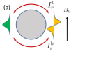
Figure 5: (a) The sketch illustrates the absence of the intermode hybridization due to the destructive interference between couplings across top and bottom hemicyliders. This behavior arises from the fact that the transverse current $J^{y}$ and density $J^{0}$ components are symmetric for the Kelvin mode (green) and antisymmetric for the Yanai mode (yellow). (b) Spectrum for MP waves in the presence of a superimposed circularly symmetric magnetic field $B_{\mathrm{C}}=0.4B_{0}$ with $R=10\;\mu\hbox{m}$. The exact cancellation of intermode hybridization due to destructive interference is lost. Kelvin and Yanai modes from different facets hybridize, and the resulting gap between hybrid modes is the most prominent in the vicinity of the avoided crossings.

A.2 A2. Intermode hybridization and destructive interference effects

For the case of a uniform magnetic field, the component that is perpendicular to the surface, $B^{\mathrm{R}}_{\mathbf{r}}=B_{0}\cos(\theta)$, vanishes at opposite facets of the cylinder. As a result, facets can be seen as a pair of domain walls with opposite profiles (e.g., $b(x)$ and $b(x)^{\prime}=-b(x)$), and the finite-size effects manifest as intermode hybridization. We address the hybridization effects with the help of the analytical model for MP waves introduced in Sec. III of the main paper.

This hybridization is especially important in the vicinity of the intersection ($\omega_{\mathrm{K}}^{\prime}=\omega_{\mathrm{Y}}$ and $\omega_{\mathrm{K}}=\omega_{\mathrm{Y}}^{\prime}$) between dispersion curves for modes hosted at different domain walls. The intersection point can be found analytically, $\omega_{\star}=\omega_{0}\sqrt{\alpha/\alpha+2}$ and $k_{\star}=\omega_{\star}/u$, and the corresponding wave functions for Kelvin and Yanai modes are given by

$$\psi_{\mathrm{K}}^{\prime}\propto\begin{pmatrix}-\frac{i}{\sqrt{2}}\\ -1\\ \frac{i}{\sqrt{2}}\\ \end{pmatrix}\frac{1}{\left[\cosh\left(\frac{x}{d}\right)\right]^{\frac{1}{\alpha}}},\quad\quad\psi_{\mathrm{Y}}\propto\begin{pmatrix}\frac{1-A^{y}_{\star}b(x)}{\sqrt{2}}\\ iA^{0}b(x)\\ \frac{1+A^{y}_{\star}b(x)}{\sqrt{2}}\\ \end{pmatrix}\frac{1}{\left[\cosh\left(\frac{x}{d}\right)\right]^{\frac{1}{\alpha}}},\quad\quad A^{y}_{\star}=-\frac{\alpha+1}{\sqrt{\alpha(\alpha+2)}},\quad A^{0}_{\star}=\frac{1}{\sqrt{\alpha(\alpha+2)}}.$$ (24)

The cylinder surface can be unfolded to a stripe with width $2\pi R$. The problem needs to be supplemented by the periodic boundary conditions and there is a pair of domain walls per period. As discussed below, the closed nature of the geometry is essential. However, it is instructive to begin the analysis with a pair of isolated domain walls.

If we assume that the two domain walls are displaced by $2d_{0}$, the overlap between wave functions for the Kelvin and Yanai modes is given by

$$\langle\psi^{\prime}_{\mathrm{K}}|\psi_{\mathrm{Y}}\rangle=I_{s}\times I_{r},\quad\quad I_{s}=i(A^{y}_{\star}+A^{0}_{\star})=-i\sqrt{\frac{\alpha}{\alpha+2}},\quad I_{r}=N_{\mathrm{K}}N_{\mathrm{Y}}\int_{-\infty}^{\infty}dx\;\frac{1}{\cosh^{\frac{1}{\alpha}}(\frac{x-d_{0}}{d})}\times\frac{\tanh(\frac{x+d_{0}}{d})}{\cosh^{\frac{1}{\alpha}}(\frac{x+d_{0}}{d})}.$$ (25)

Here, $N_{\mathrm{K}}$ and $N_{\mathrm{Y}}$ are normalization factors for the two modes, and their cumbersome explicit expressions are of importance here. The overlap between the Kelvin and Yanai modes is finite. As a result, the hybridization between modes in a system with two domain walls leads to a gap opening and an intersection between dispersion curves.

Due to the closed nature of the cylindrical geometry, the hybridization is mediated across the top and bottom hemispheres. As a result, the overlap integral $I_{r}$ must be modified as $I_{r}\rightarrow I_{r}^{\mathrm{t}}+I_{r}^{\mathrm{b}}$, where $I_{r}^{\mathrm{t}}$ and $I_{r}^{\mathrm{b}}$ are given by

$$I_{r}^{\mathrm{t}}=N_{\mathrm{K}}N_{\mathrm{Y}}\int_{-\pi R}^{0}dx\;\frac{1}{\cosh^{\frac{1}{\alpha}}(\frac{x+\pi R}{d})}\times\frac{\tanh(\frac{x}{d})}{\cosh^{\frac{1}{\alpha}}(\frac{x}{d})},\quad\quad\quad I_{r}^{\mathrm{b}}=N_{\mathrm{K}}N_{\mathrm{Y}}\int_{0}^{\pi R}dx\;\frac{1}{\cosh^{\frac{1}{\alpha}}(\frac{x-\pi R}{d})}\times\frac{\tanh(\frac{x}{d})}{\cosh^{\frac{1}{\alpha}}(\frac{x}{d})}.$$ (26)

These terms have the same magnitudes but opposite signs, causing the total coupling $I_{r}$ to vanish. This behavior arises from the fact that the transverse current $J^{y}$ and density $J^{0}$ components are symmetric for the Kelvin mode and antisymmetric for the Yanai mode. In other words, the couplings across the top and bottom hemicylinders interfere destructively, thus forbidding intermode hybridization. This lack of intermode hybridization ensures the exceptional robustness of equatorial MP modes and their ability to overcome finite-size effects.

A.3 A3. Breaking the destructive interference via an additional circularly symmetric magnetic field

The cancellation of intermode hybridization relies on the symmetry between contributions across the top $I_{r}^{\mathrm{t}}$ and bottom $I_{r}^{\mathrm{b}}$ hemicylinders. If we superimpose uniform $B_{0}$ and circularly symmetric $B_{\mathrm{C}}$ magnetic fields, the corresponding radial component is given by $B_{\mathbf{r}}^{\mathrm{R}}=B_{0}\cos(\theta)+B_{\mathrm{C}}$, and the symmetry between the hemicylinders is broken. The MP wave spectrum evaluated for $B_{\mathrm{C}}=0.4B_{0}$ and $R=10\;\mu\hbox{m}$ (all other parameters are the same as in the main part of the paper) is presented in Fig. 5-b. As anticipated, the Kelvin and Yanai modes from different facets hybridize, and the resulting gap between the hybrid modes is most prominent in the vicinity of the avoided crossings.

Appendix B APPENDIX B. MP waves in the spherical geometry

B.1 B1. Spherical scalar and vector harmonics

For the spherical geometry, the system of integro-differential equations describing MP waves, Eqs. (1) - (3), can be reduced to algebraic equations via decomposition over the spherical vector harmonics. The decomposition is applied as follows:

$$\begin{split}\rho(\mathbf{r},t)=\sum_{n}\rho(n,t)Y_{n}(\mathbf{o}),\quad\quad\mathbf{j}(\mathbf{r},t)=\sum_{n}\left[j^{Y}(n,t)\mathbf{Y}_{n}(\mathbf{o})+j^{\Psi}(n,t)\mathbf{\Psi}_{n}(\mathbf{o})+j^{\Phi}(n,t)\mathbf{\Phi}_{n}(\mathbf{o})\right],\\ \phi(\mathbf{r},t)=\sum_{n}\phi(n,t)Y_{n}(\mathbf{o}),\quad\quad\mathbf{E}(\mathbf{r},t)=\sum_{n}\left[E^{Y}(n,t)\mathbf{Y}_{n}(\mathbf{o})+E^{\Psi}(n,t)\mathbf{\Psi}_{n}(\mathbf{o})+E^{\Phi}(n,t)\mathbf{\Phi}_{n}(\mathbf{o})\right].\end{split}$$ (27)

Here, $\mathbf{r}=\{R\cos\phi\sin\theta,R\sin\phi\sin\theta,R\cos\theta\}$ is the radius vector constrained to the surface of a sphere with radius $R$. For the sake of brevity, we have combined azimuthal $\theta$ and polar $\phi$ angles as $\mathbf{o}=\{\theta,\phi\}$. The index $n=\{l,m\}$ includes two angular discrete numbers, $l=0,1,2,...$ and $m=-l,...,l$. The function $Y_{n}(\mathbf{o})$ is the (scalar) spherical harmonic, which defines the vector spherical harmonics as follows:

$$\mathbf{Y}_{n}(\mathbf{o})=\mathbf{e}_{\mathbf{r}}^{\mathrm{R}}Y_{n}(\mathbf{o}),\quad\quad\mathbf{\Psi}_{n}(\mathbf{o})=\frac{R\mathbf{\nabla}Y_{n}(\mathbf{o})}{\sqrt{l(l+1)}},\quad\quad\mathbf{\Phi}_{n}(\mathbf{o})=\frac{R[\mathbf{e}_{\mathbf{r}}^{\mathrm{R}}\times\mathbf{\nabla}Y_{n}(\mathbf{o})]}{\sqrt{l(l+1)}}.$$ (28)

Here, $\mathbf{e}_{\mathbf{r}}^{\mathrm{R}}$ is the unit vector perpendicular to the surface of the sphere. For each value of $n$, the vector harmonics are orthogonal in the typical three-dimensional manner. In addition, the harmonics form a complete and orthonormal vector set, which is properly normalized as

$$\int d\mathbf{o}\;\mathbf{Y}_{n}^{*}(\mathbf{o})\mathbf{Y}_{n^{\prime}}(\mathbf{o}) =\delta_{nn^{\prime}},\quad\quad\int d\mathbf{o}\;\mathbf{Y}_{n}^{*}(\mathbf{o})\mathbf{\Psi}_{n^{\prime}}(\mathbf{o})=0,\quad\quad\int d\mathbf{o}\;\mathbf{Y}_{n}(\mathbf{o})^{*}\mathbf{\Phi}_{n^{\prime}}(\mathbf{o})=0,$$ (29)

$$\int d\mathbf{o}\;\mathbf{\Psi}_{n}^{*}(\mathbf{o})\mathbf{Y}_{n^{\prime}}(\mathbf{o}) =0,\quad\quad\int d\mathbf{o}\;\mathbf{\Psi}^{*}_{n}(\mathbf{o})\mathbf{\Psi}_{n^{\prime}}(\mathbf{o})=\delta_{nn^{\prime}},\quad\quad\int d\mathbf{o}\;\mathbf{\Phi}_{n}^{*}(\mathbf{o})\mathbf{\Phi}_{n^{\prime}}(\mathbf{o})=\delta_{nn^{\prime}}.$$ (30)

Before addressing the effect of a uniform magnetic field on the MP wave spectrum, it is instructive to consider a spherically symmetric magnetic field profile.

B.2 B2. Spherically symmetric magnetic field

A spherically symmetric magnetic field profile $B^{\mathrm{R}}(\mathbf{r})=B_{0}$ is just a useful model because it requires a magnetic monopole at the center of the sphere. Because the spherical symmetry is maintained, all spherical harmonics are decoupled as

$$\partial_{t}\rho(\mathbf{r},t)+\mathbf{\nabla}\cdot\mathbf{j}(\mathbf{r},t)=0,\quad\quad\quad\quad\quad \longrightarrow\quad\quad\;\quad\quad\partial_{t}\rho(n,t)=\frac{\sqrt{l(l+1)}J^{\Psi}(n,t)}{R},$$ (31)

$$\partial_{\tau}j(\mathbf{r},t)=\frac{ne^{2}}{m}\mathbf{E}(\mathbf{r},t)+\frac{eB_{0}}{mc}[\mathbf{j}(\mathbf{r},t)\times\mathbf{e}_{\mathrm{R}}(\mathbf{r})],\quad\quad \longrightarrow\quad\;\partial_{t}J^{\Psi(\Phi)}(n,t)=\frac{ne^{2}}{m}E^{\Psi(\Phi)}(n,t)\pm\frac{eB_{0}}{mc}J^{\Phi(\Psi)}(n,t),$$ (32)

$$E(\mathbf{r},t)=-\nabla\phi(\mathbf{r},t),\quad\quad\quad\quad\quad\quad\;\; \longrightarrow\quad E^{\Psi}(n,t)=-\frac{\sqrt{l(l+1)}\phi(n,t)}{R},\quad\quad E^{\Phi}(n,t)=0,$$ (33)

$$\;\;\phi(\mathbf{r},t)=\int d\mathbf{r}^{\prime}V(\mathbf{r}-\mathbf{r}^{\prime})\rho(\mathbf{r}^{\prime},t)\quad\quad\quad\quad\quad \longrightarrow\quad\quad\quad\quad\quad\quad\;\quad\phi(n,t)=\frac{4\pi R\rho(n,t)}{\kappa(2l+1)}.$$ (34)

As for the case of planar geometry, this system of equations can be presented as a Hermitian-Schrödinger-like eigenvalue problem, $\omega\psi(n,\omega)=\hat{H}(n)\psi(n,\omega)$ with $\psi(n,\omega)=\{j^{+}(n,\omega),j^{0}(n,\omega),j^{-}(n,\omega)\}$. Here, we have introduced $j^{\pm}(n,\omega)=(j^{\Psi}(n,\omega)\pm ij^{\Phi}(n,\omega))/\sqrt{2}$ and $j^{0}(n,\omega)=\omega(n)\rho(n,\omega)/q(n)$ with

$$q(n)=\frac{\sqrt{l(l+1)}}{R},\quad\quad\quad\omega_{\mathrm{p}}(n)=\sqrt{\frac{4\pi ne^{2}l(l+1)}{\kappa m(2l+1)}}.$$ (35)

The effective Hamiltonian $H(n)$ and its spectrum are given by

$$\hat{H}(n)=\begin{pmatrix}\omega_{0}&-\frac{i\omega_{\mathrm{p}}(n)}{\sqrt{2}}&0\\ \frac{i\omega_{\mathrm{p}}(n)}{\sqrt{2}}&0&\frac{i\omega_{\mathrm{p}}(n)}{\sqrt{2}}\\ 0&-\frac{i\omega_{\mathrm{p}}(n)}{\sqrt{2}}&-\omega_{0}\\ \end{pmatrix},\quad\quad\quad\Omega^{0}(n)=0,\quad\quad\quad\Omega^{\pm}(n)=\pm\sqrt{\omega_{\mathrm{p}}^{2}(n)+\omega_{0}^{2}}.$$ (36)

Here, $\omega_{0}=eB_{0}/mc$ is the Larmor frequency, and the frequency $\omega_{\mathrm{p}}(n)$ introduced in Eq. (35) determines the frequency of the plasma modes in the absence of a magnetic field. The expression for the spectrum, Eq. (36), resembles the expression derived for the planar geometry, Eq. (5), but with a discrete wave vector $\mathbf{q}\rightarrow q(n)$. Due to the spherical symmetry, the frequency does not depend on $m$, which results in the degeneracy of MP modes with the factor $2l+1$.

B.3 B3. Uniform magnetic field

For the case of a uniform magnetic field penetrating the sphere, the radial component $B^{\mathrm{R}}_{\mathbf{r}}=B_{0}\cos(\theta)$ shows a smooth dependence on latitude and vanishes along the equator. Although the spherical symmetry is broken, the axial symmetry remains, and $m$ is still a good discrete number. For a uniform magnetic field, Eq. (32) must be modified as follows:

$$\partial_{t}J^{\Psi}(n,t)=\frac{ne^{2}}{m}E^{\Psi}(n,t)+\frac{eB_{0}}{mc}\sum_{n^{\prime}}\left[M^{\Psi\Psi}_{nn^{\prime}}J^{\Phi}(n^{\prime},t)-M^{\Psi\Phi}_{nn^{\prime}}J^{\Psi}(n^{\prime},t)\right],$$ (37)

$$\partial_{t}J^{\Phi}(n,t)=\frac{ne^{2}}{m}E^{\Phi}(n,t)+\frac{eB_{0}}{mc}\sum_{n^{\prime}}\left[M^{\Phi\Psi}_{nn^{\prime}}J^{\Phi}(n^{\prime},t)-M^{\Phi\Phi}_{nn^{\prime}}J^{\Psi}(n^{\prime},t)\right].$$ (38)

The calculation of the corresponding matrix elements is cumbersome but straightforward and results in

$$M^{\Psi\Psi}_{nn^{\prime}}=\int d\mathbf{o}\;\cos\theta\;\mathbf{\Psi}_{n}^{*}\cdot\mathbf{\Psi}_{n^{\prime}}=\delta_{mm^{\prime}}\left[\delta_{l,l^{\prime}-1}\mu^{\mathrm{S}}_{n}+\delta_{l,l^{\prime}+1}\mu^{\mathrm{S}}_{n^{\prime}}\right],\quad\quad M^{\Psi\Phi}_{nn^{\prime}}=\int d\mathbf{o}\;\cos\theta\;\mathbf{\Psi}_{n}^{*}\cdot\mathbf{\Phi}_{n^{\prime}}\cdot=i\delta_{nn^{\prime}}\mu_{n}^{\mathrm{A}}$$

$$M^{\Phi\Phi}_{nn^{\prime}}=\int d\mathbf{o}\;\cos\theta\;\mathbf{\Phi}_{n}^{*}\cdot\mathbf{\Phi}_{n^{\prime}}=\delta_{mm^{\prime}}\left[\delta_{l,l^{\prime}-1}\mu^{\mathrm{S}}_{n}+\delta_{l,l^{\prime}+1}\mu^{\mathrm{S}}_{n^{\prime}}\right],\quad\quad M^{\Phi\Psi}_{nn^{\prime}}=\int d\mathbf{o}\;\cos\theta\;\mathbf{\Phi}_{n}^{*}\cdot\mathbf{\Psi}_{n^{\prime}}=-i\delta_{nn^{\prime}}\mu_{n}^{\mathrm{A}}.$$

As expected, harmonics with different $m$ values are uncoupled. Here, we have introduced

$$\mu_{n}^{\mathrm{S}}=\frac{\sqrt{(l+1)^{2}-m^{2}}}{l+1}\sqrt{\frac{l(l+2)}{(2l+1)(2l+3)}},\quad\quad\quad\mu_{n}^{\mathrm{A}}=-\frac{m}{l(l+1)}.$$ (39)

After applying the transformations described in the previous subsection, we obtain the following Hermitian-Schrödinger-like eigenvalue problem for the MP wave spectrum:

$$\begin{split}\omega\psi(l,m,\omega)=\begin{pmatrix}\mu_{lm}^{\mathrm{A}}&-\frac{i\omega_{\mathrm{p}}(l,m)}{\sqrt{2}}&0\\ \frac{i\omega_{\mathrm{p}}(l,m)}{\sqrt{2}}&0&\frac{i\omega_{\mathrm{p}}(l,m)}{\sqrt{2}}\\ 0&-\frac{i\omega_{\mathrm{p}}(l,m)}{\sqrt{2}}&\mu_{lm}^{\mathrm{A}}\\ \end{pmatrix}&\psi(l,m,\omega)+\\ \begin{pmatrix}\mu_{lm}^{\mathrm{S}}&0&0\\ 0&0&0\\ 0&0&-\mu_{lm}^{\mathrm{S}}\\ \end{pmatrix}&\psi(l+1,m,\omega)+\begin{pmatrix}\mu_{l-1,m}^{\mathrm{S}}&0&0\\ 0&0&0\\ 0&0&-\mu_{l-1,m}^{\mathrm{S}}\\ \end{pmatrix}\psi(\omega,l-1,m).\end{split}$$ (40)

The numerical solution of this eigenvalue problem is straightforward, and the corresponding results are presented in the main part of this paper.

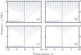
Figure 6: Spectrum of MP waves supported by a 2D electron gas confined at the surface of a sphere with radius $100\;\mu\hbox{m}$. The magnetic field includes superimposed spherically symmetric component $B_{\mathrm{C}}$ which is equal to $0.4B_{0}$ (a), $0.8B_{0}$ (b), $1.2B_{0}$ (c) and $1.6B_{0}$ (d). Here $B_{0}$ is magnitude of uniform magnetic field. For $B_{\mathrm{C}}>B_{0}$, Kelvin and Yanai modes disappear as expected, but the Rossby modes are still present.

B.4 B4. Rossby MP waves in the presence of superimposed spherically symmetric magnetic field

The mathematical origin of Kelvin and Yanai modes is intricately related with the topology of the bulk MP waves spectrum. As a result, their presence requires magnetic field to switch its sign across the equator. However, it is not the case for the Rossby waves. This can be demonstrated if we superimpose spherically symmetric and uniform magnetic fields. The corresponding radial component $B_{\mathbf{r}}^{\mathrm{R}}=B_{0}\cos(\theta)+B_{\mathrm{C}}$ is latitude dependent, but does not involve the sign change if $B_{\mathrm{C}}>B_{0}$. The spectrum of MP waves is presented in Fig. (6) for sphere radius $100\;\mu\hbox{m}$ (all other parameters are the same as in the main part of the paper) and superimposed magnetic field given by $0.4B_{0}$ (a), $0.8B_{0}$ (b), $1.2B_{0}$ (c) and $1.6B_{0}$ (d). As long as $B_{\mathrm{C}}<B_{0}$, the presence of Kelvin and Yanai modes are clearly visible, and their spectrum is weakly modified compared to $B_{\mathrm{C}}=0$. For $B_{\mathrm{C}}>B_{0}$, Kelvin and Yanai modes disappear as expected, but the topologically trivial Rossby modes are still present.

References

- Burkov (2018) A. Burkov, Weyl Metals, Annual Review of Condensed Matter Physics 9, 359 (2018).
- Hasan and Kane (2010) M. Z. Hasan and C. L. Kane, Colloquium: Topological insulators, Rev. Mod. Phys. 82, 3045 (2010).
- Sato and Ando (2017) M. Sato and Y. Ando, Topological superconductors: a review, Reports on Progress in Physics 80, 076501 (2017).
- Lu et al. (2014) L. Lu, J. D. Joannopoulos, and M. Soljačić, Topological photonics, Nature Photonics 8, 821 (2014).
- Ozawa et al. (2019) T. Ozawa, H. M. Price, A. Amo, N. Goldman, M. Hafezi, L. Lu, M. C. Rechtsman, D. Schuster, J. Simon, O. Zilberberg, and I. Carusotto, Topological photonics, Rev. Mod. Phys. 91, 015006 (2019).
- Kim et al. (2020) M. Kim, Z. Jacob, and J. Rho, Recent advances in 2D, 3D and higher-order topological photonics, Light: Science & Applications 9, 130 (2020).
- Lee et al. (2018) C. H. Lee, S. Imhof, C. Berger, F. Bayer, J. Brehm, L. W. Molenkamp, T. Kiessling, and R. Thomale, Topolectrical Circuits, Communications Physics 1, 39 (2018).
- Dong et al. (2021) J. Dong, V. Juričić, and B. Roy, Topolectric circuits: Theory and construction, Phys. Rev. Research 3, 023056 (2021).
- Bergholtz et al. (2021) E. J. Bergholtz, J. C. Budich, and F. K. Kunst, Exceptional topology of non-Hermitian systems, Rev. Mod. Phys. 93, 015005 (2021).
- Kawabata et al. (2019) K. Kawabata, K. Shiozaki, M. Ueda, and M. Sato, Symmetry and Topology in Non-Hermitian Physics, Phys. Rev. X 9, 041015 (2019).
- Yoshida and Hatsugai (2019) T. Yoshida and Y. Hatsugai, Exceptional rings protected by emergent symmetry for mechanical systems, Phys. Rev. B 100, 054109 (2019).
- Matsuno (1966) T. Matsuno, Quasi-Geostrophic Motions in the Equatorial Area, Journal of the Meteorological Society of Japan. Ser. II 44, 25 (1966).
- Vallis (2006) G. K. Vallis, Atmospheric and Oceanic Fluid Dynamics (Cambridge University Press, Cambridge, U.K., 2006) p. 745.
- Delplace et al. (2017) P. Delplace, J. B. Marston, and A. Venaille, Topological origin of equatorial waves, Science 358, 1075 (2017).
- Dyakonov and Shur (1993) M. Dyakonov and M. Shur, Shallow water analogy for a ballistic field effect transistor: New mechanism of plasma wave generation by dc current, Phys. Rev. Lett. 71, 2465 (1993).
- Chaplik (1972) A. V. Chaplik, Possible Crystallization of Charge Carriers in Low-density Inversion Layers, Journal of Experimental and Theoretical Physics 35, 395 (1972).
- Note (1) Plasma waves in the presence of a magnetic field are usually referred to as magnetoplasma waves or magnetoplasmons.
- Jin et al. (2016) D. Jin, L. Lu, Z. Wang, C. Fang, J. D. Joannopoulos, M. Soljačić, L. Fu, and N. X. Fang, Topological magnetoplasmon, Nature Communications 7, 13486 (2016).
- Fetter (1985) A. L. Fetter, Edge magnetoplasmons in a bounded two-dimensional electron fluid, Phys. Rev. B 32, 7676 (1985).
- Note (2) For electrons with conventional quadratic dispersion, this term is equal to their band mass. For electrons with unconventional but isotropic dispersion (e.g., with relativistic-like Dirac dispersion), the mass is given by the ratio between the Fermi energy and Fermi velocity .
-
Note (3)
The explicit expression for is given by
where is the complex conjugation operator. - Ryu et al. (2010) S. Ryu, A. P. Schnyder, A. Furusaki, and A. W. W. Ludwig, Topological insulators and superconductors: tenfold way and dimensional hierarchy, New Journal of Physics 12, 065010 (2010).
-
Note (4)
Explicit expressions for the components of spin-1 Pauli
matrices are given by
. - Note (5) The motion of the electrons is confined to the plane, but interactions are mediated by an electric field that is extended in three-dimensional space.
- Tauber et al. (2020) C. Tauber, P. Delplace, and A. Venaille, Anomalous bulk-edge correspondence in continuous media, Phys. Rev. Research 2, 013147 (2020).
- Graf et al. (2021) G. M. Graf, H. Jud, and C. Tauber, Topology in Shallow-Water Waves: A Violation of Bulk-Edge Correspondence, Communications in Mathematical Physics 383, 731 (2021).
- Tauber and Thiang (2021) C. Tauber and G. C. Thiang, Topology in shallow-water waves: A spectral flow perspective (2021), arXiv:2110.04097 [math-ph] .
- Faure (2019) F. Faure, Manifestation of the topological index formula in quantum waves and geophysical waves (2019), arXiv:1901.10592 [math-ph] .
- Tauber et al. (2019) C. Tauber, P. Delplace, and A. Venaille, A bulk-interface correspondence for equatorial waves, Journal of Fluid Mechanics 868, R2 (2019).
- Fu and Qin (2021) Y. Fu and H. Qin, Topological phases and bulk-edge correspondence of magnetized cold plasmas, Nature Communications 12, 3924 (2021).
- Note (6) The kink profile implies that and . It should also be noted that the mathematical structure of this solution is reminiscent of the celebrated Jackiw-Rebbi solution for the massive Dirac model with position-dependent mass Jackiw and Rebbi (1976).
- Cooper et al. (1995) F. Cooper, A. Khare, and U. Sukhatme, Supersymmetry and quantum mechanics, Physics Reports 251, 267 (1995).
- Çevik et al. (2016) D. Çevik, M. Gadella, Ş. Kuru, and J. Negro, Resonances and antibound states for the Pöschl–Teller potential: Ladder operators and SUSY partners, Physics Letters A 380, 1600 (2016).
- Note (7) At , the prefactor is positive, which ensures the presence of at least one bound state trapped by the PT quantum well potential.
- Note (8) We use for the integer part of a real number.
- Note (9) In the presence of the domain wall, the inversion symmetry is broken, and these modes are no longer pinned at zero frequency.
- Zaqarashvili et al. (2021) T. V. Zaqarashvili, M. Albekioni, J. L. Ballester, Y. Bekki, L. Biancofiore, A. C. Birch, M. Dikpati, L. Gizon, E. Gurgenashvili, E. Heifetz, A. F. Lanza, S. W. McIntosh, L. Ofman, R. Oliver, B. Proxauf, O. M. Umurhan, and R. Yellin-Bergovoy, Rossby Waves in Astrophysics, Space Science Reviews 217, 15 (2021).
- Note (10) We ignore the disorder-induced residual metallic bulk conductivity that usually appears in topological insulators, including samples. For thin films with thickness , the response has been argued to be fully dominated by the Dirac states.
- Campos et al. (2018) W. H. Campos, J. M. Fonseca, V. E. de Carvalho, J. B. S. Mendes, M. S. Rocha, and W. A. Moura-Melo, Topological Insulator Particles As Optically Induced Oscillators: Toward Dynamical Force Measurements and Optical Rheology, ACS Photonics 5, 741 (2018).
- Hamdou et al. (2013) B. Hamdou, J. Gooth, A. Dorn, E. Pippel, and K. Nielsch, Surface state dominated transport in topological insulator Bi2Te3 nanowires, Applied Physics Letters 103, 193107 (2013), https://doi.org/10.1063/1.4829748 .
- Cho et al. (2015) S. Cho, B. Dellabetta, R. Zhong, J. Schneeloch, T. Liu, G. Gu, M. J. Gilbert, and N. Mason, Aharonov–Bohm oscillations in a quasi-ballistic three-dimensional topological insulator nanowire, Nature Communications 6, 7634 (2015).
- Münning et al. (2021) F. Münning, O. Breunig, H. F. Legg, S. Roitsch, D. Fan, M. Rößler, A. Rosch, and Y. Ando, Quantum confinement of the Dirac surface states in topological-insulator nanowires, Nature Communications 12, 1038 (2021).
- Kunakova et al. (2018) G. Kunakova, L. Galletti, S. Charpentier, J. Andzane, D. Erts, F. Léonard, C. D. Spataru, T. Bauch, and F. Lombardi, Bulk-free topological insulator Bi2Se3 nanoribbons with magnetotransport signatures of Dirac surface states, Nanoscale 10, 19595 (2018).
- Ziegler et al. (2018) J. Ziegler, R. Kozlovsky, C. Gorini, M.-H. Liu, S. Weishäupl, H. Maier, R. Fischer, D. A. Kozlov, Z. D. Kvon, N. Mikhailov, S. A. Dvoretsky, K. Richter, and D. Weiss, Probing spin helical surface states in topological HgTe nanowires, Phys. Rev. B 97, 035157 (2018).
- Jauregui et al. (2015) L. A. Jauregui, M. T. Pettes, L. P. Rokhinson, L. Shi, and Y. P. Chen, Gate Tunable Relativistic Mass and Berry’s phase in Topological Insulator Nanoribbon Field Effect Devices, Scientific Reports 5, 8452 (2015).
- Dufouleur et al. (2017) J. Dufouleur, L. Veyrat, B. Dassonneville, E. Xypakis, J. H. Bardarson, C. Nowka, S. Hampel, J. Schumann, B. Eichler, O. G. Schmidt, B. Büchner, and R. Giraud, Weakly-coupled quasi-1D helical modes in disordered 3D topological insulator quantum wires, Scientific Reports 7, 45276 (2017).
- Autore et al. (2015) M. Autore, H. Engelkamp, F. D’Apuzzo, A. D. Gaspare, P. D. Pietro, I. L. Vecchio, M. Brahlek, N. Koirala, S. Oh, and S. Lupi, Observation of Magnetoplasmons in Bi2Se3 Topological Insulator, ACS Photonics 2, 1231 (2015).
- Note (11) In this regime, MP waves hybridize with light and become polaritons.
- Bernstein (1958) I. B. Bernstein, Waves in a Plasma in a Magnetic Field, Phys. Rev. 109, 10 (1958).
- Chiu and Quinn (1974) K. W. Chiu and J. J. Quinn, Plasma oscillations of a two-dimensional electron gas in a strong magnetic field, Phys. Rev. B 9, 4724 (1974).
- Volkov and Zabolotnykh (2014) V. A. Volkov and A. A. Zabolotnykh, Bernstein modes and giant microwave response of a two-dimensional electron system, Phys. Rev. B 89, 121410 (2014).
- Roldán et al. (2011) R. Roldán, M. O. Goerbig, and J.-N. Fuchs, Theory of Bernstein modes in graphene, Phys. Rev. B 83, 205406 (2011).
- Batke et al. (1985) E. Batke, D. Heitmann, J. P. Kotthaus, and K. Ploog, Nonlocality in the Two-Dimensional Plasmon Dispersion, Phys. Rev. Lett. 54, 2367 (1985).
- Batke et al. (1986) E. Batke, D. Heitmann, and C. W. Tu, Plasmon and magnetoplasmon excitation in two-dimensional electron space-charge layers on GaAs, Phys. Rev. B 34, 6951 (1986).
- Holland et al. (2004) S. Holland, C. Heyn, D. Heitmann, E. Batke, R. Hey, K. J. Friedland, and C.-M. Hu, Quantized Dispersion of Two-Dimensional Magnetoplasmons Detected by Photoconductivity Spectroscopy, Phys. Rev. Lett. 93, 186804 (2004).
- Richards (2000) D. Richards, Inelastic light scattering from inter-Landau level excitations in a two-dimensional electron gas, Phys. Rev. B 61, 7517 (2000).
- Bandurin et al. (2022) D. A. Bandurin, E. Mönch, K. Kapralov, I. Y. Phinney, K. Lindner, S. Liu, J. H. Edgar, I. A. Dmitriev, P. Jarillo-Herrero, D. Svintsov, and S. D. Ganichev, Cyclotron resonance overtones and near-field magnetoabsorption via terahertz Bernstein modes in graphene, Nature Physics 18, 462 (2022).
- Allen et al. (1983) S. J. Allen, H. L. Störmer, and J. C. M. Hwang, Dimensional resonance of the two-dimensional electron gas in selectively doped GaAs/AlGaAs heterostructures, Phys. Rev. B 28, 4875 (1983).
- Kumada et al. (2014) N. Kumada, P. Roulleau, B. Roche, M. Hashisaka, H. Hibino, I. Petković, and D. C. Glattli, Resonant Edge Magnetoplasmons and Their Decay in Graphene, Phys. Rev. Lett. 113, 266601 (2014).
- Crassee et al. (2012) I. Crassee, M. Orlita, M. Potemski, A. L. Walter, M. Ostler, T. Seyller, I. Gaponenko, J. Chen, and A. B. Kuzmenko, Intrinsic Terahertz Plasmons and Magnetoplasmons in Large Scale Monolayer Graphene, Nano Letters 12, 2470 (2012).
- Yan et al. (2012) H. Yan, Z. Li, X. Li, W. Zhu, P. Avouris, and F. Xia, Infrared Spectroscopy of Tunable Dirac Terahertz Magneto-Plasmons in Graphene, Nano Letters 12, 3766 (2012).
- Jin et al. (2019) D. Jin, Y. Xia, T. Christensen, M. Freeman, S. Wang, K. Y. Fong, G. C. Gardner, S. Fallahi, Q. Hu, Y. Wang, L. Engel, Z.-L. Xiao, M. J. Manfra, N. X. Fang, and X. Zhang, Topological kink plasmons on magnetic-domain boundaries, Nature Communications 10, 4565 (2019).
- Tan et al. (2008) P. S. Tan, X.-C. Yuan, J. Lin, Q. Wang, T. Mei, R. E. Burge, and G. G. Mu, Surface plasmon polaritons generated by optical vortex beams, Applied Physics Letters 92, 111108 (2008).
- Sakai et al. (2015) K. Sakai, K. Nomura, T. Yamamoto, and K. Sasaki, Excitation of Multipole Plasmons by Optical Vortex Beams, Scientific Reports 5, 8431 (2015).
- Ge et al. (2015) L. Ge, D. Han, and J. Zi, Electromagnetic scattering by spheres of topological insulators, Optics Communications 354, 225 (2015).
- Lakhtakia and Mackay (2016) A. Lakhtakia and T. G. Mackay, Electromagnetic scattering by homogeneous, isotropic, dielectric–magnetic sphere with topologically insulating surface states, J. Opt. Soc. Am. B 33, 603 (2016).
- Schultz et al. (2020) J. Schultz, F. S. Nogueira, B. Büchner, J. v. d. Brink, and A. Lubk, Axion Mie Theory of Electron Energy Loss Spectroscopy in Topological Insulators (2020).
- Imura et al. (2011) K.-I. Imura, Y. Takane, and A. Tanaka, Spin Berry phase in anisotropic topological insulators, Phys. Rev. B 84, 195406 (2011).
- Governale et al. (2020) M. Governale, B. Bhandari, F. Taddei, K.-I. Imura, and U. Zülicke, Finite-size effects in cylindrical topological insulators, New Journal of Physics 22, 063042 (2020).
- Imura et al. (2012) K.-I. Imura, Y. Yoshimura, Y. Takane, and T. Fukui, Spherical topological insulator, Phys. Rev. B 86, 235119 (2012).
- Gioia et al. (2019) L. Gioia, M. G. Christie, U. Zülicke, M. Governale, and A. J. Sneyd, Spherical topological insulator nanoparticles: Quantum size effects and optical transitions, Phys. Rev. B 100, 205417 (2019).
- Siroki et al. (2016) G. Siroki, D. K. K. Lee, P. D. Haynes, and V. Giannini, Single-electron induced surface plasmons on a topological nanoparticle, Nature Communications 7, 12375 (2016).
- Raghu et al. (2010) S. Raghu, S. B. Chung, X.-L. Qi, and S.-C. Zhang, Collective Modes of a Helical Liquid, Phys. Rev. Lett. 104, 116401 (2010).
- Efimkin et al. (2012a) D. K. Efimkin, Y. E. Lozovik, and A. A. Sokolik, Collective excitations on a surface of topological insulator, Nanoscale Research Letters 7, 163 (2012a).
- Efimkin et al. (2012b) D. Efimkin, Y. Lozovik, and A. Sokolik, Spin-plasmons in topological insulator, Journal of Magnetism and Magnetic Materials 324, 3610 (2012b).
- Stauber et al. (2013) T. Stauber, G. Gómez-Santos, and L. Brey, Spin-charge separation of plasmonic excitations in thin topological insulators, Phys. Rev. B 88, 205427 (2013).
- Efimkin and Kargarian (2021) D. K. Efimkin and M. Kargarian, Topological spin-plasma waves, Phys. Rev. B 104, 075413 (2021).
- Lai et al. (2014) Y.-P. Lai, I.-T. Lin, K.-H. Wu, and J.-M. Liu, Plasmonics in Topological Insulators, Nanomaterials and Nanotechnology 4, 13 (2014).
- Averitt et al. (1997) R. D. Averitt, D. Sarkar, and N. J. Halas, Plasmon Resonance Shifts of Au-Coated Nanoshells: Insight into Multicomponent Nanoparticle Growth, Phys. Rev. Lett. 78, 4217 (1997).
- Daneshfar and Bazyari (2014) N. Daneshfar and K. Bazyari, Optical and spectral tunability of multilayer spherical and cylindrical nanoshells, Applied Physics A 116, 611 (2014).
- Perera et al. (2020) T. Perera, S. D. Gunapala, M. I. Stockman, and M. Premaratne, Plasmonic Properties of Metallic Nanoshells in the Quantum Limit: From Single Particle Excitations to Plasmons, The Journal of Physical Chemistry C 124, 27694 (2020).
- Mikhailov and Volkov (1992) S. A. Mikhailov and V. A. Volkov, Inter-edge magnetoplasmons in inhomogeneous two-dimensional electron systems, Journal of Physics: Condensed Matter 4, 6523 (1992).
- Aleiner and Glazman (1994) I. L. Aleiner and L. I. Glazman, Novel edge excitations of two-dimensional electron liquid in a magnetic field, Phys. Rev. Lett. 72, 2935 (1994).
- Xia and Quinn (1994) X. Xia and J. J. Quinn, Edge magnetoplasmons of two-dimensional electron-gas systems, Phys. Rev. B 50, 11187 (1994).
- Song and Rudner (2016) J. C. W. Song and M. S. Rudner, Chiral plasmons without magnetic field, Proceedings of the National Academy of Sciences 113, 4658 (2016), https://www.pnas.org/doi/pdf/10.1073/pnas.1519086113 .
- Petrov (2021) A. S. Petrov, Plasmonic excitation for a tunable transmitter without magnetic field immune to backscattering, Phys. Rev. B 104, L241407 (2021).
- Sokolik et al. (2021) A. A. Sokolik, O. V. Kotov, and Y. E. Lozovik, Plasmonic modes at inclined edges of anisotropic two-dimensional materials, Phys. Rev. B 103, 155402 (2021).
- Jackiw and Rebbi (1976) R. Jackiw and C. Rebbi, Solitons with fermion number ½, Phys. Rev. D 13, 3398 (1976).