Effective spin models of Kerr-nonlinear parametric oscillators for quantum annealing

Abstract

A method of quantum annealing (QA) using Kerr-nonlinear parametric oscillators (KPOs) was proposed. This method is described by bosonic operators and has different characteristics from QA based on the transverse-field Ising model. As the first step to describe this method in the conventional framework of QA, we propose effective spin models of KPOs. The spin models are obtained via a variant of the Holstein-Primakoff transformation and are described by spin-$s$ operators. The terms for detuning, coherent driving, parametric driving, and the Kerr effect are mapped to the transverse field, longitudinal field, nonlinear terms for the z- and x-components of spins, respectively. By analyzing the spin models corresponding to KPOs in several settings, we demonstrate that the present spin models for a rather large $s$ and tuned parameters qualitatively reproduce behavior of KPOs.

I Introduction

Quantum annealing (QA) is a heuristic to solve combinatorial optimization problems by embedding the problems in systems with quantum fluctuations [1, 2, 3, 4]. In the ideal scenario for QA, the system follows the instantaneous ground state during the gradual decrease of quantum fluctuations and finally reaches the ground state that corresponds to the solution of the problem. It is natural to utilize the Ising model, which represents the problems [5], with simple extra terms for quantum fluctuations. The transverse-field Ising model (TFIM) is such a model and has been typically used in studies of QA [2, 3, 4]. Such studies have been also inspired by the advent of quantum annealers provided by D-Wave Systems Inc. [6], which are well described by the TFIM. Variants of the model including other terms for quantum fluctuations, e.g., non-stoquastic catalysts [7, 8, 9, 10, 11, 12, 13, 14, 15], have been also investigated. Thus QA has been studied primarily in terms of the TFIM and its variants.

QA, however, does not have to be described by spin systems. Indeed, a method related to QA was proposed using Kerr-nonlinear parametric osicllators (KPOs) [16, 17]. KPOs are represented by bosonic operators and have continuous degrees of freedom, but final states can be associated with the Ising model [16, 17]. The pump amplitude for the parametric driving is gradually increased in this method. This adiabatic process for a KPO generates the cat state, i.e., superposition of two coherent states with opposite phases [16, 17, 18] in which we can encode the up and down states of an Ising spin. The underlying mechanism to obtain Ising spins is interpreted as bifurcation [16, 17]. The ground state of the Ising model can be obtained by applying this method to networks of interacting KPOs. We consider this method in terms of a kind of QA and simply call it QA with KPOs hereafter.

QA with KPOs has been intensively studied [16, 17, 19, 20, 21, 22, 23, 24, 25, 26, 27, 28]. The efficiency of this method was demonstrated with simulations of small systems [16, 17, 19]. Subsequent studies pointed out the possibility of applications to the Lechner-Hauke-Zoller scheme [29] with four- or three-body interactions [19, 20, 21], Boltzmann sampling [22], and QA using excited states [23, 24]. The bifurcation-based approach to QA has also been studied using a spin model [30]. A KPO is not just a theoretical model and is realized in superconducting circuits with the Josephson junctions [31, 32, 33]. The physical implementation of QA with KPOs is also expected [25, 19, 21, 28]. Qubits generated by the adiabatic process for KPOs can be utilized for the gate-based quantum computation [34, 18, 32, 35, 36, 37, 38, 39].

One of the characteristics of QA with KPOs is being described by bosonic operators. This point highlights a difference from conventional QA based on the TFIM but also makes it difficult to understand this method with the concepts developed in the study of the conventional QA. It is a natural question how this method can be described in terms of the conventional QA. The first step to answer this question is to construct effective spin models for KPOs. The models should be as simple as the TFIM. Such spin models enable us to discuss the two methods at the same stage, where the systems are represented by spins. The spin representation would more clearly show the role of each parameter of KPOs in QA. In this regard, identifying the correspondence to spin models is similar in purpose to the gate synthesis problem discussed in gate-based quantum computation [40, 41]. Note that a spin model was proposed for the bifurcation-based QA as mentioned above [30], but this model was not derived from KPOs. An effective spin model for KPOs could clarify the relation between the previously proposed spin model and KPOs.

In this paper, we propose effective spin models for KPOs. We aim to find simple spin models that qualitatively reproduce behavior of KPOs and clarify roles of parameters of KPOs in QA. The next section gives a brief review of QA with KPOs. In Sec. III, the spin models are derived via the Holstein-Primakoff (HP) transformation [42, 43]. In Sec. IV, we compare physical quantities such as photon number computed for the bosonic models of KPOs and their spin counterparts computed for the corresponding spin models. We present conclusion in Sec. V

II Quantum annealing with Kerr-nonlinear parametric oscillators

KPOs are typically investigated in the frame rotating at half the frequency of the parametric driving. A KPO in the frame under the rotating-wave approximation is governed by [16, 17]

$$\hat{H}_{\text{b}}=\Delta\hat{a}^{\dagger}\hat{a}+\frac{K}{2}\hat{a}^{\dagger 2}\hat{a}^{2}-\frac{p}{2}(\hat{a}^{\dagger 2}+\hat{a}^{2})-\epsilon(\hat{a}^{\dagger}+\hat{a}),$$ (1)

where $\hat{a}^{\dagger}$ and $\hat{a}$ are bosonic creation and annihilation operators, respectively. The subscript b emphasizes that this is a Hamiltonian for bosons. This is a model, for example, of superconducting circuits with the Josephson junctions [31, 32, 33]. The parametric driving with the pump amplitude $p$ is controlled by the modulated magnetic flux through SQUIDs. The Kerr nonlinearlity $K$ stems from the nonlinearlity of the Josephson junctions. The detuning $\Delta$ represents the difference of the oscillator frequency from half the pump frequency. The coherent driving is applied with amplitude $\epsilon$ to generate the bias in the system. However, the investigation in this paper is not restricted to specific implementations to superconducting circuits. Note that $\hbar=1$ throughout the paper.

QA with KPOs is carried out by varying the pump amplitude [16]. We prepare the ground state of the system for $p=0$ and $\Delta>0$ and gradually increase $p$. If the energy gap between the ground state and excited states does not close in the annealing passage, the system will track the instantaneous ground state for temporal $p$ [3]. Consequently, we will obtain the ground state of the KPO for large $p$. Let us assume $\epsilon=0$ for simplicity. The initial state is the vacuum state. For large $p$, where $\Delta$ can be ignored, the Hamiltonian is written as

$$\hat{H}_{\text{b}}=\frac{K}{2}\left(\hat{a}^{\dagger 2}-\alpha_{0}^{2}\right)\left(\hat{a}^{2}-\alpha_{0}^{2}\right),$$ (2)

where $\alpha_{0}=\sqrt{p/K}$. The ground state obtained by QA starting from the vacuum state is the so-called even cat state, $(|\alpha_{0}\rangle+|-\alpha_{0}\rangle)/\sqrt{2}$, where a coherent state $|\alpha\rangle$ is defined as $\hat{a}|\alpha\rangle=\alpha|\alpha\rangle$ [44]. Both $|\alpha_{0}\rangle$ and $|-\alpha_{0}\rangle$ are eigenstates of the Hamiltonian with the same eigenvalue. The final state is their superposition and has the same parity as the initial state, namely the even parity, since the Hamiltonian commutes the parity operator that leads to $\hat{a}\to-\hat{a}$. If we also gradually increase the coherent driving, the ground state for large $p$ is not the cat state but a state localized in one of the double wells in the meta-potential for the KPO. If the absolute value of $\epsilon$ is small compared to $p$, the state is close to $|\alpha_{0}\rangle$ for $\epsilon>0$ and $|-\alpha_{0}\rangle$ for $\epsilon<0$ [19]. This relation is reminescent of an Ising spin in a magnetic field [45]. In addition, $|\alpha_{0}\rangle$ and $|-\alpha_{0}\rangle$ for large $\alpha_{0}$ are approximately orthogonal, since $\langle\alpha_{0}|-\alpha_{0}\rangle=e^{-2\alpha_{0}^{2}}$ [44]. Therefore, we can encode an Ising spin $\{\uparrow,\downarrow\}$ in the states $\{|\alpha_{0}\rangle,|-\alpha_{0}\rangle\}$ and interpret the coherent driving as the magnetic field applied to the spin.

The Ising model is artificially realized by networks of interacting KPOs [16],

$$\hat{H}_{\text{b}}^{(N)}=\sum_{i=1}^{N}\hat{H}_{\text{b},i}-\xi_{0}\sum_{i,j}J_{ij}\hat{a}^{\dagger}_{i}\hat{a}_{j},$$ (3)

$$\hat{H}_{\text{b},i}=\Delta\hat{a}^{\dagger}_{i}\hat{a}_{i}+\frac{K}{2}\hat{a}^{\dagger 2}_{i}\hat{a}^{2}_{i}-\frac{p}{2}(\hat{a}^{\dagger 2}_{i}+\hat{a}^{2}_{i})-\epsilon_{i}(\hat{a}^{\dagger}_{i}+\hat{a}_{i}),$$ (4)

where $J_{ij}$ will correspond to the coupling constant of Ising spins $i$ and $j$. The parameter $\xi_{0}$ is introduced to satisfy that the vacuum state is the ground state of the initial Hamiltonian for $p=0$ and $\epsilon=0$ [16, 17]. For sufficiently large $p$, where $\Delta$ is ignored, each KPO in the ground state is approximately described by one of the two coherent states $|\sigma\alpha_{0}\rangle$ with $\sigma=\pm 1$ representating an Ising spin. Hence, the ground state of the whole system can be expressed as $|\bm{\sigma}\rangle=|\sigma_{1}\alpha_{0}\rangle\cdots|\sigma_{N}\alpha_{0}\rangle$. The expectation value of the energy for $|\bm{\sigma}\rangle$ is

$$\langle\bm{\sigma}|\hat{H}_{\text{b}}^{(N)}|\bm{\sigma}\rangle=-2\alpha_{0}\sum_{i=1}^{N}\epsilon_{i}\sigma_{i}-\xi_{0}\alpha_{0}^{2}\sum_{i,j}J_{ij}\sigma_{i}\sigma_{j},$$ (5)

where constants are dropped. This relation maps the ground state of the KPOs to that of the Ising model. We can obtain the ground state of the KPOs with the gradual increase of $p$. Thus, the ground state of the Ising model is found with this scheme. This mapping to Ising spins requires the ground state to be composed of the coherent states with the same amplitude. This is guaranteed for large $p$, but the system for not large $p$ is not necessarily in such a state. We need to assume more complicated states to describe the system in the intermediate range of $p$.

III Transformation

We utilize the Holstein-Primakoff (HP) transformation [42, 43] to obtain spin models for KPOs. The HP transformation is defined by

$$\hat{S}^{+} =\sqrt{2S-\hat{a}^{\dagger}\hat{a}}\hat{a},$$ (6)

$$\hat{S}^{-} =\hat{a}^{\dagger}\sqrt{2S-\hat{a}^{\dagger}\hat{a}},$$ (7)

$$\hat{S}^{z} =S-\hat{a}^{\dagger}\hat{a},$$ (8)

where $\hat{S}^{\pm}=\hat{S}^{x}\pm i\hat{S}^{y}$, and $\hat{S}^{x}$, $\hat{S}^{y}$, and $\hat{S}^{z}$ are the x-, y-, and z-components of the spin-$S$ operator. $S$ is an integer or half-integer. The spin operators obey $[\hat{S}^{\alpha},\hat{S}^{\beta}]=i\epsilon^{\alpha\beta\gamma}\hat{S}^{\gamma}$, where $\alpha$, $\beta$, $\gamma$ run over $x$, $y$, $z$, and $\epsilon^{\alpha\beta\gamma}$ is the totally antisymmetric tensor. $[\hat{a},\hat{a}^{\dagger}]=1$ also holds. We can map spin systems to bosonic ones with the above relation, but the Fock states for the bosonic ones with photon number larger than $2S$ are unphysical states for the original spin systems. Therefore, we only consider the subspace spanned by the Fock states with photon number equal to or smaller than $2S$, while the other states are eliminated by a projector. In typical treatment [42, 43], the square root for $S^{+}$ or $S^{-}$ is expanded in powers of $1/S$,

$$\hat{S}^{+}=\sqrt{2S}\left[1-\frac{\hat{a}^{\dagger}\hat{a}}{4S}-\frac{(\hat{a}^{\dagger}\hat{a})^{2}}{32S^{2}}-\cdots\right]\hat{a}.$$ (9)

This can be interpreted as the expansion in powers of $\hat{a}^{\dagger}\hat{a}/2S$. Other similar approaches [46] such as the Schwinger bosons and the Dyson-Maleev transformation can be applied, but the former requires multiple boson species to represent a spin, and the latter breaks Hermeticity. We therefore adopt the HP transformation. Note that a more sophisticated version of the HP transformation has recently been proposed [47, 48], but we concentrate in this paper on examining the approach based on the original one.

We use the HP transformation in the opposite direction to transform KPOs to spin models. In addition, we apply the gauge transformation, $(\hat{S}^{x},\hat{S}^{y},\hat{S}^{z})\to(\hat{s}^{z},-\hat{s}^{y},\hat{s}^{x})$, which preserves the spin commutation relation. Here, spin operators for the latter gauge are represented with lowercase letters to distinguish the gauges. For example, the vacuum state, which is the initial state in QA with KPOs, is mapped to the eigenstate $|m=s,s\rangle_{x}$ of $\hat{s}^{x}$ for eigenvalue $s$. We also slightly modify the expansion and expand the square root in powers of $\hat{a}^{\dagger}\hat{a}/2s$ at $\alpha^{2}/2s$, where $\alpha^{2}$ will be set to some value. Then $\hat{S}^{+}$ in Eq. (9) is rewritten as

$$\hat{s}^{-}= \hat{s}^{z}-i\hat{s}^{y}$$

$$= \sqrt{2s-\hat{a}^{\dagger}\hat{a}}\hat{a}$$

$$= \sqrt{2s}\Bigg{[}\sqrt{1-\frac{\alpha^{2}}{2s}}-\frac{\hat{a}^{\dagger}\hat{a}-\alpha^{2}}{4s\sqrt{1-\frac{\alpha^{2}}{2s}}}$$ (10)

$$-\frac{(\hat{a}^{\dagger}\hat{a}-\alpha^{2})^{2}}{32s^{2}\left(1-\frac{\alpha^{2}}{2s}\right)^{3/2}}-\cdots\Bigg{]}\hat{a}.$$

We also have

$$\hat{s}^{x} =s-\hat{a}^{\dagger}\hat{a},$$ (11)

$$\hat{s}^{y} =\frac{\sqrt{2s}}{i}\Bigg{[}\sqrt{1-\frac{\alpha^{2}}{2s}}\frac{\hat{a}^{\dagger}-\hat{a}}{2}$$ (12)

$$-\frac{\hat{a}^{\dagger 2}\hat{a}-\hat{a}^{\dagger}\hat{a}^{2}-\alpha^{2}(\hat{a}^{\dagger}-\hat{a})}{8s\sqrt{1-\frac{\alpha^{2}}{2s}}}+\cdots\Bigg{]}.$$

$$\hat{s}^{z} =\sqrt{2s}\Bigg{[}\sqrt{1-\frac{\alpha^{2}}{2s}}\frac{\hat{a}^{\dagger}+\hat{a}}{2}$$ (13)

$$-\frac{\hat{a}^{\dagger 2}\hat{a}+\hat{a}^{\dagger}\hat{a}^{2}-\alpha^{2}(\hat{a}^{\dagger}+\hat{a})}{8s\sqrt{1-\frac{\alpha^{2}}{2s}}}+\cdots\Bigg{]}.$$

We use this relation to represent the terms in $\hat{H}_{\text{b}}$ [Eq. (1)] with $\hat{s}^{x}$ and $\hat{s}^{z}$ as follows:

$$\hat{a}^{\dagger}\hat{a} =s-\hat{s}^{x},$$ (14)

$$\hat{a}^{\dagger 2}\hat{a}^{2} =(\hat{s}^{x})^{2}-(2s-1)\hat{s}^{x}+s(s-1),$$ (15)

$$\frac{\hat{a}^{\dagger}+\hat{a}}{2} =\frac{1}{\sqrt{2s-\alpha^{2}}}\hat{s}^{z}+\cdots,$$ (16)

$$\frac{\hat{a}^{\dagger 2}+\hat{a}^{2}}{2} =-s+\hat{s}^{x}-\frac{1}{2}+\frac{2}{2s-\alpha^{2}}(\hat{s}^{z})^{2}+\cdots.$$ (17)

Here, the value of $s$ is not specified, but $\alpha^{2}<2s$ is assumed. The leading terms shown in Eqs. (16) and (17) are obtained from Eq. (11) and the first term in Eq. (13). Their higher order terms obtained from the second term in Eq. (13) are shown in Appendix.

According to Eqs. (11)–(17), $\hat{H}_{\text{b}}$ is transformed to

$$\hat{H}_{\text{s}}= -\frac{2p}{2s-\alpha^{2}}(\hat{s}^{z})^{2}-\left[\Delta+p+\left(s-\frac{1}{2}\right)K\right]\hat{s}^{x}$$ (18)

$$+\frac{K}{2}(\hat{s}^{x})^{2}-\frac{2\epsilon}{\sqrt{2s-\alpha^{2}}}\hat{s}^{z},$$

where higher order terms and constants are dropped. The subscript s emphasizes that this is a Hamiltonian for spins. Detuning $\Delta$ works as a transverse field, while the coherent driving $\epsilon$ turns to a longitudinal field. The Kerr term generates the nonlinearlity of $\hat{s}^{x}$. Larger pump amplitude $p$ enhances fluctuations associated with $\hat{s}^{z}$, which is what we mainly control in QA with KPOs and causes the bifurcation. Since the nonlinear terms cannot be represented with spin-1/2 operators, $\hat{H}_{\text{s}}$ needs $s\geq 1$ to describe QA with the bifurcation mechanism. $\hat{H}_{\text{s}}$ for $s=1$ without $(\hat{s}^{x})^{2}$ has the same form as a model for bifurcation-based QA [30]. Thus $\hat{H}_{\text{s}}$ bridges a gap between KPOs and bifurcation-based QA with spin models by clarifying coefficients of the spin operators as a function of the parameters of KPOs.

The Hamiltonian of interacting KPOs [Eq. (3)] is tranformed to

$$\hat{H}_{\text{s}}^{(N)}=\sum_{i=1}^{N}\hat{H}_{\text{s},i}-\frac{2\xi_{0}}{2s-\alpha^{2}}\sum_{i<j}J_{ij}\left(\hat{s}^{z}_{i}\hat{s}^{z}_{j}+\hat{s}^{y}_{i}\hat{s}^{y}_{j}\right),$$ (19)

where $\hat{H}_{\text{s},i}$ denotes the Hamiltonian for spin $i$ [Eq. (18)]. Here, we have assumed $J_{ij}=J_{ji}$. $\hat{s}^{z}_{i}\hat{s}^{z}_{j}$ might be more dominant than $\hat{s}^{y}_{i}\hat{s}^{y}_{j}$ in the coupling of spins $i$ and $j$, since flucutations for $\hat{s}^{z}_{i}$ are enhanced with the pump in $\hat{H}_{\text{s},i}$. In other words, it might be valid to approximate the spin Hamiltonian as

$$\hat{H}^{\prime(N)}_{s}=\sum_{i=1}^{N}\hat{H}_{\text{s},i}-\frac{2\xi_{0}}{2s-\alpha^{2}}\sum_{i<j}J_{ij}\hat{s}^{z}_{i}\hat{s}^{z}_{j}.$$ (20)

We will examine the validity of this approximation later. Note that if a bosonic system has $\hat{a}^{\dagger}_{i}\hat{a}^{\dagger}_{j}\hat{a}_{i}\hat{a}_{j}$, the corresponding spin system has the coupling of the x-components $\hat{s}^{x}_{i}\hat{s}^{x}_{j}$, but we do not discuss such a coupling in this paper.

We made two approximations, except to ignore $\hat{s}^{y}_{i}\hat{s}^{y}_{j}$, in the process of obtaining the spin systems. One is the restriction of the Hilbert space. The obtained spin systems take into account of only the Fock states whose photon number is equal to or smaller than $2s$, since states for larger photon number than $2s$ are unphysical ones for the spin systems. If the state of a KPO includes the Fock states for a larger photon number than $2s$, the spin systems obtained with the transformation would not describe it well. Larger $s$ could lead to a more accurate description of a KPO, but the spin model for large $s$ is far from the Ising model. The other approximation is truncation of the expansion of square root. The Hamiltonian in Eq. (18) is based only on the leading terms in the expansion. Including higer order terms could improve the accuracy of the transformation, while the spin model becomes more complicated. The parameter $\alpha$ is introduced to reduce errors associated with this point. To illustrate the motivation for the introduction of $\alpha$, we focus on the expansion in Eq. (10), which is represeted with a diagonal matrix in the occupation basis. Some diagonal elements of $\hat{a}^{\dagger}\hat{a}$ are close to $\alpha^{2}$, and the corresponding elements of terms in the expansion are small. Thus, when a state of a bosonic system can be well approximated by a superposition of only the Fock states with photon number close to $\alpha^{2}$, ignoring higher order terms is reasonable. One state we investigate is the ground state of a KPO, in particular, without the coherent driving, which is the superposition of coherent states such as $(|\alpha_{0}\rangle+|-\alpha_{0}\rangle)/\sqrt{2}$. Both expectation and variance of $\hat{a}^{\dagger}\hat{a}$ for $|\alpha_{0}\rangle$ are $\alpha_{0}^{2}$ [44]. This fact means that this state can be approximated by a superposition of only the Fock states with photon number close to $\alpha_{0}^{2}$ when $\alpha_{0}^{2}$ is small. Therefore, we expect that setting $\alpha^{2}$ to an approximate expectation value of $\hat{a}^{\dagger}\hat{a}$ for the ground state of a KPO reduces errors due to the truncation of expansion, especially when the amplitude of coherent states constituting the state is small.

We next clarify the relationship between states for the bosonic and spin systems. The transformation associates the Fock state $|n\rangle$ with an eigenstate $|s-n,s\rangle_{x}$ of $\hat{s}^{x}$ for spin-$s$, where $\hat{a}^{\dagger}\hat{a}|n\rangle=n|n\rangle$ and $\hat{s}^{x}|s-n,s\rangle_{x}=(s-n)|s-n,s\rangle_{x}$. In particular, the vacuum state $|0\rangle$ corresponds to $|s,s\rangle_{x}$. Let us focus on the coherent state $|\alpha_{0}\rangle=\exp[\alpha_{0}(\hat{a}^{\dagger}-\hat{a})]|0\rangle$ [44]. For simplicity we consider the large $s$ limit, where Eq. (12) reduces to $\hat{a}^{\dagger}-\hat{a}=i\sqrt{2/s}\hat{s}^{y}$. We then have

$$|\alpha_{0}\rangle =e^{i\theta_{0}\hat{s}^{y}}|s,s\rangle_{x}=|\theta_{0}\rangle,$$ (21)

$$\theta_{0} =\sqrt{\frac{2}{s}}\alpha_{0}.$$ (22)

The right hand side of Eq. (21) represents the spin coherent state $|\theta_{0}\rangle$, created by rotating the maximally polarized state $|s,s\rangle_{x}$ around the y axis with angle $\theta_{0}$ [43]. Thus the ground state of a KPO without the coherent driving, $(|\alpha_{0}\rangle+|-\alpha_{0}\rangle)/\sqrt{2}$, is associated with the superposition of spin coherent states, $(|\theta_{0}\rangle+|-\theta_{0}\rangle)/\sqrt{2}$, in the large $s$ limit. Therefore in solving Ising problems with our spin models the states $\{\uparrow,\downarrow\}$ of an Ising spin are encoded in the two spin coherent states $\{|\theta_{0}\rangle,|-\theta_{0}\rangle\}$.

We should mention that the obtained spin model for $N$ KPOs can be interpreted as the model of spin-$1/2$ with $N(2s+1)$ spins,

$$\hat{H}_{\text{s},i}^{\prime}= -\frac{2p}{2s-\alpha^{2}}\left(\sum_{k=1}^{2s+1}\hat{\sigma}_{i,k}^{z}\right)^{2}$$ (23)

$$-\left[\Delta+p+\left(s-\frac{1}{2}\right)K\right]\sum_{k=1}^{2s+1}\hat{\sigma}_{i,k}^{x}$$

$$+\frac{K}{2}\left(\sum_{k=1}^{2s+1}\hat{\sigma}_{i,k}^{x}\right)^{2}-\frac{2\epsilon}{\sqrt{2s-\alpha^{2}}}\sum_{k=1}^{2s+1}\hat{\sigma}_{i,k}^{z},$$

$$\hat{H}_{\text{s}}^{\prime(N)}=\sum_{i=1}^{N}\hat{H}_{\text{s},i}^{\prime}-\frac{4\xi_{0}}{2s-\alpha^{2}}\sum_{i,j}J_{ij}\sum_{k,l=1}^{2s+1}\hat{\sigma}_{i,k}^{z}\hat{\sigma}_{j,l}^{z},$$ (24)

where KPO $i$ is described by $2s+1$ spins, and $\hat{\sigma}_{i,k}^{x}$ and $\hat{\sigma}_{i,k}^{z}$ are the x- and z-components of $k$th spin-1/2 for KPO $i$. If the initial state for QA with $\hat{H}_{\text{s}}^{\prime(N)}$ is set to an eigenstate of $\hat{\bm{s}}^{2}$ for eigenvalue $s(s+1)$, where $\hat{\bm{s}}^{2}=(\sum_{k=1}^{2s+1}\hat{\bm{\sigma}}_{i,k})^{2}$ and $\hat{\bm{\sigma}}_{i,k}=(\hat{\sigma}_{i,k}^{x},\hat{\sigma}_{i,k}^{y},\hat{\sigma}_{i,k}^{z})$, $\hat{H}_{\text{s}}^{\prime(N)}$ is effectively reduced to $\hat{H}_{\text{s}}^{(N)}$. This is because $\hat{H}_{\text{s}}^{\prime(N)}$ commutes $\hat{\bm{s}}^{2}$, and the state evolves in the subspace spanned by eigenstates of $\hat{\bm{s}}^{2}$ for eigenvalue $s(s+1)$, where $\hat{\bm{s}}$ is equivalent to spin-$s$. In this representation, Ising spin $i$ is encoded in the sign of the expectation value of $\sum_{k=1}^{2s+1}\hat{\sigma}_{i,k}^{z}$.

IV Comparison of the models

IV.1 A single KPO

We compare a KPO [Eq. (1)] and the corresponding spin models [Eq. (18)], where higher order terms are ignored, for several values of $\alpha$ and $s$. One of the values of $\alpha$ is deteremined by

$$\alpha_{c}=\left[\tilde{p}-\tilde{\Delta}+\frac{|\tilde{\epsilon}|}{\sqrt{\left(\tilde{p}-\tilde{\Delta}\right)}}\right]^{1/2}\theta(\tilde{p}-\tilde{\Delta}-\tilde{\epsilon}).$$ (25)

Here, we have used $\tilde{p}=p/K$, $\tilde{\Delta}=\Delta/K$, and $\tilde{\epsilon}=\epsilon/K$. $\theta(x)=0$ if $x<0$, otherwise $\theta(x)=1$. $\alpha_{c}^{2}$ is an approximate expectation value of $\hat{a}^{\dagger}\hat{a}$ for the ground state of a KPO for small $|\tilde{\epsilon}|$ based on the semiclassical analysis, where the system is assumed to be in a coherent state. $\alpha_{c}$ is set to zero for $\tilde{p}-\tilde{\Delta}-\tilde{\epsilon}<0$ to stabilize numerical calculations. We focus on the ground states and represent the expectation value of $\hat{X}$ for the ground state as $\langle\hat{X}\rangle$. If $\hat{X}$ is a spin operator, the expectation value is calculated for the ground state of the spin model. We investigate the models for $\alpha=0$, $\alpha_{c}$, and equal to the exact $\sqrt{\langle\hat{a}^{\dagger}\hat{a}\rangle}$ of a KPO. More specifically, we compare the photon number, quadrature amplitude, and the Wigner function, of the bosonic model and their spin counterparts. For example, the spin counterpart of photon number $\langle\hat{a}^{\dagger}\hat{a}\rangle$ is $s-\langle\hat{s}^{x}\rangle$, which we refer to as $f_{\text{sp}}$. We are interested in a KPO for not so large $\tilde{p}$, where our transforamation works under the assumption $\alpha^{2}<2s$ with $\alpha=\alpha_{c}$. When we numerically analyze a KPO, we consider the Fock states whose photon number is smaller than 20. We have confirmed that this truncation does not affect the result shown below. Correspondingly, we investigate the spin models for $s\leq 10$. If $s=10$, the spin model takes into account of only the Fock states whose photon number is equal to or smaller than 20. Hereafter, we use dimensionless parameters, i.e., $\tilde{\Delta}$, $\tilde{p}$, and $\tilde{\epsilon}$, where $K$ is the unit of energy, to specify systems. Note that all quantities shown in figures such as $f_{\text{sp}}$ also have no dimensions.

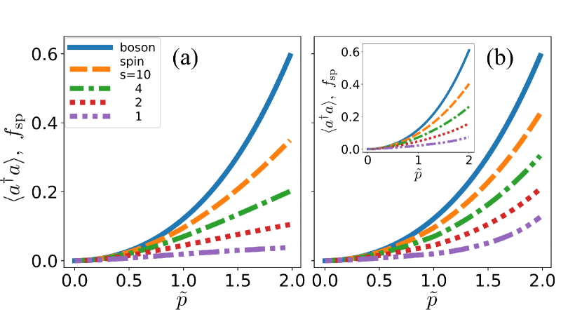
Figure 1: The photon number $\langle\hat{a}^{\dagger}\hat{a}\rangle$ of the ground state of a KPO as a function of $\tilde{p}$ and the corresponding function $f_{\text{sp}}=s-\langle\hat{s}^{x}\rangle$ of the spin models for (a) $\alpha=0$, (b) $\alpha=\alpha_{c}$, and [inset of (b)] $\alpha^{2}$ equal to the exact $\langle\hat{a}^{\dagger}\hat{a}\rangle$. Both the two panels display the same photon number (solid). The curves for the spin models are for $s=1$ (dashed double dotted), 2 (dotted), 4 (dashed dotted), and 10 (dashed). All the systems are for $\tilde{\Delta}=1$ and $\tilde{\epsilon}=0$.

Figure 1 (a) shows the photon number $\langle\hat{a}^{\dagger}\hat{a}\rangle$ as a function of $\tilde{p}$ for $\tilde{\Delta}=1$ and $\tilde{\epsilon}=0$ and the corresponding function

$$f_{\text{sp}}=s-\langle\hat{s}^{x}\rangle$$ (26)

of the spin models for $\alpha=0$ and $s=1$, 2, 4, and 10. $f_{\text{sp}}$ is close to $\langle\hat{a}^{\dagger}\hat{a}\rangle$ at small $\tilde{p}$. The difference appears and grows with $\tilde{p}$, but $f_{\text{sp}}$ captures the trend of $\langle\hat{a}^{\dagger}\hat{a}\rangle$. $f_{\text{sp}}$ for larger $s$ shows smaller deviations from $\langle\hat{a}^{\dagger}\hat{a}\rangle$. $f_{\text{sp}}$ for $\alpha=\alpha_{c}$ and equal to the exact $\sqrt{\langle\hat{a}^{\dagger}\hat{a}\rangle}$ are shown in Fig. 1 (b) and its inset. The model with $\alpha=\alpha_{c}$ suppresses the deviation of $f_{\text{sp}}$ from $\langle\hat{a}^{\dagger}\hat{a}\rangle$ more than the one with $\alpha=0$ and behaves like the one with $\alpha$ equal to the exact $\sqrt{\langle\hat{a}^{\dagger}\hat{a}\rangle}$.

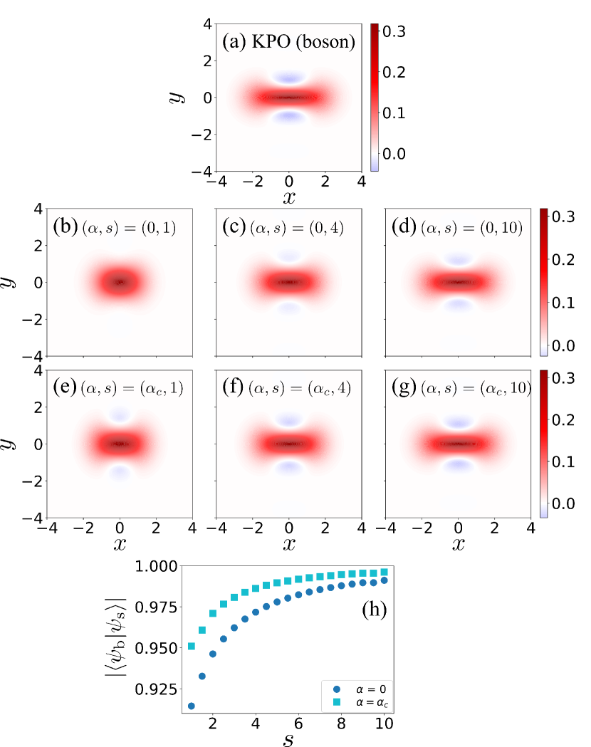
Figure 2: The Wigner function of the ground state of (a) a KPO and the corresponding function of the spin models for (b) $(\alpha,s)=(0,1)$, (c) $(0,4)$, (d) $(0,10)$, (e) $(\alpha_{c},1)$, (f) $(\alpha_{c},4)$, and (g) $(\alpha_{c},10)$. $x$ and $y$ denote $\sqrt{2}\text{Re}(\alpha)$ and $\sqrt{2}\text{Im}(\alpha)$ for a coherent state $|\alpha\rangle$, respectively. (h) The overlap $|\langle\psi_{\text{b}}|\psi_{\text{s}}\rangle|$ of bosonic and spin ground states as a function of $s$ for $\alpha=0$ (circle) and $\alpha_{c}$ (square). All the systems are for $\tilde{\Delta}=1$, $\tilde{p}=2$ and $\tilde{\epsilon}=0$.

Figure 2 (a) shows the Wigner function [44] of the ground state of a KPO for $\tilde{\Delta}=1$, $\tilde{p}=2$, and $\tilde{\epsilon}=0$. The shape of the region for positive values shows a sign of bifurcation. The function also has negative values that is the evidence of quantum superposition. In order to calculate the corresponding function of the spin models, we replace the density matrix of the KPO with that of the spin models. Negative values are not clearly found in the resulting function for $\alpha=0$ and $s=1$ [Fig. 2 (b)], while they are found for larger $s$ [Figs. 2 (c) and (d)]. The spin model with $\alpha=\alpha_{c}$ takes negative values for $s=1$ [Fig. 2 (e)]. As $s$ increases [Figs. 2 (f) and (g)], the positive-value region is squeezed, and the function becomes more similar to that of the bosonic model. The function similarity is quantified by the state overlap $|\langle\psi_{\text{b}}|\psi_{\text{s}}\rangle|$, where $|\psi_{\text{b}}\rangle$ and $|\psi_{\text{s}}\rangle$ denote the ground states of bosonic and spin models, respectively. We define the overlap by

$$|\langle\psi_{\text{b}}|\psi_{\text{s}}\rangle|=\left|\sum_{n=0}^{2s}\langle\psi_{\text{b}}|n\rangle{}_{x}\langle s-n,s|\psi_{\text{s}}\rangle\right|,$$ (27)

where $\hat{a}^{\dagger}\hat{a}|n\rangle=n|n\rangle$ and $\hat{s}^{x}|s-n,s\rangle_{x}=(s-n)|s-n,s\rangle_{x}$. Figure 2 (h) demonstrates that the overlap for $\alpha=\alpha_{c}$ increases with $s$ and is always larger than that for $\alpha=0$. Note that the Wigner function for $s=1/2$ does not show squeezing and the negative-value region (not shown), since the nonlinear terms in the Hamiltonian become constants when $s=1/2$.

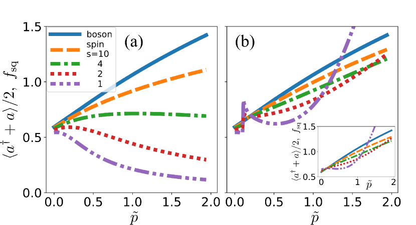
Figure 3: The quadrature amplitude $\langle\hat{a}^{\dagger}+\hat{a}\rangle/2$ of the ground state of a KPO as a function of $\tilde{p}$ and the corresponding function $f_{\text{sq}}=(2s-\alpha^{2})^{-1/2}\langle\hat{s}^{z}\rangle$ of the spin model [Eq. (18)] for (a) $\alpha=0$, (b) $\alpha=\alpha_{c}$, and [inset of (b)] $\alpha^{2}$ equal to the exact $\langle\hat{a}^{\dagger}\hat{a}\rangle$. Both the two panels display the same quadrature amplitude (solid). The curves for the spin models are for $s=1$ (dashed double dotted), 2 (dotted), 4 (dashed dotted), and 10 (dashed). All the systems are for $\tilde{\Delta}=0$ and $\tilde{\epsilon}=0.1$.

We also investigate the systems with coherent driving $\epsilon$, where the quadrature amplitude $\langle\hat{a}^{\dagger}+\hat{a}\rangle/2$ can have a finite value. Figure 3 (a) shows $\langle\hat{a}^{\dagger}+\hat{a}\rangle/2$ as a function of $\tilde{p}$ for $\tilde{\Delta}=0$ and $\tilde{\epsilon}=0.1$ and the corresponding function

$$f_{\text{sq}}=\frac{\langle\hat{s}^{z}\rangle}{\sqrt{2s-\alpha^{2}}}$$ (28)

of the spin models for $\alpha=0$ and $s=1$, 2, 4, and 10. The curves of $f_{\text{sq}}$ largely deviate from the curve of $\langle\hat{a}^{\dagger}+\hat{a}\rangle/2$ except for $\tilde{p}\simeq 0$. We find in Fig. 3 (b) that $f_{\text{sq}}$ for $\alpha=\alpha_{c}$ and $s\geq 2$ do not have such a large difference even at large $p$, but that for $s=1$ has a steep peak at $\tilde{p}\simeq 0.1$ caused by the discontinuous change in $\alpha_{c}$ at $\tilde{p}=\tilde{\Delta}+\tilde{\epsilon}$, which is more accentuated in $1-\alpha^{2}/2s$ for smaller $s$. The similar curves, but without the steep peak, are obtained from the models with $\alpha$ equal to the exact $\sqrt{\langle\hat{a}^{\dagger}\hat{a}\rangle}$ [inset of Fig. 3 (b)]. The result demonstrates that the transformation based on the expansion with $\alpha_{c}$ gives pretty good spin models that can describe physical quantities of a KPO at least qualitatively.

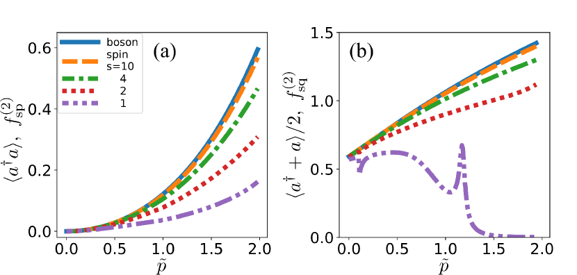
Figure 4: (a) The photon number $\langle\hat{a}^{\dagger}\hat{a}\rangle$ and (b) quadrature amplitude $\langle\hat{a}^{\dagger}+\hat{a}\rangle/2$ of the ground state of a KPO as a function of $\tilde{p}$ and the corresponding functions (a) $f_{\text{sp}}^{(2)}=s-\langle\hat{s}^{x}\rangle$ and (b) $f_{\text{sq}}^{(2)}$ [Eq. (42)] of the spin models including the second order terms [Eq. (46)] for $\alpha=\alpha_{c}$. The solid curves show the results of the KPO. The curves for the spin models are for $s=1$ (dashed double dotted), 2 (dotted), 4 (dashed dotted), and 10 (dashed). $\tilde{\Delta}$ and $\tilde{\epsilon}$ are set to the same as those for (a) Fig. 1 and (b) Fig. 3, i.e., (a) $(\tilde{\Delta},\tilde{\epsilon})=(1,0)$ and (b) (0, 0.1), respectively.

Let us look at the spin models including the second order terms for $\alpha=\alpha_{c}$ that is given in Appendix. We represent the spin counterparts of photon number and quadrature amplitude for this case as $f_{\text{sp}}^{(2)}$ and $f_{\text{sq}}^{(2)}$, respectively. The expression of $f_{\text{sq}}^{(2)}$ is different from $f_{\text{sq}}$ and is given by the right hand side of Eq. (42) in Appendix. As shown in Fig. 4 (a), all the curves of $f_{\text{sp}}^{(2)}$ become closer to $\langle\hat{a}^{\dagger}\hat{a}\rangle$ compared to $f_{\text{sp}}$ [Fig. 1 (b)]. $f_{\text{sq}}^{(2)}$ for $s=4$ and 10 [Fig. 4 (b)] also become closer to $\langle\hat{a}^{\dagger}+\hat{a}\rangle/2$ compared to $f_{\text{sq}}$ [Fig. 3 (b)], but for $s=1$ and 2 show no such improvement. This finding demonstrates that the transforamtion including higher order terms can give more accurate description, but the accuracy is not necessarilly improved for small $s$.

IV.2 Two interacting KPOs

Let us move to interacting KPOs. The simplest case is two KPOs governed by Eq. (3) for $N=2$, $J_{12}=J_{21}=J$, and $\xi_{0}=1$,

$$\hat{H}_{\text{b}}^{(2)}=\hat{H}_{\text{b},1}+\hat{H}_{\text{b},2}-J(\hat{a}^{\dagger}_{1}\hat{a}_{2}+\hat{a}_{1}\hat{a}^{\dagger}_{2}),$$ (29)

where $\hat{H}_{\text{b},i}$ for $i=1$ and 2 are given by Eq. (4). This system is transformed to

$$\hat{H}_{\text{s}}^{(2)}=\hat{H}_{\text{s},1}+\hat{H}_{\text{s},2}-\frac{2J}{2s-\alpha^{2}}\left(\hat{s}^{z}_{1}\hat{s}^{z}_{2}+\hat{s}^{y}_{1}\hat{s}^{y}_{2}\right),$$ (30)

where $\hat{H}_{\text{s},i}$ for $i=1$ and 2 is given by Eq. (18). This spin model is based on the first order terms in the expansion. As mentioned in Sec. III, $\hat{s}^{z}_{1}\hat{s}^{z}_{2}$ might be dominant in the coupling. We also investigate the ground state of

$$\hat{H}^{\prime(2)}_{\text{s}}=\hat{H}_{\text{s},1}+\hat{H}_{\text{s},2}-\frac{2J}{2s-\alpha^{2}}\hat{s}^{z}_{1}\hat{s}^{z}_{2}$$ (31)

to examine the effects of ignoring $\hat{s}^{y}_{1}\hat{s}^{y}_{2}$. We set $\alpha$ to $\alpha_{c}$ for $\tilde{\epsilon}=0$, namely

$$\alpha_{c0}=\sqrt{\tilde{p}-\tilde{\Delta}}\theta(\tilde{p}-\tilde{\Delta}),$$ (32)

where $J$ is not included as well as $\tilde{\epsilon}$. To incorporate the effects of coherent driving and interaction into $\alpha$, we need the sign of quadrature amplitude of the ground state, which is what we aim to obtain with QA. Therefore incorporating those effects is not fit for the purpose of constructing the model, and we adopt $\alpha_{c0}$ in Eq. (32) for $\alpha$. When we investigated a single KPO in Sec. IV.1, we included $\epsilon$ in $\alpha_{c}$, since the sign of quadrature amplitude in that case was trivial.

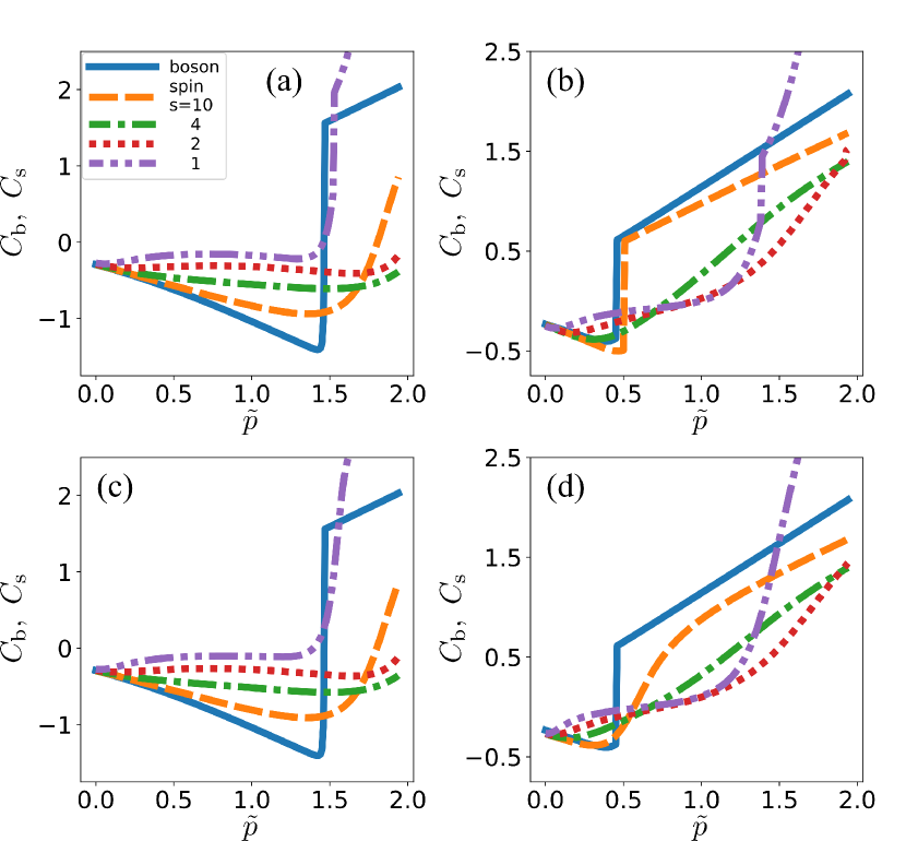
Figure 5: The correlation $C_{\text{b}}=\langle(\hat{a}^{\dagger}_{1}+\hat{a}_{1})(\hat{a}^{\dagger}_{2}+\hat{a}_{2})\rangle/4$ of quadrature amplitude of the ground state of two KPOs as a function of $\tilde{p}$ and the corresponding function $C_{\text{s}}=\langle\hat{s}^{z}_{1}\hat{s}^{z}_{2}\rangle/(2s-\alpha_{c0}^{2})$ of the spin models for $\alpha=\alpha_{c0}$. $C_{\text{s}}$ shown in (a) and (b) is calculated for $\hat{H}_{\text{s}}^{(2)}$, and in (c) and (d) is for $\hat{H}^{\prime(2)}_{\text{s}}$. $(\tilde{\epsilon}_{1},\tilde{\epsilon}_{2},\tilde{J})$ is set to (a) $(0.1,-0.1,0.08)$, (b) $(0.1,-0.1,0.12)$, (c) $(0.1,-0.1,0.08)$, and (d) $(0.1,-0.1,0.12)$. The curves for the spin models are for $s=1$ (dashed double dotted), 2 (dotted), 4 (dashed dotted), and 10 (dashed). $\tilde{\Delta}=0$ in all the systems.

We focus on the correlation of quadrature amplitude of KPOs,

$$C_{\text{b}}=\frac{1}{4}\left\langle\left(\hat{a}^{\dagger}_{1}+\hat{a}_{1}\right)\left(\hat{a}^{\dagger}_{2}+\hat{a}_{2}\right)\right\rangle,$$ (33)

and the corresponding function of the spin models

$$C_{\text{s}}=\frac{\langle\hat{s}^{z}_{1}\hat{s}^{z}_{2}\rangle}{2s-\alpha_{c0}^{2}}.$$ (34)

Figure 5 shows $C_{\text{b}}$ and $C_{\text{s}}$ for $\tilde{\epsilon}_{1}=0.1$, $\tilde{\epsilon}_{2}=-0.1$, and $\tilde{J}=J/K=0.08$ and 0.12. $C_{\text{b}}$ and $C_{\text{s}}$ at small $\tilde{p}$ take negative values due to the difference in sign of $\tilde{\epsilon}_{1}$ and $\tilde{\epsilon}_{2}$ and shift to positive values at an intermediate $\tilde{p}$. This shift is caused by the change of dominant term from the coherent driving to the coupling. $C_{\text{s}}$ for $\tilde{J}=0.08$ and $s=10$ follows $C_{\text{b}}$, although $C_{\text{s}}$ is more gradual than $C_{\text{b}}$ [Fig. 5 (a)]. $C_{\text{s}}$ for $\tilde{J}=0.12$ and $s=10$ reproduces the shift in $C_{\text{b}}$ [Fig. 5 (b)], which occurs at smaller $\tilde{p}$ than for $\tilde{J}=0.08$. $C_{\text{s}}$ for $s=1,2$, and 4 agree with $C_{\text{b}}$ at small $\tilde{p}$, but they depart from $C_{\text{b}}$ as $\tilde{p}$ increases. Note that it is just a coincidence that the rapid increase of $C_{\text{s}}$ for $\tilde{J}=0.08$ and $s=1$ overlaps $C_{\text{b}}$. We also compute $C_{\text{s}}$ of $\hat{H}^{\prime(2)}_{\text{s}}$, where $\hat{s}^{y}_{1}\hat{s}^{y}_{2}$ is ignored. We find no significant difference between $C_{\text{s}}$ of $\hat{H}_{\text{s}}^{(2)}$ and $\hat{H}^{\prime(2)}_{\text{s}}$ for $\tilde{J}=0.08$ [Fig. 5 (c)], while $C_{\text{s}}$ of $\hat{H}^{\prime(2)}_{\text{s}}$ for $\tilde{J}=0.12$ deviates from that of $\hat{H}_{\text{s}}^{(2)}$ around $\tilde{p}$ where $C_{\text{b}}$ shifts to positive values [Fig. 5 (d)]. It is natural that differences appear in rapid changes of the function at small $\tilde{p}$, since $\hat{s}^{z}_{1}\hat{s}^{z}_{2}$ is expected to be dominant only at large $\tilde{p}$. Figure 5 demonstrates that $C_{\text{s}}$ agrees with $C_{\text{b}}$ at small $\tilde{p}$, while the gap between $C_{\text{b}}$ and $C_{\text{s}}$ grows with $\tilde{p}$, but $C_{\text{s}}$ begins increasing and exhibits the similar trend to $C_{\text{b}}$ at large $\tilde{p}$. The larger $s$ is, the larger range of $\tilde{p}$ over which our spin model can describe KPOs well. In addition, $\hat{H}^{\prime(2)}_{\text{s}}$ is a good approximation of $\hat{H}_{\text{s}}^{(2)}$, except for the rapid changes at small $\tilde{p}$. Importantly, we can extract the correct sign of correlations of the two KPOs, which corresponds to the Ising spin configuration in QA, from our spin models at large $\tilde{p}$.

IV.3 Mean-field model

We investigate the mean-field models to effectively find the collective behavior. The mean-field model of KPOs with a coupling constant $J$ is

$$\hat{H}_{\text{b}}^{\text{mf}}=\hat{H}_{\text{b}}-Jx\left(\hat{a}^{\dagger}+\hat{a}\right)-iJy\left(\hat{a}^{\dagger}-\hat{a}\right),$$ (35)

where $\hat{H}_{\text{b}}$ is given by Eq. (1). The coordination number is included in $J$. $x$ and $y$ are the real and imaginary parts, respectively, of $a$ that is determined by the self-consistent equation,

$$a=\langle\psi_{\text{b}}(a)|\hat{a}|\psi_{\text{b}}(a)\rangle$$ (36)

where $|\psi_{\text{b}}(a)\rangle$ is the ground state of $\hat{H}_{\text{b}}^{\text{mf}}$ for $a$. When $\tilde{p}=0$, we can find the ground states that break the symmetry in $\hat{H}_{\text{b}}^{\text{mf}}$ for $\tilde{p}=0$ involving a transformation $\hat{a}\to\hat{a}e^{i\phi}$ with an arbitrary real $\phi$. When analyzing such states, it is sufficient to consider only the ground state with $x\geq 0$ and $y=0$. When $\tilde{p}>0$, the pump suppresses $y$, and thus $y=0$. We therefore simplify the Hamiltoinan as

$$\hat{H}_{\text{b}}^{\text{mf}}=\hat{H}_{\text{b}}-Jx\left(\hat{a}^{\dagger}+\hat{a}\right).$$ (37)

The corresponding mean-field spin model is

$$\hat{H}_{\text{s}}^{\text{mf}}=\hat{H}_{\text{s}}-\frac{2J}{2s-\alpha^{2}}m^{z}\hat{s}^{z},$$ (38)

where $\hat{H}_{\text{s}}$ is given by Eq. (18), and $m^{z}$ is determined by

$$m^{z}=\langle\psi_{\text{s}}(m^{z})|\hat{s}^{z}|\psi_{\text{s}}(m^{z})\rangle$$ (39)

for the ground state $|\psi_{\text{s}}(m^{z})\rangle$ of $\hat{H}_{\text{s}}^{\text{mf}}$ for $m^{z}$. We set $\alpha=\alpha_{c0}$ in Eq. (32). When we solve the self-consistent equations recursively, the initial values of $x$ and $m^{z}$ are set to tiny positive ones to focus on the solutions for $x\geq 0$ and $m^{z}\geq 0$. We do not discuss the validity of the mean-field approximation to describe many interacting KPOs. That is beyond the scope of this paper.

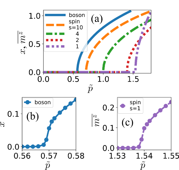
Figure 6: (a) The expectation value $x$ of quadrature amplitude of the ground state of the mean-field model for KPOs as a function of $\tilde{p}$ (solid) and the corresponding function $\overline{m^{z}}$ of the mean-field spin models for $\alpha=\alpha_{c0}$ and $s=1$ (dashed double dotted), 2 (dotted), 4 (dashed dotted), and 10 (dashed). The closeups of the onset of (b) $x$ and (c) $\overline{m^{z}}$ for $s=1$ are also shown. All the systems are for $\tilde{\Delta}=0.4$, $\tilde{\epsilon}=0$, and $\tilde{J}=0.2$.

Both the expectation value $x$ of quadrature amplitde and its spin counterpart $\overline{m^{z}}=(2s-\alpha^{2})^{-1/2}m^{z}$ for small $\tilde{\Delta}$ rise continuously from 0 as $\tilde{p}$ increases [Figs. 6 (a)–(c)]. The onset of $x$ or $\overline{m^{z}}$ can be interpreted as the continuous phase transition from the paramagnetic phase to the ferromagnetic phase. The bifurcation induced by increasing $\tilde{p}$ underlies this phase transition. The spin systems have similar magnetization curves to that of the bosonic system, although the critical points are shifted.

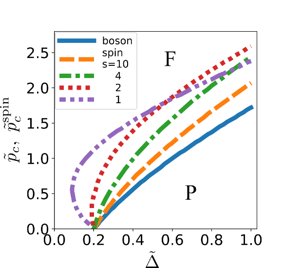
Figure 7: The critical pump amplitude $\tilde{p}_{c}$ of the ground state of the mean-field model for KPOs as a function of $\tilde{\Delta}$ (solid) and the corresponding function $\tilde{p}_{c}^{\text{spin}}$ of the mean-field spin models for $\alpha=\alpha_{c0}$ and $s=1$ (dashed double dotted), 2 (dotted), 4 (dashed dotted), and 10 (dashed). The curves correspond to the phase boundaries between the paramagnetic (P) and ferromagnetic (F) phases. All the systems are for $\tilde{\epsilon}=0$ and $\tilde{J}=0.2$.

The critical points $\tilde{p}_{c}$ and $\tilde{p}_{c}^{\text{spin}}$ of the bosonic and spin systems as a function of $\tilde{\Delta}$ for $\tilde{J}=0.2$ are shwon in Fig. 7. The bosonic system for smaller $\tilde{\Delta}$ than 0.2, say $\tilde{\Delta}_{c}$, has a finite $x$ even at $\tilde{p}=0$, whereas that for $\tilde{\Delta}>\tilde{\Delta}_{c}$ lies in the paramagnetic phase at $\tilde{p}=0$ and undergoes the phase transition at a finite $\tilde{p}_{c}$. The spin systems for $s=4$ and 10 show similar phase boundaries, although the gap between $\tilde{p}_{c}^{\text{spin}}$ and $\tilde{p}_{c}$ grows as $\tilde{\Delta}$ increases. We also find that the spin systems for $s=1$ and 2 at $\tilde{\Delta}\lesssim\tilde{\Delta}_{c}$ exhibit the reentrant transition. As $\tilde{p}$ is increased, the systems cross the phase boundary twice. Their boundaries for larger $\tilde{\Delta}$, however, show the same trend as that of the KPOs.

V Conclusion

We have presented effective spin-$s$ models of Kerr-nonlinear parametric oscillators (KPOs) for quantum annealing (QA). The detuning and coherent driving work as transverse and longitudinal fields in the spin systems, respectively. The Kerr effect and the parametric driving turn to the nonlinear terms of $\hat{s}^{x}$ and $\hat{s}^{z}$, respectively. Although we truncate the expansion in the transformation, the spin models, in particular, for large $s$ at small $\tilde{p}$ show good correspondence to the bosonic model. Even when $s$ is small but larger than 1/2, the spin models partially capture features of KPOs, e.g., bifurcation and phase transitions. As the photon number of KPOs becomes large, the gap between the spin and bosonic models grows, but setting a parameter $\alpha$ to an approximate value of $\sqrt{\langle\hat{a}^{\dagger}\hat{a}\rangle}$ makes the gap smaller. The gap can be also reduced by including higher order terms in the transformation.

The spin models presented in this paper are simple but qualitatively reproduce KPOs and clarify roles of parameters of KPOs in QA. We expect that the models will help us understand the behavior of KPOs, in particular, when comparing QA with KPOs to conventional QA based on the transverse-field Ising model. Improvements in quantitative accuracy would increase the usefulness of the method, but that is a topic for future work.

*

Appendix A Transformation with the second term in Eq. (13)

Equation (13) reads

$$\hat{s}^{z}= \sqrt{2s-\alpha^{2}}\frac{\hat{a}^{\dagger}+\hat{a}}{2}$$ (40)

$$-\frac{1}{4\sqrt{2s-\alpha^{2}}}\bigg{[}\hat{a}^{\dagger}\hat{a}\frac{\hat{a}^{\dagger}+\hat{a}}{2}+\frac{\hat{a}^{\dagger}+\hat{a}}{2}\hat{a}^{\dagger}\hat{a}$$

$$-\left(1+\alpha^{2}\right)\frac{\hat{a}^{\dagger}+\hat{a}}{2}\bigg{]}+\cdots.$$

We assume that $(\hat{a}^{\dagger}+\hat{a})/2$ is represented as $\hat{s}^{z}/\sqrt{2s-\alpha^{2}}+A_{1}$, where $\hat{s}^{z}/\sqrt{2s-\alpha^{2}}$ is obtained from the transformation that only takes into account the first term in Eq. (40). We substitute $\hat{s}^{z}/\sqrt{2s-\alpha^{2}}+A_{1}$ into $(\hat{a}^{\dagger}+\hat{a})/2$ in Eq. (40) including up to the second term and ignore terms such as $A_{1}/\sqrt{2s-\alpha^{2}}$ to obtain

$$A_{1}=\frac{(2s-1-2\alpha^{2})\hat{s}^{z}-\hat{s}^{x}\hat{s}^{z}-\hat{s}^{z}\hat{s}^{x}}{4(2s-\alpha^{2})^{3/2}}$$ (41)

and

$$\frac{\hat{a}^{\dagger}+\hat{a}}{2}= \left[\frac{5}{4\sqrt{2s-\alpha^{2}}}-\frac{1+\alpha^{2}}{4(2s-\alpha^{2})^{3/2}}\right]\hat{s}^{z}$$ (42)

$$-\frac{\hat{s}^{x}\hat{s}^{z}+\hat{s}^{z}\hat{s}^{x}}{4(2s-\alpha^{2})^{3/2}},$$

where the higher order terms in powers of $1/(2s-\alpha^{2})$ are dropped. Equation (13) also leads to

$$(\hat{s}^{z})^{2}= \frac{2s-\alpha^{2}}{2}\left(\frac{\hat{a}^{\dagger 2}+\hat{a}^{2}}{2}+\hat{a}^{\dagger}\hat{a}+\frac{1}{2}\right)$$ (43)

$$-\bigg{[}\frac{(\hat{a}^{\dagger}\hat{a})^{2}}{2}+\left(\hat{a}^{\dagger}\hat{a}\frac{\hat{a}^{\dagger 2}+\hat{a}^{2}}{2}+\frac{\hat{a}^{\dagger 2}+\hat{a}^{2}}{2}\hat{a}^{\dagger}\hat{a}\right)$$

$$-\frac{1+2\alpha^{2}}{4}\frac{\hat{a}^{\dagger 2}+\hat{a}^{2}}{2}-\frac{\alpha^{2}}{2}\hat{a}^{\dagger}\hat{a}-\frac{\alpha^{2}}{4}\bigg{]}+\cdots.$$

We substitute $-s+\hat{s}^{x}-1/2+2(\hat{s}^{z})^{2}/(2s-\alpha^{2})+B_{1}$ into $(\hat{a}^{\dagger 2}+\hat{a}^{2})/2$ in Eq. (43), where $-s+\hat{s}^{x}-1/2+2(\hat{s}^{z})^{2}/(2s-\alpha^{2})$ is obtained from the transformation that only takes into account the first line in Eq. (43). We also ignore terms such as $B_{1}/(2s-\alpha^{2})$ to obtain

$$B_{1}= \frac{(2s-1-2\alpha^{2})(\hat{s}^{z})^{2}-\hat{s}^{x}(\hat{s}^{z})^{2}-(\hat{s}^{z})^{2}\hat{s}^{x}}{(2s-\alpha^{2})^{2}}$$ (44)

$$+\frac{1}{4(2s-\alpha^{2})}$$

and

$$\frac{\hat{a}^{\dagger 2}+\hat{a}^{2}}{2}= -s+\hat{s}^{x}-\frac{1}{2}+\left[\frac{3}{2s-\alpha^{2}}-\frac{1+\alpha^{2}}{(2s-\alpha^{2})^{2}}\right](\hat{s}^{z})^{2}$$ (45)

$$+\frac{1}{4(2s-\alpha^{2})}-\frac{\hat{s}^{x}(\hat{s}^{z})^{2}+(\hat{s}^{z})^{2}\hat{s}^{x}}{(2s-\alpha^{2})^{2}},$$

where the higher order terms in powers of $1/(2s-\alpha^{2})$ are dropped. Equations (14), (15) (42), and (45) are used to transform the Hamiltonian for a KPO [Eq. (1)] to

$$\hat{H}_{\text{spin}}= -\left[\frac{3}{2s-\alpha^{2}}-\frac{1+\alpha^{2}}{(2s-\alpha^{2})^{2}}\right]p(\hat{s}^{z})^{2}$$ (46)

$$-\left[\Delta+p+\left(s-\frac{1}{2}\right)K\right]\hat{s}^{x}+\frac{K}{2}(\hat{s}^{x})^{2}$$

$$-\left[\frac{5}{2\sqrt{2s-\alpha^{2}}}-\frac{1+\alpha^{2}}{2(2s-\alpha^{2})^{3/2}}\right]\epsilon\hat{s}^{z}$$

$$+\frac{\epsilon}{2(2s-\alpha^{2})^{3/2}}\left(\hat{s}^{x}\hat{s}^{z}+\hat{s}^{z}\hat{s}^{x}\right)$$

$$+\frac{p}{(2s-\alpha^{2})^{2}}\left[\hat{s}^{x}(\hat{s}^{z})^{2}+(\hat{s}^{z})^{2}\hat{s}^{x}\right].$$