STaR: Knowledge Graph Embedding by Scaling, Translation and Rotation

Abstract

The bilinear method is mainstream in Knowledge Graph Embedding (KGE), aiming to learn low-dimensional representations for entities and relations in Knowledge Graph (KG) and complete missing links. Most of the existing works are to find patterns between relationships and effectively model them to accomplish this task. Previous works have mainly discovered 6 important patterns like non-commutativity. Although some bilinear methods succeed in modeling these patterns, they neglect to handle 1-to-N, N-to-1, and N-to-N relations (or complex relations) concurrently, which hurts their expressiveness. To this end, we integrate scaling, the combination of translation and rotation that can solve complex relations and patterns, respectively, where scaling is a simplification of projection. Therefore, we propose a corresponding bilinear model Scaling Translation and Rotation (STaR) consisting of the above two parts. Besides, since translation can not be incorporated into the bilinear model directly, we introduce translation matrix as the equivalent. Theoretical analysis proves that STaR is capable of modeling all patterns and handling complex relations simultaneously, and experiments demonstrate its effectiveness on commonly used benchmarks for link prediction.

1 Introduction

Knowledge Graph (KG), storing data as triples like (head entity, relation, tail entity), is a growing way to deal with relational data. It has attracted the attention of researchers in recent years due to its applications in boosting other fields such as question answering (Mohammed, Shi, and Lin 2018), recommender systems (Zhang et al. 2016), and natural language processing (Wang et al. 2017; Ji et al. 2021).

Since KG is usually incomplete, it needs to be completed by predicting the missing edges. A popular and effective way to accomplish this task is Knowledge Graph Embedding (KGE), which aims to find appropriate low-dimensional representations for entities and relations.

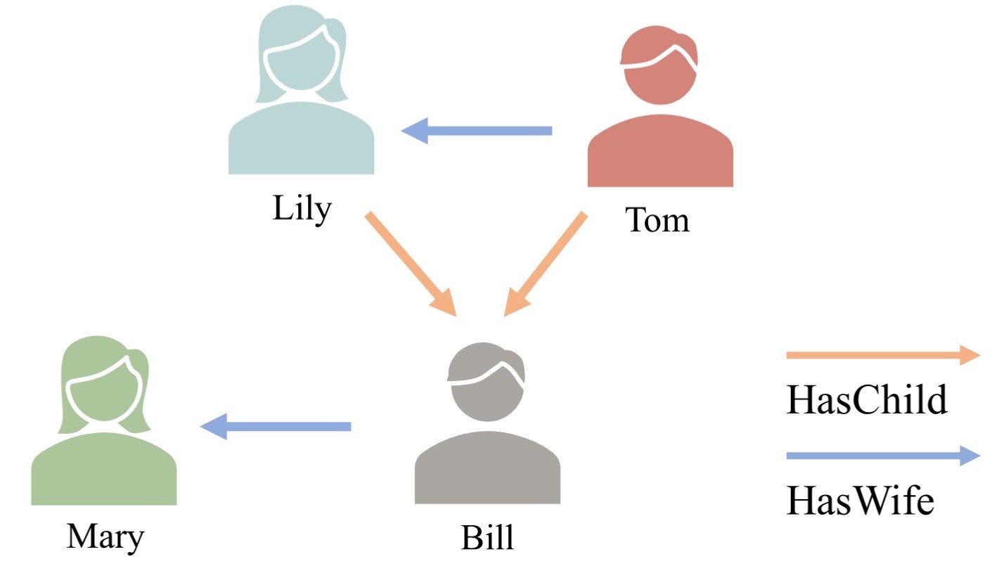
(a) Complex relations and non-commutativity pattern

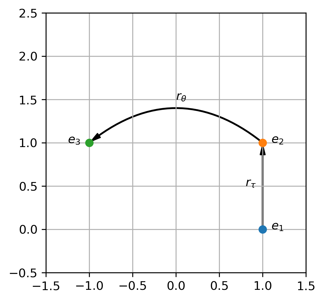
(b) Translate then rotate

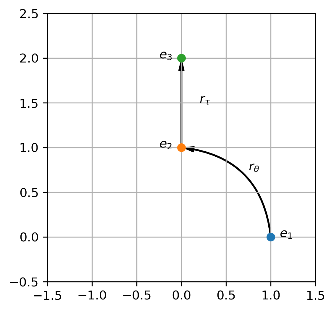
(c) Rotate then translate

Figure 1: Figure 1(a) gives examples of N-to-1 relation and non-commutativity pattern. Figure 1(b) and Figure 1(c) show how translation and rotation model non-commutativity patterns.

A mainstream of KGE is the bilinear method, which uses the product of entities and relations as a similarity. While two major problems in KGE are how to model different relation patterns and how to handle 1-to-N, N-to-1, and N-to-N relations (or complex relations) (Sun et al. 2019; Wang et al. 2014; Lin et al. 2015). For the first problem, previous studies have mainly discovered 6 patterns (Sun et al. 2019; Xu and Li 2019; Yang, Sha, and Hong 2020). For example, as shown in Figure 1(a), HasChild and HasWife form a non-commutativity pattern, since the child of Tom’s wife is Bill while the wife of Tom’s child is Mary. For the second problem, we take an N-to-1 relation HasChild as an example illustrated in the same figure, in which Bill is the child of both Lily and Tom.

Although some recent works have successfully modeled different relation patterns, they neglect to handle complex relations concurrently. To be more specific, they represent relations as rotations (or reflections) to model different patterns like DihEdral (Xu and Li 2019) and QuatE (Zhang et al. 2019), yet ignore that naive rotation is just like translation in TransE(Bordes et al. 2013), which is difficult to handle complex relations.

To this end, we borrow the ideas from distance-based methods to go beyond rotation and solve these two problems simultaneously. Specifically, we combine projection that handles complex relations (Wang et al. 2014; Lin et al. 2015) and the combination of translation and rotation that models relation patterns (Chami et al. 2020), e.g. we demonstrate how they model non-commutativity in Figure 1(b) and Figure 1(c). Thus, we propose a corresponding bilinear model Scaling Translation and Rotation (STaR), where scaling is a simplification of projection and translation is introduced as matrix widely used in Robotics (Paul 1981). STaR can model different patterns and handle complex relations concurrently, and takes linear rather than quadratic parameters to embed a relation efficiently. Comparing to previous bilinear models, STaR is closest to ComplEx (Trouillon et al. 2016), which is equivalent to the combination of rotation and scaling and will be compared in Section 5 minutely.

Experiments on different settings demonstrate the effectiveness of our model against previous ones, while elaborated analysis against ComplEx shows the changes brought about by translation and verifies that our model improves from modeling the non-commutativity pattern. The main contributions of this paper are as follows:

1. We propose a bilinear model STaR that can efficiently model relation patterns and handle complex relations concurrently.

2. To the best of our knowledge, this is the first work introducing translation to the bilinear model, which brings new modules to it and connect with distance-based methods.

3. The proposed STaR achieves comparable results on three commonly used benchmarks for link prediction.

2 Related Work

Generally speaking, previous works on KGE can be divided into bilinear, distance-based, and other methods.

Bilinear Methods

Bilinear Methods measure the similarity of head and tail entities by their inner product under a relation specific transformation represented by a matrix $R$. RESCAL (Nickel, Tresp, and Kriegel 2011) is the ancestor of all bilinear models, whose $R$ is arbitrary and has $n^{2}$ parameters. RESCAL is expressive yet ponderous and tends to overfit. To alleviate this issue, DistMult (Yang et al. 2015) uses diagonal matrices and reduces $n^{2}$ to $n$. ComplEx (Trouillon et al. 2016) transforms DistMult into complex spaces to model anti-symmetry pattern. Analogy (Liu, Wu, and Yang 2017) considers analogical pattern, which is equivalent to commutativity pattern, and generalizes DistMult, ComplEx, and HolE (Nickel, Rosasco, and Poggio 2016). Although these descendants are powerful in handling complex relations and some patterns, they fail to model non-commutativity patterns.

The non-commutativity pattern was proposed by DihEdral (Xu and Li 2019) which uses a dihedral group to model all patterns. Besides, this pattern can also be modeled by hypercomplex values like quaternion or octonion used in QuatE (Zhang et al. 2019). Although they succeed in modeling non-commutativity, they are poor at handling complex relations. Thus, none of the previous bilinear methods has intended to handle relations and model concurrently.

Distance-Based Methods

In contrast, Distance-Based Methods use distance to measure the similarity. TransE (Bordes et al. 2013) inspired by word2vec (Mikolov et al. 2013) proposes the first distance-based model and model relation as translation. TransH (Wang et al. 2014), TransR (Lin et al. 2015) find that TransE is incapable to model complex relations like part_of and fix this problem by projecting entities into relation-specific hyperspaces.

RotatE (Sun et al. 2019) utilizes rotation to model inversion and other patterns. Due to its success, subsequent models adopt the idea of rotation. HAKE (Zhang et al. 2020a) argues that rotation is incompetent to model hierarchical structures and introduces a radial part. MuRE (Balazevic, Allen, and Hospedales 2019a) incorporates rotation with scaling while RotE (Chami et al. 2020) combines rotation and translation. Besides, they also have hyperbolic versions as MuRP and RotH. PairRE (Chao et al. 2021) also tries to model both the problems of patterns and complexity together, yet neglects the non-commutativity pattern.

Other Methods

Apart from the above two, some studies also employ black boxes or external information. ConvE (Dettmers et al. 2018) and ConKB (Nguyen et al. 2018) utilize convolution neural network while R-GCN (Schlichtkrull et al. 2018) and RGHAT (Zhang et al. 2020b) apply graph neural networks. Besides, some other works use external information like text (An et al. 2018; Yao, Mao, and Luo 2019), while they are out of our consideration.

Besides specific models, other researchers believe that some previous models are limited by overfitting. Thus, they propose better regularization terms like N3 (Lacroix, Usunier, and Obozinski 2018) and DURA (Zhang, Cai, and Wang 2020) to handle this problem.

Table 1: The score function and ability to model relation patterns of several models.

		Relation Patterns						Performance on
Model	Score Function	Composition	Symmetry	Anti-Symmetry	Commutativity	Non-Commutativity	Inversion	Complex Relations
TransE	$-\|h+r-t\|$	✓	✗	✓	✓	✗	✓	Low
TransR	$-\|M_{r}h+r-M_{r}t\|$	✓	✓	✓	✓	✓	✓	High
RotatE	$-\|h\circ r-t\|$	✓	✓	✓	✓	✗	✓	Low
MuRE	$-\|\rho\circ h+r-t\|$	✓	✓	✓	✓	✓	✓	Low
RotE	$-\|hRot(\theta_{r})+r-t\|$	✓	✓	✓	✓	✓	✓	Low
DistMult	$h^{T}\text{diag}(r)t$	✓	✓	✗	✓	✗	✓	High
ComplEx	$\text{RE}(h^{T}\text{diag}(r)\bar{t})$	✓	✓	✓	✓	✗	✓	High
QuatE	$Q_{h}\otimes W_{r}^{\triangleleft}\cdot Q_{t}$	✓	✓	✓	✓	✓	✓	Low
STaR	$\hat{h}^{T}R_{*}\hat{t}$	✓	✓	✓	✓	✓	✓	High

3 Methodology

In this section, we will first introduce the background knowledge. Then, we will propose our model STaR by combining the useful modules that solve patterns and complex relations. Finally, we will discuss the translation in the bilinear model.

3.1 Background Knowledge

Knowledge graph

Given an entity set $\mathcal{E}$ and a relation set $\mathcal{R}$, A knowledge graph $\mathcal{T}={(h_{i},r_{j},t_{k})}\subset\mathcal{E}\times\mathcal{R}\times\mathcal{E}$ is a set of triples, where $h_{i}$, $r_{j}$, $t_{k}$, denotes the head entity, relation and tail entity respectively. The number of entities and relations are indicated by $|\mathcal{E}|$and $|\mathcal{R}|$.

Problem definition

Knowledge graph embedding aims to learn a score function $s(h,r,t)$ and the embeddings of entities and relations, which uses the link prediction task to evaluate the performance. Link prediction first splits triples of the knowledge graph $\mathcal{T}$ into train set $\mathcal{T}_{train}$, test set $\mathcal{T}_{test}$ and valid set $\mathcal{T}_{valid}$. Then, for each specific triple in $\mathcal{T}_{test}$, link prediction aims to give the correct entity $tail\in\mathcal{E}$ a lower rank than other candidates given the query $(head,relation,?)$ or head entity $head\in\mathcal{E}$ given the query $(?,relation,tail)$ by utilizing the score function.

Complex relations

The complex relations are defined by tails per head and heads per tail of a relation $r$ (tphr and hptr) (Wang et al. 2014). If tphr $>$ 1.5 and hptr $<$ 1.5 then $r$ is 1-to-N while tphr $>$ 1.5 and hptr $>$ 1.5 means $r$ corresponds to N-to-N.

Relation patterns

Relation patterns are the inherent semantic characteristics of relations, which are helpful to model relations and inference.

Previous works have mainly proposed 6 patterns (Xu and Li 2019; Yang, Sha, and Hong 2020). They are Composition (e.g., my father’s brother is my uncle), Symmetry (e.g., IsSimilarTo), Anti-Symmetry (e.g., IsFatherOf), Commutativity, Non-Commutativity (e.g., my wife’s son is not my son’s wife), Inversion. For the formal definition of all patterns, please refer to Supplementary Material A.

Other notations

We use $h\in\mathbb{R}^{n\times 1}$ and $t\in\mathbb{R}^{n\times 1}$ to denote the embedding of head entity and tail entity respectively, where $n$ is the embedding dimension. And we use $\circ$ to denote the relation composition. For example, if we take $r_{1},r_{2},r_{3}\in\mathcal{R}$, and $r_{3}$ is the composition of $r_{1}$ and $r_{2}$ then $r_{3}=r_{1}\circ r_{2}$.

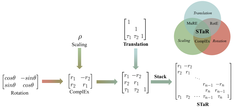
Figure 2: How STaR consists of 3 basic operations and model and related to 3 previous models.

3.2 The Proposed STaR Model

In this part, we will analyze modules in previous works that model different patterns and handle complex relations. Then we will propose a bilinear model Scaling Translation and Rotation (STaR).

In Table 1, we list the score function $s(h,r,t)$ of different models and their ability to model patterns, where we observe that the stickiest one is non-commutativity. To model it, QuatE (Zhang et al. 2019) utilizes quaternion to model the rotation in 3D space. However, we think it is unnecessary to introduce hypercomplex values and redefine the product operator. In contrast, we are inspired by a distance-based model RotE (Chami et al. 2020) that uses the combination of translation and rotation and is capable of modeling non-commutativity in Euclidean spaces as demonstrated in Figure 1(b) and Figure 1(c).

In the same table, we also list the performance of different models on complex relations. From this table, we notice that scaling, as a special case of projection, is helpful for dealing with complex relations (Yang et al. 2015; Trouillon et al. 2016).

Therefore, it seems like we can achieve our goal of modeling patterns and handling complex relations concurrently by assembling the two parts. However, we find that translation is unable to be introduced to the bilinear model directly. To handle this, we introduce a translation matrix widely used in Robotics (Paul 1981) as the equivalent. To show this substitution, we choose a translation $\tau\in\mathbb{R}^{1\times n}$ to a point $x\in\mathbb{R}^{1\times n}$in $\mathbb{R}^{n}$ as an example, and we have:

$$\begin{bmatrix}x\\ 1\end{bmatrix}+\begin{bmatrix}\tau\\ 1\end{bmatrix}=\begin{bmatrix}1&&&\tau_{1}\\ &\ddots&&\vdots\\ &&1&\tau_{n}\\ &&&1\end{bmatrix}\begin{bmatrix}x_{1}\\ \vdots\\ x_{n}\\ 1\end{bmatrix},$$ (1)

where the matrix is the translation matrix.

Finally, we achieve the proposed Scaling Tanslation and Rotation (STaR) model by combing such three modules and stacking these elementary blocks as demonstrated in Figure 2, where ComplEx can be treated as the combination of rotation and scaling in two dimensions manner.

The representation of a relation is thus achieved by assembling a ComplEx matrix with a translation offset:

$$R_{*}=\begin{bmatrix}R_{c}&\\ \tau^{T}&1\\ \end{bmatrix},$$ (2)

where $R_{c}\in\mathbb{R}^{n\times n}$ and $\tau\in\mathbb{R}^{n\times 1}$ denotes the relation specific ComplEx matrix and translation offset respectively. Besides $R_{c}$ is achieved by a vector $r^{c}\in\mathbb{R}^{n\times 1}$ as:

$$R_{c}=\begin{bmatrix}r^{c}_{1}&-r^{c}_{2}\\ r^{c}_{2}&r^{c}_{1}\\ &&\ddots\\ &&&r^{c}_{n-1}&-r^{c}_{n}\\ &&&r^{c}_{n}&r^{c}_{n-1}\\ \end{bmatrix}.$$ (3)

Therefore, the score function of STaR is:

$$s(h,r,t) =\hat{h}^{T}R_{*}\hat{t},$$ (4)

where $\hat{h}=[h^{T},1]^{T}$ and $\hat{t}=[t^{T},1]^{T}$.

From the score function, STaR is proved to model all 6 patterns and handle complex relations as detailed in Supplementary Material B.

Proposition 1.

STaR can model Symmetry, Anti-Symmetry, Composition, Inversion, Commutativity, and Non-Commutativity and handle complex relations concurrently.

3.3 Discussions

In this part, we will detail what does translation brings to bilinear model and how it helps to model the non-commutativity minutely.

What does translation bring to bilinear model?

We unfold the score function of STaR in Equation (4):

$$s(h,r,t) =\hat{h}^{T}R_{*}\hat{t}$$ (5)

$$=(h^{T}R_{c}+\tau^{T})t+1$$

$$=\underbrace{h^{T}R_{c}t}_{\text{ComplEx}}+\underbrace{\tau^{T}t}_{\text{E}}+1.$$

Except the constant $1$ comes from the extra dimension, the above equation shows that it has two parts: ComplEx and the model E proposed by (Toutanova and Chen 2015). The later part E is the dot product of the relation-specific translation $\tau$ and the candidate tail entity $t$ regardless of the head entity. Therefore, E works like determining whether the tail entity suits the relation. For example, given a relation IsLocatedIn, it is impossible to be a correct triple with a tail entity like Bill or Mary no matter what the head entity is.

How does translation help model non-commutativity?

We take two relations $r_{1},r_{2}\in\mathcal{R}$, whose composited relation $r_{3}=r_{1}\circ r_{2}$ is represented as $R_{*}^{1}\cdot R_{*}^{2}$. Similarly, we unfold the score function of a triple regarding $r_{3}$ as:

$$s(h,r_{3},t)= \hat{h}^{T}R_{*}^{1}\cdot R_{*}^{2}\hat{t}$$ (6)

$$= \left((h^{T}R_{c}^{1}+(\tau^{1})^{T})\cdot R_{c}^{2}+(\tau^{2})^{T}\right)t+1$$

$$= \underbrace{h^{T}(R_{c}^{1}R_{c}^{2})t}_{\text{ComplEx}}+\underbrace{\left((\tau^{1})^{T}R_{c}^{2}+(\tau^{2})^{T}\right)t}_{\text{E}}+1.$$

The E in Equation (5) reappears in Equ.(6). As shown in the Table 1, it is E, per se, helps ComplEx to model the non-commutativity pattern since $(\tau^{1})^{T}R_{c}^{2}+(\tau^{2})^{T}\neq(\tau^{2})^{T}R_{c}^{1}+(\tau^{1})^{T}$.

To better understand the role of E, we take $r_{1}$ as IsWifeOf and $r_{2}$ as IsFatherOf as an example. Then the wife of someone’s father must be a woman, while the father of someone’s wife must be a man, where the order of relations affects which tail entities are fitted.

4 Experiments

In this section, we will introduce the experiment settings and three benchmark datasets and show the comparable results of our model.

Table 2: Link prediction results on different benchmarks (best for $n\in\{200,400,500\}$ . † means the results are taken from  (Chami et al. 2020). Since original paper of DURA (Zhang, Cai, and Wang 2020) conduct on extremely high dimension, here we reimplement ComlEx-DURA and RESCAL-DURA. Best results are in bold while the seconds are underlined. STaR is our full model while TaR excludes scaling.

	WN18RR				FB15K237				YAGO3-10
Model	MRR	Hits@1	Hits@3	Hits@10	MRR	Hits@1	Hits@3	Hits@10	MRR	Hits@1	Hits@3	Hits@10
DistMult†	0.43	0.39	0.44	0.49	0.241	0.155	0.263	0.419	0.34	0.24	0.38	0.54
ConvE†	0.43	0.40	0.44	0.52	0.325	0.237	0.356	0.501	0.44	0.35	0.49	0.62
TuckER†	0.470	0.443	0.482	0.526	0.358	0.266	0.394	0.544	-	-	-	-
QuatE†	0.488	0.438	0.508	0.582	0.348	0.248	0.382	0.550	-	-	-	-
RotatE†	0.476	0.428	0.492	0.571	0.338	0.241	0.375	0.533	0.495	0.402	0.550	0.670
MurP†	0.481	0.440	0.495	0.566	0.335	0.243	0.367	0.518	0.354	0.249	0.400	0.567
RotE†	0.494	0.446	0.512	0.585	0.346	0.251	0.381	0.538	0.574	0.498	0.621	0.711
RotH†	0.496	0.449	0.514	0.586	0.344	0.246	0.380	0.535	0.570	0.495	0.612	0.706
ComplEx-N3†	0.480	0.435	0.495	0.572	0.357	0.264	0.392	0.547	0.569	0.498	0.609	0.701
ComplEx-Fro	0.457	0.427	0.469	0.515	0.323	0.235	0.354	0.497	0.568	0.493	0.613	0.699
TaR-Fro (ours)	0.470	0.438	0.481	0.532	0.325	0.239	0.356	0.501	0.567	0.494	0.610	0.699
STaR-Fro (ours)	0.463	0.431	0.476	0.526	0.324	0.236	0.356	0.501	0.574	0.502	0.617	0.701
RESCAL-DURA	0.496	0.452	0.514	0.575	0.370	0.278	0.406	0.553	0.577	0.501	0.621	0.711
ComplEx-DURA	0.488	0.446	0.504	0.571	0.365	0.270	0.401	0.552	0.578	0.507	0.620	0.704
TaR-DURA (ours)	0.488	0.446	0.503	0.567	0.351	0.257	0.387	0.539	0.578	0.506	0.621	0.707
STaR-DURA (ours)	0.497	0.452	0.512	0.583	0.368	0.273	0.405	0.557	0.585	0.513	0.628	0.713

	WN18RR	FB15K237	YAGO3-10
$|\mathcal{E}|$	40,943	14,541	123,182
$|\mathcal{R}|$	11	237	37
Train	86,835	272,115	1,079,040
Valid	3,034	17,535	5,000
Test	3,134	20,466	5,000
$\Psi$	0.003	0.801	0.838

Table 3: Statistics of three benchmark datasets.

4.1 Experiments Settings

Datasets

We evaluate all models on the three most commonly used datasets, which are WN18RR (Dettmers et al. 2018), FB15K237 (Toutanova and Chen 2015) and YAGO3-10 (Mahdisoltani, Biega, and Suchanek 2015). WN18RR and FB15K237 are the subsets of WordnNet and Freebase, respectively. They are the more challenging version of the previous WN18 and FB15K that suffer from data leakage (Dettmers et al. 2018; Toutanova and Chen 2015). We demonstrate the statistics of these benchmarks in Tabel 3. In particular, we use $\Psi$ to denote the imbalance ratio of the train set, which will be introduced in Section 5.1

Baselines

We compare our method with previous models, which are DistMult (Yang et al. 2015), ConvE (Dettmers et al. 2018), Tucker (Balazevic, Allen, and Hospedales 2019b), QuatE (Zhang et al. 2019), MurP (Balazevic, Allen, and Hospedales 2019a), RotE and RotH (Chami et al. 2020) and some previous bilinear models with N3 (Lacroix, Usunier, and Obozinski 2018) and DURA (Zhang, Cai, and Wang 2020) regularization terms. Besides, we also propose TaR consisting of Translation and Rotation for comparison.

Evaluation metrics

We use the score functions to rank the correct tail (head) among all possible candidate entities. Following previous works, we use mean reciprocal rank (MRR) and Hits@$K$ as evaluation metrics. MRR is the mean of the reciprocal rank of valid entities, avoiding the problem of mean rank (MR) being sensitive to outliers. Hits@$K$ ($K\in\{1,3,10\}$ measures the proportion of proper entities ranked within the top $K$. Besides, we follow the filtered setting (Bordes et al. 2013) which ignores those also correct candidates in ranking.

Optimization

Following (Lacroix, Usunier, and Obozinski 2018), we use the cross-entropy loss and the reciprocal setting that adds a reciprocal relation $\tilde{r}$ for each relation $r\in\mathcal{R}$ and $(t,\tilde{r},h)$ for each triple $(h,r,t)\in\mathcal{T}$:

$$\mathcal{L}=-\sum_{(h,r,t)\in\mathcal{T}_{train}}( {\frac{\exp(s(h,r,t))}{\sum_{t^{\prime}\in\mathcal{E}}{\exp(s(h,r,t^{\prime}))}}w(t)}$$ (7)

$$+ {\frac{\exp(s(t,\tilde{r},h))}{\sum_{h^{\prime}\in\mathcal{E}}{\exp(s(t,\tilde{r},h^{\prime}))}}w(h))}$$

$$+ \lambda\text{Reg}(h,r,t),$$

where Reg$(h,r,t)$ denotes the regularization and $w(t)(w(h))$ is the weight for the tail (head) entity:

$$w(t)=w_{0}\frac{\#t}{max\{\#t_{i}:t_{i}\in\mathcal{T}_{train}\}}+(1-w_{0}),$$ (8)

where $w_{0}$ is a constant for each dataset, $\#t$ represents the count of entity $t$ in the training set (Zhang, Cai, and Wang 2020).

Besides, we use both Frobenius (Fro) and DURA(Zhang, Cai, and Wang 2020) regularization for better comparison. For the details of DURA for STaR please refer to Supplementary Material C.

Implementation details

We search the best results in $n\in\{200,400,500\}$. After searching for hyperparameters, we set the dimension to 500, the learning rate to 0.1 for all datasets, and the batch size to 100 for WN18RR and FB15K237 while 1000 for YAGO3-10. Besides, we choose $w_{0}=0.1$ for WN18RR and $0$ for the others. Moreover, for DURA we use $\lambda=0.1,0.05,0.005$ for WN18RR, FB15K237 and YAGO3-10 respectively, while for Frobinues (Fro) we use $\lambda=0.001$ for all cases. Each result is an average of 5 runs.

4.2 Main Results

As shown in Table 2, STaR achieves comparable results against previous bilinear models. STaR improves more on WN18RR and YAGO3-10 than ComplEx under either Fro or DURA regularization. Moreover, STaR achieves similar results compared to RESCAL under DURA. Yet, STaR only needs $2n$ parameters to model a relation while RESCAL requires $n^{2}$, which shows the efficiency of our model. Besides, STaR still improves about $1\%$ on YAGO3-10 compared to RESCAL.

Comparing with the distance-based baselines RotE and RotH (Chami et al. 2020), STaR outperforms them on FB15K237 and YAGO3-10 significantly and gets similar results on WN18RR. Therefore, STaR is more versatile than those distance-based models, which owes scaling.

Besides, we observe that both translation and scaling require appropriate regularization to show their real effects. On the one hand, comparing with STaR-Fro, TaR-Fro achieves similar or even better results, which seems like scaling is useless. On the other hand, comparing with QuatE, TaR-Fro drops $2$ point in WN18RR and FB15K237, which seems like translation and rotation in 2Ds are less powerful than rotation in 3Ds in QuatE. However, that is not the whole story. When we turn to a more powerful regularization term DURA, on the one hand, TaR-DURA is outperformed by STaR-DURA consistently since scaling helps to handle complex relations as shown in Table 4. On the other hand, TaR-DURA achieves similar results compared to QuatE as they both model all patterns yet are weak on complex relations. We think this phenomenon is because both scaling and translation lack the inborn normalization like rotation and thus require an appropriate regularization term to prevent overfitting.

	1-to-1	1-to-N	N-to-1	N-to-N
TaR-DURA	0.965	0.248	0.206	0.943
STaR-DURA	0.922	0.260	0.226	0.943

Table 4: The MRR of STaR-DURA and TaR-DURA on complex relations in WN18RR. Better results are in bold.

5 Analysis

In this section, we will further compare STaR with ComplEx. Then we will analyze the benchmark KGs in a new perspective to explain the unexpected phenomenon in the comparison. Finally, we will verify that the improvement comes from modeling non-commutativity.

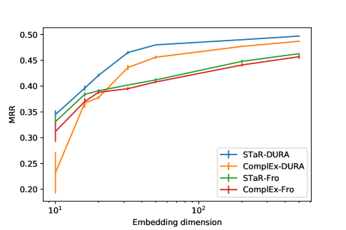
Figure 3: Comparison of STaR and ComplEx on WN18RR under different dimensions ($n\in\{10,16,20,32,50,200,500\}$) and regularization terms (Fro and DURA). Averages and standard deviations are computed over 5 runs for each case.

5.1 Further Comparison with ComplEx

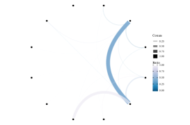
(a) WN18RR

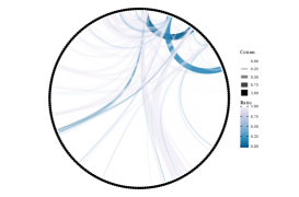
(b) FB15K237

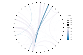
(c) YAGO3-10

Figure 4: The count and imbalance ratio of all possible pairs. An arc represents a pair. On the one hand, pair imbalance ratio $\psi$ is denoted by color, as blue means balance while gray means imbalance in contrast. On the other hand, the count is denoted by transparency and thickness, as thick and opaque means more while thin and transparent means less. It should be noticed that the thickness of the arcs is relative, so the arcs with the same thickness in different datasets may have different counts.

To show STaR outperforms ComplEx consistently, we conduct further experiments in different dimensions and regularization terms. As shown in Figure 3, STaR exceeds ComplEx on WN18RR persistently. Besides, both STaR and ComplEx improve by substituting DURA for Frobenius as the dimension increases. Additionally, STaR and ComplEx seem to intersect in an extremely high dimension, which leads us to further experiment in the following content.

Table 5: Link prediction results between STaR and ComplEx for extremely high-dimensional embedding (best for $n\in\{1000,2000,4000\}$). Better results are in bold.

	WN18RR		FB15K237		YAGO3-10
Model	MRR	Hits@10	MRR	Hits@10	MRR	Hits@10
ComlEx-DURA	0.490	0.573	0.371	0.561	0.583	0.710
STaR-DURA	0.499	0.585	0.370	0.558	0.584	0.713

As shown in the Tabel 5, STaR outperforms ComplEx on WN18RR prominently. However, these two are tied on FB15K237 and YAGO3-10 unexpectedly. We think such a phenomenon is due to the lack of non-commutativity patterns in them substantially. To verify our hypothesis, we further investigate those KGs from a new perspective.

5.2 Imbalance Ratio among KGs

In this part, we will verify the above hypothesis by introducing two matrices $\psi$ and $\Psi$ about the imbalance ratio.

We find that modeling commutativity and non-commutativity is useful only if both possible orders of a pair of relations appear in a KG. For instance, consider two relations $r_{1},r_{2}\in\mathcal{R}$, which have two possible orders of composition: $r_{1}\circ r_{2}$ and $r_{2}\circ r_{1}$. Therefore, if only one of them, e.g., $r_{1}\circ r_{2}$, exists in the KG, it is unnecessary to distinguish whether they are commutative or not, which we regard as an imbalance.

To this end, we propose two matrices $\psi$ and $\Psi$ to evaluate the imbalance ratio of pair and KG, respectively. For the details of these two matrices, please refer to Supplementary Material D.

Based on $\Psi$ of each benchmark as shown in Table 3, we observe that the imbalance is remarkable in FK15K237 and YAGO3-10. Moreover, we are aware that although some pairs have both orders, the counts between orders may have an enormous discrepancy. To show this more specifically, we visualize the pairs of three benchmark KGs. As shown in Figure 4, on the one hand, the majority of pairs are imbalanced in FB15K237 and YAGO3-10. On the other hand, although many imbalanced pairs exist in WN18RR, the balanced ones account for the majority as denoted by $\Psi$.

We believe the above analysis validates the hypothesis and explains the phenomenon. Furthermore, we think the discrepancy between KGs is rooted in the entities. Specifically, we notice that all entities are homogeneous in WordNet, which consists of words, while heterogeneous in Freebase and YAGO, built by various things like person, film, etc. Therefore, in KGs like WordNet, all relations connect things of the same kind. In contrast, in ones like Freebase and YAGO, most relations connect things of different kinds.

Therefore, for the relations in the imbalance KGs like FB15K237 and YAGO3-10, some pairs of them only have one meaningful order in the sense of semantics substantially. For instance, consider two relations: isDirectedBy and likeEating, whose combination makes sense in the order of $film\stackrel{{\scriptstyle\textit{IsDirectedBy}}}{{\longrightarrow}}human\stackrel{{\scriptstyle\textit{likeEating}}}{{\longrightarrow}}food$. However, when exchanging the order, we find that the tail entity of likeEating should be a kind of food, and the head entity of isDirectedBy should be a movie, which shows the inherent incompatibility in this order. More generally speaking, taking $\forall r_{1},r_{2}\in\mathcal{R}$ that has the order of combination $r_{1}\circ r_{2}$. Its other order $r_{2}\circ r_{1}$ is meaningless and nonexistent if the domain of head entity of $r_{1}$ and tail entity of $r_{2}$ are not intersected. In conclusion, we think that such a semantic character of these inter-kind relations explains the cause of the scarcity of non-commutativity in FB15K237 and YAGO3-10.

Table 6: Comparison of the MRR of STaR and ComplEx on WN18RR. $\bigtriangleup$ denotes improvement and $\bigtriangledown$ decreases on extremely high-dimensional settings.

Relation Name	Propotion	STaR	ComplEx	Improvement
hypernym	40.09%	0.193	0.175	$10.29\%\ \bigtriangleup$
derivationally related form	34.23%	0.956	0.959	$-0.31\%\ \bigtriangledown$
member meronym	8.52%	0.241	0.225	$7.11\%\ \bigtriangleup$
has part	5.55%	0.247	0.230	$7.39\%\ \bigtriangleup$
synset domain topic of	3.56%	0.409	0.387	$5.68\%\ \bigtriangleup$
instance hypernym	3.37%	0.420	0.409	$2.69\%\ \bigtriangleup$
also see	1.49%	0.634	0.631	$0.47\%\ \bigtriangleup$
verb group	1.30%	0.917	0.975	$-5.95\%\ \bigtriangledown$
member of domain region	1.06%	0.408	0.279	$46.24\%\ \bigtriangleup$
member of domain usage	0.73%	0.359	0.316	$13.61\%\ \bigtriangleup$
similar to	0.09%	1.000	1.000	$0.00\%\quad\,$

5.3 Improvements on WN18RR Come from Modeling Non-Commutativity Pattern

In FB15K237 and YAGO3-10, we have shown that imbalances are prevalent and thus explain why STaR and ComplEx are tied. Here we further experiment to corroborate that the improvement on WN18RR gains from modeling the non-commutativity pattern.

As shown in Table 6, STaR surpasses ComplEx in most relations. Although STaR slightly decreases in derivationally related form which is already high enough, it gains about $10\%$ in hypernym with the largest proportion. Correspondingly, we notice that in Figure 4(a) the outstanding thick blue arc denotes both $e_{1}\stackrel{{\scriptstyle hyp.}}{{\longrightarrow}}e_{2}\stackrel{{\scriptstyle\textit{d.r.f.}}}{{\longrightarrow}}e_{3}$ and $e_{1}\stackrel{{\scriptstyle\textit{d.f.r.}}}{{\longrightarrow}}e_{2}\stackrel{{\scriptstyle\textit{hyp.}}}{{\longrightarrow}}e_{3}$ are abundant in WN18RR. Besides, we find that these two relations are non-commutative. Therefore, we think such a correspondence validates that the improvement on WN18RR comes from modeling non-commutativity.

6 Conclusion

In this paper, we notice that none of the previous bilinear models can model all patterns and handle complex relations simultaneously. To fill the gap, we propose a bilinear model Scaling Translation and Rotation (STaR) consisting of these three basic modules. STaR solves both problems concurrently and achieves comparable results compared to previous baselines. Moreover, we also conduct a deep investigation to verify that our model is improved by handling relations or modeling patterns that previous bilinear models failed.

Supplementary Material

Appendix A Formal Definitions of 7 Relation Patterns

Consider triples of a completed KG $\mathcal{T}^{*}$, which contains all true facts for entities $\mathcal{E}$ and relations $\mathcal{R}$. Therefore, the former definition of those patterns are as follows:

1. Symmetry: For a relation $r\in\mathcal{R}$ and $\forall e_{1},e_{2}\in\mathcal{E}$, if $(e_{1},r,e_{2})\in\mathcal{T}^{*}$ then $(e_{2},r,e_{1})\in\mathcal{T}^{*}$.

2. Anti-Symmetry: For a relation $r\in\mathcal{R}$ and $\forall e_{1},e_{2}\in\mathcal{E}$, if $(e_{1},r,e_{2})\in\mathcal{T}^{*}$ then $(e_{2},r,e_{1})\notin\mathcal{T}^{*}$.

3. Composition: For relations $r_{1},r_{2},r_{3}\in\mathcal{R}$ and $\forall e_{1},e_{2},e_{3}\in\mathcal{E}$, if $(e_{1},r_{1},e_{2})\in\mathcal{T}^{*}\wedge(e_{2},r_{2},e_{3})\in\mathcal{T}^{*}$ then $(e_{1},r_{2},e_{3})\notin\mathcal{T}^{*}$. Therefor, $r_{3}$ is the composition of $r_{1}$ and $r_{2}$.

4. Commutativity: For relations $r_{1},r_{2}\in\mathcal{R}$ and $\forall e_{1},e_{2},e_{3}\in\mathcal{E}$, if $(e_{1},r_{1},e_{2})\in\mathcal{T}^{*}\wedge(e_{2},r_{2},e_{3})\in\mathcal{T}^{*}$ then $(e_{1},r_{2},e_{2})\in\mathcal{T}^{*}\wedge(e_{2},r_{1},e_{3})\in\mathcal{T}^{*}$.

5. Non-Commutativity: For relations $r_{1},r_{2}\in\mathcal{R}$ and $\forall e_{1},e_{2},e_{3}\in\mathcal{E}$, if $(e_{1},r_{1},e_{2})\in\mathcal{T}^{*}\wedge(e_{2},r_{2},e_{3})\in\mathcal{T}^{*}$ then $(e_{1},r_{2},e_{2})\notin\mathcal{T}^{*}\vee(e_{2},r_{1},e_{3})\notin\mathcal{T}^{*}$.

6. Inversion: For relations $r_{1},r_{2}\in\mathcal{R}$ and $\forall e_{1},e_{2}\in\mathcal{E}$ if $(e_{1},r_{1},e_{2})\in\mathcal{T}^{*}$ and $(e_{2},r_{2},e_{1})\in\mathcal{T}^{*}$ iff $e_{2}=e_{1}$.

Appendix B Proof of Proposition 1

Proof.

Since each relationship is represented by a matrix $R_{*}$ and the matrix multiplication stands composition operator $\circ$, here we will show how to model all 6 properties by taking some cases of $R_{*}$ and how to handle complex relations by considering a fixed margin $\gamma$ .

1. Symmetry: Here we take $r^{c}_{i}=0,\quad i=1,3,\cdots,n-1$ and $\tau=\mathbf{0}$. Then STaR degenerates to DistMult. Thus $\hat{h}^{T}R_{*}\hat{t}=\hat{t}^{T}R_{*}\hat{h}$ and STaR models the symmetry pattern.

2. Anti-Symmetry: Here we take $r^{c}=\mathbf{0}$ and $\tau\in\mathbb{R}^{n\times 1}$, and STaR degenerates to TransE(Bordes et al. 2013). Then it models the anti-symmetry pattern, since if $\|h+r-t\|=0$ then $\|t+r-h\|\neq 0$ for $h,r,t\neq\mathbf{0}$.

3. Composition: It is equivalent that taking $R_{*}^{1},R_{*}^{2}$ then $R_{*}^{1}\cdot R_{*}^{2}$ is still in the form of $R_{*}$:

   $$R_{*}^{1}\cdot R_{*}^{2} =\begin{bmatrix}R_{c}^{1}\\ (\tau^{1})^{T}&1\end{bmatrix}\cdot\begin{bmatrix}R_{c}^{2}\\ (\tau^{2})^{T}&1\end{bmatrix}$$

   $$=\begin{bmatrix}R_{c}^{1}\cdot R_{c}^{2}\\ (\tau^{1})^{T}R_{c}^{2}+(\tau^{2})^{T}&1\end{bmatrix},$$

   thus STaR can model the composition pattern.

4. Commutativity: If we take $\tau=\mathbf{0}$, then STaR degenerates to ComplEx matrix, which is a block diagonal matrix and can be exchanged $R_{*}^{1}\cdot R_{*}^{2}=R_{*}^{2}\cdot R_{*}^{1}$. Thus STaR can model the commutativity pattern.

5. Non-Commutativity: As demonstrated in Figure 1(b) and Figure 1(c), the translation and rotation are non-commutative. Then, we take $\tau^{1}=\mathbf{0}$ and $r_{i}^{2}+r_{i+1}^{2}=1,\quad i=1,3,\cdots,n-1$ to degenerate $R_{*}^{1}$ into a pure rotation matrix, and $r_{c}^{2}=\mathbf{0}$ to degenerate $R_{*}^{2}$ into a pure translation matrix. Then, $R_{*}^{1}\cdot R_{*}^{2}\neq R_{*}^{2}\cdot R_{*}^{1}$

6. Inversion: Here we take $\tau=\mathbf{0}$, then for a $R_{*}^{1}$, there exists $R_{*}^{2}$ that has $(R_{*}^{1})^{T}=R_{*}^{2}$. Therefore, we have $\hat{h}^{T}R_{*}^{1}\hat{t}=\hat{t}^{T}R_{*}^{2}\hat{h}$.

7. Complex relations Here we follow (Chao et al. 2021) and treat the ability of model handling complex relations is adaptive adjusting the margin given a fixed one. Specifically, we set this fixed margin as $\gamma$, and a candidate is true means the score of the corresponding triple $s(h,r,t)$ is greater than $\gamma$:

   $$\gamma<h^{T}Rt.$$ (9)

   If a constant $\alpha$ is multiplied on both side and only changes $R$, then we say it adaptively adjusts the margin. Therefore, for a $(h,r,t)$, STaR has:

   $$\gamma<\hat{h}^{T}R_{*}\hat{t}$$ (10)

   $$\alpha \gamma<\alpha\hat{h}^{T}R_{*}\hat{t}$$

   $$\alpha \gamma<\hat{h}^{T}\alpha\begin{bmatrix}R_{c}&\\ &1\end{bmatrix}\begin{bmatrix}I\\ \tau^{T}&1\end{bmatrix}\hat{t}$$

   $$\alpha \gamma<\hat{h}^{T}\left(\begin{bmatrix}\alpha R_{c}&\\ &1\end{bmatrix}+\begin{bmatrix}\mathbf{0}^{n\times n}&\\ &(\alpha-1)\end{bmatrix}\right)\begin{bmatrix}I\\ \tau^{T}&1\end{bmatrix}\hat{t}$$

   $$\alpha \gamma<\hat{h}^{T}\begin{bmatrix}\alpha R_{c}&\\ &1\end{bmatrix}\begin{bmatrix}I\\ \tau^{T}&1\end{bmatrix}\hat{t}+(\alpha-1)$$

   $$\alpha (\gamma-1)+1<\hat{h}^{T}R_{*}^{\prime}t,$$

   since $R_{*}$ and $\alpha$ are learnable, the margin can be dynamic adjust without changing $h$ and $t$. Thus, we could say that STaR can handle complex relations.

Based on the discussion above, we could conclude that STaR is capable to model all 6 patterns and handle complex relations. ∎

Appendix C Details of DURA

For a bilinear model $h^{T}Rt$ in real value, the DURA regularization is:

$$\|h\|^{2}_{2}+\|Rt\|_{2}^{2}+\|t\|_{2}^{2}+\|h^{T}R\|_{2}^{2}.$$ (11)

Then, for STaR, we have:

$$\|h\|^{2}_{2}+\|Rt\|_{2}^{2}+\|t\|_{2}^{2}+\|h^{T}R\|_{2}^{2}$$ (12)

$$= \|\hat{h}\|^{2}_{2}+\|R_{*}\hat{t}\|_{2}^{2}+\|\hat{t}\|_{2}^{2}+\|\hat{h}^{T}R_{*}\|_{2}^{2}$$

$$= \|h\|^{2}_{2}+\|t\|^{2}_{2}+\|h^{T}R_{c}+\tau\|^{2}_{2}+\|R_{c}t\|^{2}_{2}+\tau^{T}t+4.$$

The emergence of constant $4$, which can be ignored in the optimization, is because we use $\hat{h},\hat{t}$ having an extra dimension with constant 1.

Appendix D Details of $\psi$ and $\Psi$

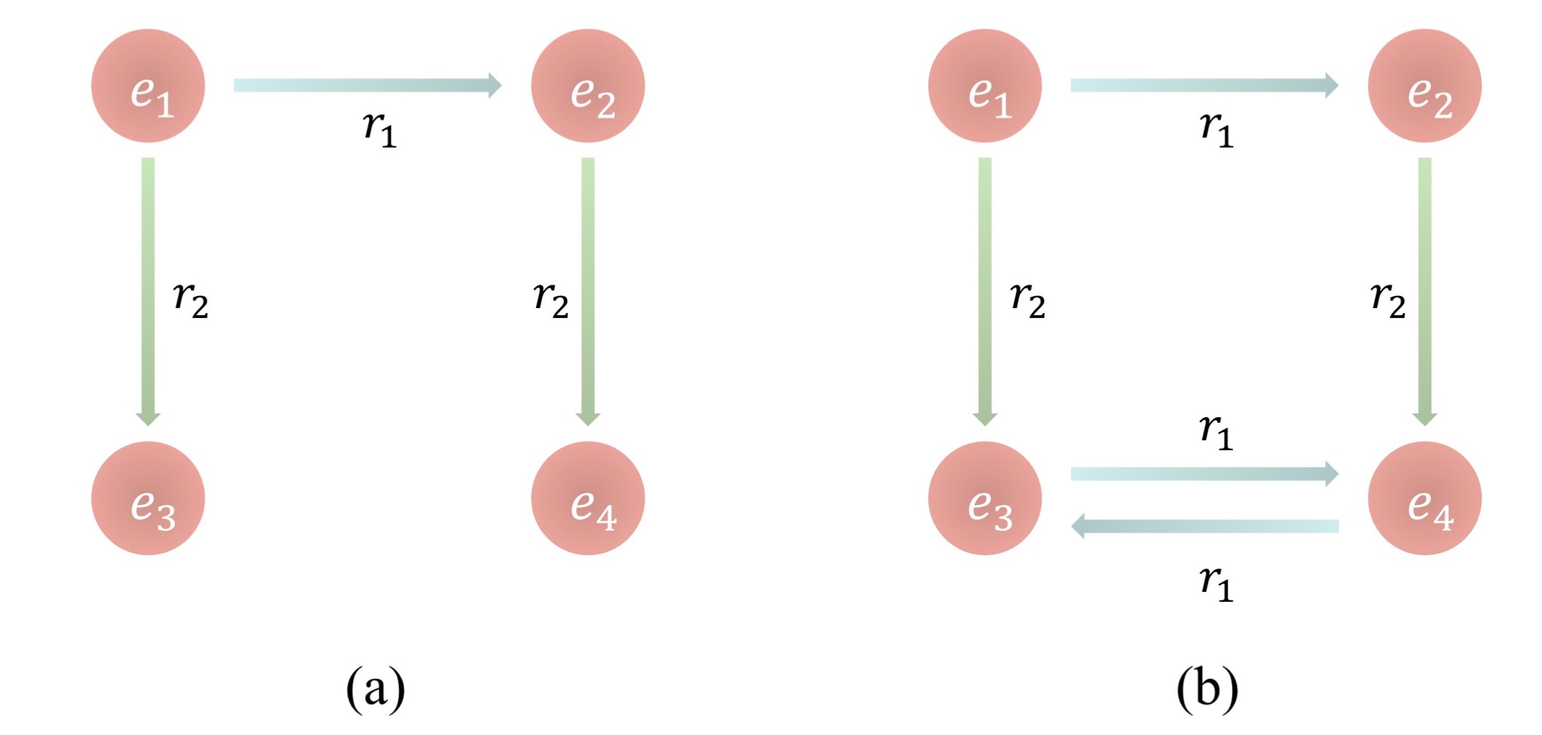
Figure 5: Toy examples demonstrate how to count $\#\text{triple}_{ij}$

For each possible relation pair $(r_{i},r_{j})\in(\mathcal{R},\mathcal{R})$, we count its corresponding triple in the training set $\mathcal{T}_{train}$ as $\#\text{triple}_{ij}$ and $\#\text{triple}_{ji}$. For Instance, in the Figure 5, $\#\text{triple}_{12}=1$ and $\#\text{triple}_{21}=0$ in the left hand example while $\#\text{triple}_{12}=1$ and $\#\text{triple}_{21}=2$ in the right one. Then, we define the imbalance ratio of a relation pair $\psi_{ij}$ as:

$$\psi_{ij}=2\cdot\frac{\max{\{\#\text{triple}_{ij},\#\text{triple}_{ji}\}}}{\#\text{triple}_{ij}+\#\text{triple}_{ji}}-1.$$ (13)

Meanwhile, we treat a pair as both if $\#\text{triple}_{ij}>0$ and $\#\text{triple}_{ji}>0$, and single if only one of them greater than $0$. Based on that, we count the triples of both and single as $\#\text{triple}_{both}$ and $\#\text{triple}_{single}$ respectively. Thus, we define a similar matrix $\Psi$ for the imbalance ratio of train set:

$$\Psi=\frac{\#\text{triple}_{single}}{\#\text{triple}_{both}+\#\text{triple}_{single}}.$$ (14)

References

- An et al. (2018) An, B.; Chen, B.; Han, X.; and Sun, L. 2018. Accurate Text-Enhanced Knowledge Graph Representation Learning. In NAACL-HLT, 745–755.
- Balazevic, Allen, and Hospedales (2019a) Balazevic, I.; Allen, C.; and Hospedales, T. M. 2019a. Multi-relational Poincaré Graph Embeddings. In NeurIPS, 4465–4475.
- Balazevic, Allen, and Hospedales (2019b) Balazevic, I.; Allen, C.; and Hospedales, T. M. 2019b. TuckER: Tensor Factorization for Knowledge Graph Completion. In EMNLP/IJCNLP (1), 5184–5193.
- Bordes et al. (2013) Bordes, A.; Usunier, N.; García-Durán, A.; Weston, J.; and Yakhnenko, O. 2013. Translating Embeddings for Modeling Multi-relational Data. In NeurIPS, 2787–2795.
- Chami et al. (2020) Chami, I.; Wolf, A.; Juan, D.; Sala, F.; Ravi, S.; and Ré, C. 2020. Low-Dimensional Hyperbolic Knowledge Graph Embeddings. In ACL, 6901–6914.
- Chao et al. (2021) Chao, L.; He, J.; Wang, T.; and Chu, W. 2021. PairRE: Knowledge Graph Embeddings via Paired Relation Vectors. In Zong, C.; Xia, F.; Li, W.; and Navigli, R., eds., ACL/IJCNLP(1), 4360–4369.
- Dettmers et al. (2018) Dettmers, T.; Minervini, P.; Stenetorp, P.; and Riedel, S. 2018. Convolutional 2D Knowledge Graph Embeddings. In AAAI, 1811–1818.
- Ji et al. (2021) Ji, S.; Pan, S.; Cambria, E.; Marttinen, P.; and Yu, P. S. 2021. A Survey on Knowledge Graphs: Representation, Acquisition, and Applications. IEEE Trans Neural Netw Learn Syst., 1–21.
- Lacroix, Usunier, and Obozinski (2018) Lacroix, T.; Usunier, N.; and Obozinski, G. 2018. Canonical Tensor Decomposition for Knowledge Base Completion. In ICML, volume 80, 2869–2878.
- Lin et al. (2015) Lin, Y.; Liu, Z.; Sun, M.; Liu, Y.; and Zhu, X. 2015. Learning Entity and Relation Embeddings for Knowledge Graph Completion. In AAAI, 2181–2187.
- Liu, Wu, and Yang (2017) Liu, H.; Wu, Y.; and Yang, Y. 2017. Analogical Inference for Multi-relational Embeddings. In ICML, volume 70, 2168–2178.
- Mahdisoltani, Biega, and Suchanek (2015) Mahdisoltani, F.; Biega, J.; and Suchanek, F. M. 2015. YAGO3: A Knowledge Base from Multilingual Wikipedias. In CIDR.
- Mikolov et al. (2013) Mikolov, T.; Sutskever, I.; Chen, K.; Corrado, G. S.; and Dean, J. 2013. Distributed Representations of Words and Phrases and their Compositionality. In NeurIPS, 3111–3119.
- Mohammed, Shi, and Lin (2018) Mohammed, S.; Shi, P.; and Lin, J. 2018. Strong Baselines for Simple Question Answering over Knowledge Graphs with and without Neural Networks. In NAACL-HLT (2), 291–296.
- Nguyen et al. (2018) Nguyen, D. Q.; Nguyen, T. D.; Nguyen, D. Q.; and Phung, D. Q. 2018. A Novel Embedding Model for Knowledge Base Completion Based on Convolutional Neural Network. In NAACL-HLT (2), 327–333.
- Nickel, Rosasco, and Poggio (2016) Nickel, M.; Rosasco, L.; and Poggio, T. A. 2016. Holographic Embeddings of Knowledge Graphs. In AAAI, 1955–1961.
- Nickel, Tresp, and Kriegel (2011) Nickel, M.; Tresp, V.; and Kriegel, H. 2011. A Three-Way Model for Collective Learning on Multi-Relational Data. In ICML, 809–816.
- Paul (1981) Paul, R. P. 1981. Robot manipulators: mathematics, programming, and control: the computer control of robot manipulators. Richard Paul.
- Schlichtkrull et al. (2018) Schlichtkrull, M. S.; Kipf, T. N.; Bloem, P.; van den Berg, R.; Titov, I.; and Welling, M. 2018. Modeling Relational Data with Graph Convolutional Networks. In ESWC, volume 10843, 593–607.
- Sun et al. (2019) Sun, Z.; Deng, Z.; Nie, J.; and Tang, J. 2019. RotatE: Knowledge Graph Embedding by Relational Rotation in Complex Space. In ICLR.
- Toutanova and Chen (2015) Toutanova, K.; and Chen, D. 2015. Observed versus latent features for knowledge base and text inference. In Proceedings of the 3rd Workshop on Continuous Vector Space Models and their Compositionality, 57–66. Beijing, China.
- Trouillon et al. (2016) Trouillon, T.; Welbl, J.; Riedel, S.; Gaussier, É.; and Bouchard, G. 2016. Complex Embeddings for Simple Link Prediction. In ICML, volume 48, 2071–2080.
- Wang et al. (2017) Wang, J.; Wang, Z.; Zhang, D.; and Yan, J. 2017. Combining Knowledge with Deep Convolutional Neural Networks for Short Text Classification. In IJCAI, 2915–2921.
- Wang et al. (2014) Wang, Z.; Zhang, J.; Feng, J.; and Chen, Z. 2014. Knowledge Graph Embedding by Translating on Hyperplanes. In AAAI, 1112–1119.
- Xu and Li (2019) Xu, C.; and Li, R. 2019. Relation Embedding with Dihedral Group in Knowledge Graph. In ACL (1), 263–272.
- Yang et al. (2015) Yang, B.; Yih, W.; He, X.; Gao, J.; and Deng, L. 2015. Embedding Entities and Relations for Learning and Inference in Knowledge Bases. In ICLR.
- Yang, Sha, and Hong (2020) Yang, T.; Sha, L.; and Hong, P. 2020. NagE: Non-Abelian Group Embedding for Knowledge Graphs. In CIKM, 1735–1742.
- Yao, Mao, and Luo (2019) Yao, L.; Mao, C.; and Luo, Y. 2019. KG-BERT: BERT for Knowledge Graph Completion. arXiv:1909.03193.
- Zhang et al. (2016) Zhang, F.; Yuan, N. J.; Lian, D.; Xie, X.; and Ma, W. 2016. Collaborative Knowledge Base Embedding for Recommender Systems. In KDD, 353–362.
- Zhang et al. (2019) Zhang, S.; Tay, Y.; Yao, L.; and Liu, Q. 2019. Quaternion Knowledge Graph Embeddings. In NeurIPS, 2731–2741.
- Zhang, Cai, and Wang (2020) Zhang, Z.; Cai, J.; and Wang, J. 2020. Duality-Induced Regularizer for Tensor Factorization Based Knowledge Graph Completion. In NeurIPS.
- Zhang et al. (2020a) Zhang, Z.; Cai, J.; Zhang, Y.; and Wang, J. 2020a. Learning Hierarchy-Aware Knowledge Graph Embeddings for Link Prediction. In AAAI, 3065–3072.
- Zhang et al. (2020b) Zhang, Z.; Zhuang, F.; Zhu, H.; Shi, Z.; Xiong, H.; and He, Q. 2020b. Relational Graph Neural Network with Hierarchical Attention for Knowledge Graph Completion. In AAAI, 9612–9619.