Gigahertz Sub-Landauer Momentum Computing

Abstract

We introduce a fast and highly-efficient physically-realizable bit swap. Employing readily available and scalable Josephson junction microtechnology, the design implements the recently introduced paradigm of momentum computing. Its nanosecond speeds and sub-Landauer thermodynamic efficiency arise from dynamically storing memory in momentum degrees of freedom. As such, during the swap, the microstate distribution is never near equilibrium and the memory-state dynamics fall far outside of stochastic thermodynamics that assumes detailed-balanced Markovian dynamics. The device implements a bit-swap operation—a fundamental operation necessary to build reversible universal computing. Extensive, physically-calibrated simulations demonstrate that device performance is robust and that momentum computing can support thermodynamically-efficient, high-speed, large-scale general-purpose computing that circumvents Landauer’s bound.

I Introduction

Ever since the first exorcism of Maxwell’s demon [1], determining how much energetic input a particular computation requires has been a broadly-appreciated theoretical question. In the current century, however, the question has taken on a markedly practical bent; a familiar example is the evolution of Moore’s Law from initially provocative speculations decades ago to now addressing material, thermodynamic, and fabrication restrictions [2, 3, 4, 5, 6]. Transistor-based microprocessing presents fundamental scaling challenges that strictly limit potential directions for future optimization, and these challenges are no longer speculative. Clock speed, to take one example, has been essentially capped for two decades due to energy dissipation at high rates [7, 8]. By some measures, Moore’s law is already dead—as integrated circuit manufacturers go vertical, rather than face the expense of creating smaller transistors for 2D circuits that yield only marginal gains [9, 10, 11].

Given predicted explosive growth in societal demands for information processing and that digital microelectronics is now approaching the physical limits of available architectures [12], exploring alternative computing paradigms is not only prudent but necessary. One alluring vision for the future involves hybrid devices, composed of a suite of computing modules—classical/quantum, digital/analog, deterministic/thermal—each with its own architecture and function that operate in concert. A hybrid architecture allows dynamically harnessing the processing node best suited for the task at hand. The underlying insight is that a computing device’s physical substrate should match its desired processing function [13]. In keeping with this, momentum computing demonstrated that low dissipation operations do not require quasi-static operation [14]. That is, energy-efficient computation can be fast in a low-dissipation device.

Reference [14] introduced a design framework and theory for an arbitrarily low-cost, high-speed bit swap, a logically-reversible gate (the only known logical framework with no nontrivial lower bound on its dissipation [12, 15, 16].) It demonstrated that a universal reversible gate—a Fredkin gate [17, 18]—can be built by coupling three such devices together. However, any particular physically-instantiated implementation will come with its own restrictions and considerations that are likely to disallow performing the swap exactly as theorized. And so, an implementation linked to a particular substrate must be built and analyzed in its own right.

We present a physically-realizable device and control protocols that implement a bit swap gate that operates in the sub-$k_{\text{B}}T$ energy regime using superconducting Josephson junctions (JJs)—a well-known and scalable microtechnology. We recently used this device to measure the thermodynamic performance of bit erasure [19, 20]. That extensive experimental effort demonstrated in practical terms that the device proposed here is realizable with today’s microfabrication technologies and allows for detailed studies of thermodynamic costs. And so, the device’s design and control protocol open up exploring the energy scales of highly energy-efficient, high-speed, general-purpose computing.

The Landauer

While there are many different quantities one might wish to optimize, the perspective here sets the goal as minimizing the net work invested $W$ when performing logical operations. It is well known that the most pressing physical limits on modern computation are power constraints [21], thus the measure is well suited to diagnose the problems with current devices as well as potential strengths of new ones.

For over half a century now Landauer’s Principle has exerted a major impact on the contemporary approach to thermodynamic costs of information processing [22, 23]. Its lower bound of $k_{\text{B}}T\ln 2$ energy dissipated per bit erased has served as standard candle for energy use in physical information processing. To aid comparing other computing paradigms and protocols, we refer to this temperature-dependent information-processing energy scale as a Landauer: approximately a few zeptojoules at room temperature, and a few hundredths of a zeptojoule at liquid He temperatures. See Appendix A for further comparisons.

To appreciate the potential benefits of momentum computing operating at sub-Landauer energies we ask where contemporary computing is on the energy scale. Consider recent stochastic thermodynamic analyses of single-electron transistor logic gates [24, 25]—analogs to conventional CMOS technology. The upshot is that these technologies currently operate between $10^{3}$ and $10^{4}$ Landauers. More to the point, devices using CMOS-based technology will only ever be able to operate accurately above $\approx 10^{2}$ Landauers [15, 12]. In short, momentum computing promises substantial improvements in efficiency with no compromise in speed.

Outline

Here we provide a brief overview of each section and appendix in the text. Section II explains the importance of bit-swap operations and summarizes the protocol presented in Ref. [14]. Section III introduces the physical substrate, highlights why it is a good candidate, and addresses design restrictions. Section IV reports quantitative results on device performance as measured through detailed simulations of the microscopic degrees of freedom. Section V compares them to related results, both contemporary and foundational. Section VI concludes, summarizing the results and briefly outlining future directions and challenges for scaling up to general-purpose computing.

Appendices include details necessary to understand the process by which the parameter space of control protocols was restricted and local work minima were found in simulation. Additionally, they also provide expository information that the interested reader might find relevant. In particular, Appendix A discusses the temperature dependent energy scale, the “Landauer”. Appendix B outlines key physical differences between continuous-time Markov chains and hidden Markov chains. Appendix C presents the equations of motion of the bit-swap Josephson junction circuit in their dimensional form and their transformation to simulation-appropriate dimensionless equations. Appendix D details the process of algebraically eliminating large swaths of protocol parameter space. And, finally, Appendix E discusses the algorithmic details of the simulations.

II Bit Swap

The Landauer cost stood as a reference for so long since bit erasure is the dominant source of unavoidable dissipation when implementing universal computing with transistor logic gates. It is the elementary binary computation that most changes the Shannon entropy of the distribution over memory states. In this way, one sees $k_{\text{B}}T\ln 2$ not just as the cost of erasure, but as the cost of the maximally dissipative elementary operation on which conventional computing relies. And so, the Landauer naturally sets the energy scale for conventional computing.

Taking inspiration from Landauer’s pioneering work, we investigate the cost of the most expensive operation necessary to physically implement universal momentum computing: a bit swap. The ideal bit swap has no error, but in the thermodynamic setting one is also interested in an implementation’s fidelity. And so, we write a swap with error rates $\epsilon_{0}$ and $\epsilon_{1}$ as a stochastic mapping between memory states $m\in\{0,1\}$ from time $0$ to time $\tau$:

$$P_{\epsilon}(m_{\tau}|m_{0})=\left[\begin{array}[]{cc}\epsilon_{0}&1-\epsilon_{0}\\ 1-\epsilon_{1}&\epsilon_{1}\end{array}\right]~{}.$$

The bit swap’s dominance in the cost of universal momentum computing can be appreciated by considering the input-output mapping of the Fredkin gate—a $3$-bit universal gate with memory states $m_{x}m_{y}m_{z}$, $m_{i}\in\{0,1\}$. All inputs are preserved except for the exchange $101\leftrightarrow 110$. We can decompose the informational state space into two regions. If $m_{x}=0$, the operation is simply an identity, which trivially is costless. If $m_{x}=1$ and $m_{y}=m_{z}$, we once again have an identity. Thus, it is only the subspace of $m_{x}=1$, where $m_{y}\neq m_{z}$ that a swap must take place. Reference [14] provides explicit potentials that impose effectively 1D swap potentials on a full 3-bit state space in order to implement the Fredkin gate, demonstrating that only 1D swap operations need contribute to the operation’s thermodynamic cost.

II.1 Momentum Computing Realization

Storing information in a one-dimensional state space, it is not clear how to operate a thermodynamically-efficient bit swap with high accuracy. (In this, we recall the conventional interpretation of efficient to mean quasistatic or constantly-thermalizing Markovian dynamics [26, 27].) At time $t$ in the operation, the distribution of initial conditions corresponding to $m(t=0)=0$ must overlap with that corresponding to $m(t=0)=1$. And, from that point forward it is impossible to selectively separate them based on their initial positions. Information, and so reversibility, is lost.

Consider, instead, a computation that happens faster than the equilibration timescale of the physical substrate and its thermal environment. In this regime, a particle’s instantaneous momentum can be commandeered to carry useful information about its future behavior. Our protocol operates on this timescale, using the full phase space of the underlying system’s degrees of freedom to transiently store information in their momenta. Due to this, the instantaneous microstate distribution is necessarily far from equilibrium during the computation. Moreover, the coarse-grained memory-state dynamics during the swap are not Markovian; despite both the net transformation over the memory states and the microscopic phase space dynamics being Markovian. Nonetheless, the system operates orders of magnitude more efficiently than current CMOS but, competing with CMOS, the dynamics evolve nonadiabatically in finite time—on nanosecond timescales for our physical implementation below.

In this way, momentum computing offers up device designs and protocols that accomplish information processing that is at once fast, efficient, and low error. There is a trade-off—a loss of Markovianity in the memory-state dynamics. That noted, the dynamics of the memory states are faithfully described by continuous-time hidden Markov chains (CTHMCs) [28, 29, 30], rather than the continuous-time Markov chains (CTMCs) that are common in stochastic thermodynamics [26, 27]. See Appendix. B for a brief review.

II.2 Idealized Protocol

Reference [14] describes a perfectly-efficient protocol for implementing a swap in finite time. The operation is straightforward. We begin with an ensemble of particles subject to a storage potential. The potential energy landscape $V^{\text{\text{store}}}(x)$ must contain at least two potential minima—positioned, say, at $x=\pm x_{0}$—with an associated energy barrier equal to $\text{max}\{V^{\text{store}}(x),x\in(-x_{0},x_{0})\}-V^{\text{store}}(x_{0})$. During storage, a particle’s environment is a thermal bath at temperature $T$. As the height of the potential energy barrier rises relative to the bath energy scale $k_{\text{B}}T$, the probability that the particle transitions between left ($x<0$) and right ($x\geq 0$) decreases exponentially. In this way, if we assign the left half of the position space to memory state $0$ and the right half to memory state $1$, the energy landscape is capable of metastably storing a bit $m\in\{0,1\}$.

At the protocol’s beginning, we instantaneously apply a new potential energy landscape $V^{\text{comp}}\equiv kx^{2}/2$. The system is then temporarily isolated from its thermal environment, resulting in the particles undergoing a simple harmonic oscillation. Waiting a time $\tau$ until the oscillation is only half completed, the potential is returned to $V^{\text{store}}$. The initial conditions—for which $x_{0}<0$ $(x_{0}>0)$—have then been mapped to $x_{\tau}>0$ $(x_{\tau}<0)$, achieving the desired swap computation. If $V^{\text{store}}$ is an even function of $x$, the computation requires zero invested work as well. This follows since the harmonic motion created a mirror image to the original distribution and the energy imparted to the system at $t=0$ is completely offset by the energy extracted from the system turning off $V^{\text{comp}}$ at $t=\tau$.

III Physical Instantiation

Due to its conceptual simplicity the protocol does not require any particular physical substrate. That said, the practical feasibility of performing such a computation must be addressed. One obvious point of practical concern is assuming the system can be isolated from its thermal environment during the computation. However, total isolation is not necessary. If $\tau\ll\tau_{R}$—the relaxation timescale associated with the energy flux rate between the system and its thermal bath—then the device performs close to the ideal case of zero coupling.

As proof of concept, Ref. [14]’s simulations showed that this class of protocol is robust: thermodynamic performance persists in the presence of imperfect isolation from the thermal environment, albeit at an energetic cost. Thus, a system that obeys significantly-underdamped Langevin dynamics is an ideal candidate as the physical substrate for bit swap.

We analyze in detail one physical instantiation—a gradiometric flux logic cell (Fig. 1), a mature technology for information processing. With suitable scale definitions, the effective degrees of freedom—Josephson phase sum $\varphi$ and difference $\varphi_{\text{dc}}$—follow a dimensionless Langevin equation [31, 32, 33, 34, 19, 20]:

$$dv^{\prime}=-\lambda v^{\prime}dt^{\prime}-\theta\partial_{x^{\prime}}U^{\prime}+\eta r(t)\sqrt{2dt^{\prime}}~{},$$ (1)

where $x^{\prime}\equiv(\varphi,\varphi_{\text{dc}})$ and $v^{\prime}\equiv(\dot{\varphi},\dot{\varphi_{\text{dc}}})$ are vector representations of the dynamical coordinates. Enacting a control protocol on this system involves changing the parameters of the potential over time:

$$U^{\prime}(t^{\prime}) =U/U_{0}$$ (2)

$$=(\varphi-\varphi_{x}(t^{\prime}))^{2}/2+\gamma(\varphi_{\text{dc}}-\varphi_{\text{xdc}}(t^{\prime}))^{2}/2$$

$$\qquad+\beta\cos\varphi\cos(\varphi_{\text{dc}}/2)-\delta\beta\sin\varphi\sin(\varphi_{\text{dc}}/2)~{}.$$

Figure 1: Gradiometric flux logic cell: The superconducting current has two important flow modes. One circulation around the inner loop—a DC SQUID. And, the other, a flow through the Josephson junctions in the inner loop and around the outer conductor pickup loops—an AC SQUID [32]. This is the origin of the variable subscripts to distinguish $\varphi$ from $\varphi_{\text{dc}}$ and $\varphi_{x}$ from $\varphi_{\text{xdc}}$.

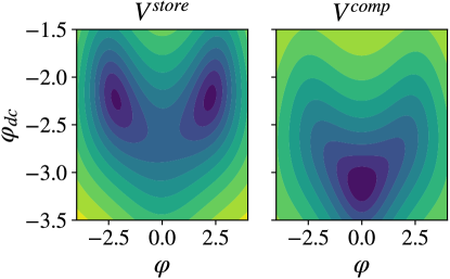
Figure 2: (Left) $V^{\text{store}}$, the bistable storage potential. (Right) $V^{\text{comp}}$, the “banana-harmonic” potential. These potential energy profiles serve as qualitative pictures to represent prototypical computational and storage potentials, and do not represent any particularly favorable parameter set.

The relationships between the circuit parameters and the parameters in the effective potential $U^{\prime}$ are as follows. $\varphi=(\varphi_{1}+\varphi_{2})/2-\pi$ and $\varphi_{\text{dc}}=(\varphi_{2}-\varphi_{1})$, where $\varphi_{1}$ and $\varphi_{2}$ are the phases across the two Josephson elements; $\varphi_{x}=2\pi\phi_{x}/\Phi_{0}-\pi$ and $\varphi_{\text{xdc}}=2\pi\phi_{xdc}/\Phi_{0}$, where $\Phi_{0}$ is the magnetic flux quantum and $(\phi_{x},\phi_{xdc})$ are external magnetic fluxes applied to the circuit; $U_{0}=\left(\Phi_{0}/2\pi\right)^{2}/L$, $\gamma=L/2\ell$, $\beta=I_{+}2\pi L/\Phi_{0}$, and $\delta\beta=I_{-}2\pi L/\Phi_{0}$, where $L$ and $2\ell$ are geometric inductances; and $I_{\pm}\equiv I_{c1}\pm I_{c2}$ are the sum and difference of the critical currents of the two Josephson junctions. All parameters are real and it is assumed that $\gamma>\beta>1\gg\delta\beta$.

Some particularly important parameters of $U^{\prime}$ are $\varphi_{x}$ and $\varphi_{\text{xdc}}$, which control the potential’s shape by where the the dynamical variables $\varphi$ and $\varphi_{\text{dc}}$ localize in equilibrium, and $\gamma$, which controls how quickly $\varphi_{\text{dc}}$ localizes to the bottom of the quadratic well centered near $\varphi_{\text{dc}}=\varphi_{\text{xdc}}$. At certain control parameters ($\varphi_{x},\varphi_{\text{xdc}}$), the effective potential contains only two minima: one located at $\varphi<0$ and one at $\varphi>0$. So, the device is capable of metastably storing a bit, as described above. In point of fact, the logic cell has been often used as a double well in $\varphi$ with a controllable tilt and barrier height [32, 34, 19].

The Langevin equation’s coupling constants, $\lambda$ and $\eta$, determine the rate of energy flow between the system and its thermal environment and the. They depend on the parameters $L$, $R$, and $C$. In the regimes at which one typically finds $L$, $C$, and $R$ and with temperatures around $1$ K, the system is very underdamped; ring-down times are $\mathcal{O}(10^{3})$ oscillations about the local minima. (Notably, the device thermalizes at a rate proportional to $R^{-1}$. A tunable $R$ allows the device to transition from the underdamped to overdamped regime, allowing for rapid thermalization, if desired.) Finally, $\theta$ is a dimensionless factor that depends on the relative inertia of the two degrees of freedom, it depends on the circuit architecture. Appendix C gives the equations of motion and thorough definitions of all parameters and variables in terms of dimensional quantities.

III.1 Realistic Protocol

With the device’s physical substrate set, we now show how to design energy-efficient bit-swap control protocols. There are four parameters that depend primarily on device fabrication: $I_{c1}$, $I_{c2}$, $R$, and $C$. Two that depend on the circuit design: $L$ and $\ell$. And, four that allow external control: $\varphi_{x}$, $\varphi_{\text{xdc}}$, $T$ (the environmental temperature), and $\tau$ (the computation time). Without additional circuit complexities to allow tunable $L$, $R$, and $C$, we assume that once a device is made, any given protocol can only manipulate $\varphi_{x}$, $\varphi_{\text{xdc}}$, $T$, and $\tau$. A central assumption is that computation happens on a timescale over which the thermal environment has minimal effect on the dynamics, so the primary controls are $\varphi_{x}$, $\varphi_{\text{xdc}}$, and $\tau$. $\varphi_{x}$ is associated with asymmetry in the informational subspace, and will only take a nonzero value to help offset asymmetry from the $\delta\beta$ term in $U^{\prime}$. Thus, $\varphi_{\text{xdc}}$ primarily controls the difference between $V^{\text{comp}}$ and $V^{\text{store}}$, while $\tau$ governs how long we subject the system to $V^{\text{comp}}$.

$V^{\text{store}}$ must be chosen to operate the device in a parameter regime admitting two minima on either side of $\varphi=0$ as in Fig. 2. They must also be sufficiently separated so that they are distinct memory states when immersed in an environment of temperature $T$.

In the ideal case, $V^{\text{comp}}$ is a quadratic well with an oscillation period $\tau=\pi\sqrt{m/k}$. However, $U$ will never give an exact quadratic well unless $\beta=\delta\beta=0$. So, a suitable replacement is necessary. The closest approximate is at the relatively obvious choice $\varphi_{\text{xdc}}=-2\pi$. In this case, the minima of both the quadratic and the periodic part of the potential lie on top of each other and the potential is well approximated by a quadratic function over most of the relevant position-domain.

However, due to restrictions on $V^{\text{store}}$, transitioning between $V^{\text{store}}$ and $V^{\text{comp}}$ may induce unnecessarily large dissipation since the oscillations in the $\varphi_{\text{dc}}$ dimension have a large amplitude. (See Appendix D for details.) Instead, to dissipate the minimum energy, the control parameters must balance placing the system as close as possible to the pitchfork bifurcation where the two wells merge, while still maintaining dynamics that induce the $\varphi<0$ and $\varphi>0$ informational states to swap places due to an approximately harmonic oscillation. Near this parameter value, one typically finds a “banana-harmonic” potential energy landscape. (See Fig. 2 for a comparison of the distinct potential profiles for storage and computation.)

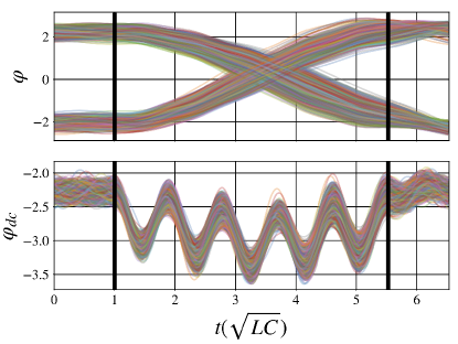
Figure 3: A dynamic computation: $1,500$ trajectories from $V^{\text{store}}$’s equilibrium distribution in the $\varphi$ (top) and $\varphi_{\text{dc}}$ (bottom) dimensions. $V^{\text{comp}}$ is applied at $t\in(1,1+\tau)$, denoted by heavy black lines. $\varphi_{\text{dc}}$ oscillations are several times faster than the others, as expected when $\gamma\gg 1$. The work done on the system by the control apparatus, $W_{0}=V^{\text{comp}}(t=1)-V^{\text{store}}(t=1)$, by its intervention at $t=1$ is largely offset by the work absorbed into the apparatus by its intervention at $t=1+\tau$, $W_{\tau}=V^{\text{store}}(t=1+\tau)-V^{\text{comp}}(t=1+\tau)$, when $V^{\text{comp}}$ re-engages. Visually, we can track this energy flux by the nonequilibrium oscillations induced at $t=1$ and the return to a near-equilibrium distribution at $t=1+\tau$. Time is measured in units of $\sqrt{LC}$, which is $\approx 2$ns for the JJ device.

III.2 Computation Time

The final design task determines the computation timescale $\tau$. Under a perfect harmonic potential, the most energetically efficient $\tau$ is simply $\pi\sqrt{m/k}$. This ensures that $x(t=0)=-x(t=\tau)$. Since the design has an additional degree of freedom beyond that necessary—the $\varphi_{\text{dc}}$ dimension—however, we must not only ensure our information-bearing degree of freedom switches signs, but also ensure that $\varphi_{\text{dc}}(t=0)\approx\varphi_{\text{dc}}(t=\tau)$. This means that during time $\tau$, the $\varphi$ variables must undergo $n+1/2$ oscillations and the $\varphi_{\text{dc}}$ variables must undergo an integer number of complete oscillations. (See Fig. 3.) Hence, $\tau$ must satisfy matching conditions for the periods of the oscillations in both $\varphi$ and $\varphi_{\text{dc}}$ during the computation:

$$\omega\tau \approx(2n-1)\pi$$

$$\omega_{dc}\tau \approx 2n\pi~{}.$$

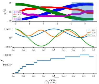
Figure 4: Performing a successful and low-cost bit swap: (Top) Ensemble averages, conditioned on initial memory state, of the fluxes and their conjugate momenta. Line width tracks the distribution’s variance. The shaded region indicates timescales that are potentially successful swap operations. These are probed more closely in the bottom two plots. (Middle) Ensemble averaged work, kinetic energy, and conjugate momentum in the $\varphi_{\text{dc}}$ coordinate. Note that work minima occur only at whole-integer oscillations of the momentum. Each dataset is scaled to its maximum value, so that it saturates at $1$. This emphasizes the qualitative relationships rather than the quantitative. (Bottom) Computational fidelity $f$ of the swap, approaching a perfect swap.

Figure 4 showcases this by displaying the behavior observed during simulations near the ideal timescale. The local work minima coincide with local minima in the average kinetic energy, but not every kinetic energy minimum coincides with a work minimum. While there are kinetic energy minima every half-integer oscillation in $\varphi_{\text{dc}}$, only integer multiples of $\varphi_{\text{dc}}$ oscillations yield minimum work.

The equations of motion governing the system are stochastic, dissipative, and nonlinear, so the frequencies of the different oscillations $\omega,\omega_{dc}$ are nontrivial nonlinear stochastic mappings of device parameters, initial positions, and protocol parameters. They are not easily determined analytically. However, they change smoothly with small changes in the parameters they depends on. Thus, we were able to use an algorithmic approach to find the timescales that yield local minima and explore the regions surrounding them.

III.3 Physically-Calibrated Bit Swap

We are most interested in the effect of parameters that are least constrained by fabrication. And so, all simulations assume constant fabrication parameters with $I_{+}$, $R$, and $C$ set to $2.0\text{\,}\mathrm{\SIUnitSymbolMicro A}$, $371\text{\,}\mathrm{\SIUnitSymbolOhm}$, and $4.0\text{\,}\mathrm{nF}$, respectively. To explore how the $I_{-}$ asymmetry affects work cost, we simulated protocols with both a nearly-symmetric device ($I_{-}=$7\text{\,}\mathrm{nA}$$) and a moderately-asymmetric device ($I_{-}=$35\text{\,}\mathrm{nA}$$). Given devices with the parameters above, what values of the other parameters yield protocols with minimum work cost? This involves a twofold procedure. First, create a circuit architecture by setting $L$ and $\gamma$, thus fully specifying the device; details in Appendix E. Second, determine the ideal protocols for that combination of device parameters.

III.4 Computational Fidelity

To determine the best successful protocol, we must define what a successful bit swap is. First, we set a lower bound for the fidelity $f$: $f\geq 0.99$. We define $f$ over an ensemble of $N$ independent trials as: $f=1-N_{e}/N$, with $N_{e}$ counting the number of failed trials, trials for which $\text{sign}[\varphi(t=0)]=\text{sign}[\varphi(t=\tau)]$. Second, the distribution over both $\varphi(t=\tau)$ and $\varphi(t=0)$ must be bimodal with clear and separate informational states. The criteria used for this second condition is:

$$\langle\varphi<0\rangle+3\sigma_{\varphi<0}<\langle\varphi>0\rangle-3\sigma_{\varphi>0}~{},$$ (3)

were $\sigma_{s}$ and $\langle s\rangle$ are standard deviations and means of $\varphi$ conditioned on statement $s$ being true.

The final choice concerns the initial distribution from which to sample trial runs. For this, we used the equilibrium distribution associated with $V^{\text{store}}$ with the environmental temperature set to satisfy $k_{\text{B}}T=0.05U_{0}$. Here, we ensure fair comparisons between different parameter settings by fixing a relationship between the potential’s energy scale and that of thermal fluctuations. This resulted in temperatures from $400-1400$ mK, though it is possible to create superconducting circuits at much higher temperatures [35, 36, 37, 38] using alternative materials.

Sampling initial conditions from a thermal state assumes no special intervention created the system’s initial distribution. We only need wait a suitably long time to reach it. Moreover, this choice is no more than an algorithmic way to select a starting distribution. It is not a limitation or restriction of the protocol. Indeed, if some intervention allowed sampling initial conditions from a lower-variance distribution, it could be leveraged into even higher performance.

IV Performance

Appendix E lays out the computational strategy used to find minimal $\langle W\rangle$ implementations among the protocols that satisfy the conditions above. Since the potential is held constant between $t=0$ and $t=\tau$, work is only done when turning $V^{\text{comp}}$ on at $t=0$ and turning it off at $t=\tau$. The ensemble average work done at $t=0$ is $W_{0}\equiv\langle V^{\text{comp}}(\varphi(0),\varphi_{\text{dc}}(0))-V^{\text{store}}(\varphi(0),\varphi_{\text{dc}}(0))\rangle$ and returning to $V^{\text{comp}}$ at time $\tau$ costs $W_{\tau}\equiv\big{\langle}V^{\text{store}}(\varphi(\tau),\varphi_{\text{dc}}(\tau))-V^{\text{comp}}(\varphi(\tau),\varphi_{\text{dc}}(\tau))\big{\rangle}$. Thus, the mean net work cost is the sum $\langle W\rangle=W_{0}+W_{\tau}$. As we detail shortly, this yielded large regions of parameter space that implement bit swaps at sub-Landauer work cost. This result and others demonstrate the notable and desirable aspects of momentum computing: accuracy, low thermodynamic cost, and high speed. Let’s recount these one by one.

IV.1 Accuracy

Tradeoffs between a computation’s fidelity and its thermodynamic cost are now familiar—an increase in accuracy comes at the cost of increased $W$ or computation time [39, 40, 41, 42, 43, 44]. These analyses conclude that accuracy generally raises computation costs.

Momentum computing does not work this way. In fact, it works in the opposite way. The low cost of a momentum computing protocol comes from controlling the distribution over the computing system’s final state. Due to this, fidelity and low operation cost are not in opposition, but go hand in hand, as Figs. 4 and 5 demonstrate.

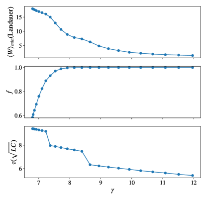
Figure 5: Performance of the minimum work protocol as $\gamma$, the ratio of device inductances, goes from a region where the computation fails ($f<0.99$) to a region of perfect fidelity ($f=1.0$). Note that in the parameter space region in which the computation becomes successful, the work costs decrease as the fidelity approaches unity. Finally, $\tau$ decreases as the work cost minimizes to $\approx 1$ Landauer—showing that the work cost does not display $1/\tau$ adiabatic compute-time scaling. The parameter $\gamma$ controls the starting parameters for the suite of simulations represented by each data point and should not be read as the primary independent variable responsible for the behavior. Rather, the plots show $\tau$, $f$, and $\langle W\rangle_{min}$ evolving jointly to more preferable values.

IV.2 Low Thermodynamic Cost

Conventional computing, based on transistor-network steady-state currents, operates nowhere near the theoretical limit of efficiency for logical gates. Even gates in Application Specific Integrated Circuits (ASICs) designed for maximal efficiency operate on the scale of $10^{4}-10^{6}$ Landauers [45, 46]. The physically-calibrated simulations described above achieved average costs well below a Landauer for a wide range of parameter values with an absolute minimum of $\langle W\rangle_{\text{min}}=0.43$ Landauers, as shown in Figure 6 (left). For the less-ideal asymmetric critical-current device (right panel), the cost increases to only $\langle W\rangle_{\text{min}}=0.60$ Landauers. And, the bulk of the protocols we explored operated at $<10$ Landauers. Altogether, the momentum computing devices operated many orders of magnitude lower than the status quo. Moreover, the wide basins reveal robustness in the device’s performance: an important feature for practical optimization and implementation.

IV.3 High Speed

Paralleling accuracy, the now-conventional belief is that computational work generally scales inversely with the computation time: $W\sim 1/\tau$ [39, 47, 48, 49]. Again, this is not the case for momentum computing, as Figs. 4 and 5 demonstrate. Instead, there are optimal times $\tau^{*}$ that give local work minima and around which the work cost increases.

Optimal $\tau^{*}$s are upper bounded: the devices must operate faster than particular timescales—timescales determined by the substrate physics. The bit swap’s low work cost requires operating on a timescale faster than the rates at which the system exchanges energy and information with the environment. Thus, momentum computing protocols have a speed floor rather than a speed limit.

However, even assuming perfect thermal isolation there is a second bound on $\tau^{*}$. The computation must terminate before the initially localized ensemble—storing the memory—decoheres in position space due to dispersion. For our JJ device this is the more restrictive timescale. Due to local curvature differences in the potential, the initially compact state-space regions corresponding to peaks of the storage potential’s equilibrium distribution begin to decohere after only one or two oscillations. Once they have spread to cover both memory states, the stored information is lost. This means it is most effective to limit the duration of the swap to just a half-oscillation of the $\varphi$ coordinate. For our devices, this typically corresponds to operating on timescales $<15$ ns.

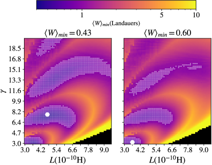
Figure 6: Thermodynamic energy cost $\langle W\rangle_{\text{min}}$ for momentum-computing bit-swap over $5,120$ parameter combinations of $L$ and $\gamma$. (Left) Slightly asymmetric device with $I_{-}=$7\text{\,}\mathrm{nA}$$ gives the overall minimum $\langle W\rangle_{\text{min}}=0.43$ Landauers (large solid white circle). (Right) Substantially asymmetric device with $I_{-}=$35\text{\,}\mathrm{nA}$$ gives the overall minimum $\langle W\rangle_{\text{min}}=0.60$ Landauers (large solid white circle). (Both) Small white circles indicate parameter values with protocols yielding $\langle W\rangle_{\text{min}}<1$ Landauer. Black squares (lower right in each) represent parameter values where no successful swap was accomplished. Note that when the asymmetry is low, it can effectively be offset by the parameter $\varphi_{x}$, but for higher asymmetry, protocols that cost less than $1$ Landauer are less common.

V Related Work

Reversible computing implementations of various operations have been proposed many times over many decades. Perhaps the most famous is the Fredkin billiards implementation [18]. While ingenious, it suffers from inherent dynamical instability (deterministic chaos) and cannot abide any interactions with the environment. At the other end of the spectrum is a family of superconducting adiabatic implementations [50, 51, 52, 53, 54, 55, 56, 57]. These are low cost in terms of dissipation and are stable, but they suffer from fundamental speed limits due to the adiabaticity requirement: $\langle W\rangle\propto 1/\tau$.

Other recent implementations [58, 59, 60] of reversible logic using JJs are more akin to the proposal at hand, in that they require nearly-ballistic dynamics and attempt to recapture the energy used in a swap at the final step. While these implementations are markedly different, their motivation follows similar principles. Particularly, the framework for asynchronous reversible computing proposed in [59, 60] might serve as a testbed for momentum computing elements.

Another distinguishing feature of the present design is that the phenomenon supporting the computing is inherently linked to microscopic degrees of freedom evolving in the device’s phase space. This moves one closer to the ultimate goal of using reversible nanoscale phenomena as the primitives for reversible computing—a goal whose importance and difficulty were recognized by Ref. [61]. Working directly with the underlying phase space also allows incorporating the thermal environment. And, this facilitates characterizing the effect of (inevitable) imperfect isolation from the environment.

It is worth noting the similarity between the optimal timescales $\tau^{*}$ and the principal result in Ref. [62] in which a similar local minima emerges when comparing thermodynamic dissipation to computation time. These minima also come from certain matching conditions between the rate of thermalization and the system’s response time to its control device. Another qualitatively similar result [63] found faster operation could lead to reduced errors in overdamped JJs under periodic driving. These similarities could point to a more general principle at play.

VI Conclusion

Our detailed, thermodynamically-calibrated simulation of microscopic trajectories demonstrated that momentum computing can reliably (i) implement a bit swap at sub-Landauer work costs at (ii) nanosecond timescales in (iii) a well-characterized superconducting circuit.

These simulations served two main purposes. The first highlights momentum computing’s advantages. The proposed framework uses the continuum of momentum states to serve as the auxiliary system that allows a swap. In doing so, it eliminates the associated tradeoffs between energetic, temporal, or accuracy costs that are commonly emphasized in thermodynamic control analyses [42, 39, 40, 41]. Momentum computing protocols are holistic in that low energy cost, high fidelity, and fast operation times all come from matching parallel constraints rather than competing ones.

The second purpose points out key aspects of the proposed JJ circuit’s physics. The simulations reveal several guiding principles—those that contribute most to decreasing work costs for the proposed protocols. The system is so underdamped that thermal agitation is not the primary cause of inefficiency. The two main contributors are (i) the appearance of dispersive behavior in the dynamics of an initially-coherent region of state space and (ii) asymmetries inherent to the device that arise from differing critical currents in the component superconducting JJ elements. Notably, if the elements are very close to each other in $I_{c}$, then symmetry can be effectively restored by setting the control parameter $\varphi_{x}$ to counteract the difference. However, the more asymmetry, the harder it is to find ultra low-cost protocols; cf. Fig. 6 left and right panels. Note, too, that initial-state dispersion can be ameliorated by using a $V^{\text{comp}}$ that is as harmonic (quadratic) as possible. However, this typically requires lower inductance $L$, possibly complicating circuit fabrication. Additionally, the potential-well separation parameter $\beta$’s linear dependence on $L$ hinders the system’s ability to create two distinct states during information storage. Though these tradeoffs are complicated, our simulations suggest that dispersion can be controlled, yielding swap protocols with even lower work costs.

Since the protocol search space is quite high-dimensional and contains many local-minima, we offer no proof that the protocols found give the global work minimum. Very likely, the thermodynamic costs and operation speed of our proposed JJ momentum computing device can be substantially improved using more sophisticated parameter optimization and alternative materials. Even with the work cost as it stands, though, sub-Landauer operation represents a radical change from transistor-based architectures. One calibration for this is given in the recent stochastic thermodynamic analysis of a NOT gate composed of single-electron-state transistors [24] that found work costs $10^{4}$ times larger.

Note, too, that running at low temperatures requires significant off-board cooling costs, as required in superconducting quantum computing. Our current flux qubit implementation requires operating at liquid He temperatures [19, 20]. However, there are also JJs that operate at $N_{2}$ temperatures, promising system cooling costs that would be $2$ to $3$ orders of magnitude lower [35, 36, 37, 38].

Additionally, the physics necessary to build a momentum computing swap—underdamped behavior and controllable multiwell dynamics—is far from unique to superconducting circuits. As an example, nanoelectromechanical systems (NEMS) are another well-known technology that is scalable with modern microfabrication techniques. NEMS provide the needed nonlinearity for multiple-well potentials, are extremely energy efficient, and have high Q factors even while operating at room temperature [64, 65, 66]. Momentum computing implemented with NEMS rather than superconductors completely obviates the cooling infrastructure and so may be better suited for large-scale implementations.

That said, the JJ implementation at low temperatures augmented with appropriate calorimetry will provide a key experimental platform for careful, controlled, and detailed study of the physical limits of the thermodynamic costs of information processing. Thus, these devices are necessary to fully understand the physics of thermodynamic efficiency. And so, beyond technology impacts, the proposed device and protocols provide a fascinating experimental opportunity to measure energy flows that fluctuate at GHz timescales and at energy scales below thermal fluctuations. Success in these will open the way to theoretical investigations of the fundamental physics of information storage and manipulation, time symmetries, and fluctuation theorems [43, 67].

Appendix A The Landauer: A Standard Candle for Thermodynamic Computation

A long and checkered history underlies the physics of information and energy, arguably originating in the paradox of Maxwell’s Demon [68]. Most recently, though, the paradigm of thermodynamic computing emerged to frame probing their limits [69]. In this setting, Landauer’s Principle says that $k_{\text{B}}T\ln 2$ energy units must be expended to erase a single bit of information. Beyond erasure, though, his Principle also stands as a challenge—Can conventional computing paradigms operate at sub-Landauer scales? It seems not. Landauer’s theory and follow-on results [70, 71, 72] and recent experiments [42, 73] verified the lower bound.

To apply more broadly, Landauer’s Principle generalizes to $W\geq k_{\text{B}}T\Delta H$, where $\Delta H$ is the change in Shannon entropy between a computational system’s initial and final information-bearing states [74, 71, 75]. Despite the Principle’s generalization beyond bit erasure, the Landauer scale remains a familiar reference point for the energy costs of binary operations; its familiar use coming at the expense of ignoring specifics of any given logical operation [44].

An efficient bit-swap operation, for example, has zero generalized Landauer cost, as it is logically reversible. However, since many thermodynamic computing architectures do not have access to dynamics that can accomplish reversible computing efficiently, the Landauer scale provides a common reference to compare gate performance across physical substrates and design paradigms. It also facilitates comparing across substrates that operate at different temperatures. Table 1 lists thermodynamic energies for a range of physical environments. Table 2 gives Landauer work energies for various information processing operations in environments and at temperatures where thermodynamic computers operate.

Appendix B Limits of Stochastic Thermodynamics for Information Processing

Stochastic thermodynamics [26, 27] has been the predominant framework for analyzing the thermodynamic costs of stochastic mappings. It assumes the memory state $m$ obeys stochastic Markovian dynamics: continuous-time Markov chains (CTMCs), where the state distribution $\vec{p}(t)$ changes continuously as a function of itself: $\dot{\vec{p}}(t)=f(\vec{p},t)$. The resulting dynamics are necessarily represented by a master equation over the memory-state distribution $\dot{\vec{p}}(t)=\mathbf{A}(t)\vec{p}(t)$ [76]. This framework is powerful, yielding great insight into physical processes when its assumptions are met.

The framework, however, does not apply to momentum computing. To appreciate why, consider justifying Markovian dynamics over memory states. Assume a microscopic physical system $\mathcal{S}$ that serves as a computational substrate. While allowing the universe to be deterministic, $\mathcal{S}$ can exhibit stochastic dynamics since it represents only a portion of the partially-observed universe. The very typical assumption that $\mathcal{S}$’s local environment acts as a large weakly-coupled heat bath with quickly relaxing degrees of freedom yields dynamics on $\mathcal{S}$ that are also Markovian and, therefore, can be represented by CTMCs.

However, computationally-useful memory states are not the CTMC-obeying microstates of $\mathcal{S}$, but a set $\mathcal{M}$ of mesostates that represent coarse-graining over $\mathcal{S}$. It is possible, depending on the variables or timescales of interest, that this coarse-graining ignores only rapidly-relaxing subsystems of $\mathcal{S}$. Then $\mathcal{M}$ inherits the Markov property that governs the microstates [26]. This strategy—coarse graining over physical degrees of freedom irrelevant to the dynamics—is analogous to establishing $\mathcal{S}$ as a stochastic, Markovian subsystem of the universe. A straightforward example of this case is when $\mathcal{M}$ consists of positional degrees of freedom and $\mathcal{S}$ evolves by overdamped Langevin dynamics.

When implementing momentum computing, however, the coarse-graining yielding $\mathcal{M}$ is applied over hidden microstates that contain dynamically relevant information not determined from $\mathcal{M}$’s instantaneous realizations. As a consequence, the dynamic over the coarse-grained states is not Markovian. CTMCs cannot be used. A straightforward example of this arises when $\mathcal{M}$ consists of positional degrees of freedom and $\mathcal{S}$ evolves by underdamped Langevin dynamics. On the downside, a general analytical treatment of such partially-observed systems (continuous-time hidden Markov chains) is highly nontrivial [77, 27, 78, 79]. On the upside, the possibility of hidden states allows for substantially more general forms of computation. As the results here showed, the benefits of this expanded space are quite substantial.

Note that the bit swap computation is, in general, problematic to implement using CTMCs since input-output mappings whose determinants are negative are disallowed when memory-state dynamics are restricted to obey CTMCs. Formally, auxiliary systems can be added to the set of memory states. Done correctly this again permits using CTMCs in the augmented state space to accomplish the computation [76].

However, physically-embedded computations do not generally allow the required perfect control over the system Hamiltonian. Indeed, one need look no further than the present work to see how nontrivial it is to implement an operation as simple as a harmonic oscillation in a physically-realistic device.

Moreover, adding auxiliary subsystems increases state-space dimension and complicates control apparatus and control protocols. Due to the increased complication, in many settings, adding auxiliary dimensions is simply not physically possible. On top of this, the timescale of these augmented computations must be longer than the equilibration time of the auxiliary systems and thermal environment. In this way, adding auxiliary systems imposes additional speed limits to computations. In short, adding auxiliary subsystems addresses the shortfalls of CTMCs, but does not sidestep their fundamental limitations.

We illustrate this by considering an efficient bit swap implemented via a Markovian embedding. First, it augments the system with an unoccupied auxiliary state $A$ to serve as a transient memory. It then quasistatically translates memory state $0$ to $A$, while memory state $1$ is translated to $0$. Finally, it quasistatically translates $A$ to $1$.

Quasistatic processes cost arbitrarily little work, but they take arbitrarily-long times. To compute faster ($\tau\to 0$), the work cost will diverge as $1/\tau$ [39, 47, 48, 49]. Increasing fidelity requires raising the scale of the barrier separating the states. Doing so, though, increases the energetic cost at a given computational speed; maintaining the same work cost, then, requires slowing the operation. In short, the trade-offs in Markovian embedding complicate design and, more to the point, reduce performance.

Appendix C Flux Qubit Dimensionless Equations of Motion

In terms of the dimensional degrees of freedom, the flux qubit equations of motion are:

$$\ddot{\widehat{\varphi}} =-\frac{2}{RC}\dot{\widehat{\varphi}}-\frac{1}{C}\partial_{\widehat{\varphi}}U(\widehat{\varphi},\widehat{\varphi}_{dc})$$ (4)

$$\ddot{\widehat{\varphi}}_{dc} =-\frac{2}{RC}\dot{\widehat{\varphi}}_{dc}-\frac{4}{C}\partial_{\widehat{\varphi}_{dc}}U(\widehat{\varphi},\widehat{\varphi}_{dc})~{},$$ (5)

where the dimensional $\widehat{\varphi}$s are related to the main text’s dimensionless fluxes and phases by the magnetic flux quantum $2\pi/\Phi_{0}$. With the addition of thermal noise, the Langevin equation is:

$$dv_{i}=-\frac{\nu_{i}}{m_{i}}v_{i}dt-\frac{1}{m_{i}}\partial_{x_{i}}U(x)dt+\frac{1}{m_{i}}r(t)\sqrt{2\nu_{i}\kappa dt}~{},$$ (6)

where $\kappa\equiv k_{B}T$. Matching these variables to the equations of motion yields:

$$x =\left(\widehat{\varphi},\widehat{\varphi}_{dc}\right)$$ (7)

$$v =\left(\dot{\widehat{\varphi}},\dot{\widehat{\varphi}}_{dc}\right)$$ (8)

$$m =\left(C,\frac{C}{4}\right),~{}\text{and}$$ (9)

$$\nu =\left(\frac{2}{R},\frac{1}{2R}\right)~{},$$ (10)

where subscript $i$ has been dropped in favor of a vector representation.

The task is to write each physical quantity $z$ in terms of a dimensional constant and dimensionless variable by defining scaling factors according to the following prescription: $z\equiv z^{\prime}z_{c}$, where $z_{c}$ is a dimensionful constant.

Setting $m_{c}=C$ and $\nu_{c}=1/R$ are obvious choices. Additionally, since the potential factors into $U=U_{0}\times U^{\prime}(\frac{2\pi}{\Phi_{0}}\cdot x)$, a good choice for positional scaling is $x_{c}=\Phi_{0}/2\pi$.

It is advantageous to write nondimensional kinetic energies as $\frac{1}{2}m^{\prime}v^{\prime 2}$ without additional scaling factors. This means setting the energy scaling as:

$$E_{c}=m_{c}\frac{x^{2}_{c}}{t^{2}_{c}}~{}.$$ (11)

This does not uniquely determine the energetic scale, since $t_{c}$ is still free. The two obvious choices are to scale to the temperature—$KE^{\prime}=1$ corresponds to $k_{B}T$ units of dimensional energy—or to the potential energy scale—$KE^{\prime}=1$ corresponds to $U_{0}$ units of dimensional energy. Choosing the latter yields:

$$E_{c} =U_{0}=m_{c}\frac{x^{2}_{c}}{t^{2}_{c}}\text{~{}and}$$ (12)

$$\frac{x_{c}^{2}}{L} =m_{c}\frac{x^{2}_{c}}{t^{2}_{c}}~{}.$$ (13)

Evidently, the timescale is $t_{c}=\sqrt{LC}$, which is a workable timescale for our purposes given that the dynamics of interest happen on the scale of $\tau\approx\omega_{LC}$. Setting the timescale to the potential energy rather than the thermal energy may well become common practice in simulating momentum computation, since protocols must be timed precisely with respect to the dynamics of the potential energy surface.

The Langevin equation, in terms of the nondimensional quantities defined above, becomes:

$$dv^{\prime}\frac{x_{c}}{t_{c}} =-\frac{\nu^{\prime}\nu_{c}}{m^{\prime}m_{c}}v^{\prime}x_{c}dt^{\prime}-\frac{1}{m^{\prime}m_{c}}\left(\frac{U_{0}}{x_{c}}\partial_{x^{\prime}}U^{\prime}(x^{\prime})\right)t_{c}dt^{\prime}$$ (14)

$$\quad+\frac{1}{m^{\prime}m_{c}}r(t)\sqrt{2\nu^{\prime}\nu_{c}E_{c}\kappa^{\prime}t_{c}dt^{\prime}}~{}.$$

Simplifying algebra then yields:

$$dv^{\prime} =-\frac{\sqrt{LC}}{RC}\frac{\nu^{\prime}}{m^{\prime}}v^{\prime}dt^{\prime}-\frac{1}{m^{\prime}}\partial_{x^{\prime}}U^{\prime}(x^{\prime})dt^{\prime}$$ (15)

$$\quad+\left(\frac{L}{R^{2}C}\right)^{1/4}\frac{\sqrt{\nu^{\prime}\kappa^{\prime}}}{m^{\prime}}r(t)\sqrt{2dt^{\prime}}~{}.$$

Finally, we define $\lambda$, $\theta$, and $\eta$ as nondimensional parameters that serve as our dimensionless Langevin coefficients. This yields the Langevin equation for the simulations detailed in Appendix E:

$$dv^{\prime}=-\lambda v^{\prime}dt^{\prime}-\theta\partial_{x^{\prime}}U^{\prime}+\eta r(t)\sqrt{2dt^{\prime}}~{},$$ (16)

with:

$$\lambda =\frac{\sqrt{LC}}{RC}\frac{\nu^{\prime}}{m^{\prime}},$$ (17)

$$\theta =\frac{1}{m^{\prime}},~{}\text{and}$$ (18)

$$\eta =\sqrt{\frac{\lambda\kappa^{\prime}}{m^{\prime}}}~{},$$ (19)

where:

$$x^{\prime} =(\varphi,\varphi_{dc}),$$ (20)

$$v^{\prime} =\frac{d}{dt^{\prime}}x^{\prime},$$ (21)

$$\nu^{\prime} =(2,1/2),$$ (22)

$$m^{\prime} =(1,1/4),~{}\text{and}$$ (23)

$$\kappa^{\prime} =\frac{k_{B}T}{U_{0}}~{}.$$ (24)

Appendix D Effective Potential and Simulation Details

We consider two cases: critical-current symmetric and asymmetric JJ pairs.

D.1 Symmetric Approximation

We can obtain reasonable estimates for good $\varphi_{\text{xdc}}$ values by assuming a perfectly symmetric device $\delta\beta=0$. Furthermore, we also set $\varphi_{x}=0$ for all cases. This allows two symmetric wells on either side of $\varphi=0$. In practice, since $\delta\beta\neq 0$ in a real device, $\varphi_{x}$ would be calibrated to compensate for the asymmetry; see Sec. D.2.

In the symmetric case, the potential splits into two components—periodic and quadratic:

$$\beta\cos\varphi\cos\frac{\varphi_{\text{dc}}}{2}+\frac{1}{2}\varphi^{2}+\frac{\gamma}{2}(\varphi_{\text{dc}}-\varphi_{\text{xdc}})^{2}~{}.$$ (25)

The periodic term allows for multiple minima, while the quadratic terms force the dynamical variables to stay close to their respective parameters. This localization means we focus only on the the area near $\varphi=\varphi_{x}$ and $\varphi_{\text{dc}}=\varphi_{\text{xdc}}$.

To employ the potential most flexibly, we must characterize the relevant fixed points that occur in this region. Following Refs. [19, 33], we choose to search in the domain $-\pi<\varphi<\pi$ and $-2\pi<\varphi_{\text{dc}}<0$. Fixed points occur when all components of the gradient vanish:

$$\partial_{\varphi}U^{\prime} =-\beta\sin\varphi\cos\frac{\varphi_{\text{dc}}}{2}+\varphi=0$$ (26)

$$\partial_{{\varphi_{\text{dc}}}}U^{\prime} =-\frac{\beta}{2}\sin\frac{\varphi_{\text{dc}}}{2}\cos\varphi+\gamma(\varphi_{\text{dc}}-\varphi_{\text{xdc}})=0$$ (27)

The first condition is met whenever $\varphi=0$ and, also, when $\frac{\varphi}{\beta\sin\varphi}=\cos\frac{1}{2}\varphi_{\text{dc}}$. Consider the case where $\varphi=0$—the “central” fixed point. To find the $\varphi_{\text{dc}}$ location of the fixed point $\varphi^{0}_{dc}$, we look to the gradient’s second term. This yields the condition:

$$\varphi_{\text{dc}}^{0}-\frac{\beta}{2\gamma}\sin\frac{\varphi_{\text{dc}}^{0}}{2} =\varphi_{\text{xdc}}$$ (28)

$$F^{0}(\varphi_{\text{dc}}=\varphi_{\text{dc}}^{0},\beta,\gamma) =\varphi_{\text{xdc}}~{}.$$

The central fixed point occurs close to the parameter $\varphi_{\text{xdc}}$, but is offset by a value $\leq\beta/2\gamma$.

The equation above can be solved numerically with ease to find the location of the central fixed point. To classify the fixed point, we look at the Hessian. While the general expression for the eigenvalues is rather verbose, the case where $\varphi=0$ simplifies to:

$$\lambda_{1} =-\beta\cos\frac{\varphi_{\text{dc}}^{0}}{2}+1$$ (29)

$$\lambda_{2} =\gamma-\frac{\beta}{4}\cos\frac{\varphi_{\text{dc}}^{0}}{2}~{}.$$ (30)

$\lambda_{2}>0$ as long as $\gamma>\beta/4$. And, since we assume $\gamma>\beta$, this condition is always met. Thus, this fixed point is either a saddle point or a minimum based on whether $\varphi_{\text{dc}}^{0}$ is greater or less than $\varphi_{\text{dc}}^{c}\equiv-2\cos^{-1}\frac{1}{\beta}$, respectively. (We only use the negative branch of $\cos^{-1}$ due to the domain of $\varphi_{\text{dc}}$.) See Fig. 7 for an example of the behavior of the central fixed point for typical parameters.

We can also find an expression for $\varphi_{\text{xdc}}^{c}(\beta,\gamma)\equiv F^{0}(\varphi_{\text{dc}}=\varphi_{\text{dc}}^{c})$, the critical value of the control parameter at which the central fixed point transitions between a saddle point and a minimum:

$$\varphi_{\text{xdc}}^{c}(\beta,\gamma) =\varphi_{\text{dc}}^{c}-\frac{\beta}{2\gamma}\sin\frac{\varphi_{\text{dc}}^{c}}{2}$$

$$=-2\cos^{-1}\frac{1}{\beta}+\frac{\beta}{2\gamma}\sqrt{1-\frac{1}{\beta^{2}}}~{}.$$ (31)

Naively, the best strategy to form a low cost protocol is to take values of $\varphi_{\text{xdc}}$ just above and below $\varphi_{\text{xdc}}^{c}$. However, there are several factors that introduce complications. For one, the energy scale separating the two wells when $\varphi_{\text{xdc}}\approx\varphi_{\text{xdc}}^{c}$ is very small and it will typically be overwhelmed by thermal energy at the temperatures of interest ($400-1400$ mK). A second is that the approximation of $\delta\beta=0$ actually has a most pernicious effect near $\varphi_{\text{xdc}}^{x}$. (This is discussed in Sec. D.2.)

Finally, we have yet to consider the other fixed points at $\varphi\neq 0$. Doing so reveals that sometimes $\varphi_{\text{xdc}}^{c}$ corresponds to a subcritical pitchfork bifurcation—yielding a potential with a third (undesirable) minimum rather than a single one.

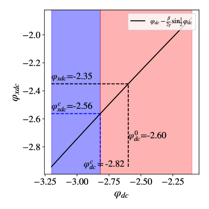
Figure 7: Fixed point at $\varphi=0$ in an ideal device with $\beta=6.2$ and $\gamma=12.0$: Red (Blue) background indicates regions where the fixed point is a saddle point (local minimum). For example, if $\varphi_{\text{xdc}}=-2.35$, the central fixed point is a saddle point at $\varphi_{\text{dc}}=-2.6$. To find a stable fixed point at $\varphi=0$, a control parameter less than $\varphi_{\text{xdc}}^{c}$ is necessary, which falls at $-2.56$ in the example above.

When $\varphi\neq 0$ we can rewrite Eqs. (26) and (27):

$$\frac{\varphi}{\beta\sin\varphi} =\cos\frac{1}{2}\varphi_{\text{dc}}$$ (32)

$$\frac{\beta}{4\gamma}\sin\frac{\varphi_{\text{dc}}}{2}\cos\varphi-\frac{1}{2}\varphi_{\text{xdc}} =\frac{1}{2}\varphi_{\text{dc}}~{}.$$ (33)

The potential is symmetric, so these fixed points come in pairs $\varphi^{\pm}$. Substituting $\varphi_{\text{dc}}/2=-\cos^{-1}(\varphi^{\pm}/\beta\sin\varphi^{\pm})$ into the second equation yields the following for $\varphi^{\pm}$:

$$\varphi_{\text{xdc}} =\frac{\beta}{2\gamma}\sqrt{1-\left(\frac{\varphi^{\pm}}{\beta\sin\varphi^{\pm}}\right)^{2}}\cos\varphi^{\pm}-2\cos^{-1}\frac{\varphi^{\pm}}{\beta\sin\varphi^{\pm}}$$ (34)

$$\varphi_{\text{xdc}} =F^{\pm}(\varphi=\varphi^{\pm},\beta,\gamma)~{}.$$ (35)

Note that the sign changes due to the domain restriction of $\varphi_{\text{dc}}$. Figure 8 shows how these fixed points behave as $\beta$, $\gamma$, and $\varphi_{\text{xdc}}$ change. The value of $\varphi_{\text{xdc}}$ tangent to the curve when $\varphi=0$ corresponds to the critical control parameter value $\varphi_{\text{xdc}}^{c}$, which can be seen by verifying $\lim_{\varphi\to 0}F^{\pm}(\varphi)=\varphi_{\text{xdc}}^{c}$.

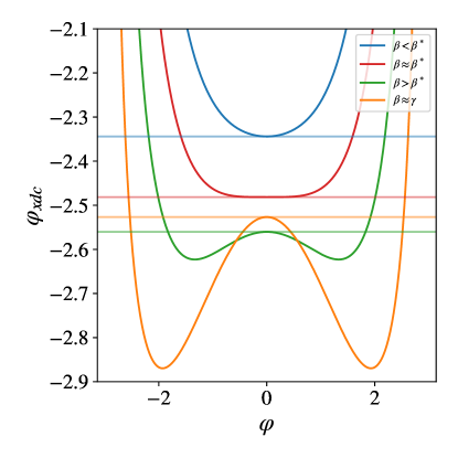
Figure 8: $\varphi\neq 0$ fixed points appear when the value of the function plotted equals the external $\varphi_{\text{xdc}}$ parameter. Note that for some $\beta$ and $\gamma$ combinations, there is a qualitatively different behavior. Especially for larger $\beta$, there is a coexistence region of three potential minima. For the $\beta\approx\gamma$ example, one would want to set $\Delta C>0.5$ to make sure $V^{\text{comp}}$ falls well outside of the three minima range. Horizontal lines show the values of $\varphi^{c}_{xdc}$. (See Appendix E.)

As a last note, different values of $\beta$ and $\gamma$ have qualitatively different fixed point profiles depending on whether the central fixed point undergoes a supercritical or subcritical pitchfork bifurcation when $\varphi_{\text{xdc}}=\varphi_{\text{xdc}}^{c}$. The critical value $\beta^{*}$ where the bifurcation of the central fixed point transitions between being supercritical and subcritical is given by:

$$\lim_{\varphi\to 0}\partial^{2}_{\varphi}F^{\pm}(\varphi,\beta^{*},\gamma)=0~{}.$$ (36)

Once again, the full derivative is quite verbose. However, taking the limit $\varphi\to 0$ gives:

$$\frac{\sqrt{\beta^{*^{2}}-1}}{6\beta^{*^{2}}}\left(-3\beta^{*^{2}}+4\gamma+2\right) =0$$ (37)

$$\beta^{*} =\sqrt{\frac{4\gamma+2}{3}}~{}.$$ (38)

Interestingly, when $\beta>\beta^{*}$, there is always a parameter space region with three distinct minima. This might be useful, in fact, for single-bit computations that require more states. For bit swap, though, the goal is for the system to jump between a $V^{\text{store}}$ with $2$ minima and a $V^{\text{comp}}$ with a single minimum (see Figure 10). And so, care must be taken to avoid the three-minima regions when $\beta>\beta^{*}$.

D.2 $\delta\beta\neq 0$

The device just considered is ideal. In reality $\delta\beta\neq 0$, and exact analytic work is much less fruitful. Introducing the asymmetric terms augments the potential:

$$U_{\text{asym}}(\varphi,\varphi_{x},\delta\beta,\varphi_{\text{dc}})=\frac{1}{2}\varphi_{x}^{2}-\varphi\varphi_{x}-\delta\beta\sin\varphi\cos\frac{\varphi_{\text{dc}}}{2}~{}.$$ (39)

In short, one must vary $\varphi_{x}$ to offset the effect of $\delta\beta$, provided a symmetric potential is preferred.

There are two obvious strategies to minimize the effects of asymmetry. Either a strategy that minimizes the effect of $U_{asym}$ at the central fixed point—the “min of mid” strategy—or at the fixed points at $\varphi^{\pm}$—the “min of max” strategy. It stands to reason that one uses the former to set $\varphi_{x}$ for $V^{\text{comp}}$ and the latter for $V^{\text{store}}$.

The “min of mid” strategy is easy to implement. Simply set the derivative of $\partial_{\varphi}U_{asym}|_{\varphi=0}=0$, with the intent of having the asymmetrical part of the potential be as flat as possible near $\varphi=0$. Simple algebra yields: $\varphi_{x}=-\delta\beta\sin\varphi_{\text{dc}}/2$.

The “min of max” strategy requires numerical solution. First, note that the maximum value of $U_{asym}$ occurs when $\varphi=\varphi_{max}=\arccos(\frac{\varphi_{x}}{\delta\beta\sin.5\varphi_{\text{dc}}})$. Then, use a symbolic solver (e.g., SymPy’s nsolve function) to find the value of $\varphi_{x}$ that minimizes $U_{asym}(\varphi_{max},\varphi_{x},\delta\beta,\varphi_{\text{dc}})$.

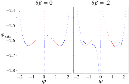
Figure 9: Fixed point bifurcation diagram for the (left) idealized $\delta\beta=0$ device and (right) a device with $\delta\beta=0.2$. Blue indicates stable minima and red saddle points. On the right plot, the $\delta\beta=0$ fixed points are plotted as well, with low opacity to help see the difference. The naive “minimum of maximum” strategy has been used to minimize the effect of $U_{asym}$. And, we can see that the symmetric approximation works fairly well as long as $|\varphi_{\text{xdc}}-\varphi_{\text{xdc}}^{c}|>.2$. It is likely that more evolved solution strategies will improve results.

Figure 9 shows that the effect of $\delta\beta\neq 0$ is, unsurprisingly, the most noticeable near the bifurcation of the central fixed point. For the bit swap, as described in Sec. II.2, we need only two different profiles for the potential: one in which we have two symmetric wells and one in which we have a single well placed midway between them. Thus, we must keep the $\varphi_{\text{xdc}}$ parameter sufficiently far away from $\varphi_{\text{xdc}}^{c}$. The strategy employed in the simulations described below always involves setting a minimum distance that $\varphi_{\text{xdc}}$ must be from $\varphi_{\text{xdc}}^{c}$, in order to avoid falling into the pitfalls described here.

Figure 10: (Left) $V^{\text{store}}$, the bistable storage potential. (Right) $V^{\text{comp}}$, the “banana-harmonic” potential. These potential energy profiles serve as qualitative pictures to represent prototypical computational and storage potentials, and do not represent any particularly favorable parameter set.

Appendix E Searching for Minimal-Work Bit Swaps

The following lays out the computational strategy to find low work-cost implementations.

We are most interested in the effect of parameters that are the most removed from fabrication, so all simulations assume JJ elements with $I_{+}$, $R$, and $C$ set to $2.0\text{\,}\mathrm{\SIUnitSymbolMicro A}$, $371\text{\,}\mathrm{\SIUnitSymbolOhm}$, and $4.0\text{\,}\mathrm{nF}$, respectively. To explore how asymmetry affects work cost, we simulated protocols with a nearly-symmetric device with $I_{-}=$7\text{\,}\mathrm{nA}$$, a moderately-symmetric device with $I_{-}=$35\text{\,}\mathrm{nA}$$, and an asymmetric device with $I_{-}=$60\text{\,}\mathrm{nA}$$. Additionally, $k_{\text{B}}T$ is always scaled to $U_{0}$, so that $\kappa^{\prime}\equiv k_{\text{B}}T/U_{0}=0.05$.

Given devices with the parameters above, what values of the remaining parameters yield protocols with minimum work cost? This involves a twofold procedure. First, create the circuit architecture by setting $L$ and $\gamma$ by hand; thus, fully specifying the device. Second, determine the ideal protocols for that combination of device parameters through simulation.

$L$’s order of magnitude was chosen from previous results [31, 32, 33, 34, 19, 20] to be $10^{-9}H$. Noting that a lower $L$ results in a more harmonic potential during computation, we set a minimum $L$ to be $0.3nH$. This is in order to stay within the parameter range for which $\beta>1$ and we can still use the analytic expressions derived above. To assure $\gamma>\beta$, $\gamma$ values were tested in the range $[3.0,20.0]$.

After choosing a pair of circuit parameters $L$ and $\gamma$, we turn to simulation. First, $V^{\text{store}}$ must be chosen by setting $\varphi_{x}^{\text{store}}$ and $\varphi_{\text{xdc}}^{\text{store}}$. This is done by calculating $\varphi_{\text{xdc}}^{\text{store}}\equiv\varphi_{\text{xdc}}^{c}+\Delta S$, where $\varphi_{\text{xdc}}^{c}(\gamma,\beta)$ is from Eq. (31). The parameter $\Delta S$ is initialized manually to a value $\Delta S^{*}$ when starting a new round of simulations. ($\Delta S^{*}=0.16$ was used in the heatmaps shown in Fig. 6.) Then, using the “min of max” method (Sec. D.2), we set $\varphi_{x}^{\text{store}}$.

Finally, $V^{\text{store}}$ is tested by sampling 50,000 states from $V^{\text{store}}$’s equilibrium distribution using a Monte Carlo algorithm. The resulting ensemble is verified by determining that it contains two well-separated informational states by asserting that:

$$\langle\varphi<0\rangle+3\sigma_{\varphi<0}<\langle\varphi>0\rangle-3\sigma_{\varphi>0}~{},$$ (40)

where $\langle s\rangle$ and $\sigma_{s}$ are means and standard deviations of $\varphi$ conditioned on $s$ being true. If the ensemble fails the test, $\Delta S$ is incremented and the process is repeated. If the ensemble succeeds, we have found a viable $V^{\text{store}}$.

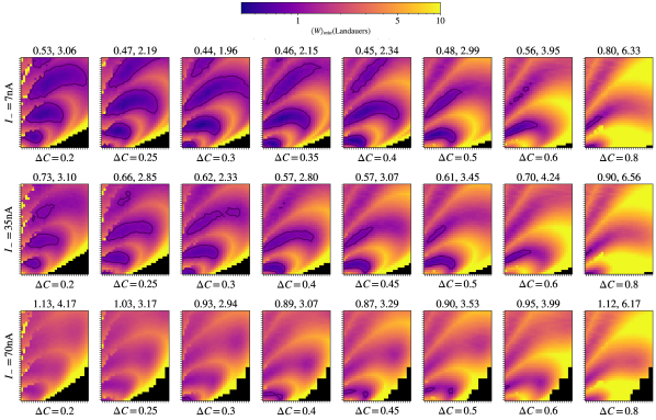
Figure 11: Thermodynamic performance under changing $\Delta C$ for devices with three different symmetry parameters: In each case, the $x$ axis variable is $L\in(0.3,1)$nH and the $y$ axis $\gamma\in(3,20)$. The numerical figures at the top of each panel are the minimum and average values of $\langle W\rangle_{\text{min}}$. The outlined (black line) regions represent pieces of parameter space where the minimal work protocols cost less than one Landauer. The simulations represented by each point in the heatmaps used $10,000$ samples from the equilibrium distribution. And, $1,200$ parameter sets were tested in each map.

Then, we move on to establish $V^{\text{comp}}$ by choosing $\varphi_{x}^{\text{comp}}$ and $\varphi_{\text{xdc}}^{\text{comp}}$. Similar to $\varphi_{\text{xdc}}^{\text{store}}$, $\varphi_{\text{xdc}}^{\text{comp}}\equiv\varphi_{\text{xdc}}^{c}-\Delta C$ with $\Delta C$ manually set. The value of $\Delta C$ does effect the eventual work cost, but the work costs vary smoothly, and a single value of $\Delta C$ tends to work well over a large parameter range. Manually setting a single value for $\Delta C$, rather than allowing it to adjust itself to fall into a local minimum, substantially reduces simulation run time. However, we expect that given more compute resources a wider range of sub-Landauer protocols will be discovered. Figure 11 shows the effect of changing $\Delta C$ for three different devices. Once $\Delta C$ is chosen, we use the “min of mid” (Sec. D.2) method to set $\varphi_{x}^{\text{comp}}$ and fully determine $V^{\text{comp}}$.

Next, a preliminary simulation is run to identify an approximate value of the computation time $\tau$. To make the simulation run quickly, the ensemble above is coarse-grained into two partitions based on whether $\varphi>0$ or $\varphi<0$. Then, each partition is coarse-grained again into $\approx 250$ representative points through histogramming. A Langevin simulation is run over the histogram data, exposing it to $V^{\text{comp}}$ for a time $\mathcal{O}(10)\sqrt{LC}$. This ensures capturing the time with the best bit swap. Next, weighting the simulation results by histogram counts within each partition, we obtain conditional averages for an approximation of the behavior over the entire ensemble. These averages are parsed for a set of times at which there are indications of a successful and low-cost bit swap: $\langle\varphi(t=0)<0\rangle>0$, $\langle\varphi(t=0)>0\rangle<0$, and values of $\langle\dot{\varphi}\rangle$ and $\langle\dot{\varphi_{\text{dc}}}\rangle$ that are close to zero. See, for example, the blue highlighted portion on the top panel of Fig. 4. In this way, a range $(\tau_{\min},\tau_{max})$ is determined for $\tau$.

Now, a larger simulation is completed to determine $\tau$ that give the lowest work value. Another 40,000 samples are generated from $V^{\text{store}}$’s equilibrium distribution, and a Langevin simulation is run on the full ensemble by exposing it to $V^{\text{comp}}$ for $\tau_{max}$ time units. Since the potential is held constant between $t=0$ and $t=\tau$, work is only done when turning $V^{\text{comp}}$ on at $t=0$ and turning it off at $t=\tau$. The average work done at $t=0$ is $W_{0}\equiv\langle V^{\text{comp}}(\varphi(0),\varphi_{\text{dc}}(0))-V^{\text{store}}(\varphi(0),\varphi_{\text{dc}}(0))\rangle$ and returning to $V^{\text{comp}}$ at time $t$ costs $W_{t}\equiv\big{\langle}V^{\text{store}}(\varphi(t),\varphi_{\text{dc}}(t))-V^{\text{comp}}(\varphi(t),\varphi_{\text{dc}}(t))\big{\rangle}$. Thus, the mean net work cost at time $t$ is the sum $W(t)=W_{0}+W_{t}$.

Additionally, for each $t\in(\tau_{\min},\tau_{max})$ we calculate the fidelity $f(t)$ and whether the final states are well-separated informational states, $s(t)$:

$$\begin{split}f(t)&=1-\frac{1}{N}\sum_{i=1}^{N}\text{bool}\left[\text{sign}\varphi_{i}(t=0)=\text{sign}\varphi_{i}(t=t)\right]\\ s(t)&=\text{bool}\left[\langle\varphi<0\rangle+3\sigma_{\varphi<0}<\langle\varphi>0\rangle-3\sigma_{\varphi>0}\right]~{}.\end{split}$$ (41)

Finally, we choose the minimum work protocol via $\text{inf}\left(W(t):f(t)\geq 0.99,s(t)=\text{True}\right)$.

After this, we move on to the next pair of $L$ and $\gamma$. Typically, these are chosen to be individually close to the last pair. And, and instead of re-initializing $\Delta S$ to its initial value by hand, we decrement $\Delta S$ from its current value by a small amount if $\Delta S>\Delta S^{*}$, using this value as the starting point for the next $L$ and $\gamma$ pair. This allows the value of $\Delta S$ to drift from its starting point towards more favorable values as the parameters change, while still preferring to be close to the known well-behaved parameter value $\Delta S^{*}$. Setting a new initial value for $\Delta S$ goes full circle, to find the next minimum work protocol by repeating the procedure.

This procedure yielded rather large ranges of parameter space over which we found very low work-cost bit swap protocols. Here, we offer no proof that the protocols found achieve the global minimum work, since the protocol space is high dimensional and contains many local minima. That said, improved algorithms and a larger parameter-range search should result in even lower work costs.

Langevin simulations of the dimensionless equations of motion employed a fourth-order Runge-Kutta method for the deterministic portion and Euler’s method for the stochastic portion of the integration with $dt$ set to $0.005\sqrt{LC}$. (Python NumPy’s Gaussian number generator was used to generate the memoryless Gaussian variable r(t).)

References

- [1] L. Szilard. On the decrease of entropy in a thermodynamic system by the intervention of intelligent beings. Z. Phys., 53:840–856, 1929.
- [2] G. E. Moore. The future of integrated electronics. Fairchild Semiconductor internal publication, 2, 1964.
- [3] G. E. Moore. Cramming more components onto integrated circuits. Proc. IEEE, 86(1):82–85, 1998.
- [4] G. E. Moore. Lithography and the future of moore’s law. IEEE Solid-State Circuits Society Newsletter, 11(3):37–42, 2006.
- [5] J. D. Hutcheson and G. D. Hutcheson. Is semiconductor manufacturing equipment still affordable? In IEEE 1993 Interl. Symp. Semiconductor Manufacturing, pages 54–62. VLSI Research Inc., 1993.
- [6] G. D. Hutcheson and J. D. Hutcheson. Technology and economics in the semiconductor industry. Scientific American, 274(1):54–62, 1996.
- [7] P. P. Gelsinger, P. A. Gargini, G. H. Parker, and A. Y. C. Yu. Microprocessors circa 2000. IEEE Spectrum, 26(10):43–47, 1989.
- [8] M. M. Waldrop. More than Moore. Nature, 530(7589):144–148, 2016.
- [9] P. Ball. Semiconductor technology looks up. Nature Materials, 21(2):132–132, 2022.
- [10] M. Vinet, P. Batude, C. Tabone, B. Previtali, C. LeRoyer, A. Pouydebasque, L. Clavelier, A. Valentian, O. Thomas, S. Michaud, et al. 3D monolithic integration: Technological challenges and electrical results. Microelectronic Engineering, 88(4):331–335, 2011.
- [11] R. Courtland. Transistors could stop shrinking in 2021. IEEE Spectrum, 53(9):9–11, 2016.
- [12] Technology Working Group. The International Roadmap for Devices and Systems: 2020, Executive Summary. Technical report, Institute of Electrical and Electronics Engineers, 2020.
- [13] R. Feynman. Simulating physics with computers. Intl. J. Theo. Phys., 21(6/7):467–488, 1982.
- [14] K. J. Ray, A. B. Boyd, G. W. Wimsatt, and J. P. Crutchfield. Non-Markovian momentum computing: Thermodynamically efficient and computation universal. Phys. Rev. Res., 3(2):023164, 2021.
- [15] M. P. Frank. Approaching the physical limits of computing. In 35th International Symposium on Multiple-Valued Logic (ISMVL’05), pages 168–185. IEEE, 2005.
- [16] S. Bhattacharya and A. Sen. A review on reversible computing and it’s applications on combinational circuits. International Journal, 9(6), 2021.
- [17] T. Toffoli. Reversible computing. In Intl. Colloquium on Automata, Languages, and Programming, pages 632–644. Springer, 1980.
- [18] E. Fredkin and T. Toffoli. Conservative logic. Intl. J. Theo. Phys., 21(3-4):219–253, 1982.
- [19] O.-P. Saira, M. H. Matheny, R. Katti, W. Fon, G. Wimsatt, J. P. Crutchfield, S. Han, and M. L. Roukes. Nonequilibrium thermodynamics of erasure with superconducting flux logic. Phys. Rev. Res., 2(1):013249, 2020.
- [20] G. Wimsatt, O.-P. Saira, A. B. Boyd, M. H. Matheny, S. Han, M. L. Roukes, and J. P. Crutchfield. Harnessing fluctuations in thermodynamic computing via time-reversal symmetries. Phys. Rev. Res., 3(3):033115, 2021.
- [21] D. J. Frank. Power-constrained CMOS scaling limits. IBM J. Res. Dev., 46(2.3):235–244, 2002.
- [22] R. Landauer. Irreversibility and heat generation in the computing process. IBM J. Res. Develop., 5(3):183–191, 1961.
- [23] C. H. Bennett. Thermodynamics of computation - a review. Intl. J. Theo. Phys., 21:905, 1982.
- [24] C. Y. Gao and D. T. Limmer. Principles of low dissipation computing from a stochastic circuit model. Phys. Rev. Res., 3(3):033169, 2021.
- [25] N. Freitas, J.-C. Delvenne, and M. Esposito. Stochastic thermodynamics of nonlinear electronic circuits: A realistic framework for computing around kT. Phys. Rev. X, 11:031064, Sep 2021.
- [26] M. Esposito. Stochastic thermodynamics under coarse graining. Phys. Rev. E, 85(4):041125, 2012.
- [27] U. Seifert. From stochastic thermodynamics to thermodynamic inference. Ann. Rev. Cond. Mat. Physics, 10:171–192, 2019.
- [28] J. Bechhoefer. Hidden Markov models for stochastic thermodynamics. New J. Physics, 17(7):075003, 2015.
- [29] P. Strasberg, G. Schaller, N. Lambert, and T. Brandes. Nonequilibrium thermodynamics in the strong coupling and non-Markovian regime based on a reaction coordinate mapping. New J. Physics, 18(7):073007, 2016.
- [30] P. M. Ara, R. G. James, and J. P. Crutchfield. Elusive present: Hidden past and future dependency and why we build models. Phys. Rev. E, 93(2):022143, 2016.
- [31] A. Barone and G. Paterno. Physics and applications of the Josephson effect, volume 1. Wiley Online Library, 1982.
- [32] S. Han. Variable RF SQUID. In Single-electron Tunneling and Mesoscopic Devices: Proceedings of the 4th International Conference, SQUID’91 (sessions on SET and Mesoscopic Devices), Berlin, Fed. Rep. of Germany, June 18-21, 1991, volume 31, page 219. Springer Verlag, 1992.
- [33] S. Han, J. Lapointe, and J. E. Lukens. Effect of a two-dimensional potential on the rate of thermally induced escape over the potential barrier. Phys. Rev. B, 46(10):6338, 1992.
- [34] R. Rouse, S. Han, and J. E. Lukens. Observation of resonant tunneling between macroscopically distinct quantum levels. Phys. Rev. Let., 75(8):1614, 1995.
- [35] A. A. Yurgens. Intrinsic Josephson junctions: recent developments. Supercond. Sci. Technol., 13:R85–R100, 2000.
- [36] L. Longobardi, D. Massarotti, D. Stornaiuolo, L. Galletti, G. Rotoli, F. Lombardi, and F. Tafuri. Direct transition from quantum escape to a phase diffusion regime in YBaCuO biepitaxial Josephson junctions. Phys. Rev. Lett., 109:050601, 2012.
- [37] S. A. Cybart, E. Y. Cho, T. J. Wong, B. H. Wehlin, M. K. Ma, C. Huynh, and R. C. Dynes. Nano Josephson superconducting tunnel junctions in directly patterned with a focused helium ion beam. Nature Nanotech, 10(7):598–602, 2015.
- [38] L. S. Revin, D. V. Masterov, A. E. Parafin, S. A. Pavlov, and A. L. Pankratov. Nonmonotonous temperature dependence of shapiro steps in YBCO grain boundary junctions. Beilstein J. Nanotechnol., 12:1279–1285, 2021.
- [39] A. B. Boyd, A. Patra, C. Jarzynski, and J. P. Crutchfield. Shortcuts to thermodynamic computing: The cost of fast and faithful information processing. J. Stat. Physics, in press, 2021.
- [40] S. Lahiri, J. Sohl-Dickstein, and S. Ganguli. A universal tradeoff between power, precision and speed in physical communication. arXiv preprint arXiv:1603.07758, 2016.
- [41] P. R. Zulkowski and M. R. DeWeese. Optimal finite-time erasure of a classical bit. Phys. Rev. E, 89(5):052140, 2014.
- [42] A. Bérut, A. Arakelyan, A. Petrosyan, S. Ciliberto, R. Dillenschneider, and E. Lutz. Experimental verification of Landauer’s principle linking information and thermodynamics. Nature, 483(7388):187–189, 2012.
- [43] P. M. Riechers, A. B. Boyd, G. W. Wimsatt, and J. P. Crutchfield. Balancing error and dissipation in computing. Phys. Rev. Res., 2(3):033524, 2020.
- [44] L. Gammaitoni. Beating the Landauer’s limit by trading energy with uncertainty. arXiv preprint arXiv:1111.2937, 2011.
- [45] T. Chen, Z. Du, N. Sun, J. Wang, C. Wu, Y. Chen, and O. Temam. Diannao: A small-footprint high-throughput accelerator for ubiquitous machine-learning. ACM SIGARCH Computer Architecture News, 42(1):269–284, 2014.
- [46] R. Hamerly, L. Bernstein, A. Sludds, M. Soljačić, and D. Englund. Large-scale optical neural networks based on photoelectric multiplication. Phys. Rev. X, 9(2):021032, 2019.
- [47] P. R. Zulkowski and M. R. DeWeese. Optimal control of overdamped systems. Phys. Rev. E, 92(3):032117, 2015.
- [48] E. Aurell, K. Gawȩdzki, C. Mejía-Monasterio, R. Mohayaee, and P. Muratore-Ginanneschi. Refined second law of thermodynamics for fast random processes. J. Stat. Physics, 147(3):487–505, 2012.
- [49] D. Reeb and M. M. Wolf. An improved Landauer principle with finite-size corrections. New J. Physics, 16(10):103011, 2014.
- [50] K. K. Likharev. Classical and quantum limitations on energy consumption in computation. Intl. J. Theo. Physics, 21(3):311–326, 1982.
- [51] K. K. Likharev and A. N. Korotkov. Single-electron parametron: Reversible computation in a discrete-state system. Science, 273(5276):763–765, 1996.
- [52] N. Takeuchi, D. Ozawa, Y. Yamanashi1, and N. Yoshikawa. An adiabatic quantum flux parametron as an ultra-low-power logic device. Supercond. Sci. Technol., 26(3):035010, 2013.
- [53] N. Takeuchi, Y. Yamanashi, and N. Yoshikawa. Simulation of sub- bit-energy operation of adiabatic quantum-flux-parametron logic with low bit-error-rate. App. Physics Lett., 103:062602, 2013.
- [54] N. Takeuchi, Y. Yamanashi, and N. Yoshikawa. Reversible logic gate using adiabatic superconducting devices. Scientific Reports, 4:6354, 2014.
- [55] I. I. Soloviev, N. V. Klenov, S. V. Bakurskiy, M. Yu. Kupriyanov, A. L. Gudkov, and A. S. Sidorenko. Beyond Moore’s technologies: operation principles of a superconductor alternative. Beilstein J. Nanotech., 8:2689–2710, 2017.
- [56] I. I. Soloviev, A. E. Schegolev, N. V. Klenov, S. V. Bakurskiy, M. Y. Kupriyanov, M. V. Tereshonok, A. V. Shadrin, V. S. Stolyarov, and A. A. Golubov. Adiabatic superconducting artificial neural network: Basic cells. J. Appl. Physics, 124(15):152113, 2018.
- [57] A. E. Schegolev, N. V. Klenov, I. I. Soloviev, and M. V. Tereshonok. Adiabatic superconducting cells for ultra-low-power artificial neural networks. Beilstein J. Nanotech., 7:1397–1403, 2016.
- [58] K. D. Osborn and W. Wustmann. Reversible fluxon logic for future computing. In 2019 IEEE International Superconductive Electronics Conference (ISEC), pages 1–5. IEEE, 2019.
- [59] M. P. Frank. Asynchronous ballistic reversible computing. In 2017 IEEE International Conference on Rebooting Computing (ICRC), pages 1–8. IEEE, 2017.
- [60] M. P. Frank, R. M. Lewis, N. A. Missert, M. A. Wolak, and M. D. Henry. Asynchronous ballistic reversible fluxon logic. IEEE Trans. Appl. Superconductivity, 29(5):1–7, 2019.
- [61] K. Morita. Reversible computing. In R. A. Meyers, editor, Encyclo. Complexity Sys. Sci., pages 7695–7712. Springer, 2009.
- [62] S. S. Pidaparthi and C. S. Lent. Energy dissipation during two-state switching for quantum-dot cellular automata. J. Appl. Physics, 129(2):024304, 2021.
- [63] A. L. Pankratov and B. Spagnolo. Suppression of timing errors in short overdamped josephson junctions. Phys. Rev. Lett., 93:177001, Oct 2004.
- [64] R. Lifshitz and M. C. Cross. Nonlinear dynamics of nanomechanical and micromechanical resonators. In Reviews of Nonlinear Dynamics and Complexity, volume 1. Wiley-VCH Verlag GmbH and Co. KGaA, 2008.
- [65] M. H. Matheny, M. Grau, L. G. Villanueva, R. B. Karabalin, M. C. Cross, , and M. L. Roukes. Phase synchronization of two anharmonic nanomechanical oscillators. Phys. Rev. Lett., 112:014101, 2014.
- [66] J. W. Ryu, A. Lazarescu, R. Marathe, and J. Thingna. Stochastic thermodynamics of inertial-like Stuart-Landau dimer. New J. Physics, 23:105005, 2021.
- [67] A. B. Boyd, P. M. Riechers, G. W. Wimsatt, J. P. Crutchfield, and M. Gu. Time symmetries of memory determine thermodynamic efficiency. arXiv:2104.12072, 2021.
- [68] H. Leff and A. Rex. Maxwell’s Demon 2: Entropy, Classical and Quantum Information, Computing. Taylor and Francis, New York, 2002.
- [69] T. Conte et al. Thermodynamic computing. arxiv:1911.01968, 2019.
- [70] A. B. Boyd, D. Mandal, and J. P. Crutchfield. Identifying functional thermodynamics in autonomous Maxwellian ratchets. New J. Physics, 18:023049, 2016.
- [71] J. M. R. Parrondo, J. M. Horowitz, and T. Sagawa. Thermodynamics of information. Nature Physics, 11(2):131–139, 2015.
- [72] G. W. Wimsatt, A. B. Boyd, P. M. Riechers, and J. P. Crutchfield. Refining Landuaer’s stack: Balancing error and dissipation when erasing information. J. Stat. Physics, 183(16):1–23, 2021.
- [73] Y. Jun, M. Gavrilov, and J. Bechhoefer. High-precision test of Landauer’s principle in a feedback trap. Phys. Rev. Lett., 113:190601, 2014.
- [74] R. Landauer. Irreversibility and heat generation in the computing process. IBM J. Res. Dev., 5(3):183–191, 1961.
- [75] S. Deffner and C. Jarzynski. Information processing and the second law of thermodynamics: An inclusive, Hamiltonian approach. Phys. Rev. X, 3(4):041003, 2013.
- [76] J. A. Owen, A. Kolchinsky, and D. H. Wolpert. Number of hidden states needed to physically implement a given conditional distribution. New J. Physics, 21(1):013022, 2019.
- [77] T. Koyuk and U. Seifert. Operationally accessible bounds on fluctuations and entropy production in periodically driven systems. Phys. Rev. Lett., 122(23):230601, 2019.
- [78] C. Maes. Frenetic bounds on the entropy production. Phys. Rev. Lett., 119(16):160601, 2017.
- [79] P. Strasberg and M. Esposito. Non-Markovianity and negative entropy production rates. Phys. Rev. E, 99(1):012120, 2019.