Learning to Mitigate AI Collusion on Economic Platforms

Algorithmic pricing on online e-commerce platforms raises the concern of tacit collusion, where reinforcement learning algorithms learn to set collusive prices in a decentralized manner and through nothing more than profit feedback. This raises the question as to whether collusive pricing can be prevented through the design of suitable “buy boxes,” i.e., through the design of the rules that govern the elements of e-commerce sites that promote particular products and prices to consumers. In this paper, we demonstrate that reinforcement learning (RL) can also be used by platforms to learn buy box rules that are effective in preventing collusion by RL sellers. For this, we adopt the methodology of Stackelberg POMDPs, and demonstrate success in learning robust rules that continue to provide high consumer welfare together with sellers employing different behavior models or having out-of-distribution costs for goods.

1 Introduction

The last decade has witnessed a dramatic shift of trading from retailers to online e-commerce platforms such as Amazon and Alibaba. In these platforms, sellers are increasingly using algorithms to set prices. Algorithmic pricing can be beneficial for market efficiency, enabling sellers to quickly react to market changes and also in enabling price competition. At the same time, the U.S. Federal Trade Commission (FTC) U.S. Federal Trade Commission (2018) and European Commission (The Organisation for Economic Co-operation and Development, 2017) have raised concerns that algorithmic pricing may facilitate collusive behaviors. Calvano et al. (2020a) support these concerns through a study of pricing agents in a simulated platform economy, and show that commonly used reinforcement-learning (RL) algorithms learn to initiate and sustain collusive behaviors. Assad et al. (2020) also provide empirical support for algorithmic collusion in a study of Germany’s retail gas stations, showing an association between algorithmic pricing and an increase in price markups. As highlighted by Calvano et al. (2020b), these kinds of collusive behaviors are unlikely to be a violation of antitrust law, as they are learned responses to profit signals and not the result of explicit agreements.

One can try to prevent algorithmic collusion by introducing suitable rules by which platforms can choose which sellers to promote to buyers, thus promoting competition. Could Amazon’s “buy box algorithm,” for example, play this role in the future, in determining for a given consumer search which products and prices to highlight to a consumer? Responding to this, Johnson et al. (2020) design hand-crafted rules that succeed in hindering collusion between RL algorithms. At the same time, their rules introduce the undesirable effect of limiting consumers to a single seller, and there remains potential for more effective interventions.

In this paper, we demonstrate for the first time how RL can also be used defensively by a platform to automatically design rules that promote consumer welfare and prevent collusive pricing. This is a problem of multi-agent learning, with the interaction between the platform and sellers modeled as a Stackelberg game (Fudenberg and Tirole, 1991). The leader is the platform designer and sets the platform rules and the sellers respond, using RL to set prices given these rules. We introduce the class of threshold platform rules, and formally show that this class contains rules that approximately maximize consumer surplus in a unique subgame perfect equilbrium. At the same time, this class of threshold rules is fragile to unexpected deviations by sellers, for example caused by cost perturbations. The role of RL on the part of the platform is to learn rules with similar performance that are also more robust.

To solve the Stackelberg problem, we make use of the Stackelberg partially observable Markov decision process (POMDP) framework (Brero et al., 2021a), which defines an episode structure of a POMDP such that the RL algorithm representing the leader will learn to optimize its reward (here, consumer surplus) given that its rules cause re-equilibration on the part of the followers (here, the sellers who use Q-learning algorithms to set prices). The Stackelberg POMDP framework is well formed as long as the re-equilibration behavior of sellers can be modeled through Markovian dynamics, as is the case with Q-learning.

We show successful results in learning effective platform policies that outperform handcrafted rules (Johnson et al., 2020). This demonstrates how the Stackelberg POMDP framework can be successfully applied in settings where followers play repeated games, and their strategies are also policies trained via reinforcement learning algorithms. We then show how our threshold platform rules allow us to obtain a similar learning performance when training the platform policy “in the wild,” i.e., without accessing the sellers’ private information. With this, we demonstrate how the Stackelberg POMDP framework can be applied in more general learning scenarios than the offline learning ones for which it was originally designed. Finally, we show how the platform rules learned via our Stackelberg POMDP framework continue to be effective when market conditions change, for example as the result of a change to the cost structure of sellers.

Further related work.

Zheng et al. (2022); Tang (2017); Shen et al. (2020); Brero et al. (2021b) make use of RL to optimize different economic systems (including matching markets, internet advertising, tax policies, and auctions) under strategic agents’ responses. Unlike our work, these methods do not leverage the designer’s commitment power or the Stackelberg structure of the induced game. Brero et al. (2021a) introduce and study the Stackelberg POMDP framework for a very different setting than that of the present paper: the design of sequential price auctions.

Abada and Lambin (2020) study collusion by RL pricing in markets for electric power, and use machine learning by a regulator agent for the mitigation of collusion, albeit without a Stackelberg framing (and without success, leading to lower welfare than the collusive outcome). The broader research program on differentiable economics uses representation learning for optimal economic design (Duetting et al., 2019; Shen et al., 2019; Kuo et al., 2020; Tacchetti et al., 2019; Rahme et al., 2021a; Curry et al., 2022; Rahme et al., 2021b; Curry et al., 2020; Peri et al., 2021); this work avoids the need for Stackelberg design by emphasizing the use of direct, incentive-compatible mechanisms. Also related is empirical mechanism design (Areyan Viqueira et al., 2019; Vorobeychik et al., 2006; Brinkman and Wellman, 2017), which applies empirical game theory to search for the equilibria of mechanisms with a set of candidate strategies (Wellman, 2006; Kiekintveld and Wellman, 2008; Jordan et al., 2010); see also Bünz et al. (2018) for the design of iterative auctions.

2 Preliminaries

Seller Competition Model.

There is a set of sellers $\mathcal{N}=\{1,\ldots,n\}$, each of whom sells a differentiated product on an economic platform. Each seller has the same (private) marginal cost $c>0$ for producing one unit of its product. Sellers interact with each other repeatedly over time in setting prices and selling goods. At each time period, $t=0,1,\dots$, each seller $i$ observes all past prices, and sets a price $p_{i,t}\geq 0$. We let $p_{t}=(p_{1,t},\ldots,p_{n,t})$ denote a generic price profile quoted at time $t$. The platform sets the rules of a buy box that govern, in each period $t$, which set $\mathcal{N}_{t}\subseteq\mathcal{N}$ of sellers are available. Consumers can only buy from these sellers and others forfeit sales. There is also an outside option, indexed by $0$, which provides each consumer with a fallback choice with zero utility.

Following Johnson et al. (2020), competition between sellers for consumer demand is modeled through the standard logit model of consumer choice. For this, seller $i$ has quality index $\alpha_{i}>0$, this providing horizontal differentiation across products, and the outside good has quality index $\alpha_{0}>0$. In the logit model, each consumer samples $\zeta_{0},\zeta_{1},...\zeta_{n}$, independently from a type I extreme value distribution with scale parameter $\mu>0$, for each product and the outside option, with utility $\alpha_{i}+\zeta_{i}-p_{i,t}$ for product $i$, and $\alpha_{0}+\zeta_{0}$ for the outside option. Considering a unit mass of consumers in period $t$, seller $i\in\mathcal{N}_{t}$ receives fractional demand $D_{i}(p_{t};\mathcal{N}_{t})=\mathrm{exp}((\alpha_{i}-p_{i,t})/\mu)/\lambda(p_{t};\mathcal{N}_{t})$, where $\lambda(p_{t};\mathcal{N}_{t})=\sum_{j\in\mathcal{N}_{t}}\mathrm{exp}((\alpha_{j}-p_{j,t})/\mu)+\mathrm{exp}(\alpha_{0}/\mu)$, and any seller $i\notin\mathcal{N}_{t}$ has zero demand. Scale parameter $\mu>0$ serves to control the extent of horizontal differentiation, with no differentiation and perfect substitutes obtained as $\mu\to 0$. The total consumer surplus is $U(p_{t};\mathcal{N}_{t})=\mu\cdot\log[\lambda(p_{t};\mathcal{N}_{t})]$, and is maximized with minimum prices and all sellers displayed (so consumers have a full choice of products). Seller $i$’s profit $\rho_{i}$ in period $t$ is $\rho_{i}(p_{t};\mathcal{N}_{t})=(p_{i,t}-c)\cdot D_{i}(p_{t};\mathcal{N}_{t})$, and its per-unit profit multiplied by demand.

Reinforcement learning by sellers.

In a single-agent Markov decision process (MDP), an agent faces a sequential decision problem under uncertainty. At each step $t$, the agent observes a state variable $s_{t}\in S$ and chooses an action $a_{t}\in A$. Upon action $a_{t}$ in state $s_{t}$, the agent obtains reward $r(s_{t},a_{t})$, and the environment moves to state $s_{t+1}$ according to $p(s_{t+1}|s_{t},a_{t})$. We let $\tau=(s_{0},a_{0},...,s_{T},a_{T})$ denote a state-action trajectory determined by executing policy policy $\pi:S\to A$, and $p_{\pi}(\tau)$ denote the probability of trajectory $\tau$. The optimal policy $\pi^{*}$ solves

$$\pi^{*}\in\text{argmax}_{\pi}E_{\tau\sim p_{\pi}(\tau)}\left[\sum_{t=0}^{T}\delta^{t}r(s_{t},a_{t})\right]\!,$$

where $\delta\in[0,1]$ is the discount factor and time-horizon $T$ can be finite or infinite. In a partially-observable MDP (POMDP), the policy $\pi$ cannot access state $s_{t}$ but only observation $o_{t}$ sampled from $p(o_{t}|s_{t})$. A multi-agent MDP (Boutilier, 1996) for $n$ agents has states $S$ common to all agents and a set of actions $A_{i}$ for each agent $i$. When each agent $i$ picks action $a_{i,t}$ in state $s_{t}$, the environment moves to state $s_{t+1}$ according to a distribution $p(s_{t+1}|s_{t},a_{1,t},..,a_{n,t})$ and agent $i$ obtains a reward $r_{i}(s_{t},a_{t})$ that depends on the joint action. We follow Calvano et al. (2020a) and Johnson et al. (2020) and adopt decentralized Q-learning by sellers as a positive theory for sellers in regard to their behavior in setting prices on an e-commerce platform (see Appendix A). Although Q-learners may not converge, we also confirm these earlier studies in showing convergence in our simulations (defined over a particular time horizon as detailed by Johnson et al. (2020)).

3 The Platform Stackelberg Problem

To formalize the problem facing the platform in mitigating collusive behavior by sellers, we model the interaction between the platform, which sets the rules of the buy box, and the sellers as a Stackelberg game. The platform designer is the leader, and fixes the platform rules. The sellers are the followers, and play an infinitely repeated game according to these rules. As discussed above, and following Calvano et al. (2020a) and Johnson et al. (2020), we model the sellers’ behavior through decentralized Q-learning. As a result, the problem facing the platform is a behavioral Stackelberg problem, in that the followers are modeled as Q-learners (and need not, necessarily, be playing an equilibrium of the induced game).

The sellers.

In this model, we fix the states that comprise the MDP of a seller to include the prices set by all sellers in the last period, i.e., $s_{t}=p_{t-1}$. We initialize $s_{0}$ to be a randomly selected price profile. The action of a seller is modeled as one of $m$ equally-spaced points in the interval ranging from just below the sellers’ cost $c$ to above the monopoly price when no buybox is used (as in Johnson et al. (2020)). At each step $t\geq 0$, each seller $i$ selects a price $p_{i,t}$ and is rewarded by its per-period profit $\rho_{i}(p_{t};\mathcal{N}_{t})$, which depends on $p_{t}=(p_{1,t},\ldots,p_{n,t})$ and the choice of which sellers $\mathcal{N}_{t}$ are displayed by the platform.

The platform.

To formalize the platform’s problem, let $\sigma^{*}=(\sigma_{1}^{*},..,\sigma_{n}^{*})$ denote a strategy profile selected by Q-learning on the part of sellers, in response to the platform rule, and in the long run, after a suitably large number of steps. We leave implicit here the dependence of the sellers’ strategy profile on the platform’s policy. The platform must decide in each period which sellers to display to consumers. For this, we denote the platform rule as policy $\pi$, and we adopt for the state of the platform policy the prices quoted by sellers in step $t$, $p_{t}$, so that the platform’s policy uses these prices to select a set of agents to display, with $\mathcal{N}_{t}$ selected according to $\pi(p_{t})$. Let $p^{*}_{t}=\sigma^{*}(s_{t})$ denote a price profile chosen under seller strategies $\sigma^{*}$, i.e., in response to the platform rules, and at some large enough time step $t^{*}$, and let $\tau^{*}=(p^{*}_{t^{*}},p^{*}_{t^{*}+1},..)$ denote a trajectory of prices forward from $t^{*}$. We denote the distribution of these trajectories as $p_{\pi}(\tau^{*})$. As above, the dependence on the platform’s policy is left implicit in this notation.

The Stackelberg problem facing the platform is to find a platform policy $\pi$ that maximizes consumer surplus given the effect of this policy on the induced strategy profile of sellers.

Definition 1 (Behavioral Stackelberg Problem).

The optimal platform policy solves $\pi^{*}\in\text{argmax}_{\pi}\mathit{CS}(\pi)$, where $\mathit{CS}(\pi)$ is the expected sum consumer surplus when sellers follow strategy $\sigma^{*}$ forward from period $t^{*}$,

$$\mathit{CS}(\pi)=\mathbb{E}_{\tau^{*}\sim p_{\pi}(\tau^{*})}\left[\sum_{t=t^{*}}^{T^{*}}U(p^{*}_{t};\pi(p^{*}_{t}))\right]\!\!,$$ (1)

where $T^{*}$ is suitably chosen horizon and $p_{\pi}(\tau^{*})$ denotes the distribution over Q-learning induced sellers’ pricing trajectories, in response to platform policy $\pi$.

4 Learning Optimal Platform Rules

In this section, we solve the platform’s problem, in responding to Q-learning sellers, through the Stackelberg POMDP framework (Brero et al., 2021a). This creates a suitably defined POMDP in which the optimal policy solves the behavioral Stackelberg problem (Definition 1).

Definition 2 (Stackelberg POMDP for platform rules).

The Stackelberg POMDP for platform rules is a finite-horizon POMDP, where each episode has the following two phases:

$\bullet$ An equilibrium phase, consisting of $n_{e}\geq 1$ steps. In this phase, each state $s_{t}$ includes the step counter $t$, the sellers’ current Q-matrices, and the prices $p_{t}$ quoted by the agents. Observations consists of the prices quoted by the sellers ($o_{t}=p_{t}$) and policy actions determine the set of agents displayed (in their more general version, $a_{t}=\mathcal{N}_{t}$). State transitions are determined by Q-learning, where each seller $i$ updates its Q-matrix after being rewarded by $\rho_{i}(p_{t};\mathcal{N}_{t})$. The policy has zero reward in every time step ($r(s_{t},a_{t})=0$, for $t\leq n_{e}$).

$\bullet$ A reward phase, consisting of $n_{r}\geq 1$ steps, each with the same actions, states, and observations as the equilibrium steps. The reward phase differs in two ways. First, the Q-matrices of sellers are not updated, and second, the platform policy now receives a non-zero reward, and this is set in each step to be equal to the consumer surplus in that step ($r(s_{t},a_{t})=U(p_{t};\mathcal{N}_{t})$, for $t>n_{e}$).

This Stackelberg POMDP formulation is an adaptation of that provided by Brero et al. (2021a), who used it to learn sequential price mechanisms (SPMs) in the presence of communication from bidders. Here, our stage games replace SPMs, and the followers respond through Q-learning dynamics rather than no-regret algorithms. Following Brero et al. (2021a), we show the Stackelberg POMDP formulation is well-founded by showing that an optimal policy will also solve the Behavioral Stackelberg design problem of Definition 1. Specifically, when the number of reward steps $n_{r}$ is large enough and when $n_{e}\geq t^{*}$, the optimal policy, denoted $\pi^{*}_{n_{e},n_{r}}$, for the Stackelberg POMDP with $n_{e}$ equilibrium and $n_{r}$ reward steps maximizes the objective in Equation (1).

Proposition 1.

The optimal Stackelberg POMDP policy $\pi^{*}_{n_{e},n_{r}}$, for an equilibrium phase with $n_{e}\geq 1$ steps and a reward phase with $n_{r}\geq 1$ steps, maximizes $\mathit{CS}(\pi)$, for seller behavior after $n_{e}$ steps when $n_{r}=T^{*}$.

Proof.

Let $\tau\sim p_{\pi}(\tau)$ denote a generic trajectory determined by executing policy $\pi$ in the Stackelberg POMDP environment. We have

$$\pi^{*}_{n_{e},n_{r}}\in\text{argmax}_{\pi}\mathbb{E}_{\tau\sim p_{\pi}(\tau)}\left[\sum_{t={n_{e}+1}}^{n_{e}+n_{r}}r(s_{t},a_{t})\right],$$ (2)

recognizing $r(s_{t},a_{t})=0$ if $t\leq n_{e}$. After replacing $r(s_{t},a_{t})$ with $U(p_{t};\pi(p_{t}))$, the objective in (2) is

$$\mathbb{E}_{\tau\sim p_{\pi}(\tau)}\left[\sum_{t=n_{e}+1}^{n_{e}+n_{r}}U(p_{t};\pi(p_{t}))\right],$$

which is equal to (1) when $n_{r}=T^{*}$. ∎

Brero et al. (2021a) use the Stackelberg POMDP framework in an “offline” environment, i.e., in a simulation that assumes access, at design time, to followers’ internal information. This allows them to solve their POMDP using the paradigm of centralized training and decentralized execution (Lowe et al., 2017). The leader policy is trained via an actor-critic deep RL algorithm, and the critic network (which estimates the sum of rewards until the end of the episode) accesses the full state during training. Only the actor network, which represents the policy, is restricted to the partial-state information.

Here, we also study the use of the Stackelberg POMDP framework to train useful leader policies “in the wild,” where the learning algorithm of the platform can only access the kind of information that an economic platform would have based on observations of sellers. As we will empirically demonstrate, we can successfully relax the offline learning requirements—i.e., we operate without (1) access to sellers’ private information in regard to Q-matrices and exploration rate, and (2) requiring that the Q-matrices of sellers become frozen for the reward phase of the Stackelberg POMDP—without affecting learning performance.

Threshold platform rules.

In our experiments, we consider the class of threshold platform rules. These rules use the current prices set by sellers to set a price threshold above which a seller will not be displayed, with the same threshold set for all sellers.

Definition 3 (Threshold Platform Rule).

A threshold platform rule sets a threshold $\tau(p_{t})\geq 0$, for each price profile $p_{t}$, such that $\mathcal{N}_{t}=\{i\in\{1,..,n\}:p_{i,t}\leq\tau(p_{t})\}$, i.e., any seller whose price is no greater than the threshold is displayed to consumers.

This class of threshold rules has a corresponding optimality result: there is a threshold rule that makes the market competitive, with all sellers displayed and consumer surplus maximized in the unique subgame perfect Nash equilibrium (SPE) of the induced continuous pricing game. Even though the pricing behaviors that arise from Q-learning need not converge to SPEs, we find empirical evidence, consistent with Johnson et al. (2020), that the seller learning dynamics invariably converge to this equilibrium. As such, this provides useful theoretical support for adopting the family of threshold platform rules by the platform learner. We have the following result:

Proposition 2.

For any $\epsilon>0$, there exists a threshold platform rule $\pi$ such that $\mathit{CS}(\pi)\geq\mathit{CS}(\pi^{*})-\sum_{t}\delta^{t}\epsilon$ under the unique subgame perfect Nash equilibrium (SPE) of any finitely-repeated continuous pricing game induced by platform rule $\pi$.

Proof.

For any $\eta>0$, we study the stage game with continuous prices induced by the threshold platform rule that sets threshold $\tau=c+\eta$ for each price profile $p$. We show that this stage game has a unique Nash equilibrium in which each seller sets a price $p_{i}=p^{*}$, for some $p^{*}\in(c,c+\eta]$. Given this, we have that every seller pricing at $p^{*}\in(c,c+\eta]$ in every period is the unique SPE of any finitely repeated game between sellers, since this is an open-loop Nash equilibrium profile (and thus SPE by the single-deviation principle). Moreover (as it is a continuous function over price profiles) the consumer surplus comes arbitrarily close, for a small enough $\eta>0$, to the maximum consumer surplus, which coincides with sellers pricing at cost.

Left to prove is that every seller pricing at $p^{*}$ is a Nash eq (NE) of the stage game. First, pricing $p_{i}>\tau(p_{t})=c+\eta$ provides zero profit to a seller because the seller is not part of the displayed set of sellers. Similarly, pricing $p_{i}=c$ provides zero profit. Now dropping the time period $t$, because we study a generic stage game, and considering prices $p=(p_{1},\ldots,p_{n})\in\times_{i=1}^{n}(c,c+\eta]$, so that all sellers are displayed, and with seller profit $\rho_{i}(p;\mathcal{N})$ for price profile $p$, we have

$$\frac{\partial}{\partial p_{i}}\rho_{i}(p;\mathcal{N})=-(p_{i}-c)\frac{D_{i}(p;\mathcal{N})(1-D_{i}(p;\mathcal{N}))}{\mu}+D_{i}(p;\mathcal{N}).$$

By first-order optimality conditions, we have $\frac{\partial}{\partial p_{i}}\rho_{i}(p;\mathcal{N})=0$, for each $i$, only when $p_{i}=\hat{p}$, for some $\hat{p}>c$ (Anderson and De Palma, 1992). Furthermore, $\rho_{i}(p_{i},p_{-i};\mathcal{N})$ is concave. Thus, if $c+\eta\geq\hat{p}$, there is only one Nash equilibrium of the stage game, where each seller $i$ sets price $p^{*}=\hat{p}\leq c+\eta$. On the other hand, if $c+\eta<\hat{p}$, we have that $\rho_{i}(p;\mathcal{N})$ is strictly increasing when $p\in\times_{i=1}^{n}(c,c+\eta]$, and there is a unique Nash equilibrium where each seller quotes price $p^{*}=c+\eta$. ∎

This proposition follows from a platform rule with a limiting threshold that is arbitrarily close to the sellers’ cost $c$. Under this rule, sellers are displayed only if their price is minimal. At the same time, this particular threshold rule is fragile, and would lead to market failure if seller costs vary in unexpected ways. By letting the threshold $\tau$ also vary with the price profile $p_{t}$, as is allowed by the family of threshold platform rules, we seek to learn milder interventions that still mitigate collusion but remain robust to variations in the costs faced by sellers in the marketplace.

5 Experimental Results

In this section, we evaluate our learning approach via three main experiments. We first consider performance in terms of consumer surplus, benchmarking our RL interventions against the ones introduced by Johnson et al. (2020). We demonstrate the ability to learn optimal leader strategies in the Stackelberg game with the followers across all the seeds we tested, significantly outperforming existing interventions. We then train platform rules “in the wild,” i.e., without access to the sellers’ private information, and show that this is not crucial for our learning performances. We conclude by testing the robustness of our interventions, adding price perturbation during training and evaluating the effect on the robustness of our learned platform rules in environments where sellers have different costs from those assumed during training.

Experimental set-up.

As in Calvano et al. (2020a) and Johnson et al. (2020), we consider settings with two pricing agents with cost $c=1$, quality indexes $\alpha_{1}=\alpha_{2}=2$, and $\alpha_{0}=0$, and we set parameter $\mu=0.25$ to control horizontal differentiation. The seller Q-learning algorithms are also trained using discount factor $\delta=0.95$, exploration rate $\varepsilon_{t}=e^{-\beta t}$ with $\beta=1e-5$, and learning rate $\alpha=0.15$. We also include results for variations of this default setting in Appendix B.

We adopt five prices choices for the action of each seller. As in Johnson et al. (2020), these prices range from 0.95 (just below the sellers’ cost) to 2.1 (which is above the monopoly price under no intervention). We note that earlier work provided sellers with a choice of fifteen different prices (over a similar range). We need a smaller grid in order to satisfy our computational constraints; earlier work studied the effect of different, hand-designed platform rules, and did not also use RL for the automated design of suitable platform rules. We also follow the choices of earlier work, and study an economy with two sellers (again, for reasons of computational resources). This coarsened price grid allows us to train a platform policy through Stackelberg POMDP for 50 million steps in 18 hours using a single core on a Intel(R) Xeon(R) Platinum 8268 CPU @ 2.90GHz machine.

Learning algorithm.

To train the platform policy, we start from the A2C algorithm provided by Stable Baselines3 (Raffin et al., 2021, MIT License). Given that our policy is only rewarded at the end of a Stackelberg POMDP episode, we configure A2C so that neural network parameters are only updated after this reward phase. In this way, we guarantee that policies inducing desired followers’ equilibria are properly rewarded. Furthermore, to reduce variance in sellers’ responses due to non-deterministic policy behavior, we maintain an observation-action map throughout each episode. When a new observation is encountered during the episode, the policy chooses an action following the default training behavior and stores this new observation-action pair in the map. We will show the importance of this variation via an ablation study that is presented in Appendix C. Sellers restart the Q-learning process by re-initializing exploration rates every time the platform rules change (i.e., at the beginning of every Stackelberg POMDP episode). We also show how the training approach is robust to different sellers’ behavior models in the Appendix, where the sellers restart the learning rate asynchronously, and not necessarily at the beginning of episodes.

5.1 Platform Learning Performance

In this section, we evaluate the performance of our learned platform policies. For this, we train our policies for 50 million steps in total. We set up the Stackelberg POMDP environment using 50k equilibrium steps and 30 reward steps. These parameters are selected using the following criteria: First, we want to make sure that the equilibrium phase of our Stackelberg POMDP is long enough such that sellers learn to best respond to platform policies. At the same time, we want to avoid too long episodes, as this would lead to few updates of the neural network parameters. With 50k steps we have a good trade-off between these two desiderata. Regarding the reward phase, we want to make sure that this reward is representative of the converged policy reached by Q-learners, and their converged behavior is usually a single price profile or an loop of two or three price profiles. We adopt 30 reward steps to be conservative.

In these initial experiments, we train our policies using the centralized training-decentralized execution paradigm as used for this Stackelberg learning problem by Brero et al. (2021a), giving the critic network access to the sellers’ learning information (i.e., Q-tables and exploration rates). We relax this below in studying the robustness of the computational framework to online training (“in the wild.”) We consider the following interventions on behalf of the platform designer:

• No intervention: Sellers are always displayed, no matter the price they quote. To derive this baseline, we run our Q learning dynamics until convergence (as described in Johnson et al. (2020)) for each seed and then average the surplus at final strategies.

• PDP: We test price-directed prominence, a platform intervention introduced by Johnson et al. (2020). Here, the platform only displays the seller who quotes the lower price (breaking ties at random), thus enhancing competition. As for no intervention, we compute the performance of PDP by averaging consumer surplus after Q-learning dynamics converge.

• DPDP: Dynamic price-directed prominence is another intervention introduced by Johnson et al. (2020), which also conditions the choice of the (unique) displayed seller on past prices. Under this intervention, quoting prices equal to cost is a subgame perfect equilibrium of the induced game (under suitable discount factors). As for the previous baselines, we compute the performance of DPDP by averaging consumer surplus after Q-learning dynamics converge.

• No State RL: Here we use the Stackelberg POMDP methodology to train a platform policy that does not use prices $p_{t}$ to determine the threshold at which to admit each seller to the buy box (thus, “no state”). Here, Q-learning is restarted whenever a Stackelberg POMDP episode begins.

• No Stackelberg No State RL: A variation on “No State RL” that does not use the Stackelberg POMDP methodology. Rather, the platform and sellers each follow decentralized learning, and the platform receives a consumer surplus reward at every step. Q-learning is restarted after the same number of steps that are used in a Stackelberg POMDP episode.

• State-based RL: Here we use the Stackelberg POMDP methodology to train a platform policy that sets a threshold at which to admit each seller as a function of the price profile quoted by the sellers (thus, “state-based”). This is the full class of threshold platform rules. Here, Q-learning is restarted whenever a Stackelberg POMDP episodes begins.

• No Stackelberg State-based RL: A variation on “State-based RL” that does not use the Stackelberg POMDP methodology. Rather, the platform and sellers each follow decentralized learning, and the platform receives a consumer surplus reward at every step. Q-learning is restarted after the same number of steps that are used in a Stackelberg POMDP episode.

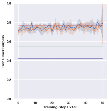
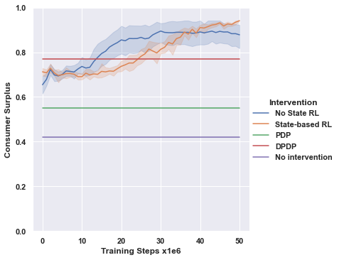
Figure 1: Learning performance of No State RL and State-based RL compared with different baselines. The results are averaged over 10 runs and shaded regions show 95% confidence intervals. The No-Stackelberg interventions are displayed on the left, the Stackelberg ones are on the right.

Figure 1 shows the consumer surplus that is realized under these different interventions. First, we confirm the results of Johnson et al. (2020), and see consumer surplus improvements from both PDP and DPDP compared to No intervention, with DPDP outperforming PDP. At the same time, the no Stackelberg baselines are not able to outperform DPDP, confirming the benefits of using learning methodologies that exploit the leader-follower structure of our game. Indeed, our RL interventions based on the Stackelberg framework dramatically improve consumer surplus, driving it close to its maximal level, which is slightly above 0.94. This is confirmed by the fact that, for both No State and State-based RL, all sellers are displayed and they invariably quote minimum prices at the end of training. This is the optimal (i.e., surplus maximizing) seller behavior, confirming the effectiveness of the Stackelberg-based learning methodology in finding an optimal leader strategy given the Q-learning behavior of sellers.

5.2 Learning in the Wild

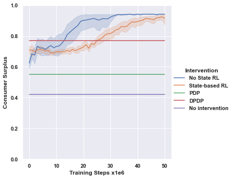
Figure 2: Offline learning (left) vs. online, “learning in the wild” (right) performance. The results are averaged over 10 runs, and the shaded regions show 95% confidence intervals.

We now test the performance of the Stackelberg POMDP learning methodology when it has no access to sellers’ private information during training. This can potentially create learning instabilities given that actor-critic training such as A2C generally require that the environment accessed by their critic networks is Markovian (Grondman et al., 2012). Despite this, we find success in this test of “in the wild” learning. The results are displayed in Figure 2 and show that, despite relaxing this Markov assumption, the A2C algorithm is able to learn optimal policies for both policy classes (No State and State-based). For No State RL this comes along with lower variance. For State-based RL, the empirical performance is roughly unaffected. We conjecture that the reason behind this good performance is related to the class of threshold platform policies. Given a threshold policy, it is possible to predict the overall episode reward based only on the action taken by the policy (the threshold) and ignoring the part of the state that is internal to the sellers (i.e., the Q-matrix and exploration rate). Thus, we see empirically that the additional information that relates to sellers’ learning can actually make the platform’s learning problem harder.

In Appendix E, we also demonstrate successful experimental results when we replace the use of consumer surplus (1) for reward with a reward that corresponds to the number of agents displayed and the sum of the negated prices offered by sellers. This shows robustness to a possible knowledge gap in knowing the specific functional form of consumer surplus.

5.3 Robustness of Learned Platform Rules

As observed in our previous experiments, the Stackelberg-based RL algorithm is effective in learning interventions that maximize consumer surplus for a given economic setting. However, as they are tailored to the economic setting at hand, these interventions can perform poorly when facing settings that are different from those during training. To learn more robust platform rules, we also train with a modified version of the Stackelberg POMDP: at each reward step, with some random-price probability, sellers quote prices sampled uniformly at random from the price grid. In this way, the platform is rewarded during training for performance that remains robust to prices that are not produced by the Q-learning equilibrium dynamics (given seller costs at training).

We evaluate the effect of adding this perturbation-based robustness to the training procedure in settings with different seller costs: in addition to the default $c=1.0$, we also test with cost $c=1.38$ (between the second and the third price in our price grid) and cost $c=1.67$ (between the third and the fourth price in the price grid). Here, and for additional realism, we also continue to train the platform rule according to the “in the wild” approach described above, in Section 5.2.

As we see in Figure 3, this training approach (and in particular with probability 0.4 of random-price perturbation) succeeds in making the state-based policy much more robust in the face of sellers who experience a different cost environment at test time. The robust, state-based policy displays sellers with higher prices (due to their higher costs), while continuing to significantly mitigate collusion when seller costs are as they were during training. This is also confirmed by the policy visualizations in Figure 4, which show how the buy box learned for State-based RL tends to be much more open under this modified training regime. In contrast, the policy learned by No State RL performs very poorly (zero consumer surplus) when tested at costs that differ from those assumed during training, and even under this modified training regime. There is no single threshold that provides a good compromise between performance at cost $1$ and handling price perturbations.

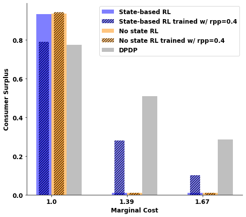
Figure 3: Robustness test, with buy box policy trained without price perturbation and with price perturbation with prob. 0.4, averaged over 10 runs.

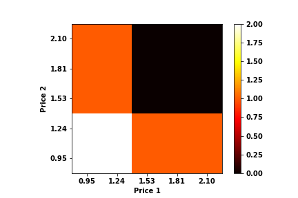
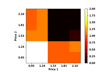
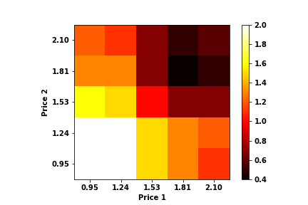
Figure 4: Policy visualization - number of displayed agents given price selection, averaged over 10 seeds (white–avg. num. sellers displayed 2, black–avg. num. sellers displayed 0). (Top-left): No state RL with no price perturbation in the reward step. (Top-right): No state RL with 40% random price probability in the reward step. (Bottom-left): State-based RL with no price perturbation in the reward step. (Bottom-right): State-based RL with 40% random price probability in the reward step.

6 Conclusion

This work has demonstrated that rules that are effective in preventing collusion by sellers can be learned through a framework that correctly solves the two-level, Stackelberg problem (making use of the platform’s commitment power). Specifically, we have introduced the class of threshold policies that contain policies that optimize consumer surplus and a learning methodology that is effective in learning optimal leader policies in this class. The interventions we learned are shown to substantially outperform the hand-designed interventions introduced in prior work when the cost environment at test time is as anticipated during training. We also showed how our learned platform interventions can be made more robust when settings are dynamic, with varying seller cost structures, by adopting a suitably-modified training methodology. This also highlights the importance of the state-based platform rule relative to a no-state rule.

Interesting future directions include testing our approach in more complex settings, e.g., when sellers’ costs vary between training episodes. In this case, optimal policy actions are based on the prices quoted during the sellers’ equilibration phase, as these prices may provide useful information about the current underlying costs (intuitively, the quoted prices will be higher under higher costs). In this scenario, it may be necessary to represent our platform policies via a recurrent neural network, keeping a memory of past prices. Finally, we believe that this approach can also be effective in other applications, e.g., to design and understand effective interventions for the electricity markets studied by Abada and Lambin (2020), a setting where the successful use of RL as a defensive response by a platform is not yet established.

Appendix A Q Learning

Q learning is an RL algorithm that learns an estimate of the action-value function $Q^{*}(s,a)$. This action-value function gives the expected total reward of taking action $a$ at state $s$ and using the optimal policy function in the future. Once $Q^{*}(s,a)$ has been learned, the optimal policy is

$$\pi^{*}(s)\in\text{arg max}_{a\in A}Q^{*}(s,a).$$ (3)

A Q-learning algorithm maintains an $|S|\times|A|$ Q-matrix, $Q_{t}$, representing the estimate of $Q^{*}(s,a)$ at step $t$. Usually, this matrix is randomly initialized. At each step $t$, the algorithm takes action $a_{t}$ that with probability $1-\varepsilon_{t}$ is optimal according to its current Q-matrix $Q_{t}$, and with probability $\varepsilon_{t}$ chosen uniformly at random from the set of avalilable actions. We call $\varepsilon_{t}$ the exploration rate. The entry $(s_{t},a_{t})$ of $Q_{t}$ is updated based on feedback via a convex combination of its previous value and the reward $r(s_{t},a_{t})$ attained from the action plus the discounted value of the state $s_{t+1}$:

$$Q_{t+1}(s_{t},a_{t})=(1-\alpha)Q_{t}(s_{t},a_{t})+\alpha[r(s_{t},a_{t})+\delta\max_{a\in A}Q_{t}(s_{t+1},a)].$$ (4)

Parameter $\alpha\in[0,1]$ is the learning rate. When the environment is stationary and Markovian, and under suitable assumptions on the learning rate and exploration rate, the Q-matrix is guaranteed to converge in the limit to the action-value function $Q^{*}(s,a)$ and the policy to the optimal policy.

Appendix B Variations on Setting Parameters

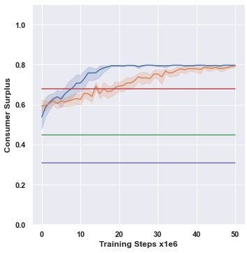
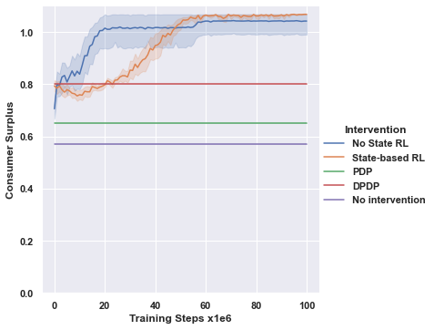
Figure 5: “Learning in the wild” performance of No State RL and State-based RL with different environment settings when (left) the horizontal differentiation $\mu$ is lowered from 0.25 to 0.05, and when (right) $\mu$ is increased from 0.25 to 0.40. The results are averaged over 10 runs, and the shaded regions show 95% confidence intervals.

Following Calvano et al. (2020a) and Johnson et al. (2020), we also consider the learning performance of our RL algorithms in settings with different horizontal differentiation parameter $\mu$. Specifically, Figure 5 displays our training curves when the horizontal differentiation is lowered from 0.25 to 0.05 and increased from 0.25 to 0.40, and our policies are learned “in the wild.” We notice that, in both scenarios, our RL policies bring consumer welfare close to its optimal level (0.8 when $\mu=0.05$ and 1.08 when $\mu=0.4$) outperforming all the baselines.

Appendix C Deterministic Policies During Stackelberg POMDP Episodes

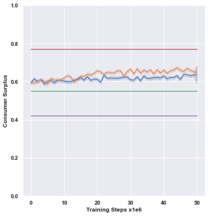
Figure 6: “Learning in the wild” performance of No State RL and State-based RL when policies are non-deterministic (left) and deterministic (right) during Stackelberg POMDP episodes. The results are averaged over 10 runs and shaded regions show 95% confidence intervals.

In this section, we test the learning performance of our RL algorithms when policies are not deterministic during the Stackelberg POMDP episodes. As we can see from Figure 6, this variation dramatically affects our learning performance, which only slightly improves during training and leads to final policies that do not outperform our baselines. As discussed in Section 5, this poor performance is caused by the sellers not being able to learn optimal response strategies due to the high variance introduced by the non-deterministic behavior of our policies.

Appendix D Variations on Sellers’ Learning Behavior

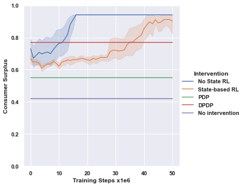
Figure 7: “Learning in the wild” performance of No State RL and State-based RL when sellers restart their exploration asynchronously during Stackelberg POMDP episodes. The results are averaged over 10 runs and shaded regions show 95% confidence intervals.

In our previous experiments, we assumed that both sellers restart their learning processes any time the platform rules change. This is consistent with the original experiments run by Calvano et al. (2020a), which demonstrated seller collusive behavior. However, this assumption may not hold in real-world settings, where sellers can restart their learning processes asynchronously and at any time. This behavior can present new challenges to learning an effective platform policy. Indeed, in this scenario, changes in the sellers’ behavior may be caused not only by different platform interventions, but also as a result of learning restarts.

In this section, we evaluate the performance of the Stackelberg POMDP framework in scenarios where sellers randomly restart their exploration rate during training. Specifically, we assume that, at each step of the platform’s learning process, each seller restarts its exploration rate with some probability. We set this probability such that, in expectation, each seller restarts its exploration once per Stackelberg POMDP episode (which corresponds to the number of steps between platform updates). A particular concern is that this behavior may result in effectively random prices if a restart occurs close to the nominal reward phase of the Stackelberg POMDP episode. A sensible response of a platform to this would be to monitor sellers’ prices, and isolate stages when price profiles are more stable to audit rewards. For a stylized version of this, we allow sellers’ exploration to restart as outlined above, but pause any exploration during the reward phase of the Stackelberg POMDP. Furthermore, if restarts occur close to the reward phases, rewards may reflect an out-of-equilibrium behavior of the sellers (even if exploration is paused). To avoid this problem, we generate our plots by logging rewards in an evaluation Stackelberg POMDP episode we run every 100k training steps. These evaluation episodes use the current platform policy and operate it executing the action with the highest weight given each observation. In these episodes, the Q learning processes are run as in the previous sections, without intra-episode restarts.

As we can see from Figure 7, the Stackelberg learning framework allows us to derive close-to-optimal policies even under this less stationary behavior. Given that rewards are collected in evaluation episodes (where policies are operated via highest-weighted actions), the optimal intervention under No State RL is executed much earlier than in the simulations of Figure 2, reaching the maximum reward after only 15M training steps.

Appendix E Variations on Policy Rewards

In our main experiments, we assume that the platform can compute the consumer surplus $U(p_{t};\mathcal{N}_{t})=\mu\cdot\log[\lambda(p_{t};\mathcal{N}_{t})]$, where $\lambda(p_{t};\mathcal{N}_{t})=\sum_{j\in\mathcal{N}_{t}}\mathrm{exp}((\alpha_{j}-p_{j,t})/\mu)+\mathrm{exp}(\alpha_{0}/\mu)$ at each step $t$ to reward the policy. We note that, however, to compute this surplus one needs to access the consumers’ quality indexes $\alpha_{i}$s, which may not be available to the platform. However, we note that, to maximize consumer surplus, we can replace $U(p_{t};\mathcal{N}_{t})$ with any reward function that increases with respect to the number of agents displayed and decreases as prices increase. In this section, we will use $\tilde{U}(p_{t};\mathcal{N}_{t})=\mu\cdot\log[\tilde{\lambda}(p_{t};\mathcal{N}_{t})]$, where $\tilde{\lambda}(p_{t};\mathcal{N}_{t})=\sum_{j\in\mathcal{N}_{t}}\mathrm{exp}(-p_{j,t}/\mu)$. As we can see from Figure 8, our Stackelberg training framework can derive optimal policies even under these modified rewards.

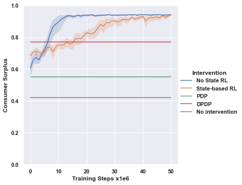
Figure 8: Learning performance under reward that does not access quality indexes.

References

- (1)
- Abada and Lambin (2020) Ibrahim Abada and Xavier Lambin. 2020. Artificial Intelligence: Can Seemingly Collusive Outcomes Be Avoided? Available at SSRN 3559308 (2020).
- Anderson and De Palma (1992) Simon P Anderson and Andre De Palma. 1992. The logit as a model of product differentiation. Oxford Economic Papers 44, 1 (1992), 51–67.
- Areyan Viqueira et al. (2019) Enrique Areyan Viqueira, Cyrus Cousins, Yasser Mohammad, and Amy Greenwald. 2019. Empirical Mechanism Design: Designing Mechanisms from Data. In Proceedings of the Thirty-Fifth Conference on Uncertainty in Artificial Intelligence (Proceedings of Machine Learning Research, Vol. 115). 1094–1104.
- Assad et al. (2020) Stephanie Assad, Robert Clark, Daniel Ershov, and Lei Xu. 2020. Algorithmic Pricing and Competition: Empirical Evidence from the German Retail Gasoline Market. CESifo Working Paper Series 8521 (2020).
- Boutilier (1996) Craig Boutilier. 1996. Planning, Learning and Coordination in Multiagent Decision Processes. In Proceedings of the 6th Conference on Theoretical Aspects of Rationality and Knowledge. 195–210.
- Brero et al. (2021a) Gianluca Brero, Darshan Chakrabarti, Alon Eden, Matthias Gerstgrasser, Vincent Li, and David Parkes. 2021a. Learning Stackelberg Equilibria in Sequential Price Mechanisms. In ICML Workshop for Reinforcement Learning Theory.
- Brero et al. (2021b) Gianluca Brero, Alon Eden, Matthias Gerstgrasser, David C. Parkes, and Duncan Rheingans-Yoo. 2021b. Reinforcement Learning of Sequential Price Mechanisms. In Thirty-Fifth AAAI Conference on Artificial Intelligence, AAAI. 5219–5227.
- Brinkman and Wellman (2017) Erik Brinkman and Michael P. Wellman. 2017. Empirical Mechanism Design for Optimizing Clearing Interval in Frequent Call Markets. In Proceedings of the 2017 ACM Conference on Economics and Computation. 205–221.
- Bünz et al. (2018) Benedikt Bünz, Benjamin Lubin, and Sven Seuken. 2018. Designing Core-selecting Payment Rules: A Computational Search Approach. In Proceedings of the 2018 ACM Conference on Economics and Computation. 109.
- Calvano et al. (2020b) Emilio Calvano, Giacomo Calzolari, Vincenzo Denicolò, Joseph E Harrington, and Sergio Pastorello. 2020b. Protecting consumers from collusive prices due to AI. Science 370, 6520 (2020), 1040–1042.
- Calvano et al. (2020a) Emilio Calvano, Giacomo Calzolari, Vincenzo Denicolo, and Sergio Pastorello. 2020a. Artificial intelligence, algorithmic pricing, and collusion. American Economic Review 110, 10 (2020), 3267–97.
- Cheng et al. (2017) C. Cheng, Z. Zhu, B. Xin, and C Chen. 2017. A multi-agent reinforcement learning algorithm based on Stackelberg game. In 6th Data Driven Control and Learning Systems (DDCLS). 727–732.
- Curry et al. (2020) Michael J. Curry, Ping-Yeh Chiang, Tom Goldstein, and John Dickerson. 2020. Certifying Strategyproof Auction Networks. In Proc. 33rd Annual Conference on Neural Information Processing Systems.
- Curry et al. (2022) Michael J. Curry, Uro Lyi, Tom Goldstein, and John Dickerson. 2022. Learning Revenue-Maximizing Auctions With Differentiable Matching. In Proc. 25th International Conference on Artificial Intelligence and Statistics. Forthcoming.
- Duetting et al. (2019) Paul Duetting, Zhe Feng, Harikrishna Narasimhan, David C. Parkes, and Sai Srivatsa Ravindranath. 2019. Optimal Auctions through Deep Learning. In Proceedings of the 36th International Conference on Machine Learning. 1706–1715.
- Fiez et al. (2020) Tanner Fiez, Benjamin Chasnov, and Lillian J. Ratliff. 2020. Implicit Learning Dynamics in Stackelberg Games: Equilibria Characterization, Convergence Analysis, and Empirical Study. In Proceedings of the 37th International Conference on Machine Learning. 3133–3144.
- Fudenberg and Tirole (1991) Drew Fudenberg and Jean Tirole. 1991. Game theory. MIT press.
- Fujimoto et al. (2022) Scott Fujimoto, David Meger, Doina Precup, Ofir Nachum, and Shixiang Shane Gu. 2022. Why Should I Trust You, Bellman? The Bellman Error is a Poor Replacement for Value Error. arXiv preprint arXiv:2201.12417 (2022).
- Grondman et al. (2012) Ivo Grondman, Lucian Busoniu, Gabriel AD Lopes, and Robert Babuska. 2012. A survey of actor-critic reinforcement learning: Standard and natural policy gradients. IEEE Transactions on Systems, Man, and Cybernetics, Part C (Applications and Reviews) 42, 6 (2012), 1291–1307.
- Jin et al. (2020) Chi Jin, Praneeth Netrapalli, and Michael I. Jordan. 2020. What is Local Optimality in Nonconvex-Nonconcave Minimax Optimization?. In Proceedings of the 37th International Conference on Machine Learning, Vol. 119. 4880–4889.
- Johnson et al. (2020) Justin Johnson, Andrew Rhodes, and Matthijs R Wildenbeest. 2020. Platform design when sellers use pricing algorithms. CEPR Discussion Paper No. DP15504 (2020).
- Jordan et al. (2010) Patrick R. Jordan, L. Julian Schvartzman, and Michael P. Wellman. 2010. Strategy exploration in empirical games. In 9th International Conference on Autonomous Agents and Multiagent Systems. 1131–1138.
- Kiekintveld and Wellman (2008) Christopher Kiekintveld and Michael P. Wellman. 2008. Selecting strategies using empirical game models: an experimental analysis of meta-strategies. In 7th International Joint Conference on Autonomous Agents and Multiagent Systems. 1095–1101.
- Kuo et al. (2020) Kevin Kuo, Anthony Ostuni, Elizabeth Horishny, Michael J. Curry, Samuel Dooley, Ping-Yeh Chiang, Tom Goldstein, and John P. Dickerson. 2020. ProportionNet: Balancing Fairness and Revenue for Auction Design with Deep Learning. CoRR abs/2010.06398 (2020).
- Li et al. (2019) Shihui Li, Yi Wu, Xinyue Cui, Honghua Dong, Fei Fang, and Stuart Russell. 2019. Robust Multi-Agent Reinforcement Learning via Minimax Deep Deterministic Policy Gradient. Proceedings of the AAAI Conference on Artificial Intelligence 33 (July 2019), 4213–4220.
- Lowe et al. (2017) Ryan Lowe, Yi I Wu, Aviv Tamar, Jean Harb, OpenAI Pieter Abbeel, and Igor Mordatch. 2017. Multi-agent actor-critic for mixed cooperative-competitive environments. Advances in Neural Information Processing Systems (NeurIPS) 30 (2017).
- Mguni et al. (2019) David Mguni, Joel Jennings, Emilio Sison, Sergio Valcarcel Macua, Sofia Ceppi, and Enrique Munoz de Cote. 2019. Coordinating the Crowd: Inducing Desirable Equilibria in Non-Cooperative Systems. In Proceedings of the 18th International Conference on Autonomous Agents and MultiAgent Systems. 386–394.
- Mishra et al. (2020) Rajesh K. Mishra, Deepanshu Vasal, and Sriram Vishwanath. 2020. Model-free Reinforcement Learning for Stochastic Stackelberg Security Games. In 59th IEEE Conference on Decision and Control. 348–353.
- Peri et al. (2021) Neehar Peri, Michael J. Curry, Samuel Dooley, and John P. Dickerson. 2021. PreferenceNet: Encoding Human Preferences in Auction Design with Deep Learning. In Proceedings of the 35th Conference on Neural Information Processing Systems.
- Raffin et al. (2021) Antonin Raffin, Ashley Hill, Adam Gleave, Anssi Kanervisto, Maximilian Ernestus, and Noah Dormann. 2021. Stable-Baselines3: Reliable Reinforcement Learning Implementations. Journal of Machine Learning Research 22, 268 (2021), 1–8.
- Rahme et al. (2021b) Jad Rahme, Samy Jelassi, Joan Bruna, and S. Matthew Weinberg. 2021b. A Permutation-Equivariant Neural Network Architecture For Auction Design. In Proc. Thirty-Fifth AAAI Conference on Artificial Intelligence. 5664–5672.
- Rahme et al. (2021a) Jad Rahme, Samy Jelassi, and S. Matthew Weinberg. 2021a. Auction Learning as a Two-Player Game. In Proc. 9th International Conference on Learning Representations, ICLR.
- Sengupta and Kambhampati (2020) Sailik Sengupta and Subbarao Kambhampati. 2020. Multi-agent Reinforcement Learning in Bayesian Stackelberg Markov Games for Adaptive Moving Target Defense. arXiv:2007.10457 [cs] (July 2020). arXiv: 2007.10457.
- Shen et al. (2020) Weiran Shen, Binghui Peng, Hanpeng Liu, Michael Zhang, Ruohan Qian, Yan Hong, Zhi Guo, Zongyao Ding, Pengjun Lu, and Pingzhong Tang. 2020. Reinforcement mechanism design: With applications to dynamic pricing in sponsored search auctions. In Proceedings of the AAAI Conference on Artificial Intelligence, Vol. 34. 2236–2243.
- Shen et al. (2019) W. Shen, P. Tang, and S. Zuo. 2019. Automated Mechanism Design via Neural Networks. In Proceedings of the 18th International Conference on Autonomous Agents and Multiagent Systems.
- Shi et al. (2020) Zhenyu Shi, Runsheng Yu, Xinrun Wang, Rundong Wang, Youzhi Zhang, Hanjiang Lai, and Bo An. 2020. Learning Expensive Coordination: An Event-Based Deep RL Approach. In 8th International Conference on Learning Representations.
- Shu and Tian (2019) Tianmin Shu and Yuandong Tian. 2019. M^3RL: Mind-aware Multi-agent Management Reinforcement Learning. In 7th International Conference on Learning Representations.
- Tacchetti et al. (2019) Andrea Tacchetti, DJ Strouse, Marta Garnelo, Thore Graepel, and Yoram Bachrach. 2019. A Neural Architecture for Designing Truthful and Efficient Auctions. CoRR 1907.05181 (2019).
- Tang (2017) Pingzhong Tang. 2017. Reinforcement mechanism design.. In Proc. 26th Int Joint Conf. on Art. Intell. (IJCAI). 5146–5150.
- Tharakunnel and Bhattacharyya (2007) K. Tharakunnel and S. Bhattacharyya. 2007. Leader-follower semi-markov decision problems: theoretical framework and approximate solution. In IEEE International Symposium on Approximate Dynamic Programming and Reinforcement Learning. 111–118.
- The Organisation for Economic Co-operation and Development (2017) The Organisation for Economic Co-operation and Development. 2017. Algorithms and Collusion– Note from the European Union. www.oecd.org/competition/algorithms-and-collusion.htm
- U.S. Federal Trade Commission (2018) U.S. Federal Trade Commission. 2018. The Competition and Consumer Protection Issues of Algorithms, Artificial Intelligence, and Predictive Analytics, Hearing on Competition and Consumer Protection in the 21st Century, U.S. Federal Trade Commission. https://www.ftc.gov/policy/hearings-competition-consumer-protection
- Vorobeychik et al. (2006) Yevgeniy Vorobeychik, Christopher Kiekintveld, and Michael P. Wellman. 2006. Empirical mechanism design: methods, with application to a supply-chain scenario. In Proceedings 7th ACM Conference on Electronic Commerce (EC-2006). 306–315.
- Wang et al. (2022) Kai Wang, Lily Xu, Andrew Perrault, Michael K. Reiter, and Milind Tambe. 2022. Coordinating Followers to Reach Better Equilibria: End-to-End Gradient Descent for Stackelberg Games. In AAAI Conference on Artificial Intelligence.
- Wellman (2006) Michael P. Wellman. 2006. Methods for Empirical Game-Theoretic Analysis. In Proceedings, The Twenty-First National Conference on Artificial Intelligence. 1552–1556.
- Xu et al. (2021) Lily Xu, Andrew Perrault, Fei Fang, Haipeng Chen, and Milind Tambe. 2021. Robust Reinforcement Learning Under Minimax Regret for Green Security. In Proc. 37th Conference on Uncertainty in Artifical Intelligence (UAI-21).
- Zheng et al. (2022) Stephan Zheng, Alexander Trott, Sunil Srinivasa, David C Parkes, and Richard Socher. 2022. The AI Economist: Optimal Economic Policy Design via Two-level Deep Reinforcement Learning. Science Advances 8 (2022).