Coalescent point process of branching trees in varying environment

Abstract

Consider an arbitrary large population at the present time, originated at an unspecified arbitrary large time in the past, where individuals in the same generation reproduce independently, forward in time, with the same offspring distribution but potentially changing among generations. The genealogy of the current generation backwards in time is uniquely determined by the coalescent point process $(A_{i},i\geq 1)$, where $A_{i}$ is the coalescent time between individuals $i$ and $i+1$. In general, this process is not Markov. In constant environment, Lambert and Popovic (2013) proposed a Markov process of point measures to reconstruct the coalescent point process. We present a counterexample where we show that their process does not have the Markov property. The main contribution of this work is to propose a vector valued Markov process $(B_{i},i\geq 1)$, that reach the goal to reconstruct the genealogy, with finite information for every $i$. Additionally, when the offspring distributions are lineal fractional, we show that the variables $(A_{i},i\geq 1)$ are independent and identically distributed.

Keywords: Branching process in varying environment; Genealogical tree; Coalescent point process; Linear fractional distribution; stopping lines.
MSC2020 subject classifications: 60J80; 60J10; 60J85; 92D25.

1 Introduction

Lambert and Popovic [6] studied the backward genealogy of a random population when the forward time dynamics are produced by a branching process, either discrete or continuous-state space. They were interested in having an arbitrarily large population at the present time, originated at an unspecified arbitrarily large time in the past. For the discrete state case, they used a monotone planar embedding tree where the lines of descent do not intersect. The $i$-th individual in the past $n$-th generation, is represented by $(n,i)$ for any $n\in\mathbb{Z}_{-}:=\{0,-1,-2,\dots\}$ and $i\in\mathbb{N}:=\{1,2,\dots\}$. Individuals at the present generation are simply denoted by $i$ instead of $(0,i)$.

They showed that the genealogy of the current generation backwards in time is uniquely determined by the so-called coalescent point process, $(A_{i},i\geq 1)$, where $A_{i}$ is the coalescent time between individuals $i$ and $i+1$. In general, this process is not Markov and its law is difficult to characterize. To solve this problem, they constructed a sequence valued process $(D_{i},i\geq 1)$ such that for every $i$, $A_{i}$ is the first non-zero entry of $D_{i}$. This process is Markov but for every $i$, $D_{i}$ and $D_{i+1}$ are the same infinite sequence, except for a finite number of entries. Hence, $(D_{i},i\geq 1)$ has a lot repetitive information. Therefore, they constructed a process $(\widetilde{B}_{i},i\geq 1)$ by removing some information from $(D_{i},i\geq 1)$. They claimed that $(\widetilde{B}_{i},i\geq 1)$ contains the minimal amount of information needed to construct $(A_{i},i\geq 1)$ while remaining Markov. However, they did a mistake in their proof and as you can see in Example 3.1, $(\widetilde{B}_{i},i\geq 1)$ is not always Markov.

In this paper, we aim to define a coalescent point process for a population driven by a Galton-Watson process in varying environment, that is, individuals in the same generation have the same offspring distribution but these distributions vary along the generations. Our main contribution is to propose a new Markov process $(B_{i},i\geq 0)$ that reach the goal to reconstruct the genealogy of a population in varying environment, with finite information for every $i$. This property plays an important role. The reason comes from real life applications, where evolutionary biologists are interested in reconstruct the genealogy of a population, based on a sample with finite number of individuals. Therefore, we can not use the process $(D_{i},i\geq 1)$ as a model, because $(D_{i},i\geq 1)$ required a infinite sequence of values. In the constant environment case, this process corrects the mistake done by Lambert and Popovic [6], when they try to construct a Markovian process with less (finite quantity) information than $(D_{i},i\geq 1)$.

We use the same planar embedding as [6] and propose a vector-valued process $(B_{i},i\geq 0)$ constructed in the following recursive way. We define $B_{0}=\emptyset$, the empty vector. For any fixed individual $i$, we follow its ancestral line (the so called spine). For every $n\in\mathbb{N}$, we consider the subtree attached to the spine with root at generation $-n$. We denote by $B_{i}(n)$ the number of children of the root at the right hand side of the spine, whose descendants are alive at the present generation. Then, we define the vector $B_{i}=(B_{i}(1),\dots,B_{i}(l_{i}))$, where its length $l_{i}$ is the maximum between $l_{i-1}$ and the first $n$ such that $B_{i}(n)\neq 0$. By construction, $A_{i}$ is the first non-zero entry of $B_{i}$. In addition, we can see that $l_{i}$ is the coalescent time between individuals $1,2,\dots,i+1$. See Figure 1.

$i$	$A_{i}$	$B_{i}$
$1$	$1$	$(1)$
$2$	$2$	$(0,2)$
$3$	$1$	$(1,1)$
$4$	$2$	$(0,1)$
$5$	$1$	$(2,0)$
$6$	$1$	$(1,0)$
$7$	$4$	$(0,0,0,1)$
$8$	$3$	$(0,0,1,0)$
$9$	$5$	$(0,0,0,0,1)$
$10$	$1$	$(1,0,0,1,0)$
$11$	$4$	$(0,0,0,1,0)$

Figure 1: A Galton-Watson tree in varying environment and its processes $(A_{i},i\geq 1)$ and $(B_{i},i\geq 1)$. We use colors to represent the different subtrees with roots in the spine of individual $1$, whose descendants are alive at the present generation. The length of the vector $B_{i}$ is the height of the subtree attached to the first spine that contains individual $i+1$.

If the environment is constant, Lambert and Popovic [6] showed that the process $(A_{i},i\geq 1)$ is Markov only when the offspring distribution is linear fractional. If the environment is not constant but still linear fractional, we show in Proposition 3.4 that $(A_{i},i\geq 1)$ is Markov. Moreover, it is a sequence of independent and identically distributed random variables and we obtain its distribution.

The remainder of the paper is structured as follows. In Section 2, we present Galton-Watson processes in varying environment and some related properties. In particular, for the associated tree, we development the concept of stopping lines, as an analogy to stopping times, to get a general branching property. The definitions of $(A_{i},i\geq 1)$ and $(B_{i},i\geq 1)$ are given in Section 3. In the same section, we present our main theorem: $(B_{i},i\geq 1)$ is a Markov process which has finite information for every $i$ and reconstruct $(A_{i},i\geq 1)$. In addition, if the offspring distributions are linear fractional we show that the process $(A_{i},i\geq 1)$ is Markov and we give explicitly its distribution. Finally, Section 4 is devoted to the proofs.

2 Galton-Watson processes in varying environment

Galton-Watson processes in varying environment model the development of the size of a population, where individuals reproduce independently with offspring distribution potentially changing among generations. To be precise, a varying environment is a sequence $\mathcal{E}=(e_{n},n\geq 1)$ of probability measures on $\mathbb{N}_{0}:=\{0,1,\dots\}$. Let $Z_{n}$ be the population size at generation $n$. The process $(Z_{n},n\geq 0)$ is a Markov chain defined recursively as

$$Z_{0}=1\qquad\mbox{and}\qquad Z_{n+1}=\sum_{i=1}^{Z_{n}}\xi_{i}^{(n)},\quad n\geq 0,$$

where $\xi_{i}^{(n)}$ denotes the offspring of the $i$-th individual living at generation $n$ and it has distribution $e_{n+1}$. We assume that the variables $(\xi^{(n)}_{i},i\geq 1,n\geq 1)$ are all independent. The process $\{(Z_{n},n\geq 0);\mathbb{P}\}$ is called a Galton Watson process in varying environment $\mathcal{E}$, for short GWVE.

Let $f_{n}$ be the generating function of $e_{n}$. For each $0\leq m<n$ and $s\in[0,1]$, we define

$$f_{m,n}(s):=f_{m+1}\circ\cdots\circ f_{n}(s),\qquad\mbox{and}\qquad\qquad f_{n,n}(s):=s,$$ (1)

where $\circ$ denotes the composition. Note that for every $s\in[0,1]$ and $0\leq m<n$,

$$f^{\prime}_{m,n}(s)=\prod_{\ell=m+1}^{n}f^{\prime}_{\ell}(f_{\ell,n}(s)),\qquad\mbox{and}\qquad f^{\prime}_{n,n}(s)=1.$$ (2)

Let $k\geq 0$, according to Kersting and Vatutin [3], we have

$$\mathbb{E}(s^{Z_{k+n}}\mid Z_{k}=1)=f_{k,k+n}(s),\qquad 0\leq s\leq 1,\quad n\geq 0.$$

In particular, $(Z_{k+n},n\geq 0)$ conditionally on $\{Z_{k}=1\}$, has the same law as a Galton Watson process in varying environment $\,\mathcal{E}^{(k)}:=(e_{k+n},n\geq 1)$. For a short notation, we denote by $\{(Z_{n},n\geq 0);\mathbb{P}^{(k)}\}$ the law of the process with the shifted environment $\,\mathcal{E}^{(k)}$.

A Galton Watson tree in varying environment $\mathcal{E}$, for short GWVE tree, is the genealogical tree associated with $\{(Z_{n},n\geq 0);\mathbb{P}\}$ starting with one individual. It can be view as a planar rooted tree $T$, with edges connecting parents to children, and the root as the initial individual. Any individual that appears in the tree may be labeled through its ancestry using the Ulam-Harris notation. For example: an individual $x=(x_{1},\dots,x_{n-1},x_{n})\in T$ is the $x_{n}$-th child of the $x_{n-1}$-th child of $\dots$ of the $x_{1}$-th child of the root, $\emptyset$. In this way we understand that the length or generation in which $x$ resides is $|x|=n$. For $x=(x_{1},\dots,x_{n})$ and $y=(y_{1},\dots,y_{m})$, we denote by $xy=(x_{1},\dots,x_{n},y_{1},\dots,y_{m})$ the concatenation of $x$ and $y$, with the convention that $x\emptyset=\emptyset x=x$. For $x,y\in T$, we say that $y$ is an ancestor of $x$ (or $x$ is a descendant of $y$) if there exists a $w\in\{\emptyset\}\bigcup\bigcup_{n\geq 1}\mathbb{N}^{n}$ such that $x=yw$. This is usually written by $y\preceq x$ (or $x\succeq y$). Observe that $x\preceq x$.

For $x\in T$, let $T^{(x)}$ be the subtree with root in $x$. Note that $T^{(x)}$ is the genealogical tree associated with $\{(Z_{n},n\geq 0);\mathbb{P}^{(\mid x\mid)}\}$ starting with one individual. By the branching property, it is well know that conditionally on the number of individuals in a given generation, the subtrees with root in that generation are independent. In Proposition 2.1, we develop a stronger property. For this, we present some concepts, early introduced in [1] and later used by [4], [5]. A line $L$ is a family of vertices in $T$, such that every branch started at the root contains at most one vertex in $L$. Hence, for two distinct vertices in the line, neither one is a descendant of the other. Associated with a line $L$ is its $\sigma$-algebra $\mathcal{F}_{L}:=\sigma(\Omega_{x}:x\notin\mathfrak{D}_{L})$, where $\mathfrak{D}_{L}:=\{y\in T:\exists x\in L\mbox{ with }x\preceq y\}$; and for each $x\in T$, $\Omega_{x}$ is the information about the number of children of $x$ together with the edges connecting $x$ with its children. Let $\mathcal{G}_{x}=\sigma(\Omega_{y}:y\preceq x)$. A stopping line $L$ is a random line such that $\{x\in L\}\in\mathcal{G}_{x}$, for every $x\in T$. For instance, $L=\{x\}$ is a stopping line for every $x\in T$.

Proposition 2.1.

Let $L$ be a stopping line for a GWVE tree associated with the process $\{(Z_{n},n\geq 0);\mathbb{P}\}$. Conditioned on $\mathcal{F}_{L}$, the subtrees $\{T^{(x)}:x\in L\}$ are independent. Moreover, for each $x\in L$, the tree $T^{(x)}$ conditioned on $\mathcal{F}_{L}$ has the same law as the genealogical tree associated with $\{(Z_{n},n\geq 0);\mathbb{P}^{(\mid x\mid)}\}$. In other words,

$$\mathbb{E}\left(\prod_{x\in L}\varphi_{x}(T^{(x)})\Big{|}\mathcal{F}_{L}\right)=\prod_{x\in L}\mathbb{E}^{(\mid x\mid)}\left(\varphi_{x}(T)\right),$$

where $(\varphi_{x},x\in L)$ are non-negative measurable functions on the space of planar rooted trees.

Proof.

By the Monotone Class Theorem for functions, it is enough to work with $\varphi_{x}=\mathbb{1}_{A_{x}}$ for some measurable subsets $A_{x}$. Assume that $L=\{x_{1},\dots,x_{n}\}$ is a stopping line. Then, $x_{i}$ is neither ancestor or descendant of $x_{1}$, for $i\geq 2$. Therefore $T^{(x_{i})}\in\mathcal{F}_{x_{1}}$ for $i\geq 2$. Since $\mathcal{F}_{L}\subset\mathcal{F}_{x_{1}}$, by the tower property

$$\mathbb{E}\left(\prod_{i=1}^{n}\mathbb{1}_{A_{i}}(T^{(x_{i})})\Big{|}\mathcal{F}_{L}\right) =\mathbb{E}\left(\mathbb{E}\left(\prod_{i=1}^{n}\mathbb{1}_{A_{i}}(T^{(x_{i})})\Big{|}\mathcal{F}_{x_{1}}\right)\Big{|}\mathcal{F}_{L}\right)$$

$$=\mathbb{E}\left(\prod_{i=2}^{n}\mathbb{1}_{A_{i}}(T^{(x_{i})})\mathbb{E}\left(\mathbb{1}_{A_{1}}(T^{(x_{1})})\Big{|}\mathcal{F}_{x_{1}}\right)\Big{|}\mathcal{F}_{L}\right)$$

$$=\mathbb{E}^{(\mid x_{1}\mid)}\left(\mathbb{1}_{A_{1}}(T^{(x_{1})})\right)\mathbb{E}\left(\prod_{i=2}^{n}\mathbb{1}_{A_{i}}(T^{(x_{i})})\Big{|}\mathcal{F}_{L}\right).$$

In the last equality we have used that $T^{(x_{1})}$ is the genealogical tree associated with $\{(Z_{n},n\geq 0);\mathbb{P}^{(\mid x_{1}\mid)}\}$ and the branching property. Repeating the argument, we conclude the finite case. The general result follows from considerations of a sequence of finite $L_{n}\uparrow L$, monotone convergence and backwards martingale convergence applied to the conditional expectations given $\mathcal{F}_{L_{n}}$, when $\mathcal{F}_{L_{n}}\downarrow\mathcal{F}_{L}$. ∎

We are also interested in the law of the children of the root conditioned to have alive descendants at a fixed generation. Observe that the survival probability up to generation $n$ is

$$\mathbb{P}(Z_{n}>0)=1-f_{0,n}(0).$$ (3)

For $Z_{0}=1$, we define $\zeta_{n}$ as the number of individuals at generation one having alive descendants at generation $n$. In particular, $\zeta_{n}$ has the law of

$$\sum_{i=1}^{\xi^{(0)}}\varepsilon_{i}^{(n)},$$ (4)

where $\xi^{(0)}$ has distribution $e_{1}$ and $(\varepsilon_{i}^{(n)},i\geq 1)$ is a sequence of independent Bernoulli random variables with parameter $1-f_{1,n}(0)$, independent of $\xi^{(0)}$. We also define $\eta_{n}$ as $\zeta_{n}-1$ conditioned on $\{\zeta_{n}\geq 1\}$. Note that the events $\{Z_{n}>0\}$ and $\{\zeta_{n}\geq 1\}$ are equivalent. Moreover, conditionally on $\{Z_{n}>0\}$, there exists an individual at generation $1$ with alive descendants at generation $n$. Therefore, the random variable $\eta_{n}$ can be interpreted as the number of individuals at generation one, having alive descendants at generation $n$ which are different from that individual. Note that for every $k\geq 0$,

$$\mathbb{P}(\eta_{n}=k)=\mathbb{P}(\zeta_{n}=k+1\mid\zeta_{n}\geq 1)=\frac{(1-f_{1,n}(0))^{k+1}f_{1}^{(k+1)}(f_{1,n}(0))}{(k+1)!(1-f_{0,n}(0))},$$ (5)

where $f^{(k+1)}_{1}$ denotes the $(k+1)$-th derivative of $f_{1}$. Indeed, we use

$$\mathbb{E}\left(\xi^{(0)}(\xi^{(0)}-1)\cdots(\xi^{(0)}-k)s^{\xi^{(0)}-k+1}\right)=f^{(k)}_{1}(s)$$

to obtain

$$\mathbb{P}(\zeta_{n}=k+1) =\sum_{i=1}^{\infty}\mathbb{P}(\zeta_{n}=k+1\mid\xi^{(0)}=i)\mathbb{P}(\xi^{(0)}=i)$$

$$=\sum_{i=1}^{\infty}\binom{i}{k+1}(1-f_{1,n}(0))^{k+1}(f_{1,n}(0))^{i-k-1}\mathbb{P}(\xi^{(0)}=i)$$

$$=\frac{(1-f_{1,n}(0))^{k+1}}{(k+1)!}f_{1}^{(k+1)}(f_{1,n}(0)).$$

Similarly,

$$\mathbb{P}(\zeta_{n}=0) =\sum_{i=0}^{\infty}(f_{1,n}(0))^{i}q_{1}(i)=f_{1}(f_{1,n}(0))=f_{0,n}(0).$$

We complete the section with an example where we compute the previous distribution when the offspring distributions are linear fractional.

Example 2.2.

An offspring distribution $\xi$ that satisfies

$$\mathbb{P}(\xi=0)=1-r\qquad\mbox{and}\qquad\mathbb{P}(\xi=k)=rpq^{k-1},\quad k\neq 0,$$

where $0<q<1$, $p=1-q$ and $0\leq r\leq 1$, is called linear fractional. Special cases are $r=1$, where we obtain a geometric distribution $G$; and $r=0$, where we obtain a Dirac measure $\delta_{0}$. If $0<r<1$, it is a mixture of both, i.e. $\xi=rG+(1-r)\delta_{0}$. In this case, its generating function is given by

$$f(s)=1-r\frac{1-s}{1-qs},\qquad s\in[0,1].$$

Thanks to the identity

$$\frac{1}{1-f(s)}=\frac{1}{1-f^{\prime}(1)(1-s)}+\frac{f^{\prime\prime}(1)}{2f^{\prime}(1)^{2}},\qquad s\in[0,1],$$

we can see that a linear fractional distribution is characterized by its mean $f^{\prime}(1)=r/p$ and its normalized second factorial moment $f^{\prime\prime}(1)/f^{\prime}(1)^{2}=2q/r$.

We say that a varying environment $\mathcal{E}=(e_{n},n\geq 1)$ is linear fractional if and only if every $f_{n}$ is linear fractional with parameters $r_{n}$ and $p_{n}$. According with [3, Chapter 1], the generating function $f_{m,n}$ is again linear fractional with mean

$$f_{n,n}^{\prime}(1)=1,\qquad f_{m,n}^{\prime}(1)=f_{m+1}^{\prime}(1)\cdots f_{n}^{\prime}(1)=\frac{r_{m+1}\cdots r_{n}}{p_{m+1}\cdots p_{n}},\qquad m<n,$$

and normalized second factorial moment   $f_{n,n}^{\prime\prime}(1)/f_{n,n}^{\prime}(1)^{2}=0$; and for $m<n$,

$$\frac{f_{m,n}^{\prime\prime}(1)}{f_{m,n}^{\prime}(1)^{2}}=\frac{f_{m+1}^{\prime\prime}(1)}{f_{m+1}^{\prime}(1)^{2}}+\underset{k=m+2}{\overset{n}{\sum}}\frac{1}{f_{m+1}^{\prime}(1)\cdots f_{k-1}^{\prime}(1)}\frac{f_{k}^{\prime\prime}(1)}{f_{k}^{\prime}(1)^{2}}=\frac{2q_{m+1}}{r_{m+1}}+\underset{k=m+2}{\overset{n}{\sum}}\frac{2p_{m+1}\cdots p_{k-1}q_{k}}{r_{m+1}\cdots r_{k-1}r_{k}}.$$

Consider a Galton-Watson process $(Z_{n}:n\geq 0)$ with the previous environment. Then, $Z_{n}$ is linear fractional with generating function $f_{0,n}$. Furthermore, by using (5) and

$$f_{1}^{(k+1)}(s)=\frac{(k+1)!r_{1}(1-q_{1})q_{1}^{k}}{(1-q_{1}s)^{k+2}},$$

we can prove that $\eta_{n}$ has geometric distribution. More precisely,

$$\begin{split}\mathbb{P}(\eta_{n}=k)=&\left(\frac{1-q_{1}}{1-q_{1}f_{1,n}(0)}\right)\left(\frac{q_{1}(1-f_{1,n}(0))}{1-q_{1}f_{1,n}(0)}\right)^{k},\qquad k\geq 0.\end{split}$$

In other words, $\mathbb{P}(\eta_{1}=k)=(1-q_{1})q_{1}^{k},$ for $k\geq 0$; and for $n\geq 2$

$$\begin{split}\mathbb{P}(\eta_{n}=k)=&\left(\frac{1+\underset{i=2}{\overset{n}{\sum}}s_{i,n}}{1+\underset{i=1}{\overset{n}{\sum}}s_{i,n}}\right)\left(\frac{s_{1,n}}{1+\underset{i=1}{\overset{n}{\sum}}s_{i,n}}\right)^{k},\qquad k\geq 0,\end{split}$$

where $s_{n,n}=\tfrac{1-p_{n}}{p_{n}}$ and $s_{i,n}=\tfrac{(1-p_{i})}{p_{i}}\tfrac{r_{i+1}\cdots r_{n}}{p_{i+1}\cdots p_{n}}$ for $\,i<n$.

In the next section, we are going to analyze the backward genealogy of a random population when the forward in time dynamics are produced by a Galton-Watson process in varying environment. The offspring distributions will be denoted by $\mathcal{E}=(e_{m},m\in\mathbb{Z}_{-})$. The generating function $f_{m,n}$ in (1) can be extended to include $m\leq n\leq 0$.

3 Main results

Consider an arbitrary large population at the present time, originated at an unspecified arbitrary large time in the past, where individuals in the same generation reproduce independently, forward in time, with the same offspring distribution but potentially changing among generations. We denote by $e_{m+1}$ the offspring distribution of individuals at generation $m$. Observe that for each individual in the past, the forward in time process starting at that individual produces a branching tree in varying environment.

In order to analyze the backward genealogy of the present population, we consider a particular embedding of a branching tree, infinite in the number of generations and infinite in the number of individuals at any generation. This embedding has been used to define the coalescent point process. First, defined by Lambert and Popovic [6] for a Galton Watson process and later extended by Popovic and Rivas [7] to multitype Galton Watson process. In this planar embedding, individuals are located at the points $(m,i)$ of a discrete lattice $\mathbb{Z}\times\mathbb{N}$, where the first coordinate $m$ denotes the generation and the second coordinate $i$ denotes the position of the individual in the planar embedding from left to right. Since we are interested in backward genealogies, we restrict ourselves to $\mathbb{Z}_{-}$, where the present generation is denoted by $m=0$. Each vertex in the lattice is connected to its offspring represented by some vertices in the level above, in such a way that empty spaces and intersections between lineages are avoided. More precisely, let $\xi^{(m)}_{i}$ be the number of offspring of individual $(m,i)$. We endow the population with the following genealogy: individual $(m,i)$ has mother $(m-1,j)$ if and only if

$$\sum_{k=1}^{j-1}\xi_{k}^{(m-1)}<i\leq\sum_{k=1}^{j}\xi_{k}^{(m-1)}.$$

We suppose that the variables $\{\xi^{(m)}_{i},i\geq 1,m\in\mathbb{Z}_{-}\}$ are independent and the sequence $\{\xi^{(m)}_{i},i\geq 1\}$ has common distribution $e_{m+1}$, for every $m\in\mathbb{Z}_{-}$. In the rest of the paper, the varying environment is denote by $\mathcal{E}=(e_{m},m\in\mathbb{Z}_{-})$.

We now continue introducing the elements for recovering the genealogy. For $n\in\mathbb{N}$, let $\mathfrak{a}_{i}(n)$ be the index of the ancestor of individual $i$ in generation $-n$. The coalescent time $C_{i,j}$ of individuals $i$ and $j$ is denoted by

$$C_{i,j}:=\min\{n\geq 1:\mathfrak{a}_{i}(n)=\mathfrak{a}_{j}(n)\},\qquad i,j\in\mathbb{N},$$

with the agreement that $\min\emptyset=\infty$. We define

$$A_{i}:=C_{i,i+1},\qquad i\in\mathbb{N}.$$

By construction, $C_{i,j}=\max\{A_{i},A_{i+1},\dots,A_{j-1}\}$, for any $i<j$. Therefore, $(A_{i},i\geq 1)$ contains all the genealogical information of the current population. The sequence $\mathbf{A}:=(A_{i},i\geq 1)$ is called the coalescent point process in varying environment. This process was first defined in [6], when the forward time dynamics were produced by a branching process in constant environment.

The distribution of $\mathbf{A}$ is not easy to find and in general it is not a Markov process, except for some special cases. Motivated by the constant environment case [6], let us define an auxiliary Markov process that characterize the genealogy. For any fixed individual $i$, we follow its ancestral line (the so called $i$-th spine) and consider the subtrees with roots in this spine. Note that these roots are labeled by $\{(-n,\mathfrak{a}_{i}(n)),n\in\mathbb{N}\}$. At every subtree, we count the number of daughters of the root at the right hand side of the spine, whose descendants are alive at the present generation. To be precise, let

$$\mathcal{D}_{i}(n):=\{\text{daughters of }(-n,\mathfrak{a}_{i}(n))\text{ with descendants in }\{(0,j):j\geq i\}\},\qquad n\geq 1,\ i\geq 1.$$

Define

$$D_{i}(n)=\#\mathcal{D}_{i}(n)-1,\qquad i,n\geq 1.$$

For every $i\geq 1$, we define the sequence $D_{i}:=(D_{i}(n),n\geq 1)$. We settle $D_{0}$ as the null sequence and $A_{0}:=\infty$. It follows from the monotone planar embedding that

$$A_{i}=\min\{n\geq 1:D_{i}(n)\neq 0\},\qquad i\geq 0.$$ (6)

As we will establish in Proposition 3.3, the sequence-valued process ${\mathbf{D}}:=(D_{i},i\geq 0)$ has the Markov property. Nevertheless, it has a lot of repetitive information, since for every $i$, $D_{i}$ and $D_{i+1}$ are the same infinite sequence, except for a finite number of entries. In order to not carry on this repetitive information, when the environment is constant, a point measure-valued process $(\widetilde{B}_{i},i\geq 0)$ was recursively defined in [6]. Roughly speaking, when $\widetilde{B}_{i}$ has positive measure at $n$, its multiplicity records the number of children of $(-n,\mathfrak{a}_{i}(n))$ at the right-hand side of the $i$-th spine with descendants in individuals $\{(0,j):j\geq i+1\}$. The construction of the process is as follows: $\widetilde{B}_{0}$ is the null measure. $\widetilde{B}_{1}$ has positive mass at position $A_{1}$ and its multiplicity records the number of children of individual $(-A_{1},\mathfrak{a}_{1}(A_{1}))$, with descendants in individuals $\{(0,j):j\geq 2\}$. Recursively, $\widetilde{B}_{i+1}$ is updated from $\widetilde{B}_{i}$ by decreasing by one the mass at position $A_{i}$ (because the $(i+1)$-th spine is part of the children at the right hand side of the $i$-th spine) and possibly by adding a new mass at position $A_{i+1}$ with the respective multiplicity. Formally, for any finite point measure $b=\sum_{n\geq 1}b(n)\delta_{n}$, we define the minimum of its support as

$$\mathfrak{s}(b):=\min\{n\geq 1:b(n)\neq 0\}.$$

In addition, we define $b^{\ast}=b-\delta_{\mathfrak{s}(b)},$ with the convention that $\mathfrak{s}(b)=\infty$ and $b^{\ast}=b$ if $b$ is the null measure. Then, the process $\widetilde{B}_{i}$ is recursively defined as follows

$$\widetilde{B}_{i+1}:=\left\{\begin{array}[]{ll}\widetilde{B}_{i}^{\ast}+D_{i+1}(A_{i+1})\delta_{A_{i+1}}&\ \text{ if }A_{i+1}\neq\mathfrak{s}(\widetilde{B}_{i})\text{ and }A_{i+1}<\mathfrak{s}(\widetilde{B}_{i}^{\ast}),\\ \widetilde{B}_{i}^{\ast}&\ \text{ otherwise.}\end{array}\right.$$

Now, we provide a counterexample to illustrate that $(\widetilde{B}_{i},i\geq 0)$ could be not a Markov process, and in particular, [6, Theorem 2.2] cannot hold.

Example 3.1.

Consider the process $(\widetilde{B}_{i},i\geq 1)$ associated to Figure 1:

$\widetilde{B}_{1}=\delta_{1}$,	$\widetilde{B}_{2}=2\delta_{2}$,	$\widetilde{B}_{3}=\delta_{1}+\delta_{2}$,	$\widetilde{B}_{4}=\delta_{2}$,	$\widetilde{B}_{5}=2\delta_{1}$,	$\widetilde{B}_{6}=\delta_{1}$,
$\widetilde{B}_{7}=\delta_{4}$,	$\widetilde{B}_{8}=\delta_{3}$,	$\widetilde{B}_{9}=\delta_{5}$,	$\widetilde{B}_{10}=\delta_{1}$	and	$\widetilde{B}_{11}=\delta_{4}$.

We show that this process cannot be Markov by exhibiting that the value of $\widetilde{B}_{11}$ depends on both $\widetilde{B}_{9}$ and $\widetilde{B}_{10}$. By the recursive construction, we observe that $\widetilde{B}_{10}=\delta_{1}$ implies that $\widetilde{B}_{11}=\widetilde{B}_{11}(N)\delta_{N}$ for some $N\geq 2$ with $\widetilde{B}_{11}(N)>0$. Besides, from $\widetilde{B}_{9}=\delta_{5}$ we know that individual $(-5,\mathfrak{a}_{9}(5))$ has a unique daughter $u$, at the right hand side of the $9$-th spine, whose descendants are alive at the present generation. Moreover, since $A_{9}=5$ and $A_{10}=1$, we have that $(-5,\mathfrak{a}_{9}(5))=(-5,\mathfrak{a}_{10}(5))=(-5,\mathfrak{a}_{11}(5))$ and $u$ is part of both the $10$-th and $11$-th spine. Therefore, $\widetilde{B}_{11}(5)=0$ and $N$ cannot be 1 or 5. This implies that the value of $\widetilde{B}_{11}$ depends on $\widetilde{B}_{10}$ and additionally on $\widetilde{B}_{9}$. ∎

Next, we turn our attention to the construction of our process $\mathbf{B}=(B_{i},i\geq 0)$. Let $B_{0}=\emptyset$ and $l_{0}=0$. For $i\geq 1$, consider the first generation $l_{i}$ such that an individual in the $i$-th spine is an ancestor of the present generation individuals $1,\dots,i+1$, i.e. $l_{i}:=C_{1,i+1}.$ We define the vector $B_{i}$ as the restriction of $D_{i}$ to the first $l_{i}$ entries, i.e. $B_{i}=(B_{i}(1),B_{i}(2),\dots,B_{i}(l_{i}))$ with

$$B_{i}(k):=D_{i}(k),\qquad 1\leq k\leq l_{i}.$$

See Figure 1. The length $l_{i}$ can be obtained recursively in terms of $D_{i}$ as the maximum between $l_{i-1}$ and the first $n$ such that $D_{i}(n)\neq 0$,

$$l_{i}=l_{i-1}\vee\min\{n\geq 1:D_{i}(n)\neq 0\}=l_{i-1}\vee A_{i}.$$ (7)

The last equality holds by (6). From now on the process $(B_{i},i\geq 0)$ will be called coalescent point process in varying environment.

The principal result of the present work establishes that the process $\mathbf{B}$ is Markov with state space $\mathcal{V}$ given by the set of all the vectors with entries in $\mathbb{N}$, i.e.

$$\mathcal{V}=\bigcup_{m\in\mathbb{N}}\mathbb{N}^{m}$$

with the convention $\mathbb{N}^{0}=\emptyset$. For any $b=(b(1),b(2),\dots,b(m))\in\mathcal{V}$, we denote its length by $l(b)=m$ with the convention $l(\emptyset)=0$. Let $\mathfrak{s}(b)$ be the first non-zero coordinate of $b$ with the convention $\mathfrak{s}(b)=\infty$, if $b$ is a null vector or the empty set. For any $b=(b(1),b(2),\dots,b(m))\in\mathcal{V}$, we define the vector $b^{*}=(b^{*}(1),b^{*}(2),\dots,b^{*}(m))$ where

$$b^{*}(j)=b(j)-\mathbb{1}_{\{j=\mathfrak{s}(b)\}},\qquad j\leq m,$$

with the convention $b^{*}=b$, if $b$ is a null vector or the empty set.

In order to provide the transitions probabilities, we recall that for each $(m,i)\in\mathbb{Z}_{-}\times\mathbb{N}$, the forward in time dynamics starting at individual $(m,i)$ are produced by a branching process in varying environment. More precisely, if $Z^{(m,i)}(k)$ denotes the number of descendants of individual $(m,i)$ at generation $m+k$, then, $(Z^{(m,i)}(k),k\geq 0)$ is a GWVE process with environment $\mathcal{S}_{(m)}:=(e_{m+1},e_{m+2},\dots,e_{0},0,0,\dots)$ starting with one individual. Then, for every $m\in\mathbb{Z}_{-}$, the probability that an individual at generation $m$ has alive descendants at the present generation is $p_{m}=1-f_{m,0}(0)$, see (3). Moreover, if we denote by $\zeta^{(m)}$ the number of its daughters with alive descendants at generation zero, as a consequence of (4) we have

$$\zeta^{(m)}\overset{\mathcal{L}}{=}\underset{i=1}{\overset{Y}{\sum}}\varepsilon_{i},$$

where $Y\sim e_{m+1}$ and the variables $\varepsilon_{i}$ are Bernoulli with parameter $1-f_{m+1,0}(0)$, all independent. We also define $\eta^{(m)}$ as

$$\eta^{(m)}=\zeta^{(m)}-1,\qquad\mbox{ conditioned on }\{\zeta^{(m)}>0\}.$$ (8)

In particular, by (5)

$$\mathbb{P}(\eta^{(m)}=0)=\frac{(1-f_{m+1,0}(0))f_{m+1}^{\prime}(f_{m+1,0}(0))}{1-f_{m,0}(0)}.$$ (9)

Now we are ready to establish the main theorem, which provides the law of the process $(B_{i},i\geq 0)$. Thanks to (6) and (7), the coalescent time of individuals $i$ and $i+1$ is a functional of $B_{i}$

$$A_{i}=\min\{1\leq n\leq l_{i}:B_{i}(n)\neq 0\},\qquad i\geq 1.$$ (10)

Theorem 3.2.

The vector-valued process $\mathbf{B}=(B_{i},i\geq 0)$ is a Markov chain starting at $B_{0}=\emptyset$. Conditionally on $\,\{B_{i}=(b(1),\dots,b(\ell))\}$, the law of $B_{i+1}=(B_{i+1}(1),B_{i+1}(2),\dots,B_{i+1}(l_{i+1}))$ is given by the following transition probabilities

$$B_{i+1}(m):=\left\{\begin{array}[]{ll}\eta^{(-m)}&\text{ if }\,1\leq m<A_{i}\ \text{ or }\ \ell<m\leq l_{i+1}\\ b(m)-1&\text{ if }\,m=A_{i}\\ b(m)&\text{ if }\,A_{i}<m\leq\ell,\end{array}\right.$$

where $(\eta^{(-m)},m\geq 1)$ is a sequence of independent random variables such that for each $m$, the variable $\eta^{(-m)}$ is distributed as (8), and

$$l_{i+1}=\ell\vee\left(\mathbb{1}_{\{\mathfrak{s}(B_{i}^{*})=\infty\}}\min\{k\in\{1,2,\dots,A_{i}-1\}\cup\{\ell+1,\ell+2,\dots\}:\eta^{(-k)}\neq 0\}\right).$$ (11)

Moreover, the law of $A_{1}$ is given by

$$\mathbb{P}(A_{1}>n)=\prod_{i=1}^{n}\mathbb{P}(\eta^{(i)}=0)=\frac{f^{\prime}_{-n,0}(0)}{1-f_{-n,0}(0)}=\mathbb{P}(Z_{n}=1\mid Z_{n}=0),\qquad$$

where $(Z_{k},k\geq 0)$ is a GWVE with environment $\mathcal{S}_{(-n)}$ for every $n\geq 1$.

By similar arguments as in the above theorem, we can obtain the next proposition, which is an extension of [6, Theorem 2.1] to varying environment.

Proposition 3.3.

The sequence-valued process $(D_{i},i\geq 0)$ is a Markov chain starting at the null sequence with transition probabilities

$$\Big{(}D_{i+1}(m)\ \mid\ D_{i}=(d(n))_{n\geq 1}\Big{)}\ {=}\left\{\begin{array}[]{ll}\eta^{(-m)}&\text{ if }1\leq m<A_{i}\\ d(m)-1&\text{ if }m=A_{i}\\ d(m)&\text{ if }A_{i}<m,\end{array}\right.$$

where $(\eta^{(-m)},m\geq 1)$ is a sequence of independent random variables such that $\eta^{(-m)}$ is distributed as (8), for each $m$.

To end this section, we establish that if the offspring distributions are linear fractional, the coalescent point process $(A_{i},i\geq 0)$ is Markov and we give its distribution. When the environment is constant, this observation was done in [6, Proposition 5.1] and in [8] with an alternative formulation.

Proposition 3.4.

Suppose that the environment $\mathcal{E}$ is linear fractional with parameters $r_{m}$ and $p_{m}$, for each $m\in\mathbb{Z}_{-}$. Then, the variables $(A_{i},i\geq 1)$ are independent with common distribution

$$\mathbb{P}(A_{1}>n)=\left(1+\underset{i=-n+1}{\overset{0}{\sum}}s_{i}\right)^{-1},\qquad n\geq 1,$$

where $s_{0}=\tfrac{1-p_{0}}{p_{0}}$ and  $s_{i}=\frac{1-p_{i}}{p_{i}}\tfrac{r_{i+1}\cdots r_{0}}{p_{i+1}\cdots p_{0}}$,   for   $i<0$.

4 Proofs

In this section we give the proofs of Theorem 3.2, Proposition 3.3 and Proposition 3.4. We use some results of Section 2. More precisely, we relate the planar rooted trees of Section 2 with the monotone planar embedding described in Section 3. For a fixed $(m,i)\in\mathbb{Z}_{-}\times\mathbb{N}$, recall that $(Z^{(m,i)}(k),k\geq 0)$ is a GWVE with environment $\mathcal{S}_{(m)}=(e_{m+1},e_{m+2},\dots,e_{0},0,0,\dots)$ starting with one individual, where $Z^{(m,i)}(k)$ denotes the number of descendants of individual $(m,i)$ at generation $m+k$. According with Section 2, its genealogical tree can be viewed as a planar rooted tree, $\mathcal{T}^{(m,i)}$. For short, we use the notation $\{(Z_{k},k\geq 0);\mathbb{Q}_{(m)}\}$ for a GWVE with environment $\mathcal{S}_{(m)}$.

By Section 2, for every $x\in\mathcal{T}^{(m,i)}$, the subtree with root at $x$, $\mathcal{T}^{(x)}$, has the same law as the tree associated with $\{(Z_{k},k\geq 0);(\mathbb{Q}_{(m)})^{(|x|)}\}$, where $|x|$ denotes its length in $\mathcal{T}^{(m,i)}$. We observe that $0\leq|x|\leq-m$. Therefore, by shifting the environment, $\mathcal{T}^{(x)}$ has the same law as the tree associated with $\{(Z_{k},k\geq 0);\mathbb{Q}_{(m+|x|)}\}$.

Let $L$ be a stopping line for $\mathcal{T}^{(m,i)}$. We recall that $\mathcal{F}_{L}=\sigma(\Omega_{x}:x\notin\mathfrak{D}_{L})$, where for each $x\in\mathcal{T}^{(m,i)}$, $\Omega_{x}$ is the information about the number of children of $x$ together with the edges connecting $x$ with its children; and $\mathfrak{D}_{L}$ is the set of descendants from individuals in the line. Remember that $L\subset\mathfrak{D}_{L}$.

According to Proposition 2.1, conditioned on $\mathcal{F}_{L}$, the subtrees $\{\mathcal{T}^{(x)}:x\in L\}$ are independent. Moreover,

$$\mathbb{P}\left(\bigcap_{x\in L}\{\mathcal{T}^{(x)}={\bf t}_{x}\}\mid\mathcal{F}_{L}\right)=\prod_{x\in L}\mathbb{Q}_{(m+|x|)}\left({\bf t}_{x}\right),$$ (12)

where ${\bf t}_{x}$ is a (deterministic) rooted tree, for every $x\in L$.

4.1 Proof of Theorem 3.2

Since $A_{i}$ is the coalescent time of individual $i$ and $i+1$, then the $i$-th and $(i+1)$-th spines coincide for every generation $-m$ with $m\geq A_{i}$. This implies,

$$\mathfrak{a}_{i}(m)\neq\mathfrak{a}_{i+1}(m)\quad\text{for all }m<A_{i}\qquad\text{and}\qquad\mathfrak{a}_{i}(m)=\mathfrak{a}_{i+1}(m)\quad\text{for all }m\geq A_{i}.$$ (13)

Recall that $B_{i}(m)$ counts the number of children of $(-m,\mathfrak{a}_{i}(m))$ at the right hand side of the $i$-th spine, whose descendants are alive at the present generation. Observe that $(-A_{i}+1,\mathfrak{a}_{i+1}(A_{i}-1))$ is a child of $(-A_{i},\mathfrak{a}_{i}(A_{i}))=(-A_{i},\mathfrak{a}_{i+1}(A_{i}))$. Moreover, it is part of the $(i+1)$-spine and it is at the right hand side of the $i$-th spine. Then, $B_{i+1}(A_{i})=B_{i}(A_{i})-1$.

By definition of $A_{i}$, for every $m>A_{i}$, each daughter of $(-m,\mathfrak{a}_{i+1}(m))$ has descendant in $\{(0,j):j\geq i+1\}$ if and only if she has descendant in $\{(0,j):j\geq i\}$. Then, $B_{i}(m)=B_{i+1}(m)$ for all $A_{i}<m\leq\ell$.

Now, we analyze the case $1\leq m<A_{i}$. Define

$$E_{i}:=\{B_{j}(n)=b_{j}(n):1\leq n\leq l_{j}\,\mbox{ and }\,1\leq j\leq i\},$$

where $\{b_{j}(n):1\leq n\leq l_{j}\,\mbox{ and }\,1\leq j\leq i\}$ are fixed integer numbers and $l_{i}=\ell$. Besides, we observe that conditional on $E_{i}$,

$$A_{i}=\min\{1\leq n\leq\ell:b_{i}(n)\neq 0\}$$

only depends on the values of $B_{i}$. Additionally, $E_{i}$ only depends on the genealogical information of the descendants of individual $(-\ell-1,\mathfrak{a}_{i}(\ell+1))$. Then, we consider the tree $\mathcal{T}^{(-\ell-1,\mathfrak{a}_{i}(\ell+1))}$. This is a GWVE tree with environment $\mathcal{S}_{(\ell+1)}$ starting on the individual $(-\ell-1,\mathfrak{a}_{i}(\ell+1))$. Take the stopping line $L$ given by

$$L:=\{\mbox{daughters of individual }(-n,\mathfrak{a}_{i}(n)):A_{i}\leq n\leq\ell+1\}\setminus\{(-n,\mathfrak{a}_{i}(n)):A_{i}\leq n\leq\ell\}.$$

Note that $\mathcal{F}_{L}=\sigma(\Omega_{(-n,\mathfrak{a}_{i}(n))}:A_{i}\leq n\leq\ell+1)$. Let consider the set of roots

$$R:=L\setminus\{(-A_{i}+1,\mathfrak{a}_{i+1}(A_{i}-1))\}$$ (14)

and denote by $\mathcal{G}$ the $\sigma$-algebra generated by the trees with roots in $R$. See Figure 2 with $k=1$.

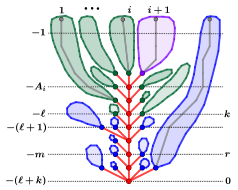
Figure 2: The roots in the green, blue and purple subtrees, represent the set $L_{k}$. The $\sigma$-algebra $\mathcal{F}_{L_{k}}$ is generated by the edges and vertices in red.The $\sigma$-algebra $\mathcal{G}$ is generated by the trees with green roots. At the left hand-side, we have the generation labels as in the planar embedding $\mathbb{Z}_{-}\times\mathbb{N}$. At the right hand-side, we have the generation labels as in the GWVE tree $\mathcal{T}^{(-(\ell+k),\mathfrak{a}_{i}(\ell+k))}$.

By Proposition 2.1, conditionally on $\mathcal{F}_{L}$ the trees $\mathcal{T}^{(x)}$ with roots $x\in R$ and the tree with root in $(-A_{i}+1,\mathfrak{a}_{i+1}(A_{i}-1))$ are independent. In other words, conditionally on $\mathcal{F}_{L}$, the tree $\mathcal{T}^{(-A_{i}+1,\mathfrak{a}_{i+1}(A_{i}-1))}$ and $\mathcal{G}$ are independent. Then, by Proposition III.3.2 in [2]

$$\mathbb{P}\left(\mathcal{T}^{(-A_{i}+1,\mathfrak{a}_{i+1}(A_{i}-1))}={\bf t}\mid\mathcal{G}\vee\mathcal{F}_{L}\right)=\mathbb{P}\left(\mathcal{T}^{(-A_{i}+1,\mathfrak{a}_{i+1}(A_{i}-1))}={\bf t}\mid\mathcal{F}_{L}\right),$$

for every deterministic rooted tree $\bf{t}$. Since $E_{i}\in\mathcal{G}\vee\mathcal{F}_{L}$, we have

$$\mathbb{P}(\mathcal{T}^{(-A_{i}+1,\mathfrak{a}_{i+1}(A_{i}-1))}={\bf t}\mid E_{i}) =\mathbb{P}(\mathbb{P}(\mathcal{T}^{(-A_{i}+1,\mathfrak{a}_{i+1}(A_{i}-1))}={\bf t}\mid\mathcal{G}\vee\mathcal{F}_{L})\mid E_{i})$$

$$=\mathbb{P}(\mathbb{P}(\mathcal{T}^{(-A_{i}+1,\mathfrak{a}_{i+1}(A_{i}-1))}={\bf t}\mid\mathcal{F}_{L})\mid E_{i}).$$ (15)

Now, we use (12) where $m=-\ell$, $x=(-A_{i}+1,\mathfrak{a}_{i+1}(A_{i}-1))$ and $|x|=\ell-A_{i}+1$, to obtain

$$\mathbb{P}(\mathcal{T}^{(-A_{i}+1,\mathfrak{a}_{i+1}(A_{i}-1))}={\bf t}\mid\mathcal{F}_{L})=\mathbb{Q}_{(-A_{i}+1)}\left({\bf t}\right).$$

Hence,

$$\mathbb{P}(\mathcal{T}^{(-A_{i}+1,\mathfrak{a}_{i+1}(A_{i}-1))}={\bf t}\mid E_{i})=\mathbb{P}(\mathbb{Q}_{(-A_{i}+1)}\left({\bf t}\right)\mid E_{i}).$$

Recall that conditional on $E_{i}$, $A_{i}$ only depends on the values of $B_{i}$. Moreover, the vector $(B_{i+1}(1),B_{i+1}(2),\dots,B_{i+1}(A_{i}-1))$ is a functional of the tree $\mathcal{T}^{(-A_{i}+1,\mathfrak{a}_{i+1}(A_{i}-1))}$. Then, given $E_{i}$, the vector $(B_{i+1}(1),B_{i+1}(2),\dots,B_{i+1}(A_{i}-1))$ only depends on the values of $B_{i}$. Let us find its distribution. Let $I(n,j)$ be the smallest index from all the descendants of individual $(-n,\mathfrak{a}_{j}(n))$ at the present generation,

$$I(n,j):=\min\{k\leq j:\mathfrak{a}_{k}(n)=\mathfrak{a}_{j}(n)\},\quad j,n\geq 1.$$

Observe that conditional on $E_{i}$, $I(-A_{i}+1,\mathfrak{a}_{i+1}(A_{i}-1))=i+1$. Then, conditionally on $E_{i}$, for every $1\leq m<A_{i}$,

$$\begin{split}\mathcal{D}_{i+1}(m)&=\{\text{daughters of }(-m,\mathfrak{a}_{i+1}(m))\text{ with descendants in }\{(0,j):j\geq i+1\}\}\\ &=\{\text{daughters of }(-m,\mathfrak{a}_{i+1}(m))\text{ with descendants in }\{(0,j):j\geq 1\}\}.\end{split}$$ (16)

It follows that for every $1\leq m<A_{i}$, the variable $B_{i+1}(m)$ conditioned to $E_{i}$ has the same distribution as $\eta^{(-m)}$ given in (8). Moreover, $B_{i+1}(A_{i})=B_{i}(A_{i})-1$; and for every $A_{i}<m\leq\ell$, we have that $B_{i}(m)=B_{i+1}(m)$. Then, $(B_{i+1}(1),\dots,B_{i+1}(\ell))$ given $E_{i}$, only depends on the values of $B_{i}$.

If $B_{i+1}(m)\neq 0$ for some $1\leq m\leq\ell$, by (10) we have $A_{i+1}\leq\ell$. Recalling equation (7) we conclude that $l_{i+1}=l_{i}\vee A_{i+1}=\ell$ and $B_{i+1}=(B_{i+1}(m),1\leq m\leq\ell)$. Therefore, we have given the distribution of $B_{i+1}$ conditioned on $E_{i}$.

Otherwise, $B_{i+1}(m)=0$ for every $1\leq m\leq\ell$. Similarly, by (7) and (10), we obtain $A_{i+1}>\ell$ and $l_{i+1}>\ell$. Now, by definition of $B_{i+1}$, we need to compute the law of $\{D_{i+1}(m),\ell<m\leq l_{i+1}\}$ and $l_{i+1}$ conditioned on $E_{i}$. In this aim, for a fixed $k\geq 1$, we are going to analyze the tree $\mathcal{T}^{(-(\ell+k),\mathfrak{a}_{i}(\ell+k))}$.

Consider the stopping line $L_{k}$ given by

$$L_{k}=\{\mbox{daughters of }(-n,\mathfrak{a}_{i}(n)):A_{i}\leq n\leq\ell+k\}\setminus\{(-n,\mathfrak{a}_{i}(n)):A_{i}\leq n\leq\ell+k-1\}.$$

As before, $\mathcal{F}_{L_{k}}=\sigma(\Omega_{(-n,\mathfrak{a}_{i}(n))}:A_{i}\leq n\leq\ell+k)$. Observe that $L=L_{1}$ and $E_{i}\in\mathcal{G}\vee\mathcal{F}_{L_{k}}$, where $\mathcal{G}$ is the $\sigma$-algebra generated by the subtrees with roots in $R$ given by (14). See Figure 2. By Proposition 2.1, conditionally on $\mathcal{F}_{L_{k}}$ the subtrees $\mathcal{T}^{(x)}$ with roots $x\in R$ and the subtrees $\mathcal{T}^{(y)}$ with roots $y\in L_{k}\setminus L$ are independent. Therefore, by following the same argument as in (15), for every $y\in L_{k}\setminus L$, we have

$$\mathbb{P}\left(\mathcal{T}^{(y)}={\bf t}\ \Big{|}\ E_{i}\right)=\mathbb{P}\left(\mathbb{P}(\mathcal{T}^{(y)}={\bf t}\mid\mathcal{F}_{L_{k}})\ \Big{|}\ E_{i}\right).$$

Now, if $y\in L_{k}\setminus L$, there exists an $1\leq r<k$ such that $|y|=r$, (recall that $|y|$ denotes its length in $\mathcal{T}^{(-(\ell+k),\mathfrak{a}_{i}(\ell+k))}$). We use (12) to obtain

$$\mathbb{P}(\mathcal{T}^{(y)}={\bf t}\mid\mathcal{F}_{L_{k}})=\mathbb{Q}_{(-(\ell+k)+r)}\left({\bf t}\right).$$

Therefore,

$$\mathbb{P}\left(\mathcal{T}^{(y)}={\bf t}\ \Big{|}\ E_{i}\right)=\mathbb{Q}_{(-(\ell+k)+r)}\left({\bf t}\right).$$ (17)

In words, given $E_{i}$ every subtree with roots in $y\in L_{k}\setminus L$, is still a GWVE tree with environment $\mathcal{S}_{(\ell+k-|y|)}$. Recall that $D_{i+1}(m)=|\mathcal{D}_{i+1}(m)|-1$, where

$$\mathcal{D}_{i+1}(m)=\{\text{daughters of }(-m,\mathfrak{a}_{i+1}(m))\text{ with descendants in }\{(0,j):j\geq i+1\}.$$

Additionally, $\mathfrak{a}_{i}(m)=\mathfrak{a}_{i+1}(m)$, for $m\geq\ell$ and $\ell$ is the coalescent time of individuals $\{(0,j):j\leq i+1\}$. Therefore for every $m\geq\ell+1$, conditionally on $E_{i}$, $\{(0,j):j\leq i+1\}$ are descendant of $(-m,\mathfrak{a}_{i}(m))$ and

$$\mathcal{D}_{i+1}(m)=\{\text{daughters of }(-m,\mathfrak{a}_{i}(m))\text{ with descendants in }\{(0,j):j\geq 1\}\}.$$

Now, we look at the tree $\mathcal{T}^{(-(\ell+k),\mathfrak{a}_{i}(\ell+k))}$. Observe that the daughters of individual $(-m,\mathfrak{a}_{i}(m))$ have length $r=\ell+k-m+1$. Moreover, $(-(m-1),\mathfrak{a}_{i}(m-1))$ is a daughter of $(-m,\mathfrak{a}_{i}(m))$ whose descendants are alive at the present generation. In this way, in the definition of $D_{i+1}(m)$, the minus one can be associated to individual $(-(m-1),\mathfrak{a}_{i}(m-1))$ and, for every $\ell+1\leq m<\ell+k$, the value $D_{i+1}(m)$ can be seen as a functional of the subtrees $\mathcal{T}^{(y)}$ with $y\in L_{k}\setminus L$ such that $|y|=\ell+k-m+1$. By (17), we know that these subtrees, conditioned to $E_{i}$, have law given by $\mathbb{Q}_{(-m+1)}$. Therefore, the distribution of $D_{i+1}(\ell+m)$ conditioned to $E_{i}$ is given by (8), for every $\ell+1\leq m<\ell+k$. Since $k$ was fixed but arbitrary, we have showed that for every $\ell+1\leq m$, the distribution of $D_{i+1}(\ell+m)$ conditioned to $E_{i}$ only depends on $\ell$ and is given by (8).

Recall that the definition of $B_{i+1}$ is the restriction of $D_{i+1}$ to the first $l_{i+1}$ entries, where $l_{i+1}$ is the first $n$ such that $D_{i+1}(n)\neq 0$. Therefore, $l_{i+1}$ conditioned on $E_{i}$ has the same distribution as (11) and we have proved the Markov property with its transitions.

For the law of $A_{1}$ we use equations (9) and (2) to obtain

$$\mathbb{P}(A_{1}>n) =\prod_{i=1}^{n}\mathbb{P}(\eta^{(i)}=0)=\prod_{i=1}^{n}\frac{1-f_{-i+1,0}(0)}{1-f_{-i,0}(0)}f^{\prime}_{-i+1}(f_{-i+1,0}(0))=\frac{f^{\prime}_{-n,0}(0)}{1-f_{-n,0}(0)}.$$

∎

4.2 Proof of Proposition 3.3

We use similar arguments to the previous proof. We explain the differences. By equation (13), we see that $D_{i}(m)=D_{i+1}(m)$ for all $m>A_{i}$ and $D_{i}(A_{i})=D_{i+1}(A_{i})-1$. For $m<A_{i}$, we define

$$G_{i}:=\{D_{j}(n)=d_{j}(n):n\geq 1\,\mbox{ and }\,1\leq j\leq i\}.$$

where $\{d_{j}(n):n\geq 1\,\mbox{ and }\,1\leq j\leq i\}$ are fixed integers. For every $k>A_{i}$, we consider the tree $\mathcal{T}^{(-k,\mathfrak{a}_{i}(k))}$, the stopping line $L_{k}$ given by

$$L_{k}=\{\mbox{daughters of }(-n,\mathfrak{a}_{i}(n)):A_{i}\leq n\leq k\}\setminus\{(-n,\mathfrak{a}_{i}(n)):A_{i}\leq n\leq k-1\},$$

and $R_{k}=L_{k}\setminus\{(-A_{i}+1,\mathfrak{a}_{i+1}(A_{i}-1))\}$. Denote by $\mathcal{G}_{k}$ the $\sigma$-algebra generated by the trees with roots in $R_{k}$. As in the proof of Theorem 3.2, $\mathcal{F}_{L_{k}}=\sigma(\Omega_{(-n,\mathfrak{a}_{i}(n))}:A_{i}\leq n\leq k)$. By Proposition 2.1, conditionally on $\mathcal{F}_{L_{k}}$, the tree $\mathcal{T}^{(-A_{i}+1,\mathfrak{a}_{i+1}(A_{i}-1))}$ and $\mathcal{G}_{k}$ are independent. Then,

$$\mathbb{P}\left(\mathcal{T}^{(-A_{i}+1,\mathfrak{a}_{i+1}(A_{i}-1))}={\bf t}\mid\mathcal{G}_{k}\vee\mathcal{F}_{L_{k}}\right)=\mathbb{P}\left(\mathcal{T}^{(-A_{i}+1,\mathfrak{a}_{i+1}(A_{i}-1))}={\bf t}\mid\mathcal{F}_{L_{k}}\right),$$

for every deterministic rooted tree $\bf{t}$. We observe that $\mathcal{G}_{k}\subset\mathcal{G}_{k+1}$ and $\mathcal{F}_{L_{k}}\subset\mathcal{F}_{L_{k+1}}$ for all $k$. Let $\mathcal{G}:=\lim_{k}\mathcal{G}_{k}$ and $\mathcal{F}:=\lim_{k}\mathcal{F}_{L_{k}}$. Note that $G_{i}$ is $(\mathcal{G}\vee\mathcal{F})$-measurable. Therefore, by the Monotone Convergence Theorem and the previous equation,

$$\mathbb{P}(\mathcal{T}^{(-A_{i}+1,\mathfrak{a}_{i+1}(A_{i}-1))}={\bf t}\mid G_{i}) =\mathbb{P}(\mathbb{P}(\mathcal{T}^{(-A_{i}+1,\mathfrak{a}_{i+1}(A_{i}-1))}={\bf t}\mid\mathcal{G}\vee\mathcal{F})\mid G_{i})$$

$$=\mathbb{P}(\lim_{k}\mathbb{P}(\mathcal{T}^{(-A_{i}+1,\mathfrak{a}_{i+1}(A_{i}-1))}={\bf t}\mid\mathcal{G}_{k}\vee\mathcal{F}_{L_{k}})\mid G_{i})$$

$$=\mathbb{P}(\lim_{k}\mathbb{P}(\mathcal{T}^{(-A_{i}+1,\mathfrak{a}_{i+1}(A_{i}-1))}={\bf t}\mid\mathcal{F}_{L_{k}})\mid G_{i}).$$

Now, we use (12), to obtain

$$\mathbb{P}(\mathcal{T}^{(-A_{i}+1,\mathfrak{a}_{i+1}(A_{i}-1))}={\bf t}\mid\mathcal{F}_{L_{k}})=\mathbb{Q}_{(-A_{i}+1)}\left({\bf t}\right),\qquad\mbox{ for all }\quad k>A_{i}.$$

Hence,

$$\mathbb{P}(\mathcal{T}^{(-A_{i}+1,\mathfrak{a}_{i+1}(A_{i}-1))}={\bf t}\mid G_{i})=\mathbb{P}(\mathbb{Q}_{(-A_{i}+1)}\left({\bf t}\right)\mid G_{i}).$$

Observe that conditional on $G_{i}$, $A_{i}$ only depends on the values of $D_{i}$. Moreover, the vector $(D_{i+1}(1),D_{i+1}(2),\dots,D_{i+1}(A_{i}-1))$ is a functional of the tree $\mathcal{T}^{(-A_{i}+1,\mathfrak{a}_{i+1}(A_{i}-1))}$. Then, $(D_{i+1}(1),B_{i+1}(2),\dots,D_{i+1}(A_{i}-1))$ given $G_{i}$, only depends on the values of $D_{i}$. This implies the Markov property. By continuing with the same arguments as in the proof of Theorem 3.2, we get (16) and from there we obtain its distribution. ∎

4.3 Proof of Proposition 3.4

Observe that for every $n\geq 1$, the variable $\eta^{(-n)}\overset{\mathcal{L}}{=}\eta_{n}$ with environment $\mathcal{E}_{n}=(e_{-n+1},e_{-n+2},\dots,e_{0})$ as in Example 2.2. In particular, $\eta^{(-n)}$ has geometric distribution (modeling the number of failures until the first success) with success probability $\lambda_{1}:=p_{0}$ and for $n\geq 2$,

$$\lambda_{n}:=\left(1+\underset{k=-n+2}{\overset{0}{\sum}}s_{k}\right)\left(1+\underset{k=-n+1}{\overset{0}{\sum}}s_{k}\right)^{-1}.$$ (18)

where $s_{0}=\tfrac{1-p_{0}}{p_{0}}$ and $s_{k}=\tfrac{(1-p_{k})}{p_{k}}\tfrac{r_{k+1}\cdots r_{0}}{p_{k+1}\cdots p_{0}}\,$ for $k<0$. By induction on $i\geq 1$, we are going to prove the following statement:

(${H_{i}}$)

The random variables $(D_{i}(n),n\geq 1)$ are independent, geometrically distributed with success probability $\lambda_{n}$ given in (18). In addition, they are independent of $(A_{0},\dots,A_{i-1})$.

The claim holds once we prove that $(H_{i})$ is true for every $i\geq 1$. Indeed, suppose that $(H_{i})$ is true for every $i\geq 1$. Then, by equation (6), we can see that $A_{i}$ is independent of $(A_{0},\dots,A_{i-1})$ and it is distributed as $A_{1}$. In particular,

$$\mathbb{P}(A_{i}>n)=\prod_{\ell=1}^{n}\mathbb{P}(\eta^{(\ell)}=0)=\left(1+\underset{k=-n+1}{\overset{0}{\sum}}s_{k}\right)^{-1},\qquad n\geq 1.$$

Observe that $(H_{1})$ holds by Corollary 3.3. Now, we assume $(H_{i})$ and we will prove that $(H_{i+1})$ is also true by conditioning on the value of $A_{i}$. Suppose that $A_{i}=h$. We now apply the transition probabilities from Corollary 3.3. Note that $D_{i}(n)=D_{i+1}(n)$ for all $n>h$. Then, by hypothesis $(H_{i})$, the variables $(D_{i+1}(n),n>h)$ are independent, geometrically distributed with parameters $\lambda_{n}$ and also independent of $(A_{0},\dots,A_{i-1})$. For $n=h$, by hypothesis, $D_{i+1}(h)=D_{i}(h)-1$ is independent of $(D_{i}(n),n>h)$ and independent of $(A_{0},\dots,A_{i-1})$. In addition, by (6), $D_{i}(h)$ is a geometric variable with parameter $\lambda_{h}$ conditioned to be strictly positive. Then,

$$\mathbb{P}(D_{i+1}(h)=k)=\frac{\mathbb{P}(\eta^{(h)}=k+1)}{\mathbb{P}(\eta^{(h)}>0)}=\lambda_{h}(1-\lambda_{h})^{k},\qquad k\geq 0,$$

is a geometric random variable with parameter $\lambda_{h}$. Finally, the variables $(D_{i+1}(n),n<h)$ are new independent geometric random variables with parameters $\lambda_{n}$ (therefore, they are independent of $(D_{i+1}(n),n\geq h)$ and $(A_{0},\dots,A_{i-1})$). In other words, conditionally on $\{A_{i}=h\}$, the variables $(D_{i+1}(n),n\geq 1)$ are independent with geometric distributions of parameters $\lambda_{n}$ and independent of $(A_{0},\dots,A_{i-1})$. It remains to integrate over $h$ to obtain the result $(H_{i+1})$. ∎

References

[1]
Chauvin, B.: Sur la propriété de branchement. Ann. Inst. Henri Poincaré B 22 (1986), 233–236.
[2] Çınlar, E.: Probability and stochastics. Graduate Texts in Mathematics, 261, Springer, New York, (2011), xiv+557 pp.
[3] Kersting, G. and Vatutin, V.: Discrete time branching processes in random environment. Wiley Online Library, (2017), 306 pp.
[4] Kyprianou, A. E. (2000). Martingale convergence and the stopped branching random walk. Probability theory and related fields, 116(3), 405-419.
[5] Jagers, P. General branching processes as Markov fields. Stochastic Processes and their Applications, 32.2 (1989): 183-212.
[6] Lambert, A. and Popovic, L.: The coalescent point process of branching trees. Annals of Applied Probability23, (2013), no. 1, 99–144.
[7] Popovic, L and Rivas, M.: The coalescent point process of multi-type branching trees. Stochastic Processes and their Applications124, (2014), no. 12, 4120–4148.
[8] Rannala, B.: On the genealogy of a rare allele. Theoretical Population Biology52, (1997), no. 3, 216–223.
Acknowledgments
We are grateful to Amaury Lambert and Lea Popovic for the discuss and comments. S. P. was supported by UNAM-DGAPA-PAPIIT grant no. IA103220.