An ALMA search for high albedo objects among the mid-sized Jupiter Trojan population

Abstract

We use ALMA measurements of 870 $\mu$m thermal emission from a sample of mid-sized (15-40 km diameter) Jupiter Trojan asteroids to search for high albedo objects in this population. We calculate the diameters and albedos of each object using a thermal model which also incorporates contemporaneous Zwicky Transient Facility photometry to accurately measure the absolute magnitude at the time of the ALMA observation. We find that while many albedos are lower than reported from WISE, several small Trojans have high albedos independently measured both from ALMA and from WISE. The number of these high albedo objects is approximately consistent with expectations of the number of objects that recently have undergone large-scale impacts, suggesting that the interiors of freshly-crated Jupiter Trojans could contain high albedo materials such as ices.

1 Introduction

The Jupiter Trojan asteroids, at the intersection of the inner and outer solar system, hold some of the keys to understanding the formation and early dynamical evolution of the entire solar system. In the modern incarnation of the Nice model of dynamical instability, the Jupiter Trojans formed beyond the region of the giant planets, at the same location as the objects currently in the Kuiper belt (Morbidelli et al., 2005; Morbidelli, 2010). Previous hypotheses had instead suggested that the Jupiter Trojans formed in the main asteroid belt or closer to the Jupiter system, and that they share no relationship with objects in the Kuiper belt (Marzari & Scholl, 2002). Connecting the compositions of the Jupiter Trojans and the Kuiper belt objects (or finding that they are not connected) is critical to answering fundamental questions about the nature of the early dynamical evolution of the solar system.

Unfortunately, we have essentially zero knowledge of the interior compositions of Jupiter Trojans. After 4 billion years of space weathering, the surfaces of the Jupiter Trojans are now covered with a thick irradiated mantle that mostly defies spectroscopic identification (Fornasier et al., 2007; Emery et al., 2011; Brown, 2016). One solution to the lack of access to the interiors of Jupiter Trojans is to search for objects that have suffered recent massive collisions and have some of their interior materials freshly exposed.

Freshly exposed interior material from the main asteroid belt and from the Kuiper belt have very different compositions. The Haumea collision family – the one known collisional family in the Kuiper belt – is composed of objects with nearly pure water ice surfaces (Brown et al., 2007), even billions of years after the family-forming impact (Ragozzine & Brown, 2007). These objects are unique in the observed Kuiper belt. In contrast, even the youngest known collisional family in the main belt, the Karin family, at only $\sim$6 Myr old, has family members whose surfaces are indistinguishable from the background population (Harris et al., 2009). We expect this general principle to hold: fresh collisional fragments of objects from the inner and outer solar system should be distinguishable by their distinct compositions.

If the interiors of Jupiter Trojans are composed of outer solar system ices, we should expect that fragments left over after a catastrophic collision would have high albedos, yet no evidence exists for albedo differences between members of the Trojan asteroids’ best-known collisional family –- the Eurybates family (De Luise et al., 2010) –- and the rest of the Trojan population. Either the interiors of these objects do not contain high-albedo material, or irradiation, devolatilization, and space weathering have hidden the albedo signature of the fresh materials over time. The Eurybates family is presumably ancient, but impacts younger than the $\sim$100 Myr timescale of space weathering (Thompson et al., 1987; Brunetto et al., 2006) could still have regions of elevated albedo.

Collisonal models suggest that collisional fragments from $\sim$100 Myr old catastrophic impacts are likely common among the smallest known Jupiter Trojans ($\sim$1 km) (de Elía & Brunini, 2007), but these objects are prohibitively faint for detailed study. While larger (and thus brighter) collisional fragments are rare, a small number of them must exist in the Trojan population. Based on collisional models, about 5% of Trojans in the 20–30 km size range will have had catastrophic impacts in the past 100 Myr (de Elía & Brunini, 2007), with many more having significant sub-catastrophic cratering events. It is in this size range where, if the interiors of Jupiter Trojans contain high albedo materials such as ices, we might expect to find a small number of objects with elevated albedos. If such larger recent collisional fragments can be found, their larger size and brightness would make them attractive targets for detailed spectroscopy to understand the interior compositions of Jupiter Trojans.

At first glance, measurements from the WISE spacecraft appear to support the expectation that a small number of 20–30 km Jupiter Trojans indeed have elevated albedos, but the reliability of the derived albedos is uncertain. WISE detected 476 Jupiter Trojan asteroids at some combination of wavelengths including 3.3, 4.6, 12.1, and 22.2 $\mu$m (Grav et al., 2012). The two longest wavelengths sample the short-wavelength tail of the blackbody emission of these objects, allowing radiometric determination of their diameters and albedos. Unlike in the main asteroid belt or even in the Kuiper belt, the albedos of the Trojans appear strikingly uniform (at least among the well-sampled large objects), with a median albedo of 0.069. There is a hint in the WISE data that albedos may rise below a diameter of 30 km, but much of this apparent rise could be driven by the larger uncertainties in the thermal fluxes of these smaller objects, the positive bias in albedo, and bias from the optically-selected sample. In addition, measuring the albedo using only the exponentially changing short-wavelength end of the blackbody emission is highly sensitive to model assumptions and parameters. With these caveats, a small number of objects appear to have sufficiently high albedos and sufficiently small uncertainties that their albedos are statistically inconsistent with the median value (Figure 1). Visible and infrared spectroscopy of a subset of these from the Very Large Telescope shows nothing unusual, but the limits on detection of water ice, for example, which has only relatively weak absorption features shortward of 2.5 $\mu$m, are not strong (Marsset et al., 2014).

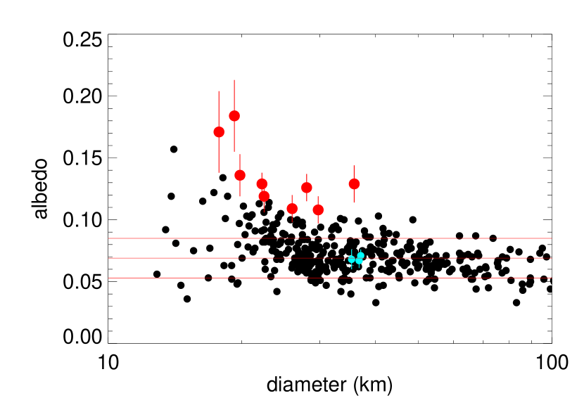
Figure 1: Derived albedos and diameters based on WISE observations (Grav et al., 2012). The black points show all Trojans for which the WISE-derived albedo uncertainties are 0.02 or lower. The median and 1$\sigma$ variation of albedo of these Trojans are shown as red horizontal lines. The nine objects shown in red all have WISE-derived albedos and uncertainties that appear to be 3$\sigma$ or more above the median Trojan albedo. Also shown, in cyan, are three objects measured by WISE to have typical albedos; these targets are used as emissivity calibrators for the survey.

Table 1: Observational Details for each object. The observation time and length is given, as well as the heliocentric and geocentric distances of the object alongside the flux density for each observation.

Object	Midpoint	Total time	Geocentric	Heliocentric	Phase Angle	Flux Density
			distance (AU)	distance (AU)	(degrees)	(mJy)
05123 (1989 BL)	2019 Oct 06 23:02	5 min	5.08	5.66	8.7	1.39 $\pm$ 0.07
08125 (Tyndareus)	2019 Oct 06 02:52	5 min	4.01	4.96	4.0	1.4 $\pm$ 1.0
	2019 Oct 07 02:45	5 min	4.01	4.96	4.1	1.18 $\pm$ 0.07
11488 (1988 RM11)	2019 Oct 08 20:28	18 min	6.21	5.33	4.6	0.24 $\pm$ 0.06
	2019 Oct 09 15:48	18 min	6.22	5.33	4.5	0.18 $\pm$ 0.04
13331 (1998 SU52)	2019 Oct 06 23:32	24 min	4.62	5.21	9.4	0.22 $\pm$ 0.03
13372 (1998 VU6)	2019 Oct 06 02:28	18 min	4.36	5.12	7.9	0.51 $\pm$ 0.05
13694 (1997 WW7)	2019 Oct 06 03:11	12 min	4.04	5.01	2.7	0.86 $\pm$ 0.06
18054 (1999 SW7)	2019 Oct 08 20:03	5 min	5.98	5.15	5.7	0.50 $\pm$ 0.09
	2019 Oct 10 18:36	5 min	5.99	5.15	5.5	0.68 $\pm$ 0.09
18137 (2000 OU30)	2019 Oct 06 15:18	5 min	6.15	5.15	0.7	0.43 $\pm$ 0.09
	2019 Oct 09 14:53	5 min	6.15	5.15	0.9	0.47 $\pm$ 0.07
18263 (Anchialos)	2019 Oct 06 04:03	18 min	4.24	5.20	3.4	0.34 $\pm$ 0.05
	2019 Oct 07 03:19	18 min	4.25	5.20	3.6	0.33 $\pm$ 0.04
24452 (2000 QU167)	2019 Oct 10 16:01	18 min	6.34	5.43	4.1	0.15 $\pm$ 0.05
	2019 Oct 10 17:57	18 min	6.34	5.43	4.1	0.21 $\pm$ 0.05
32501 (2000 YV135)	2019 Oct 10 15:36	5 min	5.79	4.87	4.1	0.5 $\pm$ 0.2
	2019 Oct 10 17:02	5 min	5.80	4.87	4.0	0.6 $\pm$ 0.1
42168 (2001 CT13)	2019 Oct 06 03:34	12 min	4.05	4.98	4.6	0.31 $\pm$ 0.05

These high-albedo objects could be the collisional fragments of recent impacts. Indeed, models suggest that this is approximately the expected number of objects that should have had catastrophic impacts in the past 100 Myr. Unfortunately, an alternative possibility is that the putative high-albedo objects are normal low albedo Trojans and that observational and modeling uncertainties have been underestimated. Determining sizes and albedos of objects is particularly hard when all thermal observations are on the steep Wein section of the blackbody curve where small changes in modeling assumptions can lead to exponential changes in flux density. Calibration of the WISE flux densities to better than 10% is hampered by uncertainties in the color correction required for low temperatures of these distant targets (Wright et al., 2010).

In order to independently estimate the albedos of these potentially high-albedo objects, we obtained 870 $\mu$m radiometry of 9 of these objects using the Atacama Large Millimeter Array (ALMA). In addition, we observe 3 Trojan asteroids with well-measured albedos consistent with the albedos measured for the larger members of the population and use these measurements to calibrate the millimeter emissivity. Observing these targets from ALMA has two main advantages: first, we can control the signal-to-noise (S/N) of the detections by varying the exposure time, rather than having to rely on the uniform WISE survey, and thus are not as affected by a falling S/N at smaller sizes. Second, at these wavelengths, which cover the Rayleigh-Jeans portion of the blackbody, the flux density is only linearly, rather than exponentially, sensitive to surface temperature, making the observations significantly less sensitive to modeling assumptions. We use the observations as well as contemporaneous observations of the visible flux from these objects using the Zwicky Transient Facility (ZTF) archive to investigate the albedos of these potentially high albedo objects.

2 OBSERVATIONS AND DATA REDUCTION

The observations of the Trojan asteroids were taken with the main array of ALMA, which is composed of up to 50 12-meter diameter antennas spread across the Altiplano in the high northern Chilean Andes. ALMA can operate in 7 frequency windows, from $\sim$90 to $\sim$950 GHz. The observations presented here were taken in Band 7, near 340 GHz, in the “continuum” (or “TDM”) mode, with standard frequency tuning. This set up results in four spectral windows with frequencies of 335.5–337.5 GHz, 337.4–339.4 GHz, 347.5–349.5 GHz, and 349.5–351.5 GHz. In the final steps of the data reduction, we averaged over the entire frequency range, and use 343.5 GHz (872.8 $\mu$m) as the observation frequency in our thermal modelling.

We observed with ALMA on dates from October 6 to 10 of 2019 (Table 1). For these observations, there were between 41 and 46 antennas, mostly in the C43-4 configuration. In the earlier observations (October 6-7), some antennas were on pads isolated from the rest of the array, and, to be conservative, we exclude those antennas from later analysis, thus between 38 and 46 antennas are used in the final analysis. The C43-4 configuration has a maximum antenna spacing of $\sim$784 m, giving a maximum resolution on the sky of $\sim$300 mas at our observing frequency, much larger than the $\sim$ 20 mas apparent diameter of any of the Trojan asteroids.

Observations lasted from 16 to 40 minutes in duration, including all calibration overheads, which resulted in 5 to 24 minutes on the asteroid. One of six “grid calibrators” was used as the absolute flux density scale calibrator for the observations, depending on where in the sky the targets were at the time. These grid calibrators are regularly monitored against the main flux density scale calibrators for ALMA. The absolute flux density scale calibration which results is believed to be good to 5% in Band 7 for ALMA, but can in some cases be worse (Francis et al., 2020). Nearby point-like calibrators were used to calibrate the phase of the atmosphere and antennas as a function of time.

Initial calibration of the data was provided by the ALMA observatory, completed in the CASA reduction package via the ALMA pipeline (Muders et al., 2014). We exported the provided visibilities from CASA and continued the data reduction in the AIPS reduction package. We flagged outlier antennas, then made a decorrelation correction to each observation. Such a correction is necessary because even after normal calibration, phase errors remain in the data, and an estimate of their effect on the visibilities must be made in order to derive meaningful flux densities (Thompson et al., 2017). If the asteroids had enough flux density to self-calibrate, we could use that to correct these phase errors, but they do not. Fortunately, however, ALMA included “check sources” in each of these observations. These are nearby point sources that do have enough flux density to be self-calibrated, and are observed and calibrated in the same way as the target source. So estimating flux density before self-calibration, then after, for these check sources gives a correction factor which we applied to the data. We then did a fit of the asteroid visibilities to a point source, along with making an image. The fit to the visibilities provides a more reliable flux density, since it is not subject to imaging deconvolution errors. But in all cases, the fit to the visibilities and the fit to a Gaussian in the image agreed to within one-sigma. For the asteroids which had two separate observations, we fitted each one separately, then combined the data and fit that as well. The resultant fitted flux densities are shown in Table 2.

Table 2: Rotation periods, combined flux densities, and absolute magnitudes for each object. Where no period was able to be determined using the ZTF data, the period column is left blank. If multiple periods are possible all are listed as well as the phased absolute magnitude for each potential period.

	Period	Flux Density	Absolute
Object	(h)	(mJy)	Magnitude
05123 (1989 BL)	$9.897\pm 0.008$	$1.39\pm 0.07$	$10.1\pm 0.1$
08125 (Tyndareus)	$51.2\pm 0.2$	$1.26\pm 0.06$	$11.02\pm 0.09$
11488 (1988 RM11)	——	$0.20\pm 0.03$	$11.44\pm 0.04$
13331 (1998 SU52)	$373.5\pm 13.8$	$0.22\pm 0.03$	$11.59\pm 0.06$
13372 (1998 VU6)	——	$0.51\pm 0.05$	$11.34\pm 0.05$
13694 (1997 WW7)	$19.95\pm 0.02$	$0.86\pm 0.06$	$11.12\pm 0.06$
	$34.14\pm 0.06$	"	$11.09\pm 0.06$
18054 (1999 SW7)	——	$0.59\pm 0.06$	$10.75\pm 0.07$
18137 (2000 OU30)	$12.102\pm 0.007$	$0.45\pm 0.06$	$11.26\pm 0.07$
	$16.20\pm 0.01$	"	$11.27\pm 0.09$
	$24.47\pm 0.05$	"	$11.17\pm 0.07$
18263 (Anchialos)	$10.330\pm 0.006$	$0.33\pm 0.03$	$11.58\pm 0.07$
24452 (2000 QU167)	——	$0.18\pm 0.03$	$11.94\pm 0.07$
32501 (2000 YV135)	——	$0.59\pm 0.09$	$11.38\pm 0.07$
42168 (2001 CT13)	$4.499\pm 0.002$	$0.31\pm 0.05$	$11.53\pm 0.09$
	$4.966\pm 0.002$	"	$11.43\pm 0.07$
	$5.540\pm 0.002$	"	$11.38\pm 0.07$
	$6.265\pm 0.003$	"	$11.41\pm 0.07$
	$7.206\pm 0.004$	"	$11.55\pm 0.07$
	$8.482\pm 0.005$	"	$11.66\pm 0.07$
	$10.308\pm 0.008$	"	$11.68\pm 0.07$
	$13.14\pm 0.01$	"	$11.55\pm 0.07$

3 Zwicky Transient Facility photometry

Radiometric measurement of diameter and albedo requires not just thermal emission, but an accurate measurement of the visible magnitude at the time of the thermal observation. In practice determining such a magnitude requires determining both the rotational amplitude of the object and the phase at the time of the ALMA observation. These parameters are generally unknown for our targets. Fortunately, ZTF was engaged in a large scale photometric sky survey at the time of our ALMA observations. All targets were observed a minimum of 27 times during the 2019 opposition season with one- to several-day spacings. Schemel & Brown (2020) analyzed the photometric data from $\sim$1000 Trojans asteroids and developed a powerful method to extract absolute magnitudes, colors, phase curves, and rotational amplitudes from these sparsely sampled data. For most objects, however, they did not attempt to determine the rotation period, which we need to correctly phase the data. We further analyze the ZTF data with the goal to directly determine the absolute magnitude at the time of the observation.

For each of the ALMA targets, we take the ZTF photometric data from Schemel & Brown (2020), convert it to a V-band absolute magnitude using the derived color and phase curve and the appropriate conversion from Jester et al. (2005) for solar colors, and subtract the average magnitude, yielding observations that should only be affected by the light curve of the asteroid. The time series of these residual magnitudes was then examined for a periodic behaviour. For each object, the Astropy implementation of a Lomb-Scargle periodogram was used to construct a periodogram showing the power at different frequencies. In many cases, we find a single strong peak with aliases at frequencies corresponding to frequencies separated by $\sim$1 day^-1, as expected from these nightly-sampled data. To calibrate the significance of the periodogram peaks, the data were shuffled by randomly assigning each observed photometric point to an observed observation time. A periodgram of these shuffled data will show the effects of the noise and the observing cadence on the periodogram. We perform 100 iterations of this shuffling and retain the maximum periodogram power over the entire frequency range over all iterations as our limit of significance.

As an additional test of the significance of the periodic fits, we calculate the Akaike Information Criterion (specifically the version corrected for smaller sample sizes, knowns as AIC_C). The AIC_C is defined as:

$${\rm AIC}_{C}\equiv 2k-2\ln\mathcal{L_{\rm max}}+{{2k^{2}+2k}\over{n-k-1}}$$

where $\mathcal{L}_{\rm max}$ is the value of the maximum likelihood, $k$ is the number of free parameters, and $n$ is the number of data points. The model with the lower value of AIC_C is prefered by a factor of $\exp[(\Delta{\rm AIC}_{C})/2],$ where $\Delta$AIC_C is the difference in AIC_C between the two models (Burnham & Darling, 2004), which, in our case, is the difference between a model of constant magnitude and a simple sinusoidal maximum likelihood fit at the selected period. In all cases where we list a potential period fit, $\Delta$AIC${}_{C}>$16, implying that the periodic fit is preferred by more than a factor of 3000. In the majority of cases $\Delta$AIC${}_{C}>100$.

Fig 2 shows an example of this procedure from object 18263. The other Trojan asteroids for which potential periods were found are shown in the Appendix.

For each possible period over the significance threshold we performed multiple steps to determine the viability of the potential period. We first phased all data to each potential period. As expected from the periodograms, all data were consistent with each significant period, with the quality of the fit decaying as the periodogram power dropped. Next, we attempted to confirm rotational periods from published values. Objects 5123 and 13331 were observed in the Kepler K2 mission and analyzed in Szabó et al. (2017) and Ryan et al. (2017). Based on these results, all but one potential period could be ruled out for these two objects. In addition, previous data for 13694, 18263, and 18137 as presented in French et al. (2012), French et al. (2015), and Stephens et al. (2015) respectively, were used to check the viability of periods found using ZTF data. Previously observed data for each of these objects was obtained from the Asteroid Lightcurve Photometry Database (Stephens et al., 2010; Warner et al., 2011) and these magnitudes were phased to each potential period indicated by the periodogram. In cases where the additional data did not produce a consistent lightcurve when phased to a given period, that period could be discarded, thus reducing the number of potential periods for these three objects. For object 32501, many periods were above the significance threshold, and its relatively flat lightcurve prevented any assessment of whether these periods indicated actual periodic variation in the lightcurve. In addition, for object 8125, all but one potential period was discarded as the phased lightcurve was not consistent with periodic behavior. The period for each object, or, in some cases, the multiple possible periods, are shown in Table 2. Note that we assume that all light curves are mostly due to shape and thus have two full cycle per rotation. The listed periods are thus twice that of the best single-cycle periods found in the periodograms. The uncertainties on the periods listed in Table 2 are better than the literature values for 5123 (Ryan et al., 2017), 18263 (French et al., 2015), and that for the 16.2 day period for 18137 (Stephens et al., 2015).

With periods or groups of possible periods for all objects now determined, we determined the shape of each light curve by using each possible period to phase all ZTF data taken within 6 months of the the ALMA observation (the full ZTF data set was not used owing to slow viewing-angle changes over time that can change the shape – but not period – of the light curve). We use a fourth-order Fourier series to better fit the full asymmetric light curve from each data set. To understand the full range of uncertainties from such a fit we create a likelihood model with the four Fourier parameters as our model parameters and use a Markov-Chain Monte Carlo (MCMC) procedure – as implemented in the emcee package (Foreman-Mackey et al., 2013) – to sample the four-dimensional phase space of Fourier coefficients. All MCMC chains were run to a length of 5600 samples, more than 50 times the autocorrelation length, and the first 800 samples of each chain were discarded as burn-in. From each Markov Chain sample we create a light curve and determine the absolute magnitude at the time of the observation. The best-fit absolute magnitude is then taken to be the median of the value predicted for that time given the sample coefficients. The uncertainties appear essentially Gaussian thus we take the $1\sigma$ variation in magnitude to be the 16th and 84th percentile values of the absolute magnitude.

Figure 2 illustrates this process, showing the initial periodogram obtained for object 18263. All but one potential period was discarded by cross-checking the periods with data in the literature, so only one frequency is indicated on the periodogram. Beneath, we plot the phased ZTF data as well as a random selection of MCMC light curve samples to illustrate the uncertainties.

Some objects have little constraint on the rotation period and have no value listed in Table 2, owing either to a small light curve or to other unknown factors, so we are able to obtain neither a period nor a phase for the ALMA observation. For these objects we simply take the mean absolute magnitude for the 2019 season and use the full amplitude of the light curve from Schemel & Brown (2020) as the uncertainty.

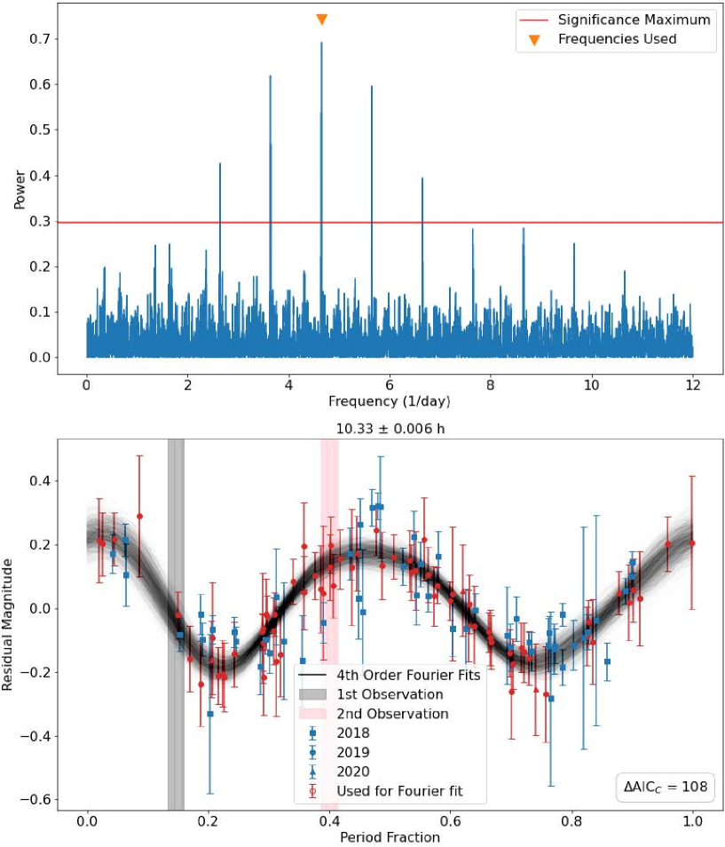
Figure 2: Periodogram and phased ZTF lightcurve for object 18263. While multiple periods are above the significance threshold, only one (the highest peak) is consistent with previous data. The ZTF data phased to that period is plotted below it. The shape of each data point indicates the year in which that data point was taken. The red points indicate which data were used to find the best fit fourth order Fourier series using an MCMC.  The value of $\Delta$AOI_C calculated for the periodic fit compared to a constant light curve is shown in the bottom right (see text for details). Random samples of the results of this fitting process are plotted as dark lines over the data. The grey and red shaded regions indicate where in the curve the ALMA observations occurred.

4 Thermal Model

In order to obtain values of physical properties – including albedo – based on the thermal emission observed, a thermal model similar to that given in Harris (1998) is used. This model predicts thermal flux at any wavelength based on albedo, diameter, and the object’s heliocentric and geocentric distances. In addition, the model used here includes a variable beaming parameter, a catch-all factor accounting for surface roughness and other irregularities in the object’s emission, rather than a single value to account for this effect for all objects. The model also allows the millimeter emmisivity of Trojans as a free parameter to be calibrated later.

The model assumes a spherical object and calculates the instantaneous equilibrium temperature at each point on the day hemisphere. For an object receiving a solar flux $S$ with bond albedo $A$, bolometric emissivity $\epsilon$, and beaming parameter $\mu$, the temperature at each angle from the subsolar point $\omega$ is, with $\sigma$ as the Stefan-Boltzmann constant:

$$T=\left(\frac{[1-A]S\cos{\omega}}{\mu\epsilon\sigma}\right)^{1/4}.$$ (1)

The Bond albedo is related to the geometric albedo $p_{v}$ as $A=qp_{V}$, where $q$ is the phase integral. The correct phase integral to be used here is not obvious, but for the generally low albedos expected here changes in the value of $q$ make only minor changes in derived parameters. We thus use the standard formulation derived by Bowell et al. (1989) of $q=0.24+0.684G$, where $G$ is the phase parameter. Schemel & Brown (2020) find a median value of $G=0.24$ for Jupiter Trojans, giving a value of $q=0.45$.

With the temperatures at each angle from the subsolar point found, the emission at the wavelength of the ALMA observations can be calculated and summed over the surface of the object, accounting for its diameter, emissivity, and its distance from the Sun and Earth. In addition, the absolute magnitude $H_{V}$, albedo, and diameter $D$ of an object are related as:

$$H_{V}=-5\log{{}_{10}(D\sqrt{p_{V}}/1330)}$$ (2)

The absolute magnitudes used in the WISE analysis are consistently lower than those found from the ZTF analysis performed in Schemel & Brown (2020), with an average difference of 0.32 magnitudes for the twelve objects in our sample. Applying this offset to the full WISE dataset gives a new mean Jupiter Trojan albedo of 0.051. We take this as the canonical value and now use the three calibrator targets (18054, 18137, and 32501) to determine an average value for millimeter emissivity. To do so we create a likelihood model relating our model parameters to the observations by using the thermal model to produce a flux density and an absolute magnitude given diameter, albedo, and beaming parameter as input parameters. We use this likelihood model in an MCMC model to sample this phase space, again employing the emcee package from Foreman-Mackey et al. (2013). We have no observational constraints on beaming parameter in our data, so we use the full distribution of values found in Grav et al. (2012) as our prior. Priors in the other parameters were uniform and positive (and less than one, for albedo). All MCMC chains were run to a length of 5000 samples, more than 100 times the autocorrelation length, and the first 500 samples of each chain were discarded as burn-in. The marginalized posterior distributions are nearly gaussian, and with the expected anti-correlation between diameter and albedo. We manually adjust the emissivity of the calibrator objects to force the three objects to have an average albedo of 0.051. Our derived emissivity is 0.753.

Using this derived emissivity for our entire sample, we now run the MCMC model on all nine putatively high-albedo targets, again running each chain more than 100 times the autocorrelation length. We report median values of the derived parameters with uncertainties giving the 14% and 86% percentiles of the distribution in Table 3.

Table 3: Diameter and albedos obtained using the MCMC procedure to determine best fit thermal models. Errors were obtained using the distribution of each parameter from the MCMC procedure. If the distribution was relatively symmetric, only a single uncertainty is given; otherwise, upper and lower errors are both stated. If the object has multiple possible rotational periods, the average albedo with the maximum range of uncertainty is also given on the first entry for each object.

object	period (h)	diameter (km)	albedo	adopted albedo
05123	$9.897\pm 0.008$	$50.3_{-1.1}^{+1.2}$	$0.063_{-0.005}^{+0.006}$	$0.063_{-0.005}^{+0.006}$
08125	$51.2\pm 0.2$	$36.4\pm 0.8$	$0.052\pm 0.004$	$0.052\pm 0.004$
11488	——	$22.7\pm 1.4$	$0.09\pm 0.01$	$0.091_{-0.010}^{+0.012}$
13331	$373.5\pm 13.8$	$17.7\pm 0.9$	$0.132_{-0.013}^{+0.015}$	$0.132_{-0.013}^{+0.015}$
13372	——	$25.4_{\pm}0.9$	$0.080\pm 0.006$	$0.080\pm 0.006$
13694	$19.95\pm 0.02$	$30.4_{-0.8}^{+0.9}$	$0.068\pm 0.005$	$0.069_{-0.005}^{+0.006}$
	$34.14\pm 0.06$	$30.4\pm 0.9$	$0.070\pm 0.005$
18054	——	$37.4\pm 1.5$	$0.063_{-0.005}^{+0.006}$	$0.063_{-0.005}^{+0.006}$
18137	$12.102\pm 0.007$	$33.6\pm 1.6$	$0.049\pm 0.005$	$0.050_{-0.007}^{+0.009}$
	$16.20\pm 0.01$	$33.7_{-1.6}^{+1.5}$	$0.049_{-0.005}^{+0.006}$
	$24.47\pm 0.05$	$33.7_{-1.6}^{+1.5}$	$0.053_{-0.005}^{+0.006}$
18263	$10.330\pm 0.006$	$20.1\pm 0.7$	$0.102_{-0.008}^{+0.009}$	$0.102_{-0.008}^{+0.009}$
24452	——	$21.9_{-1.6}^{+1.5}$	$0.06\pm 0.01$	$0.06\pm 0.01$
32501	——	$35.5_{-2.1}^{+2.0}$	$0.039_{-0.004}^{+0.005}$	$0.039_{-0.004}^{+0.005}$
42168	$4.499\pm 0.002$	$18.1\pm 1.1$	$0.13\pm 0.02$	$0.13_{-0.03}^{+0.04}$
	$4.966\pm 0.002$	$18.1\pm 1.1$	$0.14\pm 0.02$
	$5.540\pm 0.002$	$18.1\pm 1.1$	$0.15\pm 0.02$
	$6.265\pm 0.003$	$18.1\pm 1.1$	$0.15\pm 0.02$
	$7.206\pm 0.004$	$18.1\pm 1.1$	$0.13\pm 0.02$
	$8.482\pm 0.005$	$18.1\pm 1.1$	$0.118_{-0.014}^{+0.017}$
	$10.308\pm 0.008$	$18.1\pm 1.1$	$0.115_{-0.013}^{+0.016}$
	$13.14\pm 0.01$	$18.1\pm 1.1$	$0.130_{-0.015}^{+0.019}$

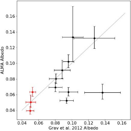
Figure 3: Comparison of albedos obtained using ALMA data to the rescaled albedos of Grav et al. (2012). The grey line is of slope 1, so that if the same result was found for an object in both analyses, it would fall on that line. The three objects used for emissivity calibration are shown in red.

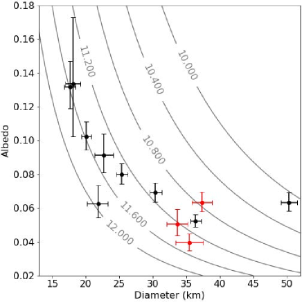
Figure 4: Diameter plotted against albedo for all objects modeled, with the three calibrators shown in red. Lines of constant absolute magnitude (Equation 2) are plotted in gray for values of absolute magnitude between 10 and 12. While it appears that diameter and albedo are anti-correlated, this apparent trend is driven mostly by the fact that for a given value of absolute magnitude, albedo and diameter can only fall along the indicated line. Because of the limited range of absolute magnitudes observed, it is unknown if small low albedo objects exists, though from the WISE data it is clear that large high albedo objects do not.

Based on the ZTF data, the spherical assumption for these objections is clearly incorrect. We perform simple experiments to determine if the derived albedos are systematically affected by this assumption. We create a series of ellipsoids with fixed albedos of 0.05, with random dimensions, observed at random angles, and with varying photometric functions, and we calculate the thermal flux density and absolute magnitude that would be measured for each object. We then insert these measurements into our thermal model and determine the albedo that would be inferred. We find an standard deviation of 6% between the derived values and the simulated values, and no systematic offset. We thus conclude that unknown elongation and viewing angle effects contribute an additional $\sim$6% uncertainty.

5 Discussion

Of the nine Jupiter Trojans for which WISE derived unusually high albedos, we find that four have ALMA-derived albedos less than 0.07, consistent with typical values in the larger population (Fig. 3). We have no reason to believe that these objects have changed since the time of the WISE observations, and the discrepancies between WISE assumed absolute magnitudes and those used here are uncorrelated with the magnitude (or sign) of the discrepancy between the WISE-derived albedos and those derived here. The higher S/N of the ALMA observations and the lower sensitivity to model assumptions suggests that the ALMA albedos are more reliable and that for some of these small objects WISE does indeed suffer from random and systematic uncertainties larger than the formal error bars.

Of the five remaining targets, four have ALMA-derived albedos consistent with those from WISE, while one has an even larger albedo than reported by WISE. With these observations completely independent and no reason to otherwise expect these objects to have high albedos, we regard the match between the ALMA and WISE albedos as strong confirmation of the higher-than-typical albedos of these objects. The two smallest objects, 13331 and 42168, have albedos nearly double that of the main Trojan population.

In our sample, albedos decrease systematically at smaller sizes (Fig. 4). Some of the decrease is a simple observational bias: objects with the same absolute magnitude but smaller sizes must necessarily have higher albedos. The absolute magnitudes of the majority of our sample are all between 10.8 and 11.8. The diameter vs. size of these objects must lie on a curve like shown in Figure 4. Small low albedo objects, if they exist, would have low absolute magnitudes and would not be included in our sample. Examination of the WISE results in Figure 1 suggests that such objects do indeed exist, though, again, unaccounted-for uncertainties could dominate at these small sizes in the WISE data. In contrast, large high albedo Trojans are unlikely to exist, as they would have been detected with high S/N in the WISE data.

Overall the ALMA results support the conclusion that a modest number of 15-25 km diameter Jupiter Trojans have albedos elevated above those of the general population. The sizes and numbers of these objects are consistent with the hypothesis that they are the expected larger diameter tail of recent collisional fragments. If this hypothesis is correct, we would expect a larger fraction of high albedo Trojans at smaller sizes. In addition, we would expect that these high albedo mid-sized Trojans could be the most likely location to find spectroscopic hints of the interior composition of Jupiter Trojans. Continued study of this population could yield critical insight into the formation location of these objects, and, by extension, into the dynamical history of the solar system.

Appendix A Asteroid Periodograms and Phased Lightcurves

The following figures reproduce Figure 2 for all objects for which periods were obtained.

References

- Bowell et al. (1989) Bowell, E., Hapke, B., Domingue, D., et al. 1989, in Asteroids II, ed. R. P. Binzel, T. Gehrels, & M. S. Matthews, 524–556
- Brown (2016) Brown, M. E. 2016, AJ, 152, 159, doi: 10.3847/0004-6256/152/6/159
- Brown et al. (2007) Brown, M. E., Barkume, K. M., Ragozzine, D., & Schaller, E. L. 2007, Nature, 446, 294, doi: 10.1038/nature05619
- Brunetto et al. (2006) Brunetto, R., Barucci, M. A., Dotto, E., & Strazzulla, G. 2006, ApJ, 644, 646, doi: 10.1086/503359
- Burnham & Darling (2004) Burnham, K. P., & Darling, D. R. 2004, Sociological Methods & Research, 33, 261, doi: 10.1177/0049124104268644
- de Elía & Brunini (2007) de Elía, G. C., & Brunini, A. 2007, A&A, 475, 375, doi: 10.1051/0004-6361:20077979
- De Luise et al. (2010) De Luise, F., Dotto, E., Fornasier, S., et al. 2010, Icarus, 209, 586, doi: 10.1016/j.icarus.2010.04.024
- Emery et al. (2011) Emery, J. P., Burr, D. M., & Cruikshank, D. P. 2011, AJ, 141, 25, doi: 10.1088/0004-6256/141/1/25
- Foreman-Mackey et al. (2013) Foreman-Mackey, D., Hogg, D. W., Lang, D., & Goodman, J. 2013, Publications of the Astronomical Society of the Pacific, 125, 306, doi: 10.1086/670067
- Fornasier et al. (2007) Fornasier, S., Dotto, E., Hainaut, O., et al. 2007, Icarus, 190, 622, doi: 10.1016/j.icarus.2007.03.033
- Francis et al. (2020) Francis, L., Johnstone, D., Herczeg, G., Hunter, T. R., & Harsono, D. 2020, The Astronomical Journal, 160, id.270
- French et al. (2015) French, L. M., Stephens, R. D., Coley, D., Wasserman, L. H., & Sieben, J. 2015, Icarus, 254, 1, doi: 10.1016/j.icarus.2015.03.026
- French et al. (2012) French, L. M., Stephens, R. D., Coley, D. R., Megna, R., & Wasserman, L. H. 2012, Minor Planet Bulletin, 39, 183. http://adsabs.harvard.edu/abs/2012MPBu...39..183F
- Grav et al. (2012) Grav, T., Mainzer, A. K., Bauer, J. M., Masiero, J. R., & Nugent, C. R. 2012, ApJ, 759, 49, doi: 10.1088/0004-637X/759/1/49
- Harris (1998) Harris, A. W. 1998, Icarus, 131, 291, doi: 10.1006/icar.1997.5865
- Harris et al. (2009) Harris, A. W., Mueller, M., Lisse, C. M., & Cheng, A. F. 2009, Icarus, 199, 86, doi: 10.1016/j.icarus.2008.09.004
- Jester et al. (2005) Jester, S., Schneider, D. P., Richards, G. T., et al. 2005, The Astronomical Journal, 130, 873, doi: 10.1086/432466
- Marsset et al. (2014) Marsset, M., Vernazza, P., Gourgeot, F., et al. 2014, Astronomy & Astrophysics, 568, L7, doi: 10.1051/0004-6361/201424105
- Marzari & Scholl (2002) Marzari, F., & Scholl, H. 2002, Icarus, 159, 328, doi: 10.1006/icar.2002.6904
- Morbidelli (2010) Morbidelli, A. 2010, Comptes Rendus Physique, 11, 651, doi: 10.1016/j.crhy.2010.11.001
- Morbidelli et al. (2005) Morbidelli, A., Levison, H. F., Tsiganis, K., & Gomes, R. 2005, Nature, 435, 462, doi: 10.1038/nature03540
- Muders et al. (2014) Muders, D., Wyrowski, F., Lightfoot, J., et al. 2014, in Astronomical Data Analysis Software and Systems XXIII, ed. N. Manset & P. Forshay, 383–386
- Ragozzine & Brown (2007) Ragozzine, D., & Brown, M. E. 2007, AJ, 134, 2160, doi: 10.1086/522334
- Ryan et al. (2017) Ryan, E. L., Sharkey, B. N. L., & Woodward, C. E. 2017, AJ, 153, 116, doi: 10.3847/1538-3881/153/3/116
- Schemel & Brown (2020) Schemel, M., & Brown, M. E. 2020, arXiv e-prints, 2011, arXiv:2011.01329. http://adsabs.harvard.edu/abs/2020arXiv201101329S
- Stephens et al. (2015) Stephens, R. D., Coley, D. R., & French, L. M. 2015, Minor Planet Bulletin, 42, 216. http://adsabs.harvard.edu/abs/2015MPBu...42R.216S
- Stephens et al. (2010) Stephens, R. D., Warner, B. D., & Harris, A. W. 2010, 42, 39.14. https://ui.adsabs.harvard.edu/abs/2010DPS....42.3914S
- Szabó et al. (2017) Szabó, G. M., Pál, A., Kiss, C., et al. 2017, A&A, 599, A44, doi: 10.1051/0004-6361/201629401
- Thompson et al. (2017) Thompson, A. R., Moran, J. M., & Swenson, G. W. 2017, Interferometry and Synthesis in Radio Astronomy, 3rd Edition (Switzerland: Springer Open)
- Thompson et al. (1987) Thompson, W. R., Murray, B. G. J. P. T., Khare, B. N., & Sagan, C. 1987, J. Geophys. Res., 92, 14933, doi: 10.1029/JA092iA13p14933
- Warner et al. (2011) Warner, B. D., Stephens, R. D., & Harris, A. W. 2011, Minor Planet Bulletin, 38, 172. https://ui.adsabs.harvard.edu/abs/2011MPBu...38..172W
- Wright et al. (2010) Wright, E. L., Eisenhardt, P. R. M., Mainzer, A. K., et al. 2010, AJ, 140, 1868, doi: 10.1088/0004-6256/140/6/1868