Rank-one Boolean tensor factorization and the multilinear polytope

Abstract

We consider the NP-hard problem of approximating a tensor with binary entries by a rank-one tensor, referred to as rank-one Boolean tensor factorization problem. We formulate this problem, in an extended space of variables, as the problem of minimizing a linear function over a highly structured multilinear set. Leveraging on our prior results regarding the facial structure of multilinear polytopes, we propose novel linear programming relaxations for rank-one Boolean tensor factorization. To analyze the performance of the proposed linear programs, we consider a semi-random corruption model for the input tensor. We first consider the original NP-hard problem and establish necessary and sufficient conditions for the recovery of the ground truth with high probability. Next, we obtain sufficient conditions under which the proposed linear programming relaxations recover the ground truth with high probability. Our theoretical results as well as numerical simulations indicate that certain facets of the multilinear polytope significantly improve the recovery properties of linear programming relaxations for rank-one Boolean tensor factorization.

Funding: A. Del Pia is partially funded by ONR grant N00014-19-1-2322.

Key words: Rank-one Boolean tensor factorization, multilinear polytope, linear programming relaxation, recovery guarantee, semi-random models

Mathematics Subject Classification: Primary: 90C10; secondary: 90C26, 90C57

1 Introduction

A tensor of order $N$ is an $N$-dimensional array. Factorizations of high-order tensors, i.e., $N\geq 3$, as products of low-rank matrices, have applications in signal processing, numerical linear algebra, computer vision, data mining, neuroscience, and elsewhere [31, 29, 46, 4]. We consider the problem of factorizing a high-order tensor with binary entries, henceforth, referred to as a binary tensor. Such problems arise in applications such as neuro-imaging, recommendation systems, topic modeling, and sensor network localization [45, 34, 41, 28]. In Boolean tensor factorization (BTF), the binary tensor is approximated by products of low rank binary matrices using Boolean algebra [35]. BTF is a very useful tool for analyzing binary tensors to discover latent factors from them [23, 39, 43, 44]. Furthermore, BTF produces more interpretable and sparser results than normal factorization methods [35]. BTF is NP-hard in general [25]; all existing methods to tackle this problem rely on heuristics and hence do not provide any guarantee on the quality of the solution [35, 23, 3, 39, 43].

In order to formally define BTF, we first introduce some notation. For an integer $n$, we denote by $[n]:=\{1,2,\dots,n\}$. All the tensors that we consider in this work have order three, meaning that each element of the tensor has three indices. Given a tensor ${\mathcal{W}}$, we denote its $(i,j,k)$th element by $w_{ijk}$. We denote by $\otimes$ the vector outer product. That is, if $x\in\mathbb{R}^{n}$, $y\in\mathbb{R}^{m}$, $z\in\mathbb{R}^{l}$, then ${\mathcal{W}}=x\otimes y\otimes z$ is a $n\times m\times l$ tensor defined by $w_{ijk}=x_{i}y_{j}z_{k}$, for $i\in[n]$, $j\in[m]$, $k\in[l]$. The Frobenius norm of a tensor ${\mathcal{W}}$, is defined as $\|{\mathcal{W}}\|:=\sqrt{\sum_{i,j,k}{w^{2}_{ijk}}}$. The rank (or Boolean rank) of a binary tensor ${\mathcal{W}}$ is the smallest integer $r$ such that there exist $3r$ binary vectors $x^{t},y^{t},z^{t}$, for $t\in[r]$, with

$${\mathcal{W}}=\bigvee^{r}_{t=1}(x^{t}\otimes y^{t}\otimes z^{t}),$$

where $\vee$ denotes the component-wise “or” operation. In particular, a binary tensor has rank one if it is the outer product of three binary vectors. Computing the Boolean rank of a binary tensor is NP-complete [26, 35]. Interestingly, unlike matrices, there exist $n\times m\times l$ binary tensors whose Boolean rank is larger than $\max\{n,m,l\}$. Indeed, a tight upper bound on the Boolean rank of a binary tensor is given by $\min\{nm,nl,ml\}$ [35].

Problem statement.

The rank-$r$ BTF is the problem of finding the closest rank-$r$ binary tensor to a given binary tensor. Precisely, we are given a $n\times m\times l$ binary tensor ${\mathcal{G}}$ and an integer $r$, and we seek $3r$ binary vectors $x^{t}\in\{0,1\}^{n}$, $y^{t}\in\{0,1\}^{m}$, $z^{t}\in\{0,1\}^{l}$, for all $t\in[r]$, that minimize

$$\Big{\lVert}{\mathcal{G}}-\bigvee^{r}_{t=1}x^{t}\otimes y^{t}\otimes z^{t}\Big{\rVert}^{2}.$$

In this paper, we focus on the simplest case of BTF; namely, the case with $r=1$, referred to as the rank-one BTF. This problem can be formulated as the following optimization problem:

$$\min\quad \Big{\|}{\mathcal{G}}-x\otimes y\otimes z\Big{\|}^{2}$$ (P)

$${\rm s.t.}\quad x\in\{0,1\}^{n},\ y\in\{0,1\}^{m},\ z\in\{0,1\}^{l}.$$

Rank-one BTF is NP-hard in general [35] and to this date no algorithm with theoretical guarantees is known for this problem. In this paper, we introduce novel linear programming (LP) relaxations with theoretical performance guarantees for rank-one BTF.

Recovery under a planted model.

It is widely accepted that worst-case guarantees for algorithms are often too pessimistic, as the input data in most real-world applications is highly structured. Motivated by this observation, a recent stream of research in mathematical optimization is focused on obtaining theoretical guarantees for various existing and new algorithms under reasonable stochastic models (see for example [1, 36, 32, 38, 18, 12, 11, 21, 5]). More specifically, in our context, under suitable generative models for the input, our goal is to obtain sufficient conditions under which the solution returned by the algorithm corresponds to the ground truth with high probability. Such conditions are often referred to as recovery guarantees [1, 36, 32, 18, 12, 11].

We now define our two stochastic models for rank-one BTF. First, we introduce the fully-random corruption model. Consider binary vectors $\bar{x}\in\{0,1\}^{n}$, $\bar{y}\in\{0,1\}^{m}$, $\bar{z}\in\{0,1\}^{l}$ and define the ground truth rank-one tensor $\bar{\mathcal{W}}=(w_{ijk}):=\bar{x}\otimes\bar{y}\otimes\bar{z}\in\{0,1\}^{n\times m\times l}$. Given $p\in[0,1]$, the noisy tensor ${\mathcal{G}}$ is constructed as follows: for each $(i,j,k)\in[n]\times[m]\times[l]$, $g_{ijk}$ is corrupted with probability $p$, i.e., $g_{ijk}:=1-\bar{x}_{i}\bar{y}_{j}\bar{z}_{k}$, and $g_{ijk}$ is not corrupted with probability $1-p$, i.e., $g_{ijk}:=\bar{x}_{i}\bar{y}_{j}\bar{z}_{k}$. This model has been used in [35, 39, 43] for conducting empirical analysis of some heuristics for BTF. It is well-understood that in case of fully-random models, heuristics may exploit the very special statistical properties of these models to succeed; properties that are not present in real-world instances (see for example [24]). To address this shortcoming, semi-random models have been introduced [24]; these models are generated by combining random and adversarial components. Semi-random models are often used to measure the “robustness” of algorithms as they better reflect real-world instances than fully-random models. It has been shown that, unlike some popular heuristics such as spectral methods that fail under semi-random models, optimization-based techniques such as semi-definite programming continue to work well under these models [24, 37, 42].

We now define the semi-random corruption model for rank-one BTF. In this model, first the noisy tensor $\mathcal{G}$ is constructed from the ground truth rank-one tensor $\bar{\mathcal{W}}$ according to the fully-random model. Then, an adversary modifies $\mathcal{G}$ by applying an arbitrary sequence of monotone transformations defined as follows:

• If an entry is 1 in $\bar{\mathcal{W}}$ and is 0 in $\mathcal{G}$, the adversary may revert to 1 the entry in $\mathcal{G}$;

• If an entry is 0 in $\bar{\mathcal{W}}$ and is 1 in $\mathcal{G}$, the adversary may revert to 0 the entry in $\mathcal{G}$.

It is important to note that while it seems the adversary makes helpful changes to the noisy tensor which should make the problem easier to solve, such changes break the special properties associated with the fully-random model and hence heuristics that highly rely on such unrealistic properties do not succeed in semi-random models.

Next, we define the term “recover the ground truth”. Consider an optimization problem for rank-one BTF. We say that this optimization problem recovers the ground truth, if the optimization problem has a unique optimal solution and it corresponds to the ground truth rank-one tensor $\bar{\mathcal{W}}$. In this paper, we study the following question: What is the maximum level of corruption, measured in terms of $p$, under which our optimization problems recover the ground truth with high probability? Throughout this paper, when we write that an event happens with high probability, we mean that the event happens with probability that goes to one, as $n,m,l\to\infty$. Our analysis is based on an important assumption that the optimization problem only receives the tensor ${\mathcal{G}}$ as input and does not have the knowledge of how it was generated; in particular, $p$ is not given to the optimization problem.

We say that an optimization problem is robust, if whenever it recovers the ground truth for an input tensor ${\mathcal{G}}$, then it also recovers the ground truth if an adversary modifies ${\mathcal{G}}$ by applying an arbitrary sequence of monotone transformations. As a consequence, if a robust optimization problem recovers the ground truth with high probability under the fully-random corruption model, then it also recovers the ground truth with high probability under the associated semi-random model. We prove that our proposed LP relaxations are robust. To the best of our knowledge, there exists no robust spectral method for rank-one BTF.

Denote by $r_{\bar{x}}$ (resp. $r_{\bar{y}}$, $r_{\bar{z}}$) the ratio of ones in $\bar{x}$ (resp. $\bar{y}$, $\bar{z}$) to the number of elements in $\bar{x}$ (resp. $\bar{y}$, $\bar{z}$). In this paper, we mainly focus on the case where $p$ is a constant, and we often consider the “dense regime,” in which $r_{\bar{x}}$, $r_{\bar{y}}$, and $r_{\bar{z}}$ are positive constants.

Our contribution.

In this paper, we introduce novel LP relaxations with theoretical performance guarantees for rank-one BTF. To construct the new LP relaxations, we first reformulate Problem (P), in an extended space of variables, as the problem of minimizing a linear function over a highly structured multilinear set [14]. This in turn enables us to leverage our previous results regarding the facial structure of the multilinear polytope [14, 16, 15, 17, 19], and develop strong LP relaxations for rank-one BTF. We investigate the recovery properties of the proposed LPs under the semi-random corruption model.

Clearly, any convex relaxation can recover the ground truth only if the original NP-hard problem succeeds in doing so. We start by establishing the recovery threshold for rank-one BTF under our two corruption models. Namely, we obtain necessary and sufficient conditions under which Problem (P) recovers the ground truth with high probability. In particular, our results imply that, under mild assumptions on the growth rate of $n,m,l$, Problem (P) recovers the ground truth with high probability if and only if $p<1/2$ (see Theorems 1 and 2).

We then study the recovery properties of our proposed LPs under the semi-random corruption model. We start by considering a simple LP relaxation for rank-one BTF, referred to as the standard LP, and obtain a recovery guarantee for it. Our result in particular implies if $r_{\bar{x}}=r_{\bar{y}}=r_{\bar{z}}$, under mild assumptions on the growth rate of $n,m,l$, the standard LP recovers the ground truth with high probability if $p<\frac{r_{\bar{w}}}{2(1+r_{\bar{w}})}$, where we define $r_{\bar{w}}:=r_{\bar{x}}r_{\bar{y}}r_{\bar{z}}$ (see Theorem 3). We refer to our strongest proposed LP relaxation as the complete LP. Since the theoretical analysis of the complete LP is rather complex, in this paper, as a starting point, we consider a relaxation of this LP, which we refer to as the flower LP. Roughly speaking, this intermediate LP is obtained by adding flower inequalities [15] to the standard LP. We prove that under mild assumptions on the growth rate of $n,m,l$, the flower LP recovers the ground truth with high probability if $p<\frac{r_{\bar{w}}}{1+2r_{\bar{w}}}$ (see Theorem 4). That is, utilizing a stronger LP relaxation results in an improvement of up to $33\%$ in the recovery threshold. Numerical experiments suggest that our recovery guarantees are fairly tight, and that the complete LP significantly outperforms the flower LP. Obtaining recovery guarantees for the complete LP is a subject of future research. We remark that all proposed LP relaxations can be solved efficiently both in theory (i.e., in polynomial time) and in practice.

Outline.

In Section 2, we introduce our LP relaxations for rank-one BTF. In Section 3 we present the statements of our main results. Preliminary numerical results are provided in Section 4. In Section 5, we prove our necessary and sufficient recovery conditions for rank-one BTF. In Sections 6 and 7, we prove our recovery guarantees for the standard LP and the flower LP, respectively. Finally, the proof of a technical result omitted from Section 2 is given in Section 8.

2 LP relaxations for rank-one BTF

In this section, we propose our novel LP relaxations for rank-one BTF. To this end, we first present an equivalent integer programming reformulation of Problem (P) in an extended space. Define

$$S_{0}:=\{(i,j,k)\in[n]\times[m]\times[l]:g_{ijk}=0\},\quad S_{1}:=\{(i,j,k)\in[n]\times[m]\times[l]:g_{ijk}=1\}.$$ (1)

Since ${\mathcal{G}},x,y,z$ are all binary valued, the objective function of Problem (P) can be written as

$$\Big{\|}{\mathcal{G}}-x\otimes y\otimes z\Big{\|}^{2}=\sum_{(i,j,k)\in S_{0}}{x_{i}y_{j}z_{k}}+\sum_{(i,j,k)\in S_{1}}{(1-x_{i}y_{j}z_{k})}.$$

Subsequently, we introduce auxiliary variables $w_{ijk}:=x_{i}y_{j}z_{k}$, for $i\in[n]$, $j\in[m]$, $k\in[l]$. It then follows that rank-one BTF can be equivalently written, in an extended space, as the problem of minimizing a linear function over a highly structured multilinear set:

$$\min\quad \sum_{(i,j,k)\in S_{0}}{w_{ijk}}+\sum_{(i,j,k)\in S_{1}}{(1-w_{ijk})}$$ (extP)

$${\rm s.t.}\quad w_{ijk}=x_{i}y_{j}z_{k},\qquad\forall i\in[n],j\in[m],k\in[l]$$

$$x\in\{0,1\}^{n},\ y\in\{0,1\}^{m},\ z\in\{0,1\}^{l}.$$

A simple LP relaxation of Problem (extP) can be obtained by replacing each multilinear term $w_{ijk}=x_{i}y_{j}z_{k}$, $x_{i},y_{j},z_{k}\in\{0,1\}$, by its convex hull [8]. Using the sign of the objective function coefficients, we remove a subset of constraints that are never active at an optimal solution to obtain:

$$\min\quad \sum_{(i,j,k)\in S_{0}}{w_{ijk}}+\sum_{(i,j,k)\in S_{1}}{(1-w_{ijk})}$$

$${\rm s.t.}\quad w_{ijk}\leq x_{i},\;w_{ijk}\leq y_{j},\;w_{ijk}\leq z_{k},\qquad\forall(i,j,k)\in S_{1}$$ (2)

$$w_{ijk}\geq 0,\;w_{ijk}\geq x_{i}+y_{j}+z_{k}-2,\qquad\forall(i,j,k)\in S_{0}$$ (3)

$$(x,y,z)\in[0,1]^{n+m+l}.$$ (4)

Throughout this paper, we refer to Problem (2) as the standard LP. In Sections 3 and 4, we investigate the effectiveness of this LP theoretically and numerically, respectively. Next, leveraging on our previous results regarding the facial structure of the convex hull of multilinear sets [14, 16, 15, 17, 19], we propose stronger LP relaxations for rank-one BTF.

2.1 Multilinear polytope of rank-one BTF

We start by providing a brief overview of the multilinear polytope. Subsequently, we propose new LP relaxations for rank-one BTF. Consider a hypergraph $G=(V,E)$, where $V$ is the set of nodes, and $E$ is the set of edges, where each edge is a subset of $V$ of cardinality at least two. The multilinear set ${\mathcal{S}}_{G}$ is defined as the set of binary points $(u,w)\in\{0,1\}^{V}\times\{0,1\}^{E}$ satisfying the collection of equations $w_{e}=\prod_{v\in e}{u_{v}}$, for all $e\in E$. The multilinear polytope $\text{MP}_{G}$ is defined as the convex hull of the multilinear set ${\mathcal{S}}_{G}$. The feasible region of Problem (extP) is a highly structured multilinear set and hence understanding the facial structure of its convex hull is key to constructing strong LP relaxations for rank-one BTF.

In [15, 17] we obtain sufficient conditions, in terms of acyclicity degree of the underlying hypergraph, under which the multilinear polytope has a compact extended formulation. As a byproduct, in these papers we introduce new classes of valid inequalities for the multilinear polytope. As we detail next, the proposed inequalities, namely, flower inequalities [15] and running intersection inequalities [17], turn out to be highly effective in constructing strong LP relaxations for rank-one BTF. For more theoretical results on the facial structure of the multilinear polytope, we refer the reader to [14, 16, 9, 6, 27, 13, 20].

Henceforth, we refer to the convex hull of the feasible region of Problem (extP) as the multilinear polytope of rank-one BTF, and we denote by $G^{\rm BT}$ its hypergraph. In particular, $G^{\rm BT}$ is a tripartite hypergraph: it has $n+m+l$ nodes, and each edge contains three nodes: one from the first $n$, one from the next $m$, and one from the last $l$. In the following, we consider a certain hypergraph, denoted by $\tilde{G}$, for which the corresponding multilinear polytope can be readily obtained. The interest in $\tilde{G}$ is twofold: first, its simplicity yields an elegant facet description; second, its special structure enables us to obtain a strong relaxation for the multilinear polytope of rank-one BTF.

Proposition 1.

Consider $\tilde{G}=(\tilde{V},\tilde{E})$ with $\tilde{V}=\{v_{1},\cdots,v_{6}\}$ and $\tilde{E}=\{e_{0},e_{1},e_{2},e_{3}\}$, where $e_{0}=\{v_{1},v_{3},v_{5}\}$, $e_{1}=\{v_{1},v_{3},v_{6}\}$, $e_{2}=\{v_{2},v_{3},v_{5}\}$, $e_{3}=\{v_{1},v_{4},v_{5}\}$. Then the facet description of $\text{MP}_{\tilde{G}}$ is given by:

$$w_{e}\leq u_{v},\qquad\forall e\in\tilde{E},\;\forall v\in e$$ (5)

$$w_{e}\geq 0,\;\quad\sum_{v\in e}{u_{v}}-w_{e}\leq 2,\qquad\forall e\in\tilde{E}$$ (6)

$$u_{v}\leq 1,\qquad\forall v\in\tilde{V}$$ (7)

$$u_{e_{0}\setminus e}+w_{e}-w_{e_{0}}\leq 1,\qquad\forall e\in\tilde{E}\setminus\{e_{0}\}$$ (8)

$$u_{e\setminus e_{0}}-w_{e}+w_{e_{0}}\leq 1,\qquad\forall e\in\tilde{E}\setminus\{e_{0}\}$$ (9)

$$-u_{e\cap e^{\prime}}+w_{e}+w_{e^{\prime}}-w_{e_{0}}\leq 0,\qquad\forall e\neq e^{\prime}\in\tilde{E}\setminus\{e_{0}\}$$ (10)

$$\sum_{v\in V}{u_{v}}-\sum_{e\in\tilde{E}\setminus\{e_{0}\}}{w_{e}}+w_{e_{0}}\leq 4.$$ (11)

Proof.

Follows from a direct check or by using a software such as PORTA [7]. ∎

To better understand the structure of $\text{MP}_{\tilde{G}}$, notice that inequalities (5)–(7) are of the form present in the standard LP. Inequalities (8), (9) are flower inequalities (see [15] for details), and inequalities (10) are running intersection inequalities (see [17] for details).

Since $\tilde{G}$ is a “building block” of $G^{\rm BT}$, we utilize the description of $\text{MP}_{\tilde{G}}$ in Proposition 1 to obtain a relaxation for the multilinear polytope of rank-one BTF. Formally, $\tilde{G}$ is a partial hypergraph of $G^{\rm BT}$, obtained by associating $u_{v_{1}},u_{v_{2}}$ to any two $x$ variables, $u_{v_{3}},u_{v_{4}}$ to any two $y$ variables, and $u_{v_{5}},u_{v_{6}}$ to any two $z$ variables. This in turn implies that inequalities defining $\text{MP}_{\tilde{G}}$ are also valid for the multilinear polytope of rank-one BTF.

While in general, flower inequalities and running intersection inequalities are not facet-defining for the multilinear polytope, as we show next, they define facets of the multilinear polytope of rank-one BTF. That is, we show that all facets of $\text{MP}_{\tilde{G}}$ defined in Proposition 1 are also facet-defining for $\text{MP}_{G^{\rm BT}}$.

Proposition 2.

All inequalities defining facets of $\text{MP}_{\tilde{G}}$ are facet-defining for $\text{MP}_{G^{\rm BT}}$ as well, once we associate $u_{v_{1}},u_{v_{2}}$ to any two $x$ variables, $u_{v_{3}},u_{v_{4}}$ to any two $y$ variables, and $u_{v_{5}},u_{v_{6}}$ to any two $z$ variables.

The proof of Proposition 2 relies on standard techniques and is given in Section 8. We remark that this result is highly nontrivial as it does not follow from any of the known lifting operations for the multilinear polytope [16], and is due to the fact that $G^{\rm BT}$ is a tripartite hypergraph.

2.2 New LP relaxations for rank-one BTF

Motivated by Propositions 1 and 2, we propose the following LP relaxation for rank-one BTF:

$$\min\quad \sum_{(i,j,k)\in S_{0}}{w_{ijk}}+\sum_{(i,j,k)\in S_{1}}{(1-w_{ijk})}$$

$${\rm s.t.}\quad w_{ijk}\leq x_{i},\;w_{ijk}\leq y_{j},\;w_{ijk}\leq z_{k},\qquad\forall(i,j,k)\in S_{1}$$

$$w_{ijk}\geq 0,\;w_{ijk}\geq x_{i}+y_{j}+z_{k}-2,\qquad\forall(i,j,k)\in S_{0}$$

$$w_{i^{\prime}jk}-w_{ijk}\leq 1-x_{i},\qquad\forall(i,j,k)\in S_{0},\;(i^{\prime},j,k)\in S_{1}$$

$$w_{ij^{\prime}k}-w_{ijk}\leq 1-y_{j},\qquad\forall(i,j,k)\in S_{0},\;(i,j^{\prime},k)\in S_{1}$$

$$w_{ijk^{\prime}}-w_{ijk}\leq 1-z_{k},\qquad\forall(i,j,k)\in S_{0},\;(i,j,k^{\prime})\in S_{1}$$

$$w_{ij^{\prime}k}+w_{ijk^{\prime}}-w_{ijk}\leq x_{i},\qquad\forall(i,j,k)\in S_{0},\;(i,j^{\prime},k)\in S_{1},\;(i,j,k^{\prime})\in S_{1}$$

$$w_{i^{\prime}jk}+w_{ijk^{\prime}}-w_{ijk}\leq y_{j},\qquad(i,j,k)\in S_{0},\;\forall(i^{\prime},j,k)\in S_{1},\;(i,j,k^{\prime})\in S_{1}$$

$$w_{i^{\prime}jk}+w_{ij^{\prime}k}-w_{ijk}\leq z_{k},\qquad\forall(i,j,k)\in S_{0},\;(i^{\prime},j,k)\in S_{1},\;(i,j^{\prime},k)\in S_{1}$$

$$x_{i}+x_{i^{\prime}}+y_{j}+y_{j^{\prime}}+z_{k}+z_{k^{\prime}}+w_{ijk}-w_{i^{\prime}jk}-w_{ij^{\prime}k}-w_{ijk^{\prime}}\leq 4,$$

$$\qquad\qquad\qquad\quad\forall(i^{\prime},j,k)\in S_{0},\;(i,j^{\prime},k)\in S_{0},\;(i,j,k^{\prime})\in S_{0},\;(i,j,k)\in S_{1}$$

$$(x,y,z)\in[0,1]^{n+m+l}.$$

We should remark that using the sign of the objective function coefficients, we have only kept a small subset of the facet-defining inequalities given in Proposition 1. In the remainder of the paper, we refer to Problem (2.2) as the complete LP. As we will show in Section 4, the complete LP is significantly stronger than the standard LP (2). However, it contains many more constraints: Problem (2) contains $\theta(|E|)$ constraints, whereas Problem (2.2) contains $O(|E|^{4})$ constraints, including $O(|E|^{2})$ flower inequalities and $O(|E|^{3})$ running intersection inequalities. Nonetheless, Problem (2.2) can be solved quite efficiently. In [19], we develop highly efficient separation algorithms for flower inequalities and running intersection inequalities. Utilizing these algorithms, one can develop an efficient customized LP solver for Problem (2.2).

Obtaining recovery guarantees for the complete LP is rather involved. To investigate the impact of the inequalities defining the complete LP in improving recovery properties of the standard LP, in this paper, we consider a specific relaxation of Problem (2.2), which we will refer as the flower LP.

$$\min\quad \sum_{(i,j,k)\in S_{0}}{w_{ijk}}+\sum_{(i,j,k)\in S_{1}}{(1-w_{ijk})}$$

$${\rm s.t.}\quad w_{ijk}\leq x_{i},\ w_{ijk}\leq y_{j},\ w_{ijk}\leq z_{k},\qquad\forall(i,j,k)\in S_{1}$$ (12)

$$w_{ijk}\geq 0,\quad w_{ijk}\geq x_{i}+y_{j}+z_{k}-2,\qquad\forall(i,j,k)\in S_{0}$$ (13)

$$w_{i^{\prime}jk}-w_{ijk}\leq 1-x_{i},\qquad\forall(i,j,k)\in S_{0},\;(i^{\prime},j,k)\in S_{1}$$ (14)

$$w_{ij^{\prime}k}-w_{ijk}\leq 1-y_{j},\qquad\forall(i,j,k)\in S_{0},\;(i,j^{\prime},k)\in S_{1}$$ (15)

$$w_{ijk^{\prime}}-w_{ijk}\leq 1-z_{k},\qquad\forall(i,j,k)\in S_{0},\;(i,j,k^{\prime})\in S_{1}$$ (16)

$$(x,y,z)\in[0,1]^{n+m+l}.$$ (17)

Due to its simpler formulation, Problem (2.2) is simpler to analyze than Problem (2.2) , yet, as we detail in Section 3, it significantly outperforms Problem (2) in recovering the ground truth.

Robustness of LP relaxations

We conclude this section by showing that the proposed LP relaxations of rank-one BTF are robust. We start by introducing some notation. Given binary vectors $\bar{x}\in\{0,1\}^{n}$, $\bar{y}\in\{0,1\}^{m}$, $\bar{z}\in\{0,1\}^{l}$, define $\bar{\mathcal{W}}=(w_{ijk}):=\bar{x}\otimes\bar{y}\otimes\bar{z}\in\{0,1\}^{n\times m\times l}$. Denote by ${\mathcal{G}}\in\{0,1\}^{n\times m\times l}$ a binary noisy tensor. Define:

$${\mathcal{P}}:=\{(i,j,k)\in[n]\times[m]\times[l]:\bar{x}_{i}=\bar{y}_{j}=\bar{z}_{k}=1\},$$

$${\mathcal{N}}:=\{(i,j,k)\in[n]\times[m]\times[l]:\bar{x}_{i}=0\;\lor\;\bar{y}_{j}=0\;\lor\;\bar{z}_{k}=0\},$$

$${\mathcal{T}}:=\{(i,j,k)\in[n]\times[m]\times[l]:g_{ijk}=\bar{x}_{i}\bar{y}_{j}\bar{z}_{k}\},$$

$${\mathcal{F}}:=\{(i,j,k)\in[n]\times[m]\times[l]:g_{ijk}=1-\bar{x}_{i}\bar{y}_{j}\bar{z}_{k}\}.$$

It then follows that

$$S_{0}=({\mathcal{T}}\cap{\mathcal{N}})\cup({\mathcal{F}}\cap{\mathcal{P}}),\qquad S_{1}=({\mathcal{T}}\cap{\mathcal{P}})\cup({\mathcal{F}}\cap{\mathcal{N}}),$$

where $S_{0},S_{1}$ are as defined in (1).

Lemma 1.

Problems (2), (2.2), and (2.2) are robust.

Proof.

We prove the statement for Problem (2). The proof for Problems (2.2) and (2.2) follows from a similar line of arguments. Let $\mathcal{G},\mathcal{G}^{\prime}\in\{0,1\}^{n\times m\times l}$ such that $\mathcal{G}^{\prime}$ can be obtained from $\mathcal{G}$ via a sequence of monotone transformations. We assume that $(\bar{x},\bar{y},\bar{z},\bar{\mathcal{W}})$ is the unique optimal solution of Problem (2) associated with tensor ${\mathcal{G}}$. We show that $(\bar{x},\bar{y},\bar{z},\bar{\mathcal{W}})$ is the unique optimal solution of Problem (2) associated with tensor ${\mathcal{G}}^{\prime}$ as well.

Define ${\mathcal{T}}^{\prime}:=\{(i,j,k)\in[n]\times[m]\times[l]:g^{\prime}_{ijk}=\bar{x}_{i}\bar{y}_{j}\bar{z}_{k}\}$ and define $Q:={\mathcal{T}}^{\prime}\setminus{\mathcal{T}}$. Notice that by definition ${\mathcal{T}}^{\prime}\supset{\mathcal{T}}$. Denote by LP1, Problem (2) associated with tensor ${\mathcal{G}}$ and denote by LP2, Problem (2) associated with tensor ${\mathcal{G}}^{\prime}$. Since $(\bar{x},\bar{y},\bar{z},\bar{\mathcal{W}})$ is the unique optimal solution of LP1, the optimal value of this LP is given by $|{\mathcal{F}}|$. Moreover, $(\bar{x},\bar{y},\bar{z},\bar{\mathcal{W}})$ is a feasible solution of LP2 with the objective value equal to $|{\mathcal{F}}|-|Q|$. Suppose that $(\bar{x},\bar{y},\bar{z},\bar{\mathcal{W}})$ is not the unique optimal solution of LP2; then there exists a solution $(\tilde{x},\tilde{y},\tilde{z},\tilde{\mathcal{W}})$ different from $(\bar{x},\bar{y},\bar{z},\bar{\mathcal{W}})$ whose objective value is less that or equal to $|{\mathcal{F}}|-|Q|$. Define $S^{\prime}_{0}:=\{(i,j,k)\in[n]\times[m]\times[l]:g^{\prime}_{ijk}=0\}=({\mathcal{T}}^{\prime}\cap{\mathcal{N}})\cup({\mathcal{F}}^{\prime}\cap{\mathcal{P}})$ and $S^{\prime}_{1}:=\{(i,j,k)\in[n]\times[m]\times[l]:g^{\prime}_{ijk}=1\}=({\mathcal{T}}^{\prime}\cap{\mathcal{P}})\cup({\mathcal{F}}^{\prime}\cap{\mathcal{N}})$, where ${\mathcal{F}}^{\prime}={\mathcal{F}}\cup Q$. Let us examine the objective value $\tilde{f}$ of LP2 at $(\tilde{x},\tilde{y},\tilde{z},\tilde{\mathcal{W}})$:

$$\tilde{f}= \sum_{(i,j,k){\mathcal{S}}^{\prime}_{0}}{\tilde{w}_{ijk}}+\sum_{(i,j,k){\mathcal{S}}^{\prime}_{1}}{(1-\tilde{w}_{ijk})}$$ (18)

$$= \sum_{(i,j,k)\in{\mathcal{S}}_{0}}{\tilde{w}_{ijk}}+\sum_{(i,j,k)\in Q\cap{\mathcal{N}}}{\tilde{w}_{ijk}}-\sum_{(i,j,k)\in Q\cap{\mathcal{P}}}{\tilde{w}_{ijk}}+\sum_{(i,j,k)\in{\mathcal{S}}_{1}}{(1-\tilde{w}_{ijk})}+\sum_{(i,j,k)\in Q\cap{\mathcal{P}}}{(1-\tilde{w}_{ijk})}$$

$$-\sum_{(i,j,k)\in Q\cap{\mathcal{N}}}{(1-\tilde{w}_{ijk})}$$

$$= \sum_{(i,j,k)\in{\mathcal{S}}_{0}}{\tilde{w}_{ijk}}+\sum_{(i,j,k)\in{\mathcal{S}}_{1}}{(1-\tilde{w}_{ijk})}-\Big{(}\sum_{(i,j,k)\in Q\cap{\mathcal{P}}}{(2\tilde{w}_{ijk}-1)}-\sum_{(i,j,k)\in Q\cap{\mathcal{N}}}{(2\tilde{w}_{ijk}-1)}\Big{)}$$

$$\leq |F|-|Q|.$$ (19)

Moreover, since $0\leq\tilde{w}_{ijk}\leq 1$ for all $(i,j,k)\in[n]\times[m]\times[l]$, we have:

$$\sum_{(i,j,k)\in Q\cap{\mathcal{P}}}{(2\tilde{w}_{ijk}-1)}-\sum_{(i,j,k)\in Q\cap{\mathcal{N}}}{(2\tilde{w}_{ijk}-1)}\leq|Q\cap{\mathcal{P}}|+|Q\cap{\mathcal{N}}|=|Q|.$$ (20)

From (18) and (20) it follows that

$$\sum_{(i,j,k)\in{\mathcal{S}}_{0}}{\tilde{w}_{ijk}}+\sum_{(i,j,k)\in{\mathcal{S}}_{1}}{(1-\tilde{w}_{ijk})}\leq|F|,$$ (21)

which contradicts with the assumption that $(\bar{x},\bar{y},\bar{z},\bar{\mathcal{W}})$ is the unique optimal solution of LP1. Therefore, $(\bar{x},\bar{y},\bar{z},\bar{\mathcal{W}})$ is the unique optimal solution of LP2 as well and this completes the proof. ∎

In particular, Lemma 1 enables us to establish recovery under the semi-random corruption model by proving recovery under the simpler fully-random corruption model.

3 Main results

In this section, we summarize the main results of this paper. The proofs are deferred to Sections 5, 6 and 7.

3.1 Recovery conditions for rank-one BTF

We start by characterizing the corruption range, in terms of $p$, for which rank-one BTF can recover the ground truth with high probability. Such conditions serve as a reference point for assessing the effectiveness of our LP relaxations. Our results for Rank-one BTF essentially indicate that Problem (P) recovers the ground truth with high probability if and only if $p<1/2$. These results can be seen as tight, since in the fully-random model for $p=1/2$, each entry of the noisy tensor $\mathcal{G}$ is zero or one with equal probability, no matter what the original ground truth rank-one tensor $\bar{\mathcal{W}}$ is.

First, we present necessary conditions under which Problem (P) recovers the ground truth. Note that, this result holds already for the simpler fully-random corruption model.

Theorem 1 (Necessary conditions for recovery).

Consider the fully-random corruption model. If $p\geq 1/2$, then the probability that Problem (P) recovers the ground truth is at most $1/2$. Furthermore, if $r_{\bar{x}},r_{\bar{y}},r_{\bar{z}},p$ are positive constants and $p>1/2$, then with high probability Problem (P) does not recover the ground truth.

Next, we give sufficient conditions under which Problem (P) recovers the ground truth with high probability. This result holds for the more general semi-random corruption model.

Theorem 2 (Sufficient conditions for recovery).

Consider the semi-random corruption model. Assume that $r_{\bar{x}},r_{\bar{y}},r_{\bar{z}}$ are positive constants and

$$\lim_{n,m,l\to\infty}\frac{n+m+l}{\min\{nm,nl,ml\}}=0.$$ (22)

If $p$ is a constant satisfying $p<1/2$, then Problem (P) recovers the ground truth with high probability.

Proofs of the above theorems are given in Section 5. In fact, in Section 5, we also present more general conditions for recovery in which we do not assume that $r_{\bar{x}},r_{\bar{y}},r_{\bar{z}},p$ are constants (see Propositions 3 and 4).

Remark 1.

The limit assumption (22) in Theorem 2 is not too restrictive. Consider $m$ and $l$ as functions of $n$, i.e., $m=m(n)$ and $l=l(n)$. Furthermore, assume that $m(n)$ grows faster than $n$ and that $l(n)$ grows faster than $m(n)$, i.e. $n\in O(m(n))$, $m(n)\in O(l(n))$. Then assumption (22) is satisfied if $l(n)\in o(nm(n))$. Intuitively, sufficient conditions of Theorem 2 require that the functions $m(n)$ and $l(n)$ grow similarly as $n$ increases. Two simple examples of functions that satisfy these assumptions are: (2.i). $m(n),l(n)\in\Theta(n^{k})$, for any positive integer $k$; (2.ii). $m(n),l(n)\in\Theta(\exp(n))$. An example of functions that do not satisfy the assumptions of Theorem 2 is: $m(n)\in\Theta(n^{k})$ and $l(n)\in\Theta(n^{k+1})$, for any positive integer $k$.

3.2 Recovery guarantees for the standard LP

Next, we present recovery guarantees for the standard LP; namely, Problem (2). In particular, we obtain a sufficient condition in terms of $p,r_{\bar{x}},r_{\bar{y}},r_{\bar{z}}$ under which the standard LP recovers the ground truth with high probability.

Theorem 3.

Consider the semi-random corruption model. Assume that $r_{\bar{x}},r_{\bar{y}},r_{\bar{z}}$ are positive constants, and without loss of generality, assume $r_{\bar{x}}\geq r_{\bar{y}}\geq r_{\bar{z}}$. Assume that, as $n,m,l\to\infty$, we have $n\exp(-m)$, $n\exp(-l)$, $m\exp(-n)$, $m\exp(-l)$, $l\exp(-n)$, $l\exp(-m)\to 0$. If $p$ is a constant satisfying

$$p<\frac{r_{\bar{x}}r_{\bar{y}}r_{\bar{z}}}{2(1+r_{\bar{x}}r_{\bar{y}}r_{\bar{z}})+\delta},$$ (23)

where

$$\delta:=\frac{1}{2}r_{\bar{x}}r_{\bar{y}}+\frac{1}{2}r_{\bar{x}}r_{\bar{z}}-r_{\bar{y}}r_{\bar{z}}+r_{\bar{x}}-\frac{1}{2}r_{\bar{y}}-\frac{1}{2}r_{\bar{z}}\geq 0,$$

then Problem (2) recovers the ground truth with high probability.

Note that $\delta\geq 0$ since the assumption $r_{\bar{x}}\geq r_{\bar{y}}\geq r_{\bar{z}}$ implies that $r_{\bar{x}}r_{\bar{y}}+r_{\bar{x}}r_{\bar{z}}\geq 2r_{\bar{y}}r_{\bar{z}}$ and $2r_{\bar{x}}\geq r_{\bar{y}}+r_{\bar{z}}$, and these inequalities are satisfied tightly only if $r_{\bar{x}}=r_{\bar{y}}=r_{\bar{z}}$. Now suppose that the ground truth satisfies $r_{\bar{x}}=r_{\bar{y}}=r_{\bar{z}}$, and denote by $r_{\bar{w}}$ the tensor density; i.e., $r_{\bar{w}}:=r_{\bar{x}}r_{\bar{y}}r_{\bar{z}}$. We then obtain the following corollary of Theorem 3:

Corollary 1.

Consider the semi-random corruption model. Suppose that $r_{\bar{x}},r_{\bar{y}},r_{\bar{z}}$ are positive constants satisfying $r_{\bar{x}}=r_{\bar{y}}=r_{\bar{z}}$ and let $r_{\bar{w}}:=r_{\bar{x}}r_{\bar{y}}r_{\bar{z}}$. Assume that, as $n,m,l\to\infty$, we have $n\exp(-m)$, $n\exp(-l)$, $m\exp(-n)$, $m\exp(-l)$, $l\exp(-n)$, $l\exp(-m)\to 0$. If $p$ is a constant satisfying

$$p<\frac{r_{\bar{w}}}{2(1+r_{\bar{w}})},$$

then Problem (2) recovers the ground truth with high probability.

The proof of Theorem 3 is given in Section 6. To prove this result, we first obtain a deterministic sufficient condition for recovery (see Propositions 6 and 8). Then, using the deterministic condition together with Lemma 1, we derive a recovery guarantee under the semi-random corruption model.

Remark 2.

The limit assumptions in Theorem 3 are not too restrictive. Consider $m$ and $l$ as functions of $n$, i.e., $m=m(n)$ and $l=l(n)$. Two simple examples of functions that satisfy the assumptions of Theorem 3 are: (3.i). $m(n)\in\Theta(n^{h})$ and $l(n)\in\Theta(n^{k})$, for positive integers $h,k$; (3.ii). $m(n),l(n)\in\Theta(\exp(n/2))$. It is important to note that the limit assumptions in Theorem 3 are not comparable to those in Theorem 2. In particular, (3.i) contains as special case the example given in Remark 1 (i.e., $m(n)\in\Theta(n^{k})$, $l(n)\in\Theta(n^{k+1})$) that does not satisfy assumption (22). On the other hand, example (2.ii) does not satisfy the limit assumptions in Theorem 3.

3.3 Recovery guarantees for the flower LP

Next, we present recovery a guarantee for the flower LP; namely, Problem (2.2):

Theorem 4.

Consider the semi-random corruption model. Assume that $r_{\bar{x}},r_{\bar{y}},r_{\bar{z}}$ are positive constants and let $r_{\bar{w}}:=r_{\bar{x}}r_{\bar{y}}r_{\bar{z}}$. Assume that, as $n,m,l\to\infty$, we have $nml\exp(-n)$, $nml\exp(-m)$, $nml\exp(-l)\to 0$. If $p$ is a constant satisfying

$$p<\frac{r_{\bar{w}}}{1+2r_{\bar{w}}},$$ (24)

then Problem (2.2) recovers the ground truth with high probability.

The proof of Theorem 4 is given in Section 7. Our proof scheme is similar to that of Theorem 3: we first obtain a deterministic sufficient condition for recovery (see Propositions 9 and 10); next we consider the semi-random corruption model.

Remark 3.

The limit assumptions in Theorem 4 are not too restrictive, even though they are stronger than the limit assumptions in Theorem 3. Consider $m$ and $l$ as functions of $n$, i.e., $m=m(n)$ and $l=l(n)$. A simple example of functions that satisfies the assumptions of Theorem 4 is example (3.i) of Remark 2. On the other hand, example (3.ii) of Remark 2 does not satisfy the assumptions of Theorem 3. An example of functions that satisfies the assumptions in all Theorems 2, 3 and 4 is example (2.i) of Remark 1.

The recovery thresholds of the two LP relaxations for rank-one BTF together with rank-one BTF are depicted in Figure 1: the addition of flower inequalities significantly improves the recovery properties of the LP relaxation.

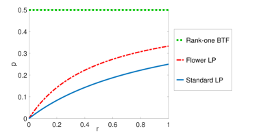
Figure 1: Comparison of the recovery threshold for two LP relaxations of Rank-one BTF under the semi-random corruption model as given by Corollary 1 and Theorem 4.

We conclude this section by observing that the parameter $p$ is not an input to our LP relaxation schemes. Hence, the knowledge of such parameter is not necessary for our recovery guarantees, which is an important and desirable property.

4 Numerical experiments

In this section, we conduct a preliminary numerical study to compare the recovery properties of the proposed LP relaxations for rank-one BTF. A comprehensive computational study that includes real data sets from the literature is a topic of future research.

We consider three LP relaxations for rank-one BTF: (i) the standard LP, defined by Problem (2), (ii) the flower LP, defined by Problem (2.2), and (iii) the complete LP, defined by Problem (2.2). We generate the input tensor ${\mathcal{G}}$ according to the fully-random corruption model defined before. For our numerical experiments we set $n=m=l=15$, $r_{\bar{w}}\in[0:0.04:1.0]$, and $p\in[0:0.01:0.5]$. For each fixed pair $(r_{\bar{w}},p)$, we run 40 random trials. We then count the number of times each LP relaxation recovers the ground truth. Dividing by the number of trials, we obtain the empirical rate of recovery. All experiments are performed on the NEOS server [10] and all LPs are solved with GAMS/CPLEX [30]. Results are shown in Figure 2; as can be seen from Figures 2(a) and 2(b), our recovery guarantees given by Theorems 3 and 4 are fairly tight, and we conjecture that these conditions are necessary for recovery as well. Moreover, Figure 2(c) indicates that the complete LP significantly outperforms the flower LP and hence understanding its recovery properties is an important topic of future research.

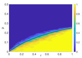
(a) Standard LP 

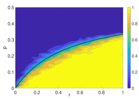
(b) Flower LP 

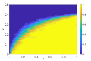
(c) Complete LP 

Figure 2: The empirical rate of recovery for LP relaxations of Rank-one BTF under the fully-random corruption model. The black curves in Figures 2(a) and 2(b) correspond to the recovery guarantees given by Corollary 1 and Theorem 4, respectively.

Finally, we would like to remark that while the recovery threshold of the original NP-hard problem is independent of the density of the input tensor, our theoretical and numerical results indicate that for all considered LP relaxations of rank-one BTF, the recovery threshold improves as the tensor density increases. This is indeed in agreement with several studies on graph problems, discovering that LP relaxations perform better on denser graphs (see for example [40, 2, 18]).

5 Recovery proofs for rank-one BTF

The main goal of this section is to prove Theorems 1 and 2. We start by introducing some notation that will be used in this section. Let $(\bar{x},\bar{y},\bar{z})\in\{0,1\}^{n+m+l}$. Like in the corruption models, we denote by $r_{\bar{x}}$ (resp. $r_{\bar{y}}$, $r_{\bar{z}}$) the ratio of ones in $\bar{x}$ (resp. $\bar{y}$, $\bar{z}$) to the number of elements in $\bar{x}$ (resp. $\bar{y}$, $\bar{z}$). For every $(x,y,z)\in\{0,1\}^{n+m+l}$, we denote by

$$\Delta_{(x,y,z)}:=\{(i,j,k)\in[n]\times[m]\times[l]\mid\bar{x}_{i}\bar{y}_{j}\bar{z}_{k}\neq x_{i}y_{j}z_{k}\},\qquad\delta_{(x,y,z)}:=\lvert\Delta_{(x,y,z)}\rvert.$$

For every $(x,y,z)\in\{0,1\}^{n+m+l}$ and every $s,t\in\{0,1\}$, we define the following sets:

$$X_{st}:=\{i\in[n]\mid\bar{x}_{i}=s,\,x_{i}=t\},\ Y_{st}:=\{j\in[m]\mid\bar{y}_{j}=s,\,y_{j}=t\},\ Z_{st}:=\{k\in[l]\mid\bar{z}_{k}=s,\,z_{k}=t\}.$$

For every $(x,y,z)\in\{0,1\}^{n+m+l}$, we denote by $\operatorname{obj}(x,y,z)$ the objective function of (P). Such function is explicitly given by

$$\operatorname{obj}(x,y,z):=\Big{\|}{\mathcal{G}}-x\otimes y\otimes z\Big{\|}^{2}=\sum_{\begin{subarray}{c}i\in[n],\ j\in[m],\ k\in[l]:\\ g_{ijk}=0\end{subarray}}{x_{i}y_{j}z_{k}}+\sum_{\begin{subarray}{c}i\in[n],\ j\in[m],\ k\in[l]:\\ g_{ijk}=1\end{subarray}}{(1-x_{i}y_{j}z_{k})},$$

and it gives the number of triples $(i,j,k)\in[n]\times[m]\times[l]$ for which $x_{i}y_{j}z_{k}\neq g_{ijk}$. In the remainder of the paper we also denote by $\operatorname{\mathbb{P}}[A]$ the probability of an event $A$, and by $\operatorname{\mathbb{E}}[X]$ the expected value of a random variable $X$.

5.1 Some useful lemmas

Next, we present two lemmas that will be useful in our analysis. In Lemma 2, we study the quantity $\delta_{(x,y,z)}$ and provide a lower bound.

Lemma 2.

Let $(\bar{x},\bar{y},\bar{z})\in\{0,1\}^{n+m+l}$.

1. For every $(x,y,z)\in\{0,1\}^{n+m+l}$, we have

   $$\delta_{(x,y,z)} =\lvert X_{11}\rvert\lvert Y_{11}\rvert\lvert Z_{10}\rvert+\lvert X_{11}\rvert\lvert Y_{10}\rvert\lvert Z_{11}\rvert+\lvert X_{10}\rvert\lvert Y_{11}\rvert\lvert Z_{11}\rvert+\lvert X_{11}\rvert\lvert Y_{10}\rvert\lvert Z_{10}\rvert+\lvert X_{10}\rvert\lvert Y_{11}\rvert\lvert Z_{10}\rvert$$

   $$\,+\lvert X_{10}\rvert\lvert Y_{10}\rvert\lvert Z_{11}\rvert+\lvert X_{10}\rvert\lvert Y_{10}\rvert\lvert Z_{10}\rvert+\lvert X_{11}\rvert\lvert Y_{11}\rvert\lvert Z_{01}\rvert+\lvert X_{11}\rvert\lvert Y_{01}\rvert\lvert Z_{11}\rvert+\lvert X_{01}\rvert\lvert Y_{11}\rvert\lvert Z_{11}\rvert$$

   $$\,+\lvert X_{11}\rvert\lvert Y_{01}\rvert\lvert Z_{01}\rvert+\lvert X_{01}\rvert\lvert Y_{11}\rvert\lvert Z_{01}\rvert+\lvert X_{01}\rvert\lvert Y_{01}\rvert\lvert Z_{11}\rvert+\lvert X_{01}\rvert\lvert Y_{01}\rvert\lvert Z_{01}\rvert.$$

2. For every $(x,y,z)\in\{0,1\}^{n+m+l}$ such that $(x,y,z)\neq(\bar{x},\bar{y},\bar{z})$, we have

   $$\delta_{(x,y,z)}\geq\min\{r_{\bar{x}}nr_{\bar{y}}m,r_{\bar{x}}nr_{\bar{z}}l,r_{\bar{y}}mr_{\bar{z}}l\}.$$

Proof.

(i). Let $(x,y,z)\in\{0,1\}^{n+m+l}$. We have

$$\Delta_{(x,y,z)} =\{(i,j,k)\in[n]\times[m]\times[l]\mid\bar{x}_{i}\bar{y}_{j}\bar{z}_{k}=1,x_{i}y_{j}z_{k}=0\}$$

$$\quad\cup\{(i,j,k)\in[n]\times[m]\times[l]\mid\bar{x}_{i}\bar{y}_{j}\bar{z}_{k}=0,x_{i}y_{j}z_{k}=1\},$$

where the union is disjoint. Thus,

$$\delta_{(x,y,z)} =(\lvert X_{11}\rvert\lvert Y_{11}\rvert\lvert Z_{10}\rvert+\lvert X_{11}\rvert\lvert Y_{10}\rvert\lvert Z_{11}\rvert+\lvert X_{10}\rvert\lvert Y_{11}\rvert\lvert Z_{11}\rvert+\lvert X_{11}\rvert\lvert Y_{10}\rvert\lvert Z_{10}\rvert+\lvert X_{10}\rvert\lvert Y_{11}\rvert\lvert Z_{10}\rvert$$

$$\,+\lvert X_{10}\rvert\lvert Y_{10}\rvert\lvert Z_{11}\rvert+\lvert X_{10}\rvert\lvert Y_{10}\rvert\lvert Z_{10}\rvert)+(\lvert X_{11}\rvert\lvert Y_{11}\rvert\lvert Z_{01}\rvert+\lvert X_{11}\rvert\lvert Y_{01}\rvert\lvert Z_{11}\rvert+\lvert X_{01}\rvert\lvert Y_{11}\rvert\lvert Z_{11}\rvert$$

$$\,+\lvert X_{11}\rvert\lvert Y_{01}\rvert\lvert Z_{01}\rvert+\lvert X_{01}\rvert\lvert Y_{11}\rvert\lvert Z_{01}\rvert+\lvert X_{01}\rvert\lvert Y_{01}\rvert\lvert Z_{11}\rvert+\lvert X_{01}\rvert\lvert Y_{01}\rvert\lvert Z_{01}\rvert).$$

(ii). Let $(x,y,z)\in\{0,1\}^{n+m+l}$ such that $(x,y,z)\neq(\bar{x},\bar{y},\bar{z})$. From (i), we have

$$\delta_{(x,y,z)} \geq\lvert X_{10}\rvert\lvert Y_{11}\rvert\lvert Z_{11}\rvert+\lvert X_{10}\rvert\lvert Y_{11}\rvert\lvert Z_{10}\rvert+\lvert X_{10}\rvert\lvert Y_{10}\rvert\lvert Z_{11}\rvert+\lvert X_{10}\rvert\lvert Y_{10}\rvert\lvert Z_{10}\rvert$$

$$=\lvert X_{10}\rvert(\lvert Y_{11}\rvert+\lvert Y_{10}\rvert)(\lvert Z_{11}\rvert+\lvert Z_{10}\rvert)=\lvert X_{10}\rvert r_{\bar{y}}mr_{\bar{z}}l.$$

Thus, if we assume $\lvert X_{10}\rvert\geq 1$, we obtain $\delta_{(x,y,z)}\geq r_{\bar{y}}mr_{\bar{z}}l$ and we are done. Symmetrically, if we assume $\lvert Y_{10}\rvert\geq 1$, we obtain $\delta_{(x,y,z)}\geq r_{\bar{x}}nr_{\bar{z}}l$ and we are done. Symmetrically, if we assume $\lvert Z_{10}\rvert\geq 1$, we obtain $\delta_{(x,y,z)}\geq r_{\bar{x}}nr_{\bar{y}}m$ and we are done.

Thus we now assume $X_{10}=Y_{10}=Z_{10}=\emptyset$, which implies $\lvert X_{11}\rvert=r_{\bar{x}}n$, $\lvert Y_{11}\rvert=r_{\bar{y}}m$, and $\lvert Z_{11}\rvert=r_{\bar{z}}l$. Since $(x,y,z)\neq(\bar{x},\bar{y},\bar{z})$, at least one of the sets $X_{01}$, $Y_{01}$, $Z_{01}$ is nonempty. If $\lvert X_{01}\rvert\geq 1$, then from (i) we have

$$\delta_{(x,y,z)}\geq\lvert X_{01}\rvert\lvert Y_{11}\rvert\lvert Z_{11}\rvert\geq\lvert Y_{11}\rvert\lvert Z_{11}\rvert=r_{\bar{y}}mr_{\bar{z}}l$$

and we are done. Symmetrically, if $\lvert Y_{01}\rvert\geq 1$, we obtain $\delta_{(x,y,z)}\geq r_{\bar{x}}nr_{\bar{z}}l$ and we are done. Symmetrically, if $\lvert Z_{01}\rvert\geq 1$, we obtain $\delta_{(x,y,z)}\geq r_{\bar{x}}nr_{\bar{y}}m$ and we are done. ∎

In Lemma 3, we study the probabilities that a vector $(x,y,z)\in\{0,1\}^{n+m+l}$ has value $\operatorname{obj}(x,y,z)$ smaller or larger than $\operatorname{obj}(\bar{x},\bar{y},\bar{z})$ in the fully-random corruption model.

Lemma 3.

Consider the fully-random corruption model. Let $(x,y,z)\in\{0,1\}^{n+m+l}$ such that $(x,y,z)\neq(\bar{x},\bar{y},\bar{z})$ and let $\delta:=\delta_{(x,y,z)}$. Then we have:

1. $\operatorname{\mathbb{P}}[\operatorname{obj}(x,y,z)>\operatorname{obj}(\bar{x},\bar{y},\bar{z})]=\sum_{\ell=0}^{\lceil\delta/2\rceil-1}\binom{\delta}{\ell}p^{\ell}(1-p)^{\delta-\ell}.$

2. If $p\leq 1/2$, then $\operatorname{\mathbb{P}}[\operatorname{obj}(x,y,z)\leq\operatorname{obj}(\bar{x},\bar{y},\bar{z})]\leq\exp\left(-2\delta(1/2-p)^{2}\right).$

3. If $p\geq 1/2$, then $\operatorname{\mathbb{P}}[\operatorname{obj}(x,y,z)\geq\operatorname{obj}(\bar{x},\bar{y},\bar{z})]\leq\exp\left(-2\delta(p-1/2)^{2}\right).$

Proof.

(i) In the case $\delta=0$, we have $\operatorname{obj}(x,y,z)=\operatorname{obj}(\bar{x},\bar{y},\bar{z})$ and the sum in the statement is vacuous, thus we are done. Assume now $\delta>0$. Note that $\operatorname{obj}(x,y,z)>\operatorname{obj}(\bar{x},\bar{y},\bar{z})$ if and only if strictly less than half of the $(i,j,k)\in\Delta_{(x,y,z)}$ are corrupted. We obtain

$$\operatorname{\mathbb{P}}[\operatorname{obj}(x,y,z)>\operatorname{obj}(\bar{x},\bar{y},\bar{z})]=\sum_{\ell=0}^{\lceil\delta/2\rceil-1}\binom{\delta}{\ell}p^{\ell}(1-p)^{\delta-\ell}.$$

(ii) In the case $\delta=0$, we have $\exp\left(-2\delta(1/2-p)^{2}\right)=\exp(0)=1$, thus we are done. Assume now $\delta>0$. Note that $\operatorname{obj}(x,y,z)\leq\operatorname{obj}(\bar{x},\bar{y},\bar{z})$ if and only if at least half of the $(i,j,k)\in\Delta_{(x,y,z)}$ are corrupted. For every $(i,j,k)\in\Delta_{(x,y,z)}$, let $B_{(i,j,k)}$ be the Bernoulli random variable defined by $B_{(i,j,k)}:=1$, if $(i,j,k)$ is corrupted, and $B_{(i,j,k)}:=0$, if $(i,j,k)$ is not corrupted. Consider the Binomial random variable

$$S_{\delta}:=\sum_{(i,j,k)\in\Delta_{(x,y,z)}}B_{(i,j,k)}.$$

We obtain that $\operatorname{obj}(x,y,z)\leq\operatorname{obj}(\bar{x},\bar{y},\bar{z})$ if and only if $S_{\delta}\geq\delta/2$. Note that $\operatorname{\mathbb{E}}[S_{\delta}]=\delta p$, thus

$$\operatorname{\mathbb{P}}[\operatorname{obj}(x,y,z)\leq\operatorname{obj}(\bar{x},\bar{y},\bar{z})]=\operatorname{\mathbb{P}}[S_{\delta}\geq\delta/2]=\operatorname{\mathbb{P}}[S_{\delta}-\operatorname{\mathbb{E}}[S_{\delta}]\geq\delta(1/2-p)].$$

By assumption $p\leq 1/2$ and $\delta>0$, thus in particular $\delta(1/2-p)\geq 0$. Hence we can use Hoeffding’s inequality and obtain

$$\operatorname{\mathbb{P}}[\operatorname{obj}(x,y,z)\leq\operatorname{obj}(\bar{x},\bar{y},\bar{z})]\leq\exp\left(-\frac{2\delta^{2}(1/2-p)^{2}}{\delta}\right)=\exp\left(-2\delta(1/2-p)^{2}\right).$$

(iii) This proof is symmetric to the proof of (ii). ∎

5.2 Proof of necessary conditions for recovery

In this section we use Lemmas 2 and 3 in Section 5.1 to prove Theorem 1. We start with the following proposition, which provides general necessary conditions under which Problem (P) recovers the ground truth.

Proposition 3.

Consider the fully-random corruption model. Assume $p>1/2$ and

$$\lim_{n,m,l\to\infty}\min\{r_{\bar{x}}nr_{\bar{y}}m,r_{\bar{x}}nr_{\bar{z}}l,r_{\bar{y}}mr_{\bar{z}}l\}(p-1/2)^{2}=\infty.$$

Then with high probability Problem (P) does not recover the ground truth.

Proof.

Let $(x,y,z)\in\{0,1\}^{n+m+l}$ such that $(x,y,z)\neq(\bar{x},\bar{y},\bar{z})$. If (P) recovers the ground truth, then we must have $\operatorname{obj}(x,y,z)\geq\operatorname{obj}(\bar{x},\bar{y},\bar{z})$. Thus, the probability that (P) recovers the ground truth is at most $\operatorname{\mathbb{P}}[\operatorname{obj}(x,y,z)\geq\operatorname{obj}(\bar{x},\bar{y},\bar{z})]$.

From Lemma 3 (iii) and Lemma 2 (ii), we obtain

$$\operatorname{\mathbb{P}}[\operatorname{obj}(x,y,z)\geq\operatorname{obj}(\bar{x},\bar{y},\bar{z})] \leq\exp\left(-2\delta_{(x,y,z)}(p-1/2)^{2}\right)$$

$$\leq\exp\left(-2\min\{r_{\bar{x}}nr_{\bar{y}}m,r_{\bar{x}}nr_{\bar{z}}l,r_{\bar{y}}mr_{\bar{z}}l\}(p-1/2)^{2}\right).$$

Due to our assumption, as $n,m,l\to\infty$, the argument of the exponential function goes to $-\infty$ and so $\operatorname{\mathbb{P}}[\operatorname{obj}(x,y,z)\geq\operatorname{obj}(\bar{x},\bar{y},\bar{z})]\to 0$ and with high probability (P) does not recover the ground truth. ∎

We are now ready to prove Theorem 1.

Proof of Theorem 1.

We first prove the first part of the statement: If $p\geq 1/2$, then the probability that Problem (P) recovers the ground truth is at most $1/2$.

Let $(x,y,z)\in\{0,1\}^{n+m+l}$ such that $(x,y,z)\neq(\bar{x},\bar{y},\bar{z})$. If (P) recovers the ground truth, then we must have $\operatorname{obj}(x,y,z)>\operatorname{obj}(\bar{x},\bar{y},\bar{z})$. Thus, the probability that (P) recovers the ground truth is at most $\operatorname{\mathbb{P}}[\operatorname{obj}(x,y,z)>\operatorname{obj}(\bar{x},\bar{y},\bar{z})]$. From Lemma 3 (i), we have $\operatorname{\mathbb{P}}[\operatorname{obj}(x,y,z)>\operatorname{obj}(\bar{x},\bar{y},\bar{z})]=\sum_{\ell=0}^{\lceil\delta/2\rceil-1}\binom{\delta}{\ell}p^{\ell}(1-p)^{\delta-\ell},$ where $\delta:=\delta_{(x,y,z)}$. It can then be seen that $\operatorname{\mathbb{P}}[\operatorname{obj}(x,y,z)>\operatorname{obj}(\bar{x},\bar{y},\bar{z})]\leq 1/2$ if $p\geq 1/2$. This concludes the proof of the first part of the statement.

The second part of the statement, where we assume that $r_{\bar{x}},r_{\bar{y}},r_{\bar{z}},p$ are positive constants and $p>1/2$, follows directly from Proposition 3. ∎

5.3 Proof of sufficient conditions for recovery

The main goal of this section is to prove Theorem 2. First, we present a lemma which shows that Problem (P) is robust.

Lemma 4.

Problem (P) is robust.

Proof.

Let $\bar{\mathcal{W}},\mathcal{G},\mathcal{G}^{\prime}\in\{0,1\}^{n\times m\times l}$ such that $\mathcal{G}^{\prime}$ can be obtained from $\mathcal{G}$ via a sequence of monotone transformations. We assume that Problem (P) with input $\mathcal{G}$ has a unique optimal solution and it corresponds to the ground truth rank-one tensor $\bar{\mathcal{W}}$. We show that Problem (P) with input $\mathcal{G}^{\prime}$ has a unique optimal solution and it corresponds to the ground truth rank-one tensor $\bar{\mathcal{W}}$.

By a simple argument, we may equivalently require that $\mathcal{G}^{\prime}$ is obtained through a single monotone transformation on $\mathcal{G}$. For every $(x,y,z)\in\{0,1\}^{n+m+l}$, we denote by $\operatorname{obj}(x,y,z)$ the objective function of (P) with input $\mathcal{G}$, and by $\operatorname{obj}^{\prime}(x,y,z)$ the objective function of (P) with input $\mathcal{G}^{\prime}$. $\operatorname{obj}(x,y,z)$ gives the number of triples $(i,j,k)\in[n]\times[m]\times[l]$ for which $x_{i}y_{j}z_{k}\neq g_{ijk}$. Similarly, $\operatorname{obj}^{\prime}(x,y,z)$ gives the number of triples $(i,j,k)\in[n]\times[m]\times[l]$ for which $x_{i}y_{j}z_{k}\neq g^{\prime}_{ijk}$. Since $\mathcal{G}$ and $\mathcal{G}^{\prime}$ differ in only one entry, we have $\operatorname{obj}^{\prime}(x,y,z)=\operatorname{obj}(x,y,z)\pm 1$ for every $(x,y,z)\in\{0,1\}^{n+m+l}$.

Consider now the ground truth rank-one tensor $\bar{\mathcal{W}}:=\bar{x}\otimes\bar{y}\otimes\bar{z}\in\{0,1\}^{n\times m\times l}$, for binary vectors $\bar{x}\in\{0,1\}^{n}$, $\bar{y}\in\{0,1\}^{m}$, $\bar{z}\in\{0,1\}^{l}$. By definition of monotone transformation, we have $\operatorname{obj}^{\prime}(\bar{x},\bar{y},\bar{z})=\operatorname{obj}(\bar{x},\bar{y},\bar{z})-1$.

We have shown that, when we change the input of Problem (P) from $\mathcal{G}$ to $\mathcal{G}^{\prime}$, every binary point changes objective value by at most one, and the objective value of $(\bar{x},\bar{y},\bar{z})$ decreases by one. Hence, if $(\bar{x},\bar{y},\bar{z})$ is a unique optimal solution for the first problem, it is also a unique optimal solution for the second problem. ∎

We proceed with the following proposition, which provides general sufficient conditions under which Problem (P) recovers the ground truth.

Proposition 4.

Consider the semi-random corruption model. Assume $p<1/2$ and

$$\lim_{n,m,l\to\infty}\left(2\min\{r_{\bar{x}}nr_{\bar{y}}m,r_{\bar{x}}nr_{\bar{z}}l,r_{\bar{y}}mr_{\bar{z}}l\}\left(1/2-p\right)^{2}-(n+m+l)\log 2\right)=\infty.$$

Then with high probability (P) recovers the ground truth.

Proof.

Due to Lemma 4, it suffices to prove the statement of the proposition for the fully-random corruption model. Denote by $\bar{\operatorname{\mathbb{P}}}$ the probability that (P) does not recover the ground truth. We have

$$\bar{\operatorname{\mathbb{P}}} =\operatorname{\mathbb{P}}[\exists(x,y,z)\in\{0,1\}^{n+m+l}\text{ s.t. }(x,y,z)\neq(\bar{x},\bar{y},\bar{z}),\ \operatorname{obj}(x,y,z)\leq\operatorname{obj}(\bar{x},\bar{y},\bar{z})]$$

$$\leq\sum_{\begin{subarray}{c}(x,y,z)\in\{0,1\}^{n+m+l}\\ (x,y,z)\neq(\bar{x},\bar{y},\bar{z})\end{subarray}}\operatorname{\mathbb{P}}[\operatorname{obj}(x,y,z)\leq\operatorname{obj}(\bar{x},\bar{y},\bar{z})]$$

$$\leq\sum_{\begin{subarray}{c}(x,y,z)\in\{0,1\}^{n+m+l}\\ (x,y,z)\neq(\bar{x},\bar{y},\bar{z})\end{subarray}}\exp\left(-2\delta_{(x,y,z)}\left(1/2-p\right)^{2}\right)$$

$$\leq 2^{n+m+l}\exp\left(-2\min\{r_{\bar{x}}nr_{\bar{y}}m,r_{\bar{x}}nr_{\bar{z}}l,r_{\bar{y}}mr_{\bar{z}}l\}\left(1/2-p\right)^{2}\right).$$

In the first inequality we used the union bound. In the second inequality we used part (ii) of Lemma 3. In the third inequality we used part (ii) of Lemma 2 and the fact that there are $2^{n+m+l}$ vectors $(x,y,z)\in\{0,1\}^{n+m+l}$.

We now show that the last expression goes to zero as $n,m,l\to\infty$. For notational simplicity we define $\mu(n,m,l):=\min\{r_{\bar{x}}nr_{\bar{y}}m,r_{\bar{x}}nr_{\bar{z}}l,r_{\bar{y}}mr_{\bar{z}}l\}$. We have

$$\lim_{n,m,l\to\infty}2^{n+m+l}\exp\left(-2\mu(n,m,l)\left(1/2-p\right)^{2}\right)$$

$$\quad=\lim_{n,m,l\to\infty}\exp\left(\log\left(2^{n+m+l}{\exp\left(-2\mu(n,m,l)\left(1/2-p\right)^{2}\right)}\right)\right)$$

$$\quad=\lim_{n,m,l\to\infty}\exp\left(\log\left(2^{n+m+l}\right)+\log\left({\exp\left(-2\mu(n,m,l)\left(1/2-p\right)^{2}\right)}\right)\right)$$

$$\quad=\lim_{n,m,l\to\infty}\exp\left((n+m+l)\log 2-2\mu(n,m,l)\left(1/2-p\right)^{2}\right)$$

$$\quad=\exp\left(\lim_{n,m,l\to\infty}\left((n+m+l)\log 2-2\mu(n,m,l)\left(1/2-p\right)^{2}\right)\right).$$

By assumption, the last limit is $-\infty$. Hence, the original limit is $\exp(-\infty)=0$.

We have shown that the probability that (P) does not recover the ground truth goes to zero as $n,m,l\to\infty$. Therefore, the probability that (P) recovers the ground truth goes to one as $n,m,l\to\infty$ and so (P) recovers the ground truth with high probability. ∎

We are now ready to present the proof of Theorem 2. The key difference with Proposition 4 is that, in Theorem 2, we assume that $p,r_{\bar{x}},r_{\bar{y}},r_{\bar{z}}$ are constants, and we obtain a simpler condition in terms of the growth rates of $n,m,l$.

Proof of Theorem 2.

For notational simplicity we define $\mu(n,m,l):=\min\{r_{\bar{x}}nr_{\bar{y}}m,r_{\bar{x}}nr_{\bar{z}}l,r_{\bar{y}}mr_{\bar{z}}l\}$. Consider the limit in the statement of Proposition 4. We have

$$\lim_{n,m,l\to\infty}\left(2\mu(n,m,l)\left(1/2-p\right)^{2}-(n+m+l)\log 2\right)$$

$$\quad=\lim_{n,m,l\to\infty}2\mu(n,m,l)\left(1/2-p\right)^{2}\left(1-\frac{(n+m+l)\log 2}{2\mu(n,m,l)\left(1/2-p\right)^{2}}\right)$$

$$\quad=\left(\lim_{n,m,l\to\infty}2\mu(n,m,l)\left(1/2-p\right)^{2}\right)\cdot\left(\lim_{n,m,l\to\infty}\left(1-\frac{(n+m+l)\log 2}{2\mu(n,m,l)\left(1/2-p\right)^{2}}\right)\right).$$

Consider the first limit in the last expression. Since $r_{\bar{x}}$, $r_{\bar{y}}$, $r_{\bar{z}}$ are constants in $(0,1]$ and $p$ is a constant in $[0,1/2)$, this first limit is $\infty$. Consider now the second limit. Using our limit assumption and the fact that $r_{\bar{x}}$, $r_{\bar{y}}$, $r_{\bar{z}}$ are constants in $(0,1]$ and $p$ is a constant in $[0,1/2)$, we have

$$\lim_{n,m,l\to\infty}\frac{(n+m+l)\log 2}{2\mu(n,m,l)\left(1/2-p\right)^{2}}=0.$$

Hence the second limit is $1$. The original limit is then equal to $\infty$, and the corollary follows from Proposition 4. ∎

6 Recovery proof for the standard LP

The main goal of this section is to prove Theorem 3. To this end, we first obtain deterministic sufficient conditions for recovery. Subsequently, we study the semi-random corruption model.

6.1 Deterministic recovery guarantee

In the following, we present deterministic recovery guarantees. We first focus on the special case in which the input tensor ${\mathcal{G}}$ is not corrupted; i.e., ${\mathcal{F}}=\emptyset$. Subsequently, we consider the problem with corrupted inputs.

Proposition 5.

Let $\bar{x}\in\{0,1\}^{n}$, $\bar{y}\in\{0,1\}^{m}$, $\bar{z}\in\{0,1\}^{l}$. Define $\bar{\mathcal{W}}=(w_{ijk}):=\bar{x}\otimes\bar{y}\otimes\bar{z}\in\{0,1\}^{n\times m\times l}$ and let ${\mathcal{G}}:=\bar{\mathcal{W}}$. Then $(\bar{x},\bar{y},\bar{z},\bar{\mathcal{W}})$ is an optimal solution of Problem (2). Furthermore, $(\bar{x},\bar{y},\bar{z},\bar{\mathcal{W}})$ is the unique optimal solution of Problem (2) if and only if $\bar{x},\bar{y},\bar{z}\neq 0$.

Proof.

First, we show that $(\bar{x},\bar{y},\bar{z},\bar{\mathcal{W}})$ is an optimal solution of Problem (2). Since ${\mathcal{G}}=\bar{\mathcal{W}}$, in Problem (2), we have $S_{0}={\mathcal{N}}$ and $S_{1}={\mathcal{P}}$. Let $(x,y,z,{\mathcal{W}})$ be a feasible solution to Problem (2). The objective value of this solution is nonnegative, since $w_{ijk}\geq 0$ for every $(i,j,k)\in{\mathcal{N}}$ and $w_{ijk}\leq 1$ for every $(i,j,k)\in{\mathcal{P}}$. Since $(\bar{x},\bar{y},\bar{z},\bar{\mathcal{W}})$ is a feasible solution to Problem (2) with objective value zero, it is then an optimal solution to Problem (2).

In the rest of the proof we show the “if and only if” in the statement. First, we prove the “only if”: We assume that at least one among $\bar{x},\bar{y},\bar{z}$ is the zero vector, and we show that $(\bar{x},\bar{y},\bar{z},\bar{\mathcal{W}})$ is not the unique optimal solution of Problem (2). Assume $\bar{x}=0$. It is then simple to check that $(\bar{x},1-\bar{y},\bar{z},\bar{\mathcal{W}})$ is another optimal solution to Problem (2). The cases $\bar{y}=0$ and $\bar{z}=0$ are symmetric, so this concludes the proof of the “only if”.

In the remainder of the proof we show the “if” in the statement: We assume $\bar{x},\bar{y},\bar{z}\neq 0$ and show that $(\bar{x},\bar{y},\bar{z},\bar{\mathcal{W}})$ is the unique optimal solution of Problem (2). Since the objective value of $(\bar{x},\bar{y},\bar{z},\bar{\mathcal{W}})$ is zero, it suffices to show that, if $(x,y,z,{\mathcal{W}})$ is a feasible solution to Problem (2) with objective value zero, then we have $(x,y,z,{\mathcal{W}})=(\bar{x},\bar{y},\bar{z},\bar{\mathcal{W}})$. Since the objective value of $(x,y,z,{\mathcal{W}})$ is zero, we have $w_{ijk}=0$ for every $(i,j,k)\in{\mathcal{N}}$ and $w_{ijk}=1$ for every $(i,j,k)\in{\mathcal{P}}$. Thus ${\mathcal{W}}=\bar{\mathcal{W}}$.

We now show that, for every $i\in[n]$, $\bar{x}_{i}=1$ implies $x_{i}=1$. Since $\bar{y},\bar{z}\neq 0$, there exist $j\in[m]$, $k\in[l]$ such that $\bar{y}_{j}=1$, $\bar{z}_{k}=1$. Then we have $(i,j,k)\in{\mathcal{P}}$ and so $w_{ijk}=1$. Constraints (2), (4) then imply $x_{i}=1$. Next, we show that, for every $i\in[n]$, $\bar{x}_{i}=0$ implies $x_{i}=0$. Since $\bar{y},\bar{z}\neq 0$, there exist $j\in[m]$, $k\in[l]$ such that $\bar{y}_{j}=1$, $\bar{z}_{k}=1$. Then we have $(i,j,k)\in{\mathcal{N}}$ and so $w_{ijk}=0$. Constraints (3), (4) then imply $x_{i}=0$. We have shown that $x=\bar{x}$. Symmetrically, we obtain $y=\bar{y}$ and $z=\bar{z}$. ∎

Henceforth, assume that ${\mathcal{F}}\neq\emptyset$. In the following, we first present a sufficient condition under which an optimal solution of Problem (2) coincides with the ground truth. Next, we investigate the question of uniqueness. For every $i\in[n]$ and $r,s\in\{0,1\}$, define

$$T^{x,i}_{rs}:=\Big{|}(j,k)\in[m]\times[l]:\bar{y}_{j}=r,\bar{z}_{k}=s,(i,j,k)\in{\mathcal{T}}\Big{|},$$

$$F^{x,i}_{rs}:=\Big{|}(j,k)\in[m]\times[l]:\bar{y}_{j}=r,\bar{z}_{k}=s,(i,j,k)\in{\mathcal{F}}\Big{|}.$$

Parameters $T^{y,j}_{rs}$, $F^{y,j}_{rs}$ for all $j\in[m]$, and $T^{z,k}_{rs}$, $F^{z,k}_{rs}$ for all $k\in[l]$ are similarly defined. Finally, define $T^{x,i}=T^{x,i}_{00}+T^{x,i}_{10}+T^{x,i}_{01}+T^{x,i}_{11}$ and $F^{x,i}=F^{x,i}_{00}+F^{x,i}_{10}+F^{x,i}_{01}+F^{x,i}_{11}$. Parameters $T^{y,j}$, $F^{y,j}$, $T^{z,k}$, $F^{z,k}$ are similarly defined.

Proposition 6.

Let $\bar{x}\in\{0,1\}^{n}$, $\bar{y}\in\{0,1\}^{m}$, $\bar{z}\in\{0,1\}^{l}$ and define $\bar{\mathcal{W}}=(w_{ijk}):=\bar{x}\otimes\bar{y}\otimes\bar{z}\in\{0,1\}^{n\times m\times l}$. Suppose that ${\mathcal{F}}\neq\emptyset$. Then $(\bar{x},\bar{y},\bar{z},\bar{\mathcal{W}})$ is an optimal solution of Problem (2), if the following conditions are satisfied:

1. For each $i\in[n]$ with $\bar{x}_{i}=0$, we have $F^{x,i}>0$, for each $j\in[m]$ with $\bar{y}_{j}=0$, we have $F^{y,j}>0$, and for each $k\in[l]$ with $\bar{z}_{k}=0$, we have $F^{z,k}>0$.

2. For each $i\in[n]$ with $\bar{x}_{i}=0$, we have

   $$T^{x,i}_{11}\geq\frac{1}{3}F^{x,i}_{00}+\frac{1}{2}(F^{x,i}_{01}+F^{x,i}_{10})+F^{x,i}_{11}.$$ (25)

   Symmetrically, (25) holds when replacing $(x,i,n)$ by $(y,j,m)$ and $(z,k,l)$, respectively.

3. For each $i\in[n]$ with $\bar{x}_{i}=1$, we have

   $$\begin{split}\frac{1}{3}T^{x,i}_{11}&\geq F^{x,i}_{11}+\sum_{\begin{subarray}{c}(j,k):(i,j,k)\in{\mathcal{T}}:\\ \bar{y}_{j}=0,\bar{z}_{k}=1\end{subarray}}{\frac{1}{T^{y,j}_{11}}\Big{(}\frac{1}{3}F^{y,j}_{00}+\frac{1}{2}(F^{y,j}_{01}+F^{y,j}_{10})+F^{y,j}_{11}\Big{)}}\\ &\quad+\sum_{\begin{subarray}{c}(j,k):(i,j,k)\in{\mathcal{T}}:\\ \bar{y}_{j}=1,\bar{z}_{k}=0\end{subarray}}\frac{1}{T^{z,k}_{11}}\Big{(}\frac{1}{3}F^{z,k}_{00}+\frac{1}{2}(F^{z,k}_{01}+F^{z,k}_{10})+F^{z,k}_{11}\Big{)}.\end{split}$$ (26)

   Symmetrically, (26) holds when switching $(x,i,n)$ by $(y,j,m)$ and switching $(x,i,n)$ by $(z,k,l)$.

Proof.

We start by constructing the dual of Problem (2). Define dual variables $\lambda^{x}_{ijk}$, $\lambda^{y}_{ijk}$, $\lambda^{z}_{ijk}$ for all $(i,j,k)\in S_{1}$ associated with the first, the second and the third set of constraints in (2), respectively. Define $\mu^{1}_{ijk},\mu^{2}_{ijk}$ for all $(i,j,k)\in S_{0}$ associated with the first and the second set of constraints in (3), respectively. Finally, define $u^{x}_{i}$ (resp. $l^{x}_{i}$) for all $i\in[n]$, $u^{y}_{j}$ (resp. $l^{y}_{j}$) for all $j\in[m]$, and $u^{z}_{k}$ (resp. $l^{z}_{k}$) for all $k\in[l]$, associated with $x_{i}\leq 1$ (resp. $-x_{i}\leq 0$), $y_{j}\leq 1$ (resp. $-y_{j}\leq 0$), and $z_{k}\leq 1$ (resp. $-z_{k}\leq 0$) respectively. It then follows that the dual of Problem (2) is given by

$$\max\quad |S_{1}|-2\sum_{(i,j,k)\in S_{0}}{\mu^{2}_{ijk}}-\sum_{i\in[n]}{u^{x}_{i}}-\sum_{j\in[m]}{u^{y}_{j}}-\sum_{k\in[l]}{u^{z}_{k}}$$

$${\rm s.t.}\quad \sum_{(j,k):(i,j,k)\in S_{0}}{\mu^{2}_{ijk}}+u^{x}_{i}-l^{x}_{i}=\sum_{(j,k):(i,j,k)\in S_{1}}{\lambda^{x}_{ijk}},\qquad\forall i\in[n]$$ (27)

$$\sum_{(i,k):(i,j,k)\in S_{0}}{\mu^{2}_{ijk}}+u^{y}_{j}-l^{y}_{j}=\sum_{(i,k):(i,j,k)\in S_{1}}{\lambda^{y}_{ijk}},\qquad\forall j\in[m]$$ (28)

$$\sum_{(i,j):(i,j,k)\in S_{0}}{\mu^{2}_{ijk}}+u^{z}_{k}-l^{z}_{k}=\sum_{(i,j):(i,j,k)\in S_{1}}{\lambda^{z}_{ijk}},\qquad\forall k\in[l]$$ (29)

$$\lambda^{x}_{ijk}+\lambda^{y}_{ijk}+\lambda^{z}_{ijk}=1,\qquad\forall(i,j,k)\in S_{1}$$ (30)

$$\mu^{1}_{ijk}+\mu^{2}_{ijk}=1,\qquad\forall(i,j,k)\in S_{0}$$ (31)

$$\lambda^{x}_{ijk}\geq 0,\;\lambda^{y}_{ijk}\geq 0,\;\lambda^{z}_{ijk}\geq 0,\qquad\forall(i,j,k)\in S_{1}$$ (32)

$$\mu^{1}_{ijk}\geq 0,\mu^{2}_{ijk}\geq 0,\qquad\forall(i,j,k)\in S_{0}$$ (33)

$$l^{x}_{i}\geq 0,\;\forall i\in[n],\ l^{y}_{j}\geq 0,\;\forall j\in[m],\ l^{z}_{k}\geq 0,\;\forall k\in[l]$$ (34)

$$u^{x}_{i}\geq 0,\;\forall i\in[n],\ u^{y}_{j}\geq 0,\;\forall j\in[m],\ u^{z}_{k}\geq 0,\;\forall k\in[l].$$ (35)

To prove the optimality of $(\bar{x},\bar{y},\bar{z},\bar{\mathcal{W}})$, it suffices to construct a dual feasible point $(\bar{\lambda}^{x},\bar{\lambda}^{y},\bar{\lambda}^{z},\bar{\mu}^{1},$ $\bar{\mu}^{2},\bar{u}^{x},\bar{u}^{y},\bar{u}^{z})$ of Problem (6.1) that satisfies complementary slackness. First, to satisfy (34) we set $l^{x}_{i}=0$ for all $i\in[n]$, $l^{y}_{j}=0$ for all $j\in[m]$ and $l^{z}_{k}=0$ for all $k\in[l]$. By complementary slackness, we have:

1. For each $(i,j,k)\in{\mathcal{F}}\cap{\mathcal{N}}$: (i) if $\bar{x}_{i}=1$, we have $\bar{\lambda}^{x}_{ijk}=0$, (ii) if $\bar{y}_{j}=1$, we have $\bar{\lambda}^{y}_{ijk}=0$, and (iii) if $\bar{z}_{k}=1$, we have $\bar{\lambda}^{z}_{ijk}=0$.

2. For each $(i,j,k)\in{\mathcal{F}}\cap{\mathcal{P}}$, we have $\bar{\mu}^{1}_{ijk}=0$; in this case, by (31), we get $\bar{\mu}^{2}_{ijk}=1$.

3. For each $(i,j,k)\in{\mathcal{T}}\cap{\mathcal{N}}$ with $\bar{x}_{i}=\bar{y}_{j}=0$ or $\bar{x}_{i}=\bar{z}_{k}=0$ or $\bar{y}_{j}=\bar{z}_{k}=0$, we have $\bar{\mu}^{2}_{ijk}=0$; in this case by (31), we get $\bar{\mu}^{1}_{ijk}=1$.

4. For each $i\in[n]$, with $\bar{x}_{i}=0$, we have $\bar{u}^{x}_{i}=0$; for each $j\in[m]$, with $\bar{y}_{j}=0$, we have $\bar{u}^{y}_{j}=0$; for each $k\in[l]$, with $\bar{z}_{k}=0$, we have $\bar{u}^{z}_{k}=0$.

In order to satisfy constraints (30) and (32), we choose $\bar{\lambda}^{x},\bar{\lambda}^{y},\bar{\lambda}^{z}$ as follows:

$$\begin{split}&\bar{\lambda}^{x}_{ijk}=\bar{\lambda}^{y}_{ijk}=\lambda^{z}_{ijk}=\frac{1}{3},\;\forall(i,j,k)\in{\mathcal{T}}\cap{\mathcal{P}},\\ &\bar{\lambda}^{x}_{ijk}=\bar{\lambda}^{y}_{ijk}=\lambda^{z}_{ijk}=\frac{1}{3},\;\forall(i,j,k)\in{\mathcal{F}}\cap{\mathcal{N}},\;{\rm with}\;\bar{x}_{i}=\bar{y}_{j}=\bar{z}_{k}=0,\\ &\bar{\lambda}^{x}_{ijk}=\bar{\lambda}^{y}_{ijk}=\frac{1}{2},\;\forall(i,j,k)\in{\mathcal{F}}\cap{\mathcal{N}},\;{\rm with}\;\bar{x}_{i}=\bar{y}_{j}=0,\;\bar{z}_{k}=1,\\ &\bar{\lambda}^{x}_{ijk}=\bar{\lambda}^{z}_{ijk}=\frac{1}{2},\;\forall(i,j,k)\in{\mathcal{F}}\cap{\mathcal{N}},\;{\rm with}\;\bar{x}_{i}=\bar{z}_{k}=0,\;\bar{y}_{j}=1,\\ &\bar{\lambda}^{y}_{ijk}=\bar{\lambda}^{z}_{ijk}=\frac{1}{2},\;\forall(i,j,k)\in{\mathcal{F}}\cap{\mathcal{N}},\;{\rm with}\;\bar{y}_{j}=\bar{z}_{k}=0,\;\bar{x}_{i}=1,\\ &\bar{\lambda}^{x}_{ijk}=1,\;\forall(i,j,k)\in{\mathcal{F}}\cap{\mathcal{N}},\;{\rm with}\;\bar{x}_{i}=0,\;\bar{y}_{j}=\bar{z}_{k}=1,\\ &\bar{\lambda}^{y}_{ijk}=1,\;\forall(i,j,k)\in{\mathcal{F}}\cap{\mathcal{N}},\;{\rm with}\;\bar{y}_{j}=0,\;\bar{x}_{i}=\bar{z}_{k}=1,\\ &\bar{\lambda}^{z}_{ijk}=1,\;\forall(i,j,k)\in{\mathcal{F}}\cap{\mathcal{N}},\;{\rm with}\;\bar{z}_{k}=0,\;\bar{x}_{i}=\bar{y}_{j}=1.\end{split}$$ (36)

Moreover, we let

$$\bar{\mu}^{2}_{ijk}=\alpha_{i},\qquad\forall(i,j,k)\in{\mathcal{T}}\cap{\mathcal{N}},\;{\rm with}\;\bar{x}_{i}=0,\;\bar{y}_{j}=\bar{z}_{k}=1,$$

$$\bar{\mu}^{2}_{ijk}=\beta_{j},\qquad\forall(i,j,k)\in{\mathcal{T}}\cap{\mathcal{N}},\;{\rm with}\;\bar{y}_{j}=0,\;\bar{x}_{i}=\bar{z}_{k}=1,$$ (37)

$$\bar{\mu}^{2}_{ijk}=\gamma_{k},\qquad\forall(i,j,k)\in{\mathcal{T}}\cap{\mathcal{N}},\;{\rm with}\;\bar{z}_{k}=0,\;\bar{x}_{i}=\bar{y}_{j}=1,$$

where parameters $\alpha_{i},\beta_{j},\gamma_{k}$ are to be determined later. By constraints (31) we have $\bar{\mu}^{1}_{ijk}=1-\alpha_{i}$, for all $(i,j,k)\in{\mathcal{T}}\cap{\mathcal{N}}$ with $\bar{x}_{i}=0$, $\bar{y}_{j}=\bar{z}_{k}=1$, $\bar{\mu}^{1}_{ijk}=1-\beta_{j}$, for all $(i,j,k)\in{\mathcal{T}}\cap{\mathcal{N}}$ with $\bar{y}_{j}=0$, $\bar{x}_{i}=\bar{z}_{k}=1$, and $\bar{\mu}^{1}_{ijk}=1-\gamma_{k}$, for all $(i,j,k)\in{\mathcal{T}}\cap{\mathcal{N}}$, with $\bar{z}_{k}=0$, $\bar{x}_{i}=\bar{y}_{j}=1$. Hence to satisfy constraints (33) we impose

$$0\leq\alpha_{i}\leq 1,\qquad 0\leq\beta_{j}\leq 1,\qquad 0\leq\gamma_{k}\leq 1.$$

Substituting (36) and (6.1) in constraints (27)-(29), the following cases arise:

• For each $i\in[n]$ with $\bar{x}_{i}=0$, constraints (27) simplify to

  $$\sum_{\begin{subarray}{c}(j,k):(i,j,k)\in{\mathcal{T}}:\\ \bar{y}_{j}=\bar{z}_{k}=1\end{subarray}}{\alpha_{i}}=\sum_{\begin{subarray}{c}(j,k):(i,j,k)\in{\mathcal{F}}:\\ \bar{y}_{j}=\bar{z}_{k}=0\end{subarray}}{\frac{1}{3}}+\sum_{\begin{subarray}{c}(j,k):(i,j,k)\in{\mathcal{F}}:\\ (\bar{y}_{j}=1,\bar{z}_{k}=0)\lor(\bar{y}_{j}=0,\bar{z}_{k}=1)\end{subarray}}{\frac{1}{2}}+\sum_{\begin{subarray}{c}(j,k):(i,j,k)\in{\mathcal{F}}:\\ \bar{y}_{j}=\bar{z}_{k}=1\end{subarray}}{1}.$$

  By Condition 1, we have $F^{x,i}>0$, i.e., the right-hand side of the above inequality is positive. By inequality (25) of Condition 2, we have $T^{x,i}_{11}>0$, i.e., the left-hand side of the above inequality is positive. Hence we obtain:

  $$\alpha_{i}=\frac{1}{T^{x,i}_{11}}\Big{(}\frac{1}{3}F^{x,i}_{00}+\frac{1}{2}(F^{x,i}_{01}+F^{x,i}_{10})+F^{x,i}_{11}\Big{)}.$$ (38)

  Clearly, $\alpha_{i}\geq 0$, hence it suffices to have $\alpha_{i}\leq 1$, which can be equivalently written as inequality (25). Similarly, for each $j\in[m]$ with $\bar{y}_{j}=0$, by Condition 1 we have $F^{y,j}>0$ and by symmetric counterpart of inequality (25) of Condition 2 we have $T^{y,j}_{11}>0$. Hence to satisfy constraints (28), we let

  $$\beta_{j}=\frac{1}{T^{y,j}_{11}}\Big{(}\frac{1}{3}F^{y,j}_{00}+\frac{1}{2}(F^{y,j}_{01}+F^{y,j}_{10})+F^{y,j}_{11}\Big{)}.$$ (39)

  It then follows that the constraint $\beta_{j}\leq 1$ can be equivalently written as a symmetric counterpart of inequality (25). Finally, for each $k\in[l]$ with $\bar{z}_{k}=0$, by Condition 1, we have $F^{z,k}>0$ and by symmetric counterpart of inequality (25) of Condition 2 we have $T^{z,k}_{11}>0$. Hence to satisfy constraints (29), we let

  $$\gamma_{k}=\frac{1}{T^{z,k}_{11}}\Big{(}\frac{1}{3}F^{z,k}_{00}+\frac{1}{2}(F^{z,k}_{01}+F^{z,k}_{10})+F^{z,k}_{11}\Big{)}.$$ (40)

  It then follows that $\gamma_{k}\leq 1$ can be equivalently written as a symmetric counterpart inequality (25).

• For each $i\in[n]$ with $\bar{x}_{i}=1$, constraints (27) simplify to

  $$\bar{u}^{x}_{i}=\sum_{\begin{subarray}{c}(j,k):(i,j,k)\in{\mathcal{T}}\\ \bar{y}_{j}=\bar{z}_{k}=1\end{subarray}}{\frac{1}{3}}-\sum_{\begin{subarray}{c}(j,k):(i,j,k)\in{\mathcal{T}}:\\ \bar{y}_{j}=0,\bar{z}_{k}=1\end{subarray}}{\beta_{j}}-\sum_{\begin{subarray}{c}(j,k):(i,j,k)\in{\mathcal{T}}:\\ \bar{y}_{j}=1,\bar{z}_{k}=0\end{subarray}}{\gamma_{k}}-\sum_{\begin{subarray}{c}(j,k):(i,j,k)\in{\mathcal{F}}\\ \bar{y}_{j}=\bar{z}_{k}=1\end{subarray}}{1}.$$

  Substituting for $\beta_{j},\gamma_{k}$ using (39) and (40), it follows that the constraint $\bar{u}^{x}_{i}\geq 0$ can be equivalently written as inequality (26) of Condition 3 in Proposition 9. Similarly, substituting for $\alpha_{i},\gamma_{k}$ using (38) and (40) in equalities (28), it follows that for each $j\in[m]$ with $\bar{y}_{j}=1$, the constraint $\bar{u}^{y}_{j}\geq 0$ can be written as a symmetric counterpart of inequality (26) of Condition 3. Finally, substituting for $\alpha_{i},\beta_{j}$ using (38) and (39) in equalities (29), it follows that for each $k\in[l]$ with $\bar{z}_{k}=1$, the constraint $\bar{u}^{z}_{k}\geq 0$ can be written as a symmetric counterpart of inequality (26) of Condition 3.

∎

It is important to note that Condition 1 in the statement of Proposition 6 is not necessary and is only added to simplify the remaining conditions and the proof. As we will show shortly, for the fully-random corruption model, this condition is not restrictive as it always holds with high probability, provided that $p>0$. We now provide a sufficient condition under which the ground truth is the unique optimal solution of Problem (2). To this end, we use Mangasarian’s characterization of uniqueness of LP optimal solutions [33]:

Proposition 7 (Part (iv) of Theorem 2 in [33]).

Consider an LP whose feasible region is defined by $Cx\leq d$. Let $\bar{x}$ be an optimal solution of this LP and denote by $\bar{u}$ the vector of dual optimal solution. Let $C_{i}$ denote the $i$-th row of $C$. Define $K=\{i:C_{i}\bar{x}=d_{i},\;\bar{u}_{i}>0\}$, $L=\{i:C_{i}\bar{x}=d_{i},\;\bar{u}_{i}=0\}$. Let $C_{K}$ and $C_{L}$ be the matrices whose rows are $C_{i}$, $i\in K$ and $C_{i}$, $i\in L$, respectively. Then $\bar{x}$ is the unique optimal solution of the LP, if there exists no nonzero vector $x$ satisfying

$$C_{K}x=0,\qquad C_{L}x\leq 0.$$ (41)

Utilizing the above result, we are now ready to establish our uniqueness condition:

Proposition 8.

Suppose that all assumptions of Proposition 6 hold. Moreover, suppose that inequalities (25) and (26) and their symmetric counterparts are strictly satisfied. Then $(\bar{x},\bar{y},\bar{z},\bar{\mathcal{W}})$ is the unique optimal solution of Problem (2).

Proof.

Let $(\bar{x},\bar{y},\bar{z},\bar{\mathcal{W}})$ be an optimal solution of Problem (2). To prove the statement it suffices to show there is no nonzero $(x,y,z,{\mathcal{W}})$ satisfying condition (41). We have:

• Since inequalities (25) strictly hold, together with part (III) of complementary slackness in the proof of Proposition 6, we conclude that $\bar{\mu}^{1}_{ijk}>0$ for all $(i,j,k)\in{\mathcal{T}}\cap{\mathcal{N}}$, implying $w_{ijk}=0$ for all $(i,j,k)\in{\mathcal{T}}\cap{\mathcal{N}}$.

• Since inequalities (26) strictly hold, we have $\bar{u}^{x}_{i}>0$ for all $i\in[n]$ with $\bar{x}_{i}=1$. This in turn implies that $x_{i}=0$ for all $i\in[n]$ with $\bar{x}_{i}=1$. By symmetry we conclude that $y_{j}=0$ for all $j\in[m]$ with $\bar{y}_{j}=1$ and $z_{k}=0$ for all $k\in[l]$ with $\bar{z}_{k}=1$.

• By part (II) of complementary slackness in the proof of Proposition 6, we have $\bar{\mu}^{2}_{ijk}>0$ for all $(i,j,k)\in{\mathcal{F}}\cap{\mathcal{P}}$, implying $w_{ijk}=x_{i}+y_{j}+z_{k}$ for all $(i,j,k)\in{\mathcal{F}}\cap{\mathcal{P}}$. By part (ii) above this implies that $w_{ijk}=0$ for all $(i,j,k)\in{\mathcal{F}}\cap{\mathcal{P}}$.

• By (36) we have $\bar{\lambda}^{x}_{ijk}>0$ for all $(i,j,k)\in{\mathcal{T}}\cap{\mathcal{P}}$, implying $w_{ijk}=x_{i}$ in this case. By part (ii) above, we conclude that $w_{ijk}=0$ for all $(i,j,k)\in{\mathcal{T}}\cap{\mathcal{P}}$.

• By assumption 1 and inequality (25) of Proposition 6, for each $i\in[n]$ with $\bar{x}_{i}=0$, we have $T^{x,i}_{11}\geq 1$; that is, Problem (2) contains a constraint of the form $w_{ijk}\geq x_{i}+y_{j}+z_{k}-2$ with $(i,j,k)\in{\mathcal{T}}$ and $\bar{x}_{i}=0$, $\bar{y}_{j}=\bar{z}_{k}=1$. By (6.1) and assumption  1, we have $\bar{\mu}^{2}_{ijk}>0$. Therefore, $w_{ijk}=x_{i}+y_{j}+z_{k}=x_{i}$, where the second equality follows from part (ii) above. By part (i) we have $w_{ijk}=0$; hence, we conclude that $x_{i}=0$ for any $i\in[n]$ with $\bar{x}_{i}=0$. By symmetry, $y_{j}=0$ for any $j\in[m]$ with $\bar{y}_{j}=0$ and $z_{k}=0$ for any $k\in[l]$ with $\bar{z}_{k}=0$.

• By (36) for any $(i,j,k)\in{\mathcal{F}}\cap{\mathcal{N}}$ with $\bar{x}_{i}=0$, we have $\bar{\lambda}^{x}_{ijk}>0$. This in turn implies that we must have $w_{ijk}=x_{i}$. By part (v) above we have $x_{i}=0$, implying $w_{ijk}=0$. By symmetry, it follows that $w_{ijk}=0$ for all $(i,j,k)\in{\mathcal{F}}\cap{\mathcal{N}}$.

From parts (i)-(vi) we conclude there is no nonzero $(x,y,z,{\mathcal{W}})$ satisfying (41). ∎

6.2 Recovery under the random corruption model

We now consider the semi-random corruption model and prove Theorem 3, which provides a sufficient condition in terms of $p,r_{\bar{x}},r_{\bar{y}},r_{\bar{z}}$ under which the standard LP recovers the ground truth with high probability. To this end, we define the following random variables. For each $i\in[n]$, $j\in[m]$, $k\in[l]$ and $r,s\in\{0,1\}$, denote by $t^{x,i}_{jk\rightarrow rs}$ (resp. $f^{x,i}_{jk\rightarrow rs}$) a random variable whose value equals $1$, if $\bar{y}_{j}=r$, $\bar{z}_{k}=s$, $(i,j,k)\in{\mathcal{T}}$ (resp. $(i,j,k)\in{\mathcal{F}}$), and equals $0$, otherwise. Random variables $t^{y,j}_{ik\rightarrow rs}$, $f^{y,j}_{ik\rightarrow rs}$, $t^{z,k}_{ij\rightarrow rs}$, $f^{z,k}_{ij\rightarrow rs}$ for all $i\in[n],j\in[m],k\in[l]$ are similarly defined. In the remainder of the paper, we denote by $n_{\bar{x}}$, $n_{\bar{y}}$, and $n_{\bar{z}}$ the number of ones in binary vectors $\bar{x}$, $\bar{y}$, $\bar{z}$, i.e., $n_{\bar{x}}:=nr_{\bar{x}}$, $n_{\bar{y}}:=mr_{\bar{y}}$, and $n_{\bar{z}}:=lr_{\bar{z}}$. For ease of notation, from now on, when we sum over index sets $[n]$, $[m]$, or $[l]$, we omit the index set, with the understanding that indices $i,i^{\prime}$ are summed over $[n]$, indices $j,j^{\prime}$ are summed over $[m]$, and indices $k,k^{\prime}$ are summed over $[l]$.

Proof of Theorem 3.

By Lemma 1 it suffices to prove the statement under the fully-random corruption model. First, let us we consider the case where the input tensor is not corrupted; i.e., $p=0$. From Proposition 5 it follows that if $r_{\bar{x}},r_{\bar{y}},r_{\bar{z}}$ are positive, the standard LP recovers the ground truth.

Henceforth, suppose that $p>0$. This assumption implies, in particular that ${\mathcal{F}}\neq\emptyset$ with high probability. Denote by $A^{0}$ the event that Condition 1 in Proposition 6 is satisfied. Denote by $A^{1}$, the event that all inequalities of the form (25) and symmetric counterparts strictly hold. Moreover, denote by $A^{2}$ the event that all inequalities of the form (26) and symmetric counterparts strictly hold. Denote by $A_{\rm recovery}$ the event that the standard LP recovers the ground truth. Then, by Proposition 8 we have $\operatorname{\mathbb{P}}[A_{\rm recovery}]\geq\operatorname{\mathbb{P}}[A^{0}\cap A^{1}\cap A^{2}]$. Since $A_{\rm recovery}$ is the intersection of a constant number of events $A^{i}$, to establish recovery with high probability, it suffices to prove that each $A^{i}$, $i\in\{0,1,2\}$ occurs with high probability.

Claim 1.

Event $A^{0}$ occurs with high probability.

• Proof of claim. We have $A^{0}=A^{0}_{1}\cap A^{0}_{2}\cap A^{0}_{3}$, where the event $A^{0}_{1}$ occurs if

  $$\frac{1}{ml}\sum_{j,k}{f_{jk}^{x,i}}>0,\qquad\forall i\in[n],$$ (42)

  where $f_{jk}^{x,i}=1$, if $(i,j,k)\in{\mathcal{F}}$ and $f^{x,i}_{jk}=0$, otherwise. The event $A^{0}_{2}$ occurs if $\frac{1}{nl}\sum_{i,k}{f_{ik}^{y,j}}>0,$ $\forall j\in[m],$ where $f_{ik}^{y,j}=1$, if $(i,j,k)\in{\mathcal{F}}$ and $f^{y,j}_{ik}=0$, otherwise. The event $A^{0}_{3}$ occurs if $\frac{1}{nm}\sum_{i,j}{f_{ij}^{z,k}}>0,$ $\forall k\in[l],$ where $f_{ij}^{z,k}=1$, if $(i,j,k)\in{\mathcal{F}}$ and $f^{z,k}_{ij}=0$, otherwise. We show that event $A^{0}_{1}$ occurs with high probability. Using a similar line of arguments, it follows that $A^{0}_{2}$ and $A^{0}_{3}$ occur with high probability. Denote by $\epsilon$ the expected value of the left-hand side of inequality (42). Then:

  $$\epsilon:=\operatorname{\mathbb{E}}\Big{[}\frac{1}{ml}\sum_{j,k}{f_{jk}^{x,i}}\Big{]}=\frac{1}{ml}\sum_{j,k}{\operatorname{\mathbb{E}}\big{[}f_{jk}^{x,i}\big{]}}=p>0,$$

  where the inequality follows by assumption. Then:

  $$\operatorname{\mathbb{P}}[A^{0}_{1}] =\operatorname{\mathbb{P}}\Big{[}\bigcap_{i=1}^{n}\Big{\{}\frac{1}{ml}\sum_{j,k}{f_{jk}^{x,i}}>0\Big{\}}\Big{]}\geq\operatorname{\mathbb{P}}\Big{[}\bigcap_{i=1}^{n}\Big{\{}\Big{|}\frac{1}{ml}\sum_{j,k}{f_{jk}^{x,i}}-\operatorname{\mathbb{E}}\Big{[}\frac{1}{ml}\sum_{j,k}{f_{jk}^{x,i}}\Big{]}\Big{|}\leq\epsilon\Big{\}}\Big{]}$$

  $$\geq 1-\sum_{i=1}^{n}{\operatorname{\mathbb{P}}\Big{[}\Big{|}\frac{1}{ml}\sum_{j,k}{f_{jk}^{x,i}}-\operatorname{\mathbb{E}}\Big{[}\frac{1}{ml}\sum_{j,k}{f_{jk}^{x,i}}\Big{]}\Big{|}>\epsilon\Big{]}}\geq 1-2n\exp(-2ml\epsilon^{2}),$$

  where the first inequality follows by set inclusion, the second inequality follows by taking the union bound and the last inequality follows from the application of Hoeffding’s inequality since the random variables $0\leq f^{x,i}_{jk}\leq 1$ for all $i\in[n]$, $j\in[m]$, $k\in[l]$ are independent. The proof then follows since by assumption $\epsilon=p$ is a positive constant independent of $n,m,l$ and since the limit assumptions in the theorem imply that, as $n,m,l\to\infty$, we have $n\exp(-ml)\to 0$. $\hfill\diamond$

Claim 2.

Event $A^{1}$ occur with high probability.

• Proof of claim. Denote by $A^{1}_{1}$ the event that inequalities (25) are strictly satisfied. By symmetry, to show that $A^{1}$ occurs with high probability, it suffices to show that $A^{1}_{1}$ occurs with high probability. For each $i\in[n]$, define

  $$Y^{x,i}_{jk}:=t^{x,i}_{jk\rightarrow 11}-\frac{1}{3}f^{x,i}_{jk\rightarrow 00}-\frac{1}{2}f^{x,i}_{jk\rightarrow 01}-\frac{1}{2}f^{x,i}_{jk\rightarrow 10}-f^{x,i}_{jk\rightarrow 11}.$$

  It then follows that event $A^{1}$ occurs if

  $$\frac{1}{ml}\Big{(}\sum_{j,k}{Y^{x,i}_{jk}}\Big{)}>0,\qquad\forall i\in[n]\;{\rm with}\;\bar{x}_{i}=0.$$ (43)

  Denote by $\epsilon$ the expected value of the left-side of (43). For any $i\in[n]$ with $\bar{x}_{i}=0$, we have:

  $$\epsilon =\frac{1}{ml}\sum_{j,k}\Big{(}\operatorname{\mathbb{E}}[t^{x,i}_{jk\rightarrow 11}]-\frac{1}{3}\operatorname{\mathbb{E}}[f^{x,i}_{jk\rightarrow 00}]-\frac{1}{2}\operatorname{\mathbb{E}}[f^{x,i}_{jk\rightarrow 01}]-\frac{1}{2}\operatorname{\mathbb{E}}[f^{x,i}_{jk\rightarrow 10}]-\operatorname{\mathbb{E}}[f^{x,i}_{jk\rightarrow 11}]\Big{)}$$

  $$=(1-p)r_{\bar{y}}r_{\bar{z}}-\frac{1}{3}p(1-r_{\bar{y}})(1-r_{\bar{z}})-\frac{1}{2}p(r_{\bar{y}}(1-r_{\bar{z}})+r_{\bar{z}}(1-r_{\bar{y}}))-pr_{\bar{y}}r_{\bar{z}}.$$ (44)

  Since $p>0$, it follows that inequality $\epsilon>0$ can be equivalently written as

  $$p<\frac{6r_{\bar{y}}r_{\bar{z}}}{(8r_{\bar{y}}r_{\bar{z}}+r_{\bar{y}}+r_{\bar{z}}+2)}.$$ (45)

  It is simple to check that the above condition is implied by inequality (23). Notice that by symmetry, the inequalities obtained by replacing $(x,i,n)$ by $(y,j,m)$ in (25) strictly hold in expectation if $p<\frac{6r_{\bar{x}}r_{\bar{z}}}{(8r_{\bar{x}}r_{\bar{z}}+r_{\bar{x}}+r_{\bar{z}}+2)}$, and the inequalities obtained by replacing $(x,i,n)$ by $(z,k,l)$ in (25) strictly hold in expectation if $p<\frac{6r_{\bar{x}}r_{\bar{y}}}{(8r_{\bar{x}}r_{\bar{y}}+r_{\bar{x}}+r_{\bar{y}}+2)}$. Since by assumption $r_{\bar{x}}\geq r_{\bar{y}}\geq r_{\bar{z}}$, it can be checked that the latter two are implied by inequality (45).

  Define $I_{0}=\{i\in[n]:\bar{x}_{i}=0\}$. We now show that event $A_{1}^{1}$ occurs with high probability:

  $$\operatorname{\mathbb{P}}[A_{1}^{1}] =\operatorname{\mathbb{P}}\Bigg{[}\bigcap_{i\in I_{0}}{\Bigg{\{}\frac{1}{ml}{\sum_{j,k}{Y^{x,i}_{jk}}}>0\Bigg{\}}}\Bigg{]}=\operatorname{\mathbb{P}}\Bigg{[}\bigcap_{i\in I_{0}}{\Bigg{\{}\frac{1}{ml}{\sum_{j,k}{Y^{x,i}_{jk}}}-\operatorname{\mathbb{E}}\Big{[}\frac{1}{ml}\sum_{j,k}{Y^{x,i}_{jk}}\Big{]}>-\epsilon}\Bigg{\}}\Bigg{]}$$

  $$\geq\operatorname{\mathbb{P}}\Bigg{[}\bigcap_{i\in I_{0}}{\Bigg{\{}\Bigg{|}\frac{1}{ml}{\sum_{j,k}{Y^{x,i}_{jk}}}-\operatorname{\mathbb{E}}\Big{[}\frac{1}{ml}\sum_{j,k}{Y^{x,i}_{jk}}\Big{]}\Bigg{|}<\epsilon\Bigg{\}}}\Bigg{]}$$

  $$\geq 1-\sum_{i\in I_{0}}{\operatorname{\mathbb{P}}\Bigg{[}\Bigg{|}{\frac{1}{ml}{\sum_{j,k}{Y^{x,i}_{jk}}}-\operatorname{\mathbb{E}}\Big{[}\frac{1}{ml}\sum_{j,k}{Y^{x,i}_{jk}}\Big{]}\Bigg{|}\geq\epsilon\Bigg{]}}}\geq 1-2n\exp\Big{(}-\frac{ml\epsilon^{2}}{2}\Big{)},$$

  where the first inequality follows from set inclusion, the second inequality follows from taking the union bound, and the last inequality follows from the application of Hoeffding’s inequality using the fact that $Y^{x,i}_{jk}$, for all $i,j,k$ are independent random variables and $-1\leq Y^{x,i}_{jk}\leq 1$. Since by assumption $p,r_{\bar{y}},r_{\bar{z}}$ are positive constants, from ( ‣ 6.2) it follows that $\epsilon$ is a constant. Moreover, as we detailed above, by (23) we have $\epsilon>0$. The proof then follows since the limit assumptions in the theorem imply that, as $n,m,l\to\infty$, we have $n\exp(-ml)\to 0$. $\hfill\diamond$

Claim 3.

Events $A^{2}$ occurs with high probability.

• Proof of claim. Denote by $A^{2}_{1}$ the event that inequalities (26) are strictly satisfied. By symmetry, to show that $A^{2}$ occurs with high probability, it suffices to show that $A^{2}_{1}$ occurs with high probability. First notice that by Condition 2 of Proposition 6, inequalities (26) can be equivalently written as:

  $$\frac{1}{ml}(\frac{1}{3}T^{x,i}_{11}-F^{x,i}_{11})-\frac{1}{m}\sum_{j\in[m]:\bar{y}_{j}=0}\Bigg{(}\frac{1}{l}\sum_{\begin{subarray}{c}k\in[l]:\bar{z}_{k}=1,\\ (i,j,k)\in{\mathcal{T}}\end{subarray}}{\min\left\{\frac{1}{T^{y,j}_{11}}\Big{(}\frac{1}{3}F^{y,j}_{00}+\frac{1}{2}(F^{y,j}_{01}+F^{y,j}_{10})+F^{y,j}_{11}\Big{)},\;1\right\}}\Bigg{)}$$

  $$\quad-\frac{1}{l}\sum_{k\in[l]:\bar{z}_{k}=0}\Bigg{(}\frac{1}{m}\sum_{\begin{subarray}{c}j\in[m]:\bar{y}_{j}=1\\ (i,j,k)\in{\mathcal{T}}\end{subarray}}{\min\left\{\frac{1}{T^{z,k}_{11}}\Big{(}\frac{1}{3}F^{z,k}_{00}+\frac{1}{2}(F^{z,k}_{01}+F^{z,k}_{10})+F^{z,k}_{11}\Big{)},1\right\}}\Bigg{)}\geq 0.$$

  We next define some random variables associated with the above inequality. For each $i\in[n]$ with $\bar{x}_{i}=1$, and for each $(j,k)\in[m]\times[l]$, define

  $$\nu^{y,j}_{ik}:=\frac{\sum_{i^{\prime},k^{\prime}}\Big{(}\frac{1}{3}f^{y,j}_{i^{\prime}k^{\prime}\rightarrow 00}+\frac{1}{2}f^{y,j}_{i^{\prime}k^{\prime}\rightarrow 01}+\frac{1}{2}f^{y,j}_{i^{\prime}k^{\prime}\rightarrow 10}+f^{y,j}_{i^{\prime}k^{\prime}\rightarrow 11}\Big{)}}{\sum_{i^{\prime},k^{\prime}}{t^{y,j}_{i^{\prime}k^{\prime}\rightarrow 11}}},$$ (46)

  if $\bar{y}_{j}=0$, $\bar{z}_{k}=1$, $(i,j,k)\in{\mathcal{T}}$, and define $\nu^{y,j}_{ik}:=0$, otherwise. Since to define (46) we assume $(i,j,k)\in{\mathcal{T}}$, it follows that $t^{y,j}_{ik\rightarrow 11}=1$. Hence the denominator of (46) can be equivalently written as $1+\sum_{(i^{\prime},k^{\prime})\in[n]\times[l]\setminus(i,k)}{t^{y,j}_{i^{\prime}k^{\prime}\rightarrow 11}}$. Subsequently, define

  $$\nu^{y,j}_{x,i}:=\frac{1}{l}\sum_{k}{\nu^{y,j}_{ik}},\qquad\bar{\nu}^{y,j}_{x,i}:=\frac{1}{l}\sum_{k}{\min\{\nu^{y,j}_{ik},1\}}.$$ (47)

  Clearly $0\leq\bar{\nu}^{y,j}_{x,i}\leq r_{\bar{z}}\leq 1$ and $0\leq\bar{\nu}^{y,j}_{z,k}\leq r_{\bar{x}}\leq 1$. The random variables $\nu^{z,k}_{ij}$, and $\bar{\nu}^{z,k}_{x,i}$ are similarly defined. It then follows that the event $A^{2}_{1}$ occurs if, for every $i\in[n]$ with $\bar{x}_{i}=1$,

  $$\frac{1}{ml}\sum_{j,k}{\Big{(}\frac{1}{3}t^{x,i}_{jk\rightarrow 11}-f^{x,i}_{jk\rightarrow 11}\Big{)}}-\frac{1}{m}\sum_{j}{\bar{\nu}^{y,j}_{x,i}}-\frac{1}{l}\sum_{k}{\bar{\nu}^{z,k}_{x,i}}>0.$$ (48)

  To prove the statement, it suffices to show that inequalities (48) hold with high probability. Denote by $\epsilon$ the expected value of the left-hand side of (48). From the definition of $\nu^{y,j}_{x,i},\nu^{z,k}_{x,i}$ given by (47), it follows that

  $$\epsilon \geq\operatorname{\mathbb{E}}\Big{[}\frac{1}{ml}\sum_{j,k}{\Big{(}\frac{1}{3}t^{x,i}_{jk\rightarrow 11}-f^{x,i}_{jk\rightarrow 11}\Big{)}}-\frac{1}{m}\sum_{j}{\nu^{y,j}_{x,i}}-\frac{1}{l}\sum_{k}{\nu^{z,k}_{x,i}}\Big{]}$$

  $$=\frac{1}{ml}\sum_{j,k}\Big{(}\frac{1}{3}\operatorname{\mathbb{E}}[t^{x,i}_{jk\rightarrow 11}]-\operatorname{\mathbb{E}}[f^{x,i}_{jk\rightarrow 11}]-\operatorname{\mathbb{E}}[\nu^{y,j}_{ik}]-\operatorname{\mathbb{E}}[\nu^{z,k}_{ij}]\Big{)}:=\bar{\epsilon}.$$ (49)

  Hence $\epsilon>0$, if $\bar{\epsilon}>0$. In the following, we obtain a lower bound on $\bar{\epsilon}$. To this end, we first obtain an upper bound on $\operatorname{\mathbb{E}}[\nu^{y,j}_{ik}]$. Using a similar line of arguments, an upper bound on $\operatorname{\mathbb{E}}[\nu^{z,k}_{ij}]$ can be calculated. Recall that by definition for each $i\in[n]$ with $\bar{x}_{i}=1$, $\nu^{y,j}_{ik}=0$ unless $\bar{y}_{j}=0$, $\bar{z}_{k}=1$ and $(i,j,k)\in{\mathcal{T}}$ It then follows that

  $$\operatorname{\mathbb{E}}[\nu^{y,j}_{ik}]=\operatorname{\mathbb{E}}\Big{[}\nu^{y,j}_{ik}\Big{|}(i,j,k)\in{\mathcal{T}}\Big{]}(1-p).$$ (50)

  Using $\sum_{i^{\prime},k^{\prime}}{(t^{y,j}_{i^{\prime}k^{\prime}\rightarrow 11}+f^{y,j}_{i^{\prime}k^{\prime}\rightarrow 11})}=n_{\bar{x}}n_{\bar{z}}$, we obtain

  $$\operatorname{\mathbb{E}}[\nu^{y,j}_{ik}|(i,j,k)\in{\mathcal{T}}]=\operatorname{\mathbb{E}}\Bigg{[}\frac{\sum_{i^{\prime},k^{\prime}}\Big{(}\frac{1}{3}f^{y,j}_{i^{\prime}k^{\prime}\rightarrow 00}+\frac{1}{2}f^{y,j}_{i^{\prime}k^{\prime}\rightarrow 01}+\frac{1}{2}f^{y,j}_{i^{\prime}k^{\prime}\rightarrow 10}\Big{)}+n_{\bar{x}}n_{\bar{z}}}{\Big{(}1+\sum_{(i^{\prime},k^{\prime})\in[n]\times[l]\setminus(i,k)}{t^{y,j}_{i^{\prime}k^{\prime}\rightarrow 11}}\Big{)}}-1\Bigg{]}$$

  $$=\operatorname{\mathbb{E}}\Bigg{[}\frac{1}{1+\sum_{(i^{\prime},k^{\prime})\in[n]\times[l]\setminus(i,k)}{t^{y,j}_{i^{\prime}k^{\prime}\rightarrow 11}}}\Bigg{]}\operatorname{\mathbb{E}}\Bigg{[}\sum_{i^{\prime},k^{\prime}}\Big{(}\frac{1}{3}f^{y,j}_{i^{\prime}k^{\prime}\rightarrow 00}+\frac{1}{2}f^{y,j}_{i^{\prime}k^{\prime}\rightarrow 01}+\frac{1}{2}f^{y,j}_{i^{\prime}k^{\prime}\rightarrow 10}\Big{)}+n_{\bar{x}}n_{\bar{z}}\Bigg{]}-1$$

  $$=\frac{1}{(1-p)n_{\bar{x}}n_{\bar{z}}}(1-p^{n_{\bar{x}}n_{\bar{z}}})\Big{(}\frac{1}{3}p(n-n_{\bar{x}})(l-n_{\bar{z}})+\frac{1}{2}p((n-n_{\bar{x}})n_{\bar{z}}+n_{\bar{x}}(l-n_{\bar{z}}))+n_{\bar{x}}n_{\bar{z}}\Big{)}-1$$

  $$=\frac{1-p^{n_{\bar{x}}n_{\bar{z}}}}{1-p}\Big{(}\frac{p}{3}(\frac{1}{r_{\bar{x}}r_{\bar{z}}}+\frac{1}{2r_{\bar{x}}}+\frac{1}{2r_{\bar{z}}}-2)+1\Big{)}-1$$

  $$\leq\frac{1}{1-p}\Big{(}\frac{p}{3}(\frac{1}{r_{\bar{x}}r_{\bar{z}}}+\frac{1}{2r_{\bar{x}}}+\frac{1}{2r_{\bar{z}}}-2)+1\Big{)}-1,$$ (51)

  where in the third line we used the fact that for a binomial random variable $X$ with parameters $(N,\bar{p})$, we have $\operatorname{\mathbb{E}}[\frac{1}{1+X}]=\frac{1}{(N+1)\bar{p}}(1-(1-\bar{p})^{N+1})$. The last inequality follows since $0\leq 1-p^{n_{\bar{x}}n_{\bar{z}}}\leq 1$ and $\frac{1}{r_{\bar{x}}r_{\bar{z}}}+\frac{1}{2r_{\bar{x}}}+\frac{1}{2r_{\bar{z}}}-2\geq 0$. Substituting ( ‣ 6.2) in (50) yields:

  $$\operatorname{\mathbb{E}}[\nu^{y,j}_{ik}]\leq\frac{p}{3}\Big{(}\frac{1}{r_{\bar{x}}r_{\bar{z}}}+\frac{1}{2r_{\bar{x}}}+\frac{1}{2r_{\bar{z}}}+1\Big{)}.$$ (52)

  Using a similar line of arguments we obtain

  $$\operatorname{\mathbb{E}}[\nu^{z,k}_{ij}]\leq\frac{p}{3}\Big{(}\frac{1}{r_{\bar{x}}r_{\bar{y}}}+\frac{1}{2r_{\bar{x}}}+\frac{1}{2r_{\bar{y}}}+1\Big{)}.$$ (53)

  Substituting (52) and (53) in (49) yields:

  $$\bar{\epsilon} \geq\frac{1}{3}(1-p)r_{\bar{y}}r_{\bar{z}}-pr_{\bar{y}}r_{\bar{z}}-\frac{p}{3}\Big{(}\frac{1}{r_{\bar{x}}r_{\bar{z}}}+\frac{1}{2r_{\bar{x}}}+\frac{1}{2r_{\bar{z}}}+1\Big{)}(1-r_{\bar{y}})r_{\bar{z}}$$

  $$\quad-\frac{p}{3}\Big{(}\frac{1}{r_{\bar{x}}r_{\bar{y}}}+\frac{1}{2r_{\bar{x}}}+\frac{1}{2r_{\bar{y}}}+1\Big{)}(1-r_{\bar{z}})r_{\bar{y}}$$

  $$=\frac{r_{\bar{y}}r_{\bar{z}}}{6}\Big{(}2-\frac{p}{r_{\bar{x}}r_{\bar{y}}r_{\bar{z}}}(4r_{\bar{x}}r_{\bar{y}}r_{\bar{z}}+r_{\bar{x}}r_{\bar{y}}+r_{\bar{x}}r_{\bar{z}}-2r_{\bar{y}}r_{\bar{z}}+2r_{\bar{x}}-r_{\bar{y}}-r_{\bar{z}}+4)\Big{)}:=\tilde{\epsilon}.$$

  Hence, if $\tilde{\epsilon}>0$, we have $\epsilon>0$. Since $r_{\bar{x}},r_{\bar{y}},r_{\bar{z}}$ are positive, it can be checked that inequality $\tilde{\epsilon}>0$ is equivalent to inequality (23). Using a similar line of argument it can be shown that inequalities obtained by switching $(x,i,n)$ with $(y,j,m)$ in (26) hold in expectation, if $p<2r_{\bar{x}}r_{\bar{y}}r_{\bar{z}}/(4r_{\bar{x}}r_{\bar{y}}r_{\bar{z}}+r_{\bar{x}}r_{\bar{y}}+r_{\bar{y}}r_{\bar{z}}-2r_{\bar{x}}r_{\bar{z}}+2r_{\bar{y}}-r_{\bar{x}}-r_{\bar{z}}+4)$, and inequalities obtained by switching $(x,i,n)$ with $(z,k,l)$ in (26) hold in expectation, if $p<2r_{\bar{x}}r_{\bar{y}}r_{\bar{z}}/(4r_{\bar{x}}r_{\bar{y}}r_{\bar{z}}+r_{\bar{x}}r_{\bar{z}}+r_{\bar{y}}r_{\bar{z}}-2r_{\bar{x}}r_{\bar{y}}+2r_{\bar{z}}-r_{\bar{x}}-r_{\bar{y}}+4)$. Since by assumption $r_{\bar{x}}\geq r_{\bar{y}}\geq r_{\bar{z}}$, these two inequalities are implied by inequality (23).

  Define $I_{1}=\{i\in[n]:\bar{x}_{i}=1\}$. We now show that event $A^{2}_{1}$ occurs with high probability:

  $$\operatorname{\mathbb{P}}[A^{2}_{1}]=\operatorname{\mathbb{P}}\Bigg{[}\bigcap_{i\in I_{1}}{\Bigg{\{}\frac{1}{ml}\sum_{j,k}{\Big{(}\frac{1}{3}t^{x,i}_{jk\rightarrow 11}-f^{x,i}_{jk\rightarrow 11}\Big{)}}-\frac{1}{m}\sum_{j}{\bar{\nu}^{y,j}_{x,i}}-\frac{1}{l}\sum_{k}{\bar{\nu}^{z,k}_{x,i}}>0}\Bigg{\}}\Bigg{]}$$

  $$\geq\operatorname{\mathbb{P}}\Bigg{[}\bigcap_{i\in I_{1}}\Bigg{\{}\frac{1}{ml}\sum_{j,k}{\Big{(}\frac{1}{3}t^{x,i}_{jk\rightarrow 11}-f^{x,i}_{jk\rightarrow 11}\Big{)}}-\operatorname{\mathbb{E}}\Big{[}\frac{1}{ml}\sum_{j,k}{\Big{(}\frac{1}{3}t^{x,i}_{jk\rightarrow 11}-f^{x,i}_{jk\rightarrow 11}\Big{)}}\Big{]}$$

  $$\quad-\frac{1}{m}\sum_{j}{\bar{\nu}^{y,j}_{x,i}}+\operatorname{\mathbb{E}}\Big{[}\frac{1}{m}\sum_{j}{\bar{\nu}^{y,j}_{x,i}}\Big{]}-\frac{1}{l}\sum_{k}{\bar{\nu}^{z,k}_{x,i}}+\operatorname{\mathbb{E}}\Big{[}\frac{1}{l}\sum_{k}{\bar{\nu}^{z,k}_{x,i}}\Big{]}>-\tilde{\epsilon}\Bigg{\}}\Bigg{]}$$

  $$\geq\operatorname{\mathbb{P}}\Bigg{[}\bigcap_{i\in I_{1}}\Bigg{\{}\frac{1}{ml}\sum_{j,k}{\Big{(}\frac{1}{3}t^{x,i}_{jk\rightarrow 11}-f^{x,i}_{jk\rightarrow 11}\Big{)}}-\operatorname{\mathbb{E}}\Big{[}\frac{1}{ml}\sum_{j,k}{\Big{(}\frac{1}{3}t^{x,i}_{jk\rightarrow 11}-f^{x,i}_{jk\rightarrow 11}\Big{)}}\Big{]}>-\frac{\tilde{\epsilon}}{3}\Bigg{\}}$$

  $$\quad\cap\bigcap_{i\in I_{1}}\Bigg{\{}-\frac{1}{m}\sum_{j}{\bar{\nu}^{y,j}_{x,i}}+\operatorname{\mathbb{E}}\Big{[}\frac{1}{m}\sum_{j}{\bar{\nu}^{y,j}_{x,i}}\Big{]}>-\frac{\tilde{\epsilon}}{3}\Bigg{\}}\cap\bigcap_{i\in I_{1}}\Bigg{\{}-\frac{1}{l}\sum_{k}{\bar{\nu}^{z,k}_{x,i}}+\operatorname{\mathbb{E}}\Big{[}\frac{1}{l}\sum_{k}{\bar{\nu}^{z,k}_{x,i}}\Big{]}>-\frac{\tilde{\epsilon}}{3}\Bigg{\}}\Bigg{]}$$

  $$\geq\operatorname{\mathbb{P}}\Bigg{[}\bigcap_{i\in I_{1}}\Bigg{\{}\Bigg{|}\frac{1}{ml}\sum_{j,k}{\Big{(}\frac{1}{3}t^{x,i}_{jk\rightarrow 11}-f^{x,i}_{jk\rightarrow 11}\Big{)}}-\operatorname{\mathbb{E}}\Big{[}\frac{1}{ml}\sum_{j,k}{\Big{(}\frac{1}{3}t^{x,i}_{jk\rightarrow 11}-f^{x,i}_{jk\rightarrow 11}\Big{)}}\Big{]}\Bigg{|}<\frac{\tilde{\epsilon}}{3}\Bigg{\}}$$

  $$\quad\cap\bigcap_{i\in I_{1}}\Bigg{\{}\Bigg{|}\frac{1}{m}\sum_{j}{\bar{\nu}^{y,j}_{x,i}}-\operatorname{\mathbb{E}}\Big{[}\frac{1}{m}\sum_{j}{\bar{\nu}^{y,j}_{x,i}}\Big{]}\Bigg{|}<\frac{\tilde{\epsilon}}{3}\Bigg{\}}\cap\bigcap_{i\in I_{1}}\Bigg{\{}\Bigg{|}\frac{1}{l}\sum_{k}{\bar{\nu}^{z,k}_{x,i}}-\operatorname{\mathbb{E}}\Big{[}\frac{1}{l}\sum_{k}{\bar{\nu}^{z,k}_{x,i}}\Big{]}\Bigg{|}<\frac{\tilde{\epsilon}}{3}\Bigg{\}}\Bigg{]}$$

  $$\geq 1-\sum_{i\in I_{1}}\operatorname{\mathbb{P}}\Bigg{[}\Bigg{|}\frac{1}{ml}\sum_{j,k}{\Big{(}\frac{1}{3}t^{x,i}_{jk\rightarrow 11}-f^{x,i}_{jk\rightarrow 11}\Big{)}}-\operatorname{\mathbb{E}}\Big{[}\frac{1}{ml}\sum_{j,k}{\Big{(}\frac{1}{3}t^{x,i}_{jk\rightarrow 11}-f^{x,i}_{jk\rightarrow 11}\Big{)}}\Big{]}\Bigg{|}\geq\frac{\tilde{\epsilon}}{3}\Bigg{]}$$

  $$\quad-\sum_{i\in I_{1}}\operatorname{\mathbb{P}}\Bigg{[}\Bigg{|}\frac{1}{m}\sum_{j}{\bar{\nu}^{y,j}_{x,i}}-\operatorname{\mathbb{E}}\Big{[}\frac{1}{m}\sum_{j}{\bar{\nu}^{y,j}_{x,i}}\Big{]}\Bigg{|}\geq\frac{\tilde{\epsilon}}{3}\Bigg{]}-\sum_{i\in I_{1}}\operatorname{\mathbb{P}}\Bigg{[}\Bigg{|}\frac{1}{l}\sum_{k}{\bar{\nu}^{z,k}_{x,i}}-\operatorname{\mathbb{E}}\Big{[}\frac{1}{l}\sum_{k}{\bar{\nu}^{z,k}_{x,i}}\Big{]}\Bigg{|}\geq\frac{\tilde{\epsilon}}{3}\Bigg{]}$$

  $$\geq 1-2n\exp\Big{(}-\frac{ml\tilde{\epsilon}^{2}}{8}\Big{)}-2n\exp\Big{(}-\frac{2m\tilde{\epsilon}^{2}}{9}\Big{)}-2n\exp\Big{(}-\frac{2l\tilde{\epsilon}^{2}}{9}\Big{)},$$

  where the first inequality follows since $\epsilon\geq\tilde{\epsilon}>0$, the second and third inequalities follow from set inclusion. The fourth inequality follows from taking the union bound. The last inequality follows from the application of the Hoeffding inequality by noting that (i) random variables $s^{i}_{jk}:=\frac{1}{3}t^{x,i}_{jk\rightarrow 11}-f^{x,i}_{jk\rightarrow 11}$ for all $i\in[n],j\in[m],k\in[l]$ are independent and $-1\leq s^{i}_{jk}\leq\frac{1}{3}$, (ii) random variables $\bar{\nu}^{y,j}_{x,i}$ for all $j\in[m]$ are independent with $0\leq\bar{\nu}^{y,j}_{x,i}\leq 1$ and, (iii) random variables $\bar{\nu}^{z,k}_{x,i}$ for all $k\in[l]$ are independent with $0\leq\bar{\nu}^{z,k}_{x,i}\leq 1$. The proof then follows from the fact that $\tilde{\epsilon}$ is a positive constant and because the limit assumptions in the theorem imply that, as $n,m,l\to\infty$, we have $n\exp(-m)$, $n\exp(-l)$, $n\exp(-ml)$ go to zero. $\hfill\diamond$

∎

7 Recovery proof for the flower LP

The main goal of this section is to prove Theorem 4. To this end, we first obtain a deterministic sufficient condition for recovery. Subsequently, we study the semi-random corruption model.

7.1 Deterministic recovery guarantee

To obtain a deterministic condition for recovery, we first present a sufficient condition under which an optimal solution of Problem (2.2) coincides with the ground truth. Next, we investigate the question of uniqueness. For notational simplicity, for any $r\in\{0,1\}$, we define

$$T^{x,y,i,j}_{r}=\Big{|}k\in[l]:\bar{z}_{k}=r,\;(i,j,k)\in{\mathcal{T}}\Big{|}.$$

Parameters $T^{x,z,i,k}_{r}$, $T^{y,z,j,k}_{r}$ are similarly defined. Moreover for each $r,s,t\in\{0,1\}$ we define

$$T_{rst}^{x,i}=\Big{|}(j,k,i^{\prime})\in[m]\times[l]\times[n]:\bar{y}_{j}=r,\bar{z}_{k}=s,\bar{x}_{i^{\prime}}=t,\;(i,j,k)\in{\mathcal{T}},(i^{\prime},j,k)\in{\mathcal{T}}\Big{|}.$$

Parameters $T_{rst}^{y,j}$ and $T_{rst}^{z,k}$ are similarly defined. Finally, define

$$\bar{T}^{x,y}_{1}=\frac{1}{nm}\sum_{i,j}{T^{x,y,i,j}_{1}}.$$

Parameters $\bar{T}^{x,z}_{1}$ and $\bar{T}^{y,z}_{1}$ are similarly defined. Since the feasible region of the flower LP is a subset of the feasible region of the standard LP, by Proposition 5, if ${\mathcal{F}}=\emptyset$, Problem (2.2) recovers the ground truth provided that $\bar{x},\bar{y},\bar{z}\neq 0$. Therefore, in the following, we consider the case with ${\mathcal{F}}\neq\emptyset$.

Proposition 9.

Let $\bar{x}\in\{0,1\}^{n}$, $\bar{y}\in\{0,1\}^{m}$, $\bar{z}\in\{0,1\}^{l}$ and define $\bar{\mathcal{W}}=(w_{ijk}):=\bar{x}\otimes\bar{y}\otimes\bar{z}\in\{0,1\}^{n\times m\times l}$. Suppose that ${\mathcal{F}}\neq\emptyset$. Then $(\bar{x},\bar{y},\bar{z},\bar{\mathcal{W}})$ is an optimal solution of Problem (2.2), if in addition to Condition 1 of Proposition 6, the following conditions are satisfied:

1. For each $i\in[n],j\in[m]$ with $\bar{x}_{i}=\bar{y}_{j}=1$, we have $T^{x,y,i,j}_{1}\geq 1$, for each $j\in[m],k\in[l]$ with $\bar{y}_{j}=\bar{z}_{k}=1$, we have $T^{y,z,j,k}_{1}\geq 1$ and, for each $i\in[n],k\in[l]$ with $\bar{x}_{i}=\bar{z}_{k}=1$, we have $T^{x,z,i,k}_{1}\geq 1$.

2. Let $\alpha<1$ be a constant arbitrarily close to 1. Then for each $i\in[n]$ with $\bar{x}_{i}=0$, we have $T^{x,i}_{111}\geq\alpha T^{x,i}_{11}\bar{T}^{y,z}_{1}$, for each $j\in[m]$ with $\bar{y}_{j}=0$, we have $T^{y,j}_{111}\geq\alpha T^{y,j}_{11}\bar{T}^{x,z}_{1}$, and for each $k\in[l]$ with $\bar{z}_{k}=0$, we have $T^{z,k}_{111}\geq\alpha T^{z,k}_{11}\bar{T}^{x,y}_{1}$.

3. For each $(i,j,k)\in{\mathcal{T}}$ with $\bar{x}_{i}=0$, $\bar{y}_{j}=\bar{z}_{k}=1$, we have

   $$\min\Big{\{}T^{x,i}_{11},\frac{T^{x,i}_{111}}{T^{y,z,j,k}_{1}}\Big{\}}\geq\frac{1}{3}F^{x,i}_{00}+\frac{1}{2}(F^{x,i}_{01}+F^{x,i}_{10})+F^{x,i}_{11}.$$ (54)

   Moreover, (54) holds when $(x,i,n)$ is replaced with $(y,j,m)$ and $(z,k,l)$, respectively.

4. For each $(i,j,k)\in{\mathcal{T}}\cap{\mathcal{P}}$, define

   $$\bar{\gamma}_{ijk} :=\frac{1}{3}\Bigg{(}2-\frac{1}{3}\frac{n_{\bar{x}}}{T^{y,z,j,k}_{1}}-\frac{1}{3}\frac{n_{\bar{y}}}{T^{x,z,i,k}_{1}}-\frac{1}{3}\frac{n_{\bar{z}}}{T^{x,y,i,j}_{1}}$$

   $$\quad-\frac{1}{\alpha\bar{T}^{y,z}_{1}}\sum_{\begin{subarray}{c}i^{\prime}:\bar{x}_{i^{\prime}}=0\\ (i^{\prime},j,k)\in{\mathcal{T}}\end{subarray}}{\frac{1}{T_{11}^{x,i^{\prime}}}\Big{(}\frac{1}{3}F^{x,i^{\prime}}_{00}+\frac{1}{2}(F^{x,i^{\prime}}_{01}+F^{x,i^{\prime}}_{10})+F^{x,i^{\prime}}_{11}\Big{)}}$$

   $$\quad-\frac{1}{\alpha\bar{T}^{x,z}_{1}}\sum_{\begin{subarray}{c}j^{\prime}:\bar{y}_{j^{\prime}}=0\\ (i,j^{\prime},k)\in{\mathcal{T}}\end{subarray}}{\frac{1}{T_{11}^{y,j^{\prime}}}\Big{(}\frac{1}{3}F^{y,j^{\prime}}_{00}+\frac{1}{2}(F^{y,j^{\prime}}_{01}+F^{y,j^{\prime}}_{10})+F^{y,j^{\prime}}_{11}\Big{)}}$$

   $$\quad-\frac{1}{\alpha\bar{T}^{x,y}_{1}}\sum_{\begin{subarray}{c}k^{\prime}:\bar{z}_{k^{\prime}}=0\\ (i,j,k^{\prime})\in{\mathcal{T}}\end{subarray}}{\frac{1}{T_{11}^{z,k^{\prime}}}\Big{(}\frac{1}{3}F^{z,k^{\prime}}_{00}+\frac{1}{2}(F^{z,k^{\prime}}_{01}+F^{z,k^{\prime}}_{10})+F^{z,k^{\prime}}_{11}\Big{)}}\Bigg{)}.$$

   Then for each $(i,j,k)\in{\mathcal{T}}\cap{\mathcal{P}}$, we have

   $$3\bar{\gamma}_{ijk}\geq\max\Bigg{\{}\frac{F^{x,i}_{11}}{T^{x,i}_{11}},\;\frac{F^{y,j}_{11}}{T^{y,j}_{11}},\;\frac{F^{z,k}_{11}}{T^{z,k}_{11}}\Bigg{\}}.$$ (55)

Proof.

We start by constructing the dual of Problem (2.2). Define dual variables $\lambda^{x}_{ijk},\lambda^{y}_{ijk},\lambda^{z}_{ijk}$ for all $(i,j,k)\in S_{1}$ associated with the first, the second and the third set of constraints in (12), respectively. Define $\mu^{1}_{ijk},\mu^{2}_{ijk}$ for all $(i,j,k)\in S_{0}$ associated with first and second set of constraints in (13), respectively. Define $f^{x}_{ijki^{\prime}}$ for all $(i^{\prime},j,k)\in S_{1}$ and for all $(i,j,k)\in S_{0}$ associated with constraints (14), $f^{y}_{ijkj^{\prime}}$ for all $(i,j^{\prime},k)\in S_{1}$ and for all $(i,j,k)\in S_{0}$ associated with constraints (15), and $f^{z}_{ijkk^{\prime}}$ for all $(i,j,k^{\prime})\in S_{1}$ and for all $(i,j,k)\in S_{0}$ associated with constraints (16). Finally, define $u^{x}_{i}$ (resp. $l^{x}_{i}$) for all $i\in[n]$, $u^{y}_{j}$ (resp. $l^{y}_{j}$) for all $j\in[m]$, and $u^{z}_{k}$ (resp. $l^{z}_{k}$) for all $k\in[l]$, associated with $x_{i}\leq 1$ (resp $-x_{i}\leq 0$), $y_{j}\leq 1$ (resp $-y_{j}\leq 0$), $z_{k}\leq 1$ (resp $-z_{k}\leq 0$), respectively. For notational simplicity, let $F^{x}=\{(i,j,k,i^{\prime}):(i^{\prime},j,k)\in S_{1},(i,j,k)\in S_{0}\}$, $F^{y}=\{(i,j,k,j^{\prime}):(i,j^{\prime},k)\in S_{1},(i,j,k)\in S_{0}\}$, and $F^{z}=\{(i,j,k,k^{\prime}):(i,j,k^{\prime})\in S_{1},(i,j,k)\in S_{0}\}$. The dual of Problem (2.2) is given by:

$$\max\ |S_{1}|-2\sum_{\begin{subarray}{c}(i,j,k)\\ \in S_{0}\end{subarray}}{\mu^{2}_{ijk}}-\sum_{\begin{subarray}{c}(i,j,k,i^{\prime})\\ \in F^{x}\end{subarray}}{f^{x}_{ijki^{\prime}}}-\sum_{\begin{subarray}{c}(i,j,k,j^{\prime})\\ \in F^{y}\end{subarray}}{f^{y}_{ijkj^{\prime}}}-\sum_{\begin{subarray}{c}(i,j,k,k^{\prime})\\ \in F^{z}\end{subarray}}{f^{x}_{ijkk^{\prime}}}-\sum_{i}{u^{x}_{i}}-\sum_{j}{u^{y}_{j}}-\sum_{k}{u^{z}_{k}}$$

$${\rm s.t.}\ \sum_{(j,k):(i,j,k)\in S_{0}}{\mu^{2}_{ijk}}+\sum_{\begin{subarray}{c}(j,k,i^{\prime}):\\ (i,j,k,i^{\prime})\in F^{x}\end{subarray}}{f^{x}_{ijki^{\prime}}}+u^{x}_{i}-l^{x}_{i}=\sum_{(j,k):(i,j,k)\in S_{1}}{\lambda^{x}_{ijk}},\qquad\forall i\in[n]$$ (56)

$$\sum_{(i,k):(i,j,k)\in S_{0}}{\mu^{2}_{ijk}}+\sum_{\begin{subarray}{c}(i,k,j^{\prime}):\\ (i,j,k,j^{\prime})\in F^{y}\end{subarray}}{f^{y}_{ijkj^{\prime}}}+u^{y}_{j}-l^{y}_{j}=\sum_{(i,k):(i,j,k)\in S_{1}}{\lambda^{y}_{ijk}},\qquad\forall j\in[m]$$ (57)

$$\sum_{(i,j):(i,j,k)\in S_{0}}{\mu^{2}_{ijk}}+\sum_{\begin{subarray}{c}(i,j,k^{\prime}):\\ (i,j,k,k^{\prime})\in F^{z}\end{subarray}}{f^{z}_{ijkk^{\prime}}}+u^{z}_{k}-l^{z}_{k}=\sum_{(i,j):(i,j,k)\in S_{1}}{\lambda^{z}_{ijk}},\qquad\forall k\in[l]$$ (58)

$$\lambda^{x}_{ijk}+\lambda^{y}_{ijk}+\lambda^{z}_{ijk}+\sum_{\begin{subarray}{c}i^{\prime}:(i^{\prime},j,k,i)\\ \in F^{x}\end{subarray}}{f^{x}_{i^{\prime}jki}}+\sum_{\begin{subarray}{c}j^{\prime}:(i,j^{\prime},k,j)\\ \in F^{y}\end{subarray}}{f^{y}_{ij^{\prime}kj}}+\sum_{\begin{subarray}{c}k^{\prime}:(i,j,k^{\prime},k)\\ \in F^{z}\end{subarray}}{f^{z}_{ijk^{\prime}k}}=1,\;\forall(i,j,k)\in S_{1}$$ (59)

$$\mu^{1}_{ijk}+\mu^{2}_{ijk}+\sum_{\begin{subarray}{c}i^{\prime}:(i,j,k,i^{\prime})\\ \in F^{x}\end{subarray}}{f^{x}_{ijki^{\prime}}}+\sum_{\begin{subarray}{c}j^{\prime}:(i,j,k,j^{\prime})\\ \in F^{y}\end{subarray}}{f^{y}_{ijkj^{\prime}}}+\sum_{\begin{subarray}{c}k^{\prime}:(i,j,k,k^{\prime})\\ \in F^{z}\end{subarray}}{f^{z}_{ijkk^{\prime}}}=1,\;\forall(i,j,k)\in S_{0}$$ (60)

$$\lambda^{x}_{ijk}\geq 0,\;\lambda^{y}_{ijk}\geq 0,\;\lambda^{z}_{ijk}\geq 0,\qquad\forall(i,j,k)\in S_{1}$$ (61)

$$\mu^{1}_{ijk}\geq 0,\;\mu^{2}_{ijk}\geq 0\qquad\forall(i,j,k)\in S_{0}$$ (62)

$$f^{x}_{ijki^{\prime}}\geq 0,\;\forall(i,j,k,i^{\prime})\in F^{x},\ f^{y}_{ijkj^{\prime}}\geq 0,\;\forall(i,j,k,j^{\prime})\in F^{y},\ f^{z}_{ijkk^{\prime}}\geq 0,\;\forall(i,j,k,k^{\prime})\in F^{z}$$ (63)

$$l^{x}_{i}\geq 0,\;\forall i\in[n],\;l^{y}_{j}\geq 0,\;\forall j\in[m],\;l^{z}_{k}\geq 0,\;\forall k\in[l]$$ (64)

$$u^{x}_{i}\geq 0,\;\forall i\in[n],\;u^{y}_{j}\geq 0,\;\forall j\in[m],\;u^{z}_{k}\geq 0,\;\forall k\in[l].$$ (65)

To prove the optimality of $(\bar{x},\bar{y},\bar{z},\bar{\mathcal{W}})$, it suffices to construct a dual feasible point $(\bar{\lambda}^{x},\bar{\lambda}^{y},\bar{\lambda}^{z},\bar{\mu}^{1},$ $\bar{\mu}^{2},\bar{f}^{x},\bar{f}^{y},\bar{f}^{z},\bar{l}^{x},\bar{l}^{y},\bar{l}^{z},\bar{u}^{x},\bar{u}^{y},\bar{u}^{z})$ for Problem (7.1) that satisfies complementary slackness. First, we set $\bar{l}^{x}_{i}=0$ for all $i\in[n]$, $\bar{l}^{y}_{j}=0$ for all $j\in[m]$, $\bar{l}^{z}_{k}=0$ for all $k\in[l]$ and $\bar{\mu}^{2}_{ijk}=0$ for all $(i,j,k)\in{\mathcal{S}}_{0}$. By complementary slackness, we have:

1. For each $(i,j,k)\in{\mathcal{F}}\cap{\mathcal{N}}$ with (i) $\bar{x}_{i}=1$, we have $\bar{\lambda}^{x}_{ijk}=0$, (ii) $\bar{y}_{j}=1$, we have $\bar{\lambda}^{y}_{ijk}=0$, and (iii) $\bar{z}_{k}=1$, we have $\bar{\lambda}^{z}_{ijk}=0$.

2. For each $(i,j,k)\in{\mathcal{F}}\cap{\mathcal{P}}$, we have $\bar{\mu}^{1}_{ijk}=0$.

3. For each $(i^{\prime},j,k)\in{\mathcal{F}}\cap{\mathcal{N}}$ and $(i,j,k)\in{\mathcal{F}}\cap{\mathcal{P}}$, we have $\bar{f}^{x}_{ijki^{\prime}}=0$; for each $(i,j^{\prime},k)\in{\mathcal{F}}\cap{\mathcal{N}}$ and $(i,j,k)\in{\mathcal{F}}\cap{\mathcal{P}}$, we have $\bar{f}^{y}_{ijkj^{\prime}}=0$; for each $(i,j,k^{\prime})\in{\mathcal{F}}\cap{\mathcal{N}}$ and $(i,j,k)\in{\mathcal{F}}\cap{\mathcal{P}}$, we have $\bar{f}^{z}_{ijkk^{\prime}}=0$.

4. For each $i\in[n]$, with $\bar{x}_{i}=0$, we have $\bar{u}^{x}_{i}=0$; for each $j\in[m]$, with $\bar{y}_{j}=0$, we have $\bar{u}^{y}_{j}=0$; for each $k\in[l]$, with $\bar{z}_{k}=0$, we have $\bar{u}^{z}_{k}=0$.

Simplifications.

To construct the dual certificate, we make the following simplifications:

• for each $(i,j,k)\in{\mathcal{T}}\cap{\mathcal{P}}$, we let

  $$\bar{\lambda}^{x}_{ijk}=\bar{\lambda}^{y}_{ijk}=\bar{\lambda}^{z}_{ijk}=\gamma_{ijk}.$$ (66)

  We establish the non-negativity of $\lambda^{x}_{ijk},\bar{\lambda}^{y}_{ijk},\bar{\lambda}^{z}_{ijk}$ later when we determine $\gamma_{ijk}$.

• for each $(i,j,k)\in{\mathcal{F}}\cap{\mathcal{N}}$, we set:

  $$\begin{split}&\bar{\lambda}^{x}_{ijk}=\bar{\lambda}^{y}_{ijk}=\bar{\lambda}^{z}_{ijk}=\frac{1}{3},\qquad{\rm if}\;\bar{x}_{i}=\bar{y}_{j}=\bar{z}_{k}=0\\ &\bar{\lambda}^{y}_{ijk}=\bar{\lambda}^{z}_{ijk}=\frac{1}{2},\qquad\text{if }\bar{x}_{i}=1,\;\bar{y}_{j}=\bar{z}_{k}=0\\ &\bar{\lambda}^{x}_{ijk}=\bar{\lambda}^{z}_{ijk}=\frac{1}{2},\qquad\text{if }\bar{x}_{i}=0,\;\bar{y}_{j}=1,\;\bar{z}_{k}=0\\ &\bar{\lambda}^{x}_{ijk}=\bar{\lambda}^{y}_{ijk}=\frac{1}{2},\qquad\text{if }\bar{x}_{i}=\bar{y}_{j}=0,\;\bar{z}_{k}=1.\end{split}$$ (67)

• for each $(i,j,k)\in{\mathcal{T}}\cap{\mathcal{N}}$, we set:

  $$\bar{f}^{x}_{ijki^{\prime}}=0,\qquad\forall(i^{\prime},j,k)\in{\mathcal{F}}\cap{\mathcal{N}}$$

  $$\bar{f}^{y}_{ijkj^{\prime}}=0,\qquad\forall(i,j^{\prime},k)\in{\mathcal{F}}\cap{\mathcal{N}}$$ (68)

  $$\bar{f}^{z}_{ijkk^{\prime}}=0,\qquad\forall(i,j,k^{\prime})\in{\mathcal{F}}\cap{\mathcal{N}}$$

  and

  $$\bar{f}^{x}_{ijki^{\prime}}=\alpha_{i}^{x},\qquad\forall(i^{\prime},j,k)\in{\mathcal{T}}\cap{\mathcal{P}}$$

  $$\bar{f}^{y}_{ijkj^{\prime}}=\alpha_{j}^{y},\qquad\forall(i,j^{\prime},k)\in{\mathcal{T}}\cap{\mathcal{P}}$$ (69)

  $$\bar{f}^{z}_{ijkk^{\prime}}=\alpha_{k}^{z},\qquad\forall(i,j,k^{\prime})\in{\mathcal{T}}\cap{\mathcal{P}},$$

  where $\alpha_{i}^{x},\alpha_{j}^{y},\alpha_{k}^{z}$ are to be determined later.

• for each $(i,j,k)\in{\mathcal{F}}\cap{\mathcal{P}}$, we set:

  $$\bar{f}^{x}_{ijki^{\prime}}=\frac{1}{3T^{y,z,j,k}_{1}},\qquad\forall(i^{\prime},j,k)\in{\mathcal{T}}\cap{\mathcal{P}}$$

  $$\bar{f}^{y}_{ijkj^{\prime}}=\frac{1}{3T^{x,z,i,k}_{1}},\qquad\forall(i,j^{\prime},k)\in{\mathcal{T}}\cap{\mathcal{P}}$$ (70)

  $$\bar{f}^{z}_{ijkk^{\prime}}=\frac{1}{3T^{x,y,i,j}_{1}},\qquad\forall(i,j,k^{\prime})\in{\mathcal{T}}\cap{\mathcal{P}},$$

  where by Condition 1, we have $T^{y,z,j,k}_{1}\geq 1$, $T^{x,z,i,k}_{1}\geq 1$, and $T^{x,y,i,j}_{1}\geq 1$.

Using these simplifications, in the following we establish dual feasibility. For clarity of presentation, we consider different type of constraints of Problem (7.1), separately.

Constraints (56)–(58):

By complementary slackness, equations (67) and (• ‣ 7.1), it follows that for each $i\in[n]$ with $\bar{x}_{i}=0$, constraints (56) simplify to

$$\sum_{\begin{subarray}{c}(j,k,i^{\prime}):(i,j,k)\in{\mathcal{T}},\\ (i^{\prime},j,k)\in{\mathcal{T}}:\;\bar{x}_{i^{\prime}}=\bar{y}_{j}=\bar{z}_{k}=1\end{subarray}}{\alpha_{i}^{x}}=\sum_{\begin{subarray}{c}(j,k):(i,j,k)\in{\mathcal{F}}\\ \bar{y}_{j}=\bar{z}_{k}=0\end{subarray}}{\frac{1}{3}}+\sum_{\begin{subarray}{c}(j,k):(i,j,k)\in{\mathcal{F}}:\\ (\bar{y}_{j}=1,\bar{z}_{k}=0)\lor(\bar{y}_{j}=0,\bar{z}_{k}=1)\end{subarray}}{\frac{1}{2}}+\sum_{\begin{subarray}{c}(j,k):(i,j,k)\in{\mathcal{F}}:\\ \bar{y}_{j}=\bar{z}_{k}=1\end{subarray}}{1}.$$

By Condition 1 of Proposition 6, $F^{x,i}>0$; i.e., the right-hand of the above equality is positive. By inequality (54) of Condition 3, $T_{111}^{x,i}>0$; i.e., the left-hand of the above equality is positive. Hence:

$$\alpha^{x}_{i}=\frac{1}{T_{111}^{x,i}}\Big{(}\frac{1}{3}F^{x,i}_{00}+\frac{1}{2}(F^{x,i}_{01}+F^{x,i}_{10})+F^{x,i}_{11}\Big{)}.$$ (71)

Clearly $\alpha^{x}_{i}\geq 0$, satisfying constraints (61). Substituting (66) and (• ‣ 7.1) in constraints (56) and using complementary slackness, for each $i\in[n]$ with $\bar{x}_{i}=1$ we obtain

$$\bar{u}^{x}_{i} =\sum_{\begin{subarray}{c}(j,k):(i,j,k)\in{\mathcal{T}}:\\ \bar{y}_{j}=\bar{z}_{k}=1\end{subarray}}{\gamma_{ijk}}-\frac{1}{3}\sum_{\begin{subarray}{c}(j,k,i^{\prime}):(i^{\prime},j,k)\in{\mathcal{T}},\\ (i,j,k)\in{\mathcal{F}}:\\ \bar{x}_{i^{\prime}}=\bar{y}_{j}=\bar{z}_{k}=1\end{subarray}}{\frac{1}{T^{y,z,j,k}_{1}}}$$

$$=\sum_{\begin{subarray}{c}(j,k):(i,j,k)\in{\mathcal{T}},\\ \bar{y}_{j}=\bar{z}_{k}=1\end{subarray}}{\gamma_{ijk}}-\frac{1}{3}\sum_{\begin{subarray}{c}(j,k):(i,j,k)\in{\mathcal{F}},\\ \bar{y}_{j}=\bar{z}_{k}=1\end{subarray}}\Bigg{(}\sum_{\begin{subarray}{c}i^{\prime}:(i^{\prime},j,k)\in{\mathcal{T}},\\ \bar{x}_{i^{\prime}}=1\end{subarray}}{\frac{1}{T^{y,z,j,k}_{1}}}\Bigg{)}$$

$$=\sum_{\begin{subarray}{c}(j,k):(i,j,k)\in{\mathcal{T}},\\ \bar{y}_{j}=\bar{z}_{k}=1\end{subarray}}{\gamma_{ijk}}-\frac{1}{3}F^{x,i}_{11}.$$ (72)

We establish non-negativity of $\bar{u}^{x}_{i}$ after we determine $\gamma_{ijk}$. Similarly, substituting (67) and (• ‣ 7.1) in constraints (57) and using complementary slackness, for each $j\in[m]$ with $\bar{y}_{j}=0$ we get:

$$\sum_{\begin{subarray}{c}(i,k,j^{\prime}):(i,j,k)\in{\mathcal{T}},\\ (i,j^{\prime},k)\in{\mathcal{T}}:\bar{x}_{i}=\bar{y}_{j^{\prime}}=\bar{z}_{k}=1\end{subarray}}{\alpha_{j}^{y}}=\sum_{\begin{subarray}{c}(i,k):(i,j,k)\in{\mathcal{F}}\\ \bar{x}_{i}=\bar{z}_{k}=0\end{subarray}}{\frac{1}{3}}+\sum_{\begin{subarray}{c}(i,k):(i,j,k)\in{\mathcal{F}}:\\ (\bar{x}_{i}=1,\bar{z}_{k}=0)\lor(\bar{x}_{i}=0,\bar{z}_{k}=1)\end{subarray}}{\frac{1}{2}}+\sum_{\begin{subarray}{c}(i,k):(i,j,k)\in{\mathcal{F}}:\\ \bar{x}_{i}=\bar{z}_{k}=1\end{subarray}}{1}.$$

By Condition 1 of Proposition 6, $F^{y,j}>0$; i.e., the right-hand of the above equality is positive. By symmetric counterpart of inequality (54) of Condition 3, $T_{111}^{y,j}>0$; i.e., the left-hand of the above equality is positive. Hence:

$$\alpha^{y}_{i}=\frac{1}{T_{111}^{y,j}}\Big{(}\frac{1}{3}F^{y,j}_{00}+\frac{1}{2}(F^{y,j}_{01}+F^{y,j}_{10})+F^{y,j}_{11}\Big{)}.$$ (73)

Clearly $\alpha^{y}_{j}\geq 0$, satisfying constraints (61). Substituting (66) and (• ‣ 7.1) in constraints (57), for each $j\in[m]$ with $\bar{y}_{j}=1$, we get

$$\bar{u}^{y}_{j}=\sum_{\begin{subarray}{c}(i,k):(i,j,k)\in{\mathcal{T}}:\\ \bar{x}_{i}=\bar{z}_{k}=1\end{subarray}}{\gamma_{ijk}}-\frac{1}{3}F^{y,j}_{11}.$$

We establish non-negativity of $\bar{u}^{y}_{j}$ after we determine $\gamma_{ijk}$. Finally, substituting (67) and (• ‣ 7.1) in constraints (58) for each $k\in[l]$ with $\bar{z}_{k}=0$, we obtain

$$\sum_{\begin{subarray}{c}(i,j,k^{\prime}):(i,j,k)\in{\mathcal{T}},\\ (i,j,k^{\prime})\in{\mathcal{T}}:\bar{x}_{i}=\bar{y}_{j}=\bar{z}_{k^{\prime}}=1\end{subarray}}{\alpha_{k}^{z}}=\sum_{\begin{subarray}{c}(i,j):(i,j,k)\in{\mathcal{F}}\\ \bar{x}_{i}=\bar{y}_{j}=0\end{subarray}}{\frac{1}{3}}+\sum_{\begin{subarray}{c}(i,j):(i,j,k)\in{\mathcal{F}}:\\ (\bar{x}_{i}=1,\bar{y}_{j}=0)\lor(\bar{x}_{i}=0,\bar{y}_{j}=1)\end{subarray}}{\frac{1}{2}}+\sum_{\begin{subarray}{c}(i,j):(i,j,k)\in{\mathcal{F}}:\\ \bar{x}_{i}=\bar{y}_{j}=1\end{subarray}}{1}.$$

By Condition 1 of Proposition 6, $F^{z,k}>0$; i.e., the right-hand of the above equality is positive. By a symmetric counterpart of inequality (54) of Condition 3, $T_{111}^{z,k}>0$i.e., the right-hand of the above equality is positive. Hence

$$\alpha^{z}_{k}=\frac{1}{T_{111}^{z,k}}\Big{(}\frac{1}{3}F^{z,k}_{00}+\frac{1}{2}(F^{z,k}_{01}+F^{z,k}_{10})+F^{z,k}_{11}\Big{)}.$$ (74)

Substituting (66) and (• ‣ 7.1) in constraints (58), for each $k\in[l]$ with $\bar{z}_{k}=1$, we obtain

$$\bar{u}^{z}_{k}=\sum_{\begin{subarray}{c}(i,j):(i,j,k)\in{\mathcal{T}}:\\ \bar{x}_{i}=\bar{y}_{j}=1\end{subarray}}{\gamma_{ijk}}-\frac{1}{3}F^{z,k}_{11}.$$

We establish non-negativity of $\bar{u}^{z}_{k}$ after we determine $\gamma_{ijk}$.

Constraints (59):

The following cases arise:

• If $(i,j,k)\in{\mathcal{T}}\cap{\mathcal{P}}$, substituting (66), (• ‣ 7.1) and (• ‣ 7.1) in constraints (59) we obtain:

  $$3\gamma_{ijk}+\sum_{i^{\prime}:(i^{\prime},j,k)\in{\mathcal{T}}\cap{\mathcal{N}}}{\alpha_{i^{\prime}}^{x}}+\sum_{i^{\prime}:(i^{\prime},j,k)\in{\mathcal{F}}\cap{\mathcal{P}}}{\frac{1}{3T^{y,z,j,k}_{1}}}+\sum_{j^{\prime}:(i,j^{\prime},k)\in{\mathcal{T}}\cap{\mathcal{N}}}{\alpha_{j^{\prime}}^{y}}$$

  $$\quad+\sum_{j^{\prime}:(i,j^{\prime},k)\in{\mathcal{F}}\cap{\mathcal{P}}}{\frac{1}{3T^{x,z,i,k}_{1}}}+\sum_{k^{\prime}:(i,j,k^{\prime})\in{\mathcal{T}}\cap{\mathcal{N}}}{\alpha_{k^{\prime}}^{z}}+\sum_{k^{\prime}:(i,j,k^{\prime})\in{\mathcal{F}}\cap{\mathcal{P}}}{\frac{1}{3T^{x,y,i,j}_{1}}}=1.$$

  Substituting for $\alpha^{x}_{i},\alpha^{y}_{j},\alpha^{z}_{k}$ using (71), (73), and (74), respectively, we obtain:

  $$\gamma_{ijk} =\frac{1}{3}\Bigg{(}2-\frac{1}{3}\frac{n_{\bar{x}}}{T^{y,z,j,k}_{1}}-\frac{1}{3}\frac{n_{\bar{y}}}{T^{x,z,i,k}_{1}}-\frac{1}{3}\frac{n_{\bar{z}}}{T^{x,y,i,j}_{1}}$$

  $$\quad-\sum_{\begin{subarray}{c}i^{\prime}:\bar{x}_{i^{\prime}}=0\\ (i^{\prime},j,k)\in{\mathcal{T}}\end{subarray}}{\frac{1}{T_{111}^{x,i^{\prime}}}\Big{(}\frac{1}{3}F^{x,i^{\prime}}_{00}+\frac{1}{2}(F^{x,i^{\prime}}_{01}+F^{x,i^{\prime}}_{10})+F^{x,i^{\prime}}_{11}\Big{)}}$$

  $$\quad-\sum_{\begin{subarray}{c}j^{\prime}:\bar{y}_{j^{\prime}}=0\\ (i,j^{\prime},k)\in{\mathcal{T}}\end{subarray}}{\frac{1}{T_{111}^{y,j^{\prime}}}\Big{(}\frac{1}{3}F^{y,j^{\prime}}_{00}+\frac{1}{2}(F^{y,j^{\prime}}_{01}+F^{y,j^{\prime}}_{10})+F^{y,j^{\prime}}_{11}\Big{)}}$$

  $$\quad-\sum_{\begin{subarray}{c}k^{\prime}:\bar{z}_{k^{\prime}}=0\\ (i,j,k^{\prime})\in{\mathcal{T}}\end{subarray}}{\frac{1}{T_{111}^{z,k^{\prime}}}\Big{(}\frac{1}{3}F^{z,k^{\prime}}_{00}+\frac{1}{2}(F^{z,k^{\prime}}_{01}+F^{z,k^{\prime}}_{10})+F^{z,k^{\prime}}_{11}\Big{)}}\Bigg{)}.$$

  From Condition 2 it follows that $\gamma_{ijk}\geq\bar{\gamma}_{ijk}$ for all $(i,j,k)\in{\mathcal{T}}\cap{\mathcal{P}}$. Hence the non-negativity of $\gamma_{ijk}$, i.e., non-negativity of $\bar{\lambda}^{x}_{ijk},\bar{\lambda}^{y}_{ijk},\bar{\lambda}^{z}_{ijk}$ for each $(i,j,k)\in{\mathcal{T}}\cap{\mathcal{P}}$, follows from Condition 4.

• If $(i,j,k)\in{\mathcal{F}}\cap{\mathcal{N}}$ such that $\bar{x}_{i}=\bar{y}_{j}=\bar{z}_{k}=0$, substituting (67) and (• ‣ 7.1) in constraints (59) we obtain: $\frac{1}{3}+\frac{1}{3}+\frac{1}{3}=1$; i.e., these constraints are satisfied.

• If $(i,j,k)\in{\mathcal{F}}\cap{\mathcal{N}}$ such that $\bar{x}_{i}=1$, $\bar{y}_{j}=\bar{z}_{k}=0$, substituting (67) and (• ‣ 7.1) in constraints (59), and using condition (I) of complementary slackness (i.e., $\bar{\lambda}^{x}_{ijk}=0$) we obtain: $\frac{1}{2}+\frac{1}{2}=1$; i.e., these constraints are satisfied. By symmetry, constraints (59) are satisfied if $(i,j,k)\in{\mathcal{F}}\cap{\mathcal{N}}$ and (i) $\bar{x}_{i}=0$, $\bar{y}_{j}=1$, $\bar{z}_{k}=0$, or (ii) $\bar{x}_{i}=\bar{y}_{j}=0$, $\bar{z}_{k}=1$.

• If $(i,j,k)\in{\mathcal{F}}\cap{\mathcal{N}}$ such that $\bar{x}_{i}=\bar{y}_{j}=1$, $\bar{z}_{k}=0$, by condition (I) of complementary slackness we have $\bar{\lambda}^{x}_{ijk}=\bar{\lambda}^{y}_{ijk}=0$. Hence, by (• ‣ 7.1), constraints (59) simplify to $\bar{\lambda}^{z}_{ijk}=1$. By symmetry, if $(i,j,k)\in{\mathcal{F}}\cap{\mathcal{N}}$ such that $\bar{x}_{i}=1$, $\bar{y}_{j}=0$, $\bar{z}_{k}=1$, constraints (59) simplify to $\bar{\lambda}^{y}_{ijk}=1$, and if $(i,j,k)\in{\mathcal{F}}\cap{\mathcal{N}}$ such that $\bar{x}_{i}=0$, $\bar{y}_{j}=1,\bar{z}_{k}=1$, constraints (59) simplify to $\bar{\lambda}^{x}_{ijk}=1$.

Constraints (60):

Two cases arise:

• If $(i,j,k)\in{\mathcal{F}}\cap{\mathcal{P}}$, then by condition (II) of complementary slackness we have $\bar{\mu}^{1}_{ijk}=0$; hence by (• ‣ 7.1) we obtain:

  $$\sum_{\begin{subarray}{c}i^{\prime}:\bar{x}_{i^{\prime}}=1,\\ (i^{\prime},j,k)\in{\mathcal{T}}\end{subarray}}{\frac{1}{3T^{y,z,j,k}_{1}}}+\sum_{\begin{subarray}{c}j^{\prime}:\bar{y}_{j^{\prime}}=1,\\ (i,j^{\prime},k)\in{\mathcal{T}}\end{subarray}}{\frac{1}{3T^{x,z,i,k}_{1}}}+\sum_{\begin{subarray}{c}k^{\prime}:\bar{z}_{k^{\prime}}=1,\\ (i,j,k^{\prime})\in{\mathcal{T}}\end{subarray}}{\frac{1}{3T^{x,y,i,j}_{1}}}=\frac{1}{3}+\frac{1}{3}+\frac{1}{3}=1.$$

  That is, in this case, constraints  (60) are satisfied.

• If $(i,j,k)\in{\mathcal{T}}\cap{\mathcal{N}}$, by projecting out variables $\mu^{1}_{ijk}$ and using (• ‣ 7.1) we obtain:

  $$\sum_{i^{\prime}:(i^{\prime},j,k)\in{\mathcal{T}}\cap{\mathcal{P}}}{\alpha^{x}_{i}}+\sum_{j^{\prime}:(i,j^{\prime},k)\in{\mathcal{T}}\cap{\mathcal{P}}}{\alpha^{y}_{j}}+\sum_{k^{\prime}:(i,j,k^{\prime})\in{\mathcal{T}}\cap{\mathcal{P}}}{\alpha^{z}_{k}}\leq 1.$$

  This inequality in turn corresponds to the following cases (in all remaining cases, it simplifies to $0\leq 1$):

  • If $\bar{x}_{i}=0$, $\bar{y}_{j}=\bar{z}_{k}=1$, we get

    $$\sum_{\begin{subarray}{c}i^{\prime}:\bar{x}_{i^{\prime}}=1,\\ (i^{\prime},j,k)\in{\mathcal{T}}\end{subarray}}{\alpha^{x}_{i}}\leq 1.$$

    By (71), the above inequality is implied by inequality (54).

  • If $\bar{x}_{i}=1$, $\bar{y}_{j}=0$, $\bar{z}_{k}=1$, we get

    $$\sum_{\begin{subarray}{c}j^{\prime}:\bar{y}_{j^{\prime}}=1,\\ (i,j^{\prime},k)\in{\mathcal{T}}\end{subarray}}{\alpha^{y}_{j}}\leq 1.$$

    By (73), the above inequality is implied by a symmetric counterpart of inequality (54).

  • If $\bar{x}_{i}=\bar{y}_{j}=1$, $\bar{z}_{k}=0$, we get

    $$\sum_{\begin{subarray}{c}k^{\prime}:\bar{z}_{k^{\prime}}=1,\\ (i,j,k^{\prime})\in{\mathcal{T}}\end{subarray}}{\alpha^{z}_{k}}\leq 1.$$

    By (74), the above inequality is implied by a symmetric counterpart of inequality (54).

Final step.

It remains to establish non-negativity of $\bar{u}^{x}_{i},\bar{u}^{y}_{j},\bar{u}^{z}_{k}$. Recall that for each $i\in[n]$, $\bar{u}^{x}_{i}$ is given by (7.1) if $\bar{x}_{i}=1$ and equals zero, otherwise. Since $\gamma_{ijk}\geq\bar{\gamma}_{ijk}$, it follows that if

$$3\sum_{\begin{subarray}{c}(j,k):(i,j,k)\in{\mathcal{T}}\cap{\mathcal{P}}\end{subarray}}{\bar{\gamma}_{ijk}}\geq F^{x,i}_{11},$$ (75)

then we have $\bar{u}^{x}_{i}\geq 0$. By Condition 4, for each $(i,j,k)\in{\mathcal{T}}\cap{\mathcal{P}}$, we have $3\bar{\gamma}_{ijk}\geq F^{x,i}_{11}/T^{x,i}_{11}$. Summing both sides of this inequality over all $(j,k)$ for which $(i,j,k)\in{\mathcal{T}}\cap{\mathcal{P}}$, we obtain inequality (75). The non-negativity of $\bar{u}^{y}_{j},\bar{u}^{z}_{k}$ follows from a similar line of arguments. ∎

Next, utilizing Proposition 7, we present our uniqueness condition:

Proposition 10.

Suppose that all assumptions of Proposition 9 hold; moreover, suppose that inequalities (54) (and symmetric counterparts) and inequalities (55) are strictly satisfied. Then $(\bar{x},\bar{y},\bar{z},\bar{\mathcal{W}})$ is the unique optimal solution of Problem (2.2).

Proof.

Let $(\bar{x},\bar{y},\bar{z},\bar{\mathcal{W}})$ be an optimal solution of Problem (2). To prove the statement it suffices to show there is no nonzero $(x,y,z,{\mathcal{W}})$ satisfying condition (41).

• Since inequality (55) is strictly satisfied, we have $\bar{u}^{x}_{i}>0$ for all $i\in[n]$ with $\bar{x}_{i}=1$. This in turn implies that $x_{i}=0$ for all $i\in[n]$ with $\bar{x}_{i}=1$. By symmetry, we obtain $y_{j}=0$ for all $j\in[m]$ with $\bar{y}_{j}=1$ and $z_{k}=0$ for all $k\in[l]$ with $\bar{z}_{k}=1$.

• Since inequality (55) is strictly satisfied, we have $\gamma_{ijk}=\lambda^{x}_{ijk}>0$ for all $(i,j,k)\in{\mathcal{T}}\cap{\mathcal{P}}$. Hence, we have $w_{ijk}=x_{i}=0$ for all $(i,j,k)\in{\mathcal{T}}\cap{\mathcal{P}}$, where the second equality follows from part (i) above since $\bar{x}_{i}=1$.

• Since inequalities (54) are strictly satisfied, we have $\bar{\mu}^{1}_{ijk}>0$ for all $(i,j,k)\in{\mathcal{T}}\cap{\mathcal{N}}$, implying $w_{ijk}=0$ for all $(i,j,k)\in{\mathcal{T}}\cap{\mathcal{N}}$.

• By (• ‣ 7.1) we have $\bar{f}^{x}_{ijki^{\prime}}>0$ for all $(i,j,k)\in{\mathcal{F}}\cap{\mathcal{P}}$ and $(i^{\prime},j,k)\in{\mathcal{T}}\cap{\mathcal{P}}$; implying $w_{ijk}-w_{i^{\prime}jk}=x_{i}$. By part (i) $x_{i}=0$, while by part (ii), $w_{i^{\prime}jk}=0$, implying $w_{ijk}=0$. By assumption (1) of Proposition 9, for any $j,k$ with $\bar{y}_{j}=\bar{z}_{k}=1$, there exists $(i^{\prime},j,k)\in{\mathcal{T}}\cap{\mathcal{P}}$. Therefore, we conclude that $w_{ijk}=0$ for all $(i,j,k)\in{\mathcal{F}}\cap{\mathcal{P}}$.

• By assumption $\bar{f}^{x}_{ijki^{\prime}}=\alpha^{x}_{i}>0$ for all $(i,j,k)\in{\mathcal{T}}\cap{\mathcal{N}}$ and $(i^{\prime},j,k)\in{\mathcal{T}}\cap{\mathcal{P}}$; this in turn implies that $w_{ijk}-w_{i^{\prime}jk}=x_{i}$. By part (ii) we have $w_{i^{\prime}jk}=0$ and by part (iii) we have $w_{ijk}=0$. This implies that $x_{i}=0$. For any $i\in[n]$ with $\bar{x}_{i}=0$, by condition 1 of Proposition 6, $F^{x,i}>0$ and hence by inequality (54) of Proposition 9, we have $T^{x,i}_{111}>0$. That is for each $i\in[n]$ with $\bar{x}_{i}=0$, there exists $j,k,i^{\prime}$ with $\bar{y}_{j}=\bar{z}_{k}=\bar{x}_{i^{\prime}}=1$ such that $(i,j,k)\in{\mathcal{T}}\cap{\mathcal{N}}$ and $(i^{\prime},j,k)\in{\mathcal{T}}\cap{\mathcal{P}}$. Hence $x_{i}=0$ for all $i\in[n]$ with $\bar{x}_{i}=0$. By symmetry we conclude that $y_{i}=0$ for all $j\in[m]$ with $\bar{y}_{j}=0$ and $z_{k}=0$ for all $k\in[l]$ with $\bar{z}_{k}=0$.

• By (67) for any $(i,j,k)\in{\mathcal{F}}\cap{\mathcal{N}}$ with $\bar{x}_{i}=0$, we have $w_{ijk}=x_{i}$. By part (v) we have $x_{i}=0$, implying $w_{ijk}=0$. By symmetry we conclude that $w_{ijk}=0$ for all $(i,j,k)\in{\mathcal{F}}\cap{\mathcal{N}}$.

From parts (i)-(vi) we conclude there is no nonzero $(x,y,z,{\mathcal{W}})$ satisfying (41). ∎

7.2 Recovery under the semi-random corruption model

We now consider the semi-random corruption model and prove Theorem 4, which provides a sufficient condition in terms of $p,r_{\bar{x}},r_{\bar{y}},r_{\bar{z}}$ under which the flower LP recovers the ground truth with high probability. To this end, we make use of the following two lemmas:

Lemma 5.

Let $X_{1},X_{2}$ be nonnegative independent random variables with $\operatorname{\mathbb{E}}[X_{1}]>0$ and $\operatorname{\mathbb{E}}[X_{2}]>0$. Suppose that for every $t>0$ we have

$$\operatorname{\mathbb{P}}[|X_{1}-\operatorname{\mathbb{E}}[X_{1}]|\geq t]\leq f_{1}(t),\quad\operatorname{\mathbb{P}}[|X_{2}-\operatorname{\mathbb{E}}[X_{2}]|\geq t]\leq f_{2}(t),$$ (76)

for some functions $f_{1}(\cdot),f_{2}(\cdot)$. Then for any $t>0$, we have

$$\operatorname{\mathbb{P}}\Big{[}\Big{|}X_{1}X_{2}-\operatorname{\mathbb{E}}[X_{1}X_{2}]\Big{|}\geq t\Big{]}$$

$$\qquad\leq f_{1}\left(\frac{t}{\sqrt{t\operatorname{\mathbb{E}}[X_{2}]/\operatorname{\mathbb{E}}[X_{1}]}+2\operatorname{\mathbb{E}}[X_{2}]}\right)+f_{2}\left(\frac{t}{\sqrt{t\operatorname{\mathbb{E}}[X_{1}]/\operatorname{\mathbb{E}}[X_{2}]}+2\operatorname{\mathbb{E}}[X_{1}]}\right).$$

Proof.

Let $\beta:=2+\sqrt{t/(\operatorname{\mathbb{E}}[X_{1}]\operatorname{\mathbb{E}}[X_{2}])}$. We claim that if $X_{1}X_{2}-\operatorname{\mathbb{E}}[X_{1}]\operatorname{\mathbb{E}}[X_{2}]\geq t$, then at least one the following inequalities hold: $X_{1}\geq\operatorname{\mathbb{E}}[X_{1}]+\frac{t}{\beta\operatorname{\mathbb{E}}[X_{2}]}$, $X_{2}\geq\operatorname{\mathbb{E}}[X_{2}]+\frac{t}{\beta\operatorname{\mathbb{E}}[X_{1}]}$. To see this, assume that neither of these inequalities hold, then we have

$$X_{1}X_{2} <\Big{(}\operatorname{\mathbb{E}}[X_{1}]+\frac{t}{\beta\operatorname{\mathbb{E}}[X_{2}]}\Big{)}\Big{(}\operatorname{\mathbb{E}}[X_{2}]+\frac{t}{\beta\operatorname{\mathbb{E}}[X_{1}]}\Big{)}$$

$$=\operatorname{\mathbb{E}}[X_{1}]\operatorname{\mathbb{E}}[X_{2}]+\frac{2t}{\beta}+\frac{t^{2}}{\beta^{2}\operatorname{\mathbb{E}}[X_{1}]\operatorname{\mathbb{E}}[X_{2}]}\leq\operatorname{\mathbb{E}}[X_{1}]\operatorname{\mathbb{E}}[X_{2}]+t,$$

where the last inequality follows since $\frac{2t}{\beta}+\frac{t^{2}}{\beta^{2}\operatorname{\mathbb{E}}[X_{1}]\operatorname{\mathbb{E}}[X_{2}]}-t\leq 0$ for every $t\geq 0$. We have obtained a contradiction, hence we have shown our claim. It then follows that:

$$\operatorname{\mathbb{P}}\Big{[}X_{1}X_{2}-\operatorname{\mathbb{E}}[X_{1}X_{2}]\geq t\Big{]} \leq\operatorname{\mathbb{P}}\Big{[}\Big{\{}X_{1}-\operatorname{\mathbb{E}}[X_{1}]\geq\frac{t}{\beta\operatorname{\mathbb{E}}[X_{2}]}\Big{\}}\cup\Big{\{}X_{2}-\operatorname{\mathbb{E}}[X_{2}]\geq\frac{t}{\beta\operatorname{\mathbb{E}}[X_{1}]}\Big{\}}\Big{]}$$

$$\leq\operatorname{\mathbb{P}}\Big{[}X_{1}-\operatorname{\mathbb{E}}[X_{1}]\geq\frac{t}{\beta\operatorname{\mathbb{E}}[X_{2}]}\Big{]}+\operatorname{\mathbb{P}}\Big{[}X_{2}-\operatorname{\mathbb{E}}[X_{2}]\geq\frac{t}{\beta\operatorname{\mathbb{E}}[X_{1}]}\Big{]},$$

where the first inequality follows from set inclusion, and the second inequality follows from taking the union bound. Similarly it can be shown that

$$\operatorname{\mathbb{P}}\Big{[}X_{1}X_{2}-\operatorname{\mathbb{E}}[X_{1}X_{2}]\leq-t\Big{]}\leq\operatorname{\mathbb{P}}\Big{[}X_{1}-\operatorname{\mathbb{E}}[X_{1}]\leq-\frac{t}{\beta\operatorname{\mathbb{E}}[X_{2}]}\Big{]}+\operatorname{\mathbb{P}}\Big{[}X_{2}-\operatorname{\mathbb{E}}[X_{2}]\leq-\frac{t}{\beta\operatorname{\mathbb{E}}[X_{1}]}\Big{]}.$$

Therefore we have

$$\operatorname{\mathbb{P}}\Big{[}\Big{|}X_{1}X_{2}-\operatorname{\mathbb{E}}[X_{1}X_{2}]\Big{|}\geq t\Big{]} \leq\operatorname{\mathbb{P}}\Big{[}\Big{|}X_{1}-\operatorname{\mathbb{E}}[X_{1}]\Big{|}\geq\frac{t}{\beta\operatorname{\mathbb{E}}[X_{2}]}\Big{]}+\operatorname{\mathbb{P}}\Big{[}\Big{|}X_{2}-\operatorname{\mathbb{E}}[X_{2}]\Big{|}\geq\frac{t}{\beta\operatorname{\mathbb{E}}[X_{1}]}\Big{]}$$

$$\leq f_{1}\Big{(}\frac{t}{\beta\operatorname{\mathbb{E}}[X_{2}]}\Big{)}+f_{2}\Big{(}\frac{t}{\beta\operatorname{\mathbb{E}}[X_{1}]}\Big{)},$$

where the second inequality follows from inequalities (76). ∎

Lemma 6.

Suppose that $X$ is a positive random variable and that we have

$$\operatorname{\mathbb{P}}[|X-\operatorname{\mathbb{E}}[X]|\geq t]\leq f(t),$$ (77)

for some function $f(\cdot)$ and $t\geq 0$. Then, for every $s\geq 0$, we have

$$\operatorname{\mathbb{P}}\Big{[}\Big{|}\frac{1}{X}-\frac{1}{\operatorname{\mathbb{E}}[X]}\Big{|}\geq s\Big{]}\leq f(g(s)),$$ (78)

where $g(s)=\operatorname{\mathbb{E}}[X]-\frac{1}{1/\operatorname{\mathbb{E}}[X]+s}$.

Proof.

Let $s\geq 0$. We have

$$\operatorname{\mathbb{P}}\Big{[}\frac{1}{X}-\frac{1}{\operatorname{\mathbb{E}}[X]}\geq s\Big{]}=\operatorname{\mathbb{P}}\Big{[}X\leq\frac{1}{1/\operatorname{\mathbb{E}}[X]+s}\Big{]}=\operatorname{\mathbb{P}}\Big{[}X\leq\operatorname{\mathbb{E}}[X]-g(s)\Big{]},$$ (79)

where the first equality follows since $X>0$ and the second equality follows from the definition of $g(s)$. By symmetry it can be shown that

$$\operatorname{\mathbb{P}}\Big{[}\frac{1}{X}-\frac{1}{\operatorname{\mathbb{E}}[X]}\leq-s\Big{]}=\operatorname{\mathbb{P}}\Big{[}X\geq\operatorname{\mathbb{E}}[X]+g(s)\Big{]}.$$ (80)

Combining (77), (79), and (80), we obtain (78):

$$\operatorname{\mathbb{P}}\Big{[}\Big{|}\frac{1}{X}-\frac{1}{\operatorname{\mathbb{E}}[X]}\Big{|}\geq s\Big{]}=\operatorname{\mathbb{P}}[|X-\operatorname{\mathbb{E}}[X]|\geq g(s)]\leq f(g(s)).$$

∎

To proceed with the proof of Theorem 4, we introduce some random variables: for each $i\in[n]$ and $j\in[m]$ and $r\in\{0,1\}$, denote by $t^{x,y,i,j}_{k\rightarrow r}$ (resp. $t^{x,z,i,k}_{j\rightarrow r}$ and $t^{y,z,j,k}_{i\rightarrow r}$) a random variable whose value equals 1, if $\bar{z}_{k}=r$ (resp. $\bar{y}_{j}=r$ and $\bar{x}_{i}=r$), and $(i,j,k)\in{\mathcal{T}}$, and equals 0, otherwise.

Proof of Theorem 4.

By Lemma 1 it suffices to prove the statement under the fully-random corruption model. First let $p=0$. Then by Theorem 2 the standard LP recovers the ground truth if $r_{\bar{x}},r_{\bar{y}},r_{\bar{z}}$ are positive. Since the feasible region of the flower LP is a subset of that of the standard LP, we conclude that for $p=0$, the flower LP recovers the ground truth tensor, if $r_{\bar{x}},r_{\bar{y}},r_{\bar{z}}$ are positive.

Henceforth, we assume that $p>0$. By proof of Claim 1, Condition 1 of Proposition 6 holds with high probability. Denote by $A^{1}$ the event that Condition 1 of Proposition 9 is satisfied, denote by $A^{2}$ the event that Condition 2 of Proposition 9 is satisfied, denote by $A^{3}$ the event that inequalities (54) and all symmetric counterparts are strictly satisfied, and denote by $A^{4}$ the event that inequalities (55) are strictly satisfied. To establish recovery with high probability, it suffices to show that each $A^{i}$ occurs with high probability.

Claim 4.

Event $A^{1}$ occurs with high probability.

• Proof of claim. We have $A^{1}=\bigcup_{i=1}^{3}{A^{1}_{i}}$, where the event $A^{1}_{1}$ occurs if $\frac{1}{l}\sum_{k}{t^{x,y,i,j}_{k\rightarrow 1}}>0$ for all $i\in[n],j\in[m]$,the event $A^{1}_{2}$ occurs if $\frac{1}{m}\sum_{j}{t^{x,z,i,k}_{j\rightarrow 1}}>0$ for all $i\in[n],k\in[l]$, the event $A^{1}_{3}$ occurs if $\frac{1}{n}\sum_{i}{t^{y,z,j,k}_{i\rightarrow 1}}>0$, for all $j\in[m],k\in[l]$. In the following, we prove that event $A^{1}_{1}$ occurs with high probability. By symmetry, it follows that $A^{1}_{2}$ and $A^{1}_{3}$ occur with high probability as well. First notice that for each $i\in[n]$, $j\in[m]$ we have

  $$\epsilon:=\operatorname{\mathbb{E}}\Big{[}\frac{1}{l}\sum_{k}{t^{x,y,i,j}_{k\rightarrow 1}}\Big{]}=\frac{1}{l}\sum_{k}{\operatorname{\mathbb{E}}[t^{x,y,i,j}_{k\rightarrow 1}]}=r_{\bar{z}}(1-p)>0,$$

  where the inequality follows since by assumption $r_{\bar{z}}>0$ and $p<1$. We then have

  $$\operatorname{\mathbb{P}}[A^{1}_{1}] =\operatorname{\mathbb{P}}\Big{[}\bigcap_{i=1}^{n}\bigcap_{j=1}^{m}\Big{\{}\frac{1}{l}\sum_{k}{t^{x,y,i,j}_{k\rightarrow 1}}>0\Big{\}}\Big{]}=\operatorname{\mathbb{P}}\Big{[}\bigcap_{i=1}^{n}\bigcap_{j=1}^{m}\Big{\{}\frac{1}{l}\sum_{k}{t^{x,y,i,j}_{k\rightarrow 1}}-\operatorname{\mathbb{E}}\Big{[}\frac{1}{l}\sum_{k}{t^{x,y,i,j}_{k\rightarrow 1}}\Big{]}>-\epsilon\Big{\}}\Big{]}$$

  $$\geq\operatorname{\mathbb{P}}\Big{[}\bigcap_{i=1}^{n}\bigcap_{j=1}^{m}\Big{\{}\Big{|}\frac{1}{l}\sum_{k}{t^{x,y,i,j}_{k\rightarrow 1}}-\operatorname{\mathbb{E}}\Big{[}\frac{1}{l}\sum_{k}{t^{x,y,i,j}_{k\rightarrow 1}}\Big{]}\Big{|}\leq\epsilon\Big{\}}\Big{]}$$

  $$\geq 1-\sum_{i,j}{\operatorname{\mathbb{P}}\Big{[}\Big{|}\frac{1}{l}\sum_{k}{t^{x,y,i,j}_{k\rightarrow 1}}-\operatorname{\mathbb{E}}\Big{[}\frac{1}{l}\sum_{k}{t^{x,y,i,j}_{k\rightarrow 1}}\Big{]}\Big{|}>\epsilon\Big{]}}\geq 1-2nm\exp(-2l\epsilon^{2}),$$

  where the first inequality follows from set inclusion, the second inequality follows from taking the union bound, and the last inequality follows from the application of Hoeffding’s inequality by noting that for all $i\in[n]$, $j\in[m]$ and $k\in[l]$, random variables $t^{x,y,i,j}_{k\rightarrow 1}$ are independent and $0\leq t^{x,y,i,j}_{k\rightarrow 1}\leq 1$. The proof then follows since $\epsilon$ is a constant and since the limit assumptions in the theorem imply that, as $n,m,l\to\infty$, we have $nm\exp(-l)\to 0$. $\hfill\diamond$

Claim 5.

Event $A^{2}$ occurs with high probability for any $0<\alpha<1$.

• Proof of claim. To prove the statement, by symmetry, it suffices to show that for all $i\in[n]$ with $\bar{x}_{i}=0$, with high probability, we have

  $$\frac{1}{nml}\Big{(}\sum_{j,k}{\Big{(}t^{x,i}_{jk\rightarrow 11}\sum_{i^{\prime}}{t^{y,z,j,k}_{i^{\prime}\rightarrow 1}}\Big{)}}-\alpha\Big{(}\sum_{j,k}{t^{x,i}_{jk\rightarrow 11}}\Big{)}\Big{(}\frac{1}{ml}\sum_{i^{\prime},j,k}{t^{y,z,j,k}_{i^{\prime}\rightarrow 1}}\Big{)}\Big{)}\geq 0.$$ (81)

  Denoting by $\epsilon$ the expectation of the left hand side of inequality (81), we obtain

  $$\epsilon =\frac{1}{nml}\Big{(}\sum_{j,k}{\operatorname{\mathbb{E}}[t^{x,i}_{jk\rightarrow 11}]\sum_{i^{\prime}}{\operatorname{\mathbb{E}}[t^{y,z,j,k}_{i^{\prime}\rightarrow 1}}]}-\alpha\Big{(}\sum_{j,k}{\operatorname{\mathbb{E}}[t^{x,i}_{jk\rightarrow 11}}]\Big{)}\Big{(}\frac{1}{ml}\sum_{i^{\prime},j,k}{\operatorname{\mathbb{E}}[t^{y,z,j,k}_{i^{\prime}\rightarrow 1}}]\Big{)}\Big{)}$$

  $$=r_{\bar{y}}r_{\bar{z}}(1-p)r_{\bar{x}}(1-p)-\alpha r_{\bar{y}}r_{\bar{z}}(1-p)r_{\bar{x}}(1-p)=r_{\bar{x}}r_{\bar{y}}r_{\bar{z}}(1-p)^{2}(1-\alpha),$$

  where the first equality follows from the independence of random variables since $\bar{x}_{i}=0$ while $\bar{x}_{i^{\prime}}=1$. Hence $\epsilon$ is a positive constant since $r_{\bar{x}},r_{\bar{y}},r_{\bar{z}},p,\alpha$ are all positive constants and $\alpha<1$, $p<1$. Let $I_{0}:=\{i\in[n]:\bar{x}_{i}=0\}$. For each $i\in I_{0}$, define

  $$Y^{x,i}_{jk}=\frac{1}{n}t^{x,i}_{jk\rightarrow 11}\sum_{i^{\prime}}{t^{y,z,j,k}_{i^{\prime}\rightarrow 1}},\quad\forall(j,k)\in[m]\times[l].$$

  Then inequality (81) can be written as:

  $$\frac{1}{ml}\sum_{j,k}{Y^{x,i}_{jk}}-\alpha\Big{(}\frac{1}{ml}\sum_{j,k}{t^{x,i}_{jk\rightarrow 11}}\Big{)}\Big{(}\frac{1}{nml}\sum_{i^{\prime},j,k}{t^{y,z,j,k}_{i^{\prime}\rightarrow 1}}\Big{)}\geq 0.$$

  It then follows that

  $$\operatorname{\mathbb{P}}\Bigg{[}\bigcap_{i\in I_{0}}\Bigg{\{}\frac{1}{ml}\sum_{j,k}{Y^{x,i}_{jk}}-\alpha\Big{(}\frac{1}{ml}\sum_{j,k}{t^{x,i}_{jk\rightarrow 11}}\Big{)}\Big{(}\frac{1}{nml}\sum_{i^{\prime},j,k}{t^{y,z,j,k}_{i^{\prime}\rightarrow 1}}\Big{)}\geq 0\Bigg{\}}\Bigg{]}$$

  $$=\operatorname{\mathbb{P}}\Bigg{[}\bigcap_{i\in I_{0}}\Bigg{\{}\frac{1}{ml}\sum_{j,k}{Y^{x,i}_{jk}}-\operatorname{\mathbb{E}}\Bigg{[}\frac{1}{ml}\sum_{j,k}{Y^{x,i}_{jk}}\Bigg{]}-\alpha\Big{(}\frac{1}{ml}\sum_{j,k}{t^{x,i}_{jk\rightarrow 11}}\Big{)}$$

  $$\quad\Big{(}\frac{1}{nml}\sum_{i^{\prime},j,k}{t^{y,z,j,k}_{i^{\prime}\rightarrow 1}}\Big{)}+\alpha\operatorname{\mathbb{E}}\Bigg{[}\Big{(}\frac{1}{ml}\sum_{j,k}{t^{x,i}_{jk\rightarrow 11}}\Big{)}\Big{(}\frac{1}{nml}\sum_{i^{\prime},j,k}{t^{y,z,j,k}_{i^{\prime}\rightarrow 1}}\Big{)}\Bigg{]}\geq-\epsilon\Bigg{\}}\Bigg{]}$$

  $$\geq\operatorname{\mathbb{P}}\Bigg{[}\bigcap_{i\in I_{0}}\Bigg{\{}\Bigg{|}\frac{1}{ml}\sum_{j,k}{Y^{x,i}_{jk}}-\operatorname{\mathbb{E}}\Bigg{[}\frac{1}{ml}\sum_{j,k}{Y^{x,i}_{jk}}\Bigg{]}\Bigg{|}\leq\frac{\epsilon}{2}\Bigg{\}}\bigcap\bigcap_{i\in I_{0}}$$

  $$\quad\Bigg{\{}\Bigg{|}\Big{(}\frac{1}{ml}\sum_{j,k}{t^{x,i}_{jk\rightarrow 11}}\Big{)}\Big{(}\frac{1}{nml}\sum_{i^{\prime},j,k}{t^{y,z,j,k}_{i^{\prime}\rightarrow 1}}\Big{)}-\operatorname{\mathbb{E}}\Bigg{[}\Big{(}\frac{1}{ml}\sum_{j,k}{t^{x,i}_{jk\rightarrow 11}}\Big{)}\Big{(}\frac{1}{nml}\sum_{i^{\prime},j,k}{t^{y,z,j,k}_{i^{\prime}\rightarrow 1}}\Big{)}\Bigg{]}\Bigg{|}\leq\frac{\epsilon}{2\alpha}\Bigg{\}}\Bigg{]}$$

  $$\geq 1-\sum_{i\in I_{0}}\operatorname{\mathbb{P}}\Bigg{[}\Bigg{|}\frac{1}{ml}\sum_{j,k}{Y^{x,i}_{jk}}-\operatorname{\mathbb{E}}\Bigg{[}\frac{1}{ml}\sum_{j,k}{Y^{x,i}_{jk}}\Bigg{]}\Bigg{|}>\frac{\epsilon}{2}\Bigg{]}$$

  $$\quad-\sum_{i\in I_{0}}{\operatorname{\mathbb{P}}\Bigg{[}\Bigg{|}\Big{(}\frac{1}{ml}\sum_{j,k}{t^{x,i}_{jk\rightarrow 11}}\Big{)}\Big{(}\frac{1}{nml}\sum_{i^{\prime},j,k}{t^{y,z,j,k}_{i^{\prime}\rightarrow 1}}\Big{)}-\operatorname{\mathbb{E}}\Bigg{[}\Big{(}\frac{1}{ml}\sum_{j,k}{t^{x,i}_{jk\rightarrow 11}}\Big{)}\Big{(}\frac{1}{nml}\sum_{i^{\prime},j,k}{t^{y,z,j,k}_{i^{\prime}\rightarrow 1}}\Big{)}\Bigg{]}\Bigg{|}>\frac{\epsilon}{2\alpha}\Bigg{]}},$$

  where the first inequality follows from set inclusion, and the second inequality follows from taking the union bound. Now consider the expression on the right-hand side of the last inequality; let us denote this expression by $\zeta$. Consider the first summation in $\zeta$. From the application of Hoeffding’s inequality and using the fact that the random variables $0\leq Y^{x,i}_{jk}\leq 1$ for all $(j,k)\in[m]\times[l]$ are independent, it follows that

  $$\sum_{i\in I_{0}}\operatorname{\mathbb{P}}\Bigg{[}\Bigg{|}\frac{1}{ml}\sum_{j,k}{Y^{x,i}_{jk}}-\operatorname{\mathbb{E}}\Bigg{[}\frac{1}{ml}\sum_{j,k}{Y^{x,i}_{jk}}\Bigg{]}\Bigg{|}>\frac{\epsilon}{2}\Bigg{]}\leq 2n\exp\Big{(}-\frac{ml\epsilon^{2}}{2}\Big{)}.$$ (82)

  To bound the second summation in $\zeta$, we use Lemma 5 by defining:

  $$Z^{x,i}:=\frac{1}{ml}\sum_{j,k}{t^{x,i}_{jk\rightarrow 11}},\;\forall i\in[n]\text{ with }\bar{x}_{i}=0,\qquad W:=\frac{1}{nml}\sum_{i^{\prime},j,k}{t^{y,z,j,k}_{i^{\prime}\rightarrow 1}}.$$

  Notice that $Z^{x,i}$ and $W$ are nonnegative independent random variables with $\operatorname{\mathbb{E}}[Z]:=\operatorname{\mathbb{E}}[Z^{x,i}]=r_{\bar{y}}r_{\bar{z}}(1-p)>0$ and $\operatorname{\mathbb{E}}[W]=r_{\bar{x}}(1-p)>0$. Moreover, by Hoeffding’s inequality we have:

  $$\operatorname{\mathbb{P}}\Big{[}|Z^{x,i}-\operatorname{\mathbb{E}}[Z^{x,i}]|>\frac{\epsilon}{2\alpha}\Big{]}\leq 2\exp\Big{(}-\frac{ml\epsilon^{2}}{2\alpha^{2}}\Big{)},\qquad\operatorname{\mathbb{P}}\Big{[}|W-\operatorname{\mathbb{E}}[W]|>\frac{\epsilon}{2\alpha}\Big{]}\leq\exp\Big{(}-\frac{nml\epsilon^{2}}{2\alpha^{2}}\Big{)}.$$

  Hence utilizing Lemma 5 yields

  $$\begin{split}\sum_{i\in I_{0}}{\operatorname{\mathbb{P}}\Big{[}|Z^{x,i}W-\operatorname{\mathbb{E}}[Z^{x,i}W]|>\frac{\epsilon}{2\alpha}\Big{]}}&\leq 2n\exp\Big{(}-\frac{ml\epsilon^{2}}{2\alpha^{2}(\sqrt{2\alpha\epsilon\operatorname{\mathbb{E}}[W]/\operatorname{\mathbb{E}}[Z]}+2\operatorname{\mathbb{E}}[W])^{2}}\Big{)}\\ &\quad+2n\exp\Big{(}-\frac{nml\epsilon^{2}}{2\alpha^{2}(\sqrt{2\alpha\epsilon\operatorname{\mathbb{E}}[Z]/\operatorname{\mathbb{E}}[W]}+2\operatorname{\mathbb{E}}[Z])^{2}}\Big{)}.\end{split}$$ (83)

  Combining (82) and (83), the proof then follows since $\epsilon,\alpha,\operatorname{\mathbb{E}}[W],\operatorname{\mathbb{E}}[Z]$ are positive constants and since the limit assumptions in the theorem imply that, as $n,m,l\to\infty$, we have $n\exp(-ml)$, $n\exp(-nml)$ go to zero. $\hfill\diamond$

Claim 6.

Event $A^{3}$ occurs with high probability.

• Proof of claim. Denote by $A^{3}_{1}$ the event that inequalities (54) are strictly satisfied. By symmetry, to show that $A^{3}$ occurs with high probability, it suffices to show that $A^{3}_{1}$ occurs with high probability. Under the random corruption model, $A^{3}_{1}$ occurs if, (i) inequalities (43) are satisfied and (ii) for each $(i,j,k)\in{\mathcal{T}}$ with $\bar{x}_{i}=0$, $\bar{y}_{j}=\bar{z}_{k}=1$, we have

  $$\frac{1}{ml}\sum_{j^{\prime},k^{\prime}}{Y^{x,i}_{j^{\prime}k^{\prime}}}-\frac{1}{nml}\sum_{j^{\prime},k^{\prime}}{\Big{(}\frac{1}{3}f^{x,i}_{j^{\prime}k^{\prime}\rightarrow 00}+\frac{1}{2}f^{x,i}_{j^{\prime}k^{\prime}\rightarrow 01}+\frac{1}{2}f^{x,i}_{j^{\prime}k^{\prime}\rightarrow 10}+f^{x,i}_{j^{\prime}k^{\prime}\rightarrow 11}}\Big{)}\sum_{i^{\prime}}{t^{y,z,j,k}_{i^{\prime}\rightarrow 1}}>0,$$ (84)

  where we define

  $$Y^{x,i}_{j^{\prime}k^{\prime}}:=\frac{1}{n}t^{x,i}_{j^{\prime},k^{\prime}\rightarrow 11}\sum_{i^{\prime}}{t^{y,z,j^{\prime},k^{\prime}}_{i^{\prime}\rightarrow 1}},\qquad\forall j^{\prime}\in[m],k^{\prime}\in[l].$$

  By proof of Claim 2, inequalities (43) are satisfied with high probability, if inequality (45) holds. It is simple to check that inequality (45) is implied by inequality (24). We now show that if (45) holds, inequalities (84) are satisfied with high probability as well. Denote by $\epsilon$ the expected value of the left-hand side of inequality (84). We have

  $$\epsilon =\frac{1}{nml}\sum_{j^{\prime},k^{\prime}}{\operatorname{\mathbb{E}}\Big{[}t^{x,i}_{j^{\prime},k^{\prime}\rightarrow 11}\sum_{i^{\prime}}{t^{y,z,j^{\prime},k^{\prime}}_{i^{\prime}\rightarrow 1}}\Big{]}}$$

  $$\quad-\frac{1}{nml}\operatorname{\mathbb{E}}\Bigg{[}\sum_{j^{\prime},k^{\prime}}{\Big{(}\frac{1}{3}f^{x,i}_{j^{\prime}k^{\prime}\rightarrow 00}+\frac{1}{2}f^{x,i}_{j^{\prime}k^{\prime}\rightarrow 01}+\frac{1}{2}f^{x,i}_{j^{\prime}k^{\prime}\rightarrow 10}+f^{x,i}_{j^{\prime}k^{\prime}\rightarrow 11}}\Big{)}\sum_{i^{\prime}}{t^{y,z,j,k}_{i^{\prime}\rightarrow 1}}\Bigg{]}$$

  $$=r_{\bar{x}}r_{\bar{y}}r_{\bar{z}}(1-p)^{2}-\frac{1}{3}r_{\bar{x}}(1-r_{\bar{y}})(1-r_{\bar{z}})p(1-p)-\frac{1}{2}r_{\bar{x}}(1-r_{\bar{y}})r_{\bar{z}}p(1-p)$$

  $$\quad-\frac{1}{2}r_{\bar{x}}r_{\bar{y}}(1-r_{\bar{z}})p(1-p)-r_{\bar{x}}r_{\bar{y}}r_{\bar{z}}p(1-p),$$

  where the second equality follows from the independence of random variables as we have $\bar{x}_{i^{\prime}}=1$ while $\bar{x}_{i}=0$. Since by assumption $r_{\bar{x}}>0$ and $p<1$, the inequality $\epsilon>0$ can be equivalently written as:

  $$r_{\bar{y}}r_{\bar{z}}(1-2p)-\frac{1}{3}(1-r_{\bar{y}})(1-r_{\bar{z}})p-\frac{1}{2}(1-r_{\bar{y}})r_{\bar{z}}p-\frac{1}{2}r_{\bar{y}}(1-r_{\bar{z}})p-r_{\bar{y}}r_{\bar{z}}p>0,$$

  which is in turn equivalent to inequality (45). Define

  $$\bar{f}^{x,i}_{jk}=\frac{1}{3}f^{x,i}_{jk\rightarrow 00}+\frac{1}{2}f^{x,i}_{jk\rightarrow 01}+\frac{1}{2}f^{x,i}_{jk\rightarrow 10}+f^{x,i}_{jk\rightarrow 11},\qquad\forall(i,j,k)\in[n]\times[m]\times[l],$$

  and ${\mathcal{M}}:=\{(i,j,k):(i,j,k)\in{\mathcal{T}},\;\bar{x}_{i}=0,\;\bar{y}_{j}=\bar{z}_{k}=1\}$. Then we have:

  $$\operatorname{\mathbb{P}}[A^{3}_{1}]=\operatorname{\mathbb{P}}\Bigg{[}\bigcap_{\begin{subarray}{c}(i,j,k)\in{\mathcal{M}}\end{subarray}}\Bigg{\{}\frac{1}{ml}\sum_{j^{\prime},k^{\prime}}{Y^{x,i}_{j^{\prime}k^{\prime}}}-\Big{(}\frac{1}{ml}\sum_{j^{\prime},k^{\prime}}\bar{f}^{x,i}_{j^{\prime}k^{\prime}}\Big{)}\Big{(}\frac{1}{n}\sum_{i^{\prime}}{t^{y,z,j,k}_{i^{\prime}\rightarrow 1}}\Big{)}>0\Bigg{\}}\Bigg{]}$$

  $$=\operatorname{\mathbb{P}}\Bigg{[}\bigcap_{\begin{subarray}{c}(i,j,k)\in{\mathcal{M}}\end{subarray}}\Bigg{\{}\frac{1}{ml}\sum_{j^{\prime},k^{\prime}}{Y^{x,i}_{j^{\prime}k^{\prime}}}-\operatorname{\mathbb{E}}\Big{[}\frac{1}{ml}\sum_{j^{\prime},k^{\prime}}{Y^{x,i}_{j^{\prime}k^{\prime}}}\Big{]}-\Big{(}\frac{1}{ml}\sum_{j^{\prime},k^{\prime}}\bar{f}^{x,i}_{j^{\prime}k^{\prime}}\Big{)}\Big{(}\frac{1}{n}\sum_{i^{\prime}}{t^{y,z,j,k}_{i^{\prime}\rightarrow 1}}\Big{)}$$

  $$\quad+\operatorname{\mathbb{E}}\Big{[}\Big{(}\frac{1}{ml}\sum_{j^{\prime},k^{\prime}}\bar{f}^{x,i}_{j^{\prime}k^{\prime}}\Big{)}\Big{(}\frac{1}{n}\sum_{i^{\prime}}{t^{y,z,j,k}_{i^{\prime}\rightarrow 1}}\Big{)}\Big{]}>-\epsilon\Bigg{\}}\Bigg{]}$$

  $$\geq\operatorname{\mathbb{P}}\Bigg{[}\bigcap_{\begin{subarray}{c}(i,j,k)\in{\mathcal{M}}\end{subarray}}\Bigg{\{}\Big{|}\frac{1}{ml}\sum_{j^{\prime},k^{\prime}}{Y^{x,i}_{j^{\prime}k^{\prime}}}-\operatorname{\mathbb{E}}\Big{[}\frac{1}{ml}\sum_{j^{\prime},k^{\prime}}{Y^{x,i}_{j^{\prime}k^{\prime}}}\Big{]}\Big{|}<\frac{\epsilon}{2}\Bigg{\}}\Bigg{]}\cdot$$

  $$\quad\operatorname{\mathbb{P}}\Bigg{[}\bigcap_{\begin{subarray}{c}(i,j,k)\in{\mathcal{M}}\end{subarray}}\Bigg{\{}\Big{|}\Big{(}\frac{1}{ml}\sum_{j^{\prime},k^{\prime}}\bar{f}^{x,i}_{j^{\prime}k^{\prime}}\Big{)}\Big{(}\frac{1}{n}\sum_{i^{\prime}}{t^{y,z,j,k}_{i^{\prime}\rightarrow 1}}\Big{)}-\operatorname{\mathbb{E}}\Big{[}\Big{(}\frac{1}{ml}\sum_{j^{\prime},k^{\prime}}\bar{f}^{x,i}_{j^{\prime}k^{\prime}}\Big{)}\Big{(}\frac{1}{n}\sum_{i^{\prime}}{t^{y,z,j,k}_{i^{\prime}\rightarrow 1}}\Big{)}\Big{]}\Big{|}<\frac{\epsilon}{2}\Bigg{\}}\Bigg{]}$$

  $$\geq 1-\sum_{(i,j,k)\in{\mathcal{M}}}\operatorname{\mathbb{P}}\Bigg{[}\Bigg{|}\frac{1}{ml}\sum_{j^{\prime},k^{\prime}}{Y^{x,i}_{j^{\prime}k^{\prime}}}-\operatorname{\mathbb{E}}\Big{[}\frac{1}{ml}\sum_{j^{\prime},k^{\prime}}{Y^{x,i}_{j^{\prime}k^{\prime}}}\Big{]}\Bigg{|}>\frac{\epsilon}{2}\Bigg{]}$$

  $$\quad-\sum_{(i,j,k)\in{\mathcal{M}}}\operatorname{\mathbb{P}}\Bigg{[}\Bigg{|}\Big{(}\frac{1}{ml}\sum_{j^{\prime},k^{\prime}}\bar{f}^{x,i}_{j^{\prime}k^{\prime}}\Big{)}\Big{(}\frac{1}{n}\sum_{i^{\prime}}{t^{y,z,j,k}_{i^{\prime}\rightarrow 1}}\Big{)}-\operatorname{\mathbb{E}}\Big{[}\Big{(}\frac{1}{ml}\sum_{j^{\prime},k^{\prime}}\bar{f}^{x,i}_{j^{\prime}k^{\prime}}\Big{)}\Big{(}\frac{1}{n}\sum_{i^{\prime}}{t^{y,z,j,k}_{i^{\prime}\rightarrow 1}}\Big{)}\Big{]}\Bigg{|}>\frac{\epsilon}{2}\Bigg{]}:=\zeta,$$

  where the first inequality follows from set inclusion, and the second inequality follows from taking the union bound. To bound $\zeta$, first note that $Y^{x,i}_{j^{\prime},k^{\prime}}$, $j^{\prime}\in[m]$, $k^{\prime}\in[l]$ are independent random variables and $0\leq Y^{x,i}_{j^{\prime},k^{\prime}}\leq 1$. Hence, utilizing Hoeffding’s inequality, we obtain:

  $$\operatorname{\mathbb{P}}\Bigg{[}\Bigg{|}\frac{1}{ml}\sum_{j^{\prime},k^{\prime}}{Y^{x,i}_{j^{\prime}k^{\prime}}}-\operatorname{\mathbb{E}}\Big{[}\frac{1}{ml}\sum_{j^{\prime},k^{\prime}}{Y^{x,i}_{j^{\prime}k^{\prime}}}\Big{]}\Bigg{|}>\frac{\epsilon}{2}\Bigg{]}\leq 2\exp\Big{(}-\frac{ml\epsilon^{2}}{2}\Big{)}.$$

  To bound the terms in the second summation, we make use of Lemma 5 by defining

  $$Z_{1}:=\frac{1}{ml}\sum_{j^{\prime},k^{\prime}}\bar{f}^{x,i}_{j^{\prime}k^{\prime}},\qquad Z_{2}:=\frac{1}{n}\sum_{i^{\prime}}{t^{y,z,j,k}_{i^{\prime}\rightarrow 1}}.$$

  First note that $Z_{1},Z_{2}$ are nonnegative and independent random variables with

  $$\operatorname{\mathbb{E}}[Z_{1}]=\frac{p}{3}(r_{\bar{y}}r_{\bar{z}}+\frac{r_{\bar{y}}+r_{\bar{z}}}{2}+1)>0,\qquad\operatorname{\mathbb{E}}[Z_{2}]=r_{\bar{x}}(1-p)>0.$$

  Moreover, the random variables $\bar{f}^{x,i}_{j^{\prime}k^{\prime}}$ for all $(j^{\prime},k^{\prime})\in[m]\times[l]$ are independent and $0\leq\bar{f}^{x,i}_{j^{\prime}k^{\prime}}\leq 1$. Similarly, the random variables $t^{y,z,j,k}_{i^{\prime}\rightarrow 1}$ for all $i^{\prime}\in[n]$ are independent and $0\leq t^{y,z,j,k}_{i^{\prime}\rightarrow 1}\leq 1$. Hence applying Hoeffding’s inequality we obtain:

  $$\operatorname{\mathbb{P}}\Big{[}|Z_{1}-\operatorname{\mathbb{E}}[Z_{1}]|>\frac{\epsilon}{2}\Big{]}\leq 2\exp\Big{(}-\frac{ml\epsilon^{2}}{2}\Big{)},\qquad\operatorname{\mathbb{P}}\Big{[}|Z_{2}-\operatorname{\mathbb{E}}[Z_{2}]|>\frac{\epsilon}{2}\Big{]}\leq 2\exp\Big{(}-\frac{n\epsilon^{2}}{2}\Big{)}.$$

  Utilizing Lemma 5 we obtain

  $$\operatorname{\mathbb{P}}\Big{[}|Z_{1}Z_{2}-\operatorname{\mathbb{E}}[Z_{1}Z_{2}]|>\frac{\epsilon}{2}\Big{]}\leq 2\exp\Bigg{(}-\frac{ml\epsilon^{2}}{\Big{(}\sqrt{\frac{2\epsilon\operatorname{\mathbb{E}}[Z_{2}]}{\operatorname{\mathbb{E}}[Z_{1}]}}+4\operatorname{\mathbb{E}}[Z_{2}]\Big{)}^{2}}\Bigg{)}+2\exp\Bigg{(}-\frac{n\epsilon^{2}}{\Big{(}\sqrt{\frac{2\epsilon\operatorname{\mathbb{E}}[Z_{1}]}{\operatorname{\mathbb{E}}[Z_{2}]}}+4\operatorname{\mathbb{E}}[Z_{1}]\Big{)}^{2}}\Bigg{)}.$$

  Therefore, we have

  $$\zeta\geq 1-2nml\exp\Bigg{(}-\frac{ml\epsilon^{2}}{\Big{(}\sqrt{\frac{2\epsilon\operatorname{\mathbb{E}}[Z_{2}]}{\operatorname{\mathbb{E}}[Z_{1}]}}+4\operatorname{\mathbb{E}}[Z_{2}]\Big{)}^{2}}\Bigg{)}-2nml\exp\Bigg{(}-\frac{n\epsilon^{2}}{\Big{(}\sqrt{\frac{2\epsilon\operatorname{\mathbb{E}}[Z_{1}]}{\operatorname{\mathbb{E}}[Z_{2}]}}+4\operatorname{\mathbb{E}}[Z_{1}]\Big{)}^{2}}\Bigg{)}.$$

  The proof then follows since $\epsilon,\operatorname{\mathbb{E}}[Z_{1}],\operatorname{\mathbb{E}}[Z_{2}]$ are positive constants and since the limit assumptions in the theorem imply that, as $n,m,l\to\infty$, we have $nml\exp(-n)$, $nml\exp(-ml)$ go to zero. $\hfill\diamond$

Claim 7.

Event $A^{4}$ occurs with high probability.

• Proof of claim. By Condition 2 in Proposition 9, $\bar{\gamma}_{ijk}$ can be equivalently written as

  $$\bar{\gamma}_{ijk} =\frac{1}{3}\Bigg{(}2-\frac{1}{3}\frac{n_{\bar{x}}}{T^{y,z,j,k}_{1}}-\frac{1}{3}\frac{n_{\bar{y}}}{T^{x,z,i,k}_{1}}-\frac{1}{3}\frac{n_{\bar{z}}}{T^{x,y,i,j}_{1}}$$

  $$\quad-\frac{1}{\alpha\bar{T}^{y,z}_{1}}\sum_{\begin{subarray}{c}i^{\prime}:\bar{x}_{i^{\prime}}=0\\ (i^{\prime},j,k)\in{\mathcal{T}}\end{subarray}}{\min\Bigg{\{}\frac{1}{T_{11}^{x,i^{\prime}}}\Big{(}\frac{1}{3}F^{x,i^{\prime}}_{00}+\frac{1}{2}(F^{x,i^{\prime}}_{01}+F^{x,i^{\prime}}_{10})+F^{x,i^{\prime}}_{11}\Big{)},\;1\Bigg{\}}}$$

  $$\quad-\frac{1}{\alpha\bar{T}^{x,z}_{1}}\sum_{\begin{subarray}{c}j^{\prime}:\bar{y}_{j^{\prime}}=0\\ (i,j^{\prime},k)\in{\mathcal{T}}\end{subarray}}{\min\Bigg{\{}\frac{1}{T_{11}^{y,j^{\prime}}}\Big{(}\frac{1}{3}F^{y,j^{\prime}}_{00}+\frac{1}{2}(F^{y,j^{\prime}}_{01}+F^{y,j^{\prime}}_{10})+F^{y,j^{\prime}}_{11}\Big{)},\;1\Bigg{\}}}$$

  $$\quad-\frac{1}{\alpha\bar{T}^{x,y}_{1}}\sum_{\begin{subarray}{c}k^{\prime}:\bar{z}_{k^{\prime}}=0\\ (i,j,k^{\prime})\in{\mathcal{T}}\end{subarray}}{\min\Bigg{\{}\frac{1}{T_{11}^{z,k^{\prime}}}\Big{(}\frac{1}{3}F^{z,k^{\prime}}_{00}+\frac{1}{2}(F^{z,k^{\prime}}_{01}+F^{z,k^{\prime}}_{10})+F^{z,k^{\prime}}_{11}\Big{)},\;1\Bigg{\}}}\Bigg{)}.$$

  In the following, we show the validity of the inequality:

  $$3\bar{\gamma}_{ijk}-\frac{n_{\bar{y}}n_{\bar{z}}}{T^{x,i}_{11}}>-1,\qquad\forall(i,j,k)\in{\mathcal{T}}\cap{\mathcal{P}}.$$ (85)

  By symmetry, this in turn implies event $A^{4}$ occurs with high probability. Under the random corruption model, inequalities (85) are satisfied, if for each $(i,j,k)\in{\mathcal{T}}\cap{\mathcal{P}}$:

  $$\begin{split}&3-\frac{1}{3}\frac{n_{\bar{x}}}{\sum_{i^{\prime}}{t^{y,z,j,k}_{i^{\prime}\rightarrow 1}}}-\frac{1}{3}\frac{n_{\bar{y}}}{\sum_{j^{\prime}}{t^{x,z,i,k}_{j^{\prime}\rightarrow 1}}}-\frac{1}{3}\frac{n_{\bar{z}}}{\sum_{k^{\prime}}{t^{x,y,i,j}_{k^{\prime}\rightarrow 1}}}-\frac{n_{\bar{y}}n_{\bar{z}}}{\sum_{j^{\prime},k^{\prime}}{t^{x,i}_{j^{\prime}k^{\prime}\rightarrow 1}}}\\ &\quad-\frac{1}{\alpha}\frac{nml}{\sum_{i^{\prime},j^{\prime},k^{\prime}}{t^{y,z,j^{\prime},k^{\prime}}_{i^{\prime}\rightarrow 1}}}\Big{(}\frac{\sum_{i^{\prime}}{\bar{\nu}^{x,i^{\prime}}_{jk}}}{n}\Big{)}-\frac{1}{\alpha}\frac{nml}{\sum_{i^{\prime},j^{\prime},k^{\prime}}{t^{x,z,i^{\prime},k^{\prime}}_{j^{\prime}\rightarrow 1}}}\Big{(}\frac{\sum_{j^{\prime}}{\bar{\nu}^{y,j^{\prime}}_{ik}}}{m}\Big{)}\\ &\quad-\frac{1}{\alpha}\frac{nml}{\sum_{i^{\prime},j^{\prime},k^{\prime}}{t^{x,y,i^{\prime},j^{\prime}}_{k^{\prime}\rightarrow 1}}}\Big{(}\frac{\sum_{k^{\prime}}{\bar{\nu}^{z,k^{\prime}}_{ij}}}{l}\Big{)}>0,\end{split}$$ (86)

  where $\bar{\nu}^{x,i^{\prime}}_{jk}=\min\{\nu^{x,i^{\prime}}_{jk},1\}$, $\bar{\nu}^{y,j^{\prime}}_{ik}=\min\{\nu^{y,j^{\prime}}_{ik},1\}$, $\bar{\nu}^{z,k^{\prime}}_{ij}=\min\{\nu^{z,k^{\prime}}_{ij},1\}$, and $\nu^{x,i^{\prime}}_{jk},\nu^{y,j^{\prime}}_{ik},\nu^{z,k^{\prime}}_{ij}$ are defined by (47).

First, we observe that if we have (24), then we also have

$$p<\frac{\alpha r_{\bar{x}}r_{\bar{y}}r_{\bar{z}}}{1+(3\alpha-1)r_{\bar{x}}r_{\bar{y}}r_{\bar{z}}},$$ (87)

for some $\alpha<1$ arbitrarily close to 1. This is because the function $\alpha\mapsto\frac{\alpha}{1+(3\alpha-1)r_{\bar{x}}r_{\bar{y}}r_{\bar{z}}}$ is continuous in $[0,1]$.

Denote by $\operatorname{\mathbb{E}}_{g}$ the expected value of the left-hand side of inequality (86). To prove the statement, we first show that for each $(i,j,k)\in{\mathcal{T}}\cap{\mathcal{P}}$, we have

$$\operatorname{\mathbb{E}}_{g}\geq\epsilon:=3-\frac{2}{1-p}-\frac{1}{\alpha}\frac{p}{(1-p)}\Big{(}\frac{1}{r_{\bar{x}}r_{\bar{y}}r_{\bar{z}}}-1\Big{)},$$ (88)

which implies $\operatorname{\mathbb{E}}_{g}>0$ if condition (87) is satisfied. We prove (88) via a number of steps:

Step 1.

For each $(i,j,k)\in{\mathcal{T}}\cap{\mathcal{P}}$, we have

$$\operatorname{\mathbb{E}}\Bigg{[}{\frac{n_{\bar{x}}}{\sum_{i^{\prime}}{t^{y,z,j,k}_{i^{\prime}\rightarrow 1}}}}\Bigg{]}\leq\frac{1}{1-p}.$$

• Proof of step. For each $(i,j,k)\in{\mathcal{T}}\cap{\mathcal{P}}$ we have

  $$\operatorname{\mathbb{E}}\Bigg{[}{\frac{n_{\bar{x}}}{\sum_{i^{\prime}}{t^{y,z,j,k}_{i^{\prime}\rightarrow 1}}}}\Bigg{]}=n_{\bar{x}}\operatorname{\mathbb{E}}\Bigg{[}\frac{1}{1+\sum_{i^{\prime}\in[n]\setminus\{i\}}{t^{y,z,j,k}_{i^{\prime}\rightarrow 1}}}\Bigg{]}=\frac{n_{\bar{x}}}{n_{\bar{x}}(1-p)}(1-p^{n_{\bar{x}}})\leq\frac{1}{1-p},$$

  where the first equality follows since by assumption $(i,j,k)\in{\mathcal{T}}\cap{\mathcal{P}}$, i.e., $t^{y,z,j,k}_{i\rightarrow 1}=1$ , the second equality follows since for a binomial random variable $X$ with parameters $(n,p)$ we have $\operatorname{\mathbb{E}}[\frac{1}{1+X}]=\frac{1}{(n+1)p}(1-(1-p)^{n+1})$, and the inequality follows since $0<p\leq 1$. $\hfill\triangleleft$

Step 2.

For each $(i,j,k)\in{\mathcal{T}}\cap{\mathcal{P}}$ we have

$$\epsilon^{\prime} :=\operatorname{\mathbb{E}}\Bigg{[}\frac{nml}{\sum_{i^{\prime},j^{\prime},k^{\prime}}{t^{y,z,j^{\prime},k^{\prime}}_{i^{\prime}\rightarrow 1}}}\Big{(}\frac{\sum_{i^{\prime}}{\bar{\nu}^{x,i^{\prime}}_{jk}}}{n}\Big{)}\Bigg{]}\leq\frac{1}{3}\frac{p}{(1-p)}(\frac{1}{r_{\bar{x}}}-1)\Big{(}\frac{1}{r_{\bar{y}}r_{\bar{z}}}+\frac{1}{2r_{\bar{y}}}+\frac{1}{2r_{\bar{z}}}+1\Big{)}.$$

• Proof of step. For each $(i,j,k)\in{\mathcal{T}}\cap{\mathcal{P}}$, we have:

  $$\epsilon^{\prime} \leq\operatorname{\mathbb{E}}\Bigg{[}\frac{nml}{\sum_{i^{\prime},j^{\prime},k^{\prime}}{t^{y,z,j^{\prime},k^{\prime}}_{i^{\prime}\rightarrow 1}}}\Big{(}\frac{\sum_{i^{\prime}}{\nu^{x,i^{\prime}}_{jk}}}{n}\Big{)}\Bigg{]}=\operatorname{\mathbb{E}}\Bigg{[}\frac{nml}{\sum_{i^{\prime},j^{\prime},k^{\prime}}{t^{y,z,j^{\prime},k^{\prime}}_{i^{\prime}\rightarrow 1}}}\Bigg{]}\operatorname{\mathbb{E}}\Bigg{[}\frac{\sum_{i^{\prime}}{\nu^{x,i^{\prime}}_{jk}}}{n}\Bigg{]}$$

  $$=\operatorname{\mathbb{E}}\Bigg{[}\frac{nml}{1+\sum_{(i^{\prime},j^{\prime},k^{\prime})\in[n]\times[m]\times[l]\setminus\{(i,j,k)\}}{t^{y,z,j^{\prime},k^{\prime}}_{i^{\prime}\rightarrow 1}}}\Bigg{]}\frac{\sum_{i^{\prime}}{\operatorname{\mathbb{E}}[\nu^{x,i^{\prime}}_{jk}]}}{n}$$

  $$\leq\Big{(}\frac{1}{r_{\bar{x}}}\frac{1-p^{n_{\bar{x}}}}{1-p}\Big{)}(1-r_{\bar{x}})\frac{p}{3}\Big{(}\frac{1}{r_{\bar{y}}r_{\bar{z}}}+\frac{1}{2r_{\bar{y}}}+\frac{1}{2r_{\bar{z}}}+1\Big{)}$$

  $$\leq\frac{1}{(1-p)}(\frac{1}{r_{\bar{x}}}-1)\frac{p}{3}\Big{(}\frac{1}{r_{\bar{y}}r_{\bar{z}}}+\frac{1}{2r_{\bar{y}}}+\frac{1}{2r_{\bar{z}}}+1\Big{)},$$

  where the first inequality follows from the definition of $\bar{\nu}^{x,i^{\prime}}_{jk}$, the first equality follows from the independence of random variables, the second equality follows since by assumption $(i,j,k)\in{\mathcal{T}}\cap{\mathcal{P}}$, the second inequality follows since for a binomial random variable $X$ with parameters $(n,p)$ we have $\operatorname{\mathbb{E}}[\frac{1}{1+X}]=\frac{1}{(n+1)p}(1-(1-p)^{n+1})$, and by proof of Claim 3 we have

  $$\operatorname{\mathbb{E}}[\nu^{x,i^{\prime}}_{jk}]\leq\frac{p}{3}\Big{(}\frac{1}{r_{\bar{y}}r_{\bar{z}}}+\frac{1}{2r_{\bar{y}}}+\frac{1}{2r_{\bar{z}}}+1\Big{)},$$

  and the last inequality follows since $0\leq p\leq 1$ and $n_{\bar{x}}>0$. $\hfill\triangleleft$

Therefore, by Steps 1 and 2:

$$\operatorname{\mathbb{E}}_{g} \geq\epsilon:=2-\frac{1}{1-p}-\frac{1}{3\alpha}\frac{p}{(1-p)}\Bigg{(}(\frac{1}{r_{\bar{x}}}-1)\Big{(}\frac{1}{r_{\bar{y}}r_{\bar{z}}}+\frac{1}{2r_{\bar{y}}}+\frac{1}{2r_{\bar{z}}}+1\Big{)}+$$

$$\quad(\frac{1}{r_{\bar{y}}}-1)\Big{(}\frac{1}{r_{\bar{x}}r_{\bar{z}}}+\frac{1}{2r_{\bar{x}}}+\frac{1}{2r_{\bar{z}}}+1\Big{)}+(\frac{1}{r_{\bar{z}}}-1)\Big{(}\frac{1}{r_{\bar{x}}r_{\bar{y}}}+\frac{1}{2r_{\bar{x}}}+\frac{1}{2r_{\bar{y}}}+1\Big{)}\Bigg{)}-\frac{1}{1-p}$$

$$=3-\frac{2}{1-p}-\frac{1}{\alpha}\frac{p}{(1-p)}\Big{(}\frac{1}{r_{\bar{x}}r_{\bar{y}}r_{\bar{z}}}-1\Big{)}.$$

It then follows that if condition (87) holds, we have $\operatorname{\mathbb{E}}_{g}\geq\epsilon>0$.

We now show that inequalities (86) are satisfied with high probability; to this end, utilizing Lemma 6, we first show that the first four terms in inequalities (86) concentrate around their expectations:

Step 3.

Let $\epsilon^{\prime}>0$. Then

$$\sum_{(i,j,k)\in{\mathcal{T}}\cap{\mathcal{P}}}\operatorname{\mathbb{P}}\Bigg{[}\Bigg{|}{\frac{n_{\bar{z}}}{\sum_{k^{\prime}}{t^{x,y,i,j}_{k^{\prime}\rightarrow 1}}}}-\operatorname{\mathbb{E}}\Bigg{[}{\frac{n_{\bar{z}}}{\sum_{k^{\prime}}{t^{x,y,i,j}_{k^{\prime}\rightarrow 1}}}}\Bigg{]}\Bigg{|}>\epsilon^{\prime}\Bigg{]}\rightarrow 0,\qquad{\rm as}\quad n,m,l\rightarrow\infty.$$

• Proof of step. By a simple application of Hoeffding’s inequality, for any $t\geq 0$, we have

  $$\operatorname{\mathbb{P}}\Bigg{[}\Bigg{|}{\frac{\sum_{k^{\prime}}{t^{x,y,i,j}_{k^{\prime}\rightarrow 1}}}{n_{\bar{z}}}}-\operatorname{\mathbb{E}}\Bigg{[}{\frac{\sum_{k^{\prime}}{t^{x,y,i,j}_{k^{\prime}\rightarrow 1}}}{n_{\bar{z}}}}\Bigg{]}\Bigg{|}>t\Bigg{]}\leq 2\exp(-2n_{\bar{z}}t^{2}).$$ (89)

  For each $(i,j,k)\in{\mathcal{T}}\cap{\mathcal{P}}$, define:

  $$\Delta:=\Bigg{|}\frac{n_{\bar{z}}}{\operatorname{\mathbb{E}}\Big{[}\sum_{k^{\prime}}{t^{x,y,i,j}_{k^{\prime}\rightarrow 1}}\Big{]}}-\operatorname{\mathbb{E}}\Bigg{[}{\frac{n_{\bar{z}}}{\sum_{k^{\prime}}{t^{x,y,i,j}_{k^{\prime}\rightarrow 1}}}}\Bigg{]}\Bigg{|}=\Bigg{|}\frac{1}{1-p}-\frac{1-p^{n_{\bar{z}}}}{1-p}\Bigg{|}=\frac{p^{n_{\bar{z}}}}{1-p}.$$

  Note that since $0<p<1$, it follows that $\lim_{n_{\bar{z}}\rightarrow\infty}\Delta=0$. Then we have

  $$\sum_{(i,j,k)\in{\mathcal{T}}\cap{\mathcal{P}}}\operatorname{\mathbb{P}}\Bigg{[}\Bigg{|}{\frac{n_{\bar{z}}}{\sum_{k^{\prime}}{t^{x,y,i,j}_{k^{\prime}\rightarrow 1}}}}-\operatorname{\mathbb{E}}\Bigg{[}{\frac{n_{\bar{z}}}{\sum_{k^{\prime}}{t^{x,y,i,j}_{k^{\prime}\rightarrow 1}}}}\Bigg{]}\Bigg{|}>\epsilon^{\prime}\Bigg{]}$$

  $$=\sum_{(i,j,k)\in{\mathcal{T}}\cap{\mathcal{P}}}\operatorname{\mathbb{P}}\Bigg{[}\Bigg{|}{\frac{n_{\bar{z}}}{\sum_{k^{\prime}}{t^{x,y,i,j}_{k^{\prime}\rightarrow 1}}}}-{\frac{n_{\bar{z}}}{\operatorname{\mathbb{E}}\Big{[}\sum_{k^{\prime}}{t^{x,y,i,j}_{k^{\prime}\rightarrow 1}}\Big{]}}}+{\frac{n_{\bar{z}}}{\operatorname{\mathbb{E}}\Big{[}\sum_{k^{\prime}}{t^{x,y,i,j}_{k^{\prime}\rightarrow 1}}\Big{]}}}-\operatorname{\mathbb{E}}\Bigg{[}{\frac{n_{\bar{z}}}{\sum_{k^{\prime}}{t^{x,y,i,j}_{k^{\prime}\rightarrow 1}}}}\Bigg{]}\Bigg{|}>\epsilon^{\prime}\Bigg{]}$$

  $$\leq\sum_{(i,j,k)\in{\mathcal{T}}\cap{\mathcal{P}}}\operatorname{\mathbb{P}}\Bigg{[}\Bigg{|}{\frac{n_{\bar{z}}}{\sum_{k^{\prime}}{t^{x,y,i,j}_{k^{\prime}\rightarrow 1}}}}-{\frac{n_{\bar{z}}}{\operatorname{\mathbb{E}}\Big{[}\sum_{k^{\prime}}{t^{x,y,i,j}_{k^{\prime}\rightarrow 1}}\Big{]}}}\Bigg{|}+\Delta>\epsilon^{\prime}\Bigg{]}\leq 2nml\exp\Big{(}-2lr_{\bar{z}}(g(\epsilon^{\prime}-\Delta))^{2}\Big{)},$$

  where the first inequality follows from the application of triangle inequality, and the second inequality follows from inequality (89) and Lemma 6 by noting that since $(i,j,k)\in{\mathcal{T}}\cap{\mathcal{P}}$, we have $\sum_{k^{\prime}}{t^{x,y,i,j}_{k^{\prime}\rightarrow 1}}=1+\sum_{k^{\prime}\in[l]\setminus\{k\}}{t^{x,y,i,j}_{k^{\prime}\rightarrow 1}}>0$. Since $\Delta\rightarrow 0$ as $l\rightarrow\infty$ and since $(g(\epsilon^{\prime}-\Delta))^{2}$ is a positive constant, the proof follows since the limit assumptions in the theorem imply that, as $n,m,l\to\infty$, we have $nml\exp(-l)$ go to zero. $\hfill\triangleleft$

Next, utilizing Lemmas 5 and 6, we show that the last three terms in inequalities (86) concentrate around their expectation:

Step 4.

Let $\epsilon^{\prime}$ be a positive constant. Define

$${\mathcal{F}}_{ijk}=\operatorname{\mathbb{P}}\Bigg{[}\Bigg{|}\frac{nml}{\sum_{i^{\prime},j^{\prime},k^{\prime}}{t^{y,z,j^{\prime},k^{\prime}}_{i^{\prime}\rightarrow 1}}}\Big{(}\frac{\sum_{i^{\prime}}{\bar{\nu}^{x,i^{\prime}}_{jk}}}{n}\Big{)}-\operatorname{\mathbb{E}}\Bigg{[}\frac{nml}{\sum_{i^{\prime},j^{\prime},k^{\prime}}{t^{y,z,j^{\prime},k^{\prime}}_{i^{\prime}\rightarrow 1}}}\Big{(}\frac{\sum_{i^{\prime}}{\bar{\nu}^{x,i^{\prime}}_{jk}}}{n}\Big{)}\Bigg{]}\Bigg{|}>\epsilon^{\prime}\Bigg{]}.$$

Then

$$\lim_{n,m.l\rightarrow\infty}\sum_{(i,j,k)\in{\mathcal{T}}\cap{\mathcal{P}}}{{\mathcal{F}}_{ijk}}=0.$$

• Proof of step. Define the random variables

  $$X=\frac{nml}{\sum_{i^{\prime},j^{\prime},k^{\prime}}{t^{y,z,j^{\prime},k^{\prime}}_{i^{\prime}\rightarrow 1}}},\qquad Y_{jk}=\frac{\sum_{i^{\prime}}{\bar{\nu}^{x,i^{\prime}}_{jk}}}{n}.$$

  Observe that $X$ and $Y_{jk}$ are independent random variables since by definition of $t^{y,z,j^{\prime},k^{\prime}}_{i^{\prime}\rightarrow 1}$, we have $\bar{x}_{i^{\prime}}=1$ while by definition of $\bar{\nu}^{x,i^{\prime}}_{jk}$ we have $\bar{x}_{i^{\prime}}=0$. Moreover, $X>0$ since by assumption $(i,j,k)\in{\mathcal{T}}\cap{\mathcal{P}}$ implying $t^{y,z,j,k}_{i\rightarrow 1}=1$; clearly $Y_{jk}\geq 0$ and $\operatorname{\mathbb{E}}[Y_{jk}]\geq 0$. By Lemma 6 and the proof of 3, we have

  $$\operatorname{\mathbb{P}}\Big{[}\Big{|}X-\operatorname{\mathbb{E}}[X]\Big{|}>\epsilon^{\prime}\Big{]}\leq 2\exp\Big{(}-2nml(g(\epsilon^{\prime}-\Delta))^{2}\Big{)},$$

  where

  $$\Delta:=\Bigg{|}\operatorname{\mathbb{E}}\Bigg{[}\frac{nml}{\sum_{i^{\prime},j^{\prime},k^{\prime}}{t^{y,z,j^{\prime},k^{\prime}}_{i^{\prime}\rightarrow 1}}}\Bigg{]}-\frac{nml}{\operatorname{\mathbb{E}}\Big{[}\sum_{i^{\prime},j^{\prime},k^{\prime}}{t^{y,z,j^{\prime},k^{\prime}}_{i^{\prime}\rightarrow 1}}\Big{]}}\Bigg{|}=\frac{1}{r_{\bar{x}}}\frac{p^{mln_{\bar{x}}}}{1-p}.$$

  Note that since $r_{\bar{x}}$ is a positive constant, we have $\lim_{n,m,l\rightarrow\infty}\Delta=0$. Define $\bar{Y}=\operatorname{\mathbb{E}}[Y_{jk}]$. Since $\bar{\nu}^{x,i^{\prime}}_{jk}$ for all $i^{\prime}\in[n]$ are independent random variables and $0\leq\bar{\nu}^{x,i^{\prime}}_{jk}\leq 1$, by a simple application of Hoeffding’s inequality we have

  $$\operatorname{\mathbb{P}}\Big{[}\Big{|}Y_{jk}-\bar{Y}\Big{|}>\epsilon^{\prime}\Big{]}\leq 2\exp(-2n\epsilon^{\prime 2}),$$

  Then

  $$\sum_{(i,j,k)\in{\mathcal{T}}\cap{\mathcal{P}}}{{\mathcal{F}}_{ijk}}=\sum_{(i,j,k)\in{\mathcal{T}}\cap{\mathcal{P}}}{\operatorname{\mathbb{P}}[|XY_{jk}-\operatorname{\mathbb{E}}[X]\operatorname{\mathbb{E}}[Y_{jk}]|>\epsilon^{\prime}]}$$

  $$\leq 2nml\exp\Big{(}-2nml\Big{(}g\Big{(}\frac{\epsilon^{\prime}}{\sqrt{\epsilon^{\prime}\bar{Y}/\operatorname{\mathbb{E}}[X]}+2\bar{Y}}-\Delta\Big{)}\Big{)}^{2}\Big{)}+2nml\exp\Big{(}-\frac{2n\epsilon^{\prime 2}}{(\sqrt{\epsilon^{\prime}\operatorname{\mathbb{E}}[X]/\bar{Y}}+2\operatorname{\mathbb{E}}[X])^{2}}\Big{)},$$

  where the inequality follows from Lemma 5. The proof then follows since $\Delta\rightarrow 0$ as $n,m,l\rightarrow\infty$, $\epsilon^{\prime},\operatorname{\mathbb{E}}[X],\bar{Y},(g(\cdot))^{2}$ are positive constants and since the limit assumptions in the theorem imply that, as $n,m,l\to\infty$, we have $nml\exp(-nml)$, $nml\exp(-n)$ go to zero. $\hfill\triangleleft$

We are now ready to prove that inequalities (86) hold with high probability. For each $(i,j,k)\in{\mathcal{T}}\cap{\mathcal{P}}$, denote by $\kappa_{ijk}$ the left hand side of inequality (86). Let $\tilde{\kappa}_{ijk}=\kappa_{ijk}-3$. Then we have

$$\operatorname{\mathbb{P}}\Big{[}\bigcap_{(i,j,k)\in{\mathcal{T}}\cap{\mathcal{P}}}\{\kappa_{ijk}>0\}\Big{]}\geq\operatorname{\mathbb{P}}\Big{[}\bigcap_{(i,j,k)\in{\mathcal{T}}\cap{\mathcal{P}}}\{\tilde{\kappa}_{ijk}-\operatorname{\mathbb{E}}[\tilde{\kappa}_{ijk}]>-\epsilon\}\Big{]}$$

$$=\operatorname{\mathbb{P}}\Bigg{[}\bigcap_{(i,j,k)\in{\mathcal{T}}\cap{\mathcal{P}}}\Bigg{\{}\frac{1}{3}\Bigg{(}\operatorname{\mathbb{E}}\Big{[}{\frac{n_{\bar{x}}}{\sum_{i^{\prime}}{t^{y,z,j,k}_{i^{\prime}\rightarrow 1}}}}\Big{]}-{\frac{n_{\bar{x}}}{\sum_{i^{\prime}}{t^{y,z,j,k}_{i^{\prime}\rightarrow 1}}}}\Bigg{)}+\frac{1}{3}\Bigg{(}\operatorname{\mathbb{E}}\Big{[}{\frac{n_{\bar{y}}}{\sum_{j^{\prime}}{t^{x,z,i,k}_{j^{\prime}\rightarrow 1}}}}\Big{]}-{\frac{n_{\bar{y}}}{\sum_{j^{\prime}}{t^{x,z,i,k}_{j^{\prime}\rightarrow 1}}}}\Bigg{)}$$

$$\quad+\frac{1}{3}\Bigg{(}\operatorname{\mathbb{E}}\Big{[}{\frac{n_{\bar{z}}}{\sum_{k^{\prime}}{t^{x,y,i,j}_{k^{\prime}\rightarrow 1}}}}\Big{]}-{\frac{n_{\bar{z}}}{\sum_{k^{\prime}}{t^{x,y,i,j}_{k^{\prime}\rightarrow 1}}}}\Bigg{)}+\Bigg{(}\operatorname{\mathbb{E}}\Big{[}\frac{n_{\bar{y}}n_{\bar{z}}}{\sum_{j^{\prime},k^{\prime}}{t^{x,i}_{j^{\prime}k^{\prime}\rightarrow 1}}}\Big{]}-\frac{n_{\bar{y}}n_{\bar{z}}}{\sum_{j^{\prime},k^{\prime}}{t^{x,i}_{j^{\prime}k^{\prime}\rightarrow 1}}}\Bigg{)}$$

$$\quad+\frac{1}{\alpha}\Bigg{(}\operatorname{\mathbb{E}}\Bigg{[}\frac{nml}{\sum_{i^{\prime},j^{\prime},k^{\prime}}{t^{y,z,j^{\prime},k^{\prime}}_{i^{\prime}\rightarrow 1}}}\Big{(}\frac{\sum_{i^{\prime}}{\bar{\nu}^{x,i^{\prime}}_{jk}}}{n}\Big{)}\Bigg{]}-\frac{nml}{\sum_{i^{\prime},j^{\prime},k^{\prime}}{t^{y,z,j^{\prime},k^{\prime}}_{i^{\prime}\rightarrow 1}}}\Big{(}\frac{\sum_{i^{\prime}}{\bar{\nu}^{x,i^{\prime}}_{jk}}}{n}\Big{)}\Bigg{)}$$

$$\quad+\frac{1}{\alpha}\Bigg{(}\operatorname{\mathbb{E}}\Bigg{[}\frac{nml}{\sum_{i^{\prime},j^{\prime},k^{\prime}}{t^{x,z,i^{\prime},k^{\prime}}_{j^{\prime}\rightarrow 1}}}\Big{(}\frac{\sum_{j^{\prime}}{\bar{\nu}^{y,j^{\prime}}_{ik}}}{m}\Big{)}\Bigg{]}-\frac{nml}{\sum_{i^{\prime},j^{\prime},k^{\prime}}{t^{x,z,i^{\prime},k^{\prime}}_{j^{\prime}\rightarrow 1}}}\Big{(}\frac{\sum_{j^{\prime}}{\bar{\nu}^{y,j^{\prime}}_{ik}}}{m}\Big{)}\Bigg{)}$$

$$\quad+\frac{1}{\alpha}\Bigg{(}\operatorname{\mathbb{E}}\Bigg{[}\frac{nml}{\sum_{i^{\prime},j^{\prime},k^{\prime}}{t^{x,y,i^{\prime},j^{\prime}}_{k^{\prime}\rightarrow 1}}}\Big{(}\frac{\sum_{k^{\prime}}{\bar{\nu}^{z,k^{\prime}}_{ij}}}{l}\Big{)}\Bigg{]}-\frac{nml}{\sum_{i^{\prime},j^{\prime},k^{\prime}}{t^{x,y,i^{\prime},j^{\prime}}_{k^{\prime}\rightarrow 1}}}\Big{(}\frac{\sum_{k^{\prime}}{\bar{\nu}^{z,k^{\prime}}_{ij}}}{l}\Big{)}\Bigg{)}>-\epsilon\Bigg{\}}\Bigg{]}$$

$$\geq 1-\sum_{(i,j,k)\in{\mathcal{T}}\cap{\mathcal{P}}}{\operatorname{\mathbb{P}}\Bigg{[}\Bigg{|}{\frac{n_{\bar{x}}}{\sum_{i^{\prime}}{t^{y,z,j,k}_{i^{\prime}\rightarrow 1}}}}-\operatorname{\mathbb{E}}\Bigg{[}{\frac{n_{\bar{x}}}{\sum_{i^{\prime}}{t^{y,z,j,k}_{i^{\prime}\rightarrow 1}}}}\Bigg{]}\Bigg{|}>\frac{\epsilon}{3}\Bigg{]}}$$

$$\quad-\sum_{(i,j,k)\in{\mathcal{T}}\cap{\mathcal{P}}}{\operatorname{\mathbb{P}}\Bigg{[}\Bigg{|}{\frac{n_{\bar{y}}}{\sum_{j^{\prime}}{t^{x,z,i,k}_{j^{\prime}\rightarrow 1}}}}-\operatorname{\mathbb{E}}\Bigg{[}{\frac{n_{\bar{y}}}{\sum_{j^{\prime}}{t^{x,z,i,k}_{j^{\prime}\rightarrow 1}}}}\Bigg{]}\Bigg{|}>\frac{\epsilon}{3}\Bigg{]}}$$

$$\quad-\sum_{(i,j,k)\in{\mathcal{T}}\cap{\mathcal{P}}}{\operatorname{\mathbb{P}}\Bigg{[}\Bigg{|}{\frac{n_{\bar{z}}}{\sum_{k^{\prime}}{t^{x,y,i,j}_{k^{\prime}\rightarrow 1}}}}-\operatorname{\mathbb{E}}\Bigg{[}{\frac{n_{\bar{z}}}{\sum_{k^{\prime}}{t^{x,y,i,j}_{k^{\prime}\rightarrow 1}}}}\Bigg{]}\Bigg{|}>\frac{\epsilon}{3}\Bigg{]}}$$

$$\quad-\sum_{(i,j,k)\in{\mathcal{T}}\cap{\mathcal{P}}}{\operatorname{\mathbb{P}}\Bigg{[}\Bigg{|}\frac{n_{\bar{y}}n_{\bar{z}}}{\sum_{j^{\prime},k^{\prime}}{t^{x,i}_{j^{\prime}k^{\prime}\rightarrow 1}}}-\operatorname{\mathbb{E}}\Big{[}\frac{n_{\bar{y}}n_{\bar{z}}}{\sum_{j^{\prime},k^{\prime}}{t^{x,i}_{j^{\prime}k^{\prime}\rightarrow 1}}}\Big{]}\Bigg{|}>\frac{\epsilon}{3}\Bigg{]}}$$

$$\quad-\sum_{(i,j,k)\in{\mathcal{T}}\cap{\mathcal{P}}}{\operatorname{\mathbb{P}}\Bigg{[}\Bigg{|}\frac{nml}{\sum_{i^{\prime},j^{\prime},k^{\prime}}{t^{y,z,j^{\prime},k^{\prime}}_{i^{\prime}\rightarrow 1}}}\Big{(}\frac{\sum_{i^{\prime}}{\bar{\nu}^{x,i^{\prime}}_{jk}}}{n}\Big{)}-\operatorname{\mathbb{E}}\Bigg{[}\frac{nml}{\sum_{i^{\prime},j^{\prime},k^{\prime}}{t^{y,z,j^{\prime},k^{\prime}}_{i^{\prime}\rightarrow 1}}}\Big{(}\frac{\sum_{i^{\prime}}{\bar{\nu}^{x,i^{\prime}}_{jk}}}{n}\Big{)}\Bigg{]}\Bigg{|}>\frac{\alpha\epsilon}{9}\Bigg{]}}$$

$$\quad-\sum_{(i,j,k)\in{\mathcal{T}}\cap{\mathcal{P}}}{\operatorname{\mathbb{P}}\Bigg{[}\Bigg{|}\frac{nml}{\sum_{i^{\prime},j^{\prime},k^{\prime}}{t^{x,z,i^{\prime},k^{\prime}}_{j^{\prime}\rightarrow 1}}}\Big{(}\frac{\sum_{j^{\prime}}{\bar{\nu}^{y,j^{\prime}}_{ik}}}{m}\Big{)}-\operatorname{\mathbb{E}}\Bigg{[}\frac{nml}{\sum_{i^{\prime},j^{\prime},k^{\prime}}{t^{x,z,i^{\prime},k^{\prime}}_{j^{\prime}\rightarrow 1}}}\Big{(}\frac{\sum_{j^{\prime}}{\bar{\nu}^{y,j^{\prime}}_{ik}}}{m}\Big{)}\Bigg{]}\Bigg{|}>\frac{\alpha\epsilon}{9}\Bigg{]}}$$

$$\quad-\sum_{(i,j,k)\in{\mathcal{T}}\cap{\mathcal{P}}}{\operatorname{\mathbb{P}}\Bigg{[}\Bigg{|}\frac{nml}{\sum_{i^{\prime},j^{\prime},k^{\prime}}{t^{x,y,i^{\prime},j^{\prime}}_{k^{\prime}\rightarrow 1}}}\Big{(}\frac{\sum_{k^{\prime}}{\bar{\nu}^{z,k^{\prime}}_{ij}}}{l}\Big{)}-\operatorname{\mathbb{E}}\Bigg{[}\frac{nml}{\sum_{i^{\prime},j^{\prime},k^{\prime}}{t^{x,y,i^{\prime},j^{\prime}}_{k^{\prime}\rightarrow 1}}}\Big{(}\frac{\sum_{k^{\prime}}{\bar{\nu}^{z,k^{\prime}}_{ij}}}{l}\Big{)}\Bigg{]}\Bigg{|}>\frac{\alpha\epsilon}{9}\Bigg{]}}$$

$$\geq\ 1-2nml\exp\Big{(}-2nr_{\bar{x}}(g(\frac{\epsilon}{3}-\Delta_{a}))^{2}\Big{)}\quad-2nml\exp\Big{(}-2mr_{\bar{y}}(g(\frac{\epsilon}{3}-\Delta_{b}))^{2}\Big{)}$$

$$\quad-2nml\exp\Big{(}-2lr_{\bar{z}}(g(\frac{\epsilon}{3}-\Delta_{c}))^{2}\Big{)}-2nml\exp\Big{(}-2mlr_{\bar{y}}r_{\bar{z}}(g(\frac{\epsilon}{3}-\Delta_{d}))^{2}\Big{)}$$

$$\quad-2nml\exp\Big{(}-2nml\Big{(}g\Big{(}\frac{\alpha\epsilon/9-\Delta^{\prime}_{a}}{\chi_{1}}\Big{)}\Big{)}^{2}\Big{)}-2nml\exp\Big{(}-\frac{2n\epsilon^{2}}{\chi_{2}}\Big{)}$$

$$\quad-2nml\exp\Big{(}-2nml\Big{(}g\Big{(}\frac{\alpha\epsilon/9-\Delta^{\prime}_{b}}{{\chi_{3}}}\Big{)}\Big{)}^{2}\Big{)}-2nml\exp\Big{(}-\frac{2m\epsilon^{2}}{\chi_{4}}\Big{)}$$

$$\quad-2nml\exp\Big{(}-2nml\Big{(}g\Big{(}\frac{\alpha\epsilon/9-\Delta^{\prime}_{c}}{{\chi_{5}}}\Big{)}\Big{)}^{2}\Big{)}-2nml\exp\Big{(}-\frac{2l\epsilon^{2}}{\chi_{6}}\Big{)},$$

where we define $\Delta_{a}:=p^{n_{\bar{x}}}/(1-p)$, $\Delta_{b}:=p^{n_{\bar{y}}}/(1-p)$, $\Delta_{c}:=p^{n_{\bar{z}}}/(1-p)$, $\Delta_{d}:=p^{n_{\bar{y}}n_{\bar{z}}}/(1-p)$, $\Delta^{\prime}_{a}:=1/r_{\bar{x}}p^{mln_{\bar{x}}}/(1-p)$, $\Delta^{\prime}_{b}:=1/r_{\bar{y}}p^{mln_{\bar{y}}}/(1-p)$, $\Delta^{\prime}_{c}:=1/r_{\bar{z}}p^{mln_{\bar{z}}}/(1-p)$ and $\chi_{i}$, $i\in\{1,\ldots,6\}$ are positive constants as defined in the proof of Step 4. The first inequality follows since $\operatorname{\mathbb{E}}[\kappa_{ijk}]\geq\epsilon$, the second inequality follows from set inclusion and taking the union bound, and the fourth inequality follows from Steps 3 and 4. The proof then follows since as $n,m,l\rightarrow\infty$, we have $\Delta_{a},\Delta_{b},\Delta_{c},\Delta_{d},\Delta^{\prime}_{a},\Delta^{\prime}_{b},\Delta^{\prime}_{c}\rightarrow 0$, $(g(\cdot))^{2}$ is a positive constant, and the limit assumptions in the theorem imply that, as $n,m,l\to\infty$, we have $nml\exp(-n)$, $nml\exp(-m)$, $nml\exp(-l)$, $nml\exp(-ml)$, $nml\exp(-nml)\rightarrow 0$. $\hfill\diamond$

∎

8 Facets of the multilinear polytope of rank-one BTF

Proof of Proposition 2.

Facetness of inequalities $x_{i}\leq 1$, $i\in[n]$, $y_{j}\leq 1$, $j\in[m]$, $z_{k}\leq 1$, $k\in[l]$ follows from the zero-lifting result stated in Corollary 5 of [14] and facetness of inequalities $w_{ijk}\geq 0$ for all $(i,j,k)\in[n]\times[m]\times[l]$ follows from Proposition 2 of [14]. To prove the facetness of the remaining inequalities, we employ the following standard strategy: given a facet-defining inequality for $\text{MP}_{\tilde{G}}$, denote by $g_{1}$ its zero-lifting in the space of ${\mathcal{S}}_{G^{\rm BT}}$. Consider a nontrivial valid inequality $g_{2}$ for $\text{MP}_{G^{\rm BT}}$ that is satisfied tightly at all points in ${\mathcal{S}}_{G^{\rm BT}}$ that are binding for $g_{1}$. We then show that $g_{1}$ and $g_{2}$ coincide up to a positive scaling which by full-dimensionality of the multilinear polytope (see Proposition 1 in [14]) implies $g_{1}$ defines a facet of $\text{MP}_{G^{\rm BT}}$. In the following, we consider various points in ${\mathcal{S}}_{G^{\rm BT}}$ that are binding for $g_{1}$. For brevity, we refer to any such point as a binding feasible point (BFP). It then suffices to consider the following inequalities:

$w_{111}\leq x_{1}$:

Let

$$\sum_{i}{a_{i}x_{i}}+\sum_{j}{b_{j}y_{j}}+\sum_{k}{c_{k}z_{k}}+\sum_{i,j,k}{d_{ijk}w_{ijk}}\leq\alpha,$$ (90)

be a nontrivial valid inequality for $\text{MP}_{G^{\rm BT}}$ that is satisfied tightly at all points in ${\mathcal{S}}_{G^{\rm BT}}$ that are binding for $w_{111}\leq x_{1}$. First, consider a BFP with $x=y=z=0$. Substituting this point in (90) we obtain

$$\alpha=0.$$ (91)

Next consider a BFP where all but one element in $(x,y,z)$ are zero, assuming that one component is different from $x_{1}$. Substituting such a point in (90) and using (91) we obtain

$$a_{i}=b_{j}=c_{k}=0,\qquad\forall i\in[n]\setminus\{1\},j\in[m],k\in[l].$$ (92)

Now, consider a BFP with $x_{1}=y_{1}=z_{1}=1$, and $x_{i}=y_{j}=z_{k}=0$ for $i\in[n]\setminus\{1\}$, $j\in[m]\setminus\{1\}$, $k\in[l]\setminus\{1\}$. Substituting in (90) and using (91) and (92), we obtain

$$a_{1}+d_{111}=0.$$ (93)

Consider a BFP with $x_{\tilde{i}}=y_{\tilde{j}}=z_{\tilde{k}}=1$ for some $\tilde{i}\in[i]\setminus\{1\}$, $\tilde{j}\in[m]$, $\tilde{k}\in[l]$. Substituting in (90) and using (91) and (92) we obtain

$$d_{ijk}=0,\qquad\forall i\in[n]\setminus\{1\},j\in[m],k\in[l].$$ (94)

Next consider a BFP with $x_{1}=y_{1}=z_{1}=y_{\tilde{j}}=1$ for some $\tilde{j}\in[m]\setminus\{1\}$. Substituting in (90) and using (93) gives $d_{1\tilde{j}1}=0$. Using a similar line of argument we conclude that

$$d_{1j1}=d_{11k}=0,\qquad\forall j\in[m]\setminus\{1\},k\in[l]\setminus\{1\}.$$ (95)

Finally consider a BFP with $x_{1}=y_{1}=z_{1}=y_{\tilde{j}}=z_{\tilde{k}}=1$ for some $\tilde{j}\in[m]\setminus\{1\}$, $\tilde{k}\in[l]\setminus\{1\}$. Substituting in (90) and using (93) and (95) gives $d_{1\tilde{j}\tilde{k}}=0$. Hence, we have

$$d_{1jk}=0,\qquad\forall j\in[m]\setminus\{1\},k\in[l]\setminus\{1\}.$$ (96)

From (91)-(96) it follows that inequality (90) is of the form $\beta w_{111}\leq\beta x_{1}$ for some $\beta>0$, implying $w_{111}\leq x_{1}$ defines a facet of $\text{MP}_{G^{BT}}$.

$w_{111}\geq x_{1}+y_{1}+z_{1}-2$:

Let (90) be a nontrivial valid inequality for $\text{MP}_{G^{\rm BT}}$ that is satisfied tightly at all points in ${\mathcal{S}}_{G^{\rm BT}}$ that are binding for $w_{111}\geq x_{1}+y_{1}+z_{1}-2$. First, consider a BFP with $x_{1}=y_{1}=1$ (resp. $x_{1}=z_{1}=1$ and $y_{1}=z_{1}=1$) and $x_{i}=y_{j}=z_{k}=0$, otherwise. Substituting in (90) yields:

$$a_{1}+b_{1}=a_{1}+c_{1}=b_{1}+c_{1}=\alpha.$$ (97)

Next, consider a BFP with $x_{1}=y_{1}=z_{1}=1$ and $x_{i}=y_{j}=z_{k}=0$, otherwise. Substituting in (90) and using (97) yields:

$$a_{1}=b_{1}=c_{1}=-d_{111}=\frac{\alpha}{2}.$$ (98)

Consider a BFP with $x_{1}=y_{1}=x_{\tilde{i}}=1$ for some $\tilde{i}\in[n]\setminus\{1\}$ and $x_{i}=y_{j}=z_{k}=0$, otherwise. Substituting in (90) and using (98) gives $a_{1}+b_{1}+a_{\tilde{i}}=\alpha+a_{\tilde{i}}=\alpha$, implying $a_{\tilde{i}}=0$. Using a similar line of arguments we get

$$a_{i}=b_{j}=c_{k}=0,\qquad\forall i\in[n]\setminus\{1\},\;j\in[m]\setminus\{1\},\;k\in[l]\setminus\{1\}.$$ (99)

Next consider a BFP with $x_{1}=y_{1}=z_{1}=y_{\tilde{j}}=1$ for some $\tilde{j}\in[m]\setminus\{1\}$. Substituting in (90) and using (98) and (99) gives $a_{1}+b_{1}+c_{1}+d_{111}+d_{1\tilde{j}1}=\alpha+d_{1\tilde{j}1}=\alpha$, implying that $d_{1\tilde{j}1}=0$. Using a similar line of argument yields (95).

Finally consider a BFP with $x_{1}=y_{1}=z_{1}=y_{\tilde{j}}=z_{\tilde{k}}=1$ for some $\tilde{j}\in[m]\setminus\{1\}$ and $\tilde{k}\in[l]\setminus\{1\}$. Substituting in (90) and using (95), (98), and (99) gives $a_{1}+b_{1}+c_{1}+d_{111}+d_{1\tilde{j}\tilde{k}}=\alpha+d_{1\tilde{j}\tilde{k}}=\alpha$, implying (96). Therefore, by (95)-(96) and (97)–(99), we conclude that (90) can be written as $\alpha(x_{1}+y_{1}+z_{1}-w_{111})\leq 2\alpha$ for some $\alpha>0$ and this completes the proof.

$w_{211}-w_{111}\leq 1-x_{1}$:

Let (90) be a nontrivial valid inequality for $\text{MP}_{G^{\rm BT}}$ that is satisfied tightly at all points in ${\mathcal{S}}_{G^{\rm BT}}$ that are binding for $w_{211}-w_{111}\leq 1-x_{1}$. Consider a BFP with $x_{1}=1$, and $x_{i}=y_{j}=z_{k}=0$, otherwise. Substituting this point in (90) gives

$$a_{1}=\alpha.$$ (100)

Next, consider a BFP with $x_{1}=x_{\tilde{i}}=1$, for some $\tilde{i}\in[n]\setminus\{1\}$, and $x_{i}=y_{j}=z_{k}=0$, otherwise. Substituting this point in (90) and using (100) gives $a_{1}+a_{\tilde{i}}=\alpha+a_{\tilde{i}}=\alpha$, implying $a_{\tilde{i}}=0$. Using a similar line of arguments we obtain:

$$a_{i}=b_{j}=c_{k}=0,\qquad\forall i\in[n]\setminus\{1\},j\in[m],k\in[l].$$ (101)

Consider a BFP with $x_{2}=y_{1}=z_{1}=1$, and $x_{i}=y_{j}=z_{k}=0$, otherwise. Substituting in (90) and using (101) yields

$$d_{211}=\alpha.$$ (102)

Consider a BFP with $x_{1}=x_{2}=y_{1}=z_{1}=1$, and $x_{i}=y_{j}=z_{k}=0$, otherwise. Substituting this point in (90) and using (100)-(102) yields

$$d_{111}=-\alpha.$$ (103)

Consider a BFP with $x_{1}=y_{\tilde{j}}=z_{\tilde{k}}=1$, for some $(\tilde{j},\tilde{k})\in[m]\times[l]\setminus\{(1,1)\}$ and $x_{i}=y_{j}=z_{k}=0$, otherwise. Substituting this point in (90) and using (100) and (101) gives

$$d_{1jk}=0,\qquad\forall(j,k)\in[m]\times[l]\setminus\{(1,1)\}.$$ (104)

Consider a BFP with $x_{1}=x_{\tilde{i}}=y_{\tilde{j}}=z_{\tilde{k}}=1$, for some $\tilde{i}\in[n]\setminus\{1\}$ and $(\tilde{j},\tilde{k})\in[m]\times[l]\setminus\{(1,1)\}$ and $x_{i}=y_{j}=z_{k}=0$, otherwise. Substituting in (90) and using (100), (101), and (104) gives

$$d_{ijk}=0,\qquad\forall i\in[n]\setminus\{1\},(j,k)\in[m]\times[l]\setminus\{(1,1)\}.$$ (105)

Finally, consider a BFP with $x_{2}=x_{\tilde{i}}=y_{1}=z_{1}=1$, for some $\tilde{i}\in[n]\setminus\{1,2\}$ and $x_{i}=y_{j}=z_{k}=0$, otherwise. Substituting in (90) and using (101) and (102) yields

$$d_{i11}=0,\qquad\forall i\in[n]\setminus\{1,2\}.$$ (106)

Therefore, from (100)-(106) it follows that inequality (90) can be equivalently written as $\alpha(x_{1}+w_{211}-w_{111})\leq\alpha$ for some $\alpha>0$ and this completes the proof.

$w_{121}+w_{112}-w_{111}\leq x_{1}$:

Let (90) be a nontrivial valid inequality for $\text{MP}_{G^{\rm BT}}$ that is satisfied tightly at all points in ${\mathcal{S}}_{G^{\rm BT}}$ that are binding for $w_{121}+w_{112}-w_{111}\leq x_{1}$. First, consider a BFP with $x_{i}=y_{j}=z_{k}=0$, for all $i\in[n]$, $j\in[m]$, $k\in[l]$. Substituting this point in (90) gives $\alpha=0$.

Next, consider a BFP with $x_{\tilde{i}}=1$ for some $i\in[n]\setminus\{1\}$ and $x_{i}=y_{j}=z_{k}=0$, otherwise. Substituting this point in (90) gives $a_{\tilde{i}}=0$. Using a similar line of arguments, we obtain

$$a_{i}=b_{j}=c_{k}=0,\qquad\forall i\in[n]\setminus\{1\},j\in[m],k\in[l].$$ (107)

Consider a BFP with $x_{\tilde{i}}=y_{\tilde{j}}=z_{\tilde{k}}=1$ for some $\tilde{i}\in[n]\setminus\{1\}$, $\tilde{j}\in[m]$, $\tilde{k}\in[l]$ and $x_{i}=y_{j}=z_{k}=0$, otherwise. Substituting this point in (90) and using (107) yields:

$$d_{ijk}=0,\qquad\forall i\in[n]\setminus\{1\},j\in[m],k\in[l].$$ (108)

Next, consider a BFP with $x_{1}=y_{2}=z_{1}=1$ (resp. $x_{1}=y_{1}=z_{2}=1$), and $x_{i}=y_{j}=z_{k}=0$, otherwise. Substituting this point in (90) gives $a_{1}+d_{121}=0$ ($a_{1}+d_{112}=0$); that is:

$$d_{112}=d_{121}=-a_{1}.$$ (109)

Consider a BFP with $x_{1}=y_{2}=z_{1}=z_{2}=1$, and $x_{i}=y_{j}=z_{k}=0$, otherwise. Substituting in (90) and using (109) gives

$$d_{122}=0.$$ (110)

Next, consider a BFP with $x_{1}=y_{1}=y_{2}=z_{1}=z_{2}=1$, and $x_{i}=y_{j}=z_{k}=0$, otherwise. Substituting this point in (90) and using (109) and (110) gives:

$$a_{1}=d_{111}.$$ (111)

Consider a BFP with $x_{1}=y_{2}=y_{\tilde{j}}=z_{1}=1$ for some $\tilde{j}\in[m]\setminus\{1,2\}$, and $x_{i}=y_{j}=z_{k}=0$, otherwise. Substituting in (90) and using (109) gives $d_{1\tilde{j}1}=0$. Using a similar line of arguments we obtain $d_{11\tilde{k}}=0$ for all $\tilde{k}\in[l]\setminus\{1,2\}$. Finally, consider a BFP with $x_{1}=y_{2}=y_{\tilde{j}}=z_{1}=z_{\tilde{k}}=1$ for some $\tilde{j}\in[m]\setminus\{1,2\}$, $\tilde{k}\in[l]\setminus\{1,2\}$, and $x_{i}=y_{j}=z_{k}=0$, otherwise. Substituting this point in (90) gives $a_{1}+d_{121}+d_{12\tilde{k}}+d_{1\tilde{j}1}+d_{1\tilde{j}\tilde{k}}=0$, which implies

$$d_{1jk}=0,\qquad\forall j\in[m]\setminus\{1,2\},k\in[l]\setminus\{1,2\}.$$ (112)

Hence, from (107)-(112) it follows that inequality (90) can be equivalently written as $\beta(-x_{1}+w_{121}+w_{112}-w_{111})\leq 0$ for some $\beta>0$ and this completes the proof.

$x_{1}+x_{2}+y_{1}+y_{2}+z_{1}+z_{2}+w_{111}-w_{112}-w_{121}-w_{211}\leq 4$:

Let (90) be a nontrivial valid inequality for $\text{MP}_{G^{\rm BT}}$ that is satisfied tightly at all points in ${\mathcal{S}}_{G^{\rm BT}}$ that are binding for $x_{1}+x_{2}+y_{1}+y_{2}+z_{1}+z_{2}+w_{111}-w_{112}-w_{121}-w_{211}\leq 4$. Consider a BFP with $x_{1}=x_{2}=y_{1}=y_{2}=1$, and $x_{i}=y_{j}=z_{k}=0$, otherwise. Substituting this point in (90) gives

$$a_{1}+a_{2}+b_{1}+b_{2}=\alpha.$$ (113)

Now consider a BFP with $x_{1}=x_{2}=x_{\tilde{i}}=y_{1}=y_{2}=1$ for some $\tilde{i}\in[n]\setminus\{1,2\}$, and $x_{i}=y_{j}=z_{k}=0$, otherwise. Substituting this point in (90) and using (113) yields $a_{\tilde{i}}=0$. Using a similar line of arguments we obtain

$$a_{i}=b_{j}=c_{k}=0,\qquad\forall i\in[n]\setminus\{1,2\},j\in[m]\setminus\{1,2\},k\in[l]\setminus\{1,2\}.$$ (114)

Next consider a BFP with $x_{1}=y_{1}=z_{1}=1$, and $x_{i}=y_{j}=z_{k}=0$, otherwise. Substituting this point in (90) yields

$$a_{1}+b_{1}+c_{1}+d_{111}=\alpha.$$ (115)

Now, consider another BFP with $x_{1}=x_{\tilde{i}}=y_{1}=z_{1}=1$ for some $\tilde{i}\in[n]\setminus\{1,2\}$, and $x_{i}=y_{j}=z_{k}=0$, otherwise. Substituting in (90) and using (114) and (115) yields $d_{\tilde{i}11}=0$. Using a similar line of arguments we obtain

$$d_{i11}=d_{1j1}=d_{11k}=0,\qquad\forall i\in[n]\setminus\{1,2\},j\in[m]\setminus\{1,2\},k\in[l]\setminus\{1,2\}.$$ (116)

Next consider a BFP with $x_{1}=x_{\tilde{i}}=y_{1}=y_{\tilde{j}}=z_{1}=1$ for some $\tilde{i}\in[n]\setminus\{1,2\}$, $\tilde{j}\in[m]\setminus\{1,2\}$, and $x_{i}=y_{j}=z_{k}=0$, otherwise. Substituting this point in (90) and using (114)–(116) yields $d_{\tilde{i}\tilde{j}1}=0$. Using a similar line of arguments we obtain:

$$d_{ij1}=d_{i1k}=d_{1jk}=0,\qquad\forall i\in[n]\setminus\{1,2\},j\in[m]\setminus\{1,2\},k\in[l]\setminus\{1,2\}.$$ (117)

Consider a BFP with $x_{1}=x_{\tilde{i}}=y_{1}=y_{\tilde{j}}=z_{1}=z_{\tilde{k}}=1$ for some $\tilde{i}\in[n]\setminus\{1,2\}$, $\tilde{j}\in[m]\setminus\{1,2\}$, $\tilde{k}\in[l]\setminus\{1,2\}$, and $x_{i}=y_{j}=z_{k}=0$, otherwise. Substituting this point in (90) and using (114)–(117) yields $d_{\tilde{i}\tilde{j}\tilde{k}}=0$. Using a similar line of arguments we obtain:

$$d_{ijk}=0,\qquad\forall i\in[n]\setminus\{1,2\},j\in[m]\setminus\{1,2\},k\in[l]\setminus\{1,2\}.$$ (118)

Consider a BFP with $x_{1}=x_{2}=y_{1}=z_{1}=1$ and $x_{i}=y_{j}=z_{k}=0$, otherwise. Substituting this point in (90) and using (115) yields $a_{2}+d_{211}=0$. By symmetry we get

$$a_{2}+d_{211}=0,\qquad b_{2}+d_{121}=0,\qquad c_{2}+d_{112}=0.$$ (119)

Next, consider a BFP with $x_{1}=x_{2}=y_{1}=y_{2}=z_{1}=1$ and $x_{i}=y_{j}=z_{k}=0$, otherwise. Substituting in (90) and using (115) and (119) yields $d_{221}=0$. By symmetry we get

$$d_{221}=d_{212}=d_{122}=0.$$ (120)

Consider a BFP with $x_{1}=x_{2}=y_{1}=y_{2}=z_{1}=z_{2}=1$ and $x_{i}=y_{j}=z_{k}=0$, otherwise. Substituting this point in (90) and using (115), (119), and (120) yields

$$d_{222}=0.$$ (121)

Next consider a BFP with $x_{1}=x_{2}=y_{2}=z_{2}=1$ (resp. $x_{2}=y_{1}=y_{2}=z_{2}=1$ ) and $x_{i}=y_{j}=z_{k}=0$, otherwise. Substituting this point in (90) and using (120) and (121) yields

$$a_{1}+a_{2}+b_{2}+c_{2}=\alpha$$ (122)

(resp. $a_{2}+b_{1}+b_{2}+c_{2}=\alpha$), implying $a_{1}=b_{1}$. Using a similar line of arguments we get

$$a_{1}=b_{1}=c_{1}.$$

Moreover, from (113) and (122) it follows that $b_{1}=c_{2}$. Using a similar line of arguments we conclude that

$$a_{1}=b_{1}=c_{1}=a_{2}=b_{2}=c_{2}=\frac{\alpha}{4}.$$ (123)

Therefore, by (115)-(123), inequality (90) can be written as $\alpha(x_{1}+x_{2}+y_{1}+y_{2}+z_{1}+z_{2}+w_{111}-w_{211}-w_{121}-w_{112})\leq 4\alpha$ for some $\alpha>0$, and this completes the proof. ∎

9 Acknowledgements

Any opinions, findings, and conclusions or recommendations expressed in this material are those of the authors and do not necessarily reflect the views of the Office of Naval Research.

References

- [1] E. Abbe, A. S. Bandeira, and G. Hall. Exact Recovery in the Stochastic Block Model. IEEE Transactions on information theory, 62:471 – 487, 2016.
- [2] D. Avis and J. Umemoto. Stronger linear programming relaxations of max-cut. Mathematical Programming, 97(3):451–469, 2003.
- [3] R. Belohlavek, C. Glodeanu, and V. Vychodil. Optimal factorization of three-way binary data using triadic concepts. Order, 30(2):437–454, 2013.
- [4] X. Bi, A. Qu, and X. Shen. Multilayer tensor factorization with applications to recommender systems. Annals of Statistics, 46(6B):3308–3333, 2018.
- [5] S. Borst, D. Dadush, S. Huiberts, and S. Tiwari. On the integrality gap of binary integer programs with gaussian data. Mathematical Programming, pages 1–43, 2022.
- [6] C. Buchheim, Y. Crama, and E. Rodríguez-Heck. Berge-acyclic multilinear optimization problems. European Journal of Operational Research, 273:102–107, 2019.
- [7] T. Christof and A. Loebel. Polyhedron representation transformation algorithm, 1997. URL: https://porta.zib.de.
- [8] Y. Crama. Concave extensions for non-linear maximization problems. Mathematical Programming, 61:53–60, 1993.
- [9] Y. Crama and E. Rodríguez-Heck. A class of valid inequalities for multilinear optimization problems. Discrete Optimization, 25:28–47, 2017.
- [10] J. Czyzyk, M. P. Mesnier, and J. J. More. The neos server. IEEE Journal on Computational Science and Engineering, 5(3):68 —- 75, 1998.
- [11] A. De Rosa and A. Khajavirad. Efficient joint object matching via linear programming. arXiv:2108.11911, 2021.
- [12] A. De Rosa and A. Khajavirad. The ratio-cut polytope and k-means clustering. SIAM Journal on Optimization, 32:173–203, 2022.
- [13] A. Del Pia and S. Di Gregorio. Chvátal rank in binary polynomial optimization. INFORMS Journal on Optimization, 3(4):315–349, 2021.
- [14] A. Del Pia and A. Khajavirad. A polyhedral study of binary polynomial programs. Mathematics of Operations Research, 42(2):389–410, 2017.
- [15] A. Del Pia and A. Khajavirad. The multilinear polytope for acyclic hypergraphs. SIAM Journal on Optimization, 28:1049–1076, 2018.
- [16] A. Del Pia and A. Khajavirad. On decomposability of multilinear sets. Mathematical Programming, 170:387–415, 2018. doi:10.1007/s10107-017-1158-z.
- [17] A. Del Pia and A. Khajavirad. The running intersection relaxation of the multilinear polytope. Mathematics of Operations Research, 46:1008–1037, 2018.
- [18] A. Del Pia, A. Khajavirad, and D. Kunisky. Linear programming and community detection. Mathematics of Operations Research, to appear, 2022.
- [19] A. Del Pia, A. Khajavirad, and N. Sahinidis. On the impact of running intersection inequalities for globally solving polynomial optimization problems. Mathematical programming computation, 12(2):165–191, 2020.
- [20] A. Del Pia and M. Walter. Simple odd beta-cycle inequalities for binary polynomial optimization. In Proceedings of IPCO 2022, Lecture Notes in Computer Science. Springer, 2022.
- [21] S. S. Dey, Y. Dubey, and M. Molinaro. Branch-and-bound solves random binary IPs in polytime. In Proceedings of the 2021 ACM-SIAM Symposium on Discrete Algorithms (SODA), pages 579–591. SIAM, 2021.
- [22] M.M. Deza and M. Laurent. Geometry of cuts and metrics, volume 15 of Algorithms and Combinatorics. Springer-Verlag, Berlin Heidelberg New York, 1997.
- [23] D. Erdos and P. Miettinen. Walk ’n’ merge: A scalable algorithm for boolean tensor factorization. IEEE 13th International Conference on Data Mining, pages 1037–1042, 2013.
- [24] Uriel Feige and Joe Kilian. Heuristics for semirandom graph problems. Journal of Computer and System Sciences, 63(4):639–671, 2001.
- [25] N. Gillis and S.A. Vavasis. On the complexity of robust PCA and -norm low-rank matrix approximation. Mathematics of Operations Research, 43(4):1072–1084, 2018.
- [26] J Hastad. Tensor rank is NP-complete. Journal of Algorithms, 11(4):644–654, 1990.
- [27] C. Hojny, M. Pfetsch, and M. Walter. Integrality of linearizations of polynomials over binary variables using additional monomials. Preprint, arXiv:1911.06894, 2019.
- [28] D. Hong, T. G. Kolda, and Duersch J. A. Generalized canonical polyadic tensor decomposition. SIAM Review, 62(1):133–163, 2020.
- [29] V. Hore, A. Vinuela, A. Buil, J. Knight, M. I. McCarthy, K. Small, and J. Marchini. Tensor decomposition for multiple-tissue gene expression experiments. Nature genetics, 48(9):1094–1100, 2016.
-
[30]
IBM.
CPLEX Optimizer, 2016.
http://www-01.ibm.com/software/integration/optimization/cplex-optimizer/. - [31] T. G. Kolda and B. W. Bader. Tensor decompositions and applications. SIAM Review, 51(3):455–500, 2009.
- [32] S. Ling and T. Strohmer. Certifying global optimality of graph cuts via semidefinite relaxation: A performance guarantee for spectral clustering. Foundations of Computational Mathematics, 2019. doi:https://doi.org/10.1007/s10208-019-09421-3.
- [33] O.L. Mangasarian. Uniqueness of solution in linear programming. Linear Algebra and its Applications, 25:151–162, 1979.
- [34] J. Mazgut, P. Tino, M. Boden, and H. Yan. Dimensionality reduction and topographic mapping of binary tensors. Pattern Analysis and Applications, 17(3):497–515, 2014.
- [35] P. Miettinen. Boolean tensor factorizations. 2011 IEEE 11th International Conference on Data Mining, pages 447–456, 2011.
- [36] D. G. Mixon, S. Villar, and R. Ward. Clustering subgaussian mixtures by semidefinite programming. Information and Inference: A Journal of the IMA, 6(4):389–415, 2017. doi:https://doi.org/10.1093/imaiai/iax001.
- [37] A. Moitra, W. Perry, and A. Wein. How robust are reconstruction thresholds for community detection? In Proceedings of the forty-eighth annual ACM symposium on Theory of Computing, pages 828–841, 2016.
- [38] T. Oertel, J. Paat, and R. Weismantel. Sparsity of integer solutions in the average case. In Proceedings of IPCO 2019, volume 11480 of Lecture Notes in Computer Science, pages 341–353. Springer, 2019.
- [39] N. Park, S. Oh, and U. Kang. Fast and scalable distributed boolean tensor factorization. IEEE 33rd International Conference on Data Engineering (ICDE), pages 1071–1082, 2017.
- [40] S. Poljak and Z. Tuza. The expected relative error of the polyhedral approximation of the max-cut problem. Operations Research Letters, 16:191 – 198, 1994.
- [41] P. Rai, C. Hu, M. Harding, and L. Carin. Scalable probabilistic tensor factorization for binary and count data. In Proceedings of the Twenty-Fourth International Joint Conference on Artificial Intelligence, pages 3770–3776, 2015.
- [42] F. Ricci-Tersenghi, A. Javanmard, and A. Montanari. Performance of a community detection algorithm based on semidefinite programming. In Journal of Physics: Conference Series, volume 699, page 012015. IOP Publishing, 2016.
- [43] T. Rukat, C. Holmes, and Yau C. Probabilistic boolean tensor decomposition. Proceedings of the 35th International Conference on Machine Learning (PMLR), 80:4413–4422, 2018.
- [44] C. Wan, W. Chang, S. Zhao, T. Cao, and C. Zhang. Geometric all-way boolean tensor decomposition. Advances in Neural Information Processing Systems, 3:2848–2857, 2020.
- [45] L. Wang, Z. Zhang, and D. Dunson. Common and individual structure of brain networks. The Annals of Applied Statistics, 13(1):85–112, 2019.
- [46] H. Zhou, L. Li, and H. Zhu. Tensor regression with applications in neuroimaging data analysis. Journal of the American Statistical Association, 108(502):540–552, 2013.