The Supersymmetry Breaking Soft Terms, and Fermion Masses and Mixings in the Supersymmetric Pati-Salam Model from Intersecting D6-branes

Abstract

A supersymmetric Pati-Salam model with wrapping number equal to 5 has been constructed in Type IIA orientifolds on $\mathbf{T}^{6}/(\mathbb{Z}_{2}\times\mathbb{Z}_{2})$ with intersecting D6-branes recently. In particular, the string-scale gauge coupling unification can be achieved due to the intermediate-scale vector-like particles from $\mathcal{N}=2$ sector. We calculate the supersymmetry breaking soft terms, and study the Standard Model (SM) fermion masses and mixings. There are nine pairs of Higgs doublets from $\mathcal{N}=2$ sector. Interestingly, we can explain the SM quark masses and mixings, as well as the charged leptons masses from three point and four-point Yukawa interactions. Moreover, we calculate the supersymmetry breaking soft terms in a previous model with gauge coupling unification since we find a typo in the previous study.

1 Introduction

One of the early goals of string phenomenology has been to successful embed the known particle physics Standard Model (SM) in a certain Calabi-Yau compactification in string theory. The earliest attempts were mainly focused on models from weakly coupled heterotic string theory with gauge group $E_{8}\times E_{8}$. Later, with the discovery of D-branes the gauge groups came to be understood as the stacks of coincident D-branes with open strings connecting them in various fashions in the context of type II string theory. However, getting down from ten dimensions to positively curved (de Sitter) universe with observed three families of chiral fermions where all moduli are stabilized is still a distant goal. Importantly, the scale of supersymmetry breaking is still unknown. The situation provides ample room for theorists to come up with semi-realistic models of standard model starting from any of the ten dimensional heterotic string theory, type II theories or F-theory in twelve dimensions.

In the SM the light fermions appear in chiral representations of the ${\rm SU}(3)_{C}\times{\rm SU}(2)_{W}\times{\rm U}(1)_{Y}$ gauge group such that all gauge anomalies are canceled. The simplest case of parallel D-branes in flat space does not yield chiral fermions. One way to realize the chiral fermions is to place D-branes on orbifold singularities. Another way is to consider intersecting D-branes on generalized orbifolds called orientifolds. In addition to the discrete internal symmetries of the world-sheet theory, that are gauged in orbifold constructions, the products of internal symmetries with world-sheet parity reversal become also gauged in orientifolds.

In this paper we restrict ourselves to the study of intersecting D6-branes models from the perspective of IIA string theory. Prior to string theory, within the context of non-supersymmetric four dimensional GUT model building, there was no candidate gauge group where the three chiral families of standard model could be put in one irreducible representation without introducing the “antifamilies” of opposite chirality Witten:2002ei . Models in type IIA string theory can achieve the family replication by the multiple intersections of intersecting D6-branes. D6-branes fill the 4-dimensional spacetime and have 3 extra dimensions along the compactified directions in IIA string theory. As the latter three extra dimensions are exactly equal to half of the number of the compactified dimensions, thus two generic D6-branes intersect at one point of the extra dimensions. This intersection is where the fields arising from open strings stretched between two different D6-branes live.

The volume of the cycles that the D-branes wrap around determines the four dimensional gauge couplings and the total internal volume yields the gravitational coupling. The cubic couplings such as the Yukawa couplings may be calculated from open world sheet instantons i.e., triangular fundamental worldsheets stretched between the three intersections where the three fields involved in the cubic coupling reside. This is of great advantage since open world sheet instanton effects are naturally suppressed with $\exp(-A_{ijk}\,T)$ where $A_{ijk}$ is the worldsheet area of the triangle bounded by the intersections $\{i,j,k\}$ and $T$ is the string tension. This exponential function takes care of the mass hierarchies and mixings of the fermions. The general flavor structure and selection rules for intersecting D-brane models has been investigated in Chamoun:2003pf ; Higaki:2005ie .

In the typical toroidal orientifold compactifications, not all of the fermions sit on the localized intersections on the same torus which results in the rank-1 problem of the Yukawa mass matrices. Later, a number of models were eventually found where the Yukawa mass matrices do not have rank-1 problem Cvetic:2004ui . Recently in ref. Li:2019nvi some new supersymmetric Pati-Salam models from intersecting D6-branes on a $\mathbf{T}^{6}/(\mathbb{Z}_{2}\times\mathbb{Z}_{2})$ orientifold in IIA string theory have been constructed using the methods of machine learning. Here, we discuss the phenomenology of a particular class of these newly found models where one of the wrapping numbers is 5.

The model exhibits approximate gauge coupling unification and contains nine Higgs fields from the $\mathcal{N}=2$ subsector. Despite more freedom, all standard model fermion masses cannot be exactly fitted in the simplest case where the Wilson fluxes are set to zero. We find two interesting solutions in the parametric space where either all quarks and the heaviest charged lepton or all leptons and the heaviest quark masses; can be fitted with the extrapolated values obtained from running RGEs up to the unification scale. Of course exact matching may be achieved by turning on fluxes or invoking higher dimensional operators. Adding possible contributions from the classical four-point interactions, we explicitly show exact matching of all SM fermion masses and mixings. We also discuss the F-term breaking of the supersymmetry and calculate the soft terms from supersymmetry breaking for the $u$-moduli dominant cases with and without the dilaton $s$. The $t$-moduli dominant case is left-out as there the soft terms are not independent of the Yukawa couplings.

This paper is organized as follows. In section 2, we will extract minimal supersymmetric standard model from intersecting D6-branes on a $\mathbf{T^{6}/(\mathbb{Z}_{2}\times\mathbb{Z}_{2})}$ orientifold. In section 3 we discuss the 4-dimensional effective field theory and the relevant soft terms from supersymmetry breaking. In section 4 we derive Yukawa couplings in intersecting D6-brane model on Type IIA $\mathbf{T^{6}/(\mathbb{Z}_{2}\times\mathbb{Z}_{2})}$ orientifold. Utilizing the obtained Yukawa mass matrices we obtain the fermion masses and mixings for specific choices of the open and closed string-moduli (VEVs) in section 5. We then discuss possible corrections to fermion masses from higher-dimensional 4-point interactions in section 6. Finally, we conclude in section 7. The soft terms from a previously studied model having exact guage coupling unification are also computed in the appendix A.

2 The Pati-Salam model building from $\mathbf{T^{6}/(\mathbb{Z}_{2}\times\mathbb{Z}_{2})}$ orientifold

In the orientifold $\mathbf{T^{6}/(\mathbb{Z}_{2}\times\mathbb{Z}_{2})}$, $\mathbf{T^{6}}$ is a product of three 2-tori with the orbifold group $(\mathbb{Z}_{2}\times\mathbb{Z}_{2})$ has the generators $\theta$ and $\omega$ which are respectively associated with the twist vectors $(1/2,-1/2,0)$ and $(0,1/2,-1/2)$ such that their action on complex coordinates $z_{i}$ is given by,

$$\theta: (z_{1},z_{2},z_{3})\to(-z_{1},-z_{2},z_{3}),$$ (1)

$$\omega: (z_{1},z_{2},z_{3})\to(z_{1},-z_{2},-z_{3}).$$

Orientifold projection is the gauged $\Omega R$ symmetry, where $\Omega$ is world-sheet parity that interchanges the left- and right-moving sectors of a closed string and swaps the two ends of an open string as,

$$\textrm{Closed}: \quad\Omega:(\sigma_{1},\sigma_{2})\mapsto(2\pi-\sigma_{1},\sigma_{2}),$$

$$\textrm{Open}: \quad\Omega:(\tau,\sigma)\mapsto(\tau,\pi-\sigma),$$ (2)

and $R$ acts as complex conjugation on coordinates $z_{i}$. This results in four different kinds of orientifold 6-planes (O6-planes) corresponding to $\Omega R$, $\Omega R\theta$, $\Omega R\omega$, and $\Omega R\theta\omega$ respectively. These orientifold projections are only consistent with either the rectangular or the tilted complex structures of the factorized 2-tori. Denoting the wrapping numbers for the rectangular and tilted tori as $n_{a}^{i}[a_{i}]+m_{a}^{i}[b_{i}]$ and $n_{a}^{i}[a^{\prime}_{i}]+m_{a}^{i}[b_{i}]$ respectively, where $[a_{i}^{\prime}]=[a_{i}]+\frac{1}{2}[b_{i}]$. Then a generic 1-cycle $(n_{a}^{i},l_{a}^{i})$ satisfies $l_{a}^{i}\equiv m_{a}^{i}$ for the rectangular 2-torus and $l_{a}^{i}\equiv 2\tilde{m}_{a}^{i}=2m_{a}^{i}+n_{a}^{i}$ for the tilted 2-torus such that $l_{a}^{i}-n_{a}^{i}$ is even for the tilted tori.

The homology cycles for a stack $a$ of $N_{a}$ D6-branes along the cycle $(n_{a}^{i},l_{a}^{i})$ and their $\Omega R$ images ${a^{\prime}}$ stack of $N_{a}$ D6-branes with cycles $(n_{a}^{i},-l_{a}^{i})$ are respectively given as,

$$[\Pi_{a}] =\prod_{i=1}^{3}\left(n_{a}^{i}[a_{i}]+2^{-\beta_{i}}l_{a}^{i}[b_{i}]\right),$$

$$[\Pi_{a^{\prime}}] =\prod_{i=1}^{3}\left(n_{a}^{i}[a_{i}]-2^{-\beta_{i}}l_{a}^{i}[b_{i}]\right),$$ (3)

where $\beta_{i}=0$ or $\beta_{i}=1$ for the rectangular or tilted $i^{\rm th}$ 2-torus, respectively. The homology three-cycles, which are wrapped by the four O6-planes, are given by

$$\Omega R: [\Pi_{\Omega R}] =2^{3}[a_{1}]\times[a_{2}]\times[a_{3}],$$

$$\Omega R\omega: [\Pi_{\Omega R\omega}] =-2^{3-\beta_{2}-\beta_{3}}[a_{1}]\times[b_{2}]\times[b_{3}],$$

$$\Omega R\theta\omega: [\Pi_{\Omega R\theta\omega}] =-2^{3-\beta_{1}-\beta_{3}}[b_{1}]\times[a_{2}]\times[b_{3}],$$

$$\Omega R\theta: [\Pi_{\Omega R\theta}] =-2^{3-\beta_{1}-\beta_{2}}[b_{1}]\times[b_{2}]\times[a_{3}].$$ (4)

The intersection numbers can be calculated in terms of wrapping numbers as,

$$I_{ab} =[\Pi_{a}][\Pi_{b}]=2^{-k}\prod_{i=1}^{3}(n_{a}^{i}l_{b}^{i}-n_{b}^{i}l_{a}^{i}),$$

$$I_{ab^{\prime}} =[\Pi_{a}]\left[\Pi_{b^{\prime}}\right]=-2^{-k}\prod_{i=1}^{3}(n_{a}^{i}l_{b}^{i}+n_{b}^{i}l_{a}^{i}),$$

$$I_{aa^{\prime}} =[\Pi_{a}]\left[\Pi_{a^{\prime}}\right]=-2^{3-k}\prod_{i=1}^{3}(n_{a}^{i}l_{a}^{i}),$$

$$I_{aO6} =[\Pi_{a}][\Pi_{O6}]=2^{3-k}(-l_{a}^{1}l_{a}^{2}l_{a}^{3}+l_{a}^{1}n_{a}^{2}n_{a}^{3}+n_{a}^{1}l_{a}^{2}n_{a}^{3}+n_{a}^{1}n_{a}^{2}l_{a}^{3}),$$ (5)

where $k=\sum_{i=1}^{3}\beta_{i}$ and $[\Pi_{O6}]=[\Pi_{\Omega R}]+[\Pi_{\Omega R\omega}]+[\Pi_{\Omega R\theta\omega}]+[\Pi_{\Omega R\theta}]$.

2.1 Constraints from tadpole cancellation and supersymmetry

Since D6-branes and O6-orientifold planes are the sources of Ramond-Ramond charges they are constrained by the Gauss’s law in compact space implying the sum of D-brane and cross-cap RR-charges must vanishes Gimon:1996rq

$$\sum_{a}N_{a}[\Pi_{a}]+\sum_{a}N_{a}\left[\Pi_{a^{\prime}}\right]-4[\Pi_{O6}]=0,$$ (6)

where the last terms arise from the O6-planes, which have $-4$ RR charges in D6-brane charge units. RR tadpole constraint is sufficient to cancel the ${\rm SU}(N_{a})^{3}$ cubic non-Abelian anomaly while ${\rm U}(1)$ mixed gauge and gravitational anomaly or $[{\rm SU}(N_{a})]^{2}{\rm U}(1)$ gauge anomaly can be cancelled by the Green-Schwarz mechanism, mediated by untwisted RR fields Green:1984sg .

Let us define the following products of wrapping numbers,

$$A_{a} \equiv-n_{a}^{1}n_{a}^{2}n_{a}^{3}, \quad B_{a} \equiv n_{a}^{1}l_{a}^{2}l_{a}^{3}, \quad C_{a} \equiv l_{a}^{1}n_{a}^{2}l_{a}^{3}, \quad D_{a} \equiv l_{a}^{1}l_{a}^{2}n_{a}^{3},$$

$$\tilde{A}_{a} \equiv-l_{a}^{1}l_{a}^{2}l_{a}^{3}, \tilde{B}_{a} \equiv l_{a}^{1}n_{a}^{2}n_{a}^{3}, \tilde{C}_{a} \equiv n_{a}^{1}l_{a}^{2}n_{a}^{3}, \tilde{D}_{a} \equiv n_{a}^{1}n_{a}^{2}l_{a}^{3}.\,$$ (7)

Cancellation of RR tadpoles requires introducing a number of orientifold planes also called “filler branes” that trivially satisfy the four-dimensional ${\cal N}=1$ supersymmetry conditions. The no-tadpole condition is given as,

$$-2^{k}N^{(1)}+\sum_{a}N_{a}A_{a} =-2^{k}N^{(2)}+\sum_{a}N_{a}B_{a}=$$

$$-2^{k}N^{(3)}+\sum_{a}N_{a}C_{a} =-2^{k}N^{(4)}+\sum_{a}N_{a}D_{a}=-16,\,$$ (8)

where $2N^{(i)}$ is the number of filler branes wrapping along the $i^{\rm th}$ O6-plane. The filler branes belong to the hidden sector $USp$ group and carry the same wrapping numbers as one of the O6-planes as shown in table 1. $USp$ group is hence referred with respect to the non-zero $A$, $B$, $C$ or $D$-type.

Table 1: The wrapping numbers for four O6-planes.

Orientifold Action	O6-Plane	$(n^{1},l^{1})\times(n^{2},l^{2})\times(n^{3},l^{3})$
$\Omega R$	1	$(2^{\beta_{1}},0)\times(2^{\beta_{2}},0)\times(2^{\beta_{3}},0)$
$\Omega R\omega$	2	$(2^{\beta_{1}},0)\times(0,-2^{\beta_{2}})\times(0,2^{\beta_{3}})$
$\Omega R\theta\omega$	3	$(0,-2^{\beta_{1}})\times(2^{\beta_{2}},0)\times(0,2^{\beta_{3}})$
$\Omega R\theta$	4	$(0,-2^{\beta_{1}})\times(0,2^{\beta_{2}})\times(2^{\beta_{3}},0)$

Preserving ${\cal N}=1$ supersymmetry in four dimensions after compactification from ten-dimensions restricts the rotation angle of any D6-brane with respect to the orientifold plane to be an element of ${\rm SU}(3)$, i.e.

$$\theta^{a}_{1}+\theta^{a}_{2}+\theta^{a}_{3}=0\mod 2\pi,$$ (9)

with $\theta^{a}_{j}=\arctan(2^{-\beta_{j}}\chi_{j}l^{a}_{j}/n^{a}_{j})$. $\theta_{i}$ is the angle between the $D6$-brane and orientifold-plane in the $i^{\rm th}$ 2-torus and $\chi_{i}=R^{2}_{i}/R^{1}_{i}$ are the complex structure moduli for the $i^{\rm th}$ 2-torus. ${\cal N}=1$ supersymmetry conditions are given as,

$$x_{A}\tilde{A}_{a}+x_{B}\tilde{B}_{a}+x_{C}\tilde{C}_{a}+x_{D}\tilde{D}_{a}=0,$$

$$\frac{A_{a}}{x_{A}}+\frac{B_{a}}{x_{B}}+\frac{C_{a}}{x_{C}}+\frac{D_{a}}{x_{D}}<0,$$ (10)

where $x_{A}=\lambda,\;x_{B}=2^{\beta_{2}+\beta_{3}}\cdot\lambda/\chi_{2}\chi_{3},\;x_{C}=2^{\beta_{1}+\beta_{3}}\cdot\lambda/\chi_{1}\chi_{3},\;x_{D}=2^{\beta_{1}+\beta_{2}}\cdot\lambda/\chi_{1}\chi_{2}$.

Orientifolds also have discrete D-brane RR charges classified by the $\mathbb{Z}_{2}$ K-theory groups, which are subtle and invisible by the ordinary homology Witten:1998cd ; Cascales:2003zp ; Marchesano:2004yq ; Marchesano:2004xz , which should also be taken into account Uranga:2000xp . The K-theory conditions are,

$$\sum_{a}\tilde{A}_{a}=\sum_{a}N_{a}\tilde{B}_{a}=\sum_{a}N_{a}\tilde{C}_{a}=\sum_{a}N_{a}\tilde{D}_{a}=0\textrm{ mod }4~{}.~{}\,$$ (11)

In our case, we avoid the nonvanishing torsion charges by taking an even number of D-branes, i.e., $N_{a}\in 2\mathbb{Z}$.

2.2 Particle spectrum

Table 2: General spectrum for intersecting D6-branes at generic angles, where ${\cal M}$ is the multiplicity, and $a_{S}$ and $a_{A}$ denote respectively the symmetric and antisymmetric representations of ${\rm U}(N_{a}/2)$. Positive intersection numbers in our convention refer to the left-handed chiral supermultiplets.

Sector	more space inside this boxRepresentation more space inside this box
$aa$	${\rm U}(N_{a}/2)$ vector multiplet
	3 adjoint chiral multiplets
$ab+ba$	${\cal M}(\frac{N_{a}}{2},\frac{\overline{N_{b}}}{2})=I_{ab}(\yng(1)_{a},\overline{\yng(1)}_{b})$
$ab^{\prime}+b^{\prime}a$	${\cal M}(\frac{N_{a}}{2},\frac{N_{b}}{2})=I_{ab^{\prime}}(\yng(1)_{a},\yng(1)_{b})$
$aa^{\prime}+a^{\prime}a$	${\cal M}(a_{S})=\frac{1}{2}(I_{aa^{\prime}}-\frac{1}{2}I_{aO6})$ $\yng(2)$
	${\cal M}(a_{A})=\frac{1}{2}(I_{aa^{\prime}}+\frac{1}{2}I_{aO6})$ $\yng(1,1)$

To have three families of the SM fermions, we need one torus to be tilted, which is chosen to be the third torus. So we have $\beta_{1}=\beta_{2}=0$ and $\beta_{3}=1$. Several supersymmetric Pati-Salam models from intersecting D6-branes on a $\mathbf{T}^{6}/(\mathbb{Z}_{2}\times\mathbb{Z}_{2})$ orientifold in IIA string theory were constructed in ref. Cvetic:2004ui up to the wrapping number 3. The phenomenology of such models up to the wrapping number of 3 was first studied in ref. Chen:2007zu . The general particle representations for intersecting D6-branes models at angles are shown in table 2.

Table 3: D6-brane configurations and intersection numbers in Model 16, and its MSSM gauge coupling relation is $g^{2}_{a}=\frac{5}{6}\,g^{2}_{b}=\frac{35}{32}\,(\frac{5}{3}\,g^{2}_{Y})=\frac{8\times 5^{3/4}\sqrt{7}}{27}\,\pi\,e^{\phi_{4}}$ Li:2019nvi .

Model 16	${\rm U}(4)\times{\rm U}(2)_{L}\times{\rm U}(2)_{R}\times{\rm USp}(2)^{2}$
stack	$N$	$(n^{1},l^{1})\times(n^{2},l^{2})\times(n^{3},l^{3})$	$n_{\yng(2)}$	$n_{\yng(1,1)}$	$b$	$b^{\prime}$	$c$	$c^{\prime}$	2	3
$a$	8	$(1,-1)\times(1,1)\times(1,-1)$	0	-4	3	0	-3	0	-1	1
$b$	4	$(-2,5)\times(-1,0)\times(1,1)$	3	-3	-	-	0	-1	-5	0
$c$	4	$(-1,-2)\times(0,-1)\times(-1,-1)$	-1	1	-	-	-	-	0	-1
2	2	$(1,0)\times(0,-1)\times(0,2)$	$\chi_{1}=\frac{\sqrt{5}}{5},\;\chi_{2}=\frac{7\sqrt{5}}{5},\;\chi_{3}=\sqrt{5}$
3	2	$(0,-1)\times(1,0)\times(0,2)$	$\beta^{g}_{2}=1,\;\beta^{g}_{3}=-3$

Table 4: The chiral and vector-like superfields, and their quantum numbers under the gauge symmetry ${\rm SU}(4)_{C}\times{\rm SU}(2)_{L}\times{\rm SU}(2)_{R}\times{\rm USp}(2)_{1}\times{\rm USp}(2)_{2}$.

	Quantum Number	$Q_{4}$	$Q_{2L}$	$Q_{2R}$	Field
$ab$	$3\times(4,\overline{2},1,1,1)$	1	-1	0	$F_{L}(Q_{L},L_{L})$
$ac$	$3\times(\overline{4},1,2,1,1)$	-1	0	$1$	$F_{R}(Q_{R},L_{R})$
$bc^{\prime}$	$1\times(1,\overline{2},\overline{2},1,1)$	0	-1	-1	$H^{\prime}$
$a2$	$1\times(\overline{4},1,1,2,1)$	-1	0	0	$X_{a2}$
$a3$	$1\times(4,1,1,1,\overline{2})$	1	0	0	$X_{a3}$
$b2$	$5\times(1,\overline{2},1,2,1)$	0	-1	0	$X_{b2}$
$c3$	$1\times(1,1,\overline{2},1,2)$	0	0	-1	$X_{c3}$
$a_{\overline{\yng(1,1)}}$	$4\times(\overline{6},1,1,1,1)$	-2	0	0	$S_{C}^{i}$
$b_{\yng(2)}$	$3\times(1,3,1,1,1)$	0	2	0	$T_{L}^{i}$
$b_{\overline{\yng(1,1)}}$	$3\times(1,\overline{1},1,1,1)$	0	-2	0	$S_{L}^{i}$
$c_{\overline{\yng(2)}}$	$1\times(1,1,\overline{3},1,1)$	0	0	-2	$T_{R}^{i}$
$c_{\yng(1,1)}$	$1\times(1,1,1,1,1)$	0	0	2	$S_{R}^{i}$
$bc$	$9\times(1,\overline{2},2,1,1)$	0	-1	1	$H_{u}^{i}$, $H_{d}^{i}$
	$9\times(1,2,\overline{2},1,1)$	0	1	-1

Here we study the phenomenology of the newly found models where one of the wrapping numbers is 5. For concreteness, we choose Model 16 from ref. Li:2019nvi , which is T-dual to Model 18, see table 3. The model exhibits approximate gauge coupling unification with three-generations of chiral fermions together besides the hidden sector with gauge group ${\rm USp}(2)^{2}$. The detailed spectrum of chiral and vectorlike superfields of the model with their respective quantum numbers under the gauge symmetry ${\rm U}(4)_{C}\times{\rm U}(2)_{L}\times{\rm U}(2)_{R}\times{\rm USp}(2)_{1}\times{\rm USp}(2)_{2}$ is listed in table 4.

Placing the $a^{\prime}$, $b$ and $c$ stacks of D6-branes on the top of each other on the third 2-torus results in additional vector-like particles from $\mathcal{N}=2$ subsectors Cvetic:2004ui . The anomalies from three global ${\rm U}(1)$s of ${\rm U}(4)_{C}$, ${\rm U}(2)_{L}$ and ${\rm U}(2)_{R}$ are cancelled by the Green-Schwarz mechanism, and the gauge fields of these ${\rm U}(1)$s obtain masses via the linear $B\wedge F$ couplings. Thus, the effective gauge symmetry is ${\rm SU}(4)_{C}\times{\rm SU}(2)_{L}\times{\rm SU}(2)_{R}$.

3 Supersymmetry breaking and $\mathcal{N}=1$ Effective theory

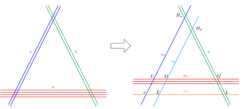
Figure 1: Pati-Salam gauge group ${\rm SU}(4)\times{\rm SU}(2)_{L}\times{\rm SU}(2)_{R}$ is broken down to the standard model gauge group ${\rm SU}(3)_{C}\times{\rm U}(2)_{L}\times{\rm U}(1)_{I3R}\times{\rm U}(1)_{B-L}$ via the process of brane splitting that corresponds to assigning VEVs to the adjoint scalars, which arise as open-string moduli associated with the positions of stacks $a$ and $c$ in the internal space.

Pati-Salam gauge group ${\rm SU}(4)\times{\rm SU}(2)_{L}\times{\rm SU}(2)_{R}$ is higgsed down to the standard model gauge group ${\rm SU}(3)_{C}\times{\rm U}(2)_{L}\times{\rm U}(1)_{I3R}\times{\rm U}(1)_{B-L}$ by assigning vacuum expectation values to the adjoint scalars which arise as open-string moduli associated to the stacks $a$ and $c$, see figure 1,

$${\color[rgb]{1,0,0}a} \rightarrow {\color[rgb]{1,0,0}a_{1}}+{\color[rgb]{1,.5,0}a_{2}},$$

$${\color[rgb]{0,0,1}c} \rightarrow {\color[rgb]{0,0,1}c_{1}}+{\color[rgb]{0,1,1}c_{2}}.$$ (12)

Moreover, the ${\rm U}(1)_{I_{3R}}\times{\rm U}(1)_{B-L}$ gauge symmetry may be broken to ${\rm U}(1)_{Y}$ by giving vacuum expectation values (VEVs) to the vector-like particles with the quantum numbers $({\bf{1},1,1/2,-1})$ and $({\bf{1},1,-1/2,1})$ under the ${\rm SU}(3)_{C}\times{\rm SU}(2)_{L}\times{\rm U}(1)_{I_{3R}}\times{\rm U}(1)_{B-L}$ gauge symmetry from $a_{2}c_{1}^{\prime}$ intersections Cvetic:2004ui ; Chen:2006gd .

This brane-splitting results in standard model quarks and leptons as Cvetic:2004nk ,

$$F_{L}(Q_{L},L_{L}) \rightarrow Q_{L}+L,$$

$$F_{R}(Q_{R},L_{R}) \rightarrow U_{R}+D_{R}+E_{R}+N.$$ (13)

Three-point Yukawa couplings for the quarks and the charged leptons can be read from the following superpotential,

$$W_{Y}=Y^{U}_{ijk}Q_{L}^{i}U_{R}^{j}H_{U}^{k}+Y^{D}_{ijk}Q_{L}^{i}D_{R}^{j}H_{D}^{k}+Y^{L}_{ijk}L^{i}E^{j}H_{D}^{k}.$$ (14)

The additional exotic particles must be made superheavy to ensure gauge coupling unification at the GUT scale. Similar to Refs. Cvetic:2007ku ; Chen:2007zu we can decouple the additional exotic particles except the four chiral multiplets under ${\rm SU}(4)_{C}$ anti-symmetric representation. And these four chiral multiplets can be decoupled via instanton effects in principle Blumenhagen:2006xt ; Haack:2006cy ; Florea:2006si , and we will present the detailed discussions elsewhere.

We now turn our attention toward the four dimensional low energy effective field theory. $\mathcal{N}=1$ supergravity action is encoded by three functions viz. the gauge kinetic function $f_{x}$, the Kähler potential $K$ and the superpotential $W$ Cremmer:1982en . Each of these functions in turn depend on dilaton $S$, complex $T$, and Kähler $U$ moduli.

The complex structure moduli $U$ can be obtained from the supersymmetry conditions as,

$$U^{i} =\frac{iR_{2}^{i}}{R_{1}^{i}+\frac{\beta_{i}}{2}iR_{2}^{i}}=\frac{i\chi^{i}}{1+\frac{\beta_{i}}{2}i\chi^{i}},\qquad\because\chi^{i}\equiv\frac{R_{2}^{i}}{R_{1}^{i}}.$$ (15)

These upper case moduli in string theory basis can be transformed in to lower case $s$, $t$, $u$ moduli in field theory basis as Lust:2004cx ,

$$\mathrm{Re}\,(s) =\frac{e^{-{\phi}_{4}}}{2\pi}\,\left(\frac{\sqrt{\mathrm{Im}\,U^{1}\,\mathrm{Im}\,U^{2}\,\mathrm{Im}\,U^{3}}}{|U^{1}U^{2}U^{3}|}\right),$$

$$\mathrm{Re}\,(u^{j}) =\frac{e^{-{\phi}_{4}}}{2\pi}\left(\sqrt{\frac{\mathrm{Im}\,U^{j}}{\mathrm{Im}\,U^{k}\,\mathrm{Im}\,U^{l}}}\right)\;\left|\frac{U^{k}\,U^{l}}{U^{j}}\right|,\quad(j,k,l)=(\overline{1,2,3}),$$

$$\mathrm{Re}(t^{j}) =\frac{i\alpha^{\prime}}{T^{j}},$$ (16)

where $j$ denotes the $j^{\rm th}$ two-torus, and $\phi_{4}$ is the four dimensional dilaton which is related to the supergravity moduli as

$$2\pi e^{\phi_{4}}=\Big{(}\mathrm{Re}(s)\,\mathrm{Re}(u_{1})\,\mathrm{Re}(u_{2})\,\mathrm{Re}(u_{3})\Big{)}^{-1/4}.$$ (17)

Inverting the above formulas we can solve for $U$ moduli in string theory basis in terms of $s$ and $u$ as,

$$\frac{|U^{j}|^{2}}{\mathrm{Im}\,(U^{j})}=\sqrt{\frac{\mathrm{Re}\,(u^{k})\,\mathrm{Re}\,(u^{l})}{\mathrm{Re}\,(u^{j})\mathrm{Re}\,(s)}},\quad(j,k,l)=(\overline{1,2,3}).$$ (18)

The holomorphic gauge kinetic function for any D6-brane stack $x$ wrapping a calibrated 3-cycle is given as Blumenhagen:2006ci ,

$$f_{x}=\frac{1}{2\pi\ell_{s}^{3}}\left[e^{-\phi}\int_{\Pi_{x}}\mbox{Re}(e^{-i\theta_{x}}\Omega_{3})-i\int_{\Pi_{x}}C_{3}\right],$$ (19)

where the integral involving 3-form $\Omega_{3}$ gives,

$$\int_{\Pi_{x}}\Omega_{3}=\frac{1}{4}\prod_{i=1}^{3}(n_{x}^{i}R_{1}^{i}+2^{-\beta_{i}}il_{x}^{i}R_{2}^{i}).$$ (20)

It can then be shown that,

$$f_{x} = \frac{1}{4\kappa_{x}}(n_{x}^{1}\,n_{x}^{2}\,n_{x}^{3}\,s-\frac{n_{x}^{1}\,l_{x}^{2}\,l_{x}^{3}\,u^{1}}{2^{(\beta_{2}+\beta_{3})}}-\frac{l_{x}^{1}\,n_{x}^{2}\,l_{x}^{3}\,u^{2}}{2^{(\beta_{1}+\beta_{3})}}-\frac{l_{x}^{1}\,l_{x}^{2}\,n_{x}^{3}\,u^{3}}{2^{(\beta_{1}+\beta_{2})}}),$$ (21)

where the factor ${\kappa}_{x}$ is related to the difference between the gauge couplings for ${\rm U}(N_{x})$ and $Sp(2N_{x}),\,SO(2N_{x})$. ${\kappa}_{x}=1$ for ${\rm U}(N_{x})$ and ${\kappa}_{x}=2$ for $Sp(2N_{x})$ or $SO(2N_{x})$ Klebanov:2003my . Since, the standard model hypercharge ${\rm U}(1)_{Y}$ is a linear combination of several ${\rm U}(1)$s,

$$Q_{Y}=\frac{1}{6}Q_{a_{1}}+\frac{1}{2}Q_{a_{2}}-\frac{1}{2}Q_{c_{1}}-\frac{1}{2}Q_{c_{2}}.$$ (22)

Therefore, the holomorphic gauge kinetic function for the hypercharge is also taken as a linear combination of the kinetic gauge functions from all of the stacks as Blumenhagen:2003jy ; Ibanez:2001nd ,

$$f_{Y}=\frac{1}{6}f_{a_{1}}+\frac{1}{2}f_{a_{2}}+\frac{1}{2}f_{c_{1}}+\frac{1}{2}f_{c_{2}}.$$ (23)

The Kähler potential to the second order for the moduli $M$ and open string matter fields $C_{i},C_{\theta}$ is given by :

$$K(M,\bar{M},C,\bar{C}) =\hat{K}(M,\bar{M})+\sum_{\mathrm{untwisted}\,i,j}\tilde{K}_{C_{i}\bar{C}_{j}}(M,\bar{M})C_{i}\bar{C}_{j}$$

$$\quad+\sum_{\mathrm{twisted},\,\theta}\tilde{K}_{C_{\theta}\bar{C}_{\theta}}(M,\bar{M})C_{\theta}\bar{C}_{\theta},$$ (24)

where $C_{i}$ correspond to the D-brane positions and the Wilson lines moduli arising from strings having both ends on the same stack while $C_{\theta}$ correspond to strings stretching between different stacks comprising $1/4$ BPS branes. The untwisted moduli fields $C_{i},\bar{C}_{j}$ are not present in MSSM and must become heavy via higher dimensional operators.

Let us determine the Kähler metric $\tilde{K}_{C_{\theta}\bar{C}_{\theta}}(M,\bar{M})$ for the twisted moduli. We denote the Kähler potential arising from strings stretching between stacks $x$ and $y$ as $\tilde{K}_{xy}$ and $\theta^{j}_{xy}\equiv\theta^{j}_{y}-\theta^{j}_{x}$ denotes the angle between the cycles wrapped by the branes $x$ and $y$ on the $j^{\rm th}$ two-torus with the constraint $\sum_{j}\theta^{j}_{xy}=0$. Following Font:2004cx ; Cvetic:2003ch ; Lust:2004cx , we find two cases for the Kähler metric in type IIA theory:

• $\theta^{j}_{xy}<0$, $\theta^{k}_{xy}>0$, $\theta^{l}_{xy}>0$

  $$\tilde{K}_{xy} = e^{\phi_{4}}e^{\gamma_{E}(2-\sum_{j=1}^{3}\theta^{j}_{xy})}\sqrt{\frac{\Gamma(\theta^{j}_{xy})}{\Gamma(1+\theta^{j}_{xy})}}\sqrt{\frac{\Gamma(1-\theta^{k}_{xy})}{\Gamma(\theta^{k}_{xy})}}\sqrt{\frac{\Gamma(1-\theta^{l}_{xy})}{\Gamma(\theta^{l}_{xy})}}$$ (25)

  $$(t^{j}+\bar{t}^{j})^{\theta^{j}_{xy}}(t^{k}+\bar{t}^{k})^{-1+\theta^{k}_{xy}}(t^{l}+\bar{t}^{l})^{-1+\theta^{l}_{xy}}.$$

• $\theta^{j}_{xy}<0$, $\theta^{k}_{xy}<0$, $\theta^{l}_{xy}>0$

  $$\tilde{K}_{xy} = e^{\phi_{4}}e^{\gamma_{E}(2+\sum_{j=1}^{3}\theta^{j}_{xy})}\sqrt{\frac{\Gamma(1+\theta^{j}_{xy})}{\Gamma(-\theta^{j}_{xy})}}\sqrt{\frac{\Gamma(1+\theta^{k}_{xy})}{\Gamma(-\theta^{k}_{xy})}}\sqrt{\frac{\Gamma(\theta^{l}_{xy})}{\Gamma(1-\theta^{l}_{xy})}}$$ (26)

  $$(t^{j}+\bar{t}^{j})^{-1-\theta^{j}_{xy}}(t^{k}+\bar{t}^{k})^{-1-\theta^{k}_{xy}}(t^{l}+\bar{t}^{l})^{-\theta^{l}_{xy}}.$$

The Kähler metric for the branes parallel to at least one torus which give rise to non-chiral matter in bifundamental representations (1/2 BPS scalar) like the Higgs doublet is,

$$\hat{K}_{\mathrm{higgs}}=\left[(s+\bar{s})(t^{1}+\bar{t}^{1})(t^{2}+\bar{t}^{2})(u^{3}+\bar{u}^{3})\right]^{-1/2}.$$ (27)

The superpotential is given as,

$$W=\hat{W}+\frac{1}{2}{\mu}_{\alpha\beta}(M)\,C^{\alpha}\,C^{\beta}+\frac{1}{6}\,Y_{\alpha\beta\gamma}(M)\,C^{\alpha}\,C^{\beta}\,C^{\gamma}+...$$ (28)

and the minimum of the tree-level F-term supergravity scalar potential is given by

$$V(M,\bar{M}) =e^{G}(G_{M}K^{MN}G_{N}-3)$$

$$=(F^{M}K_{MN}F^{N}-3e^{G}),$$ (29)

where $G_{M}=\partial_{M}G$, $K_{MN}=\partial_{M}\partial_{N}K$, $K^{MN}$ is the inverse Kähler metric, and the auxiliary fields $F^{M}$ are,

$$F^{M}=e^{G/2}K^{MN}G_{N}.$$ (30)

Thus supersymmetry is broken via F-terms from some of the hidden sector fields $M$ acquiring VEVs, thereby generating soft terms in the observable sector Font:2004cx ; Kane:2004hm ; Chen:2007zu . Gravitino gets massive by absorbing Goldstino via the superhiggs mechanism.

$$m_{3/2}=e^{G/2}.$$ (31)

The normalized soft parameters viz. the gaugino mass, squared scalar mass and trilinear parameters are given by Brignole:1997dp ,

$$M_{x} =\frac{1}{2\,\mathrm{Re}\,f_{x}}\,(F^{M}\,\partial_{M}\,f_{x}),$$

$$m_{xy}^{2} =(m_{3/2}^{2}+V_{0})-\sum_{M,N}\,\bar{F}^{\bar{M}}F^{N}\,{\partial}_{\bar{M}}\,{\partial}_{N}\,\log({\tilde{K}}_{xy}),$$

$$A_{xyz} =F^{M}[\hat{K}_{M}+{\partial}_{M}\,\log(Y_{xyz})-{\partial}_{M}\,\log(\tilde{K}_{xy}\tilde{K}_{yz}\tilde{K}_{zx})],$$ (32)

where $\hat{K}_{M}$ is the Kähler metric for branes parallel to at least one torus and $F^{M}$ denotes auxiliary fields.

Although it appears that soft terms may depend on the Yukawa couplings via the superpotential, however these are not the physical Yukawa couplings which exponentially depend on the worldsheet area as discussed in section 4. Both are related by the following relation,

$$Y^{\mathrm{phys}}_{xyz}=Y_{xyz}\,\frac{\hat{W}^{*}}{|\hat{W}|}\,e^{\hat{K}/2}\,(\tilde{K}_{x}\tilde{K}_{y}\tilde{K}_{z})^{-1/2}.$$ (33)

To calculate the soft terms from supersymmetry breaking we ignore the cosmological constant $V_{0}$ and introduce the following VEVs for the auxiliary fields (30) for the $s$, $t$ and $u$ moduli Brignole:1993dj ,

$$F^{s} =2\sqrt{3}Cm_{3/2}\mathrm{Re}(s)\Theta_{s}e^{-i\gamma_{s}},$$

$$F^{\{u,t\}^{i}} =2\sqrt{3}Cm_{3/2}\left(\mathrm{Re}({u}^{i})\Theta_{i}^{u}e^{-i\gamma^{u}_{i}}+\mathrm{Re}({t}^{i})\Theta_{i}^{t}e^{-i\gamma_{i}^{t}}\right),$$ (34)

Here, the factors $\gamma_{s}$ and $\gamma_{i}$ denote the CP violating phases of the moduli. The constant $C$ is given by the gravitino-mass $m^{2}_{3/2}$ and the cosmological constant $V_{0}$ as $C^{2}=1+\frac{V_{0}}{3m^{2}_{3/2}}$. $\Theta_{s}$ and $\Theta^{t,u}_{i}$ are the goldstino angles which determine the degree to which supersymmetry breaking is being dominated by any of the dilaton $s$, complex structure ($u^{i}$) and Kähler ($t^{i}$) moduli constrained by the relation,

$$\sum_{i=1}^{3}(|\Theta_{i}^{u}|^{2}+|\Theta_{i}^{t}|^{2})+|\Theta_{s}|^{2}=1.$$ (35)

Unlike the $s$- or $u$-moduli dominant supersymmetry breaking, the case of $t$-moduli dominant susy breaking depends on the physical Yukawa couplings via the area of the triangles and thus we shall only concentrate on the following two scenarios:

1. The $u$-moduli dominated supersymmetry breaking with the goldstino angle $\Theta_{s}$ set to zero, such that $F^{s}=F^{t^{i}}=0$.

2. The $u$ and $s$-moduli supersymmetry breaking with $F^{s}\neq 0$ .

The cosmological constant, $V_{0}$ is taken to be zero in all cases.

3.1 Supersymmetry breaking with $u$-moduli dominance

In the $u$-moduli dominant susy breaking $\Theta_{s}=0$ and the auxiliary fields (3) become,

$$F^{u^{i}}=\sqrt{3}m_{3/2}(u^{i}+\bar{u}^{i})\Theta_{i}e^{-i\gamma_{i}},\quad i=1,2,3.$$ (36)

To calculate the soft terms, we need to know the derivatives of the Kähler potential with respect to $u$. Defining $\tilde{K}_{xy}\equiv e^{{\phi}_{4}}\,\tilde{K}^{0}_{xy}$ and using (25) and (26), we compute the derivatives with respect to $u^{i}$ as,

$$\frac{\partial\log{\tilde{K}_{xy}}}{\partial u^{i}} = \sum_{j=1}^{3}\frac{\partial\log{\tilde{K}^{0}_{xy}}}{\partial\theta^{j}_{xy}}\frac{\partial\theta^{j}_{xy}}{\partial u^{i}}-\frac{1}{4(u^{i}+\bar{u}^{i})},$$ (37)

$$\frac{\partial^{2}\log{\tilde{K}_{xy}}}{\partial u^{i}\partial\bar{,}u^{j}} = \sum_{k=1}^{3}\left(\frac{\partial\log{\tilde{K}^{0}_{xy}}}{\partial\theta^{k}_{xy}}\frac{\partial^{2}\theta^{k}_{xy}}{\partial u^{i}\partial\bar{u}^{j}}+\frac{\partial^{2}\log\tilde{K}^{0}_{xy}}{\partial(\theta^{k}_{xy})^{2}}\frac{\partial\theta^{k}_{xy}}{\partial u^{i}}\frac{\partial\theta^{k}_{xy}}{\partial\bar{u}^{j}}+\frac{{\delta}_{ij}}{4\,(u^{i}+\bar{u}^{i})^{2}}\right).$$

From the Kähler potential in (26), we have

$$\Psi(\theta^{j}_{xy}) \equiv\frac{\partial\log{\tilde{K}^{0}_{xy}}}{\partial\theta^{j}_{xy}}=\gamma_{E}\!+\!\frac{1}{2}\frac{d}{d{\theta}^{j}_{xy}}\log{\Gamma(1-\theta^{j}_{xy})}-\frac{1}{2}\frac{d}{d{\theta}^{j}_{xy}}\log{\Gamma(\theta^{j}_{xy})}-\log(t^{j}+\bar{t}^{j}),$$ (38)

$$\Psi^{\prime}(\theta^{j}_{xy}) \equiv\frac{\partial^{2}\log\tilde{K}^{0}_{xy}}{\partial(\theta^{j}_{xy})^{2}}=\frac{d\Psi(\theta^{j}_{xy})}{d\theta^{j}_{xy}}.$$ (39)

The angles $\theta^{j}_{xy}\equiv\theta^{j}_{y}-\theta^{j}_{x}$ are related to the $u$ moduli as,

$$\tan(\pi\theta^{j}_{x})=\frac{2^{-\beta_{j}}l^{j}_{x}}{n^{j}_{x}}\sqrt{\frac{\mathrm{Re}u^{k}\,\mathrm{Re}u^{l}}{\mathrm{Re}u^{j}\,\mathrm{Re}s}}\quad\mathrm{where~{}}(j,k,l)=(\overline{1,2,3}).$$ (40)

And the derivative of the angles are defined as,

$${\theta}^{j,k}_{xy}\equiv(u^{k}+\bar{u}^{k})\,\frac{\partial\theta^{j}_{xy}}{\partial u^{k}}=\left\{\begin{array}[]{l}\left[-\frac{1}{4\pi}\sin(2\pi\theta^{j})\right]^{x}_{y}\quad\mathrm{when~{}}j=k\\ \left[\frac{1}{4\pi}\sin(2\pi\theta^{j})\right]^{x}_{y}\quad\mathrm{when~{}}j\neq k\end{array}\right.$$ (41)

where $[f(\theta^{j})]^{x}_{y}=f(\theta^{j}_{x})-f(\theta^{j}_{y})$. And the second order derivatives become,

$${\theta}^{j,k\bar{l}}_{xy}\equiv(u^{k}+\bar{u}^{k})(u^{l}+\bar{u}^{l})\,\frac{\partial^{2}\theta^{j}_{xy}}{\partial u^{k}\partial\bar{u}^{l}}=\left\{\begin{array}[]{l}\frac{1}{16\pi}\left[\sin(4\pi\theta^{j})+4\sin(2\pi\theta^{j})\right]^{x}_{y}\quad\mathrm{when~{}}j=k=l\\ \frac{1}{16\pi}\left[\sin(4\pi\theta^{j})-4\sin(2\pi\theta^{j})\right]^{x}_{y}\quad\mathrm{when~{}}j\neq k=l\\ -\frac{1}{16\pi}\left[\sin(4\pi\theta^{j})\right]^{x}_{y}\quad\mathrm{when~{}}j=k\neq l\mathrm{~{}or~{}}j=l\neq k\\ \frac{1}{16\pi}\left[\sin(4\pi\theta^{j})\right]^{x}_{y}\quad\mathrm{when~{}}j\neq k\neq l\neq j\end{array}\right.$$ (42)

We can now substitute the parametrizations (36)-(39) in the general expressions (32) to calculate the soft terms:

• Gaugino mass parameters:

  $$M_{x}=\frac{-\sqrt{3}m_{3/2}}{4\mathrm{Re}f_{x}}\sum_{j=1}^{3}\left(\mathrm{Re}u^{j}\,\Theta_{j}\,e^{-i\gamma_{j}}\,2^{-(\beta_{k}+\beta_{l})}n^{j}_{x}l^{k}_{x}l^{l}_{x}\right),$$

  $$(j,k,l)=(\overline{1,2,3}).$$ (43)

  Bino mass parameter is then related to the linear combination of the gaugino masses for each stack as,

  $$M_{Y}=\frac{1}{f_{Y}}\sum_{x}c_{x}f_{x}M_{x},$$ (44)

  where the coefficients $c_{x}$ correspond to the linear combination of ${\rm U}(1)$ factors which define the hypercharge, ${\rm U}(1)_{Y}=\sum c_{x}{\rm U}(1)_{x}$, cf. (23).

• Trilinear parameters:

  $$A_{xyz} =-\sqrt{3}m_{3/2}\sum_{j=1}^{3}\left[\Theta_{j}e^{-i\gamma_{j}}\left(\frac{1}{2}+\sum_{k=1}^{3}\theta_{xy}^{k,j}\Psi(\theta^{k}_{xy})+\sum_{k=1}^{3}\theta_{zx}^{k,j}\Psi(\theta^{k}_{zx})\right)\right]$$

  $$\quad+\frac{\sqrt{3}}{2}m_{3/2}{\Theta}_{3}e^{-i{\gamma}_{1}},$$ (45)

  where $x$, $y$, and $z$ label those stacks of branes whose intersections define the corresponding fields present in the trilinear coupling. Since the differences of the angles may be negative $\theta_{xy}=\theta_{y}-\theta_{x}$, it is useful to define the sign parameter,

  $$\eta_{xy}=\prod_{i}(-1)^{1-H(\theta_{xy}^{i})},\quad H(x)=\begin{cases}0,&x<0\\ 1,&x\geq 0\end{cases}$$ (46)

  where the value $\eta_{xy}=-1$ indicates that only one of the angle differences is negative while $\eta_{xy}=+1$ indicates that two of the angle differences are negative.

• Squarks and sleptons mass-squared (1/4 BPS scalars):

  $$m^{2}_{xy}=m_{3/2}^{2}\left[1-3\sum_{m,n=1}^{3}\Theta_{m}\Theta_{n}e^{-i(\gamma_{m}-\gamma_{n})}\left(\frac{{\delta}_{mn}}{4}+\sum_{j=1}^{3}\left(\theta^{j,m\bar{n}}_{xy}\Psi(\theta^{j}_{xy})+\theta^{j,m}_{xy}\theta^{j,\bar{n}}_{xy}\Psi^{\prime}(\theta^{j}_{xy})\right)\right)\right].$$

  Here, the functions $\Psi(\theta_{xy})=\frac{\partial\log(e^{-\phi_{4}}\tilde{K}_{xy})}{\partial\theta_{xy}}$ in the case of $\eta_{xy}=-1$ are

  $$\mathrm{if}\ \theta_{xy}<0 :$$ (48)

  $$\Psi(\theta^{j}_{xy}) = -\gamma_{E}+\frac{1}{2}\frac{d}{d{\theta}^{j}_{xy}}\,\log{\Gamma(-\theta^{j}_{xy})}-\frac{1}{2}\frac{d}{d{\theta}^{j}_{xy}}\,\log{\Gamma(1+\theta^{j}_{xy})}+\log(t^{j}+\bar{t}^{j})$$

  $$\mathrm{if}\ \theta_{xy}>0 :$$

  $$\Psi(\theta^{j}_{xy}) = -\gamma_{E}+\frac{1}{2}\frac{d}{d{\theta}^{j}_{xy}}\,\log{\Gamma(1-\theta^{j}_{xy})}-\frac{1}{2}\frac{d}{d{\theta}^{j}_{xy}}\,\log{\Gamma(\theta^{j}_{xy})}+\log(t^{j}+\bar{t}^{j}),$$

  and in the case of $\eta_{xy}=+1$ are

  $$\mathrm{if}\ \theta_{xy}<0 :$$ (49)

  $$\Psi(\theta^{j}_{xy}) = \gamma_{E}+\frac{1}{2}\frac{d}{d{\theta}^{j}_{xy}}\,\log{\Gamma(1+\theta^{j}_{xy})}-\frac{1}{2}\frac{d}{d{\theta}^{j}_{xy}}\,\log{\Gamma(-\theta^{j}_{xy})}-\log(t^{j}+\bar{t}^{j})$$

  $$\mathrm{if}\ \theta_{xy}>0 :$$

  $$\Psi(\theta^{j}_{xy}) = \gamma_{E}+\frac{1}{2}\frac{d}{d{\theta}^{j}_{xy}}\,\log{\Gamma(\theta^{j}_{xy})}-\frac{1}{2}\frac{d}{d{\theta}^{j}_{xy}}\,\log{\Gamma(1-\theta^{j}_{xy})}-\log(t^{j}+\bar{t}^{j}),$$

  and $\Psi^{\prime}(\theta_{xy})$ is just the derivative $\Psi^{\prime}(\theta^{j}_{xy})=\frac{d\Psi(\theta^{j}_{xy})}{d\theta^{j}_{xy}}$.

• Higgs (1/2 BPS scalar) mass-squared is computed using the Kähler metric (27) as:

  $$m^{2}_{H}=m^{2}_{3/2}\left(1-\frac{3}{2}\left|\Theta_{3}\right|^{2}\right).$$ (50)

3.2 Supersymmetry breaking via $u$-moduli and dilaton $s$

Now we also include a non-zero VEV for the dilaton $s$ in the auxiliary fields (3) to get,

$$F^{s,u^{i}}=\sqrt{3}m_{3/2}[(s+\bar{s})\Theta_{s}e^{-i\gamma_{s}}+(u^{i}+\bar{u}^{i})\Theta_{i}e^{-i\gamma_{i}}].$$ (51)

Substituting above parametrization (51) and the expressions (36)-(39) in the general formulas (32), the soft parameters are found as follows:

• Gaugino mass parameters:

  $$M_{x}=\frac{-\sqrt{3}m_{3/2}}{4\mathrm{Re}f_{x}}\Bigg{[}\sum_{j=1}^{3}\mathrm{Re}(u^{j})\,\Theta_{j}\,e^{-i\gamma_{j}}\,2^{-(\beta_{k}+\beta_{l})}n^{j}_{x}l^{k}_{x}l^{l}_{x}+\Theta_{s}\mathrm{Re}(s)e^{-i\gamma_{0}}n_{x}^{1}\,n_{x}^{2}\,n_{x}^{3}\,\Bigg{]},$$

  $$(j,k,l)=(\overline{1,2,3}).\qquad\qquad\qquad$$ (52)

  and the Bino mass parameter is similarly defined as (44).

• Trilinear parameters:

  $$A_{xyz} =-\sqrt{3}m_{3/2}\sum_{j=1}^{4}\left[\Theta_{j}e^{-i\gamma_{j}}\left(\frac{1}{2}+\sum_{k=1}^{3}\theta_{xy}^{k,j}\Psi(\theta^{k}_{xy})+\sum_{k=1}^{3}\theta_{zx}^{k,j}\Psi(\theta^{k}_{zx})\right)\right]$$

  $$\quad+\frac{\sqrt{3}}{2}m_{3/2}\left({\Theta}_{3}e^{-i{\gamma}_{3}}+\Theta_{s}e^{-i{\gamma}_{s}}\right),$$ (53)

  where $j=4$ corresponds to $\Theta_{s}$.

• Squarks and sleptons mass-squared (1/4 BPS scalars):

  $$m^{2}_{xy} =m_{3/2}^{2}\left[1-3\sum_{m,n=1}^{4}\Theta_{m}\Theta_{n}e^{-i(\gamma_{m}-\gamma_{n})}\left(\frac{{\delta}_{mn}}{4}+\sum_{j=1}^{3}\left(\theta^{j,m\bar{n}}_{xy}\Psi(\theta^{j}_{xy})+\theta^{j,m}_{xy}\theta^{j,\bar{n}}_{xy}\Psi^{\prime}(\theta^{j}_{xy})\right)\right)\right],$$

  where now $\Theta_{4}\equiv\Theta_{s}$ is also included in the sum while the functions $\Psi(\theta_{xy})$, $\Psi^{\prime}(\theta_{xy})$ and the terms ${\theta}^{j,k}_{xy}$, ${\theta}^{j,k\bar{l}}_{xy}$ are defined similarly as before in equations (38), (39), (41) and (42). While the terms associated with the dilaton $s$ are given as,

  $${\theta}^{j,s}_{xy}\equiv(s+\bar{s})\,\frac{\partial\theta^{j}_{xy}}{\partial s}=-\frac{1}{4\pi}\left[\sin(2\pi\theta^{j})\right]^{x}_{y},$$ (55)

  $${\theta}^{j,k\bar{s}}_{xy}\equiv(u^{k}+\bar{u}^{k})(s+\bar{s})\,\frac{\partial^{2}\theta^{j}_{xy}}{\partial u^{k}\partial\bar{s}}=\left\{\begin{array}[]{l}\frac{1}{16\pi}\left[\sin{4\pi\theta^{j}}\right]^{x}_{y}\quad\mathrm{when}\ j=k\\ -\frac{1}{16\pi}\left[\sin{4\pi\theta^{j}}\right]^{x}_{y}\quad\mathrm{when}\ j\neq k,\end{array}\right.$$ (56)

  and

  $${\theta}^{j,s\bar{s}}_{xy}\equiv(s+\bar{s})(s+\bar{s})\,\frac{\partial^{2}\theta^{j}_{xy}}{\partial s\partial\bar{s}}=\frac{1}{16\pi}\left[\sin{4\pi\theta^{j}}+4\sin(2\pi\theta^{j})\right]^{x}_{y},$$ (57)

  where $k,l\neq s$.

• Higgs mass-squared (1/2 BPS scalar):

  $$m^{2}_{H}=m^{2}_{3/2}\left[1-\frac{3}{2}\left(\left|\Theta_{3}\right|^{2}+\left|\Theta_{s}\right|^{2}\right)\right].$$ (58)

3.3 Soft terms from susy breaking

We now systematically compute the soft terms from susy breaking in the general case of $u$-moduli dominance with dilaton modulus $s$ turned on. The complex structure moduli $U$ from (15) are,

$$\{U_{1},U_{2},U_{3}\} =\left\{\frac{i}{\sqrt{5}},\frac{7i}{\sqrt{5}},\frac{2}{9}\left(5+2i\sqrt{5}\right)\right\},$$ (59)

and the corresponding $u$-moduli and $s$-modulus in supergravity basis from (16) are,

$$\{u_{1},u_{2},u_{3}\} =\left\{\frac{\sqrt[4]{5}\sqrt{7}e^{-\phi_{4}}}{2\pi},\frac{\sqrt[4]{5}e^{-\phi_{4}}}{2\sqrt{7}\pi},\frac{\sqrt{7}e^{-\phi_{4}}}{2\ 5^{3/4}\pi}\right\},$$

$$s =\frac{\sqrt[4]{5}e^{-\phi_{4}}}{2\sqrt{7}\pi}.$$ (60)

Using (21) and the values from the table 3, the gauge kinetic function becomes,

$$\{f_{a},f_{b},f_{c}\} =\left\{\frac{27e^{-\phi_{4}}}{8\ 5^{3/4}\sqrt{7}\pi},\frac{9\sqrt[4]{5}e^{-\phi_{4}}}{16\sqrt{7}\pi},\frac{9\sqrt{7}e^{-\phi_{4}}}{16\ 5^{3/4}\pi}\right\},$$ (61)

To calculate gaugino masses $M_{1,2,3}$ respectively for ${\rm U}(1)_{Y}$, ${\rm SU}(2)_{L}$ and ${\rm SU}(3)_{c}$ gauge groups, we first compute $M_{a,b,c}$ using (• ‣ 3.2) as,

$$M_{a} =\frac{m_{3/2}}{18\sqrt{3}}\Big{(}35\Theta_{1}e^{i\gamma_{1}}-5\Theta_{2}e^{-i\gamma_{2}}+14\Theta_{3}e^{-i\gamma_{3}}-10\Theta_{4}e^{-i\gamma_{4}}\Big{)},$$

$$M_{b} =\frac{m_{3/2}}{3\sqrt{3}}\left(5e^{-i\gamma_{2}}\Theta_{2}-4e^{-i\gamma_{4}}\Theta_{4}\right),$$

$$M_{c} =\frac{m_{3/2}}{3\sqrt{3}}\left(5e^{-i\gamma_{1}}\Theta_{1}+4e^{-i\gamma_{3}}\Theta_{3}\right).$$ (62)

Bino mass parameter $M_{Y}$ (44) is then computed as,

$$M_{Y} =\frac{m_{3/2}}{99\sqrt{3}}\left(175\Theta_{1}e^{-i\gamma_{1}}-10\Theta_{2}e^{-i\gamma_{2}}+112\Theta_{3}e^{-i\gamma_{3}}-20\Theta_{4}e^{-i\gamma_{4}}\right).$$ (63)

Therefore, the gaugino masses for ${\rm U}(1)_{Y}$, ${\rm SU}(2)_{L}$ and ${\rm SU}(3)_{c}$ gauge groups are,

$$M_{1} \equiv M_{Y}=\frac{m_{3/2}}{99\sqrt{3}}\left(175\Theta_{1}e^{-i\gamma_{1}}-10\Theta_{2}e^{-i\gamma_{2}}+112\Theta_{3}e^{-i\gamma_{3}}-20\Theta_{4}e^{-i\gamma_{4}}\right),$$

$$M_{2} \equiv M_{b}=\frac{m_{3/2}}{3\sqrt{3}}\left(5e^{-i\gamma_{2}}\Theta_{2}-4e^{-i\gamma_{4}}\Theta_{4}\right),$$

$$M_{3} \equiv M_{a}=\frac{m_{3/2}}{18\sqrt{3}}\Big{(}35\Theta_{1}e^{i\gamma_{1}}-5\Theta_{2}e^{-i\gamma_{2}}+14\Theta_{3}e^{-i\gamma_{3}}-10\Theta_{4}e^{-i\gamma_{4}}\Big{)}.$$ (64)

Table 5: The angles (in multiples of $\pi$) with respect to the orientifold plane made by the cycle wrapped by each stack of D-branes on each of the three two-tori.

	$\pi\theta^{1}$	$\pi\theta^{2}$	$\pi\theta^{3}$
$a$	$-\tan^{-1}\left(\frac{1}{\sqrt{5}}\right)$	$\tan^{-1}\left(\frac{7}{\sqrt{5}}\right)$	$-\tan^{-1}\left(\frac{\sqrt{5}}{2}\right)$
$b$	$-\tan^{-1}\left(\frac{\sqrt{5}}{2}\right)$	$0$	$\tan^{-1}\left(\frac{\sqrt{5}}{2}\right)$
$c$	$\tan^{-1}\left(\frac{2}{\sqrt{5}}\right)$	$-\frac{\pi}{2}$	$\tan^{-1}\left(\frac{\sqrt{5}}{2}\right)$

Next, to compute the trilinear coupling and the sleptons mass-squared we require the angles, the differences of angles and their first and second order derivatives with respect to the moduli. In table 5 we show the angles made by the cycle wrapped by each stack D6 branes with respect to the orientifold plane,

$$\pi\theta_{x}^{i} =\tan^{-1}\left(\frac{2^{-\beta_{i}}l_{x}^{i}\chi_{i}}{n_{x}^{i}}\right).$$ (65)

The differences of the angles, $\theta_{xy}^{i}\equiv\theta_{y}^{i}-\theta_{x}^{i}$ are,

$$\left(\begin{array}[]{ccc}\hskip-50.00008pt\{0.,0.,0.\}&\hskip-70.0001pt\{-0.13386,-0.401581,0.535441\}&\{0.36614,-0.901581,0.535441\}\\ \{0.13386,0.401581,-0.535441\}&\{0.,0.,0.\}&\{0.5,-0.5,0.\}\\ \{-0.36614,0.901581,-0.535441\}&\{-0.5,0.5,0.\}&\{0.,0.,0.\}\\ \end{array}\right)$$ (69)

To account for the negative angle differences it is convenient to define the sign function $\sigma_{xy}^{i}$, which is $-1$ only for negative angle difference and $+1$ otherwise,

$$\sigma_{xy}^{i}\equiv(-1)^{1-H(\theta_{xy}^{i})} =\left(\begin{array}[]{ccc}\{1,1,1\}&\{-1,-1,1\}&\{1,-1,1\}\\ \{1,1,-1\}&\{1,1,1\}&\{1,-1,1\}\\ \{-1,1,-1\}&\{-1,1,1\}&\{1,1,1\}\\ \end{array}\right),$$ (73)

where $H(x)$ is the unit step function. And the function $\eta_{xy}$ can thus be defined by taking the product on the torus index $i$ as,

$$\eta_{xy}\equiv\prod_{i}\sigma_{xy}^{i}=\left(\begin{array}[]{ccc}1&1&-1\\ -1&1&-1\\ 1&-1&1\\ \end{array}\right).$$ (74)

Using above defined $\sigma_{xy}^{i}$ and $\eta_{xy}^{i}$, we can readily write the four cases of functions $\Psi(\theta_{xy})$ defined in (48) and (49) into a single expression as,

$$\Psi(\theta^{j}_{xy}) =\eta_{xy}\left(\frac{1}{2}\psi^{(0)}(\sigma_{xy}^{i}\theta^{j}_{xy})+\frac{1}{2}\psi^{(0)}(1-\sigma_{xy}^{i}\theta^{j}_{xy})+\gamma_{E}-\log(t^{j}+\bar{t}^{j})\right),$$ (75)

where $\psi^{(0)}(z)$ is called the digamma function defined as the derivative of the logarithm of the gamma function. The successive derivatives of the $\log\Gamma(z)$ yield the polygamma function $\psi^{(n)}(z)$ as,

$$\psi^{(n-1)}(z)=\frac{d^{(n)}}{dz^{(n)}}\log\Gamma(z),$$ (76)

with the following properties,

$$\frac{d}{dz}\psi^{(0)}(\pm z) =\pm\psi^{(1)}(\pm z),$$

$$\frac{d}{dz}\psi^{(0)}(1\pm z) =\pm\psi^{(1)}(1\pm z).$$ (77)

Similarly, the derivative $\Psi^{\prime}(\theta^{j}_{xy})=\frac{d\Psi(\theta^{j}_{xy})}{d\theta^{j}_{xy}}$ can be expressed succinctly as,

$$\Psi^{\prime}(\theta^{j}_{xy}) =\eta_{xy}\sigma_{xy}^{i}\left(\frac{1}{2}\psi^{(1)}(\sigma_{xy}^{i}\theta^{j}_{xy})+\frac{1}{2}\psi^{(1)}(1-\sigma_{xy}^{i}\theta^{j}_{xy})\right),$$ (78)

where we have utilized the property (3.3) and have neglected the contribution of the $t$-moduli.

Lastly, by making use of appropriate Kronecker deltas and defining $u^{4}\equiv s$, we can express the various cases of the first and second derivatives of the angles as,

$${\theta}^{i,m}_{xy}\equiv(u^{m}+\bar{u}^{m})\,\frac{\partial\theta^{i}_{xy}}{\partial u^{m}}=(-1)^{\delta_{m,4}}(-1)^{\delta_{i,j}}\frac{\sin(2\pi\theta^{i})}{4\pi}\bigg{|}^{x}_{y},$$

$$i={1,2,3};\quad m={1,2,3,4.}$$ (79)

$${\theta}^{i,mn}_{xy} \equiv(u^{m}+\bar{u}^{m})(u^{n}+\bar{u}^{n})\,\frac{\partial^{2}\theta^{i}_{xy}}{\partial u^{m}\partial\bar{u}^{n}}$$

$$=\delta_{m,n}\frac{\sin(4\pi\theta^{i})+(-1)^{(1-\delta_{4,m})(1-\delta_{i,m})}4\sin(2\pi\theta^{i})}{16\pi}\bigg{|}^{x}_{y}$$

$$\quad+(1-\delta_{m,n})(-1)^{(1-\delta_{4,m})(1-\delta_{4,n})(\delta_{i,m}+\delta_{i,n})}(-1)^{1-\delta_{i,m}-\delta_{i,n}}\frac{\sin(4\pi\theta^{i})}{16\pi}\bigg{|}^{x}_{y}$$

$$\qquad\qquad\qquad\qquad\qquad\qquad\qquad\qquad\quad i={1,2,3};\quad m,n={1,2,3,4}.$$ (80)

Utilizing above results while ignoring the CP-violating phases $\gamma^{i}$, the gaugino masses, trilinear coupling (• ‣ 3.2) and sleptons and squarks mass-squared (• ‣ 3.2) parameters are obtained as follows,

$$M_{1} =m_{3/2}(1.02057\Theta_{1}-0.0583182\Theta_{2}+0.653164\Theta_{3}-0.116636\Theta_{4}),$$

$$M_{2} =m_{3/2}(0.96225\Theta_{2}-0.7698\Theta_{4}),$$

$$M_{3} =m_{3/2}(1.12263\Theta_{1}-0.160375\Theta_{2}+0.44905\Theta_{3}-0.32075\Theta_{4}),$$

$$A_{0} \equiv A_{abc}=A_{acb}=m_{3/2}\Big{(}-1.65515\Theta_{1}-0.0769026\Theta_{2}+0.210438\Theta_{3}-0.210438\Theta_{4}\Big{)},$$

$$m^{2}_{L} \equiv m^{2}_{ab}=m_{3/2}{}^{2}\Big{(}1-0.691918\Theta_{1}{}^{2}-0.251923\Theta_{1}\Theta_{2}+1.38697\Theta_{1}\Theta_{3}+0.297487\Theta_{1}\Theta_{4}$$

$$\quad\quad\quad-0.730464\Theta_{2}{}^{2}+1.38697\Theta_{2}\Theta_{3}+1.05521\Theta_{2}\Theta_{4}-2.46331\Theta_{3}{}^{2}$$

$$\quad\quad\quad-0.104624\Theta_{3}\Theta_{4}-1.61046\Theta_{4}{}^{2}\Big{)},$$

$$m^{2}_{R} \equiv m^{2}_{ac}=m_{3/2}{}^{2}\Big{(}1+0.672202\Theta_{1}{}^{2}+0.024956\Theta_{1}\Theta_{2}-2.83616\Theta_{1}\Theta_{3}+0.335005\Theta_{1}\Theta_{4}$$

$$\quad\quad\quad-2.02285\Theta_{2}{}^{2}-0.113933\Theta_{2}\Theta_{3}-1.68771\Theta_{2}\Theta_{4}+0.712303\Theta_{3}{}^{2}$$

$$\quad\quad\quad-0.122343\Theta_{3}\Theta_{4}+0.588437\Theta_{4}{}^{2}\Big{)}.$$ (81)

All above results are subject to the constraint,

$$\Theta_{1}^{2}+\Theta_{2}^{2}+\Theta_{3}^{2}+\Theta_{4}^{2}=1.$$ (82)

In Appendix A, we also compute the soft terms for the model with exact gauge coupling unification that was previously studied in ref. Chen:2007zu .

4 Yukawa couplings

Yukawa couplings arise from open string world-sheet instantons that connect three D-brane intersections Aldazabal:2000cn . Intersecting D6-branes at angles wrap 3-cycles on the compact space $\mathbf{T^{6}}=\mathbf{T^{2}}\times\mathbf{T^{2}}\times\mathbf{T^{2}}$. For instance in the case of three stacks of D-branes wrapping on a $\mathbf{T^{2}}$ the 3-cycles can be represented by the wrapping numbers in a vector form as:

$$[\Pi_{a}]=(n_{a},l_{a})\rightarrow z_{a}=R(n_{a}+\tau l_{a})\cdot x_{a},$$ (83)

$$[\Pi_{b}]=(n_{b},l_{b})\rightarrow z_{b}=R(n_{b}+\tau l_{b})\cdot x_{b},$$

$$[\Pi_{c}]=(n_{c},l_{c})\rightarrow z_{c}=R(n_{c}+\tau l_{c})\cdot x_{c},$$

where $\tau$ is the complex structure parameter, $(n_{a},l_{a})\in\mathbb{Z}^{2}$ is the wrapped 1-cycle, $x\in\mathbb{R}$ and $z_{a}\in\mathbb{C}$ respective to the brane $a$. The triangles bounded by the triplet of D-branes $(z_{a},z_{b},z_{c})$ will contribute to the Yukawa couplings Cremades:2003qj . A closer condition,

$$z_{a}+z_{b}+z_{c}=0,$$ (84)

ensures that triangles are actually formed by the three branes. The Diophantine equation (83) together with the closer condition can be solved to get the following solution:

$$x_{a}=\frac{I_{bc}}{d}x,$$

$$x_{b}=\frac{I_{ca}}{d}x,\quad x=x_{0}+l,$$

$$x_{c}=\frac{I_{ab}}{d}x,$$ (85)

where $I_{ab}$ is the intersection number, $d=g.c.d.(I_{ab},I_{bc},I_{ca})$ is the greatest common divisor of the intersection numbers, $l\in\mathbb{Z}$ arises from triangles connecting different points in the covering space $\mathbf{T^{6}}$ but the same points under the lattice $\mathbf{T^{2}}$ of the triangles and $x_{0}\in\mathbb{R}$ depends on the relative positions of the branes and the particular triplet $(i,j,k)$ of intersection points,

$$i=0,1,\cdots,|I_{ab}|-1,$$

$$j=0,1,\cdots,|I_{bc}|-1,$$

$$k=0,1,\cdots,|I_{ca}|-1,$$ (86)

such that $x_{0}$ can be written as

$$x_{0}(i,j,k)=\frac{i}{I_{ab}}+\frac{j}{I_{bc}}+\frac{k}{I_{ca}}.$$ (87)

Relaxing the condition that all branes intersect at the origin, we can introduce brane shifts $\epsilon_{\alpha}$, $\alpha=a,b,c$ to write a general expressions for $x_{0}$ as

$$x_{0}(i,j,k)=\frac{i}{I_{ab}}+\frac{j}{I_{bc}}+\frac{k}{I_{ca}}+\frac{d(I_{ab}\epsilon_{c}+I_{ca}\epsilon_{b}+I_{ab}\epsilon_{a})}{I_{ab}I_{bc}I_{ca}},$$ (88)

where we can absorb these three parameters into only one as,

$$\epsilon=\frac{I_{ab}\epsilon_{c}+I_{ca}\epsilon_{b}+I_{bc}\epsilon_{a}}{I_{ab}I_{bc}I_{ca}}.$$ (89)

This is obvious due to the reparametrization invariance in $\mathbf{T}^{2}$ since we can always choose two branes to intersect at the origin and the only remaining freedom left is the shift of third brane. The formula of the areas of the triangles can then be expressed using (88) as,

$$A(z_{a},z_{b})=\frac{1}{2}\sqrt{|z_{a}|^{2}|z_{b}|^{2}-(\mathrm{Re}z_{a}\bar{z}_{b})^{2}}$$

$$\rightarrow A_{ijk}(l)=\frac{1}{2}(2\pi)^{2}A|I_{ab}I_{bc}I_{ca}|(\frac{i}{I_{ab}}+\frac{j}{I_{bc}}+\frac{k}{I_{ca}}+\epsilon+l)^{2},$$ (90)

where $A$ is the Kähler structure of the torus. Finally, the Yukawa coupling for the three states localized at the intersections indexed by $(i,j,k)$ is given as,

$$Y_{ijk}=h_{qu}\sigma_{abc}\sum_{l\in Z}\exp(-\frac{A_{ijk}(l)}{2\pi\alpha^{\prime}}),$$ (91)

where the real phase $\sigma_{abc}={\rm sign}(I_{ab}I_{bc}I_{ca})$ comes from the full instanton contribution Cremades:2003qj and $h_{qu}$ is due to quantum correction as discussed in Cvetic:2003ch . For the ease of numerical computation real modular theta function is used to re-express the summation as

$$\vartheta\left[\begin{array}[]{c}\delta\\ \phi\end{array}\right](t)=\sum_{l\in\mathbf{Z}}e^{-\pi t(\delta+l)^{2}}e^{2l\pi i(\delta+l)\phi},$$ (92)

where the corresponding parameters are related as,

$$\delta=\frac{i}{I_{ab}}+\frac{j}{I_{bc}}+\frac{k}{I_{ca}}+\epsilon,$$

$$\phi=0,$$

$$t=\frac{A}{\alpha^{\prime}}|I_{ab}I_{bc}I_{ca}|.$$ (93)

Notice that the theta function $\vartheta$ is real, however $t$ can be complex while $\phi$ is an overall phase.

4.1 Adding a $B$-field and Wilson lines

Strings being one dimensional naturally couple to a 2-form $B$-field in addition to the metric. To incorporate the turning on of this $B$-field leads to a complex Kähler structure of the compact space $\mathbf{T^{2}}$ such that,

$$J=B+iA,$$ (94)

and the otherwise real parameter $t$ is changed to a complex parameter $\kappa$ as,

$$\kappa=\frac{J}{\alpha^{\prime}}|I_{ab}I_{bc}I_{ca}|.$$ (95)

Secondly, we can also add Wilson lines around the compact directions wrapped by the D-branes. However, to avoid breaking any gauge symmetry Wilson lines must be chosen corresponding to group elements in the centre of the gauge group, i.e., a phase Cremades:2003qj . For a triangle formed by three D-branes $a$, $b$ and $c$ each wrapping a different 1-cycle inside of $\mathbf{T}^{2}$, the Wilson lines can be given by the corresponding phases $\exp(2\pi i\theta_{a})$, $\exp(2\pi i\theta_{b})$, and $\exp(2\pi i\theta_{c})$ respectively. The total phase picked up by an open string sweeping such triangle will depend upon the relative longitude of each segment, determined by the intersection points:

$$e^{2\pi ix_{a}\theta_{a}}e^{2\pi ix_{b}\theta_{b}}e^{2\pi ix_{c}\theta_{c}}=e^{2\pi ix(I_{bc}\theta_{a}+I_{ca}\theta_{b}+I_{ab}\theta_{c})}.$$ (96)

In general, considering both a $B$-field as well as Wilson lines we get a complex theta function as

$$\vartheta\left[\begin{array}[]{c}\delta\\ \phi\end{array}\right](\kappa)=\sum_{l\in\mathbf{Z}}e^{\pi i\kappa(\delta+l)^{2}}e^{2\pi i(\delta+l)\phi},$$ (97)

where

$$\delta =\frac{i}{I_{ab}}+\frac{j}{I_{bc}}+\frac{k}{I_{ca}}+\epsilon,$$

$$\phi =I_{ab}\theta_{c}+I_{bc}\theta_{a}+I_{ca}\theta_{b},$$

$$\kappa =\frac{J}{\alpha^{\prime}}|I_{ab}I_{bc}I_{ca}|.$$ (98)

4.2 O-planes and non-prime intersection numbers

To cancel the RR-tadpoles we need to introduce the orientifold O-planes that are objects of negative tension. In addition for each D-brane $a$, we must include its mirror image $a^{\prime}$ under $\Omega R$. Such mirror branes will in general wrap a different cycle $\Pi_{a*}$, related to $\Pi_{a}$ by the action of $R$ on the homology of the torus. Consequently we also need to include the triangles formed by either of the branes or their images. As an example the Yukawa coupling from the branes $a$, $b^{\prime}$, and $c$ will depend on the parameters $I_{ab^{\prime}}$, $I_{b^{\prime}c}$, and $I_{ca}$, where the primed indexes are independent of the unprimed ones.

Furthermore, the three intersection numbers may not be coprime in general. Therefore, to avoid overcounting we need to involve the $g.c.d.$ of the intersection numbers as $d=g.c.d.(I_{ab},I_{bc},I_{ca})$.

Finally, to ensure that triangles are bounded by D-branes, the intersection indices must satisfy the following condition Cremades:2003qj

$$i+j+k=0\ {\rm~{}mod}\ d.$$ (99)

4.3 The general formula of Yukawa couplings

Therefore, the most general formula for Yukawa couplings for D6-branes wrapping a compact $\mathbf{T^{2}}\times\mathbf{T^{2}}\times\mathbf{T^{2}}$ space can be written as, compact space as

$$Y_{\{ijk\}}=h_{qu}\sigma_{abc}\prod_{r=1}^{3}\vartheta\left[\begin{array}[]{c}\delta^{(r)}\\ \phi^{(r)}\end{array}\right](\kappa^{(r)}),$$ (100)

where

$$\vartheta\left[\begin{array}[]{c}\delta^{(r)}\\ \phi^{(r)}\end{array}\right](\kappa^{(r)})=\sum_{l_{r}\in\mathbf{Z}}e^{\pi i(\delta^{(r)}+l_{r})^{2}\kappa^{(r)}}e^{2\pi i(\delta^{(r)}+l_{r})\phi^{(r)}},$$ (101)

with $r=1,2,3$ denoting the three 2-tori. And the input parameters are defined by

$$\delta^{(r)}=\frac{i^{(r)}}{I_{ab}^{(r)}}+\frac{j^{(r)}}{I_{ca}^{(r)}}+\frac{k^{(r)}}{I_{bc}^{(r)}}+\frac{d^{(r)}(I_{ab}^{(r)}\epsilon_{c}^{(r)}+I_{ca}^{(r)}\epsilon_{b}^{(r)}+I_{bc}^{(r)}\epsilon_{a}^{(r)})}{I_{ab}I_{bc}I_{ca}}+\frac{s^{(r)}}{d^{(r)}},$$

$$\phi^{(r)}=\frac{I_{bc}^{(r)}\theta_{a}^{(r)}+I_{ca}^{(r)}\theta_{b}^{(r)}+I_{ab}^{(r)}\theta_{c}^{(r)}}{d^{(r)}},$$

$$\kappa^{(r)}=\frac{J^{(r)}}{\alpha^{\prime}}\frac{|I_{ab}^{(r)}I_{bc}^{(r)}I_{ca}^{(r)}|}{(d^{(r)})^{2}}.$$ (102)

The theta function defined in (97) is in general complicated to evaluate numerically. However, for the special case without $B$-field, defining $J^{\prime}=-iJ=A$ and $\kappa^{\prime}=-i\kappa$ the $\vartheta$ function takes a more manageable form,

$$\vartheta\left[\begin{array}[]{c}\delta\\ \phi\end{array}\right](\kappa^{\prime})=\sum_{l\in\mathbf{Z}}e^{-\pi\kappa^{\prime}(\delta+l)^{2}}e^{2\pi i(\delta+l)\phi},$$ (105)

$$\stackrel{{\scriptstyle\textrm{redefine}}}{{\longrightarrow}} \vartheta\left[\begin{array}[]{c}\delta\\ \phi\end{array}\right](\kappa)=e^{-\pi\kappa\delta^{2}}e^{2\pi i\delta\phi}\vartheta_{3}(\pi(\phi+i\kappa\delta),e^{-\pi\kappa}),$$ (108)

in terms of $\vartheta_{3}$, the Jacobi theta function of the third kind.

5 Semi-realistic Yukawa textures

Yukawa matrices for the Model 16 depicted in table 3 are of rank 3 and the three intersections required to form the disk diagrams for the Yukawa couplings all occur on the first torus as shown in figure 2. The second and third tori only contribute an overall constant that has no effect in computing the fermion mass ratios. Thus, it is sufficient for our purpose to only focus on the first torus to nearly reproduce the correct the masses of the standard model fermions.

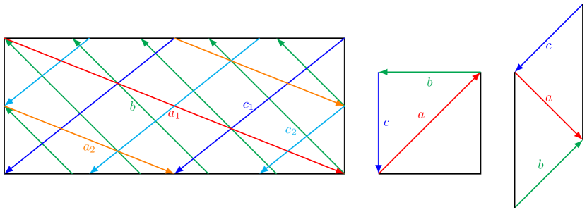
Figure 2: Brane configuration for the three 2-tori where the third 2-torus is tilted. Fermion mass hierarchies result from the intersections on the first 2-torus.

5.1 Mass matrices from 3-point functions

For the wrapping numbers listed in table 3, the intersection numbers on each torus are given as,

$$I_{ab}^{(1)}=3$$, , ,

, , ,

, , .

(109)

As the intersection numbers are not coprime, we define the greatest common divisor, $d^{(1)}=g.c.d.(I_{ab}^{(1)},I_{bc}^{(1)},I_{ca}^{(1)})=3$. Thus, the arguments of the modular theta function as defined in (102) can be written as,

$$\delta^{(1)} = \frac{i^{(1)}}{3}+\frac{j^{(1)}}{9}+\frac{k^{(1)}}{3}+\frac{\epsilon_{c}^{(1)}+3\epsilon_{a}^{(1)}+\epsilon_{b}^{(1)}}{9}+\frac{s^{(1)}}{3},$$ (110)

$$\phi^{(1)} = 3\theta_{a}^{(1)}+\theta_{b}^{(1)}+\theta_{c}^{(1)},$$ (111)

$$\kappa^{(1)} = \frac{9J^{(1)}}{\alpha^{\prime}},$$ (112)

and recalling (4), we have $i=\{0,\dots,2\}$, and $k=\{0,\dots,2\}$ and $j=\{0,\dots,8\}$ which respectively index the left-handed fermions, the right-handed fermions and the Higgs fields. Clearly, there arise nine Higgs fields from the $bc$ sector.

The second-last term in the right side of (110) can be used to redefine the shift on each torus as

$$\epsilon^{(1)}\equiv\frac{\epsilon_{c}^{(1)}+3\epsilon_{a}^{(1)}+\epsilon_{b}^{(1)}}{9}.$$ (113)

It can be noted from (109) that the intersection numbers on the second and third tori are either one or zero whose effect on the Yukawa couplings will be an over-all constant. The selection rule for the occurrence of a trilinear Yukawa for a given set of indices is given as,

$$i^{(1)}+j^{(1)}+k^{(1)}=0\;\mathrm{mod}\;3.$$ (114)

Then, the mass matrices will take the following form for the specific values of $s^{(1)}$:

$$\mathcal{M}_{s^{(1)}=0}\sim\begin{pmatrix}v_{1}A+v_{4}D+v_{7}G&v_{9}C+v_{3}F+v_{6}Q&v_{5}B+v_{8}E+v_{2}P\\ v_{9}C+v_{3}F+v_{6}Q&v_{5}B+v_{8}E+v_{2}P&v_{1}A+v_{4}D+v_{7}G\\ v_{5}B+v_{8}E+v_{2}P&v_{1}A+v_{4}D+v_{7}G&v_{9}C+v_{3}F+v_{6}Q\end{pmatrix},$$ (115)

$$\mathcal{M}_{s^{(1)}=-i}\sim\left(\begin{array}[]{ccc}v_{1}A+v_{4}D+v_{7}G&v_{3}C+v_{6}F+v_{9}Q&v_{2}B+v_{5}E+v_{8}P\\ v_{9}C+v_{3}F+v_{6}Q&v_{8}B+v_{2}E+v_{5}P&v_{7}A+v_{1}D+v_{4}G\\ v_{5}B+v_{8}E+v_{2}P&v_{4}A+v_{7}D+v_{1}G&v_{6}C+v_{9}F+v_{3}Q\\ \end{array}\right),$$ (116)

$$\mathcal{M}_{s^{(1)}=-k}\sim\left(\begin{array}[]{ccc}v_{1}A+v_{4}D+v_{7}G&v_{9}C+v_{3}F+v_{6}Q&v_{5}B+v_{8}E+v_{2}P\\ v_{3}C+v_{6}F+v_{9}Q&v_{8}B+v_{2}E+v_{5}P&v_{4}A+v_{7}D+v_{1}G\\ v_{2}B+v_{5}E+v_{8}P&v_{7}A+v_{1}D+v_{4}G&v_{6}C+v_{9}F+v_{3}Q\\ \end{array}\right),$$ (117)

$$\mathcal{M}_{s^{(1)}=-j/3}\sim\left(\begin{array}[]{ccc}v_{1}A+v_{4}A+v_{7}A&v_{3}D+v_{6}D+v_{9}D&v_{2}G+v_{5}G+v_{8}G\\ v_{3}D+v_{6}D+v_{9}D&v_{2}G+v_{5}G+v_{8}G&v_{1}A+v_{4}A+v_{7}A\\ v_{2}G+v_{5}G+v_{8}G&v_{1}A+v_{4}A+v_{7}A&v_{3}D+v_{6}D+v_{9}D\\ \end{array}\right),$$ (118)

where $v_{i}=\left\langle H_{i}\right\rangle$ and the Yukawa couplings $A$, $B$, $C$, $D$, $E$, $F$, $G$, $P$, and $Q$ are given by

$$A\equiv\vartheta\left[\begin{array}[]{c}\epsilon^{(1)}\\ \phi^{(1)}\end{array}\right](\frac{9J^{(1)}}{\alpha^{\prime}}),\quad\quad B \equiv\vartheta\left[\begin{array}[]{c}\epsilon^{(1)}+\frac{1}{9}\\ \phi^{(1)}\end{array}\right](\frac{9J^{(1)}}{\alpha^{\prime}}),\quad C\equiv\vartheta\left[\begin{array}[]{c}\epsilon^{(1)}+\frac{2}{9}\\ \phi^{(1)}\end{array}\right](\frac{9J^{(1)}}{\alpha^{\prime}}),$$ (125)

$$D\equiv\vartheta\left[\begin{array}[]{c}\epsilon^{(1)}+\frac{1}{3}\\ \phi^{(1)}\end{array}\right](\frac{9J^{(1)}}{\alpha^{\prime}}),\quad E \equiv\vartheta\left[\begin{array}[]{c}\epsilon^{(1)}+\frac{4}{9}\\ \phi^{(1)}\end{array}\right](\frac{9J^{(1)}}{\alpha^{\prime}}),\quad F\equiv\vartheta\left[\begin{array}[]{c}\epsilon^{(1)}-\frac{4}{9}\\ \phi^{(1)}\end{array}\right](\frac{9J^{(1)}}{\alpha^{\prime}}),$$ (132)

$$G\equiv\vartheta\left[\begin{array}[]{c}\epsilon^{(1)}-\frac{1}{3}\\ \phi^{(1)}\end{array}\right](\frac{9J^{(1)}}{\alpha^{\prime}}),\quad P \equiv\vartheta\left[\begin{array}[]{c}\epsilon^{(1)}-\frac{2}{9}\\ \phi^{(1)}\end{array}\right](\frac{9J^{(1)}}{\alpha^{\prime}}),\quad Q\equiv\vartheta\left[\begin{array}[]{c}\epsilon^{(1)}-\frac{1}{9}\\ \phi^{(1)}\end{array}\right](\frac{9J^{(1)}}{\alpha^{\prime}}).$$ (139)

The cases (115), (116) and (117) have a similar structure whereas the last case (118) appears to forbid three different real eigenvalues. Thus, we only choose the case $s^{(1)}=-i$ as a representative scenario for the first three cases and will ignore the last possibility. The mass matrices for up quarks, down quarks and charged leptons are respectively given as follows:

$$(M_{u})_{ij}\sim\left(\begin{array}[]{ccc}H_{u}^{1}A_{u}+H_{u}^{4}D_{u}+H_{u}^{7}G_{u}&H_{u}^{3}C_{u}+H_{u}^{6}F_{u}+H_{u}^{9}Q_{u}&H_{u}^{2}B_{u}+H_{u}^{5}E_{u}+H_{u}^{8}P_{u}\\ H_{u}^{9}C_{u}+H_{u}^{3}F_{u}+H_{u}^{6}Q_{u}&H_{u}^{8}B_{u}+H_{u}^{2}E_{u}+H_{u}^{5}P_{u}&H_{u}^{7}A_{u}+H_{u}^{1}D_{u}+H_{u}^{4}G_{u}\\ H_{u}^{5}B_{u}+H_{u}^{8}E_{u}+H_{u}^{2}P_{u}&H_{u}^{4}A_{u}+H_{u}^{7}D_{u}+H_{u}^{1}G_{u}&H_{u}^{6}C_{u}+H_{u}^{9}F_{u}+H_{u}^{3}Q_{u}\\ \end{array}\right),$$ (140)

$$(M_{d})_{ij}\sim\left(\begin{array}[]{ccc}H_{d}^{1}A_{d}+H_{d}^{4}D_{d}+H_{d}^{7}G_{d}&H_{d}^{3}C_{d}+H_{d}^{6}F_{d}+H_{d}^{9}Q_{d}&H_{d}^{2}B_{d}+H_{d}^{5}E_{d}+H_{d}^{8}P_{d}\\ H_{d}^{9}C_{d}+H_{d}^{3}F_{d}+H_{d}^{6}Q_{d}&H_{d}^{8}B_{d}+H_{d}^{2}E_{d}+H_{d}^{5}P_{d}&H_{d}^{7}A_{d}+H_{d}^{1}D_{d}+H_{d}^{4}G_{d}\\ H_{d}^{5}B_{d}+H_{d}^{8}E_{d}+H_{d}^{2}P_{d}&H_{d}^{4}A_{d}+H_{d}^{7}D_{d}+H_{d}^{1}G_{d}&H_{d}^{6}C_{d}+H_{d}^{9}F_{d}+H_{d}^{3}Q_{d}\\ \end{array}\right),$$ (141)

$$(M_{e})_{ij}\sim\left(\begin{array}[]{ccc}H_{d}^{1}A_{e}+H_{d}^{4}D_{e}+H_{d}^{7}G_{e}&H_{d}^{3}C_{e}+H_{d}^{6}F_{e}+H_{d}^{9}Q_{e}&H_{d}^{2}B_{e}+H_{d}^{5}E_{e}+H_{d}^{8}P_{e}\\ H_{d}^{9}C_{e}+H_{d}^{3}F_{e}+H_{d}^{6}Q_{e}&H_{d}^{8}B_{e}+H_{d}^{2}E_{e}+H_{d}^{5}P_{e}&H_{d}^{7}A_{e}+H_{d}^{1}D_{e}+H_{d}^{4}G_{e}\\ H_{d}^{5}B_{e}+H_{d}^{8}E_{e}+H_{d}^{2}P_{e}&H_{d}^{4}A_{e}+H_{d}^{7}D_{e}+H_{d}^{1}G_{e}&H_{d}^{6}C_{e}+H_{d}^{9}F_{e}+H_{d}^{3}Q_{e}\\ \end{array}\right),$$ (142)

Notice that the two light Higgs mass eigenstates will arise from the linear combination of the VEVs of the nine Higgs fields present in the model as,

$$H_{u,d}=\sum\frac{v^{i}_{u,d}}{\sqrt{\sum(v^{i}_{u,d})^{2}}}H^{i}_{u,d}\,,$$ (143)

with $v^{i}_{u,d}=\langle H^{i}_{u,d}\rangle$.

Pati-Salam gauge symmetry is broken down to the standard model by the process of brane-splitting as schematically shown in figure 1, where the standard model particles are localized at their respective brane intersections. The mass hierarchies of the standard model are then easily explained by the relative shifting of the brane stacks. For instance, the left-handed quarks are localized at the intersections between the stacks $\{{\color[rgb]{1,0,0}a_{1}},~{}{\color[rgb]{0,1,0}b}\}$ while the right-handed up-type and down-type quarks are respectively localized between stacks $\{{\color[rgb]{1,0,0}a_{1}},~{}{\color[rgb]{0,0,1}c_{1}}\}$ and $\{{\color[rgb]{1,0,0}a_{1}},~{}{\color[rgb]{0,1,1}c_{2}}\}$. Thus, if we shift stack ${\color[rgb]{0,1,1}c_{2}}$ in the orientifold by an amount $\epsilon_{{\color[rgb]{0,1,1}c2}}$ while the stack ${\color[rgb]{0,0,1}c_{1}}$ is unshifted ($\epsilon_{{\color[rgb]{0,0,1}c_{1}}}=0$), then the down-type quark masses are naturally suppressed relative to the up-type quarks. Similarly, because the left-handed and the right-handed charged leptons are respectively localized at the intersection between stacks $\{{\color[rgb]{1,.5,0}a_{2}},~{}{\color[rgb]{0,1,0}b}\}$ and stacks $\{{\color[rgb]{1,.5,0}a_{2}},~{}{\color[rgb]{0,1,1}c_{2}}\}$, the shifting of stack ${\color[rgb]{1,.5,0}a_{2}}$ by some amount $\epsilon_{{\color[rgb]{1,.5,0}a_{2}}}$ will result in the suppression of the charged lepton masses relative to the down-type quarks. Hence, the following observed mass hierarchy is a consequence of pure geometry of the internal space,

$$m_{u}>m_{d}>m_{e}.$$ (144)

By running the RGE’s up to unification scale, we can determine the desired mass matrices for quarks and leptons. For example, considering $\tan\beta\equiv v_{u}/v_{d}=50$, the CKM matrix at the unification scale $\mu=M_{X}$ has been determined as Fusaoka:1998vc ; Ross:2007az ,

$$V_{\rm CKM}=\left(\begin{array}[]{ccc}0.9754&0.2205&-0.0026i\\ -0.2203e^{0.003^{\circ}i}&0.9749&0.0318\\ 0.0075e^{-19^{\circ}i}&-0.0311e^{1.0^{\circ}i}&0.9995\end{array}\right).$$ (145)

The diagonal mass matrices for up-type and down-type quarks are respectively denoted as $D_{u}$ and $D_{d}$, and are given as,

$$D_{u}=m_{t}\left(\begin{array}[]{ccc}0.0000139&0&0\\ 0&0.00404&0\\ 0&0&1.\end{array}\right),$$ (146)

$$D_{d}=m_{b}\left(\begin{array}[]{ccc}0.00141&0&0\\ 0&0.0280&0\\ 0&0&1.\end{array}\right),$$ (147)

and obey the following relations,

$$V_{\rm CKM}=U^{u}_{L}{U^{d}_{L}}^{{\dagger}},$$

$$D_{u}=U^{u}_{L}M_{u}{U^{u}_{R}}^{{\dagger}},\quad\quad D_{d}=U^{d}_{L}M_{d}{U^{d}_{R}}^{{\dagger}},$$ (148)

where $U^{i}$ are the unitary matrices and $M_{u}M_{u}^{{\dagger}}$ and $M_{d}M_{d}^{{\dagger}}$ are the squared mass matrices of the up and down-type quarks. Similarly, the charged leptons mass eigenvalues at $\tan\beta=50$ are given as,

$$D_{e}=m_{\tau}\left(\begin{array}[]{ccc}0.000217&0&0\\ 0&0.0458&0\\ 0&0&1.\end{array}\right).$$ (149)

where we have taken the ratio $m_{\tau}/m_{b}=1.58$ from the previous study of soft terms Chen:2007zu .

5.2 Fitting the quark masses and mixings

In the standard model, the quark matrices $M_{u}$ and $M_{d}$ can always be made Hermitian by suitable transformation of the right-handed fields. We consider the case that $M_{d}$ is very close to the diagonal matrix for down-type quark, which effectively means that $U^{d}_{L}$ and $U^{d}_{R}$ are very close to the unit matrix with very small off-diagonal terms, then

$$V_{\rm CKM}\simeq U^{u}U^{d{\dagger}}\simeq U^{u},$$ (150)

where we have transformed away the right-handed effects and made them the same as the left-handed ones. Thus, the mass matrix of the up-type quarks becomes,

$$M_{u}\sim V_{\rm CKM}^{{\dagger}}D_{u}V_{\rm CKM}.$$ (151)

And the absolute value of $M_{u}$ is given as,

$$|M_{u}|=m_{t}\left(\begin{array}[]{ccc}0.000265544&0.0010868&0.00746948\\ 0.0010868&0.00480762&0.0309592\\ 0.00746948&0.0309592&0.999004\\ \end{array}\right).$$ (152)

Henceforth, we need to fit (152) and (147) to explain the mixing and the eigenvalues of the up-type and down-type quarks by fine-tuning the coupling parameters and the Higgs VEVs in (140) and (141). It looks at the first glance that the solution can be easily found, but we should keep in mind that the nine parameters from the theta function controlled by the D-brane shifts and Wilson-line phases are not independent. Examining (152) and (116) it is clear that we are tightly constrained by the off-diagonal terms. For instance, consider the ratio of the terms (12) and (33),

$$\frac{v_{3}C+v_{6}F+v_{9}Q}{v_{3}Q+v_{6}C+v_{9}F}\approx 0.001,$$ (153)

which is only possible if we have $\frac{C}{Q}\ll 1$, $\frac{F}{C}\ll 1$, and $\frac{Q}{F}\ll 1$.

Comparing (140) and (141) with the up-type quarks matrix $M_{u}$ and the diagonal down-type quarks matrix $D_{d}$, we obtain an exact fitting by expending the nine up-type Higgs VEVs and the nine down-type Higgs VEVs respectively.

$$|M_{3u}| =|M_{u}|,$$

$$|M_{3d}| =D_{d}.$$ (154)

Here, we have set the Kähler modulus on the first 2-torus defined in (112) as $\kappa^{(1)}=45$ and evaluate the couplings functions (125) by setting geometric brane position parameters as $\epsilon^{(1)}_{u}=0$ and $\epsilon^{(1)}_{d}=2/9$ which yields in an exact fitting for the following VEVs,

$$\begin{array}[]{ll}v_{u}^{1}=0.000265535&v_{d}^{1}=4.57419\times 10^{-9}\\ v_{u}^{2}=0.0426383&v_{d}^{2}=0\\ v_{u}^{3}=5.72205&v_{d}^{3}=0.114556\\ v_{u}^{4}=0.0309592&v_{d}^{4}=-8.59558\times 10^{-7}\\ v_{u}^{5}=0.0425567&v_{d}^{5}=0.00056\\ v_{u}^{6}=0.00635385&v_{d}^{6}=-0.000609616\\ v_{u}^{7}=0.0309592&v_{d}^{7}=0.000161524\\ v_{u}^{8}=0.0273106&v_{d}^{8}=0\\ v_{u}^{9}=-0.0242253&v_{d}^{9}=3.24411\times 10^{-6}.\\ \end{array}$$ (155)

5.3 Fitting the charged lepton masses

Note that the down-type quark mass matrix and the lepton mass matrix both involve the same down-type Higgs VEVs. Thus, once the parameters needed to fit the down-type mass matrix are fixed, the only freedom in calculating the charged lepton mass matrix is from the geometric position $\epsilon^{(1)}_{e}$ of each brane against the set value of the parameter $\kappa^{(1)}$. We have calculated the spectrum of mass eigenvalues for charged leptons by varying $\epsilon^{(1)}_{e}$ from 0 to 1 for various values of $\kappa^{(1)}$.

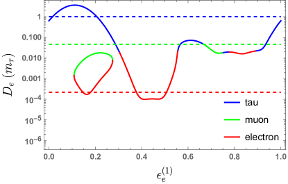
Figure 3: Log plot of the spectrum of eigenvalues of the charged leptons mass as a function of brane position parameter $\epsilon^{(1)}_{e}$ for $\kappa^{(1)}=45$. The dashed colored horizontal lines correspond to the mass eigenvalues of tau, muon and electron $\{1,0.0458,0.000217\}m_{\tau}$ from (149). The exact solution will only be obtained if the respective colored lines touch the dashed grid-lines for a specific value of $\epsilon^{(1)}_{e}$. The nearest-fit is obtained at $\epsilon^{(1)}_{e}=0.206558$ with eigenvalues $\{0.999993,0.0171119,0.00053237\}m_{\tau}$.

Figure 3 shows one such spectrum for the specific value of $\kappa^{(1)}=45$. It can be easily seen that the nearest match is obtained for $\epsilon^{(1)}_{e}=0.206558$,

$$|M_{3e}|=m_{\tau}\left(\begin{array}[]{ccc}0.000526961&-0.00410568&8.71084\times 10^{-9}\\ 0.0000218487&0.0171173&-5.03921\times 10^{-8}\\ -1.99023\times 10^{-9}&9.46941\times 10^{-6}&0.999993\\ \end{array}\right)$$ (156)

with eigenvalues $\{0.999993,0.0171119,0.00053237\}m_{\tau}$, where tau lepton is fitted exactly while the muon’s mass comes out to be only 37% while the electron is about 2.45 times heavier than (149). Notice, that these results are only at the tree-level and there could indeed be other corrections, such as those coming from higher-dimensional operators, which may contribute most greatly to the electron and muon masses since they are lighter.

6 Yukawa couplings from 4-point functions

We now turn our attention to the discussion of four-point functions that affect more greatly to the masses of the lighter fermions. We are looking for four-point interactions such as

$$\phi^{i}_{ab}\phi^{j}_{ca}\phi^{k}_{b^{\prime}c}\phi^{l}_{bb^{\prime}}~{}~{}\mathrm{or}~{}~{}\phi^{i}_{ab}\phi^{j}_{ca}\phi^{k}_{cc^{\prime}}\phi^{l}_{bc^{\prime}}~{},~{}\,$$ (157)

where $\phi^{i}_{xy}$ are the chiral superfields at the intersections between stack $x$ and $y$ D6-branes. The formula for the area of a quadrilateral in terms of its angles and two sides and the solutions of diophantine equations for estimating the multiple areas of the quadrilaterals from non-unit intersection numbers are given in Abel:2003yx ; Abel:2003vv . In addition to these formulae, there is a more intuitive way to calculate the area for these four-sided polygons. A quadrilateral can be always taken as the difference between two similar triangles. Therefore, since we know the classical part is

$$Z_{4cl}\sim e^{-A_{quad}},$$ (158)

it is equivalent to write Chen:2008rx ,

$$Z_{4cl}\sim e^{-|A_{tri}-A^{\prime}_{tri}|}.$$ (159)

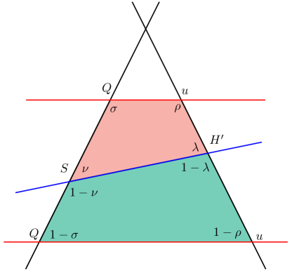
Figure 4: A picture of two quadrilaterals with different field orders. The red brane repeats in a next cycle and can still form a similar quadrilateral with the blue brane. This coupling also contributes to the four-point function.

Taking the absolute value of the difference reveals that there are two cases: $A_{tri}>A^{\prime}_{tri}$ and $A_{tri}<A^{\prime}_{tri}$, as shown in figure 4. From the figure we can see the two quadrilaterals are similar with different sizes, but the orders of the fields corresponding to the angles are different, which is under an interchange of $\theta\leftrightarrow 1-\theta$, $\theta=\nu,\lambda,\rho,\sigma$. These different field orders may cause different values for their quantum contributions. Here, we shall only consider the classical contribution from the 4-point interaction and ignore the quantum part which was shown to be further suppressed, consult Chen:2008rx and references therein for details. Therefore, we are able to employ the same techniques which have developed for calculating the trilinear Yukawa couplings.

For a quadrilateral formed by the stacks $a$, $b$, $b^{\prime}$, $c$, we can calculate it as the difference between two triangles formed by stacks $a$, $b$, $c$ and $b^{\prime}$, $b$, $c$. In other words, they share the same intersection $I_{bc}$. Therefore, if we use this method to calculate the quadrilateral area, we should keep in mind that the intersection index $k$ for $I_{bc}$ remains the same for a certain class of quadrilaterals when varying other intersecting indices. Here we set indices $i$ for $I_{ab}$, $j$ for $I_{ca}$, $\imath$ for $I_{bb^{\prime}}$, and $\jmath$ for $I_{cb^{\prime}}$, as shown in figure 5. We may calculate the areas of the triangles as we did in the trilinear Yukawa couplings above Cremades:2003qj

$$A_{ijk}=\frac{1}{2}(2\pi)^{2}A_{\mathbf{T^{2}}}|I_{ab}I_{bc}I_{ca}|~{}\big{(}\frac{i}{I_{ab}}+\frac{j}{I_{ca}}+\frac{k}{I_{bc}}+\epsilon+l\big{)}^{2},$$

$$A_{\imath\jmath k}=\frac{1}{2}(2\pi)^{2}A_{\mathbf{T^{2}}}|I_{b^{\prime}b}I_{bc}I_{cb^{\prime}}|~{}\big{(}\frac{\imath}{I_{b^{\prime}b}}+\frac{\jmath}{I_{cb^{\prime}}}+\frac{k}{I_{bc}}+\varepsilon+\ell\big{)}^{2},$$ (160)

where $i$, $j$, $k$ and $\imath$, $\jmath$, $k$ are using the same selection rules as Eq. (114). Thus, the classical contribution of the four-point functions is given by

$$Z_{4cl}=\sum_{l,\ell}e^{-\frac{1}{2\pi}|A_{ijk}-A_{\imath\jmath k}|}.$$ (161)

Note that this formula will diverge when $A_{ijk}=A_{\imath\jmath k}$, which is due to over-counting the zero area when the corresponding parameters in Eq. (160) are the same. In such a case, $Z_{4cl}=1+\sum_{l\neq\ell}e^{-\frac{1}{2\pi}|A_{ijk}-A_{\imath\jmath k}|}$. We will not meet this special situation in our following discussion.

We will consider both types of possible interactions (157) coming from considering $b^{\prime}$ or from considering $c^{\prime}$ independently.

6.1 Mass corrections from 4-point functions considering $b^{\prime}$

Figure 5: A diagram showing the areas bounded by stacks of D-branes which give rise to the Yukawa couplings for quarks and leptons via world-sheet instantons. The Yukawa couplings of the up-type quarks are from the areas by stack $a_{1}$, $b$, $c_{1}$, the down-type quarks by stack $a_{1}$, $b$, $c_{2}$, and the leptons by $a_{2}$, $b$, $c_{2}$. The four-point function corrections to the Yukawa couplings of the up-type quarks are from the areas by stack $a_{1}$, $b$, $b^{\prime}$, $c_{1}$, the down-type quarks by stack $a_{1}$, $b$, $b^{\prime}$, $c_{2}$, and the leptons by $a_{2}$, $b$, $b^{\prime}$, $c_{2}$.

In the model of table 3, in addition to the intersection numbers in Eq. (109), we have

$$I_{cb^{\prime}}^{(1)} =1, I_{cb^{\prime}}^{(2)} =-1, I_{cb^{\prime}}^{(3)} =1;$$

$$I_{bb^{\prime}}^{(1)} =20, I_{bb^{\prime}}^{(2)} =0, I_{bb^{\prime}}^{(3)} =-1;$$

$$I_{cc^{\prime}}^{(1)} =-4, I_{cc^{\prime}}^{(2)} =0, I_{cc^{\prime}}^{(3)} =-1;$$ (162)

There are twenty SM singlet fields $S_{L}^{i}$ and one Higgs-like state $H^{\prime}_{u,d}$. Similar to the Higgs fields $H^{i}_{u,d}$, only three linear combinations of the twenty $S_{L}^{i}$ can contribute to the four-point Yukawa couplings. Considering the following parameters with shifts $l=-k/3$ and $\ell=-k/9$ taken along the index $k$,

$$\delta =\frac{i}{I_{ab}^{(1)}}+\frac{j}{I_{ca}^{(1)}}+\frac{k}{I_{bc}^{(1)}}+l,$$

$$=\frac{i}{3}+\frac{j}{3},$$ (163)

$$d =\frac{\imath}{I_{cc^{\prime}}^{(1)}}+\frac{\jmath}{I_{cb^{\prime}}^{(1)}}+\frac{k}{I_{bc}^{(1)}}+\ell,$$

$$=\frac{\imath}{20}+\jmath,$$ (164)

the matrix elements $a_{i,j,\imath}$ on the first torus from the four-point functions can be expressed as

$$\left(\begin{array}[]{ccc}\sum_{i=0}^{6}a_{1,1,3i+1}&\sum_{i=0}^{5}a_{1,2,3i+3}&\sum_{i=0}^{6}a_{1,3,3i+2}\\ \sum_{i=0}^{5}a_{2,1,3i+3}&\sum_{i=0}^{6}a_{2,2,3i+2}&\sum_{i=0}^{6}a_{2,3,3i+1}\\ \sum_{i=0}^{6}a_{3,1,3i+2}&\sum_{i=0}^{6}a_{3,2,3i+1}&\sum_{i=0}^{5}a_{3,3,3i+3}\\ \end{array}\right),$$ (165)

and the classical 4-point contribution to the mass matrix given as,

$$Z_{4cl}=\left(\begin{array}[]{ccc}u_{1}\sum_{i=0}^{6}w_{3i+1}A_{3i}&u_{2}\sum_{i=0}^{5}w_{3i+3}A_{3i+2}&u_{3}\sum_{i=0}^{6}w_{3i+2}A_{3i+1}\\ u_{1}\sum_{i=0}^{5}w_{3i+3}A_{3i+2}&u_{2}\sum_{i=0}^{6}w_{3i+2}A_{3i+1}&u_{3}\sum_{i=0}^{6}w_{3i+1}A_{3i}\\ u_{1}\sum_{i=0}^{6}w_{3i+2}A_{3i+1}&u_{2}\sum_{i=0}^{6}w_{3i+1}A_{3i}&u_{3}\sum_{i=0}^{5}w_{3i+3}A_{3i+2}\\ \end{array}\right),$$ (166)

where $u_{i},w_{j}$ are the VEVs and the couplings are defined as,

$$A_{i}\equiv\vartheta\left[\begin{array}[]{c}\epsilon^{(1)}+\dfrac{i}{20}\\ \phi^{(1)}\end{array}\right](\frac{9J^{(1)}}{\alpha^{\prime}}),\qquad i={0,\dots,|I_{bb^{\prime}}^{(1)}|-1}.$$ (167)

Since, we have already fitted the up-type quark matrix $|M_{3u}|$ exactly, so its 4-point correction should be zero,

$$|M_{4u}|=0,$$ (168)

which is true by setting all up-type VEVs $u_{u}^{i}$ and $w_{u}^{i}$ to be zero. Therefore, we are essentially concerned with fitting charged leptons in such a way that corresponding corrections for the down-type quarks remain negligible. The desired solution can be readily obtained by setting $\epsilon^{(1)}_{4e}=0$ and $\epsilon^{(1)}_{4d}=1/20$ with the following values of the VEVs,

$$\begin{array}[]{lll}u_{d}^{1}=-1/27,&u_{d}^{2}=1,&u_{d}^{3}=1/100,\\ w_{d}^{i}=0,&i={1,\dots,14},&\\ w_{d}^{15}=0.172138,&w_{d}^{16}=0.0858488&w_{d}^{17}=0.0247877,\\ w_{d}^{18}=-0.0000123476,&w_{d}^{19}=-0.0000513328,&w_{d}^{20}=-0.000123552.\\ \end{array}$$ (169)

The 4-point correction to the charged leptons masses is given by,

$$|M_{4e}|=m_{\tau}\left(\begin{array}[]{ccc}-0.000309961&0.000697239&0.000286827\\ -0.0000258237&0.0286827&0.0000836895\\ -0.00106232&0.00836895&6.97239\times 10^{-6}\\ \end{array}\right)$$ (170)

which can be added to the matrix obtained from 3-point functions (156) as,

$$|M_{3e}|+|M_{4e}|=m_{\tau}\left(\begin{array}[]{ccc}0.000217&-0.00340844&0.000286835\\ -3.97501\times 10^{-6}&0.0458&0.0000836391\\ -0.00106232&0.00837842&1.\\ \end{array}\right)$$ (171)

that can be readily diagonalized as,

$$m_{\tau}\left(\begin{array}[]{ccc}0.00217014&0&0\\ 0&0.0457996&0\\ 0&0&1.\\ \end{array}\right)\sim D_{e}~{},$$ (172)

which exactly reproduces the correct masses of all three charged leptons cf. (149). Also, the corrections to down-type quarks are kept to almost zero by setting $\epsilon^{(1)}_{4d}=1/20$,

$$|M_{4d}|\sim 0.$$ (173)

which preserves our previously obtained exact fit using 3-point functions (5.2).

6.2 Mass corrections from 4-point functions considering $c^{\prime}$

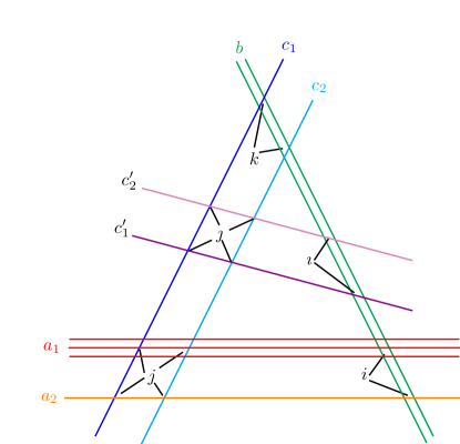
Figure 6: A diagram showing the areas bounded by stacks of D-branes which give rise to the Yukawa couplings for quarks and leptons via world-sheet instantons. The Yukawa couplings of the up-type quarks are from the areas by stack $a_{1}$, $b$, $c_{1}$, the down-type quarks by stack $a_{1}$, $b$, $c_{2}$, and the leptons by $a_{2}$, $b$, $c_{2}$. The four-point function corrections to the Yukawa couplings of the up-type quarks are from the areas by stack $a_{1}$, $b$, $c^{\prime}$, $c_{1}$, the down-type quarks by stack $a_{1}$, $b$, $c^{\prime}$, $c_{2}$, and the leptons by $a_{2}$, $b$, $c^{\prime}$, $c_{2}$.

There are four SM singlet fields $S_{L}^{i}$ and one Higgs-like state $H^{\prime}_{u,d}$. Similar to the Higgs fields $H^{i}_{u,d}$, only three linear combinations of the twenty $S_{L}^{i}$ can contribute to the four-point Yukawa couplings. Considering the following parameters with shifts $l=-k/3$ and $\ell=-k/9$ taken along the index $k$,

$$\delta =\frac{i}{I_{ab}^{(1)}}+\frac{j}{I_{ca}^{(1)}}+\frac{k}{I_{bc}^{(1)}}+l,$$

$$=\frac{i}{3}+\frac{j}{3},$$ (174)

$$d =\frac{\imath}{I_{cc^{\prime}}^{(1)}}+\frac{\jmath}{I_{cb^{\prime}}^{(1)}}+\frac{k}{I_{bc}^{(1)}}+\ell,$$

$$=-\frac{\imath}{4}+\jmath,$$ (175)

the matrix elements $a_{i,j,\imath}$ on the first torus from the four-point functions can be expressed as,

$$\left(\begin{array}[]{ccc}a_{1,1,4}+a_{1,1,1}&a_{1,2,3}&a_{1,3,2}\\ a_{2,1,3}&a_{2,2,2}&a_{2,3,1}+a_{2,3,4}\\ a_{3,1,2}&a_{3,2,1}+a_{3,2,4}&a_{3,3,3}\\ \end{array}\right).$$ (176)

and the classical 4-point contribution to the mass matrix given as,

$$Z_{4cl}=\left(\begin{array}[]{ccc}u_{1}(w_{4}A_{1}+w_{1}A_{0})&u_{2}w_{3}A_{2}&u_{3}w_{2}A_{3}\\ u_{1}w_{3}A_{2}&u_{2}w_{2}A_{3}&u_{3}(w_{4}A_{1}+w_{1}A_{0})\\ u_{1}w_{2}A_{3}&u_{2}(w_{4}A_{1}+w_{1}A_{0})&u_{3}w_{3}A_{2}\\ \end{array}\right),$$ (177)

where $u_{i},w_{j}$ are the VEVs and the couplings are defined as,

$$A_{i}\equiv\vartheta\left[\begin{array}[]{c}\epsilon^{(1)}+\dfrac{i}{4}\\ \phi^{(1)}\end{array}\right](\frac{9J^{(1)}}{\alpha^{\prime}}),\qquad i={0,\dots,|I_{cc^{\prime}}^{(1)}|-1}.$$ (178)

Since, we have already fitted the up-type quark matrix $|M_{3u}|$ exactly, so its 4-point correction should be zero,

$$|M_{4u}|=0,$$ (179)

which is true by setting all up-type VEVs $u_{u}^{i}$ and $w_{u}^{i}$ to be zero. Therefore, we are essentially concerned with fitting charged leptons in such a way that corresponding corrections for the down-type quarks remain negligible. The desired solution can be readily obtained by setting $\epsilon^{(1)}_{4e}=1/4$ and $\epsilon^{(1)}_{4d}=3/4$ with the following values of the VEVs,

$$\begin{array}[]{lll}u_{d}^{1}=-1/27,&u_{d}^{2}=1,&u_{d}^{3}=1/100,\\ w_{d}^{1}=1.8183,&w_{d}^{2}=0.000906372,&\\ w_{d}^{3}=0.151488,&w_{d}^{4}=-0.000264.&\\ \end{array}$$ (180)

The 4-point correction to the charged leptons masses is given by,

$$|M_{4e}|=m_{\tau}\left(\begin{array}[]{ccc}-0.000309961&0.000697239&0.000286827\\ -0.0000258237&0.0286827&0.0000836895\\ -0.00106232&0.00836895&6.97239\times 10^{-6}\\ \end{array}\right),$$ (181)

which can be added to the matrix obtained from 3-point functions (156) as,

$$|M_{3e}|+|M_{4e}|=m_{\tau}\left(\begin{array}[]{ccc}0.000217&-0.00340844&0.000286835\\ -3.97501\times 10^{-6}&0.0458&0.0000836391\\ -0.00106232&0.00837842&1.\\ \end{array}\right),$$ (182)

that can be readily diagonalized as,

$$m_{\tau}\left(\begin{array}[]{ccc}0.00217014&0&0\\ 0&0.0457996&0\\ 0&0&1.\\ \end{array}\right)\sim D_{e}~{},$$ (183)

which exactly reproduces the correct masses of all three charged leptons cf. (149). Also, the corrections to down-type quarks are kept to almost zero by setting $\epsilon^{(1)}_{4d}=3/4$,

$$|M_{4d}|=\left(\begin{array}[]{ccc}-8.49479\times 10^{-7}&0.00110164&0\\ -0.0000408014&0&2.29359\times 10^{-7}\\ 0&0.0000229359&0.0000110164\\ \end{array}\right)\sim 0,$$ (184)

which preserves our previously obtained exact fit using 3-point functions (5.2).

In summary, we can correctly reproduce, the correct masses and mixings of quarks and the masses of charged leptons at the electroweak scale. Finally, by choosing suitable Majorana mass matrix for the right-handed neutrinos the suitable masses of neutrinos and their mixings can be generated by type I seesaw mechanism.

7 Discussion and conclusion

We have studied the phenomenology of a new class of supersymmetric Pati-Salam intersecting D6-brane model on a $\mathbf{T}^{6}/(\mathbb{Z}_{2}\times\mathbb{Z}_{2})$ orientifold in type IIA string theory. The defining characteristic of this new-class is that one of the wrapping numbers is 5 and models exhibit approximate gauge coupling unification. We have discussed the SM fermion masses and mixings and supersymmetry breaking soft terms in the $u$-moduli dominated case and the $u$-moduli dominant case together with the $s$-moduli turned on, where the soft terms remain independent of the Yukawa couplings and the Wilson lines. The results depend on the brane wrapping numbers as well as supersymmetry breaking parameters.

Although we are able to reproduce the extrapolated GUT-scale mass hierarchies and the mixings of the standard model fermions in our intersecting brane model on a IIA orientifold setting exactly, several issues remain to be addressed. The values of various couplings and other parameters are not determined uniquely within the model and are rather put by hand. All such parameters are the functions of open and closed string moduli. For instance the Yukawa couplings depend on the geometric position of the stacks of branes and the Kähler moduli. Once we fix these moduli, the only freedom left is the Higgs sector, i.e. finding a specific linear combination of nine pairs of Higgs states which may be fine-tuned to yield the two Higgs eigenstates $H_{u}$ and $H_{d}$ of the MSSM.

Fixing the brane positions is thus equivalent to fixing the open string moduli. Unless these open string moduli are fixed, the low energy spectrum will contain non-chiral open string states associated to the brane positions and the Wilson lines. We do not see such scalar particles in Nature. Luckily so, otherwise they will also spoil the gauge coupling unification in the MSSM. Therefore, it is tempting to eliminate such non-chiral fields by considering intersecting D-brane models wrapping on rigid cycles. In the case of type II compactifications, $\mathbf{T}^{6}/(\mathbb{Z}_{2}\times\mathbb{Z}^{\prime}_{2})$ is the only known toroidal background possessing such rigid cycles, see ref. Blumenhagen:2005tn for details. This may be explored in a future study.

Appendix A Soft terms from susy breaking for model in ref. Chen:2007zu

Table 6: D6-brane configurations and intersection numbers for the model on Type IIA $\mathbf{T}^{6}/\mathbb{Z}_{2}\times\mathbb{Z}_{2}$ orientifold.

	${\rm U}(4)_{C}\times{\rm U}(2)_{L}\times{\rm U}(2)_{R}\times{\rm USp}(2)^{4}$
	$N$	$(n^{1},l^{1})\times(n^{2},l^{2})\times\par(n^{3},l^{3})$	$n_{S}$	$n_{A}$	$b$	$b^{\prime}$	$c$	$c^{\prime}$	1	2	3	4
$a$	8	$(0,-1)\times(1,1)\times(1,1)$	0	0	3	0	-3	0	1	-1	0	0
$b$	4	$(3,1)\times(1,0)\times(1,-1)$	2	-2	-	-	0	0	0	1	0	-3
$c$	4	$(3,-1)\times(0,1)\times(1,-1)$	-2	2	-	-	-	-	-1	0	3	0
1	2	$(1,0)\times(1,0)\times(2,0)$	$\chi_{1}=3,~{}\chi_{2}=1,~{}\chi_{3}=2$
2	2	$(1,0)\times(0,-1)\times(0,2)$	$\beta^{g}_{1}=-3,~{}\beta^{g}_{2}=-3$
3	2	$(0,-1)\times(1,0)\times(0,2)$	$\beta^{g}_{3}=-3,~{}\beta^{g}_{4}=-3$
4	2	$(0,-1)\times(0,1)\times(2,0)$

Table 6 shows the well-studied previous model with wrapping number up to 3 with exact gauge coupling unification. This model has been extensively discussed in Refs. Chen:2007zu ; Mayes:2013bda ; Mayes:2019isy ; Gemmill:2019kxr ; Li:2014xqa . The gaugino masses, trilinear coupling and the squared masses of sleptons and squarks for this model computed in Li:2014xqa did not take into account the fact that the third torus is tilted. Consequently, there was some discrepancy in the trilinear coupling and the squared sleptons and squarks masses. Below we perform the computation making use of Kronecker deltas and the sign matrix $\sigma^{i}_{xy}$ defined in (73), which conveniently takes into account the signs in the derivative of the angles and the $\Psi$-functions.

From table 6, the complex structure moduli $U$ from (15) can be calculated as,

$$\{U_{1},U_{2},U_{3}\} =\{3i,i,1+i\},$$ (185)

and the corresponding $u$-moduli and $s$-modulus in supergravity basis from (16) are,

$$u_{i} =\{\frac{e^{-\phi_{4}}}{\sqrt{6}\pi},\frac{\sqrt{\frac{3}{2}}e^{-\phi_{4}}}{\pi},\frac{\sqrt{\frac{3}{2}}e^{-\phi_{4}}}{2\pi}\},$$

$$s =\frac{e^{-\phi_{4}}}{2\sqrt{6}\pi}.$$ (186)

Using (21) and the values from the table 6, the gauge kinetic function becomes,

$$f_{x} =\frac{\sqrt{\frac{3}{2}}e^{-\phi_{4}}}{4\pi},\quad{x=a,b,c}.$$ (187)

To calculate gaugino masses $M_{1,2,3}$ respectively for ${\rm U}(1)_{Y}$, ${\rm SU}(2)_{L}$ and ${\rm SU}(3)_{c}$ gauge groups, we first compute $M_{a,b,c}$ using (• ‣ 3.2) as,

$$M_{a} =\frac{\sqrt{3}}{2}m_{3/2}\left(e^{-i\gamma_{2}}\Theta_{3}+e^{-i\gamma_{3}}\Theta_{2}\right),$$

$$M_{b} =\frac{\sqrt{3}}{2}m_{3/2}\left(e^{-i\gamma_{2}}\Theta_{2}-e^{-i\gamma_{4}}\Theta_{4}\right),$$

$$M_{c} =\frac{\sqrt{3}}{2}m_{3/2}\left(e^{-i\gamma_{1}}\Theta_{1}+e^{-i\gamma_{3}}\Theta_{3}\right).$$ (188)

Bino mass parameter $M_{Y}$ (44) is then computed as,

$$M_{Y} =\frac{1}{f_{Y}}(\frac{2}{3}f_{a}M_{a}+f_{c}M_{c})$$

$$=\frac{3\sqrt{3}}{10}m_{3/2}\left(e^{-i\gamma_{1}}\Theta_{1}+\frac{1}{5}e^{-i\gamma_{2}}\Theta_{2}+\frac{1}{2}e^{-i\gamma_{3}}\Theta_{3}\right).$$ (189)

Therefore, the gaugino masses for ${\rm U}(1)_{Y}$, ${\rm SU}(2)_{L}$ and ${\rm SU}(3)_{c}$ gauge groups are,

$$M_{1} \equiv M_{Y}=\frac{3\sqrt{3}}{10}m_{3/2}\left(e^{-i\gamma_{1}}\Theta_{1}+\frac{1}{5}e^{-i\gamma_{2}}\Theta_{2}+\frac{1}{2}e^{-i\gamma_{3}}\Theta_{3}\right),$$

$$M_{2} \equiv M_{b}=\frac{\sqrt{3}}{2}m_{3/2}\left(e^{-i\gamma_{2}}\Theta_{2}-e^{-i\gamma_{4}}\Theta_{4}\right),$$

$$M_{3} \equiv M_{a}=\frac{\sqrt{3}}{2}m_{3/2}\left(e^{-i\gamma_{2}}\Theta_{3}+e^{-i\gamma_{3}}\Theta_{2}\right).$$ (190)

Table 7: The angles (in multiples of $\pi$) with respect to the orientifold plane made by the cycle wrapped by each stack of D-branes on each of the three two-tori.

	$\theta_{1}$	$\theta_{2}$	$\theta_{3}$
$a$	$-1/2$	$\ 1/4$	$1/4$
$b$	$\ 1/4$	$\ 0$	$-1/4$
$c$	$-1/4$	$\ 1/2$	$-1/4$

We now require the angles, the differences of angles and their first and second order derivatives with respect to the moduli to compute the trilinear coupling and the sleptons mass-squared. In table 7 we show the angles made by the cycle wrapped by each stack D6 branes with respect to the orientifold plane in multiples of $\pi$,

$$\theta_{x}^{i} =\frac{1}{\pi}\tan^{-1}\left(\frac{2^{-\beta_{i}}l_{x}^{i}\chi_{i}}{n_{x}^{i}}\right).$$ (191)

The differences of the angles are,

$$\theta_{y}^{i}-\theta_{x}^{i}\equiv\theta_{xy}^{i}=\left(\begin{array}[]{ccc}\{0,0,0\}&\left\{\frac{3}{4},-\frac{1}{4},-\frac{1}{2}\right\}&\left\{\frac{1}{4},\frac{1}{4},-\frac{1}{2}\right\}\\ \left\{-\frac{3}{4},\frac{1}{4},\frac{1}{2}\right\}&\{0,0,0\}&\left\{-\frac{1}{2},\frac{1}{2},0\right\}\\ \left\{-\frac{1}{4},-\frac{1}{4},\frac{1}{2}\right\}&\left\{\frac{1}{2},-\frac{1}{2},0\right\}&\{0,0,0\}\\ \end{array}\right).$$ (195)

To account for the negative angle differences we make use of the $\sigma_{xy}^{i}$ function (73) which is $-1$ only for negative angle difference and $+1$ otherwise,

$$\sigma_{xy}^{i}\equiv(-1)^{1-H(\theta_{xy}^{i})} =\left(\begin{array}[]{ccc}\{1,1,1\}&\{-1,-1,1\}&\{1,-1,1\}\\ \{1,1,-1\}&\{1,1,1\}&\{1,-1,1\}\\ \{-1,1,-1\}&\{-1,1,1\}&\{1,1,1\}\\ \end{array}\right),$$ (199)

where $H(x)$ is the unit step function. And the function $\eta_{xy}$ can thus be defined by taking the product on the torus index $i$ as,

$$\eta_{xy}\equiv\prod_{i}\sigma_{xy}^{i}=\left(\begin{array}[]{ccc}1&1&-1\\ -1&1&-1\\ 1&-1&1\\ \end{array}\right).$$ (200)

Using above defined $\sigma_{xy}^{i}$ and $\eta_{xy}^{i}$, we can readily write the four cases of functions $\Psi(\theta_{xy})$ defined in (48) and (49) into a single expression as,

$$\Psi(\theta^{j}_{xy}) =\eta_{xy}\left(\frac{1}{2}\psi^{(0)}(\sigma_{xy}^{i}\theta^{j}_{xy})+\frac{1}{2}\psi^{(0)}(1-\sigma_{xy}^{i}\theta^{j}_{xy})+\gamma_{E}-\log(t^{j}+\bar{t}^{j})\right),$$ (201)

where $\psi^{(0)}(z)$ is called the digamma function defined as the derivative of the logarithm of the gamma function. The successive derivatives of the $\log\Gamma(z)$ yield the polygamma function $\psi^{(n)}(z)$ as,

$$\psi^{(n-1)}(z)=\frac{d^{(n)}}{dz^{(n)}}\log\Gamma(z),$$ (202)

with the following properties,

$$\frac{d}{dz}\psi^{(0)}(\pm z) =\pm\psi^{(1)}(\pm z),$$

$$\frac{d}{dz}\psi^{(0)}(1\pm z) =\pm\psi^{(1)}(1\pm z).$$ (203)

Similarly, the derivative $\Psi^{\prime}(\theta^{j}_{xy})=\frac{d\Psi(\theta^{j}_{xy})}{d\theta^{j}_{xy}}$ can be expressed succinctly as,

$$\Psi^{\prime}(\theta^{j}_{xy}) =\eta_{xy}\sigma_{xy}^{i}\left(\frac{1}{2}\psi^{(1)}(\sigma_{xy}^{i}\theta^{j}_{xy})+\frac{1}{2}\psi^{(1)}(1-\sigma_{xy}^{i}\theta^{j}_{xy})\right),$$ (204)

where we have utilized the property (A) and have neglected the contribution of the $t$-moduli.

Lastly, by making use of appropriate Kronecker deltas and defining $u^{4}\equiv s$, we can express the various cases of the first and second derivatives of the angles as,

$${\theta}^{i,m}_{xy}\equiv(u^{m}+\bar{u}^{m})\,\frac{\partial\theta^{i}_{xy}}{\partial u^{m}}=(-1)^{\delta_{m,4}}(-1)^{\delta_{i,j}}\frac{\sin(2\pi\theta^{i})}{4\pi}\bigg{|}^{x}_{y},$$

$$i={1,2,3};\quad m={1,2,3,4.}$$ (205)

$${\theta}^{i,mn}_{xy} \equiv(u^{m}+\bar{u}^{m})(u^{n}+\bar{u}^{n})\,\frac{\partial^{2}\theta^{i}_{xy}}{\partial u^{m}\partial\bar{u}^{n}}$$

$$=\delta_{m,n}\frac{\sin(4\pi\theta^{i})+(-1)^{(1-\delta_{4,m})(1-\delta_{i,m})}4\sin(2\pi\theta^{i})}{16\pi}\bigg{|}^{x}_{y}$$

$$\quad+(1-\delta_{m,n})(-1)^{(1-\delta_{4,m})(1-\delta_{4,n})(\delta_{i,m}+\delta_{i,n})}(-1)^{1-\delta_{i,m}-\delta_{i,n}}\frac{\sin(4\pi\theta^{i})}{16\pi}\bigg{|}^{x}_{y},$$

$$\qquad\qquad\qquad\qquad\qquad\qquad\qquad\qquad i={1,2,3};\quad m,n={1,2,3,4}.$$ (206)

Substituting above results in (• ‣ 3.2) and ignoring the CP-violating phases $\gamma^{i}$, we obtain the following the trilinear couplings,

$$A_{0} \equiv A_{abc}=A_{acb}=\frac{\sqrt{3}m_{3/2}}{4\pi}\Bigg{[}-\Theta_{1}\left(2\pi+2\gamma_{E}+\psi^{(0)}\left(\frac{1}{4}\right)+\psi^{(0)}\left(\frac{3}{4}\right)\right)$$

$$\quad+\Theta_{2}\left(-2\pi+2\gamma_{E}+\psi^{(0)}\left(\frac{1}{4}\right)+\psi^{(0)}\left(\frac{3}{4}\right)\right)$$

$$\quad+\Theta_{3}\left(2\gamma_{E}+\psi^{(0)}\left(\frac{1}{4}\right)+\psi^{(0)}\left(\frac{3}{4}\right)\right)-\Theta_{4}\left(2\gamma_{E}+\psi^{(0)}\left(\frac{1}{4}\right)+\psi^{(0)}\left(\frac{3}{4}\right)\right)\Bigg{]}.$$ (207)

Ignoring the CP-violating phases $\gamma^{i}$, the gaugino masses, trilinear coupling and sleptons and squarks mass-squared (• ‣ 3.2) parameters are obtained as,

$$M_{1} =m_{3/2}(0.519615\Theta_{1}+0.34641\Theta_{2}+0.866025\Theta_{3}),$$

$$M_{2} =m_{3/2}(0.866025\Theta_{2}-0.866025\Theta_{4}),$$

$$M_{3} =m_{3/2}(0.866025\Theta_{2}+0.866025\Theta_{3}),$$

$$A_{0} =m_{3/2}(-0.292797\Theta_{1}-1.43925\Theta_{2}-0.573228\Theta_{3}+0.573228\Theta_{4}),$$

$$m^{2}_{ab} \equiv m^{2}_{L}=m_{3/2}{}^{2}\Big{(}1-2.02977\Theta_{1}{}^{2}+0.75\Theta_{1}\Theta_{2}-1.5\Theta_{1}\Theta_{4}-0.0440466\Theta_{2}{}^{2}-1.5\Theta_{2}\Theta_{3}$$

$$\quad\quad\quad+0.286907\Theta_{3}{}^{2}+0.75\Theta_{3}\Theta_{4}+0.286907\Theta_{4}{}^{2}\Big{)},$$

$$m^{2}_{ac} \equiv m^{2}_{R}=m_{3/2}{}^{2}\Big{(}1-0.0880932\Theta_{1}{}^{2}-1.5\Theta_{1}\Theta_{2}+0.75\Theta_{1}\Theta_{3}+0.75\Theta_{1}\Theta_{4}-0.0880932\Theta_{2}{}^{2}$$

$$\quad\quad\quad+0.75\Theta_{2}\Theta_{3}+0.75\Theta_{2}\Theta_{4}-0.419047\Theta_{3}{}^{2}-1.5\Theta_{3}\Theta_{4}-2.40477\Theta_{4}{}^{2}\Big{)}.$$ (208)

All above results are subject to the constraint,

$$\sum_{i=1}^{4}\Theta_{i}^{2}=1.$$ (209)

References

- (1) C.-M. Chen, T. Li, V. E. Mayes and D. V. Nanopoulos, Towards realistic supersymmetric spectra and Yukawa textures from intersecting branes, Phys. Rev. D 77 (2008) 125023 [0711.0396].
- (2) E. Witten, Quest for unification, in 10th International Conference on Supersymmetry and Unification of Fundamental Interactions (SUSY02), pp. 604–610, 7, 2002, hep-ph/0207124.
- (3) N. Chamoun, S. Khalil and E. Lashin, Fermion masses and mixing in intersecting branes scenarios, Phys. Rev. D 69 (2004) 095011 [hep-ph/0309169].
- (4) T. Higaki, N. Kitazawa, T. Kobayashi and K.-j. Takahashi, Flavor structure and coupling selection rule from intersecting D-branes, Phys. Rev. D 72 (2005) 086003 [hep-th/0504019].
- (5) M. Cvetic, T. Li and T. Liu, Supersymmetric Pati-Salam models from intersecting D6-branes: A Road to the standard model, Nucl. Phys. B 698 (2004) 163 [hep-th/0403061].
- (6) T. Li, A. Mansha and R. Sun, Revisiting the supersymmetric Pati–Salam models from intersecting D6-branes, Eur. Phys. J. C 81 (2021) 82 [1910.04530].
- (7) E. G. Gimon and J. Polchinski, Consistency conditions for orientifolds and D-manifolds, Phys. Rev. D 54 (1996) 1667 [hep-th/9601038].
- (8) M. B. Green and J. H. Schwarz, Anomaly Cancellation in Supersymmetric D=10 Gauge Theory and Superstring Theory, Phys. Lett. B 149 (1984) 117.
- (9) E. Witten, D-branes and K-theory, JHEP 12 (1998) 019 [hep-th/9810188].
- (10) J. F. G. Cascales and A. M. Uranga, Chiral 4d string vacua with D branes and NSNS and RR fluxes, JHEP 05 (2003) 011 [hep-th/0303024].
- (11) F. Marchesano and G. Shiu, MSSM vacua from flux compactifications, Phys. Rev. D 71 (2005) 011701 [hep-th/0408059].
- (12) F. Marchesano and G. Shiu, Building MSSM flux vacua, JHEP 11 (2004) 041 [hep-th/0409132].
- (13) A. M. Uranga, D-brane probes, RR tadpole cancellation and K-theory charge, Nucl. Phys. B 598 (2001) 225 [hep-th/0011048].
- (14) C.-M. Chen, T. Li and D. V. Nanopoulos, Type IIA Pati-Salam flux vacua, Nucl. Phys. B 740 (2006) 79 [hep-th/0601064].
- (15) M. Cvetic, P. Langacker, T.-j. Li and T. Liu, D6-brane splitting on type IIA orientifolds, Nucl. Phys. B 709 (2005) 241 [hep-th/0407178].
- (16) M. Cvetic, R. Richter and T. Weigand, Computation of D-brane instanton induced superpotential couplings: Majorana masses from string theory, Phys. Rev. D 76 (2007) 086002 [hep-th/0703028].
- (17) R. Blumenhagen, M. Cvetic and T. Weigand, Spacetime instanton corrections in 4D string vacua: The Seesaw mechanism for D-Brane models, Nucl. Phys. B 771 (2007) 113 [hep-th/0609191].
- (18) M. Haack, D. Krefl, D. Lust, A. Van Proeyen and M. Zagermann, Gaugino Condensates and D-terms from D7-branes, JHEP 01 (2007) 078 [hep-th/0609211].
- (19) B. Florea, S. Kachru, J. McGreevy and N. Saulina, Stringy Instantons and Quiver Gauge Theories, JHEP 05 (2007) 024 [hep-th/0610003].
- (20) E. Cremmer, S. Ferrara, L. Girardello and A. Van Proeyen, Yang-Mills Theories with Local Supersymmetry: Lagrangian, Transformation Laws and SuperHiggs Effect, Nucl. Phys. B 212 (1983) 413.
- (21) D. Lust, P. Mayr, R. Richter and S. Stieberger, Scattering of gauge, matter, and moduli fields from intersecting branes, Nucl. Phys. B 696 (2004) 205 [hep-th/0404134].
- (22) G. L. Kane, P. Kumar, J. D. Lykken and T. T. Wang, Some phenomenology of intersecting D-brane models, Phys. Rev. D 71 (2005) 115017 [hep-ph/0411125].
- (23) R. Blumenhagen, B. Kors, D. Lust and S. Stieberger, Four-dimensional String Compactifications with D-Branes, Orientifolds and Fluxes, Phys. Rept. 445 (2007) 1 [hep-th/0610327].
- (24) I. R. Klebanov and E. Witten, Proton decay in intersecting D-brane models, Nucl. Phys. B 664 (2003) 3 [hep-th/0304079].
- (25) R. Blumenhagen, D. Lust and S. Stieberger, Gauge unification in supersymmetric intersecting brane worlds, JHEP 07 (2003) 036 [hep-th/0305146].
- (26) L. E. Ibanez, F. Marchesano and R. Rabadan, Getting just the standard model at intersecting branes, JHEP 11 (2001) 002 [hep-th/0105155].
- (27) R. Blumenhagen, M. Cvetic, F. Marchesano and G. Shiu, Chiral D-brane models with frozen open string moduli, JHEP 03 (2005) 050 [hep-th/0502095].
- (28) A. Font and L. E. Ibanez, SUSY-breaking soft terms in a MSSM magnetized D7-brane model, JHEP 03 (2005) 040 [hep-th/0412150].
- (29) M. Cvetic and I. Papadimitriou, Conformal field theory couplings for intersecting D-branes on orientifolds, Phys. Rev. D 68 (2003) 046001 [hep-th/0303083].
- (30) Y. Kawamura, T. Kobayashi and T. Komatsu, Specific scalar mass relations in SU(3) x SU(2) x U(1) orbifold model, Phys. Lett. B 400 (1997) 284 [hep-ph/9609462].
- (31) Z. Komargodski and N. Seiberg, Comments on the Fayet-Iliopoulos Term in Field Theory and Supergravity, JHEP 06 (2009) 007 [0904.1159].
- (32) A. Brignole, L. E. Ibanez and C. Munoz, Soft supersymmetry breaking terms from supergravity and superstring models, Adv. Ser. Direct. High Energy Phys. 18 (1998) 125 [hep-ph/9707209].
- (33) A. Brignole, L. E. Ibanez and C. Munoz, Towards a theory of soft terms for the supersymmetric Standard Model, Nucl. Phys. B 422 (1994) 125 [hep-ph/9308271].
- (34) G. Aldazabal, S. Franco, L. E. Ibanez, R. Rabadan and A. M. Uranga, Intersecting brane worlds, JHEP 02 (2001) 047 [hep-ph/0011132].
- (35) D. Cremades, L. E. Ibanez and F. Marchesano, Yukawa couplings in intersecting D-brane models, JHEP 07 (2003) 038 [hep-th/0302105].
- (36) H. Fusaoka and Y. Koide, Updated estimate of running quark masses, Phys. Rev. D 57 (1998) 3986 [hep-ph/9712201].
- (37) G. Ross and M. Serna, Unification and fermion mass structure, Phys. Lett. B 664 (2008) 97 [0704.1248].
- (38) S. A. Abel and A. W. Owen, N point amplitudes in intersecting brane models, Nucl. Phys. B 682 (2004) 183 [hep-th/0310257].
- (39) S. A. Abel and A. W. Owen, Interactions in intersecting brane models, Nucl. Phys. B 663 (2003) 197 [hep-th/0303124].
- (40) C.-M. Chen, T. Li, V. E. Mayes and D. V. Nanopoulos, Yukawa Corrections from Four-Point Functions in Intersecting D6-Brane Models, Phys. Rev. D 78 (2008) 105015 [0807.4216].
- (41) V. E. Mayes, Universal Soft Terms in the MSSM on D-branes, Nucl. Phys. B 877 (2013) 401 [1305.2842].
- (42) V. E. Mayes, All Fermion Masses and Mixings in an Intersecting D-brane World, Nucl. Phys. B 950 (2020) 114848 [1902.00983].
- (43) J. Gemmill, E. Howington and V. E. Mayes, Fitting neutrino masses in a realistic intersecting D-braneworld, Phys. Rev. D 100 (2019) 115048 [1907.07106].
- (44) T. Li, D. V. Nanopoulos, S. Raza and X.-C. Wang, A Realistic Intersecting D6-Brane Model after the First LHC Run, JHEP 08 (2014) 128 [1406.5574].