OU-HEP-220204

Radiative natural supersymmetry
emergent from the string landscape
Howard Baer^1,2, Vernon Barger², Dakotah Martinez¹ and Shadman Salam^1
1Homer L. Dodge Department of Physics and Astronomy, University of Oklahoma, Norman, OK 73019, USA
²Department of Physics, University of Wisconsin, Madison, WI 53706 USA

In string theory with flux compactifications, anthropic selection for structure formation from a discretuum of vacuum energy values provides at present our only understanding of the tiny yet positive value of the cosmological constant. We apply similar reasoning to a toy model of the multiverse restricted to vacua with the MSSM as the low energy effective theory. Here, one expects a statistical selection favoring large soft SUSY breaking terms leading to a derived value of the weak scale in each pocket universe (with appropriate electroweak symmetry breaking) which differs from the weak scale as measured in our universe. In contrast, the SUSY preserving $\mu$ parameter is selected uniformly on a log scale as is consistent with the distribution of SM fermion masses: this favors smaller values of $\mu$. An anthropic selection of the weak scale to within a factor of a few of our measured value– in order to produce complex nuclei as we know them (atomic principle)– provides statistical predictions for Higgs and sparticle masses in accord with LHC measurements. The statistical selection then more often leads to (radiatively-driven) natural SUSY models over the Standard Model or finely-tuned SUSY models such as mSUGRA/CMSSM, split, mini-split, spread, high scale or PeV SUSY. The predicted Higgs and superparticle spectra might be testable at HL-LHC or ILC via higgsino pair production but is certainly testable at higher energy hadron colliders with $\sqrt{s}\sim 30-100$ TeV.

1 Introduction

How can it be that the vacuum energy density $\rho_{vac}=\Lambda_{cc}c^{2}/8\pi G_{N}=\Lambda_{cc}m_{P}^{2}\sim(0.003\ {\rm eV})^{4}$ is more than 120 orders of magnitude below its expected value from quantum gravity? Weinberg suggested that in an eternally inflating multiverse[1, 2] with each pocket universe (PU) supporting its own non-zero value of the cosmological constant (CC) $\Lambda_{cc}$, and with $\Lambda_{cc}$ being distributed across the decades of allowed values, the value of $\Lambda_{cc}$ ought to be no larger than the critical value for which large scale structure, which is required for life as we know it to emerge. This allowed Weinberg to predict the value of $\Lambda_{cc}$ to a factor of several over a decade before it was observed[3, 4].

Weinberg’s prediction relied on environmental selection of a fundamental constant of nature. His solution to the CC problem found a home in a more nuanced understanding of string theory vacuum states[5]. In compactified string theory, one expects the emergence of a visible sector containing the Standard Model (SM) along with a variety of hidden sectors and a large assortment of moduli fields: gravitationally coupled scalar fields that determine the size and shape of the compactified manifold and whose vacuum expectation values determine most of the parameters of the $4-d$ low energy effective field theory (EFT). In realistic flux compactifications of type IIB string theories[6], a common estimate for the number of distinct (metastable) vacua can range up to $10^{500-1000}$[7], and even more for $F$-theory compactifications[8]. These vacua, each with its own $4-d$ EFT and value for $\Lambda_{cc}$, are more than enough to support Weinberg’s solution to the CC problem.

While string theory contains only one scale, the string scale $m_{s}$, Weinberg’s solution provides a mechanism for the emergence of a new scale, $\Lambda_{cc}\ll m_{s}$ via environmental (or anthropic) selection. This result obtains from the expected CC probability distribution

$$dN_{vac}\sim f_{cc}\cdot f_{structure}\cdot d\Lambda_{cc}$$ (1)

where $dN_{vac}$ is the differential distribution of vacua in terms of the cosmological constant. Weinberg assumed the distribution $f_{cc}(\Lambda_{cc})$ was uniformly distributed in the vicinity of $10^{-120}m_{P}^{2}$. Also, $f_{structure}(\Lambda_{cc})$ had the form of a step function $f_{structure}\sim\Theta(10^{-120}m_{P}^{2}-\Lambda_{cc})$ such that values of $\Lambda_{cc}$ too much bigger than our (to be) observed value would lead to too rapid cosmological expansion so that structure in the form of condensing galaxies (and hence stars and planets) would not form, and hence observors would not arise.

Can similar reasoning be applied to the origin of other scales such as the weak scale? Indeed, Agrawal et al.[9, 10] (ABDS) addressed this question in 1998. They found that– in order to allow the formation of complex nuclei, and hence atoms as we know them which seem essential for life to emerge– the allowed values of the weak scale are located within a rather narrow window of values (the ABDS window). Our measured value of $m_{weak}\sim m_{W,Z,h}$ seems to be centrally located within the ABDS window which extends roughly from $0.5m_{weak}^{OU}-(2-5)m_{weak}^{OU}$, where $m_{weak}^{OU}$ is the measured value of the weak scale in our universe.

In the case of the SM, with Higgs potential $V_{Higgs}=-\mu_{SM}^{2}(\phi^{\dagger}\phi)+\lambda(\phi^{\dagger}\phi)^{2}$, with $\lambda>0$ to ensure stability of the Higgs vev, then one might expect

$$dN_{vac}\sim f_{\mu}(\mu_{SM})\cdot f_{ABDS}(\mu_{SM}).$$ (2)

If one assumes all scales of $\mu_{SM}$ equally likely, then $f_{\mu}\sim 1/\mu_{SM}$. Meanwhile, if the PU value of the weak scale $m_{weak}^{PU}\gtrsim(2-5)m_{weak}^{OU}$ (where $OU$ refers to the measured value in our universe), then the up-down quark mass difference would grow to such an extent that neutrons would no longer be stable within nuclei. Consequently, nuclei consisting of multiple protons would no longer be stable (too much Coulumb repulsion), and the only stable nuclei would consist of single proton states: the universe would be chemically sterile and life as we know it would not arise. This argument has been used as an alternative to the usual naturalness argument in that using anthropic reasoning, then the SM might well be valid all the way up to huge scales $Q\sim m_{GUT}-m_{s}$[11] in spite of the presence of quadratic divergences in the Higgs boson mass-squared.

Environmental selection can also be applied to supersymmetric models wherein the Higgs mass-squared contains only logarithmic divergences. Indeed it is emphasized in Ref. [12] that in a landscape containing comparable numbers of SM-like and weak scale SUSY-like low energy EFTs, then the anthropically allowed SUSY models should be much more prevalent because there should be a far wider range of natural parameter choices available compared to the finetuned values which are required for the SM. For SUSY models, we expect a distribution of soft term values according to

$$dN_{vac}\sim f_{SUSY}(m_{soft})\cdot f_{EWSB}\cdot dm_{soft}$$ (3)

For the soft term distribution $f_{SUSY}(m_{soft})$, positive power law[13, 14, 15, 16] or log[17] distributions pull soft terms to large values and seem favored by LHC SUSY search results[18, 19, 17, 20]. In contrast, negative power law distributions, as expected in dynamical SUSY breaking where all SUSY breaking scales would be equally favored[21, 22, 23], or large-volume scenario (LVS) compactifications[16]would lead to sparticle masses below LHC limits and light Higgs boson masses much lighter than the measured value $m_{h}\sim 125$ GeV[24].

The anthropic selection function $f_{EWSB}$ requires that the derived value of the weak scale in each pocket universe

$$m_{Z}^{PU2}/2=\frac{m_{H_{d}}^{2}+\Sigma_{d}^{d}-(m_{H_{u}}^{2}+\Sigma_{u}^{u})\tan^{2}\beta}{\tan^{2}\beta-1}-\mu^{2}$$ (4)

lies within the ABDS window. Thus, one must veto MSSM-like pocket universes wherein $m_{Z}^{PU}>(2-5)m_{Z}^{OU}$ where $m_{Z}^{OU}=91.2$ GeV is the value of $m_{Z}$ in our universe. Assuming no finetuning of the values entering the right-hand-side of Eq. 4, then conventional sparticle and Higgs mass generators such as Isajet[25] and others[26] can be used to make landscape predictions for sparticle and Higgs boson masses. Without finetuning, then the pocket universe value for the weak scale will typically be the maximal entry on the RHS of Eq. 4. Then, requiring $m_{Z}^{PU}\lesssim 4m_{Z}^{OU}$ is the same as requiring the electroweak naturalness measure $\Delta_{EW}\lesssim 30$ (where $\Delta_{EW}\equiv|maximal\ term\ on\ RHS\ of\ Eq.~{}\ref{eq:mzsPU}|/m_{Z}^{OU2}/2$)[19, 27]. Coupling the ABDS requirement with a mild log or power-law draw to large soft terms, then the probability distributions for sparticle and Higgs masses can be computed. It has then been found that the light Higgs mass distribution $dP/dm_{h}$ rises to a peak at $m_{h}\sim 125$ GeV whilst sparticle masses are lifted beyond present LHC search limits[18, 19, 17, 20] (see Ref. [28] for a recent review).

A drawback to the above approach is that it doesn’t allow for accidental (finetuned) parameter values conspiring to create $m_{Z}^{PU}\neq m_{Z}^{OU}$ values which nonetheless end up lying within the ABDS window. This is because the spectrum generators all have the measured value of $m_{Z}$ hardwired into their electroweak symmetry breaking conditions. In the present paper, we build a toy computer code which should provide a better simulation as to what is thought to occur within the multiverse in the case where a subset of vacua containing the minimal supersymmetric standard model (MSSM) is required to be the low energy EFT. This approach allows us to display whether natural SUSY models or finetuned SUSY models are more likely to arise from the landscape. The natural SUSY models are characterized by low $\Delta_{EW}\lesssim 30$ while finetuned SUSY models include the constrained MSSM (CMSSM or mSUGRA model)[32], minisplit SUSY[33, 34], PeV SUSY[35], high scale SUSY[36], spread SUSY[37] and the G2MSSM[38].

In Sec. 2, we discuss our assumed SUSY model and low energy EFT framework. In Sec. 3, we review expectations for the landscape soft term distribution $f_{SUSY}(m_{soft})$ and why it favors large over small soft SUSY breaking terms. We also discuss the assumed distribution for the SUSY $\mu$ parameter. In Sec. 4, we review the crucial anthropic condition that surviving SUSY models lie within the ABDS window, i.e. that the pocket universe value of the weak scale is not-too-far displaced from the value of $m_{weak}$ in our universe. In Sec. 5, we describe our toy model simulation of the multiverse with varying values of $m_{weak}^{PU}$. In Sec. 6, we present results for natural SUSY models and compare them to results from unnatural SUSY models, and explain why natural SUSY is more likely to emerge from anthropic selection within the string landscape than unnatural SUSY models. The answer is that there exists a substantial hypercube of parameter values leading to $m_{weak}^{PU}\lesssim 4m_{weak}^{OU}$ for natural SUSY models while the hypercube shrinks to relatively tiny volume for finetuned models: basically, finetuning of parameters implies that only a tiny sliver of parameter choices are likely to be phenomenologically (anthropically) allowed. Some discussion and conclusions are presented in Sec. 7.

2 SUSY model

In our present discussion, we will adopt the 2-3-4 extra parameter non-universal Higgs model (NUHM2,3,4) for explicit calculations. In this model, the matter scalars of the first two generations are assumed to live in the 16-dimensional spinor of $SO(10)$ as is expected in string models exhibiting local grand unification, where different gauge groups are present at different locales on the compactified manifold[39]. In this case, it is really expected that each generation acquires a different soft breaking mass $m_{0}(1)$, $m_{0}(2)$ and $m_{0}(3)$. But for simplicity of presentation, sometimes we will assume generational degeneracy. At first glance, one might expect that the generational non-degeneracy would lead to violation of flavor-changing-neutral-current (FCNC) bounds. The FCNC bounds mainly apply to first-second generation nonuniversality[40]. However, the landscape itself allows a solution to the SUSY flavor problem in that it statistically pulls all generations to large values provided they do not contribute too much to $m_{weak}^{PU}$. This means the 3rd generation is pulled to $\sim$ several TeV values whilst first and second generation scalars are pulled to values in the $10-50$ TeV range. The first and second generation scalar contributions to the weak scale are suppressed by their small Yukawa couplings[27], whilst their $D$-term contributions largely cancel under intra-generational universality[41]. Their main influence on the weak scale then comes from two-loop RGE contributions which, when large, suppress third generation soft term running leading to tachyonic stop soft terms and possible charge-or-color breaking (CCB) vacua which we anthropically veto[42, 43]. These latter bounds are flavor independent so that first/second generation soft terms are pulled to common upper bounds leading to a quasi-degeneracy/decoupling solution to both the SUSY flavor and CP problems[44]. Meanwhile, Higgs multiplets which live in different GUT representations are expected to have independent soft masses $m_{H_{u}}$ and $m_{H_{d}}$. Thus, we expect a parameter space of the NUHM models as

$$m_{0}(1)\sim m_{0}(2),\ m_{0}(3),\ m_{H_{u}},\ m_{H_{d}},\ m_{1/2},\ A_{0},\ B\mu,\ {\rm and}\ \mu.$$ (5)

We assume that only models with appropriate electroweak symmetry breaking (EWSB) are anthropically allowed (thus generating the weak scale), and the scalar potential minimization conditions allow us to trade $B\mu$ for $\tan\beta$. It is common practise to then finetune either $\mu$ or $m_{H_{u}}$ so as to generate $m_{Z}^{OU}=91.2$ GeV. But it is important that here we do not invoke this condition since we wish to allow $m_{Z}^{PU}$ to float to whatever its derived value takes in the multiverse simulation. For instance, the predicted value of $m_{Z}^{PU}$ from scans over the NUHM3 and NUHM4 models is shown in Fig. 1. We also show the ABDS window (shaded green in the Figure). The vast majority of models would be excluded since they lie beyond the ABDS window (much like the vast majority of $\Lambda_{cc}$ in Weinberg’s explanation of the cosmological constant).

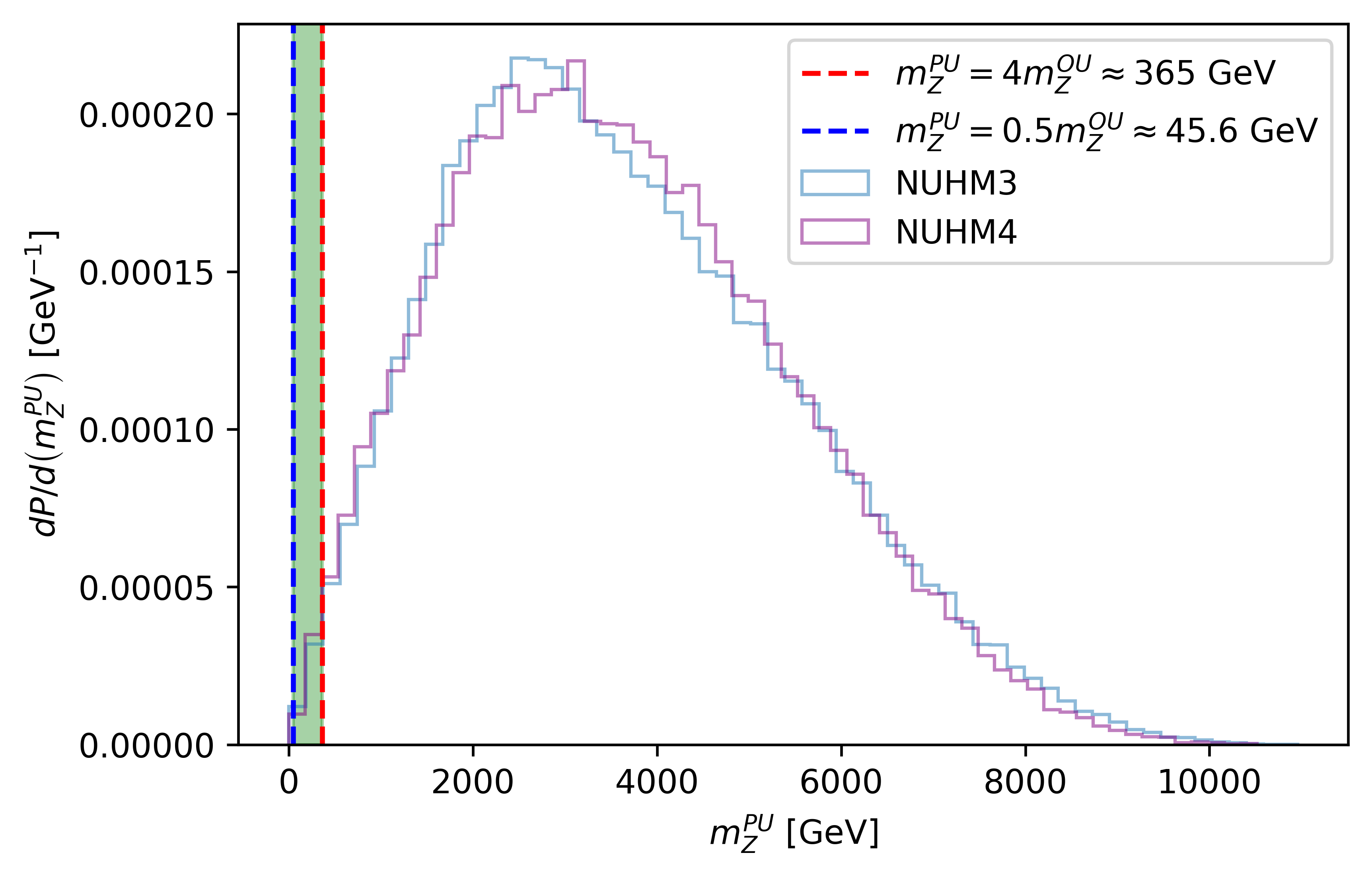
Figure 1: The predicted value of $m_{Z}^{PU}$ from scans over the NUHM3 and NUHM4 models if one doesn’t fine-tune parameters to fix $m_{Z}^{PU}=m_{Z}^{OU}$. The green shaded band is the ABDS window.

3 Distribution of soft terms and $\mu$ parameter on the landscape

3.1 Soft terms

How are the SUSY breaking soft terms expected to be distributed on the landscape? This information would be included in the landscape probability function $f_{SUSY}(m_{soft})$. A variety of proposals have been presented. In Ref’s [13, 14, 15], a power-law draw

$$f_{SUSY}\sim m_{soft}^{2n_{F}+n_{D}-1}$$ (6)

is expected where $n_{F}$ is the number of $F$-breaking fields and $n_{D}$ is the number of $D$-breaking fields contributing to the overall SUSY breaking scale $m_{soft}\sim m_{SUSY}^{2}/m_{P}$ where under gravity-mediation we also expect the gravitino mass $m_{3/2}\sim m_{SUSY}^{2}/m_{P}$. The above form for $f_{SUSY}$ arises if the SUSY breaking $F_{i}$ terms are distributed independently as complex numbers on the landscape whilst the $D$-breaking fields $D_{j}$ are distributed as real random numbers. Subsequently, it was then realized that the sources of SUSY breaking should not be all independent which might spoil the above simplistic expectation[46]. However, even under the condition of single $F$-term source of SUSY breaking, then there is still a linear draw to large soft terms $f_{SUSY}\sim m_{soft}^{1}$. Furthermore, in Ref. [16], under considerations of Kähler moduli stabilization, then a linear distribution $f_{SUSY}\sim m_{soft}^{1}$ would emerge from KKLT[47]-type moduli-stabilization. In contrast, under dynamical SUSY breaking via e.g. gaugino condensation[48] or instanton effects[49], all SUSY breaking scales are expected to be equally probable leading to a distribution $f_{SUSY}\sim m_{soft}^{-1}$[21, 22, 23]. This distribution is also expected to emerge from LVS-type[50] moduli-stabilization[16]. This distribution favors smaller soft terms and leads to sparticle masses below LHC search limits and $m_{h}\ll 125$ GeV[24] and so we will not consider it further here.

A final consideration is whether all soft terms should have common probability distributions on the landscape[51]. For instance, gaugino masses arise from the SUGRA gauge kinetic function $f_{AB}$ which is typically of the form $\sim k\cdot S\delta_{AB}$ in string models where $S$ is the dilaton superfield and $k$ is some constant. Under Eq. 6, then this would give a linear draw to large $m_{1/2}$ while scalar masses which arise from the Kähler function might have a stronger draw to large values. In addition, the other soft terms such as $A_{0}$ have very different dependencies on SUSY breaking fields and hence are expected to scan independently on the landscape[51]. For the bulk of this work, we will generally assume a single source of SUSY breaking so all soft terms scan linearly in $m_{soft}$ to large values.

3.2 $\mu$ term

Since in this work we do not finetune the $\mu$ parameter to gain the measured value of $m_{Z}^{OU}$, we must also be concerned with the expected distribution $f_{\mu}(\mu)$. In solutions to the SUSY $\mu$ problem[52], it is usually expected that the $\mu$ term arises from SUSY breaking via Kähler potential terms such as Giudice-Masiero[53] (GM) operators (wherein $\mu$ is expected to scan as do the soft terms) or via superpotential terms such as $W\ni\lambda_{\mu}\phi^{n+1}H_{u}H_{d}/m_{P}^{n}$ where $n=0$ gives the next-to-minimal MSSM[54] (NMSSM) and $n>0$ gives the Kim-Nilles[55] (KN) solution. Since Eq. 4 strongly favors $\mu\sim m_{weak}\ll m_{soft}$ (the Little Hierarchy), then we expect the GM solution disfavored as well. Likewise, we expect the NMSSM solution to be disfavored since there is no evidence for visible sector singlet fields which can re-introduce the gauge hierarchy[56] or lead to domain wall issues[57]. Thus, we expect the KN mechanism, which may also be mixed with the SUSY solution to the strong CP problem, as the most likely avenue towards generating a superpotential $\mu$ term. In Ref. [58], the distribution of $\mu$ terms under SUSY breaking in the landscape was derived for fixed $\lambda_{\mu}$ values, where the $\mu$ term was generated from the $Z_{24}^{R}$ discrete-$R$-symmetry model[59] which generates the SUSY $\mu$-term of order $m_{weak}$ while also generating a gravity-safe accidental, approximate global Peccei-Quinn (PQ) symmetry needed to solve the strong CP problem in a stringy setting where no global symmetries are allowed. Instead of fixing $\lambda_{\mu}$ as in that work, we expect $\lambda_{\mu}$ to scan as would the other Yukawa couplings in the superpotential. In Ref. [60], Donoghue et al. showed that the distribution of fermion masses are distributed uniformly on a log scale as expected from the landscape. Since in our case the $\mu$ term also arises as a superpotential Yukawa coupling, we will expect it to be scale-invariant and hence distributed as

$$f_{\mu}(\mu)\sim 1/\mu^{PU}$$ (7)

on the landscape (thus favoring small values of $\mu^{PU}$).

4 The ABDS window

Agrawal et al.[9, 10] (ABDS) explored the plausible range of the weak scale for pocket universes within the multiverse already in 1998. They found that– in order to allow the formation of complex nuclei, and hence atoms as we know them which seem essential for life to emerge– the measured value of the weak scale is located within a rather narrow window of values (the ABDS window). Let us characterize the weak scale according to the oft-used $Z$-boson mass, with $m_{Z}^{OU}=91.2$ GeV being the $Z$ mass in our universe while $m_{Z}^{PU}\neq m_{Z}^{OU}$ is the $Z$-boson mass in each different pocket universe. ABDS assumed an ensemble of pocket universes with the SM as the $4-d$ EFT but with variable values of $m_{Z}^{PU}$. Then, ABDS found $m_{Z}^{PU}\lesssim(2-5)m_{Z}^{OU}$ as an upper bound, while (for us) the less essential lower bound is $m_{Z}^{PU}\gtrsim m_{Z}^{OU}/2$. The ABDS pocket universe window is depicted in Fig. 2.

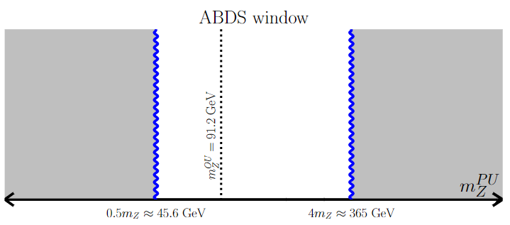
Figure 2: The ABDS-allowed window within the range of $m_{Z}^{PU}$ values.

While the exact upper bound on $m_{Z}^{PU}$ is not certain, what is important is that there is some distinct upper bound: for too large of values of $m_{Z}^{PU}$, then complex stable nuclei will not form, and hence the complex chemistry of our own universe will also not form. The explicit ABDS upper bound is quite distinct from many previous approaches which would penalize too large values of $m_{Z}^{PU}$ by a factor $(m_{weak}^{OU}/m_{SUSY})^{2}$, a putative finetuning factor which penalizes but does not disallow a large mass gap (a Little Hierarchy) between the SUSY breaking scale and the measured value of the weak scale.

Using conventional SUSY spectra generators where $m_{Z}$ is fixed to its measured value, then one may estimate the value of $m_{Z}^{PU}$ from the finetuning measure $\Delta_{EW}$ in the limit of no finetuning (where the weak scale is determined by the maximal value on the RHS of Eq. 4) as

$$m_{Z}^{PU}\simeq\sqrt{\Delta_{EW}/2}m_{Z}^{OU}$$ (8)

which gives for $\Delta_{EW}\sim 30$ a value $m_{Z}^{PU}\sim 360$ GeV, about four times its value $m_{Z}^{OU}$. We can then plot out the allowed range of MSSM weak scale parameters from Eq. 4 while setting the radiative corrections $\Sigma_{u}^{u}$ and $\Sigma_{d}^{d}$ to zero. The result is shown in Fig. 3 where we plot allowed values of $\mu^{PU}$ vs. $\sqrt{-m_{H_{u}}^{2}(weak)}$. To fulfill the requirement that $m_{Z}^{PU}\lesssim 4m_{Z}^{OU}$, then one must live in between the red and green curves. For parameter choices above the red curve then one obtains $m_{Z}^{PU}\gg m_{Z}^{OU}$ and the pocket universe value of the weak scale is too big. For points below the green curve, then $m_{Z}^{PU2}$ goes negative signalling inappropriate EWSB.

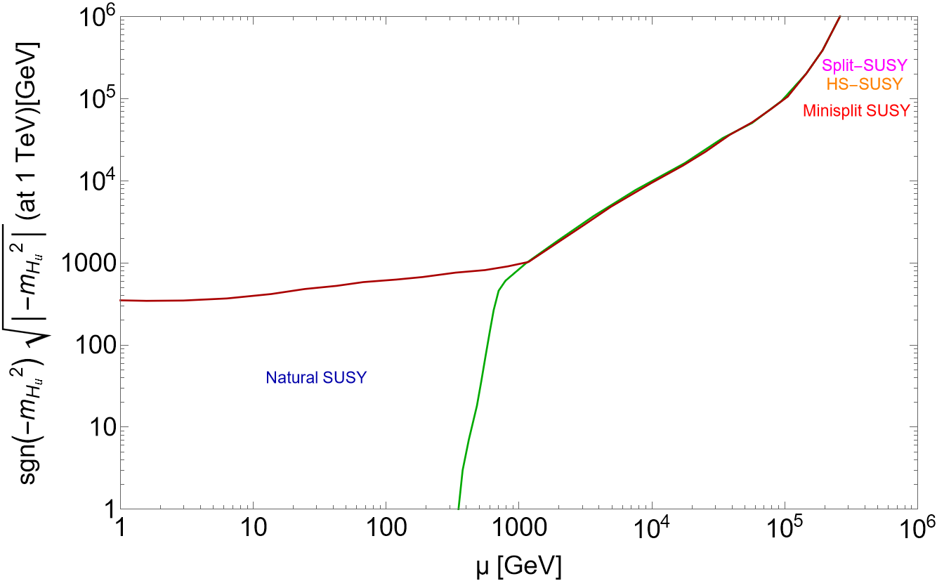
Figure 3: The $\mu^{PU}$ vs. $\sqrt{-m_{H_{u}}^{2}(weak)}$ parameter space in a toy model ignoring radiative corrections to the Higgs potential. The region between red and green curves leads to $m_{weak}^{PU}<4m_{weak}^{OU}$ so that the atomic principle is satisfied.

One immediately notices that there is a large range of parameter values in the lower-left corner of the plot that land in the ABDS window. Alternatively, for large values of $\mu^{PU}\gtrsim 360$ GeV and $\sqrt{-m_{H_{u}}^{2}(weak)}\gtrsim 360$ GeV, then in order to gain $m_{Z}^{PU}$ in the ABDS window one must land within the tiny gap between the red and green curves. Unnatural or finetuned SUSY models (such as High-Scale SUSY[61, 36], Split SUSY[62, 63] and Minisplit SUSY[33, 34], labelled in upper right) thus must fall in the narrow gap whilst natural SUSY models characterized by low $\Delta_{EW}$ would lie in the substantial lower-left allowed region. If $\mu^{PU}$ and $\sqrt{-m_{H_{u}}^{2}(weak)}$ were fundamental parameters (as in pMSSM) that were distributed in a scale invariant fashion (uniform on a log scale), then it would be easy to see why natural SUSY is more likely to emerge than finetuned SUSY from the landscape: for a random distribution of parameters (on a log scale), one is more likely to land in the large lower-left region than in the narrow gap between the red and green curves in the upper right.

Of course, the value of $m_{H_{u}}^{2}(weak)$ is highly distorted from its high scale value due to RG running and the requirement of radiatively-induced EWSB (REWSB). However, the value of $\mu^{PU}$ roughly tracks the high scale value of $\mu$ since $\mu$ does not run that much between high and low scales. In addition, the $\Sigma_{u,d}^{u,d}$ terms are not zero and can often be the dominant contributions to the RHS of Eq. 4. Our goal in this paper is to explore these connections numerically via a toy simulation of the multiverse.

4.1 The hypercube of ABDS-allowed parameter values in the NUHM2 model

Before we turn to our toy multiverse simulation, let us illustrate the hypercube of ABDS-allowed parameters for the simple case of the NUHM2 model. While a multi-dimensional portrayal of the hypercube is not possible, here we show $1-d$ parameter portrayals for the case where all other parameters are fixed. Thus, we adopt a NUHM2 benchmark model with $m_{0}=5$ TeV, $m_{1/2}=1.2$ TeV, $A_{0}=-8$ TeV, $\mu=200$ GeV and $m_{A}=2$ TeV with $\tan\beta=10$. This model has $m_{h}=124.7$ GeV with $\Delta_{EW}=22$ from the Isasugra spectrum generator[25].

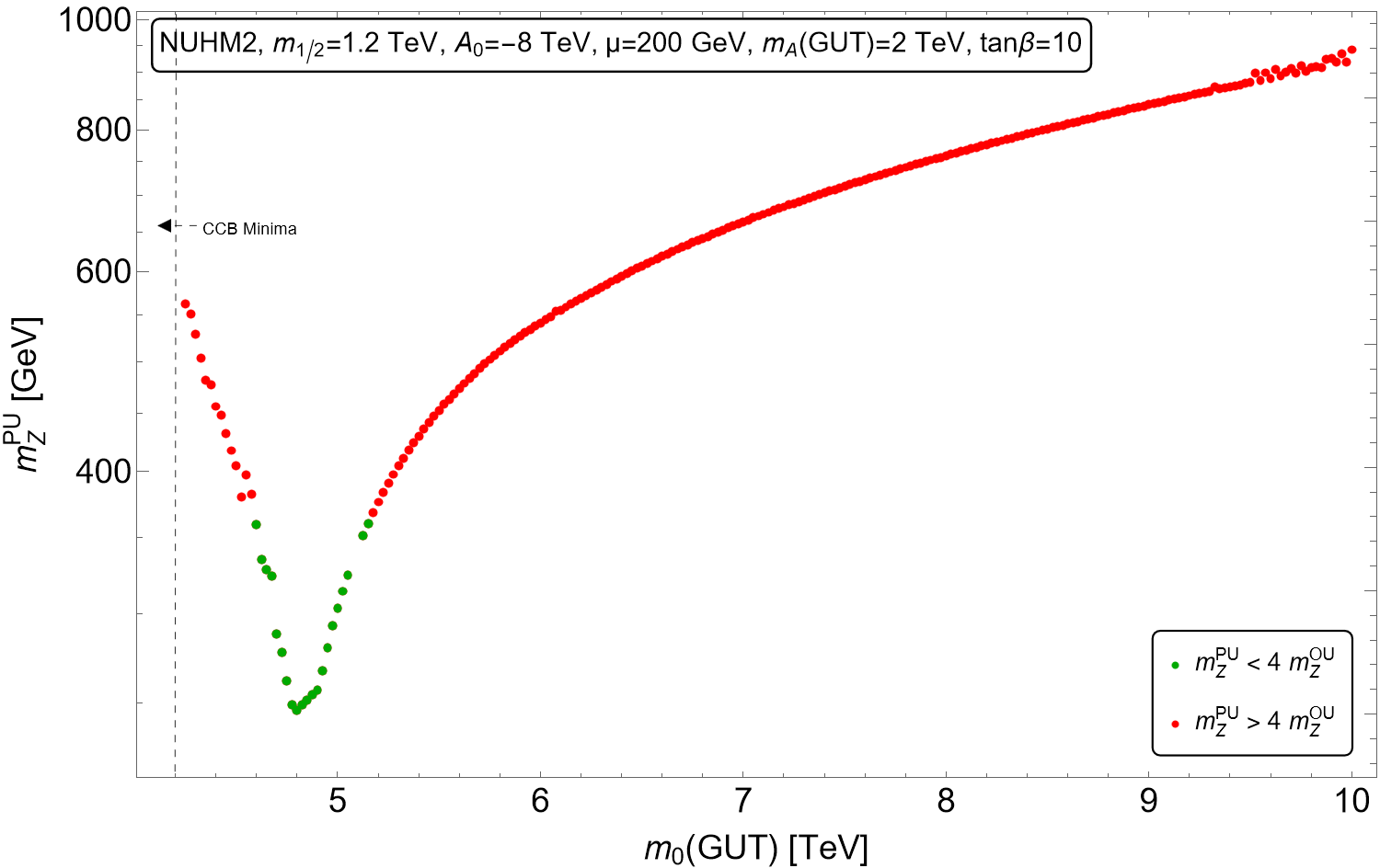
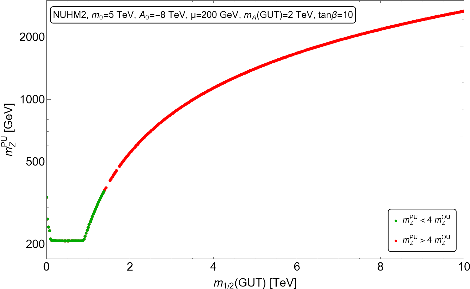
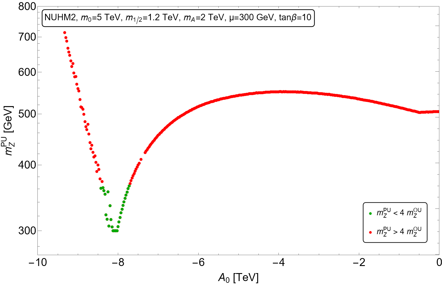
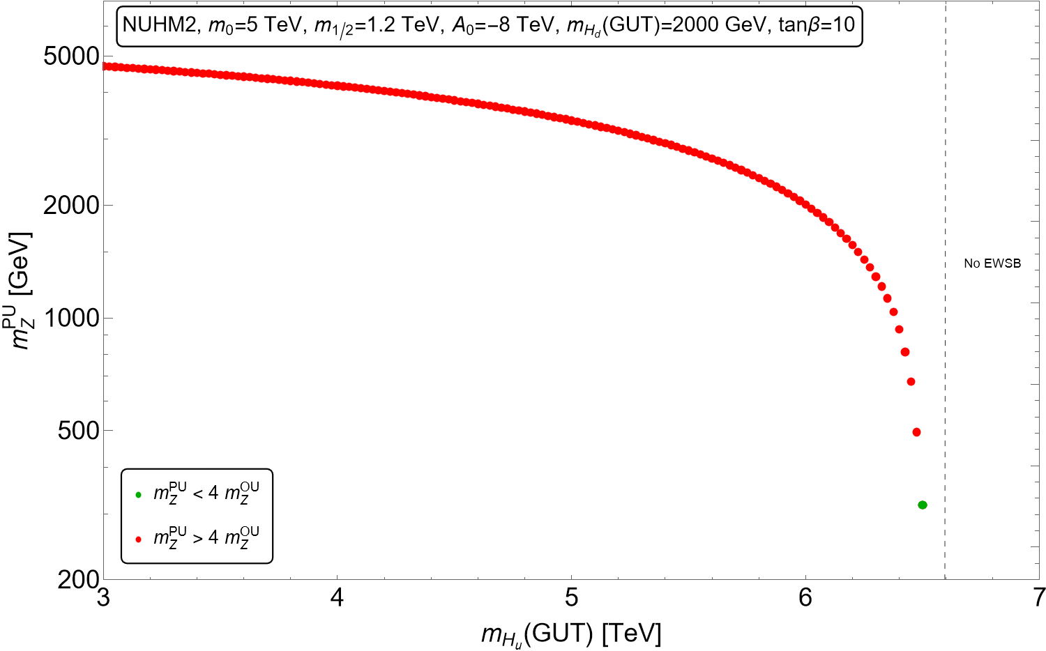
Figure 4: The value of $m_{weak}^{PU}$ vs. various NUHM2 model parameters to illustrate the substantial hypercube of parameter values which lead to $m_{Z}^{PU}$ within the ABDS window. The green points denote vacua with appropriate EWSB and with $m_{weak}^{PU}<4m_{weak}^{OU}$ so that the atomic principle is satisfied. Red points have $m_{weak}^{PU}>4m_{weak}^{OU}$. Parameter values include a) $m_{0}(1,2,3)$, b) $m_{1/2}$, c) $A_{0}$ and d) $m_{H_{u}}$.

In Fig. 4, we plot the value of $m_{Z}^{PU}$ versus variation in several soft SUSY breaking terms for a NUHM2 benchmark model. We take $m_{Z}^{PU}=\sqrt{\Delta_{EW}/2}m_{Z}^{OU}$. In frame a), we vary the parameter $m_{0}$. The red dots correspond to $m_{Z}^{PU}>4m_{Z}^{OU}$ while green points have $m_{Z}^{PU}<4m_{Z}^{OU}$. From the plot, we see range of $m_{0}:4.5-5.2$ TeV which leads to ABDS-allowed pocket universes. For larger or smaller values, then the $\Sigma_{u}^{u}(\tilde{t}_{1,2})$ values which enter Eq. 4 become too large and then finetuning is required to lie within the ABDS window. This range of allowed $m_{0}$ values is correlated with the window of $A_{0}$ values in that large cancellations can occur in both $\Sigma_{u}^{u}(\tilde{t}_{1})$ and $\Sigma_{u}^{u}(\tilde{t}_{2})$ for large $A_{0}$ at nearly maximal stop mixing which is where $m_{h}$ is lifted to $\sim 125$ GeV[29]. For lower or higher $m_{0}$ values, this cancellation is destroyed and top-squark loop contributions to the weak scale become too large.

In frame b), we show $m_{Z}^{PU}$ vs. variation in unified gaugino mass $m_{1/2}$. For very low $m_{1/2}$, then the $\mu$ term gives the dominant contribution to $m_{Z}^{PU}$. But as $m_{1/2}$ increases, then the top-squark contributions $\Sigma_{u}^{u}(\tilde{t}_{1,2})$ become large. Requiring $m_{Z}^{PU}\lesssim 4m_{Z}^{OU}$ places an upper bound on $m_{1/2}$, in this case around $1.5$ TeV. Thus, the window in $m_{1/2}$ lies between $0-1.5$ TeV.

In frame c), we show variation in $m_{Z}^{PU}$ vs. $-A_{0}$ (the negative values give cancellations in $\Sigma_{u}^{u}$ around the same values of $A_{0}$ which lift $m_{h}\sim 125$ GeV). Here we see the ABDS-allowed window extends from $\sim-7.5$ TeV to $\sim-8.5$ TeV; for this range, the $\Sigma_{u}^{u}(\tilde{t}_{1,2})$ contributions to $m_{Z}^{PU}$ are suppressed by cancellations.

Finally, in frame d), we show variation of $m_{Z}^{PU}$ vs. variation in $m_{H_{u}}$. In this case, for too small of values of $m_{H_{u}}(GUT)$, then the value of $m_{H_{u}}^{2}(weak)$ is driven to large negative values (see e.g. Fig. 4 of Ref. [12]), and hence gives a large contribution to $m_{Z}^{PU}$ via Eq. 4. As $m_{H_{u}}(GUT)$ increases, then $-m_{H_{u}}^{2}(weak)$ decreases, until at $m_{H_{u}}(GUT)\sim 6.5$ TeV, then electroweak symmetry is no longer broken and we do not generate a weak scale. Such pocket universes must be vetoed since they lack massive SM fermions and gauge bosons. The landscape pull on $m_{H_{u}}$ is to large values such that electroweak symmetry (EWS) is barely broken. While this viable portion of the hypercube looks small, it must be remembered that there is a landscape pull to large values stopping just short of the no EWSB limit (dashed vertical line). We can view this differently in Fig. 5 where instead we plot $m_{H_{u}}(GUT)$ on the $y$-axis and $m_{H_{u}}(weak)$ on the $x$-axis. In this case, the more substantial allowed range of $m_{H_{u}}(weak)$ values required by Fig. 3 is apparent as the green region on the right side of the curve.

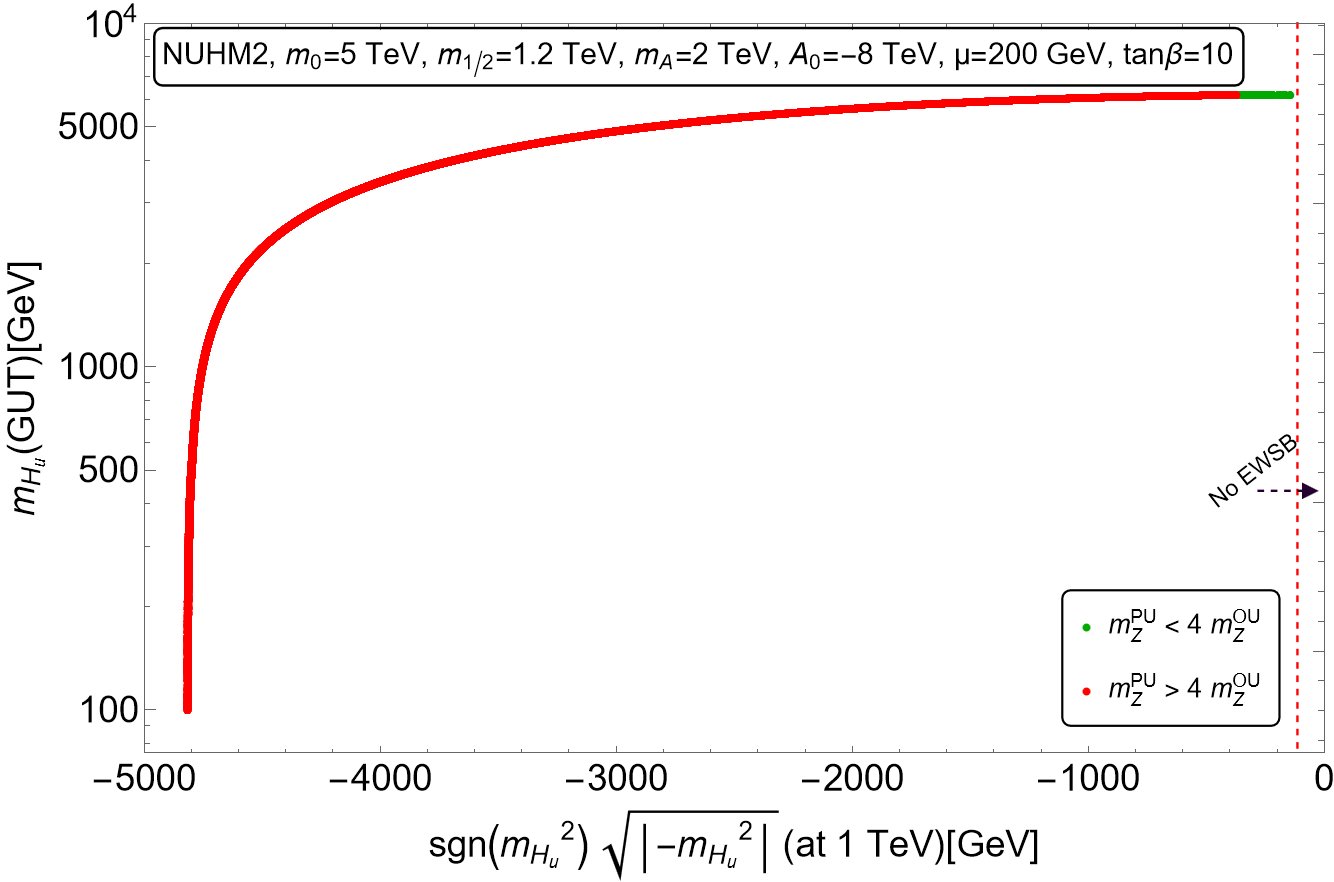
Figure 5: The value of $m_{H_{u}}(weak)\equiv sign(m_{H_{u}}^{2})\sqrt{-m_{H_{u}}^{2}(weak)}$ vs. $m_{H_{u}}(m_{GUT})$ The green points denote vacua with appropriate EWSB and with $m_{weak}^{PU}<4m_{weak}^{OU}$ so that the atomic principle is satisfied. Red points have $m_{weak}^{PU}>4m_{weak}^{OU}$.

5 A toy model of vacuum selection within the multiverse

Instead of using any of the publicly available SUSY spectra codes for which $m_{Z}$ is fixed at its measured value in our universe, we will construct a toy program with variable weak scale where both $\mu$ and $m_{H_{u}}$ are input parameters and $m_{Z}^{PU}\neq m_{Z}^{OU}$ is an output parameter. We begin by creating a code which solves the 26 coupled renormalization group equations (RGEs) of the MSSM via Runge-Kutta method starting with GUT scale inputs of parameters

$$m_{0}(1,2,3),\ m_{H_{u}},\ m_{H_{d}},\ m_{1/2},\ A_{0},\ \tan\beta,\ {\rm and}\ \mu$$ (9)

where we have used the EWSB minimization conditions to trade the bilinear soft term $b=B\mu$ for $\tan\beta$, but where we have not imposed the relation between $m_{H_{u}}(weak)$ and $\mu(weak)$ in terms of the measured value of $m_{Z}$. We use the one-loop RGEs but augmented by the two-loop terms from Eq. 11.22 of Ref. [64] which set the upper limits on first/second generation scalar masses. We run the set of soft terms, gauge and Yukawa couplings and $\mu$ term from $Q=m_{GUT}\simeq 2\times 10^{16}$ GeV down to the weak scale $Q_{weak}$ which we define as that scale at which $m_{H_{u}}^{2}$ first runs negative so long as $Q_{weak}<m_{0}(3)$. Otherwise, we set $Q_{weak}=m_{0}(3)$. This method implements the condition of barely broken EWSB[65]. Then, we use Eq. 4 to calculate $m_{Z}^{PU}$ to see if it lies within the ABDS window. We veto vacua with no EWSB or color-or-charge-breaking (CCB) minima (where charged or colored scalar squared masses run negative) as these would presumably lead to unlivable vacua.

In our toy simulation of this fertile patch (those vacua leading to the MSSM as the $4-d$ low energy EFT) of the string landscape, we will scan over parameters as such:

$$m_{0}(1,2) : 0-60\ {\rm TeV}$$ (10)

$$m_{0}(3) : 0.1-10\ {\rm TeV}$$ (11)

$$m_{H_{u}} : m_{0}(3)-2m_{0}(3)$$ (12)

$$m_{H_{d}}(\sim m_{A}) : 0.3-10\ {\rm TeV}$$ (13)

$$m_{1/2} : 0.5-3\ {\rm TeV}$$ (14)

$$-A_{0} : 0-50\ {\rm TeV}$$ (15)

$$\mu_{GUT} : 1-10^{4}\ {\rm TeV}$$ (16)

$$\tan\beta : 3-60$$ (17)

The soft terms are all scanned according to $f_{SUSY}\sim m_{soft}^{1}$ (as expected for SUSY breaking from a single $F$-term field) while $\mu$ is scanned according to $f_{\mu}\sim 1/\mu$. For $\tan\beta$, we scan uniformly.

6 Numerical results

6.1 Results for $m_{H_{u}}$ vs. $\mu$ plane

We are now ready to present results from our toy model simulation of vacuum selection from the multiverse, where for simplicity we restrict ourselves to those vacua with the MSSM as the low energy EFT, but where soft terms and the $\mu$ parameter vary from vacuum to vacuum, and with a linear draw to large soft terms (as expected in models with spontaneous supersymmetry breaking from a single $F$-term field where all field values are equally likely). In this case, since $\langle F\rangle$ is distributed randomly as a complex number, then the overall SUSY breaking scale $m_{SUSY}$ has a linear draw to large soft terms[18]. We couple this with the MSSM prediction for the magnitude of the weak scale as given by Eq. 4. This is one of the most important predictions of supersymmetric models. However, it is often hidden in phenomenological work since parameters are tuned in the computer codes so that the value of $m_{Z}$ has its numerical value as given in our universe.

In Fig. 6, we show the results of our toy model where $m_{Z}^{PU}\neq m_{Z}^{OU}$. We show results in the $\mu^{PU}$ vs. $sign(-m_{H_{u}}^{2})\sqrt{|-m_{H_{u}}^{2}|}(weak)$ parameter plane as in Fig. 3. We adopt parameter choices $m_{H_{u}}=1.3m_{0}$ and $A_{0}=-1.6m_{0}$ with $\tan\beta=10$ while allowing $m_{0}$ and $m_{1/2}$ to be statistically determined as in Sec. 5. The soft term $m_{H_{d}}$ is scanned over the range given above with $n=1$. The light blue points all have $m_{Z}^{PU}>4m_{Z}^{OU}$ and so lie beyond the ABDS window: the weak scale is too large to allow for formation of complex nuclei and hence atoms as we know them: these points are anthropically vetoed. The green points have values of $m_{Z}^{PU}<4m_{Z}^{OU}$ and hence fall within the ABDS window: these points should allow for formation of complex nuclei and obey the atomic principle[15]. We see that the bulk of allowed points live within the parameter hypercube as shown in Fig. 3. However, in our toy model, a small number of green points now do live beyond the Fig. 3 parameter hypercube. The latter points are generated with accidental finetuning of parameters such that $m_{Z}^{PU}$ is still less than $4m_{Z}^{OU}$ in spite of large contributions to the weak scale. Nonetheless, we do see that the natural SUSY models with $\mu^{PU}$ and $m_{H_{u}}(weak)\lesssim 360$ GeV are much more numerous than the finetuned solutions.

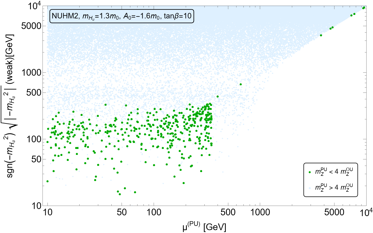
Figure 6: The value of $m_{H_{u}}(weak)$ vs. $\mu^{PU}$ The green points denote vacua with appropriate EWSB and with $m_{weak}^{PU}<4m_{weak}^{OU}$ so that the atomic principle is satisfied. Blue points have $m_{weak}^{PU}>4m_{weak}^{OU}$.

Let us compare the above results to the more common methodology of simply requiring $m_{Z}^{PU}=\sqrt{\Delta_{EW}/2}m_{Z}^{OU}<4m_{Z}^{OU}\simeq 360$ GeV (corresponding to $\Delta_{EW}<30$) as can be computed in available SUSY spectrum generators. We show these results as a scan in the same parameter space as in Fig. 3 but now as shown in Fig. 7. In this case, the weak scale is taken to be the largest of the elements contributing to the RHS of Eq. 4, so it assumes no finetuning of parameters within the landscape vacuum states. Again, the blue points lie beyond the ABDS window whilst the green points are anthropically allowed. In this case, the green points fill out the parameter hypercube of Fig. 3, albeit including the $\Sigma_{u,d}^{u,d}$ radiative corrections. Since no allowance for finetuning is made, then no green points extend along the finetuned diagonal in Fig. 7. The plot does show why the event generator runs with $f_{EWSB}=\Theta(30-\Delta_{EW})$ gives a good representation of expected superparticle and Higgs mass spectra in scans over the landscape of string vacua[19, 20, 17].

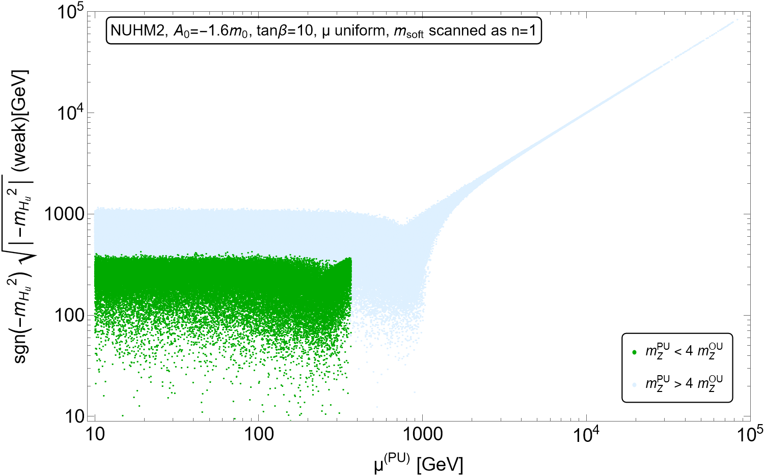
Figure 7: Points with $m_{Z}^{PU}<4m_{Z}^{OU}$ (green) from Isajet with $m_{Z}^{PU}<4m_{Z}^{OU}$ (green) and with $m_{Z}^{PU}>4m_{Z}^{OU}$ (blue) from the NUHM2 model. This run implements $m_{Z}^{PU}=\sqrt{\Delta_{EW}/2}m_{Z}^{OU}$.

6.2 Distribution of $\mu$ parameter

As a byproduct of our toy model of the string landscape, we are able to plot out the expected distribution of the superpotential $\mu$ parameter. This has also been done in Ref. [58] but in that case a fixed $\mu$-term Yukawa coupling $\lambda_{\mu}$ is adopted for a particularly well-motivated solution to the $\mu$ problem wherein the global $U(1)_{PQ}$ symmetry needed to solve the strong CP problem emerges as an accidental, approximate, gravity-safe global symmetry from a discrete anomaly-free $R$-symmetry ${\bf Z}_{24}^{R}$ which also solves the SUSY $\mu$ problem and provides a basis for $R$-parity[59]. In the present case, we allow $\lambda_{\mu}$ to also scan in the landscape so that $\mu$ is distributed uniformly across the decades of possible values, as may be expected for other superpotential terms (the matter Yukawa couplings) as shown by Donoghue et al.[60].

In Fig. 8, we show the distribution of the weak scale value of the SUSY $\mu$ parameter as expected from our toy landscape model where $\mu^{PU}$ is distributed as $P_{\mu}\sim 1/\mu$ and where we also require appropriate EWSB and $m_{Z}^{PU}<4m_{Z}^{OU}$. Other parameters are fixed as in Fig. 6. From the plot, we see that the $\mu^{PU}$ distribution is peaked at low values and falls off at higher $\mu^{PU}$ values of several hundred GeV, with a steep drop beyond the non-finetuned ABDS window which ends at $\mu\sim 360$ GeV. For our toy model, there is still some probability to gain $\mu^{PU}\gtrsim 360$ GeV due to the possibility of finetuning in our toy model. It should be noted that the lower range of $\mu$ values $\sim 100-200$ GeV is now under pressure from LHC soft dilepton plus jets plus MET searches[66, 67] via higgsino pair production[68, 69, 70, 71]. The plot also emphasizes that there would be a good chance that ILC would turn out to be a higgsino factory in addition to a Higgs factory for $\sqrt{s}\gtrsim 2m(higgsino)$[72, 73].

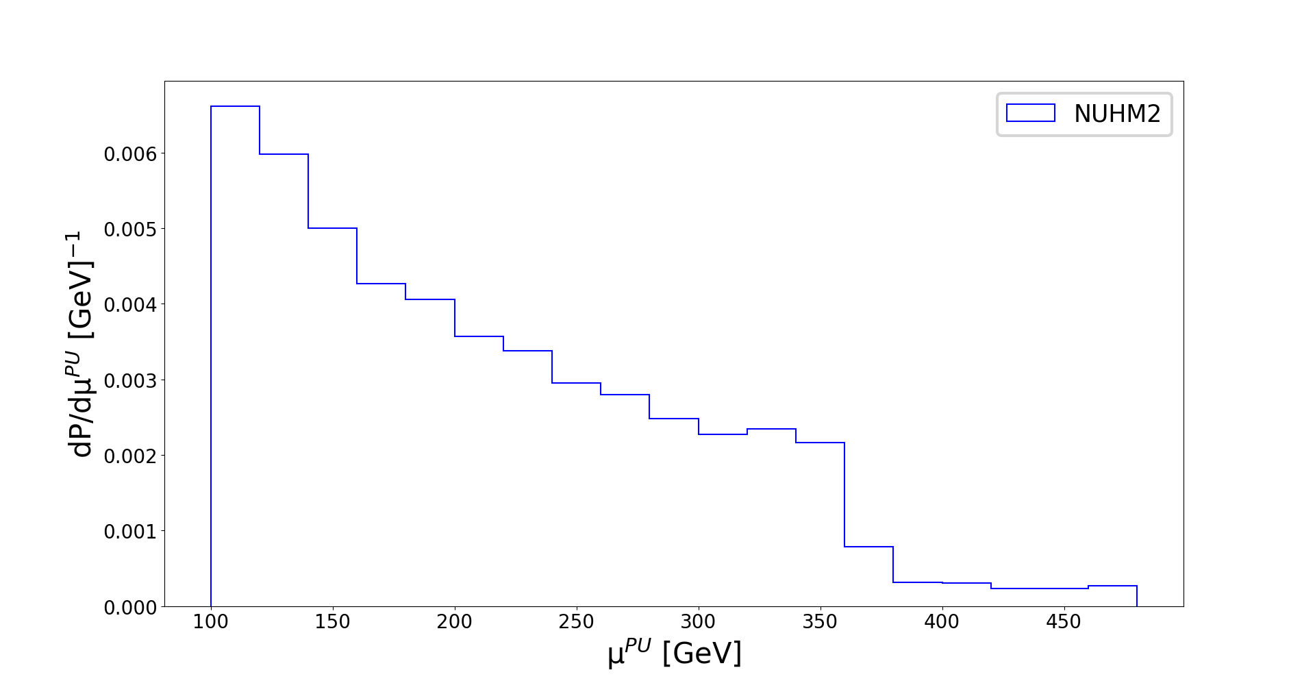
Figure 8: Distribution of $\mu$ parameter from scan over NUHM2 model with $P_{\mu}\sim 1/\mu$ and with $m_{Z}^{PU}<4m_{Z}^{OU}$ and with other parameters fixed as in Fig. 6.

6.3 Why finetuned SUSY models are scarce on the landscape compared to natural SUSY

In Fig. 6, we see that finetuned SUSY models that lie with parameters $\mu^{PU}$ and $m_{H_{u}}(weak)\gg 4m_{Z}^{OU}$ are relatively scarce in the multiverse compared to natural SUSY models with low $\Delta_{EW}$. While the finetuned models are logically possible, selection of their parameters is restricted to a hypercube of tiny-volume compared to natural SUSY models, and so we expect natural SUSY as the more likely expression of anthropically selected pocket universes.

We can show this in a different way in this subsection. In Fig. 9a), we adopt as an example our natural SUSY benchmark model as before, but with variable $\mu^{PU}$. We then plot the value of $m_{Z}^{PU}$ as obtained with our natural SUSY parameter choice but with varying $\mu^{PU}$. Recall, $\mu^{PU}$ is distributed uniformly across the decades of values using $f_{\mu}\sim 1/\mu^{PU}$. From frame a), we see a rather large window of $\mu^{PU}$ values from $100-210$ GeV which gives values of $m_{Z}^{PU}$ within the ABDS window (green portion of curve). For larger values of $\mu^{PU}$, $m_{Z}^{PU}$ drops below the ABDS window lower bound and then hits the boundary where electroweak symmetry is not properly broken.

In contrast, in Fig. 9b) we instead adopt a value of $m_{H_{u}}(GUT)<m_{0}$ so that $m_{H_{u}}^{2}$ is driven to large (unnatural) negative values at the weak scale. In this case, when we plot the $\mu^{PU}$ values needed to gain $m_{Z}^{PU}$ within the ABDS window, we find a tiny range of parameters around $\mu^{PU}\sim 4$ TeV which is anthropically allowed. Thus, compared to frame a), we see that, given a uniform distribution of $\mu$ parameter on the landscape, the unnatural model is logically possible– but highly improbable– compared to natural SUSY models.

Another example of a finetuned model occurring on the landscape comes from the CMSSM/mSUGRA model (frame c)) where all scalar masses are unified to $m_{0}$. In this case, with $m_{0}=5$ TeV, $m_{1/2}=1.2$ TeV, $A_{0}=0$ and $\tan\beta=10$ with $\mu>0$, one can see that a very thin range of $\mu^{PU}$ values around $2$ TeV allow for $m_{Z}^{PU}$ lying within the ABDS window. Thus, we would expect the CMSSM to also be rare on the landscape as compared to natural SUSY models which instead have non-universal scalar masses with $m_{H_{u}}(GUT)\sim 1.3m_{0}$ so that $m_{H_{u}}^{2}$ runs barley negative at the weak scale.

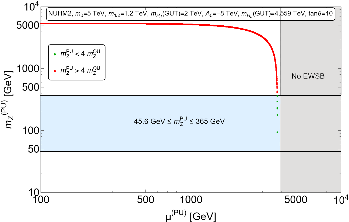
Figure 9: The value of $m_{weak}^{PU}$ vs. $\mu^{PU}$ The green points denote vacua with appropriate EWSB and with $m_{weak}^{PU}<4m_{weak}^{OU}$ so that the atomic principle is satisfied. Red points have $m_{weak}^{PU}>4m_{weak}^{OU}$.

7 Conclusions

Weak scale supersymmetry (WSS) provides a well-known solution to the gauge hierarchy problem of the Standard Model via cancellation of all quadratic divergences in scalar field masses. WSS is also suppported by a variety of virtual effects, especially gauge coupling unification and the numerical value of the Higgs boson mass. $N=1$ SUSY is expected as a byproduct of string theory compactified on a Calabi-Yau manifold. In models of string flux compactification, enormous numbers of vacuum states are possible which allows for Weinberg’s anthropic solution to the CC problem. The question then arises: what sort of soft terms arise statistically on the landscape, and what are the landscape predictions for WSS?

We addressed this question here via construction of a toy landscape model wherein the low energy EFT below the string scale was the MSSM but where each vacuum solution contained different soft term and $\mu$ term values. Under such conditions, it is expected there is a power-law draw to large soft terms favoring models with high scale SUSY breaking. However, since the soft terms and SUSY $\mu$ parameter determine the scale of EWSB, then anthropics provides an upper limit on the various soft terms: if they lead to too large a value of the pocket-universe weak scale, $m_{weak}^{PU}\gtrsim(2-5)m_{weak}^{OU}$ (the ABDS window), then complex nuclei and chemistry that seems necessary for life would not arise. This scenario has been used to motivate unnatural models like the SM valid to some high scale $Q\gg m_{weak}$, or other unnatural models of supersymmetry such as split, minisplit, PeV, spread SUSY or high scale SUSY.

Our toy simulation gives a counterexample in that models with low EW finetuning (radiatively-driven naturalness) have a comparatively large hypercube of parameter values on the landscape leading to a livable universe. For finetuned models, then the hypercube of anthropically-allowed parameters shrinks to a tiny volume relative to natural models. Thus, for a landscape populated with vacua including the MSSM as the low energy EFT, the unnatural models, while logically possible, are expected to be selected with much lower probability compared to natural SUSY models characterized by low $\Delta_{EW}$. This result is simply a byproduct of the finetuning needed for unnatural models which shrinks their hypercube of allowed parameter space to tiny volumes. As a result, we expect weak scale SUSY to ultimately emerge at sufficiently high energy colliders with $m_{h}\sim 125$ GeV but with sparticles typically beyond present LHC search limits. In the natural models, higgsinos must lie in the $100-350$ GeV range while top-squarks typically lie within the range $m_{\tilde{t}_{1}}\sim 1-2.5$ TeV with near maximal mixing (due to the landscape pull to large $A_{0}$ values) which easily distinguishes them from unnatural models which would have either far heavier top squarks or else top squarks with very low mixing.

Acknowledgements:

This material is based upon work supported by the U.S. Department of Energy, Office of Science, Office of High Energy Physics under Award Number DE-SC-0009956 and DE-SC-001764. Some of the computing for this project was performed at the OU Supercomputing Center for Education and Research (OSCER) at the University of Oklahoma (OU).

References

- [1] A. H. Guth, Inflation and eternal inflation, Phys. Rept. 333 (2000) 555–574. arXiv:astro-ph/0002156, doi:10.1016/S0370-1573(00)00037-5.
- [2] A. Linde, A brief history of the multiverse, Rept. Prog. Phys. 80 (2) (2017) 022001. arXiv:1512.01203, doi:10.1088/1361-6633/aa50e4.
- [3] S. Weinberg, Anthropic Bound on the Cosmological Constant, Phys. Rev. Lett. 59 (1987) 2607. doi:10.1103/PhysRevLett.59.2607.
- [4] H. Martel, P. R. Shapiro, S. Weinberg, Likely values of the cosmological constant, Astrophys. J. 492 (1998) 29. arXiv:astro-ph/9701099, doi:10.1086/305016.
- [5] R. Bousso, J. Polchinski, Quantization of four form fluxes and dynamical neutralization of the cosmological constant, JHEP 06 (2000) 006. arXiv:hep-th/0004134, doi:10.1088/1126-6708/2000/06/006.
- [6] M. R. Douglas, S. Kachru, Flux compactification, Rev. Mod. Phys. 79 (2007) 733–796. arXiv:hep-th/0610102, doi:10.1103/RevModPhys.79.733.
- [7] S. Ashok, M. R. Douglas, Counting flux vacua, JHEP 01 (2004) 060. arXiv:hep-th/0307049, doi:10.1088/1126-6708/2004/01/060.
- [8] W. Taylor, Y.-N. Wang, The F-theory geometry with most flux vacua, JHEP 12 (2015) 164. arXiv:1511.03209, doi:10.1007/JHEP12(2015)164.
- [9] V. Agrawal, S. M. Barr, J. F. Donoghue, D. Seckel, Viable range of the mass scale of the standard model, Phys. Rev. D 57 (1998) 5480–5492. arXiv:hep-ph/9707380, doi:10.1103/PhysRevD.57.5480.
- [10] V. Agrawal, S. M. Barr, J. F. Donoghue, D. Seckel, Anthropic considerations in multiple domain theories and the scale of electroweak symmetry breaking, Phys. Rev. Lett. 80 (1998) 1822–1825. arXiv:hep-ph/9801253, doi:10.1103/PhysRevLett.80.1822.
- [11] J. Elias-Miro, J. R. Espinosa, G. F. Giudice, G. Isidori, A. Riotto, A. Strumia, Higgs mass implications on the stability of the electroweak vacuum, Phys. Lett. B 709 (2012) 222–228. arXiv:1112.3022, doi:10.1016/j.physletb.2012.02.013.
- [12] H. Baer, V. Barger, S. Salam, Naturalness versus stringy naturalness (with implications for collider and dark matter searches), Phys. Rev. Research. 1 (2019) 023001. arXiv:1906.07741, doi:10.1103/PhysRevResearch.1.023001.
- [13] M. R. Douglas, Statistical analysis of the supersymmetry breaking scale (5 2004). arXiv:hep-th/0405279.
- [14] L. Susskind, Supersymmetry breaking in the anthropic landscape, in: From Fields to Strings: Circumnavigating Theoretical Physics: A Conference in Tribute to Ian Kogan, 2004, pp. 1745–1749. arXiv:hep-th/0405189, doi:10.1142/9789812775344_0040.
- [15] N. Arkani-Hamed, S. Dimopoulos, S. Kachru, Predictive landscapes and new physics at a TeV (1 2005). arXiv:hep-th/0501082.
- [16] I. Broeckel, M. Cicoli, A. Maharana, K. Singh, K. Sinha, Moduli Stabilisation and the Statistics of SUSY Breaking in the Landscape, JHEP 10 (2020) 015. arXiv:2007.04327, doi:10.1007/JHEP09(2021)019.
- [17] H. Baer, V. Barger, S. Salam, D. Sengupta, Landscape Higgs boson and sparticle mass predictions from a logarithmic soft term distribution, Phys. Rev. D 103 (3) (2021) 035031. arXiv:2011.04035, doi:10.1103/PhysRevD.103.035031.
- [18] H. Baer, V. Barger, M. Savoy, H. Serce, The Higgs mass and natural supersymmetric spectrum from the landscape, Phys. Lett. B 758 (2016) 113–117. arXiv:1602.07697, doi:10.1016/j.physletb.2016.05.010.
- [19] H. Baer, V. Barger, H. Serce, K. Sinha, Higgs and superparticle mass predictions from the landscape, JHEP 03 (2018) 002. arXiv:1712.01399, doi:10.1007/JHEP03(2018)002.
- [20] H. Baer, V. Barger, D. Sengupta, Mirage mediation from the landscape, Phys. Rev. Res. 2 (1) (2020) 013346. arXiv:1912.01672, doi:10.1103/PhysRevResearch.2.013346.
- [21] M. Dine, E. Gorbatov, S. D. Thomas, Low energy supersymmetry from the landscape, JHEP 08 (2008) 098. arXiv:hep-th/0407043, doi:10.1088/1126-6708/2008/08/098.
- [22] M. Dine, The Intermediate scale branch of the landscape, JHEP 01 (2006) 162. arXiv:hep-th/0505202, doi:10.1088/1126-6708/2006/01/162.
- [23] M. Dine, Supersymmetry, naturalness and the landscape, in: 10th International Symposium on Particles, Strings and Cosmology (PASCOS 04 and Pran Nath Fest), 2004, pp. 249–263. arXiv:hep-th/0410201, doi:10.1142/9789812701756_0093.
- [24] H. Baer, V. Barger, S. Salam, H. Serce, Supersymmetric particle and Higgs boson masses from the landscape: Dynamical versus spontaneous supersymmetry breaking, Phys. Rev. D 104 (11) (2021) 115025. arXiv:2103.12123, doi:10.1103/PhysRevD.104.115025.
- [25] F. E. Paige, S. D. Protopopescu, H. Baer, X. Tata, ISAJET 7.69: A Monte Carlo event generator for pp, anti-p p, and e+e- reactions (12 2003). arXiv:hep-ph/0312045.
- [26] H. Baer, V. Barger, D. Martinez, Comparison of SUSY spectra generators for natural SUSY and string landscape predictions (11 2021). arXiv:2111.03096.
- [27] H. Baer, V. Barger, P. Huang, D. Mickelson, A. Mustafayev, X. Tata, Radiative natural supersymmetry: Reconciling electroweak fine-tuning and the Higgs boson mass, Phys. Rev. D 87 (11) (2013) 115028. arXiv:1212.2655, doi:10.1103/PhysRevD.87.115028.
- [28] H. Baer, V. Barger, S. Salam, D. Sengupta, K. Sinha, Status of weak scale supersymmetry after LHC Run 2 and ton-scale noble liquid WIMP searches, Eur. Phys. J. ST 229 (21) (2020) 3085–3141. arXiv:2002.03013, doi:10.1140/epjst/e2020-000020-x.
- [29] H. Baer, V. Barger, P. Huang, A. Mustafayev, X. Tata, Radiative natural SUSY with a 125 GeV Higgs boson, Phys. Rev. Lett. 109 (2012) 161802. arXiv:1207.3343, doi:10.1103/PhysRevLett.109.161802.
- [30] H. Baer, V. Barger, D. Mickelson, How conventional measures overestimate electroweak fine-tuning in supersymmetric theory, Phys. Rev. D 88 (9) (2013) 095013. arXiv:1309.2984, doi:10.1103/PhysRevD.88.095013.
- [31] H. Baer, V. Barger, D. Mickelson, M. Padeffke-Kirkland, SUSY models under siege: LHC constraints and electroweak fine-tuning, Phys. Rev. D 89 (11) (2014) 115019. arXiv:1404.2277, doi:10.1103/PhysRevD.89.115019.
- [32] G. L. Kane, C. F. Kolda, L. Roszkowski, J. D. Wells, Study of constrained minimal supersymmetry, Phys. Rev. D 49 (1994) 6173–6210. arXiv:hep-ph/9312272, doi:10.1103/PhysRevD.49.6173.
- [33] A. Arvanitaki, N. Craig, S. Dimopoulos, G. Villadoro, Mini-Split, JHEP 02 (2013) 126. arXiv:1210.0555, doi:10.1007/JHEP02(2013)126.
- [34] N. Arkani-Hamed, A. Gupta, D. E. Kaplan, N. Weiner, T. Zorawski, Simply Unnatural Supersymmetry (12 2012). arXiv:1212.6971.
- [35] J. D. Wells, PeV-scale supersymmetry, Phys. Rev. D 71 (2005) 015013. arXiv:hep-ph/0411041, doi:10.1103/PhysRevD.71.015013.
- [36] G. F. Giudice, A. Strumia, Probing High-Scale and Split Supersymmetry with Higgs Mass Measurements, Nucl. Phys. B 858 (2012) 63–83. arXiv:1108.6077, doi:10.1016/j.nuclphysb.2012.01.001.
- [37] L. J. Hall, Y. Nomura, Spread Supersymmetry, JHEP 01 (2012) 082. arXiv:1111.4519, doi:10.1007/JHEP01(2012)082.
- [38] B. S. Acharya, K. Bobkov, G. L. Kane, J. Shao, P. Kumar, The G(2)-MSSM: An M Theory motivated model of Particle Physics, Phys. Rev. D 78 (2008) 065038. arXiv:0801.0478, doi:10.1103/PhysRevD.78.065038.
- [39] W. Buchmuller, K. Hamaguchi, O. Lebedev, M. Ratz, Local grand unification, in: GUSTAVOFEST: Symposium in Honor of Gustavo C. Branco: CP Violation and the Flavor Puzzle, 2005, pp. 143–156. arXiv:hep-ph/0512326.
- [40] F. Gabbiani, E. Gabrielli, A. Masiero, L. Silvestrini, A Complete analysis of FCNC and CP constraints in general SUSY extensions of the standard model, Nucl. Phys. B 477 (1996) 321–352. arXiv:hep-ph/9604387, doi:10.1016/0550-3213(96)00390-2.
- [41] H. Baer, V. Barger, M. Padeffke-Kirkland, X. Tata, Naturalness implies intra-generational degeneracy for decoupled squarks and sleptons, Phys. Rev. D 89 (3) (2014) 037701. arXiv:1311.4587, doi:10.1103/PhysRevD.89.037701.
- [42] N. Arkani-Hamed, H. Murayama, Can the supersymmetric flavor problem decouple?, Phys. Rev. D 56 (1997) R6733–R6737. arXiv:hep-ph/9703259, doi:10.1103/PhysRevD.56.R6733.
- [43] H. Baer, C. Balazs, P. Mercadante, X. Tata, Y. Wang, Viable supersymmetric models with an inverted scalar mass hierarchy at the GUT scale, Phys. Rev. D 63 (2001) 015011. arXiv:hep-ph/0008061, doi:10.1103/PhysRevD.63.015011.
- [44] H. Baer, V. Barger, D. Sengupta, Landscape solution to the SUSY flavor and CP problems, Phys. Rev. Res. 1 (3) (2019) 033179. arXiv:1910.00090, doi:10.1103/PhysRevResearch.1.033179.
- [45] H. P. Nilles, P. K. S. Vaudrevange, Geography of Fields in Extra Dimensions: String Theory Lessons for Particle Physics, Mod. Phys. Lett. A 30 (10) (2015) 1530008. arXiv:1403.1597, doi:10.1142/S0217732315300086.
- [46] F. Denef, M. R. Douglas, Distributions of nonsupersymmetric flux vacua, JHEP 03 (2005) 061. arXiv:hep-th/0411183, doi:10.1088/1126-6708/2005/03/061.
- [47] S. Kachru, R. Kallosh, A. D. Linde, S. P. Trivedi, De Sitter vacua in string theory, Phys. Rev. D 68 (2003) 046005. arXiv:hep-th/0301240, doi:10.1103/PhysRevD.68.046005.
- [48] S. Ferrara, L. Girardello, H. P. Nilles, Breakdown of Local Supersymmetry Through Gauge Fermion Condensates, Phys. Lett. B 125 (1983) 457. doi:10.1016/0370-2693(83)91325-4.
- [49] I. Affleck, M. Dine, N. Seiberg, Supersymmetry Breaking by Instantons, Phys. Rev. Lett. 51 (1983) 1026. doi:10.1103/PhysRevLett.51.1026.
- [50] V. Balasubramanian, P. Berglund, J. P. Conlon, F. Quevedo, Systematics of moduli stabilisation in Calabi-Yau flux compactifications, JHEP 03 (2005) 007. arXiv:hep-th/0502058, doi:10.1088/1126-6708/2005/03/007.
- [51] H. Baer, V. Barger, S. Salam, D. Sengupta, String landscape guide to soft SUSY breaking terms, Phys. Rev. D 102 (7) (2020) 075012. arXiv:2005.13577, doi:10.1103/PhysRevD.102.075012.
- [52] K. J. Bae, H. Baer, V. Barger, D. Sengupta, Revisiting the SUSY problem and its solutions in the LHC era, Phys. Rev. D 99 (11) (2019) 115027. arXiv:1902.10748, doi:10.1103/PhysRevD.99.115027.
- [53] G. F. Giudice, A. Masiero, A Natural Solution to the mu Problem in Supergravity Theories, Phys. Lett. B 206 (1988) 480–484. doi:10.1016/0370-2693(88)91613-9.
- [54] U. Ellwanger, C. Hugonie, A. M. Teixeira, The Next-to-Minimal Supersymmetric Standard Model, Phys. Rept. 496 (2010) 1–77. arXiv:0910.1785, doi:10.1016/j.physrep.2010.07.001.
- [55] J. E. Kim, H. P. Nilles, The mu Problem and the Strong CP Problem, Phys. Lett. B 138 (1984) 150–154. doi:10.1016/0370-2693(84)91890-2.
- [56] J. Bagger, E. Poppitz, L. Randall, Destabilizing divergences in supergravity theories at two loops, Nucl. Phys. B 455 (1995) 59–82. arXiv:hep-ph/9505244, doi:10.1016/0550-3213(95)00463-3.
- [57] S. A. Abel, S. Sarkar, P. L. White, On the cosmological domain wall problem for the minimally extended supersymmetric standard model, Nucl. Phys. B 454 (1995) 663–684. arXiv:hep-ph/9506359, doi:10.1016/0550-3213(95)00483-9.
- [58] H. Baer, V. Barger, D. Sengupta, R. W. Deal, Distribution of supersymmetry parameter and Peccei-Quinn scale fa from the landscape, Phys. Rev. D 104 (1) (2021) 015037. arXiv:2104.03803, doi:10.1103/PhysRevD.104.015037.
- [59] H. Baer, V. Barger, D. Sengupta, Gravity safe, electroweak natural axionic solution to strong and SUSY problems, Phys. Lett. B 790 (2019) 58–63. arXiv:1810.03713, doi:10.1016/j.physletb.2019.01.007.
- [60] J. F. Donoghue, K. Dutta, A. Ross, Quark and lepton masses and mixing in the landscape, Phys. Rev. D 73 (2006) 113002. arXiv:hep-ph/0511219, doi:10.1103/PhysRevD.73.113002.
- [61] G. Elor, H.-S. Goh, L. J. Hall, P. Kumar, Y. Nomura, Environmentally Selected WIMP Dark Matter with High-Scale Supersymmetry Breaking, Phys. Rev. D 81 (2010) 095003. arXiv:0912.3942, doi:10.1103/PhysRevD.81.095003.
- [62] N. Arkani-Hamed, S. Dimopoulos, Supersymmetric unification without low energy supersymmetry and signatures for fine-tuning at the LHC, JHEP 06 (2005) 073. arXiv:hep-th/0405159, doi:10.1088/1126-6708/2005/06/073.
- [63] N. Arkani-Hamed, S. Dimopoulos, G. F. Giudice, A. Romanino, Aspects of split supersymmetry, Nucl. Phys. B 709 (2005) 3–46. arXiv:hep-ph/0409232, doi:10.1016/j.nuclphysb.2004.12.026.
- [64] H. Baer, X. Tata, Weak scale supersymmetry: From superfields to scattering events, Cambridge University Press, 2006.
- [65] G. F. Giudice, R. Rattazzi, Living Dangerously with Low-Energy Supersymmetry, Nucl. Phys. B 757 (2006) 19–46. arXiv:hep-ph/0606105, doi:10.1016/j.nuclphysb.2006.07.031.
- [66] G. Aad, et al., Searches for electroweak production of supersymmetric particles with compressed mass spectra in 13 TeV collisions with the ATLAS detector, Phys. Rev. D 101 (5) (2020) 052005. arXiv:1911.12606, doi:10.1103/PhysRevD.101.052005.
- [67] Search for physics beyond the standard model in final states with two or three soft leptons and missing transverse momentum in proton-proton collisions at 13 TeV (2021).
- [68] Z. Han, G. D. Kribs, A. Martin, A. Menon, Hunting quasidegenerate Higgsinos, Phys. Rev. D 89 (7) (2014) 075007. arXiv:1401.1235, doi:10.1103/PhysRevD.89.075007.
- [69] H. Baer, A. Mustafayev, X. Tata, Monojet plus soft dilepton signal from light higgsino pair production at LHC14, Phys. Rev. D 90 (11) (2014) 115007. arXiv:1409.7058, doi:10.1103/PhysRevD.90.115007.
- [70] H. Baer, V. Barger, S. Salam, D. Sengupta, X. Tata, The LHC higgsino discovery plane for present and future SUSY searches, Phys. Lett. B 810 (2020) 135777. arXiv:2007.09252, doi:10.1016/j.physletb.2020.135777.
- [71] H. Baer, V. Barger, D. Sengupta, X. Tata, New angular (and other) cuts to improve the higgsino signal at the LHC (9 2021). arXiv:2109.14030.
- [72] H. Baer, V. Barger, D. Mickelson, A. Mustafayev, X. Tata, Physics at a Higgsino Factory, JHEP 06 (2014) 172. arXiv:1404.7510, doi:10.1007/JHEP06(2014)172.
- [73] H. Baer, M. Berggren, K. Fujii, J. List, S.-L. Lehtinen, T. Tanabe, J. Yan, ILC as a natural SUSY discovery machine and precision microscope: From light Higgsinos to tests of unification, Phys. Rev. D 101 (9) (2020) 095026. arXiv:1912.06643, doi:10.1103/PhysRevD.101.095026.