Principal manifold flows

Edmond Cunningham
edmondcunnin@cs.umass.edu
&Adam Cobb
adam.cobb@sri.com
\ANDSusmit Jha
susmit.jha@sri.com
Abstract

Normalizing flows map an independent set of latent variables to their samples using a bijective transformation. Despite the exact correspondence between samples and latent variables, their high level relationship is not well understood. In this paper we characterize the geometric structure of flows using principal manifolds and understand the relationship between latent variables and samples using contours. We introduce a novel class of normalizing flows, called principal manifold flows (PF), whose contours are its principal manifolds, and a variant for injective flows (iPF) that is more efficient to train than regular injective flows. PFs can be constructed using any flow architecture, are trained with a regularized maximum likelihood objective and can perform density estimation on all of their principal manifolds. In our experiments we show that PFs and iPFs are able to learn the principal manifolds over a variety of datasets. Additionally, we show that PFs can perform density estimation on data that lie on a manifold with variable dimensionality, which is not possible with existing normalizing flows.

1 Introduction

A normalizing flow is a generative model that generates a probability distribution by transforming a simple base distribution into a target distribution using a bijective function (Rezende and Mohamed, 2015; Papamakarios et al., 2019). Despite the fact that flows can compute the log likelihood of their samples exactly and associate a point in the data space with a unique point in the latent space, they are still poorly understood as generative models. This poor understanding stems from the unidentifiablity of their latent space - the latent space of a flow can be transformed into another valid latent space using any one of an infinite number of volume preserving transformations (Hyvärinen and Pajunen, 1999). Furthermore, methods that are rooted in mutual information (Alemi et al., 2018a; Higgins et al., 2017; Chen et al., 2016) that are used to understand other kinds of generative models break down when applied to flows because there is a deterministic mapping between the latent and data space (Ardizzone et al., 2020). To understand the generative process of flows, we need two items. The first is a set of informative structural properties of a probability distribution and the second is knowledge of how changes to the latent variables affect corresponding samples. We discuss the former using the concept of principal manifolds and the latter using contours.

The principal manifolds of a probability distribution can be understood as manifolds that span directions of maximum change (Gorban et al., 2008a). We locally define them using principal components which are the orthogonal directions of maximum variance around a data point, the same way that the principal components used in PCA (Jolliffe, 2011) are the orthogonal directions of maximum variance of a Gaussian approximation of a dataset. Principal manifolds capture the geometric structure of a probability distribution and are also an excellent fit for normalizing flows because it is possible to compute the principal components of a flow due to the bijective mapping between the latent and data spaces (see Definition 1).

The relationship between changes to latent variables and the effect on the corresponding sample in the data space can be understood through the contours of a flow. The contours of a flow are manifolds that trace the path that a sample can take when only some latent variables are changed. An important relationship we investigate is how the probability density on the contours relates to the probability density under the full model. This insight gives us a novel way to reason about how flows assign density to its samples.

We introduce a class of normalizing flows called principal manifold flows (PFs) whose contours are its principal manifolds. We develop deep insights into the generative behavior of normalizing flows that help explain how flows assign density to data points. This directly leads to a novel test time algorithm for density estimation on manifolds that requires no assumptions about the underlying data dimensionality. Furthermore, we develop two new algorithms that tackle separate important problems. The first is a learning algorithm to train PFs using any flow architecture, even those that can be difficult to invert, at a comparable cost to standard maximum likelihood. The second is an algorithm to train injective PFs that optimize a regularized maximum likelihood objective without needing to optimize a computationally expensive term found in the injective change of variables formula (Gemici et al., 2016). In our experiments we demonstrate the capabilities of PFs by learning the principal manifolds of low dimensional data and high dimensional data that is embedded on a low dimensional manifold, and show that PFs can learn the density of data that lies on a variable dimensional manifold - a task not possible using existing flow based methods. To summarize, our contributions are as follows:

  1. 1.

    We introduce a novel class of flows called PFs whose contours are principal manifolds and propose an efficient learning algorithm.

  2. 2.

    To overcome the computational cost of computing the expensive Jacobian determinant for PFs, we introduce iPFs as an approach for extending PFs to higher dimensional problems.

  3. 3.

    We introduce the first flow based solution to learning densities on manifolds with varying dimensionality.
Refer to caption
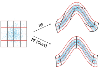
Figure 1: A principal manifold flow (PF) has contours that are its principal manifolds while standard normalizing flows do not. The blue dots represent samples from the prior and from each model, on the left and right plots respectively. The red and black lines represent the contours that emerge when a latent variable is held constant and the others vary. Movement in the latent space of a PF corresponds to movement along the principal manifolds (Theorem 1).

2 Preliminaries

2.1 Normalizing flows

Let f:𝒵=N𝒳=N:𝑓𝒵superscript𝑁𝒳superscript𝑁f:\mathcal{Z}=\mathbb{R}^{N}\to\mathcal{X}=\mathbb{R}^{N} be a parametric bijective function from a latent variable, 𝐳𝐳\mathbf{z}, to a data point 𝐱=f(𝐳)𝐱𝑓𝐳\mathbf{x}=f(\mathbf{z}) with inverse g(𝐱)=f1(𝐱)𝑔𝐱superscript𝑓1𝐱g(\mathbf{x})=f^{-1}(\mathbf{x}). The prior distribution over 𝐳𝐳\mathbf{z} will be denoted with p𝐳(𝐳)subscript𝑝𝐳𝐳p_{\mathbf{z}}(\mathbf{z}) and the Jacobian matrix of f𝑓f and g𝑔g will be denoted by J=df(𝐳)d𝐳𝐽𝑑𝑓𝐳𝑑𝐳J=\frac{df(\mathbf{z})}{d\mathbf{z}} and G=dg(𝐱)d𝐱𝐺𝑑𝑔𝐱𝑑𝐱G=\frac{dg(\mathbf{x})}{d\mathbf{x}}. The dependence of J𝐽J and G𝐺G on 𝐳𝐳\mathbf{z} or 𝐱𝐱\mathbf{x} is implied. A normalizing flow is a model that generates data by sampling 𝐳p𝐳(𝐳)similar-to𝐳subscript𝑝𝐳𝐳\mathbf{z}\sim p_{\mathbf{z}}(\mathbf{z}) and then computing 𝐱=f(𝐳)𝐱𝑓𝐳\mathbf{x}=f(\mathbf{z}) (Rezende and Mohamed, 2015; Papamakarios et al., 2019). The probability density of data points is computed using the change of variables formula:

logp𝐱(𝐱)=logp𝐳(g(𝐱))+log|G|subscript𝑝𝐱𝐱subscript𝑝𝐳𝑔𝐱𝐺\displaystyle\log p_{\mathbf{x}}(\mathbf{x})=\log p_{\mathbf{z}}(g(\mathbf{x}))+\log|G| (1)

Flows are typically comprised of a sequence of invertible functions f=f1fifK𝑓subscript𝑓1subscript𝑓𝑖subscript𝑓𝐾f=f_{1}\cdots f_{i}\cdots f_{K} where each fisubscript𝑓𝑖f_{i} has a Jacobian determinant that is easy to compute so that the overall Jacobian determinant, log|G|=i=1Klog|Gi|𝐺superscriptsubscript𝑖1𝐾subscript𝐺𝑖\log|G|=\sum_{i=1}^{K}\log|G_{i}| is also easy to compute. As a result, flows can be trained for maximum likelihood using an unbiased objective.

Eq. 1 can be generalized to the case where f𝑓f is an injective function that maps from a low dimensional 𝐳𝐳\mathbf{z} to a higher dimensional 𝐱𝐱\mathbf{x} (Gemici et al., 2016; Caterini et al., 2021). The change of variables formula in this case is written as:

logp𝐱(𝐱)=logp𝐳(𝐳)12log|JTJ|,𝐱=f(𝐳)formulae-sequencesubscript𝑝𝐱𝐱subscript𝑝𝐳𝐳12superscript𝐽𝑇𝐽𝐱𝑓𝐳\displaystyle\log p_{\mathbf{x}}(\mathbf{x})=\log p_{\mathbf{z}}(\mathbf{z})-\frac{1}{2}\log|J^{T}J|,\quad\mathbf{x}=f(\mathbf{z}) (2)

This general change of variables formula is valid over the manifold defined by f(𝒵)𝑓𝒵f(\mathcal{Z}). However, it is difficult to work with because the term log|JTJ|superscript𝐽𝑇𝐽\log|J^{T}J| cannot be easily decomposed into a sequence of simple Jacobian determinants as in the case where dim(𝐳)=dim(𝐱)dimension𝐳dimension𝐱\dim(\mathbf{z})=\dim(\mathbf{x}). In the remainder of this paper, logp𝐱(𝐱)subscript𝑝𝐱𝐱\log p_{\mathbf{x}}(\mathbf{x}) will refer to the definition given in Eq. 2 unless stated otherwise.

The requirement that f𝑓f is bijective is a curse and a blessing. The constraint prohibits flows from learning probability distributions with topology that does not match that of the prior (Cornish et al., 2019). This constraint limits a flow’s ability to learn the exact distribution of many real world datasets, including those that are thought to satisfy the manifold hypothesis (Fefferman et al., 2013). Nevertheless, invertibility makes it possible to compute the exact log likelihood under the model, associate any data point with a unique latent space vector, and affords access to geometric properties of the flow’s distribution (Dombrowski et al., 2021). In the remainder of this paper we focus on the latter - the geometric properties of a flow’s distribution through the use of principal manifolds and contours.

2.2 Principal components of a flow
Refer to caption
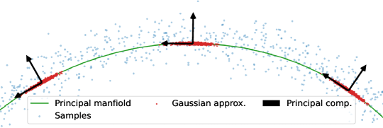
Figure 2: Illustration of principal components and a principal manifold of a flow. The blue dots are samples from a normalizing flow, red dots are samples from the Gaussian approximation defined in Definition 1, black arrows are the principal components and the green line is a principal manifold in Definition 2. Our main result in Theorem 1 states that the contours of principal manifold flows are its principal manifolds.

The structure of a probability distribution that is generated by a normalizing flow can be locally defined by examining how samples from the model are distributed around a data point.

Lemma 1.

Let 𝐱𝐱\mathbf{x} be a data point, f𝑓f be the invertible function of a flow and σ>0𝜎0\sigma>0 be a scalar. Consider samples that are generated by 𝐱=f(𝐳+σϵ)superscript𝐱𝑓𝐳𝜎italic-ϵ\mathbf{x}^{\prime}=f(\mathbf{z}+\sigma\mathbf{\epsilon}) where 𝐳=f1(𝐱)𝐳superscript𝑓1𝐱\mathbf{z}=f^{-1}(\mathbf{x}) and ϵN(0,I)similar-toitalic-ϵ𝑁0𝐼\mathbf{\epsilon}\sim N(0,I). Then 1σ(𝐱𝐱)𝐷N(0,JJT)1𝜎superscript𝐱𝐱𝐷𝑁0𝐽superscript𝐽𝑇\frac{1}{\sigma}(\mathbf{x}^{\prime}-\mathbf{x})\overset{D}{\to}N(0,JJ^{T}) as σ0𝜎0\sigma\to 0.

The lemma is true as a direct consequence of the Delta method (Oehlert, 1992). Lemma 1 says that points generated by a flow in a small region around a fixed point 𝐱𝐱\mathbf{x} will be approximately distributed as a Gaussian with mean 𝐱𝐱\mathbf{x} and covariance proportional to JJT𝐽superscript𝐽𝑇JJ^{T}. The principal components of data generated by a Gaussian distribution are the eigenvectors of the covariance matrix, so we can use the eigenvectors of JJT𝐽superscript𝐽𝑇JJ^{T} to define the principal components of a flow.

Definition 1 (Principal components of a flow at x𝑥x).

The principal components of a flow at 𝐱=f(𝐳)𝐱𝑓𝐳\mathbf{x}=f(\mathbf{z}) are the eigenvectors of JJT𝐽superscript𝐽𝑇JJ^{T}, 𝐰^^𝐰\hat{\mathbf{w}}, where J=df(𝐳)d𝐳𝐽𝑑𝑓𝐳𝑑𝐳J=\frac{df(\mathbf{z})}{d\mathbf{z}}. The principal components are ordered according to the eigenvalues of JJT𝐽superscript𝐽𝑇JJ^{T}.

The concept of principal components is shown in Fig. 2. Blue dots represent samples from a flow, red dots are samples from the local approximations drawn according to Lemma 1 and black arrows represent the principal components computed using Definition 1. We see that the red dots are approximately distributed as a Gaussian and the black arrows span their principal directions. Furthermore, the principal components are oriented along the main structure of the data. The global structure of a flow, which we call the "principal manifolds", are found by integrating along the principal components.

Definition 2 (Principal manifold of a flow).

The principal manifold of a flow is the path formed by integrating along principal components starting at 𝐱0subscript𝐱0\mathbf{x}_{0}. Let 𝕂𝕂\mathbb{K} be a subset of [1,,dim(𝐳)]1dimension𝐳[1,\dots,\dim(\mathbf{z})] and t|𝕂|𝑡superscript𝕂t\in\mathbb{R}^{|\mathbb{K}|}. A principal manifold of dimension |𝕂|𝕂|\mathbb{K}| is the solution to

d𝐱(t)dt=𝐰𝕂(𝐱(t)),𝐱(0)=𝐱0formulae-sequence𝑑𝐱𝑡𝑑𝑡subscript𝐰𝕂𝐱𝑡𝐱0subscript𝐱0\displaystyle\frac{d\mathbf{x}(t)}{dt}=\mathbf{w}_{\scriptscriptstyle\mathbb{K}}(\mathbf{x}(t)),\quad\mathbf{x}(0)=\mathbf{x}_{0} (3)

where 𝐰𝕂(𝐱(t))=𝐰^𝕂Λ𝕂subscript𝐰𝕂𝐱𝑡subscript^𝐰𝕂subscriptΛ𝕂\mathbf{w}_{\scriptscriptstyle\mathbb{K}}(\mathbf{x}(t))=\hat{\mathbf{w}}_{{\scriptscriptstyle\mathbb{K}}}\sqrt{\Lambda_{{\scriptscriptstyle\mathbb{K}}}} are the principal components with indices in 𝕂𝕂\mathbb{K} at 𝐱(t)𝐱𝑡\mathbf{x}(t) scaled by the square root of their corresponding eigenvalues.

The green curve in Fig. 2 is one of an infinite number of principal manifolds of the distribution. It spans the main structure of the samples and has principal component tangents. Principal manifolds can be used to reason about the geometric structure of a flow, but can only be found via integration over the principal components. Furthermore, there is no clear way compute the probability density over the principal manifolds. This is crucial when a principal manifold is used as a low dimensional representation of data and we still want to perform density estimation. We will revisit principal manifolds in Section 3.

2.3 Contours of a normalizing flow

The tool we use to analyze the generative properties of flows are the contours that emerge when some latent variables are held constant while others vary.

Definition 3 (Contours of a flow).

Let 𝕂𝕂\mathbb{K} be a subset of [1,,dim(𝐳)]1dimension𝐳[1,\dots,\dim(\mathbf{z})] and 𝐳𝕂subscript𝐳𝕂\mathbf{z}_{\scriptscriptstyle\mathbb{K}} be the latent variables with indices in 𝕂𝕂\mathbb{K}. Then, the contour obtained by varying 𝐳𝕂subscript𝐳𝕂\mathbf{z}_{\scriptscriptstyle\mathbb{K}} and fixing all other variables is denoted as f𝕂(𝐳𝕂)subscript𝑓𝕂subscript𝐳𝕂f_{\scriptscriptstyle\mathbb{K}}(\mathbf{z}_{\scriptscriptstyle\mathbb{K}}).

We assume that there is a partition over the indices of the latent space, 𝒫𝒫\mathcal{P}, so that every set of indices that we use to form contours is an element of the partition: 𝕂𝒫𝕂𝒫\mathbb{K}\in\mathcal{P}. Additionally, we assume that the prior over 𝐳𝐳\mathbf{z} can be factored into independent components in order to isolate a prior for each contour: p𝐳(𝐳)=𝕂𝒫p𝕂(𝐳𝕂)subscript𝑝𝐳𝐳subscriptproduct𝕂𝒫subscript𝑝𝕂subscript𝐳𝕂p_{\mathbf{z}}(\mathbf{z})=\prod_{\mathbb{K}\in\mathcal{P}}p_{\scriptscriptstyle\mathbb{K}}(\mathbf{z}_{\scriptscriptstyle\mathbb{K}}). This is not a limiting assumption as most flow architectures typically use a fully factorized prior such as a unit Gaussian prior (Papamakarios et al., 2019). The curved red and black lines in the right side plots of Fig. 1 are examples of contours. A red line on the left side plot is created by varying 𝐳1subscript𝐳1\mathbf{z}_{1} and fixing 𝐳2subscript𝐳2\mathbf{z}_{2} and becomes the contour f1(𝐳1)subscript𝑓1subscript𝐳1f_{1}(\mathbf{z}_{1}) after it is passed through the flow. Similarly, a black line on the left side plot is formed by varying 𝐳2subscript𝐳2\mathbf{z}_{2} and fixing 𝐳1subscript𝐳1\mathbf{z}_{1} and becomes the contour f2(𝐳2)subscript𝑓2subscript𝐳2f_{2}(\mathbf{z}_{2}) when it is transformed by the flow. The Jacobian matrix of f𝕂(𝐳𝕂)subscript𝑓𝕂subscript𝐳𝕂f_{\scriptscriptstyle\mathbb{K}}(\mathbf{z}_{\scriptscriptstyle\mathbb{K}}) is denoted by J𝕂subscript𝐽𝕂J_{\scriptscriptstyle\mathbb{K}} and is equal the matrix containing the columns of J𝐽J with indices in 𝕂𝕂\mathbb{K}. The log likelihood of a contour is denoted by 𝕂subscript𝕂\mathcal{L}_{\mathbb{K}} and is computed using the change of variables formula on manifolds in Eq. 2:

𝕂=Δlogp(f𝕂(𝐳𝕂))=logp𝕂(𝐳𝕂)12log|J𝕂TJ𝕂|subscript𝕂Δ𝑝subscript𝑓𝕂subscript𝐳𝕂subscript𝑝𝕂subscript𝐳𝕂12superscriptsubscript𝐽𝕂𝑇subscript𝐽𝕂\displaystyle\mathcal{L}_{\scriptscriptstyle\mathbb{K}}\overset{{\scriptstyle\Delta}}{=}\log p(f_{\scriptscriptstyle\mathbb{K}}(\mathbf{z}_{\scriptscriptstyle\mathbb{K}}))=\log p_{\mathbb{K}}(\mathbf{z}_{\scriptscriptstyle\mathbb{K}})-\frac{1}{2}\log|J_{\scriptscriptstyle\mathbb{K}}^{T}J_{\scriptscriptstyle\mathbb{K}}| (4)

A single flow can assign many different log likelihoods to a given data point that are not given by Eq. 1. Each of the |𝒫|𝒫|\mathcal{P}| contours that intersect at a data point can assign a density given by Eq. 4. Furthermore, the contours formed by grouping multiple 𝐳𝕂subscript𝐳𝕂\mathbf{z}_{\scriptscriptstyle\mathbb{K}} will assign other densities. In the next section we will relate all of these different densities.

2.4 Pointwise mutual information between contours

Consider two disjoint subsets of a latent variable, 𝐳𝕊subscript𝐳𝕊\mathbf{z}_{\scriptscriptstyle\mathbb{S}} and 𝐳𝕋subscript𝐳𝕋\mathbf{z}_{\scriptscriptstyle\mathbb{T}}, and their union 𝐳𝕊+𝕋subscript𝐳𝕊𝕋\mathbf{z}_{\scriptscriptstyle\mathbb{S+T}}. The densities of each contour can be related to the densities of their union using pointwise mutual information.

Definition 4 (Pointwise mutual information between disjoint contours).

Let 𝐳𝕊subscript𝐳𝕊\mathbf{z}_{\scriptscriptstyle\mathbb{S}} and 𝐳𝕋subscript𝐳𝕋\mathbf{z}_{\scriptscriptstyle\mathbb{T}} be disjoint subsets of z𝑧z. The pointwise mutual information between the contours for 𝐳𝕊subscript𝐳𝕊\mathbf{z}_{\scriptscriptstyle\mathbb{S}} and 𝐳𝕋subscript𝐳𝕋\mathbf{z}_{\scriptscriptstyle\mathbb{T}} is defined as

𝕊,𝕋subscript𝕊𝕋\displaystyle\mathcal{I}_{{\scriptscriptstyle\mathbb{S}},{\scriptscriptstyle\mathbb{T}}} =Δlogp(f𝕊+𝕋(𝐳𝕊+𝕋))p(f𝕊(𝐳𝕊))p(f𝕋(𝐳𝕋))=𝕊+𝕋𝕊𝕋Δ𝑝subscript𝑓𝕊𝕋subscript𝐳𝕊𝕋𝑝subscript𝑓𝕊subscript𝐳𝕊𝑝subscript𝑓𝕋subscript𝐳𝕋subscript𝕊𝕋subscript𝕊subscript𝕋\displaystyle\overset{{\scriptstyle\Delta}}{=}\log\frac{p(f_{\scriptscriptstyle\mathbb{S+T}}(\mathbf{z}_{\scriptscriptstyle\mathbb{S+T}}))}{p(f_{\scriptscriptstyle\mathbb{S}}(\mathbf{z}_{\scriptscriptstyle\mathbb{S}}))p(f_{\scriptscriptstyle\mathbb{T}}(\mathbf{z}_{\scriptscriptstyle\mathbb{T}}))}=\mathcal{L}_{\scriptscriptstyle\mathbb{S+T}}-\mathcal{L}_{\scriptscriptstyle\mathbb{S}}-\mathcal{L}_{\scriptscriptstyle\mathbb{T}} (5)

𝕊,𝕋subscript𝕊𝕋\mathcal{I}_{{\scriptscriptstyle\mathbb{S}},{\scriptscriptstyle\mathbb{T}}} plays an important role in describing the behavior of normalizing flows. We list a few important facts about 𝕊,𝕋subscript𝕊𝕋\mathcal{I}_{{\scriptscriptstyle\mathbb{S}},{\scriptscriptstyle\mathbb{T}}} below to help build intuition (more facts and proofs can be found in Appendix B):

Facts about 𝕊,𝕋subscript𝕊𝕋\mathcal{I}_{{\scriptscriptstyle\mathbb{S}},{\scriptscriptstyle\mathbb{T}}}
  1. 1.

    𝕊,𝕋0subscript𝕊𝕋0\mathcal{I}_{{\scriptscriptstyle\mathbb{S}},{\scriptscriptstyle\mathbb{T}}}\geq 0

  2. 2.

    𝕊,𝕋=0subscript𝕊𝕋0\mathcal{I}_{{\scriptscriptstyle\mathbb{S}},{\scriptscriptstyle\mathbb{T}}}=0 iff f𝕊(𝐳𝕊)subscript𝑓𝕊subscript𝐳𝕊f_{\scriptscriptstyle\mathbb{S}}(\mathbf{z}_{\scriptscriptstyle\mathbb{S}}) and f𝕋(𝐳𝕋)subscript𝑓𝕋subscript𝐳𝕋f_{\scriptscriptstyle\mathbb{T}}(\mathbf{z}_{\scriptscriptstyle\mathbb{T}}) intersect orthogonally.

  3. 3.

    𝕊,𝕋=12log|J𝕊+𝕋TJ𝕊+𝕋|+12log|J𝕊TJ𝕊|+12log|J𝕋TJ𝕋|subscript𝕊𝕋12superscriptsubscript𝐽𝕊𝕋𝑇subscript𝐽𝕊𝕋12superscriptsubscript𝐽𝕊𝑇subscript𝐽𝕊12superscriptsubscript𝐽𝕋𝑇subscript𝐽𝕋\mathcal{I}_{{\scriptscriptstyle\mathbb{S}},{\scriptscriptstyle\mathbb{T}}}=-\frac{1}{2}\log|J_{\scriptscriptstyle\mathbb{S+T}}^{T}J_{\scriptscriptstyle\mathbb{S+T}}|+\frac{1}{2}\log|J_{\scriptscriptstyle\mathbb{S}}^{T}J_{\scriptscriptstyle\mathbb{S}}|+\frac{1}{2}\log|J_{\scriptscriptstyle\mathbb{T}}^{T}J_{\scriptscriptstyle\mathbb{T}}|

𝕊,𝕋subscript𝕊𝕋\mathcal{I}_{{\scriptscriptstyle\mathbb{S}},{\scriptscriptstyle\mathbb{T}}} is a non-negative value that achieves its minimum of 00 when the contours intersect orthogonally. An equivalent condition is that the columns of J𝕊subscript𝐽𝕊J_{\scriptscriptstyle\mathbb{S}} and J𝕋subscript𝐽𝕋J_{\scriptscriptstyle\mathbb{T}} are mutually orthogonal. The third fact shows that 𝕊,𝕋subscript𝕊𝕋\mathcal{I}_{{\scriptscriptstyle\mathbb{S}},{\scriptscriptstyle\mathbb{T}}} has a closed form value that only depends on f𝑓f and not on the priors over 𝐳𝕊subscript𝐳𝕊\mathbf{z}_{\scriptscriptstyle\mathbb{S}} or 𝐳𝕋subscript𝐳𝕋\mathbf{z}_{\scriptscriptstyle\mathbb{T}}. Another way to think about 𝕊,𝕋subscript𝕊𝕋\mathcal{I}_{{\scriptscriptstyle\mathbb{S}},{\scriptscriptstyle\mathbb{T}}} is as the difference between the contour log likelihoods and that of their union:

𝕊+𝕋=𝕊+𝕋+𝕊,𝕋subscript𝕊𝕋subscript𝕊subscript𝕋subscript𝕊𝕋\displaystyle\mathcal{L}_{\scriptscriptstyle\mathbb{S+T}}=\mathcal{L}_{\scriptscriptstyle\mathbb{S}}+\mathcal{L}_{\scriptscriptstyle\mathbb{T}}+\mathcal{I}_{{\scriptscriptstyle\mathbb{S}},{\scriptscriptstyle\mathbb{T}}} (6)

If 𝕊+𝕋=[1,,dim(𝐳)]𝕊𝕋1dimension𝐳\mathbb{S}+\mathbb{T}=[1,\dots,\dim(\mathbf{z})], then we can decompose the change of variables formula into the sum of contour log likelihoods and 𝕊,𝕋subscript𝕊𝕋\mathcal{I}_{{\scriptscriptstyle\mathbb{S}},{\scriptscriptstyle\mathbb{T}}}. Next, we show that this decomposition can be extended to any partition of the latent space.

2.5 Change of variables formula decomposition
Refer to caption
(a) Example partitions of the latent space.
Refer to caption
(b) Decomposition of log likelihood.
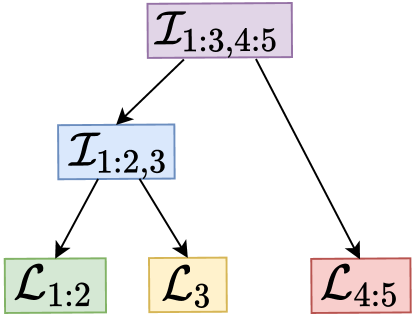
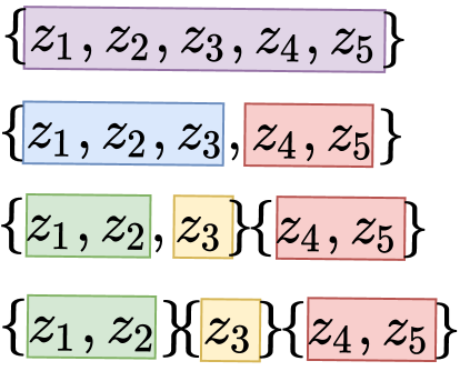
Figure 3: The general change of variables decomposition depends on the binary tree partition used to generate the latent space partition. Partitions are generated by recursively dividing existing partitions into two parts. The last row in Fig. 3(a) shows a partition of the latent space with 3 sets. Fig. 3(b) shows the corresponding log likelihood decomposition. Each parent node in the binary tree contributes an \mathcal{I} term and each leaf contributes a \mathcal{L} term. See Eq. 7 for the full formula.

Eq. 6 can be recursively applied to itself to yield a decomposition over any partition of the latent space. Consider a partition of the indices, 𝒫𝒫\mathcal{P}, like in Fig. 3(a). 𝒫𝒫\mathcal{P} can be constructed as the leaves of a binary tree, 𝒯𝒯\mathcal{T}, where each node is a subset of indices and each parent node is the union of its children. The corresponding decomposition in Fig. 3(b) is found by recursively applying Eq. 6 and tracking the leftover \mathcal{I} terms. This construction lets us decompose the change of variables formula into the sum of contours log likelihoods and pointwise mutual information terms:

logp𝐱(f(𝐳))=𝕂𝒫𝕂+parents(𝒯)L(),R()𝒫subscript𝑝𝐱𝑓𝐳subscript𝕂𝒫subscript𝕂subscriptsubscriptparents𝒯subscriptLRsubscript𝒫\displaystyle\log p_{\mathbf{x}}(f(\mathbf{z}))=\sum_{\mathbb{K}\in\mathcal{P}}\mathcal{L}_{\scriptscriptstyle\mathbb{K}}+\underbrace{\sum_{\mathbb{P}\in\text{parents}(\mathcal{T})}\mathcal{I}_{{\scriptscriptstyle\mathbb{\text{L}(P)}},{\scriptscriptstyle\mathbb{\text{R}(P)}}}}_{\mathcal{I}_{\mathcal{P}}} (7)

where L(p)L𝑝\text{L}({p}) and R(p)R𝑝\text{R}({p}) are the left and right children of \mathbb{P}, respectively. See Fig. 3 for a visual description. Notice that the sum of the various L(),R()subscriptLR\mathcal{I}_{{\scriptscriptstyle\mathbb{\text{L}(P)}},{\scriptscriptstyle\mathbb{\text{R}(P)}}} is independent of the choice of 𝒯𝒯\mathcal{T} because any 𝒯𝒯\mathcal{T} with the same leaves will have the same value of logp𝐱(f(𝐳))subscript𝑝𝐱𝑓𝐳\log p_{\mathbf{x}}(f(\mathbf{z})) and 𝕂𝒫𝕂subscript𝕂𝒫subscript𝕂\sum_{\mathbb{K}\in\mathcal{P}}\mathcal{L}_{\scriptscriptstyle\mathbb{K}}. This non-negative quantity is useful to know as it is the difference between the full log likelihood and sum of log likelihoods of the contours.

Definition 5 (Pointwise mutual information of a partition).

Let 𝒫𝒫\mathcal{P} be a partition of [1,,dim(𝐳)]1dimension𝐳[1,\dots,\dim(\mathbf{z})]. The pointwise mutual information of the flow whose latent space is partitioned by 𝒫𝒫\mathcal{P} is

𝒫subscript𝒫\displaystyle\mathcal{I}_{\mathcal{P}} =Δlogp𝐱(f(𝐳))𝕂𝒫𝕂Δsubscript𝑝𝐱𝑓𝐳subscript𝕂𝒫subscript𝕂\displaystyle\overset{{\scriptstyle\Delta}}{=}\log p_{\mathbf{x}}(f(\mathbf{z}))-\sum_{\mathbb{K}\in\mathcal{P}}\mathcal{L}_{\scriptscriptstyle\mathbb{K}} (8)

Eq. 7 gives insight into how normalizing flows assign density to data. The log likelihood of a data point under a normalizing flow is the sum of the log likelihoods under its contours, and a non-negative term that roughly measures the orthogonality of the contours. If during training Eq. 7 is maximized, as is the case in maximum likelihood learning, then 𝒫subscript𝒫\mathcal{I}_{\mathcal{P}} will surely not achieve its minimum value of 00. Therefore changes to different latent variables of a normalizing flow trained with maximum likelihood will likely produce similar changes in the data space.

2.6 Orthogonality condition using g

We have seen that 𝒫subscript𝒫\mathcal{I}_{\mathcal{P}} is a non-negative term that achieves it minimum of 00 when the contours of the flow are orthogonal. However obtaining its value requires computing columns of the Jacobian matrix of f(𝐳)𝑓𝐳f(\mathbf{z}). Many expressive normalizing flows layers (Huang et al., 2021; Chen et al., 2019; van den Berg et al., 2018) are constructed so that only g(𝐱)𝑔𝐱g(\mathbf{x}) is easy to evaluate while f(𝐳)𝑓𝐳f(\mathbf{z}) requires an expensive algorithm that can be difficult to differentiate. We introduce a novel alternate formulation of 𝕂subscript𝕂\mathcal{L}_{\scriptscriptstyle\mathbb{K}}, 𝕊,𝕋subscript𝕊𝕋\mathcal{I}_{{\scriptscriptstyle\mathbb{S}},{\scriptscriptstyle\mathbb{T}}} and 𝒫subscript𝒫\mathcal{I}_{\mathcal{P}} that can be computed with g(𝐱)𝑔𝐱g(\mathbf{x}) to mitigate this issue:

^𝕂subscript^𝕂\displaystyle\widehat{\mathcal{L}}_{\scriptscriptstyle\mathbb{K}} =Δlogp𝕂(𝐳𝕂)+12log|G𝕂G𝕂T|Δsubscript𝑝𝕂subscript𝐳𝕂12subscript𝐺𝕂superscriptsubscript𝐺𝕂𝑇\displaystyle\overset{{\scriptstyle\Delta}}{=}\log p_{\mathbb{K}}(\mathbf{z}_{\scriptscriptstyle\mathbb{K}})+\frac{1}{2}\log|G_{\scriptscriptstyle\mathbb{K}}G_{\scriptscriptstyle\mathbb{K}}^{T}| (9)
^𝕊,𝕋subscript^𝕊𝕋\displaystyle\widehat{\mathcal{I}}_{{\scriptscriptstyle\mathbb{S}},{\scriptscriptstyle\mathbb{T}}} =Δ^𝕊+𝕋^𝕊^𝕋Δsubscript^𝕊𝕋subscript^𝕊subscript^𝕋\displaystyle\overset{{\scriptstyle\Delta}}{=}\widehat{\mathcal{L}}_{\scriptscriptstyle\mathbb{S+T}}-\widehat{\mathcal{L}}_{\scriptscriptstyle\mathbb{S}}-\widehat{\mathcal{L}}_{\scriptscriptstyle\mathbb{T}} (10)
^𝒫subscript^𝒫\displaystyle\widehat{\mathcal{I}}_{\mathcal{P}} =Δlogp𝐱(𝐱)𝕂𝒫^𝕂Δsubscript𝑝𝐱𝐱subscript𝕂𝒫subscript^𝕂\displaystyle\overset{{\scriptstyle\Delta}}{=}\log p_{\mathbf{x}}(\mathbf{x})-\sum_{\mathbb{K}\in\mathcal{P}}\widehat{\mathcal{L}}_{\scriptscriptstyle\mathbb{K}} (11)

In contrast to 𝕊,𝕋subscript𝕊𝕋\mathcal{I}_{{\scriptscriptstyle\mathbb{S}},{\scriptscriptstyle\mathbb{T}}} and 𝒫subscript𝒫\mathcal{I}_{\mathcal{P}}, ^𝕊,𝕋subscript^𝕊𝕋\widehat{\mathcal{I}}_{{\scriptscriptstyle\mathbb{S}},{\scriptscriptstyle\mathbb{T}}} and ^𝒫subscript^𝒫\widehat{\mathcal{I}}_{\mathcal{P}} are both negative ^𝕊,𝕋,^𝒫0subscript^𝕊𝕋subscript^𝒫0\widehat{\mathcal{I}}_{{\scriptscriptstyle\mathbb{S}},{\scriptscriptstyle\mathbb{T}}},\widehat{\mathcal{I}}_{\mathcal{P}}\leq 0. See Appendix B for more properties. The most important of these properties is the following Lemma:

Lemma 2.

^𝒫=0subscript^𝒫0\widehat{\mathcal{I}}_{\mathcal{P}}=0 if and only if 𝒫=0subscript𝒫0\mathcal{I}_{\mathcal{P}}=0.

We will see that flows that satisfy 𝒫=0subscript𝒫0\mathcal{I}_{\mathcal{P}}=0 are of interest, so this lemma provides an equivalent condition that can be computed by any normalizing flow architecture.

3 Principal manifold flows

We now present our main contributions. We will first define PFs and discuss their theoretical properties then discuss learning algorithms to train PFs and injective PFs (iPF).

3.1 PF theory

Next, we formally define PFs and provide a theorem stating their primary feature (see Theorem 2 for the proof).

Definition 6 (principal manifold flow).

A principal manifold flow (PF) is a normalizing flow that satisfies 𝒫=0subscript𝒫0\mathcal{I}_{\mathcal{P}}=0 at all of its samples.

Theorem 1 (Contours of PFs).

The contours of a principal manifold flow are principal manifolds.

A compelling byproduct of Theorem 1 is that PFs can easily evaluate the probability density of their principal manifolds. As a result, PFs can perform density estimation on manifolds at test time without making any assumptions about the dimensionality of the data manifold. This is in stark contrast to existing flow based algorithms for density estimation on manifolds where the manifold dimensionality is fixed when the flow is created (Brehmer and Cranmer, 2020). In order to exploit this ability, we need a method to identify which contours correspond to which principal manifolds. Recall that the principal components are ordered according to the eigenvalues of JJT𝐽superscript𝐽𝑇JJ^{T}. Consider a PF where the partition size is 1. Then the diagonal elements of JTJsuperscript𝐽𝑇𝐽J^{T}J will be equal to the top dim(𝐳)dimension𝐳\dim(\mathbf{z}) eigenvalues of JJT𝐽superscript𝐽𝑇JJ^{T} because J𝐽J will be the product of a semi-orthogonal matrix and a diagonal matrix (see Item 7), so JTJsuperscript𝐽𝑇𝐽J^{T}J will be diagonal and its diagonal elements of JTJsuperscript𝐽𝑇𝐽J^{T}J can be used to identify which contour corresponds to which principal manifold. In the general case, JTJsuperscript𝐽𝑇𝐽J^{T}J is a block diagonal matrix so we can look at the square root of the determinant of each block matrix, |J𝕂TJ𝕂|12superscriptsuperscriptsubscript𝐽𝕂𝑇subscript𝐽𝕂12|J_{\scriptscriptstyle\mathbb{K}}^{T}J_{\scriptscriptstyle\mathbb{K}}|^{\frac{1}{2}}. |J𝕂TJ𝕂|12superscriptsuperscriptsubscript𝐽𝕂𝑇subscript𝐽𝕂12|J_{\scriptscriptstyle\mathbb{K}}^{T}J_{\scriptscriptstyle\mathbb{K}}|^{\frac{1}{2}} is how much the density around 𝐱𝐱\mathbf{x} is "stretched" along the contour f𝕂(𝐳𝕂)subscript𝑓𝕂subscript𝐳𝕂f_{\scriptscriptstyle\mathbb{K}}(\mathbf{z}_{\scriptscriptstyle\mathbb{K}}) to form the structure present in the data, so contours with small values of |J𝕂TJ𝕂|12superscriptsuperscriptsubscript𝐽𝕂𝑇subscript𝐽𝕂12|J_{\scriptscriptstyle\mathbb{K}}^{T}J_{\scriptscriptstyle\mathbb{K}}|^{\frac{1}{2}} correspond to a direction that contributes little to the overall structure.

This check can be used filter out components of log likelihood that are due to small variations such as noise incurred in the data collection process. For example, consider a PF trained on 2D data and at 𝐱𝐱\mathbf{x} we observe that log|J1TJ1|log|J2TJ2|much-greater-thansuperscriptsubscript𝐽1𝑇subscript𝐽1superscriptsubscript𝐽2𝑇subscript𝐽2\log|J_{1}^{T}J_{1}|\gg\log|J_{2}^{T}J_{2}|. Then the structure of the probability distribution at 𝐱𝐱\mathbf{x} should be primarily aligned with the contour f1(𝐳1)subscript𝑓1subscript𝐳1f_{1}(\mathbf{z}_{1}), so it might make sense to report the log likelihood of 𝐱𝐱\mathbf{x} on only this contour. We define this procedure below:

Definition 7 (Manifold corrected probability density).

Let 𝐱𝐱\mathbf{x} be a sample from a PF. The manifold corrected probability density of 𝐱𝐱\mathbf{x} is computed as

logp(𝐱)=𝕂𝒮𝕂,𝒮={𝕂:|J𝕂TJ𝕂|12>ϵ}formulae-sequencesubscript𝑝𝐱subscript𝕂𝒮subscript𝕂𝒮conditional-set𝕂superscriptsuperscriptsubscript𝐽𝕂𝑇subscript𝐽𝕂12italic-ϵ\displaystyle\log p_{\mathcal{M}}(\mathbf{x})=\sum_{\mathbb{K}\in\mathcal{S}}\mathcal{L}_{\scriptscriptstyle\mathbb{K}},\quad\mathcal{S}=\{\mathbb{K}:|J_{\scriptscriptstyle\mathbb{K}}^{T}J_{\scriptscriptstyle\mathbb{K}}|^{\frac{1}{2}}>\epsilon\} (12)

In experiment Section 5.2 we demonstrate an example where PFs correctly learns the density of data generated on a variable dimension manifold.

3.2 Learning algorithms

PF objective


The PF optimization problem is to minimize the negative log likelihood of data subject to the constraint that 𝒫=0subscript𝒫0\mathcal{I}_{\mathcal{P}}=0:

argminθ𝐱𝒟logp𝐱(𝐱;θ),s.t.𝒫(𝐱;θ)=0subscriptargmin𝜃subscript𝐱𝒟subscript𝑝𝐱𝐱𝜃s.t.subscript𝒫𝐱𝜃0\displaystyle\text{argmin}_{\theta}-\sum_{\mathbf{x}\in\mathcal{D}}\log p_{\mathbf{x}}(\mathbf{x};\theta),\quad\text{s.t.}\quad\mathcal{I}_{\mathcal{P}}(\mathbf{x};\theta)=0 (13)

We solve this problem with a regularized maximum likelihood objective:

L(θ)=𝐱𝒟logp𝐱(𝐱;θ)+α𝒫(𝐱;θ)L𝜃subscript𝐱𝒟subscript𝑝𝐱𝐱𝜃𝛼subscript𝒫𝐱𝜃\displaystyle\mathrm{L}(\theta)=\sum_{\mathbf{x}\in\mathcal{D}}-\log p_{\mathbf{x}}(\mathbf{x};\theta)+\alpha\mathcal{I}_{\mathcal{P}}(\mathbf{x};\theta)
=𝐳=g(𝐱),𝐱𝒟logp𝐳(𝐳)α12log|J(𝐳;θ)TJ(𝐳;θ)|absentsubscriptformulae-sequence𝐳𝑔𝐱𝐱𝒟subscript𝑝𝐳𝐳𝛼12𝐽superscript𝐳𝜃𝑇𝐽𝐳𝜃\displaystyle=\sum_{\mathbf{z}=g(\mathbf{x}),\mathbf{x}\in\mathcal{D}}-\log p_{\mathbf{z}}(\mathbf{z})-\frac{\alpha-1}{2}\log|J(\mathbf{z};\theta)^{T}J(\mathbf{z};\theta)|
+α2𝕂𝒫log|J𝕂(𝐳;θ)TJ𝕂(𝐳;θ)|𝛼2subscript𝕂𝒫subscript𝐽𝕂superscript𝐳𝜃𝑇subscript𝐽𝕂𝐳𝜃\displaystyle\quad\quad\quad\quad+\frac{\alpha}{2}\sum_{\mathbb{K}\in\mathcal{P}}\log|J_{\scriptscriptstyle\mathbb{K}}(\mathbf{z};\theta)^{T}J_{\scriptscriptstyle\mathbb{K}}(\mathbf{z};\theta)| (14)

where α𝛼\alpha is a hyperparameter. Note that in the special case where the partition 𝕂𝕂\mathbb{K} is 1 dimensional and dim(𝐱)=dim(𝐳)dimension𝐱dimension𝐳\dim(\mathbf{x})=\dim(\mathbf{z}), this is the objective function used in (Gresele et al., 2021). Although L(θ)L𝜃\mathrm{L}(\theta) is a valid objective, it requires that we compute g(𝐱)𝑔𝐱g(\mathbf{x}) and Jacobian-vector products with f(𝐳)𝑓𝐳f(\mathbf{z}), making it impractical for flows where only g(𝐱)𝑔𝐱g(\mathbf{x}) is easy to evaluate. We remedy this issue by replacing the constraint 𝒫=0subscript𝒫0\mathcal{I}_{\mathcal{P}}=0 with ^𝒫=0subscript^𝒫0\widehat{\mathcal{I}}_{\mathcal{P}}=0 as per Lemma 2. The result is a novel loss function for training flows to have orthogonal contours:

LPF(θ)=𝐱𝒟logp𝐱(𝐱;θ)α^𝒫(𝐱;θ)subscriptLPF𝜃subscript𝐱𝒟subscript𝑝𝐱𝐱𝜃𝛼subscript^𝒫𝐱𝜃\displaystyle\mathrm{L}_{\text{PF}}(\theta)=\sum_{\mathbf{x}\in\mathcal{D}}-\log p_{\mathbf{x}}(\mathbf{x};\theta)-\alpha\widehat{\mathcal{I}}_{\mathcal{P}}(\mathbf{x};\theta)
=𝐱𝒟logp𝐳(g(𝐱;θ))α+12log|G(𝐱;θ)G(𝐱;θ)T|absentsubscript𝐱𝒟subscript𝑝𝐳𝑔𝐱𝜃𝛼12𝐺𝐱𝜃𝐺superscript𝐱𝜃𝑇\displaystyle=\sum_{\mathbf{x}\in\mathcal{D}}-\log p_{\mathbf{z}}(g(\mathbf{x};\theta))-\frac{\alpha+1}{2}\log|G(\mathbf{x};\theta)G(\mathbf{x};\theta)^{T}|
+α2𝕂𝒫log|G𝕂(𝐱;θ)G𝕂(𝐱;θ)T|𝛼2subscript𝕂𝒫subscript𝐺𝕂𝐱𝜃subscript𝐺𝕂superscript𝐱𝜃𝑇\displaystyle\quad\quad\quad\quad+\frac{\alpha}{2}\sum_{\mathbb{K}\in\mathcal{P}}\log|G_{\scriptscriptstyle\mathbb{K}}(\mathbf{x};\theta)G_{\scriptscriptstyle\mathbb{K}}(\mathbf{x};\theta)^{T}| (15)

LPF(θ)subscriptLPF𝜃\mathrm{L}_{\text{PF}}(\theta) is the objective of choice when dim(x)=dim(z)dimension𝑥dimension𝑧\dim(x)=\dim(z). It provides a lightweight change to maximum likelihood training that can be applied to any flow architecture.

iPF objective


Next consider the case where dim(𝐱)>dim(𝐳)dimension𝐱dimension𝐳\dim(\mathbf{x})>\dim(\mathbf{z}). This appears in problems where we want to learn a low dimensional representation of data (Gemici et al., 2016; Brehmer and Cranmer, 2020; Caterini et al., 2021; Kumar et al., 2020). Although we can optimize L(θ)L𝜃\mathrm{L}(\theta) to learn a PF, naively optimizing Section 3.2 will require optimizing log|JTJ|superscript𝐽𝑇𝐽\log|J^{T}J|, which requires dim(𝐳)dimension𝐳\dim(\mathbf{z}) Jacobian-vector products or an iterative algorithm (Caterini et al., 2021). We avoid this problem by setting α=1𝛼1\alpha=1 in Section 3.2. This yields the iPF objective:

LiPF(θ)subscriptLiPF𝜃\displaystyle\mathrm{L}_{\text{iPF}}(\theta) =𝐱𝒟logp𝐱(𝐱;θ)+𝒫(𝐱;θ)absentsubscript𝐱𝒟subscript𝑝𝐱𝐱𝜃subscript𝒫𝐱𝜃\displaystyle=\sum_{\mathbf{x}\in\mathcal{D}}-\log p_{\mathbf{x}}(\mathbf{x};\theta)+\mathcal{I}_{\mathcal{P}}(\mathbf{x};\theta)
=𝐳=g(𝐱),𝐱𝒟logp𝐳(𝐳)+12𝕂𝒫log|J𝕂TJ𝕂|absentsubscriptformulae-sequence𝐳𝑔𝐱𝐱𝒟subscript𝑝𝐳𝐳12subscript𝕂𝒫superscriptsubscript𝐽𝕂𝑇subscript𝐽𝕂\displaystyle=\sum_{\mathbf{z}=g(\mathbf{x}),\mathbf{x}\in\mathcal{D}}-\log p_{\mathbf{z}}(\mathbf{z})+\frac{1}{2}\sum_{\mathbb{K}\in\mathcal{P}}\log|J_{\scriptscriptstyle\mathbb{K}}^{T}J_{\scriptscriptstyle\mathbb{K}}| (16)

The iPF objective is a novel lower bound on the log likelihood of a dataset that lies on a manifold. Clearly the bound is tight when 𝒫(𝐱;θ)=0subscript𝒫𝐱𝜃0\mathcal{I}_{\mathcal{P}}(\mathbf{x};\theta)=0, so the learned model must trade off how close its contours are to principal manifolds with how well it represents data - both of which are desirable properties to have in a generative model. The computational bottleneck of LiPF(θ)subscriptLiPF𝜃\mathrm{L}_{\text{iPF}}(\theta) is the log|J𝕂TJ𝕂|superscriptsubscript𝐽𝕂𝑇subscript𝐽𝕂\log|J_{\scriptscriptstyle\mathbb{K}}^{T}J_{\scriptscriptstyle\mathbb{K}}| terms, which each require |𝕂|𝕂|\mathbb{K}| Jacobian-vector products to compute. However, if |𝕂|dim(𝐳)much-less-than𝕂dimension𝐳|\mathbb{K}|\ll\dim(\mathbf{z}), then LiPF(θ)subscriptLiPF𝜃\mathrm{L}_{\text{iPF}}(\theta) is much more efficient to estimate than L(θ)L𝜃\mathrm{L}(\theta) (see the next paragraph on unbiased estimates). Section 3.2 on its own cannot be used for training because there are no guarantees that training data will satisfy the condition 𝐱=f(𝐳)𝐱𝑓𝐳\mathbf{x}=f(\mathbf{z}). Instead, we plug LiPF(θ)subscriptLiPF𝜃\mathrm{L}_{\text{iPF}}(\theta) into the algorithm described in section 4 of (Caterini et al., 2021). This algorithm projects training data onto the generative manifold and maximizes the likelihood of the projected data, while also minimizing the reconstruction error. See appendix Section D.3 for a full description.

Unbiased estimates of the objectives


In practice, we implement Section 3.2 and Section 3.2 by randomly selecting 𝕂𝒫𝕂𝒫\mathbb{K}\in\mathcal{P}, constructing |𝕂|𝕂|\mathbb{K}| one-hot vectors where each vector has a single 1 at an index in 𝕂𝕂\mathbb{K}, and evaluating each in a vector-Jacobian product (vjp) at g(𝐱)𝑔𝐱g(\mathbf{x}) or Jacobian-vector product (jvp) with f(𝐳)𝑓𝐳f(\mathbf{z}). If each 𝐳𝕂subscript𝐳𝕂\mathbf{z}_{\scriptscriptstyle\mathbb{K}} is 1 dimensional, then the PF objective only requires a single vjp or jvp. This means that the cost of training a PF is only slightly more expensive than training a regular normalizing flow and the cost of training an iPF is much more efficient than training an injective normalizing flow. We provide Python code in appendix Appendix A.
Refer to caption
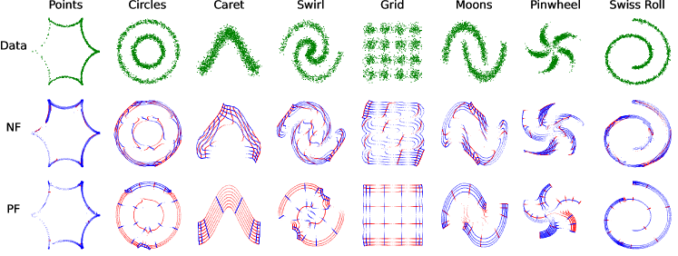
Figure 4: Contours for various synthetic datasets from a normalizing flow (NF) and principal manifold flow (PF). Both flows learned to produce the correct samples (see Section D.1) but only the PF learns the data’s structure.
Points Circles Caret Swirl Grid Moons Pinwheel Swiss Roll
logp(x)()𝑝𝑥\log p(x)(\mathbf{\uparrow}) NF -1.60 -3.10 -1.89 -0.19 -6.02 -0.64 -3.28 -4.67
PF -1.62 -3.12 -1.89 -0.20 -6.02 -0.66 -3.29 -4.68
𝒫()subscript𝒫\mathcal{I}_{\mathcal{P}}(\mathbf{\downarrow}) NF 1.60 1.18 0.61 0.71 0.39 0.64 0.77 1.38
PF 0.00 0.00 0.00 0.00 0.00 0.00 0.00 0.00
Table 1: Numerical results for learning synthetic datasets. The PF obtains a similar test set log likelihood to that of the normalizing flow (NF), but only the PF has small pointwise mutual information (𝒫subscript𝒫\mathcal{I}_{\mathcal{P}}). Small values of 𝒫subscript𝒫\mathcal{I}_{\mathcal{P}} result in the orthogonal contours shown in Fig. 4.

4 Related Work

Our work plugs a methodological gap in the normalizing flows (Papamakarios et al., 2019; Rezende and Mohamed, 2015) related to finding structure within flows. Although this is not crucial for applications such as density estimation or Neural-transport MCMC (Hoffman et al., 2019), the success of approaches in other deep generative models for finding low dimensional structure such as the β𝛽\beta-VAE (Higgins et al., 2017; Alemi et al., 2018b) and Style GAN (Karras et al., 2019) are motivation to find structure in normalizing flows. A subarea of flows research focuses on learning densities on manifolds. (Gemici et al., 2016) introduced a proof of concept for learning a density over a specified manifold and since then other methods have extended the idea to other kinds of manifolds such as toris, spheres and hyperbolic spaces (Rezende et al., 2020; Bose et al., 2020). A related class of flows are dedicated to both learning manifolds and densities over them (Kumar et al., 2020; Brehmer and Cranmer, 2020; Kalatzis et al., 2021; Caterini et al., 2021; Kothari et al., 2021). Our work is different because we focus on flows with density in the full data space and we do not focus on learning any single manifold. Additionally, there has been work in flows aimed at constructing architectures so that structure can emerge during training (Zhang et al., 2021; Cunningham et al., 2020; Cunningham and Fiterau, 2021), however these methods have no guarantees that they will recover the intended structure whereas PFs do.

There are other works that impose orthogonality conditions on Jacobian matrices. Conformal embedding flows (Ross and Cresswell, 2021) constructs an injective flow that has an orthogonal times a scalar Jacobian matrix to learn densities over manifolds. Our Jacobian structure is more flexible because it only requires JTJsuperscript𝐽𝑇𝐽J^{T}J to be block diagonal. We also note that our method can be used to learn conformal mappings if the regularizer is used on the Jacobian and its transpose. (Dombrowski et al., 2021) presents a way to apply flows that have learned the structure of a dataset to generating counterfactuals by using optimization in the latent space, which is shown to adhere to the flow’s generative manifold in the data space. Wei et al. (2021) and Gropp et al. (2020) propose regularizers to ensure that the Jacobian matrix of their models are orthogonal. As mentioned earlier, our Jacobian structure is much more flexible. The most similar work to ours is independent mechanism analysis (IMA) (Gresele et al., 2021). IMA is motivated by independent component analysis and causal inference while ours is motivated by uncovering the structure of data. We introduce novel insights on the geometry of flows and the densities on their contours, orthogonality conditions for both injective flows and flows that are not easily invertible, and a test time algorithm for computing densities on manifolds. PCA (Jolliffe, 2011) and its nonlinear extensions (Jolliffe, 2011; Gorban et al., 2008b) have the same goal as PFs of finding the principal structure of data. Cramer et al. (2021) treat PCA as a linear PF, but do not consider the nonlinear case. Work related to principal manifolds, such as locally linear embeddings (Ghojogh et al., 2021), differ from ours primarily in that we use parametric functions to learn the geometry of data.

5 Experiments
Refer to caption
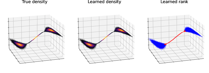
Figure 5: PFs are the only class of flows that can learn densities on manifolds with variable dimensionality. The dataset is generated on a manifold that is 1D near the origin and 2D elsewhere. At test time, the density for each data point is computed using Definition 7.

Our experiments showcase the capabilities of PFs to learn the principal manifolds of data, perform density estimation on data that is generated on a variable dimensional dataset, and learn high dimensional data embedded on a low dimensional manifold. All of our experiments were written using the JAX (Bradbury et al., 2018) Python library. We provide extended results and details of our models in Appendix D.

5.1 2D Synthetic Datasets

We trained standard normalizing flow and PF on various synthetic 2D datasets. Both flows have an architecture with 10 coupling layers, each with a logistic mixture cdf with 8 components, logit and shift-scale transformer (Ho et al., 2019; Papamakarios et al., 2019) and 5 layer residual network with 64 hidden units conditioner. We applied a matrix vector product and act norm layer in between each coupling layer (Kingma and Dhariwal, 2018). Note that logistic mixture cdfs require an iterative algorithm to invert.

The log likelihood and pointwise mutual information (𝒫)subscript𝒫(\mathcal{I}_{\mathcal{P}}) of the test sets are shown in Table 1. We see from the likelihoods that the PF is able to learn the datasets as well as the standard flow while achieving a small value of 𝒫subscript𝒫\mathcal{I}_{\mathcal{P}}. The low 𝒫subscript𝒫\mathcal{I}_{\mathcal{P}} is reflected by the contours in Fig. 4. In line with our theory, the contours of the PF are orthogonal to each other and are oriented in the directions of maximum variance.

5.2 Learning manifold densities of varying rank

PFs have the unique ability to learn densities on manifolds with unknown rank. All existing density estimation algorithms on manifolds using flows require specifying the dimensionality of the manifold beforehand, but PFs do not because they will automatically learn the underlying structure of the dataset. The leftmost plot of Fig. 5 shows the target probability distribution whose samples lie on either a 1D or 2D manifold. The data is generated by first sampling two univariate random variables z1subscript𝑧1z_{1} and z2subscript𝑧2z_{2} from a Gaussian mixture model and standard Gaussian respectively and then transforming z=(z1,z2)𝑧subscript𝑧1subscript𝑧2z=(z_{1},z_{2}) to the data space with the equation x=(z1,z2max(0,1|1z1|),sin(z1))𝑥subscript𝑧1subscript𝑧2max011subscript𝑧1subscript𝑧1x=(z_{1},z_{2}\text{max}(0,1-|\frac{1}{z_{1}}|),\sin(z_{1})). Notice that x𝑥x is one dimensional when |z1|<1subscript𝑧11|z_{1}|<1 and two dimensional otherwise. During training we perturb the dataset with a small amount of Gaussian noise so that the training data has full rank. See Section D.2 for a full description of the data and model and extended results. We use the method described in Definition 7 to compute the rank and density of each data point in the test set. We see from the center plot of Fig. 5 that the PF correctly recovers the densities of the test data samples. The final forward KL divergence from the learned density and true density is 0.0146.

5.3 iPF

Here we show that the iPF learning algorithm does in fact learn an injective flow with contours that are close to principal manifolds, and that the intuition about how contours relate to the principal manifolds does help explain the generative behavior of flows. We trained an iPF and standard injective normalizing flow (iNF) on the MNIST dataset (Lecun et al., 1998). The iPF and iNF both had the same architecture consisting of 20 layers of GLOW (Kingma and Dhariwal, 2018), a slice layer that removes all but 10 of the latent dimensions (so that the latent space is 10 dimensional), and then another 10 layers of neural spline flows (Durkan et al., 2019). See appendix Section D.3 for details on the model and the training. Note that the iPF required roughly 10 times less resources to train because we computed a single jvp to estimate Section 3.2 while the iNF required 10 jvps to compute Eq. 2.

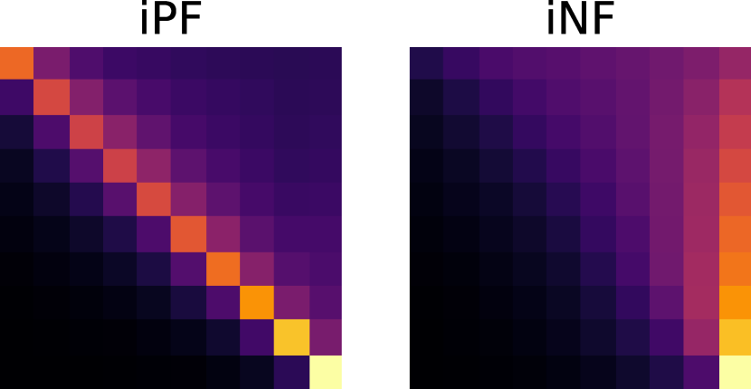
Fig. 6(a) shows a similarity plot between sorted contours of each model and the true principal components. The columns represent the principal components sorted by eigenvalue while the rows represent the tangents of the contours (columns of J𝐽J) in increasing order of the diagonal of JTJsuperscript𝐽𝑇𝐽J^{T}J. The intensity of each cell is the average absolute value of the cosine similarity between J𝐽J and a principal component. The plot of iPF is highlighted along the diagonal, which indicates that the contours are mostly aligned with the principal components whereas the plot for the iNF is highlighted along the last column, which indicates that the contours are mostly aligned with only the largest principal component.

Fig. 6(b) and Fig. 6(c) show a traversal of the largest and 5th largest contours of the iPF and iNF respectively. We moved along the contours by computing the Jacobian matrix of the flow at the current 𝐳𝐳\mathbf{z}, ordering the contours according to the diagonal of JTJsuperscript𝐽𝑇𝐽J^{T}J, and then taking a step of 0.020.020.02 on the dimension of 𝐳𝐳\mathbf{z} corresponding to the contour we want to traverse. We took 500 of these steps and displayed every 50thsuperscript50th50^{\text{th}} image in the figures. The images generated on the top contours for both models are varied as expected. The images on the 5th largest contours of the iPF are only varied slightly, which matches the results from Fig. 6(a) that the 5th largest contours will be oriented similarly to the 5th largest principal manifold and should therefore result in only a minimal amount of change. The iNF, on the other hand, generates images on the 5th largest contour that are similar to those generated on the largest contour. This also matches the intuition from Fig. 6(a) that the contours of the iNF are mostly aligned with the largest principal manifold.
Refer to caption (a)    Refer to caption (b) Refer to caption (c)

Figure 6: Similarity plot (Fig. 6(a)) between sorted contours of each model and the true principal components and traversal of the largest (Fig. 6(b)) and 5th largest (Fig. 6(c)) contours of the iPF and iNF. See Section 5.3 for more details.

6 Conclusion

We introduced principal manifold flows, a type of normalizing flow whose latent variables generate its principal manifolds. We investigated the generative behavior of flows using principal manifolds and contours to understand how a flow assign probability density to its samples. This analysis helped us define PFs and develop an efficient general purpose learning algorithm. Furthermore, we found an objective function to train injective PFs that avoided the need to compute a difficult Jacobian determinant during training. We showed how to interpret the contours of PFs and proposed a simple test to match a contour with a principal manifold. This test was then shown to help perform density estimation on the true data manifold at test time. Our experiments demonstrated the PFs are effective tools for learning the principal manifolds of low dimensional data, or high dimensional data that is embedded on a low dimensional manifold, and that PFs are capable of performing density estimation on data that is generated on a variable dimensional manifold.

Acknowledgments

This material is based upon work supported by U.S. Army Research Laboratory Cooperative Research Agreement W911NF-17-2-0196, U.S. National Science Foundation(NSF) grants #1740079, and the United States Air Force and DARPA under Contract No. FA8750-20-C-0002. The views, opinions and/or findings expressed are those of the author(s) and should not be interpreted as representing the official views or policies of the Department of Defense or the U.S. Government.

References

  • Rezende and Mohamed (2015) Danilo Rezende and Shakir Mohamed. Variational inference with normalizing flows. In Francis Bach and David Blei, editors, Proceedings of the 32nd International Conference on Machine Learning, volume 37 of Proceedings of Machine Learning Research, pages 1530–1538, Lille, France, 07–09 Jul 2015. PMLR. URL http://proceedings.mlr.press/v37/rezende15.html.
  • Papamakarios et al. (2019) George Papamakarios, Eric Nalisnick, Danilo Jimenez Rezende, Shakir Mohamed, and Balaji Lakshminarayanan. Normalizing Flows for Probabilistic Modeling and Inference. arXiv:1912.02762 [cs, stat], December 2019. URL http://arxiv.org/abs/1912.02762. arXiv: 1912.02762.
  • Hyvärinen and Pajunen (1999) Aapo Hyvärinen and Petteri Pajunen. Nonlinear independent component analysis: Existence and uniqueness results. Neural Netw., 12(3):429–439, apr 1999. ISSN 0893-6080. doi: 10.1016/S0893-6080(98)00140-3. URL https://doi.org/10.1016/S0893-6080(98)00140-3.
  • Alemi et al. (2018a) Alexander Alemi, Ben Poole, Ian Fischer, Joshua Dillon, Rif A. Saurous, and Kevin Murphy. Fixing a Broken ELBO. In Jennifer Dy and Andreas Krause, editors, Proceedings of the 35th International Conference on Machine Learning, volume 80 of Proceedings of Machine Learning Research, pages 159–168. PMLR, July 2018a. URL https://proceedings.mlr.press/v80/alemi18a.html.
  • Higgins et al. (2017) Irina Higgins, Loic Matthey, Arka Pal, Christopher Burgess, Xavier Glorot, Matthew Botvinick, Shakir Mohamed, and Alexander Lerchner. beta-vae: Learning basic visual concepts with a constrained variational framework. 2017.
  • Chen et al. (2016) Xi Chen, Yan Duan, Rein Houthooft, John Schulman, Ilya Sutskever, and Pieter Abbeel. Infogan: Interpretable representation learning by information maximizing generative adversarial nets. In Proceedings of the 30th International Conference on Neural Information Processing Systems, pages 2180–2188, 2016.
  • Ardizzone et al. (2020) Lynton Ardizzone, Radek Mackowiak, Carsten Rother, and Ullrich Köthe. Training Normalizing Flows with the Information Bottleneck for Competitive Generative Classification. In H. Larochelle, M. Ranzato, R. Hadsell, M. F. Balcan, and H. Lin, editors, Advances in Neural Information Processing Systems, volume 33, pages 7828–7840. Curran Associates, Inc., 2020. URL https://proceedings.neurips.cc/paper/2020/file/593906af0d138e69f49d251d3e7cbed0-Paper.pdf.
  • Gorban et al. (2008a) Alexander N Gorban, Balázs Kégl, Donald C Wunsch, Andrei Y Zinovyev, et al. Principal manifolds for data visualization and dimension reduction, volume 58. Springer, 2008a.
  • Jolliffe (2011) Ian Jolliffe. Principal Component Analysis, pages 1094–1096. Springer Berlin Heidelberg, Berlin, Heidelberg, 2011. ISBN 978-3-642-04898-2. doi: 10.1007/978-3-642-04898-2_455. URL https://doi.org/10.1007/978-3-642-04898-2_455.
  • Gemici et al. (2016) Mevlana C. Gemici, Danilo Rezende, and Shakir Mohamed. Normalizing Flows on Riemannian Manifolds. arXiv:1611.02304 [cs, math, stat], November 2016. URL http://arxiv.org/abs/1611.02304. arXiv: 1611.02304.
  • Caterini et al. (2021) Anthony L. Caterini, Gabriel Loaiza-Ganem, Geoff Pleiss, and John Patrick Cunningham. Rectangular Flows for Manifold Learning. In ICML Workshop on Invertible Neural Networks, Normalizing Flows, and Explicit Likelihood Models, 2021. URL https://openreview.net/forum?id=s-Fg3dXQzyS.
  • Cornish et al. (2019) Rob Cornish, Anthony L. Caterini, George Deligiannidis, and Arnaud Doucet. Relaxing bijectivity constraints with continuously indexed normalising flows, 2019.
  • Fefferman et al. (2013) Charles Fefferman, Sanjoy Mitter, and Hariharan Narayanan. Testing the Manifold Hypothesis. arXiv:1310.0425 [math, stat], December 2013. URL http://arxiv.org/abs/1310.0425. arXiv: 1310.0425.
  • Dombrowski et al. (2021) Ann-Kathrin Dombrowski, Jan E Gerken, and Pan Kessel. Diffeomorphic explanations with normalizing flows. In ICML Workshop on Invertible Neural Networks, Normalizing Flows, and Explicit Likelihood Models, 2021. URL https://openreview.net/forum?id=ZBR9EpEl6G4.
  • Oehlert (1992) Gary W. Oehlert. A note on the delta method. The American Statistician, 46(1):27–29, 1992. doi: 10.1080/00031305.1992.10475842. URL https://www.tandfonline.com/doi/abs/10.1080/00031305.1992.10475842.
  • Huang et al. (2021) Chin-Wei Huang, Ricky T. Q. Chen, Christos Tsirigotis, and Aaron Courville. Convex Potential Flows: Universal Probability Distributions with Optimal Transport and Convex Optimization. In International Conference on Learning Representations, 2021. URL https://openreview.net/forum?id=te7PVH1sPxJ.
  • Chen et al. (2019) Ricky T. Q. Chen, Jens Behrmann, David K Duvenaud, and Joern-Henrik Jacobsen. Residual Flows for Invertible Generative Modeling. In H. Wallach, H. Larochelle, A. Beygelzimer, F. d\textquotesingle Alché-Buc, E. Fox, and R. Garnett, editors, Advances in Neural Information Processing Systems, volume 32. Curran Associates, Inc., 2019. URL https://proceedings.neurips.cc/paper/2019/file/5d0d5594d24f0f955548f0fc0ff83d10-Paper.pdf.
  • van den Berg et al. (2018) Rianne van den Berg, Leonard Hasenclever, Jakub Tomczak, and Max Welling. Sylvester normalizing flows for variational inference. In proceedings of the Conference on Uncertainty in Artificial Intelligence (UAI), 2018.
  • Brehmer and Cranmer (2020) Johann Brehmer and Kyle Cranmer. Flows for simultaneous manifold learning and density estimation. In H. Larochelle, M. Ranzato, R. Hadsell, M. F. Balcan, and H. Lin, editors, Advances in Neural Information Processing Systems, volume 33, pages 442–453. Curran Associates, Inc., 2020. URL https://proceedings.neurips.cc/paper/2020/file/051928341be67dcba03f0e04104d9047-Paper.pdf.
  • Gresele et al. (2021) Luigi Gresele, Julius Von Kügelgen, Vincent Stimper, Bernhard Schölkopf, and Michel Besserve. Independent mechanism analysis, a new concept? In A. Beygelzimer, Y. Dauphin, P. Liang, and J. Wortman Vaughan, editors, Advances in Neural Information Processing Systems, 2021. URL https://openreview.net/forum?id=Rnn8zoAkrwr.
  • Kumar et al. (2020) Abhishek Kumar, Ben Poole, and Kevin Murphy. Regularized autoencoders via relaxed injective probability flow. In Silvia Chiappa and Roberto Calandra, editors, Proceedings of the Twenty Third International Conference on Artificial Intelligence and Statistics, volume 108 of Proceedings of Machine Learning Research, pages 4292–4301. PMLR, 26–28 Aug 2020. URL http://proceedings.mlr.press/v108/kumar20a.html.
  • Hoffman et al. (2019) Matthew D. Hoffman, Pavel Sountsov, Josh Dillon, Ian Langmore, Dustin Tran, and Srinivas Vasudevan. Neutra-lizing bad geometry in hamiltonian monte carlo using neural transport. arXiv preprint, 2019. URL https://arxiv.org/abs/1903.03704.
  • Alemi et al. (2018b) Alexander Alemi, Ben Poole, Ian Fischer, Joshua Dillon, Rif A. Saurous, and Kevin Murphy. Fixing a broken ELBO. In Jennifer Dy and Andreas Krause, editors, Proceedings of the 35th International Conference on Machine Learning, volume 80 of Proceedings of Machine Learning Research, pages 159–168. PMLR, 10–15 Jul 2018b. URL https://proceedings.mlr.press/v80/alemi18a.html.
  • Karras et al. (2019) Tero Karras, Samuli Laine, and Timo Aila. A style-based generator architecture for generative adversarial networks. In Proceedings of the IEEE/CVF Conference on Computer Vision and Pattern Recognition, pages 4401–4410, 2019.
  • Rezende et al. (2020) Danilo Jimenez Rezende, George Papamakarios, Sebastien Racaniere, Michael Albergo, Gurtej Kanwar, Phiala Shanahan, and Kyle Cranmer. Normalizing Flows on Tori and Spheres. In Hal Daumé III and Aarti Singh, editors, Proceedings of the 37th International Conference on Machine Learning, volume 119 of Proceedings of Machine Learning Research, pages 8083–8092. PMLR, July 2020. URL http://proceedings.mlr.press/v119/rezende20a.html.
  • Bose et al. (2020) Avishek Joey Bose, Ariella Smofsky, Renjie Liao, Prakash Panangaden, and William L Hamilton. Latent variable modelling with hyperbolic normalizing flows. Proceedings of the 37th International Conference on Machine Learning, 2020.
  • Kalatzis et al. (2021) Dimitris Kalatzis, Johan Ziruo Ye, Jesper Wohlert, and Søren Hauberg. Multi-chart flows. arXiv:2106.03500 [cs, stat], June 2021. URL http://arxiv.org/abs/2106.03500. arXiv: 2106.03500.
  • Kothari et al. (2021) Konik Kothari, AmirEhsan Khorashadizadeh, Maarten de Hoop, and Ivan Dokmanić. Trumpets: Injective Flows for Inference and Inverse Problems. arXiv:2102.10461 [cs, eess], February 2021. URL http://arxiv.org/abs/2102.10461. arXiv: 2102.10461.
  • Zhang et al. (2021) Mingtian Zhang, Yitong Sun, Steven McDonagh, and Chen Zhang. On the latent space of flow-based models, 2021. URL https://openreview.net/forum?id=mWnfMrd9JLr.
  • Cunningham et al. (2020) Edmond Cunningham, Renos Zabounidis, Abhinav Agrawal, Ina Fiterau, and Daniel Sheldon. Normalizing Flows Across Dimensions. arXiv:2006.13070 [cs, stat], June 2020. URL http://arxiv.org/abs/2006.13070. arXiv: 2006.13070.
  • Cunningham and Fiterau (2021) Edmond Cunningham and Madalina Fiterau. A change of variables method for rectangular matrix-vector products. In Arindam Banerjee and Kenji Fukumizu, editors, Proceedings of The 24th International Conference on Artificial Intelligence and Statistics, volume 130 of Proceedings of Machine Learning Research, pages 2755–2763. PMLR, 13–15 Apr 2021. URL https://proceedings.mlr.press/v130/cunningham21a.html.
  • Ross and Cresswell (2021) Brendan Leigh Ross and Jesse C Cresswell. Conformal embedding flows: Tractable density estimation on learned manifolds. In ICML Workshop on Invertible Neural Networks, Normalizing Flows, and Explicit Likelihood Models, 2021. URL https://openreview.net/forum?id=8QV-tt2Q8X.
  • Wei et al. (2021) Yuxiang Wei, Yupeng Shi, Xiao Liu, Zhilong Ji, Yuan Gao, Zhongqin Wu, and Wangmeng Zuo. Orthogonal jacobian regularization for unsupervised disentanglement in image generation. In Proceedings of International Conference on Computer Vision (ICCV), 2021.
  • Gropp et al. (2020) Amos Gropp, Matan Atzmon, and Yaron Lipman. Isometric Autoencoders. arXiv:2006.09289 [cs, stat], October 2020. URL http://arxiv.org/abs/2006.09289. arXiv: 2006.09289.
  • Gorban et al. (2008b) Alexander Gorban, Balázs Kégl, Donald Wunsch, and Andrei Zinovyev. Principal Manifolds for Data Visualisation and Dimension Reduction, LNCSE 58. January 2008b. ISBN 978-3-540-73750-6.
  • Cramer et al. (2021) Eike Cramer, Alexander Mitsos, Raul Tempone, and Manuel Dahmen. Principal component density estimation for scenario generation using normalizing flows. arXiv preprint arXiv:2104.10410, 2021.
  • Ghojogh et al. (2021) Benyamin Ghojogh, Ali Ghodsi, Fakhri Karray, and Mark Crowley. Generative locally linear embedding. In arXiv preprint arXiv:2104.01525, 2021.
  • Bradbury et al. (2018) James Bradbury, Roy Frostig, Peter Hawkins, Matthew James Johnson, Chris Leary, Dougal Maclaurin, George Necula, Adam Paszke, Jake VanderPlas, Skye Wanderman-Milne, and Qiao Zhang. JAX: composable transformations of Python+NumPy programs, 2018. URL http://github.com/google/jax.
  • Ho et al. (2019) Jonathan Ho, Xi Chen, Aravind Srinivas, Yan Duan, and Pieter Abbeel. Flow++: Improving Flow-Based Generative Models with Variational Dequantization and Architecture Design. In Kamalika Chaudhuri and Ruslan Salakhutdinov, editors, Proceedings of the 36th International Conference on Machine Learning, volume 97 of Proceedings of Machine Learning Research, pages 2722–2730. PMLR, June 2019. URL http://proceedings.mlr.press/v97/ho19a.html.
  • Kingma and Dhariwal (2018) Durk P Kingma and Prafulla Dhariwal. Glow: Generative Flow with Invertible 1x1 Convolutions. In S. Bengio, H. Wallach, H. Larochelle, K. Grauman, N. Cesa-Bianchi, and R. Garnett, editors, Advances in Neural Information Processing Systems, volume 31. Curran Associates, Inc., 2018. URL https://proceedings.neurips.cc/paper/2018/file/d139db6a236200b21cc7f752979132d0-Paper.pdf.
  • Lecun et al. (1998) Y. Lecun, L. Bottou, Y. Bengio, and P. Haffner. Gradient-based learning applied to document recognition. Proceedings of the IEEE, 86(11):2278–2324, 1998. doi: 10.1109/5.726791.
  • Durkan et al. (2019) Conor Durkan, Artur Bekasov, Iain Murray, and George Papamakarios. Neural Spline Flows. In H. Wallach, H. Larochelle, A. Beygelzimer, F. d\textquotesingle Alché-Buc, E. Fox, and R. Garnett, editors, Advances in Neural Information Processing Systems, volume 32. Curran Associates, Inc., 2019. URL https://proceedings.neurips.cc/paper/2019/file/7ac71d433f282034e088473244df8c02-Paper.pdf.
  • Zhuang et al. (2020) Juntang Zhuang, Tommy Tang, Yifan Ding, Sekhar C Tatikonda, Nicha Dvornek, Xenophon Papademetris, and James Duncan. Adabelief optimizer: Adapting stepsizes by the belief in observed gradients. Advances in Neural Information Processing Systems, 33, 2020.
  • Dinh et al. (2017) Laurent Dinh, Jascha Sohl-Dickstein, and Samy Bengio. Density estimation using Real NVP. In 5th International Conference on Learning Representations, ICLR 2017, Toulon, France, April 24-26, 2017, Conference Track Proceedings. OpenReview.net, 2017. URL https://openreview.net/forum?id=HkpbnH9lx.

Appendix A Python implementation

Below are Python implementations of the PF objective function. The code uses the JAX [Bradbury et al., 2018] Python library.

import jax.numpy as jnp
import jax.scipy.stats.multivariate_normal as gaussian
import einops
from jax.random import randint
def PF_objective_brute_force(flow, x, P, alpha=5.0):
""" Brute force implementation of the PF objective.
Implemented for unbatched 1d inputs for simplicity
Inputs:
flow - Function that accepts an unbatched 1d input
and returns a 1d output and the log determinant
x - Unbatched 1d input
P - List of numpy arrays that form a partition
over range(x.size)
alpha - Regularization hyperparameter
Outputs:
objective - PFs objective
"""
# Evaluate log p(x) with a Gaussian prior
z, log_det = flow(x)
log_pz = gaussian.logpdf(z, 0.0, 1.0).sum()
log_px = log_pz + log_det
# Create the Jacobian matrix for every item in the batch
G = jax.jacobian(lambda x: flow(x)[0])(x)
# Compute Ihat_P
Ihat_P = -log_det
for k in P:
Gk = G[k,:]
Ihat_P += 0.5*jnp.linalg.slogdet(Gk@Gk.T)[1]
objective = -log_px + alpha*Ihat_P
return objective.mean()
def PF_objective_unbiased(flow, x, rng_key, alpha=5.0):
""" Unbiased estimate of the PF objective when the partition size is 1
Inputs:
flow - Function that accepts an unbatched 1d input
and returns a 1d output and the log determinant
x - Unbatched 1d input
rng_key - JAX random key
alpha - Regularization hyperparameter
Outputs:
objective - PFs objective
"""
# Evaluate log p(x) with a Gaussian prior and construct the vjp function
z, vjp, log_det = jax.vjp(flow, x, has_aux=True)
log_pz = gaussian.logpdf(z, 0.0, 1.0).sum()
log_px = log_pz + log_det
# Sample an index in the partition
z_dim = z.shape[-1]
k = random.randint(rng_key, minval=0, maxval=z_dim, shape=(1,))
k_onehot = (jnp.arange(z_dim) == k).astype(z.dtype)
# Evaluate the k’th row of G and compute an unbiased estimate of Ihat_P
Gk, = vjp(k_onehot)
GkGkT = (Gk**2).sum()
Ihat_P = -log_det + z_dim*0.5*jnp.log(GkGkT)
objective = -log_px + alpha*Ihat_P
return objective.mean()
def iPF_objective_unbiased(flow, x, rng_key, gamma=10.0):
""" Unbiased estimate of the iPF objective when the partition size is 1
Inputs:
flow - Function that accepts an unbatched 1d input
and returns a 1d output and the log determinant
x - Unbatched 1d input
rng_key - JAX random key
gamma - Regularization hyperparameter
Outputs:
objective - iPFs objective
"""
# Pass x through to the latent space and compute the prior
z, _ = flow(x)
log_pz = gaussian.logpdf(z, 0.0, 1.0).sum()
# Sample an index in the partition
z_dim = z.shape[-1]
k = random.randint(rng_key, minval=0, maxval=z_dim, shape=(1,))
k_onehot = (jnp.arange(z_dim) == k).astype(z.dtype)
# Compute the reconstruction and k’th row of J
x_reconstr, Jk = jax.jvp(lambda x: flow(x, inverse=True)[0], (z,), (k_onehot,))
JkTJk = (Jk**2).sum()
reconstruction_error = jnp.sum((x - x_reconstr)**2)
# Compute the objective function
objective = -log_pz + 0.5*jnp.log(JkTJk) + gamma*reconstruction_error
return objective.mean()
def construct_partition_mask(index, z_shape):
""" In general we can find the i’th row of a matrix A
by computing A.T@mask where mask is zeros everywhere
except at the i’th index where it is 1.
This function finds all of the masks needed to find
the rows in G that are in the index’th partition.
Inputs:
index - Batched array of integers
z_shape - Shape of the latent variable
Outputs:
masks - Array of 0s and 1s that will be used to
find the rows of G within the index’th partition.
"""
batch_size, H, W, C = z_shape
n_partitions = C
# The only non zero element of i’th row of
# partition_mask is at the index[i]’th position
# This is used to select a partition.
# shape is (batch_size, C)
partition_mask = jnp.arange(n_partitions) == index[:,None]
# Create masks that will let us find the k’th rows of G using masked vjps.
partition_size = H*W
G_selection_mask = jnp.eye(partition_size)
G_selection_mask = G_selection_mask.reshape((partition_size, H, W))
# Put the masks together
masks = jnp.einsum("bc,phw->pbhwc", partition_mask, G_selection_mask)
return masks
def unbiased_objective_image(flow, x, rng_key, alpha=5.0, vectorized=True):
""" PFs objective function for images. Number of partitions is given
by number of channels of output.
Inputs:
flow - Function that accepts an batched 3d input
and returns a batched 3d output and the log determinant
x - Batched 3d input with channel on last axis
rng_key - JAX random key
alpha - Regularization hyperparameter
vectorize - Should all of the vjps be evaluated in parallel?
Outputs:
objective - PFs objective for images
"""
# Assume that we partition over the last axis of z
# and that x is a batched image with channel on the last axis
batch_size, H, W, C = x.shape
# Evaluate log p(x) and retrieve the function that
# lets us evaluate vector-Jacobian products
z, _vjp, log_det = jax.vjp(flow, x, has_aux=True)
vjp = lambda v: _vjp(v)[0] # JAX convention to return a tuple
log_pz = gaussian.logpdf(z, 0.0, 1.0).sum(axis=range(1, z.ndim))
log_px = log_pz + log_det
# Randomly sample the index of the partition we will evaluate
n_partitions = z.shape[-1]
index = randint(rng_key, minval=0, maxval=n_partitions, shape=(batch_size,))
# Construct the masks that we’ll use to find the index’th partition of G.
# masks.shape == (partition_size, batch_size, H, W, C)
masks = construct_partition_mask(index, z.shape)
# Evaluate the vjp each of the n_partition masks
if vectorized:
# This is memory intensive but fast
Gk = jax.vmap(vjp)(masks)
else:
# This is slow but memory efficient
Gk = jax.lax.map(vjp, masks)
# Each element of GG^T is the dot product between rows of G
# Construct GkGk^T and then take its log determinant
Gk = einops.rearrange(Gk, "p b H W C -> b p (H W C)")
GkGkT = jnp.einsum("bij,bkj->bik", Gk, Gk)
Ihat_P = 0.5*jnp.linalg.slogdet(GkGkT)[1]*n_partitions - log_det
objective = -log_px + alpha*Ihat_P
return objective.mean()

Appendix B Contour Cookbook

Below we list properties of contour densities and pointwise mutual information and their inverse variants. Recall from our assumptions stated in the main text that a normalizing flow generates samples under the model 𝐳p𝐳(𝐳)=𝕂𝒫p𝕂(𝐳𝕂),𝐱=f(𝐳)formulae-sequencesimilar-to𝐳subscript𝑝𝐳𝐳subscriptproduct𝕂𝒫subscript𝑝𝕂subscript𝐳𝕂𝐱𝑓𝐳\mathbf{z}\sim p_{\mathbf{z}}(\mathbf{z})=\prod_{\mathbb{K}\in\mathcal{P}}p_{\scriptscriptstyle\mathbb{K}}(\mathbf{z}_{\scriptscriptstyle\mathbb{K}}),\quad\mathbf{x}=f(\mathbf{z}) where dim(𝐱)dim(𝐳)dimension𝐱dimension𝐳\dim(\mathbf{x})\geq\dim(\mathbf{z}). f(𝐳)𝑓𝐳f(\mathbf{z}) has the inverse 𝐳=f1(𝐱)=g(𝐱)𝐳superscript𝑓1𝐱𝑔𝐱\mathbf{z}=f^{-1}(\mathbf{x})=g(\mathbf{x}) and Jacobian matrix J=df(𝐳)d𝐳𝐽𝑑𝑓𝐳𝑑𝐳J=\frac{df(\mathbf{z})}{d\mathbf{z}} while the Jacobian matrix of the inverse function is G=dg(𝐱)d𝐱𝐺𝑑𝑔𝐱𝑑𝐱G=\frac{dg(\mathbf{x})}{d\mathbf{x}}. J𝕂subscript𝐽𝕂J_{\scriptscriptstyle\mathbb{K}} is the matrix whose columns are the columns of J𝐽J with indices in 𝕂𝕂\mathbb{K} and G𝕂subscript𝐺𝕂G_{\scriptscriptstyle\mathbb{K}} is the matrix whose rows are the rows of G𝐺G with indices in 𝕂𝕂\mathbb{K}.

Below we assume that 𝕊𝕊\mathbb{S} and 𝕋𝕋\mathbb{T} are disjoint subsets of the integers in [1,,dim(𝐳)]1dimension𝐳[1,\dots,\dim(\mathbf{z})] and that the indices of 𝕊𝕊\mathbb{S} and 𝕋𝕋\mathbb{T} are ordered so that results with block matrices can be presented clearly. This is a valid assumption because the latent dimension can always be renumbered.

B.1 Definitions

  1. 1.

    𝕂=Δlogp𝕂(𝐳𝕂)12log|J𝕂TJ𝕂|subscript𝕂Δsubscript𝑝𝕂subscript𝐳𝕂12superscriptsubscript𝐽𝕂𝑇subscript𝐽𝕂\mathcal{L}_{\scriptscriptstyle\mathbb{K}}\overset{{\scriptstyle\Delta}}{=}\log p_{\mathbb{K}}(\mathbf{z}_{\scriptscriptstyle\mathbb{K}})-\frac{1}{2}\log|J_{\scriptscriptstyle\mathbb{K}}^{T}J_{\scriptscriptstyle\mathbb{K}}|

  2. 2.

    ^𝕂=Δlogp𝕂(𝐳𝕂)+12log|G𝕂G𝕂T|subscript^𝕂Δsubscript𝑝𝕂subscript𝐳𝕂12subscript𝐺𝕂superscriptsubscript𝐺𝕂𝑇\widehat{\mathcal{L}}_{\scriptscriptstyle\mathbb{K}}\overset{{\scriptstyle\Delta}}{=}\log p_{\mathbb{K}}(\mathbf{z}_{\scriptscriptstyle\mathbb{K}})+\frac{1}{2}\log|G_{\scriptscriptstyle\mathbb{K}}G_{\scriptscriptstyle\mathbb{K}}^{T}|

  3. 3.

    =Δlogp𝐱(𝐱)=logp𝐳(𝐳)12|JTJ|Δsubscript𝑝𝐱𝐱subscript𝑝𝐳𝐳12superscript𝐽𝑇𝐽\mathcal{L}\overset{{\scriptstyle\Delta}}{=}\log p_{\mathbf{x}}(\mathbf{x})=\log p_{\mathbf{z}}(\mathbf{z})-\frac{1}{2}|J^{T}J|

  4. 4.

    ^=Δlogp𝐳(𝐳)+12|GGT|^Δsubscript𝑝𝐳𝐳12𝐺superscript𝐺𝑇\widehat{\mathcal{L}}\overset{{\scriptstyle\Delta}}{=}\log p_{\mathbf{z}}(\mathbf{z})+\frac{1}{2}|GG^{T}|

  5. 5.

    𝕊,𝕋=Δ𝕊+𝕋𝕊𝕋subscript𝕊𝕋Δsubscript𝕊𝕋subscript𝕊subscript𝕋\mathcal{I}_{{\scriptscriptstyle\mathbb{S}},{\scriptscriptstyle\mathbb{T}}}\overset{{\scriptstyle\Delta}}{=}\mathcal{L}_{\scriptscriptstyle\mathbb{S+T}}-\mathcal{L}_{\scriptscriptstyle\mathbb{S}}-\mathcal{L}_{\scriptscriptstyle\mathbb{T}}

  6. 6.

    ^𝕊,𝕋=Δ^𝕊+𝕋^𝕊^𝕋subscript^𝕊𝕋Δsubscript^𝕊𝕋subscript^𝕊subscript^𝕋\widehat{\mathcal{I}}_{{\scriptscriptstyle\mathbb{S}},{\scriptscriptstyle\mathbb{T}}}\overset{{\scriptstyle\Delta}}{=}\widehat{\mathcal{L}}_{\scriptscriptstyle\mathbb{S+T}}-\widehat{\mathcal{L}}_{\scriptscriptstyle\mathbb{S}}-\widehat{\mathcal{L}}_{\scriptscriptstyle\mathbb{T}}

  7. 7.

    𝒫=Δ𝕂𝒫𝕂subscript𝒫Δsubscript𝕂𝒫subscript𝕂\mathcal{I}_{\mathcal{P}}\overset{{\scriptstyle\Delta}}{=}\mathcal{L}-\sum_{\mathbb{K}\in\mathcal{P}}\mathcal{L}_{\scriptscriptstyle\mathbb{K}}

  8. 8.

    ^𝒫=Δ^𝕂𝒫^𝕂subscript^𝒫Δ^subscript𝕂𝒫subscript^𝕂\widehat{\mathcal{I}}_{\mathcal{P}}\overset{{\scriptstyle\Delta}}{=}\widehat{\mathcal{L}}-\sum_{\mathbb{K}\in\mathcal{P}}\widehat{\mathcal{L}}_{\scriptscriptstyle\mathbb{K}}

B.2 Claims

  1. 1.

    𝕊,𝕋=12log|J𝕊+𝕋TJ𝕊+𝕋|+12log|J𝕊TJ𝕊|+12log|J𝕋TJ𝕋|subscript𝕊𝕋12superscriptsubscript𝐽𝕊𝕋𝑇subscript𝐽𝕊𝕋12superscriptsubscript𝐽𝕊𝑇subscript𝐽𝕊12superscriptsubscript𝐽𝕋𝑇subscript𝐽𝕋\mathcal{I}_{{\scriptscriptstyle\mathbb{S}},{\scriptscriptstyle\mathbb{T}}}=-\frac{1}{2}\log|J_{\scriptscriptstyle\mathbb{S+T}}^{T}J_{\scriptscriptstyle\mathbb{S+T}}|+\frac{1}{2}\log|J_{\scriptscriptstyle\mathbb{S}}^{T}J_{\scriptscriptstyle\mathbb{S}}|+\frac{1}{2}\log|J_{\scriptscriptstyle\mathbb{T}}^{T}J_{\scriptscriptstyle\mathbb{T}}|

  2. 2.

    𝒫=12log|JTJ|+12𝕂𝒫log|J𝕂TJ𝕂|subscript𝒫12superscript𝐽𝑇𝐽12subscript𝕂𝒫superscriptsubscript𝐽𝕂𝑇subscript𝐽𝕂\mathcal{I}_{\mathcal{P}}=-\frac{1}{2}\log|J^{T}J|+\frac{1}{2}\sum_{\mathbb{K}\in\mathcal{P}}\log|J_{\scriptscriptstyle\mathbb{K}}^{T}J_{\scriptscriptstyle\mathbb{K}}|

  3. 3.

    𝕊,𝕋=12log|IJ𝕊J𝕋|subscript𝕊𝕋12𝐼superscriptsubscript𝐽𝕊parallel-tosuperscriptsubscript𝐽𝕋parallel-to\mathcal{I}_{{\scriptscriptstyle\mathbb{S}},{\scriptscriptstyle\mathbb{T}}}=-\frac{1}{2}\log|I-J_{\scriptscriptstyle\mathbb{S}}^{\parallel}J_{\scriptscriptstyle\mathbb{T}}^{\parallel}| where A=A(ATA)1ATsuperscript𝐴parallel-to𝐴superscriptsuperscript𝐴𝑇𝐴1superscript𝐴𝑇A^{\parallel}=A(A^{T}A)^{-1}A^{T} denotes the projection matrix of A𝐴A.

  4. 4.

    𝕊,𝕋0subscript𝕊𝕋0\mathcal{I}_{{\scriptscriptstyle\mathbb{S}},{\scriptscriptstyle\mathbb{T}}}\geq 0

  5. 5.

    𝒫0subscript𝒫0\mathcal{I}_{\mathcal{P}}\geq 0

  6. 6.

    𝕊,𝕋=0 if and only if J𝕊+𝕋=U𝕊+𝕋Σ𝕊+𝕋[V𝕊T00V𝕋T]subscript𝕊𝕋0 if and only if subscript𝐽𝕊𝕋superscriptsubscript𝑈𝕊𝕋parallel-tosubscriptΣ𝕊𝕋matrixsuperscriptsubscript𝑉𝕊𝑇00superscriptsubscript𝑉𝕋𝑇\mathcal{I}_{{\scriptscriptstyle\mathbb{S}},{\scriptscriptstyle\mathbb{T}}}=0\text{ if and only if }J_{\scriptscriptstyle\mathbb{S+T}}=U_{\scriptscriptstyle\mathbb{S+T}}^{\parallel}\Sigma_{\scriptscriptstyle\mathbb{S+T}}\begin{bmatrix}V_{\scriptscriptstyle\mathbb{S}}^{T}&0\\ 0&V_{\scriptscriptstyle\mathbb{T}}^{T}\end{bmatrix} where U𝕊+𝕋superscriptsubscript𝑈𝕊𝕋parallel-toU_{\scriptscriptstyle\mathbb{S+T}}^{\parallel} is semi-orthogonal, V𝕊subscript𝑉𝕊V_{\scriptscriptstyle\mathbb{S}} and V𝕋subscript𝑉𝕋V_{\scriptscriptstyle\mathbb{T}} are orthogonal and Σ𝕊+𝕋subscriptΣ𝕊𝕋\Sigma_{\scriptscriptstyle\mathbb{S+T}} is diagonal.

  7. 7.

    𝒫=0 if and only if J=UΣ[V𝒫1T0000V𝒫2T000000V𝒫|𝒫|T]subscript𝒫0 if and only if 𝐽superscript𝑈parallel-toΣmatrixsuperscriptsubscript𝑉subscript𝒫1𝑇0000superscriptsubscript𝑉subscript𝒫2𝑇000000superscriptsubscript𝑉subscript𝒫𝒫𝑇\mathcal{I}_{\mathcal{P}}=0\text{ if and only if }J=U^{\parallel}\Sigma\begin{bmatrix}V_{\mathcal{P}_{1}}^{T}&0&0&0\\ 0&V_{\mathcal{P}_{2}}^{T}&0&0\\ 0&0&\ddots&\vdots\\ 0&0&\dots&V_{\mathcal{P}_{|\mathcal{P}|}}^{T}\end{bmatrix} where Usuperscript𝑈parallel-toU^{\parallel} is a semi orthogonal matrix, ΣΣ\Sigma is a diagonal matrix and each V𝒫kTsuperscriptsubscript𝑉subscript𝒫𝑘𝑇V_{\mathcal{P}_{k}}^{T} is an orthogonal matrix with same number of rows and columns as the kthsuperscript𝑘𝑡k^{\prime}th element of 𝒫𝒫\mathcal{P}.

  8. 8.

    𝕊,𝕋=0subscript𝕊𝕋0\mathcal{I}_{{\scriptscriptstyle\mathbb{S}},{\scriptscriptstyle\mathbb{T}}}=0 if and only if f𝕊(𝐳𝕊)subscript𝑓𝕊subscript𝐳𝕊f_{\scriptscriptstyle\mathbb{S}}(\mathbf{z}_{\scriptscriptstyle\mathbb{S}}) and f𝕋(𝐳𝕋)subscript𝑓𝕋subscript𝐳𝕋f_{\scriptscriptstyle\mathbb{T}}(\mathbf{z}_{\scriptscriptstyle\mathbb{T}}) intersect orthogonally.

  9. 9.

    ^𝕊,𝕋=12log|G𝕊+𝕋G𝕊+𝕋T|12log|G𝕊G𝕊T|12log|G𝕋G𝕋T|subscript^𝕊𝕋12subscript𝐺𝕊𝕋superscriptsubscript𝐺𝕊𝕋𝑇12subscript𝐺𝕊superscriptsubscript𝐺𝕊𝑇12subscript𝐺𝕋superscriptsubscript𝐺𝕋𝑇\widehat{\mathcal{I}}_{{\scriptscriptstyle\mathbb{S}},{\scriptscriptstyle\mathbb{T}}}=\frac{1}{2}\log|G_{\scriptscriptstyle\mathbb{S+T}}G_{\scriptscriptstyle\mathbb{S+T}}^{T}|-\frac{1}{2}\log|G_{\scriptscriptstyle\mathbb{S}}G_{\scriptscriptstyle\mathbb{S}}^{T}|-\frac{1}{2}\log|G_{\scriptscriptstyle\mathbb{T}}G_{\scriptscriptstyle\mathbb{T}}^{T}|

  10. 10.

    ^𝒫=12log|GGT|12𝕂𝒫log|G𝕂G𝕂T|subscript^𝒫12𝐺superscript𝐺𝑇12subscript𝕂𝒫subscript𝐺𝕂superscriptsubscript𝐺𝕂𝑇\widehat{\mathcal{I}}_{\mathcal{P}}=\frac{1}{2}\log|GG^{T}|-\frac{1}{2}\sum_{\mathbb{K}\in\mathcal{P}}\log|G_{\scriptscriptstyle\mathbb{K}}G_{\scriptscriptstyle\mathbb{K}}^{T}|

  11. 11.

    ^𝕊,𝕋=12log|IG𝕊G𝕋|subscript^𝕊𝕋12𝐼superscriptsubscript𝐺𝕊parallel-tosuperscriptsubscript𝐺𝕋parallel-to\widehat{\mathcal{I}}_{{\scriptscriptstyle\mathbb{S}},{\scriptscriptstyle\mathbb{T}}}=\frac{1}{2}\log|I-G_{\scriptscriptstyle\mathbb{S}}^{\parallel}G_{\scriptscriptstyle\mathbb{T}}^{\parallel}|

  12. 12.

    ^𝕊,𝕋0subscript^𝕊𝕋0\widehat{\mathcal{I}}_{{\scriptscriptstyle\mathbb{S}},{\scriptscriptstyle\mathbb{T}}}\leq 0

  13. 13.

    ^𝒫0subscript^𝒫0\widehat{\mathcal{I}}_{\mathcal{P}}\leq 0

  14. 14.

    ^𝕊,𝕋=0 if and only if G𝕊+𝕋=[V𝕊00V𝕋]Σ𝕊+𝕋U𝕊+𝕋Tsubscript^𝕊𝕋0 if and only if subscript𝐺𝕊𝕋matrixsubscript𝑉𝕊00subscript𝑉𝕋subscriptΣ𝕊𝕋superscriptsuperscriptsubscript𝑈𝕊𝕋parallel-to𝑇\widehat{\mathcal{I}}_{{\scriptscriptstyle\mathbb{S}},{\scriptscriptstyle\mathbb{T}}}=0\text{ if and only if }G_{\scriptscriptstyle\mathbb{S+T}}=\begin{bmatrix}V_{\scriptscriptstyle\mathbb{S}}&0\\ 0&V_{\scriptscriptstyle\mathbb{T}}\end{bmatrix}\Sigma_{\scriptscriptstyle\mathbb{S+T}}{U_{\scriptscriptstyle\mathbb{S+T}}^{\parallel}}^{T} where U𝕊+𝕋Tsuperscriptsuperscriptsubscript𝑈𝕊𝕋parallel-to𝑇{U_{\scriptscriptstyle\mathbb{S+T}}^{\parallel}}^{T} is semi-orthogonal, V𝕊subscript𝑉𝕊V_{\scriptscriptstyle\mathbb{S}} and V𝕋subscript𝑉𝕋V_{\scriptscriptstyle\mathbb{T}} are orthogonal and Σ𝕊+𝕋subscriptΣ𝕊𝕋\Sigma_{\scriptscriptstyle\mathbb{S+T}} is diagonal.

  15. 15.

    ^𝒫=0 if and only if J=[V𝒫10000V𝒫2000000V𝒫|𝒫|]ΣUTsubscript^𝒫0 if and only if 𝐽matrixsubscript𝑉subscript𝒫10000subscript𝑉subscript𝒫2000000subscript𝑉subscript𝒫𝒫Σsuperscriptsuperscript𝑈parallel-to𝑇\widehat{\mathcal{I}}_{\mathcal{P}}=0\text{ if and only if }J=\begin{bmatrix}V_{\mathcal{P}_{1}}&0&0&0\\ 0&V_{\mathcal{P}_{2}}&0&0\\ 0&0&\ddots&\vdots\\ 0&0&\dots&V_{\mathcal{P}_{|\mathcal{P}|}}\end{bmatrix}\Sigma{U^{\parallel}}^{T} where UTsuperscriptsuperscript𝑈parallel-to𝑇{U^{\parallel}}^{T} is a semi orthogonal matrix, ΣΣ\Sigma is a diagonal matrix and each V𝒫ksubscript𝑉subscript𝒫𝑘V_{\mathcal{P}_{k}} is an orthogonal matrix with same number of rows and columns as the kthsuperscript𝑘𝑡k^{\prime}th element of 𝒫𝒫\mathcal{P}.

  16. 16.

    If dim(𝐱)=dim(𝐳)dimension𝐱dimension𝐳\dim(\mathbf{x})=\dim(\mathbf{z}), then 𝒫=0subscript𝒫0\mathcal{I}_{\mathcal{P}}=0 if and only if ^𝒫=0subscript^𝒫0\widehat{\mathcal{I}}_{\mathcal{P}}=0

B.3 Proofs

Proof of claim 1

𝕊,𝕋=12log|J𝕊+𝕋TJ𝕊+𝕋|+12log|J𝕊TJ𝕊|+12log|J𝕋TJ𝕋|subscript𝕊𝕋12superscriptsubscript𝐽𝕊𝕋𝑇subscript𝐽𝕊𝕋12superscriptsubscript𝐽𝕊𝑇subscript𝐽𝕊12superscriptsubscript𝐽𝕋𝑇subscript𝐽𝕋\mathcal{I}_{{\scriptscriptstyle\mathbb{S}},{\scriptscriptstyle\mathbb{T}}}=-\frac{1}{2}\log|J_{\scriptscriptstyle\mathbb{S+T}}^{T}J_{\scriptscriptstyle\mathbb{S+T}}|+\frac{1}{2}\log|J_{\scriptscriptstyle\mathbb{S}}^{T}J_{\scriptscriptstyle\mathbb{S}}|+\frac{1}{2}\log|J_{\scriptscriptstyle\mathbb{T}}^{T}J_{\scriptscriptstyle\mathbb{T}}|

Proof.
𝕊,𝕋subscript𝕊𝕋\displaystyle\mathcal{I}_{{\scriptscriptstyle\mathbb{S}},{\scriptscriptstyle\mathbb{T}}} =𝕊+𝕋𝕊𝕋absentsubscript𝕊𝕋subscript𝕊subscript𝕋\displaystyle=\mathcal{L}_{\scriptscriptstyle\mathbb{S+T}}-\mathcal{L}_{\scriptscriptstyle\mathbb{S}}-\mathcal{L}_{\scriptscriptstyle\mathbb{T}} (17)
=logp𝕊+𝕋(𝐳𝕊+𝕋)p𝕊(𝐳𝕊)p𝕋(𝐳𝕋)=0 by assumption of how prior factors12log|J𝕊+𝕋TJ𝕊+𝕋|+12log|J𝕊TJ𝕊|+12log|J𝕋TJ𝕋|absentsubscriptsubscript𝑝𝕊𝕋subscript𝐳𝕊𝕋subscript𝑝𝕊subscript𝐳𝕊subscript𝑝𝕋subscript𝐳𝕋absent0 by assumption of how prior factors12superscriptsubscript𝐽𝕊𝕋𝑇subscript𝐽𝕊𝕋12superscriptsubscript𝐽𝕊𝑇subscript𝐽𝕊12superscriptsubscript𝐽𝕋𝑇subscript𝐽𝕋\displaystyle=\underbrace{\log\frac{p_{\mathbb{S}+\mathbb{T}}(\mathbf{z}_{\scriptscriptstyle\mathbb{S+T}})}{p_{\mathbb{S}}(\mathbf{z}_{\scriptscriptstyle\mathbb{S}})p_{\mathbb{T}}(\mathbf{z}_{\scriptscriptstyle\mathbb{T}})}}_{=0\text{ by assumption of how prior factors}}-\frac{1}{2}\log|J_{\scriptscriptstyle\mathbb{S+T}}^{T}J_{\scriptscriptstyle\mathbb{S+T}}|+\frac{1}{2}\log|J_{\scriptscriptstyle\mathbb{S}}^{T}J_{\scriptscriptstyle\mathbb{S}}|+\frac{1}{2}\log|J_{\scriptscriptstyle\mathbb{T}}^{T}J_{\scriptscriptstyle\mathbb{T}}| (18)
=12log|J𝕊+𝕋TJ𝕊+𝕋|+12log|J𝕊TJ𝕊|+12log|J𝕋TJ𝕋|absent12superscriptsubscript𝐽𝕊𝕋𝑇subscript𝐽𝕊𝕋12superscriptsubscript𝐽𝕊𝑇subscript𝐽𝕊12superscriptsubscript𝐽𝕋𝑇subscript𝐽𝕋\displaystyle=-\frac{1}{2}\log|J_{\scriptscriptstyle\mathbb{S+T}}^{T}J_{\scriptscriptstyle\mathbb{S+T}}|+\frac{1}{2}\log|J_{\scriptscriptstyle\mathbb{S}}^{T}J_{\scriptscriptstyle\mathbb{S}}|+\frac{1}{2}\log|J_{\scriptscriptstyle\mathbb{T}}^{T}J_{\scriptscriptstyle\mathbb{T}}| (19)

Proof of claim 2

𝒫=12log|JTJ|+12𝕂𝒫log|J𝕂TJ𝕂|subscript𝒫12superscript𝐽𝑇𝐽12subscript𝕂𝒫superscriptsubscript𝐽𝕂𝑇subscript𝐽𝕂\mathcal{I}_{\mathcal{P}}=-\frac{1}{2}\log|J^{T}J|+\frac{1}{2}\sum_{\mathbb{K}\in\mathcal{P}}\log|J_{\scriptscriptstyle\mathbb{K}}^{T}J_{\scriptscriptstyle\mathbb{K}}|

Proof.
𝒫subscript𝒫\displaystyle\mathcal{I}_{\mathcal{P}} =𝕂𝒫𝕂absentsubscript𝕂𝒫subscript𝕂\displaystyle=\mathcal{L}-\sum_{\mathbb{K}\in\mathcal{P}}\mathcal{L}_{\scriptscriptstyle\mathbb{K}} (20)
=logp𝐳(𝐳)𝕂𝒫p𝕂(𝐳𝕂)=0 by assumption of how prior factors12log|JTJ|+12𝕂𝒫log|J𝕂TJ𝕂|absentsubscriptsubscript𝑝𝐳𝐳subscriptproduct𝕂𝒫subscript𝑝𝕂subscript𝐳𝕂absent0 by assumption of how prior factors12superscript𝐽𝑇𝐽12subscript𝕂𝒫superscriptsubscript𝐽𝕂𝑇subscript𝐽𝕂\displaystyle=\underbrace{\log\frac{p_{\mathbf{z}}(\mathbf{z})}{\prod_{\mathbb{K}\in\mathcal{P}}p_{\scriptscriptstyle\mathbb{K}}(\mathbf{z}_{\scriptscriptstyle\mathbb{K}})}}_{=0\text{ by assumption of how prior factors}}-\frac{1}{2}\log|J^{T}J|+\frac{1}{2}\sum_{\mathbb{K}\in\mathcal{P}}\log|J_{\scriptscriptstyle\mathbb{K}}^{T}J_{\scriptscriptstyle\mathbb{K}}| (21)
=12log|JTJ|+12𝕂𝒫log|J𝕂TJ𝕂|absent12superscript𝐽𝑇𝐽12subscript𝕂𝒫superscriptsubscript𝐽𝕂𝑇subscript𝐽𝕂\displaystyle=-\frac{1}{2}\log|J^{T}J|+\frac{1}{2}\sum_{\mathbb{K}\in\mathcal{P}}\log|J_{\scriptscriptstyle\mathbb{K}}^{T}J_{\scriptscriptstyle\mathbb{K}}| (22)

Proof of claim 3

𝕊,𝕋=12log|IJ𝕊J𝕋|subscript𝕊𝕋12𝐼superscriptsubscript𝐽𝕊parallel-tosuperscriptsubscript𝐽𝕋parallel-to\mathcal{I}_{{\scriptscriptstyle\mathbb{S}},{\scriptscriptstyle\mathbb{T}}}=-\frac{1}{2}\log|I-J_{\scriptscriptstyle\mathbb{S}}^{\parallel}J_{\scriptscriptstyle\mathbb{T}}^{\parallel}| where A=A(ATA)1ATsuperscript𝐴parallel-to𝐴superscriptsuperscript𝐴𝑇𝐴1superscript𝐴𝑇A^{\parallel}=A(A^{T}A)^{-1}A^{T} denotes the projection matrix of A𝐴A.

Proof.
|J𝕊+𝕋TJ𝕊+𝕋|superscriptsubscript𝐽𝕊𝕋𝑇subscript𝐽𝕊𝕋\displaystyle|J_{\scriptscriptstyle\mathbb{S+T}}^{T}J_{\scriptscriptstyle\mathbb{S+T}}| =|[J𝕊TJ𝕋T][J𝕊J𝕋]|absentmatrixsuperscriptsubscript𝐽𝕊𝑇superscriptsubscript𝐽𝕋𝑇matrixsubscript𝐽𝕊subscript𝐽𝕋\displaystyle=|\begin{bmatrix}J_{\scriptscriptstyle\mathbb{S}}^{T}\\ J_{\scriptscriptstyle\mathbb{T}}^{T}\end{bmatrix}\begin{bmatrix}J_{\scriptscriptstyle\mathbb{S}}&J_{\scriptscriptstyle\mathbb{T}}\end{bmatrix}| (23)
=|[J𝕊TJ𝕊J𝕊TJ𝕋J𝕋TJ𝕊J𝕋TJ𝕋]|absentmatrixsuperscriptsubscript𝐽𝕊𝑇subscript𝐽𝕊superscriptsubscript𝐽𝕊𝑇subscript𝐽𝕋superscriptsubscript𝐽𝕋𝑇subscript𝐽𝕊superscriptsubscript𝐽𝕋𝑇subscript𝐽𝕋\displaystyle=|\begin{bmatrix}J_{\scriptscriptstyle\mathbb{S}}^{T}J_{\scriptscriptstyle\mathbb{S}}&J_{\scriptscriptstyle\mathbb{S}}^{T}J_{\scriptscriptstyle\mathbb{T}}\\ J_{\scriptscriptstyle\mathbb{T}}^{T}J_{\scriptscriptstyle\mathbb{S}}&J_{\scriptscriptstyle\mathbb{T}}^{T}J_{\scriptscriptstyle\mathbb{T}}\end{bmatrix}| (24)
=|J𝕊TJ𝕊||J𝕋TJ𝕋J𝕋TJ𝕊(J𝕊TJ𝕊)1J𝕊TJ𝕊J𝕋|absentsuperscriptsubscript𝐽𝕊𝑇subscript𝐽𝕊superscriptsubscript𝐽𝕋𝑇subscript𝐽𝕋superscriptsubscript𝐽𝕋𝑇subscriptsubscript𝐽𝕊superscriptsuperscriptsubscript𝐽𝕊𝑇subscript𝐽𝕊1superscriptsubscript𝐽𝕊𝑇superscriptsubscript𝐽𝕊parallel-tosubscript𝐽𝕋\displaystyle=|J_{\scriptscriptstyle\mathbb{S}}^{T}J_{\scriptscriptstyle\mathbb{S}}||J_{\scriptscriptstyle\mathbb{T}}^{T}J_{\scriptscriptstyle\mathbb{T}}-J_{\scriptscriptstyle\mathbb{T}}^{T}\underbrace{J_{\scriptscriptstyle\mathbb{S}}(J_{\scriptscriptstyle\mathbb{S}}^{T}J_{\scriptscriptstyle\mathbb{S}})^{-1}J_{\scriptscriptstyle\mathbb{S}}^{T}}_{J_{\scriptscriptstyle\mathbb{S}}^{\parallel}}J_{\scriptscriptstyle\mathbb{T}}| (25)
=|J𝕊TJ𝕊||J𝕋TJ𝕋||IJ𝕊J𝕋(J𝕋TJ𝕋)1J𝕋TJ𝕋|absentsuperscriptsubscript𝐽𝕊𝑇subscript𝐽𝕊superscriptsubscript𝐽𝕋𝑇subscript𝐽𝕋𝐼superscriptsubscript𝐽𝕊parallel-tosubscriptsubscript𝐽𝕋superscriptsuperscriptsubscript𝐽𝕋𝑇subscript𝐽𝕋1superscriptsubscript𝐽𝕋𝑇superscriptsubscript𝐽𝕋parallel-to\displaystyle=|J_{\scriptscriptstyle\mathbb{S}}^{T}J_{\scriptscriptstyle\mathbb{S}}||J_{\scriptscriptstyle\mathbb{T}}^{T}J_{\scriptscriptstyle\mathbb{T}}||I-J_{\scriptscriptstyle\mathbb{S}}^{\parallel}\underbrace{J_{\scriptscriptstyle\mathbb{T}}(J_{\scriptscriptstyle\mathbb{T}}^{T}J_{\scriptscriptstyle\mathbb{T}})^{-1}J_{\scriptscriptstyle\mathbb{T}}^{T}}_{J_{\scriptscriptstyle\mathbb{T}}^{\parallel}}| (26)
=|J𝕊TJ𝕊||J𝕋TJ𝕋||IJ𝕊J𝕋|absentsuperscriptsubscript𝐽𝕊𝑇subscript𝐽𝕊superscriptsubscript𝐽𝕋𝑇subscript𝐽𝕋𝐼superscriptsubscript𝐽𝕊parallel-tosuperscriptsubscript𝐽𝕋parallel-to\displaystyle=|J_{\scriptscriptstyle\mathbb{S}}^{T}J_{\scriptscriptstyle\mathbb{S}}||J_{\scriptscriptstyle\mathbb{T}}^{T}J_{\scriptscriptstyle\mathbb{T}}||I-J_{\scriptscriptstyle\mathbb{S}}^{\parallel}J_{\scriptscriptstyle\mathbb{T}}^{\parallel}| (27)

Therefore 12log|J𝕊TJ𝕊|+12log|J𝕋TJ𝕋|12log|J𝕊+𝕋TJ𝕊+𝕋|=12log|IJ𝕊J𝕋|12superscriptsubscript𝐽𝕊𝑇subscript𝐽𝕊12superscriptsubscript𝐽𝕋𝑇subscript𝐽𝕋12superscriptsubscript𝐽𝕊𝕋𝑇subscript𝐽𝕊𝕋12𝐼superscriptsubscript𝐽𝕊parallel-tosuperscriptsubscript𝐽𝕋parallel-to\frac{1}{2}\log|J_{\scriptscriptstyle\mathbb{S}}^{T}J_{\scriptscriptstyle\mathbb{S}}|+\frac{1}{2}\log|J_{\scriptscriptstyle\mathbb{T}}^{T}J_{\scriptscriptstyle\mathbb{T}}|-\frac{1}{2}\log|J_{\scriptscriptstyle\mathbb{S+T}}^{T}J_{\scriptscriptstyle\mathbb{S+T}}|=-\frac{1}{2}\log|I-J_{\scriptscriptstyle\mathbb{S}}^{\parallel}J_{\scriptscriptstyle\mathbb{T}}^{\parallel}|. An application of claim 1 completes the proof that 𝕊,𝕋=12log|IJ𝕊J𝕋|subscript𝕊𝕋12𝐼superscriptsubscript𝐽𝕊parallel-tosuperscriptsubscript𝐽𝕋parallel-to\mathcal{I}_{{\scriptscriptstyle\mathbb{S}},{\scriptscriptstyle\mathbb{T}}}=-\frac{1}{2}\log|I-J_{\scriptscriptstyle\mathbb{S}}^{\parallel}J_{\scriptscriptstyle\mathbb{T}}^{\parallel}|. ∎

Proof of claim 4

𝕊,𝕋0subscript𝕊𝕋0\mathcal{I}_{{\scriptscriptstyle\mathbb{S}},{\scriptscriptstyle\mathbb{T}}}\geq 0

Proof.

First we will show that IJ𝕊J𝕋𝐼superscriptsubscript𝐽𝕊parallel-tosuperscriptsubscript𝐽𝕋parallel-toI-J_{\scriptscriptstyle\mathbb{S}}^{\parallel}J_{\scriptscriptstyle\mathbb{T}}^{\parallel} is a positive semi-definite matrix. Let x𝑥x be some vector.

xT(IJ𝕊J𝕋)xsuperscript𝑥𝑇𝐼superscriptsubscript𝐽𝕊parallel-tosuperscriptsubscript𝐽𝕋parallel-to𝑥\displaystyle x^{T}(I-J_{\scriptscriptstyle\mathbb{S}}^{\parallel}J_{\scriptscriptstyle\mathbb{T}}^{\parallel})x =xTxxTJ𝕊J𝕋xabsentsuperscript𝑥𝑇𝑥superscript𝑥𝑇superscriptsubscript𝐽𝕊parallel-tosuperscriptsubscript𝐽𝕋parallel-to𝑥\displaystyle=x^{T}x-x^{T}J_{\scriptscriptstyle\mathbb{S}}^{\parallel}J_{\scriptscriptstyle\mathbb{T}}^{\parallel}x (28)
=|x|22(1x|x|2x^J𝕊J𝕋x|x|2)absentsuperscriptsubscript𝑥221subscript𝑥subscript𝑥2^𝑥superscriptsubscript𝐽𝕊parallel-tosuperscriptsubscript𝐽𝕋parallel-to𝑥subscript𝑥2\displaystyle=|x|_{2}^{2}(1-\underbrace{\frac{x}{|x|_{2}}}_{\hat{x}}J_{\scriptscriptstyle\mathbb{S}}^{\parallel}J_{\scriptscriptstyle\mathbb{T}}^{\parallel}\frac{x}{|x|_{2}}) (29)

J𝕊superscriptsubscript𝐽𝕊parallel-toJ_{\scriptscriptstyle\mathbb{S}}^{\parallel} and J𝕋superscriptsubscript𝐽𝕋parallel-toJ_{\scriptscriptstyle\mathbb{T}}^{\parallel} are orthogonal projection matrices, so their operator norm is less than or equal to 1. By definition of the operator norm, we have that J𝕊x^op1subscriptnormsuperscriptsubscript𝐽𝕊parallel-to^𝑥op1||J_{\scriptscriptstyle\mathbb{S}}^{\parallel}\hat{x}||_{\text{op}}\leq 1 and J𝕋x^op1subscriptnormsuperscriptsubscript𝐽𝕋parallel-to^𝑥op1||J_{\scriptscriptstyle\mathbb{T}}^{\parallel}\hat{x}||_{\text{op}}\leq 1. It follows that x^J𝕊J𝕋x^J𝕊x^opJ𝕋x^op1^𝑥superscriptsubscript𝐽𝕊parallel-tosuperscriptsubscript𝐽𝕋parallel-to^𝑥subscriptnormsuperscriptsubscript𝐽𝕊parallel-to^𝑥opsubscriptnormsuperscriptsubscript𝐽𝕋parallel-to^𝑥op1\hat{x}J_{\scriptscriptstyle\mathbb{S}}^{\parallel}J_{\scriptscriptstyle\mathbb{T}}^{\parallel}\hat{x}\leq||J_{\scriptscriptstyle\mathbb{S}}^{\parallel}\hat{x}||_{\text{op}}||J_{\scriptscriptstyle\mathbb{T}}^{\parallel}\hat{x}||_{\text{op}}\leq 1. So

|x|22(1x^J𝕊J𝕋x^)|x|20superscriptsubscript𝑥221^𝑥superscriptsubscript𝐽𝕊parallel-tosuperscriptsubscript𝐽𝕋parallel-to^𝑥subscript𝑥20\displaystyle|x|_{2}^{2}(1-\hat{x}J_{\scriptscriptstyle\mathbb{S}}^{\parallel}J_{\scriptscriptstyle\mathbb{T}}^{\parallel}\hat{x})\geq|x|_{2}\geq 0 (30)

It is known that if A𝐴A is positive semi-definite, then log|A|Tr(AI)𝐴trace𝐴𝐼\log|A|\leq\Tr(A-I). We can now apply this bound to IJ𝕊J𝕋𝐼superscriptsubscript𝐽𝕊parallel-tosuperscriptsubscript𝐽𝕋parallel-toI-J_{\scriptscriptstyle\mathbb{S}}^{\parallel}J_{\scriptscriptstyle\mathbb{T}}^{\parallel}:

12log|IJ𝕊J𝕋|12𝐼superscriptsubscript𝐽𝕊parallel-tosuperscriptsubscript𝐽𝕋parallel-to\displaystyle-\frac{1}{2}\log|I-J_{\scriptscriptstyle\mathbb{S}}^{\parallel}J_{\scriptscriptstyle\mathbb{T}}^{\parallel}| 12Tr(IJ𝕊J𝕋I)absent12trace𝐼superscriptsubscript𝐽𝕊parallel-tosuperscriptsubscript𝐽𝕋parallel-to𝐼\displaystyle\geq-\frac{1}{2}\Tr(I-J_{\scriptscriptstyle\mathbb{S}}^{\parallel}J_{\scriptscriptstyle\mathbb{T}}^{\parallel}-I) (31)
=12Tr(J𝕊J𝕋)absent12tracesuperscriptsubscript𝐽𝕊parallel-tosuperscriptsubscript𝐽𝕋parallel-to\displaystyle=\frac{1}{2}\Tr(J_{\scriptscriptstyle\mathbb{S}}^{\parallel}J_{\scriptscriptstyle\mathbb{T}}^{\parallel}) (32)
0 because the trace of a positive semi-definite matrix is non negative.absent0 because the trace of a positive semi-definite matrix is non negative.\displaystyle\geq 0\text{ because the trace of a positive semi-definite matrix is non negative.} (33)

This proves that 𝕊,𝕋0subscript𝕊𝕋0\mathcal{I}_{{\scriptscriptstyle\mathbb{S}},{\scriptscriptstyle\mathbb{T}}}\geq 0. ∎

Proof of claim 5

𝒫0subscript𝒫0\mathcal{I}_{\mathcal{P}}\geq 0

Proof.

As per Eq. 7, 𝒫subscript𝒫\mathcal{I}_{\mathcal{P}} can be written as the sum of various 𝕊,𝕋subscript𝕊𝕋\mathcal{I}_{{\scriptscriptstyle\mathbb{S}},{\scriptscriptstyle\mathbb{T}}} terms, each of which are non-negative by claim 4. Therefore 𝒫0subscript𝒫0\mathcal{I}_{\mathcal{P}}\geq 0. ∎

Proof of claim 6

𝕊,𝕋=0 if and only if J𝕊+𝕋=U𝕊+𝕋Σ𝕊+𝕋[V𝕊T00V𝕋T]subscript𝕊𝕋0 if and only if subscript𝐽𝕊𝕋superscriptsubscript𝑈𝕊𝕋parallel-tosubscriptΣ𝕊𝕋matrixsuperscriptsubscript𝑉𝕊𝑇00superscriptsubscript𝑉𝕋𝑇\mathcal{I}_{{\scriptscriptstyle\mathbb{S}},{\scriptscriptstyle\mathbb{T}}}=0\text{ if and only if }J_{\scriptscriptstyle\mathbb{S+T}}=U_{\scriptscriptstyle\mathbb{S+T}}^{\parallel}\Sigma_{\scriptscriptstyle\mathbb{S+T}}\begin{bmatrix}V_{\scriptscriptstyle\mathbb{S}}^{T}&0\\ 0&V_{\scriptscriptstyle\mathbb{T}}^{T}\end{bmatrix} where U𝕊+𝕋superscriptsubscript𝑈𝕊𝕋parallel-toU_{\scriptscriptstyle\mathbb{S+T}}^{\parallel} is semi-orthogonal, V𝕊subscript𝑉𝕊V_{\scriptscriptstyle\mathbb{S}} and V𝕋subscript𝑉𝕋V_{\scriptscriptstyle\mathbb{T}} are orthogonal and Σ𝕊+𝕋subscriptΣ𝕊𝕋\Sigma_{\scriptscriptstyle\mathbb{S+T}} is diagonal.

Proof.

Let A𝐴A be a tall matrix with full rank. Its singular value decomposition can be written as:

A𝐴\displaystyle A =U[Σ0]VTabsent𝑈matrixΣ0superscript𝑉𝑇\displaystyle=U\begin{bmatrix}\Sigma\\ 0\end{bmatrix}V^{T} (34)
=[UU][Σ0]VTabsentmatrixsuperscript𝑈parallel-tosuperscript𝑈perpendicular-tomatrixΣ0superscript𝑉𝑇\displaystyle=\begin{bmatrix}U^{\parallel}&U^{\perp}\end{bmatrix}\begin{bmatrix}\Sigma\\ 0\end{bmatrix}V^{T} (35)
=UΣVTabsentsuperscript𝑈parallel-toΣsuperscript𝑉𝑇\displaystyle=U^{\parallel}\Sigma V^{T} (36)

Usuperscript𝑈parallel-toU^{\parallel} is an orthonormal basis for the image of A𝐴A and Usuperscript𝑈perpendicular-toU^{\perp} is an orthonormal basis for the orthogonal complement of the image. We can write the SVD of J𝕊subscript𝐽𝕊J_{\scriptscriptstyle\mathbb{S}} and J𝕋subscript𝐽𝕋J_{\scriptscriptstyle\mathbb{T}} as well:

J𝕊subscript𝐽𝕊\displaystyle J_{\scriptscriptstyle\mathbb{S}} =U𝕊Σ𝕊V𝕊Tabsentsuperscriptsubscript𝑈𝕊parallel-tosubscriptΣ𝕊superscriptsubscript𝑉𝕊𝑇\displaystyle=U_{\scriptscriptstyle\mathbb{S}}^{\parallel}\Sigma_{\scriptscriptstyle\mathbb{S}}V_{\scriptscriptstyle\mathbb{S}}^{T} (37)
J𝕋subscript𝐽𝕋\displaystyle J_{\scriptscriptstyle\mathbb{T}} =U𝕋Σ𝕋V𝕋Tabsentsuperscriptsubscript𝑈𝕋parallel-tosubscriptΣ𝕋superscriptsubscript𝑉𝕋𝑇\displaystyle=U_{\scriptscriptstyle\mathbb{T}}^{\parallel}\Sigma_{\scriptscriptstyle\mathbb{T}}V_{\scriptscriptstyle\mathbb{T}}^{T} (38)

Assume that 𝕊,𝕋=0subscript𝕊𝕋0\mathcal{I}_{{\scriptscriptstyle\mathbb{S}},{\scriptscriptstyle\mathbb{T}}}=0. We must have that J𝕊TJ𝕋=0superscriptsubscript𝐽𝕊𝑇subscript𝐽𝕋0J_{\scriptscriptstyle\mathbb{S}}^{T}J_{\scriptscriptstyle\mathbb{T}}=0 because if 𝕊,𝕋=12log|IJ𝕊J𝕋|=0subscript𝕊𝕋12𝐼superscriptsubscript𝐽𝕊parallel-tosuperscriptsubscript𝐽𝕋parallel-to0\mathcal{I}_{{\scriptscriptstyle\mathbb{S}},{\scriptscriptstyle\mathbb{T}}}=-\frac{1}{2}\log|I-J_{\scriptscriptstyle\mathbb{S}}^{\parallel}J_{\scriptscriptstyle\mathbb{T}}^{\parallel}|=0, then it must be the case that J𝕊J𝕋=0superscriptsubscript𝐽𝕊parallel-tosuperscriptsubscript𝐽𝕋parallel-to0J_{\scriptscriptstyle\mathbb{S}}^{\parallel}J_{\scriptscriptstyle\mathbb{T}}^{\parallel}=0, so the images of J𝕊subscript𝐽𝕊J_{\scriptscriptstyle\mathbb{S}} and J𝕋subscript𝐽𝕋J_{\scriptscriptstyle\mathbb{T}} must be orthogonal. This means that U𝕊superscriptsubscript𝑈𝕊parallel-toU_{\scriptscriptstyle\mathbb{S}}^{\parallel} and U𝕋superscriptsubscript𝑈𝕋parallel-toU_{\scriptscriptstyle\mathbb{T}}^{\parallel} are mutually orthogonal because these matrices form orthonormal bases for the images of J𝕊subscript𝐽𝕊J_{\scriptscriptstyle\mathbb{S}} and J𝕋subscript𝐽𝕋J_{\scriptscriptstyle\mathbb{T}}, so their columns form an orthonormal basis for J𝕊+𝕋subscript𝐽𝕊𝕋J_{\scriptscriptstyle\mathbb{S+T}}. Next we can write out J𝕊+𝕋subscript𝐽𝕊𝕋J_{\scriptscriptstyle\mathbb{S+T}}:

J𝕊+𝕋subscript𝐽𝕊𝕋\displaystyle J_{\scriptscriptstyle\mathbb{S+T}} =[J𝕊J𝕋]absentmatrixsubscript𝐽𝕊subscript𝐽𝕋\displaystyle=\begin{bmatrix}J_{\scriptscriptstyle\mathbb{S}}&J_{\scriptscriptstyle\mathbb{T}}\end{bmatrix} (39)
=[U𝕊Σ𝕊V𝕊TU𝕋Σ𝕋V𝕋T]absentmatrixsuperscriptsubscript𝑈𝕊parallel-tosubscriptΣ𝕊superscriptsubscript𝑉𝕊𝑇superscriptsubscript𝑈𝕋parallel-tosubscriptΣ𝕋superscriptsubscript𝑉𝕋𝑇\displaystyle=\begin{bmatrix}U_{\scriptscriptstyle\mathbb{S}}^{\parallel}\Sigma_{\scriptscriptstyle\mathbb{S}}V_{\scriptscriptstyle\mathbb{S}}^{T}&U_{\scriptscriptstyle\mathbb{T}}^{\parallel}\Sigma_{\scriptscriptstyle\mathbb{T}}V_{\scriptscriptstyle\mathbb{T}}^{T}\end{bmatrix} (40)
=[U𝕊U𝕋]U𝕊+𝕋[Σ𝕊00Σ𝕋]Σ𝕊+𝕋[V𝕊T00V𝕋T]absentsubscriptmatrixsuperscriptsubscript𝑈𝕊parallel-tosuperscriptsubscript𝑈𝕋parallel-tosuperscriptsubscript𝑈𝕊𝕋parallel-tosubscriptmatrixsubscriptΣ𝕊00subscriptΣ𝕋subscriptΣ𝕊𝕋matrixsuperscriptsubscript𝑉𝕊𝑇00superscriptsubscript𝑉𝕋𝑇\displaystyle=\underbrace{\begin{bmatrix}U_{\scriptscriptstyle\mathbb{S}}^{\parallel}&U_{\scriptscriptstyle\mathbb{T}}^{\parallel}\end{bmatrix}}_{U_{\scriptscriptstyle\mathbb{S+T}}^{\parallel}}\underbrace{\begin{bmatrix}\Sigma_{\scriptscriptstyle\mathbb{S}}&0\\ 0&\Sigma_{\scriptscriptstyle\mathbb{T}}\end{bmatrix}}_{\Sigma_{\scriptscriptstyle\mathbb{S+T}}}\begin{bmatrix}V_{\scriptscriptstyle\mathbb{S}}^{T}&0\\ 0&V_{\scriptscriptstyle\mathbb{T}}^{T}\end{bmatrix} (41)
=U𝕊+𝕋Σ𝕊+𝕋[V𝕊T00V𝕋T]absentsuperscriptsubscript𝑈𝕊𝕋parallel-tosubscriptΣ𝕊𝕋matrixsuperscriptsubscript𝑉𝕊𝑇00superscriptsubscript𝑉𝕋𝑇\displaystyle=U_{\scriptscriptstyle\mathbb{S+T}}^{\parallel}\Sigma_{\scriptscriptstyle\mathbb{S+T}}\begin{bmatrix}V_{\scriptscriptstyle\mathbb{S}}^{T}&0\\ 0&V_{\scriptscriptstyle\mathbb{T}}^{T}\end{bmatrix} (42)

U𝕊+𝕋superscriptsubscript𝑈𝕊𝕋parallel-toU_{\scriptscriptstyle\mathbb{S+T}}^{\parallel} is a semi-orthogonal matrix because all of its columns form an orthonormal basis.

Next assume that J𝕊+𝕋=UΣ𝕊+𝕋[V𝕊T00V𝕊T]subscript𝐽𝕊𝕋𝑈subscriptΣ𝕊𝕋matrixsuperscriptsubscript𝑉𝕊𝑇00superscriptsubscript𝑉𝕊𝑇J_{\scriptscriptstyle\mathbb{S+T}}=U\Sigma_{\scriptscriptstyle\mathbb{S+T}}\begin{bmatrix}V_{\scriptscriptstyle\mathbb{S}}^{T}&0\\ 0&V_{\scriptscriptstyle\mathbb{S}}^{T}\end{bmatrix} where U𝑈U is semi-orthogonal, Σ𝕊+𝕋subscriptΣ𝕊𝕋\Sigma_{\scriptscriptstyle\mathbb{S+T}} is diagonal and V𝕊subscript𝑉𝕊V_{\scriptscriptstyle\mathbb{S}} and V𝕋subscript𝑉𝕋V_{\scriptscriptstyle\mathbb{T}} are orthogonal.

J𝕊+𝕋subscript𝐽𝕊𝕋\displaystyle J_{\scriptscriptstyle\mathbb{S+T}} =UΣ𝕊+𝕋[V𝕊T00V𝕊T]absent𝑈subscriptΣ𝕊𝕋matrixsuperscriptsubscript𝑉𝕊𝑇00superscriptsubscript𝑉𝕊𝑇\displaystyle=U\Sigma_{\scriptscriptstyle\mathbb{S+T}}\begin{bmatrix}V_{\scriptscriptstyle\mathbb{S}}^{T}&0\\ 0&V_{\scriptscriptstyle\mathbb{S}}^{T}\end{bmatrix} (43)
=[UU][Σ𝕊00Σ𝕋][V𝕊T00V𝕊T]absentmatrixsuperscript𝑈parallel-tosuperscript𝑈perpendicular-tomatrixsubscriptΣ𝕊00subscriptΣ𝕋matrixsuperscriptsubscript𝑉𝕊𝑇00superscriptsubscript𝑉𝕊𝑇\displaystyle=\begin{bmatrix}U^{\parallel}&U^{\perp}\end{bmatrix}\begin{bmatrix}\Sigma_{\scriptscriptstyle\mathbb{S}}&0\\ 0&\Sigma_{\scriptscriptstyle\mathbb{T}}\end{bmatrix}\begin{bmatrix}V_{\scriptscriptstyle\mathbb{S}}^{T}&0\\ 0&V_{\scriptscriptstyle\mathbb{S}}^{T}\end{bmatrix} (44)
=[UΣ𝕊V𝕊TUΣ𝕋V𝕋T]absentmatrixsuperscript𝑈parallel-tosubscriptΣ𝕊superscriptsubscript𝑉𝕊𝑇superscript𝑈perpendicular-tosubscriptΣ𝕋superscriptsubscript𝑉𝕋𝑇\displaystyle=\begin{bmatrix}U^{\parallel}\Sigma_{\scriptscriptstyle\mathbb{S}}V_{\scriptscriptstyle\mathbb{S}}^{T}&U^{\perp}\Sigma_{\scriptscriptstyle\mathbb{T}}V_{\scriptscriptstyle\mathbb{T}}^{T}\end{bmatrix} (45)
=[J𝕊J𝕋]absentmatrixsubscript𝐽𝕊subscript𝐽𝕋\displaystyle=\begin{bmatrix}J_{\scriptscriptstyle\mathbb{S}}&J_{\scriptscriptstyle\mathbb{T}}\end{bmatrix} (46)

UΣ𝕊V𝕊Tsuperscript𝑈parallel-tosubscriptΣ𝕊superscriptsubscript𝑉𝕊𝑇U^{\parallel}\Sigma_{\scriptscriptstyle\mathbb{S}}V_{\scriptscriptstyle\mathbb{S}}^{T} and UΣ𝕋V𝕋Tsuperscript𝑈perpendicular-tosubscriptΣ𝕋superscriptsubscript𝑉𝕋𝑇U^{\perp}\Sigma_{\scriptscriptstyle\mathbb{T}}V_{\scriptscriptstyle\mathbb{T}}^{T} are the SVD of J𝕊subscript𝐽𝕊J_{\scriptscriptstyle\mathbb{S}} and J𝕋subscript𝐽𝕋J_{\scriptscriptstyle\mathbb{T}} respectively, so J𝕊=UUTsuperscriptsubscript𝐽𝕊parallel-tosuperscript𝑈parallel-tosuperscriptsuperscript𝑈parallel-to𝑇J_{\scriptscriptstyle\mathbb{S}}^{\parallel}=U^{\parallel}{U^{\parallel}}^{T} and J𝕋=UUTsuperscriptsubscript𝐽𝕋parallel-tosuperscript𝑈perpendicular-tosuperscriptsuperscript𝑈perpendicular-to𝑇J_{\scriptscriptstyle\mathbb{T}}^{\parallel}=U^{\perp}{U^{\perp}}^{T}. Plugging this into claim 3 yields the result 𝕊,𝕋=0subscript𝕊𝕋0\mathcal{I}_{{\scriptscriptstyle\mathbb{S}},{\scriptscriptstyle\mathbb{T}}}=0 because UTU=0superscriptsuperscript𝑈parallel-to𝑇superscript𝑈perpendicular-to0{U^{\parallel}}^{T}U^{\perp}=0. ∎

Proof of claim 7

𝒫=0 if and only if J=UΣ[V𝒫1T0000V𝒫2T000000V𝒫|𝒫|T]subscript𝒫0 if and only if 𝐽superscript𝑈parallel-toΣmatrixsuperscriptsubscript𝑉subscript𝒫1𝑇0000superscriptsubscript𝑉subscript𝒫2𝑇000000superscriptsubscript𝑉subscript𝒫𝒫𝑇\mathcal{I}_{\mathcal{P}}=0\text{ if and only if }J=U^{\parallel}\Sigma\begin{bmatrix}V_{\mathcal{P}_{1}}^{T}&0&0&0\\ 0&V_{\mathcal{P}_{2}}^{T}&0&0\\ 0&0&\ddots&\vdots\\ 0&0&\dots&V_{\mathcal{P}_{|\mathcal{P}|}}^{T}\end{bmatrix} where Usuperscript𝑈parallel-toU^{\parallel} is a semi orthogonal matrix, ΣΣ\Sigma is a diagonal matrix and each V𝒫kTsuperscriptsubscript𝑉subscript𝒫𝑘𝑇V_{\mathcal{P}_{k}}^{T} is an orthogonal matrix with same number of rows and columns as the kthsuperscript𝑘𝑡k^{\prime}th element of 𝒫𝒫\mathcal{P}.

Proof.

Let 𝒫superscript𝒫\mathcal{P}^{\prime} be a partition over [1,,dim(𝐳)]1dimension𝐳[1,\dots,\dim(\mathbf{z})] with k<|𝒫|𝑘𝒫k<|\mathcal{P}| elements where the first k1𝑘1k-1 elements of 𝒫𝒫\mathcal{P} and 𝒫superscript𝒫\mathcal{P}^{\prime} are identical and the k𝑘k’th element of 𝒫superscript𝒫\mathcal{P}^{\prime} is the union of the final |𝒫|k𝒫𝑘|\mathcal{P}|-k elements of 𝒫𝒫\mathcal{P}. We will use 𝒫ksubscript𝒫𝑘\mathcal{P}_{k} to denote the k𝑘k’th element of 𝒫𝒫\mathcal{P}, 𝒫:ksubscript𝒫:absent𝑘\mathcal{P}_{:k} to denote the union of the first k𝑘k elements of 𝒫𝒫\mathcal{P} and 𝒫k:subscript𝒫:𝑘absent\mathcal{P}_{k:} to denote the union of the k𝑘k’th to last elements of 𝒫𝒫\mathcal{P}. We will use a proof by induction to prove one direction of the claim where we assume that 𝒫=0subscript𝒫0\mathcal{I}_{\mathcal{P}}=0.

The base case is when 𝒫superscript𝒫\mathcal{P}^{\prime} contains only 𝒫1subscript𝒫1\mathcal{P}_{1} and 𝒫2:subscript𝒫:2absent\mathcal{P}_{2:}. From Section 2.5 we know that we can construct the partition using a tree that has a parent node equal to 𝒫superscript𝒫\mathcal{P}^{\prime} with children that are 𝒫1subscript𝒫1\mathcal{P}_{1} and 𝒫2:subscript𝒫:2absent\mathcal{P}_{2:}. This means 𝒫subscript𝒫\mathcal{I}_{\mathcal{P}} will be the sum of 1,2:subscript:12absent\mathcal{I}_{1,2:} and other \mathcal{I} terms and because we assumed that 𝒫=0subscript𝒫0\mathcal{I}_{\mathcal{P}}=0, it must be that 1,2:=0subscript:12absent0\mathcal{I}_{1,2:}=0, so we can apply claim 6 to satisfy the inductive hypothesis.

Next assume 𝒫superscript𝒫\mathcal{P}^{\prime} contains the first k1𝑘1k-1 elements of 𝒫𝒫\mathcal{P} and an element containing the union of the remainder of 𝒫𝒫\mathcal{P}. Assuming that the inductive hypothesis is true, we can write the Jacobian matrix as

J𝐽\displaystyle J =UΣ[V𝒫:k1T00V𝒫k:T]whereabsentsuperscript𝑈parallel-toΣmatrixsuperscriptsubscript𝑉subscript𝒫:absent𝑘1𝑇00superscriptsubscript𝑉subscript𝒫:𝑘absent𝑇where\displaystyle=U^{\parallel}\Sigma\begin{bmatrix}V_{\mathcal{P}_{:k-1}}^{T}&0\\ 0&V_{\mathcal{P}_{k:}}^{T}\end{bmatrix}\quad\text{where} (47)
V𝒫:k1Tsuperscriptsubscript𝑉subscript𝒫:absent𝑘1𝑇\displaystyle V_{\mathcal{P}_{:k-1}}^{T} =[V𝒫1T0000V𝒫2T000000V𝒫k1T]absentmatrixsuperscriptsubscript𝑉subscript𝒫1𝑇0000superscriptsubscript𝑉subscript𝒫2𝑇000000superscriptsubscript𝑉subscript𝒫𝑘1𝑇\displaystyle=\begin{bmatrix}V_{\mathcal{P}_{1}}^{T}&0&0&0\\ 0&V_{\mathcal{P}_{2}}^{T}&0&0\\ 0&0&\ddots&\vdots\\ 0&0&\dots&V_{\mathcal{P}_{k-1}}^{T}\end{bmatrix} (48)

We can rewrite J𝐽J to isolate the columns in the 𝒫ksubscript𝒫𝑘\mathcal{P}_{k} partition:

J𝐽\displaystyle J =UΣ[V𝒫:k1T00V𝒫k:T]absentsuperscript𝑈parallel-toΣmatrixsuperscriptsubscript𝑉subscript𝒫:absent𝑘1𝑇00superscriptsubscript𝑉subscript𝒫:𝑘absent𝑇\displaystyle=U^{\parallel}\Sigma\begin{bmatrix}V_{\mathcal{P}_{:k-1}}^{T}&0\\ 0&V_{\mathcal{P}_{k:}}^{T}\end{bmatrix} (49)
=[U𝒫:k1U𝒫k:][Σ𝒫:k100Σ𝒫k:][V𝒫:k1T00V𝒫k:T]absentmatrixsuperscriptsubscript𝑈subscript𝒫:absent𝑘1parallel-tosuperscriptsubscript𝑈subscript𝒫:𝑘absentparallel-tomatrixsubscriptΣsubscript𝒫:absent𝑘100subscriptΣsubscript𝒫:𝑘absentmatrixsuperscriptsubscript𝑉subscript𝒫:absent𝑘1𝑇00superscriptsubscript𝑉subscript𝒫:𝑘absent𝑇\displaystyle=\begin{bmatrix}U_{\mathcal{P}_{:k-1}}^{\parallel}&U_{\mathcal{P}_{k:}}^{\parallel}\end{bmatrix}\begin{bmatrix}\Sigma_{\mathcal{P}_{:k-1}}&0\\ 0&\Sigma_{\mathcal{P}_{k:}}\end{bmatrix}\begin{bmatrix}V_{\mathcal{P}_{:k-1}}^{T}&0\\ 0&V_{\mathcal{P}_{k:}}^{T}\end{bmatrix} (50)
=[U𝒫:k1Σ𝒫:k1V𝒫:k1TU𝒫k:Σ𝒫k:V𝒫k:T]absentmatrixsuperscriptsubscript𝑈subscript𝒫:absent𝑘1parallel-tosubscriptΣsubscript𝒫:absent𝑘1superscriptsubscript𝑉subscript𝒫:absent𝑘1𝑇superscriptsubscript𝑈subscript𝒫:𝑘absentparallel-tosubscriptΣsubscript𝒫:𝑘absentsuperscriptsubscript𝑉subscript𝒫:𝑘absent𝑇\displaystyle=\begin{bmatrix}U_{\mathcal{P}_{:k-1}}^{\parallel}\Sigma_{\mathcal{P}_{:k-1}}V_{\mathcal{P}_{:k-1}}^{T}&U_{\mathcal{P}_{k:}}^{\parallel}\Sigma_{\mathcal{P}_{k:}}V_{\mathcal{P}_{k:}}^{T}\end{bmatrix} (51)

Next, let J𝒫k:=U𝒫k:Σ𝒫k:V𝒫k:Tsubscript𝐽subscript𝒫:𝑘absentsuperscriptsubscript𝑈subscript𝒫:𝑘absentparallel-tosubscriptΣsubscript𝒫:𝑘absentsuperscriptsubscript𝑉subscript𝒫:𝑘absent𝑇J_{\mathcal{P}_{k:}}=U_{\mathcal{P}_{k:}}^{\parallel}\Sigma_{\mathcal{P}_{k:}}V_{\mathcal{P}_{k:}}^{T}. J𝒫k:subscript𝐽subscript𝒫:𝑘absentJ_{\mathcal{P}_{k:}} contains the columns of J𝐽J with indices in the final |𝒫k|𝒫𝑘|\mathcal{P}-k| elements of 𝒫𝒫\mathcal{P}. Choose a partition from these final elements, 𝒫ksubscript𝒫𝑘\mathcal{P}_{k}. Let J𝒫ksubscript𝐽subscript𝒫𝑘J_{\mathcal{P}_{k}} contain the columns of J𝒫k:subscript𝐽subscript𝒫:𝑘absentJ_{\mathcal{P}_{k:}} that are in 𝒫ksubscript𝒫𝑘\mathcal{P}_{k} and let J𝒫k+1:subscript𝐽subscript𝒫:𝑘1absentJ_{\mathcal{P}_{k+1:}} contain the remaining columns. Because 𝒫k𝒫subscript𝒫𝑘𝒫\mathcal{P}_{k}\in\mathcal{P}, it must be true that 𝒫k,𝒫k+1:=0subscriptsubscript𝒫𝑘subscript𝒫:𝑘1absent0\mathcal{I}_{\mathcal{P}_{k},\mathcal{P}_{k+1:}}=0. Therefore we can apply claim 6 to decompose J𝒫ksubscript𝐽subscript𝒫𝑘J_{\mathcal{P}_{k}}

J𝒫k:subscript𝐽subscript𝒫:𝑘absent\displaystyle J_{\mathcal{P}_{k:}} =U𝒫k:Σ𝒫k:V𝒫k:Tabsentsuperscriptsubscript𝑈subscript𝒫:𝑘absentparallel-tosubscriptΣsubscript𝒫:𝑘absentsuperscriptsubscript𝑉subscript𝒫:𝑘absent𝑇\displaystyle=U_{\mathcal{P}_{k:}}^{\parallel}\Sigma_{\mathcal{P}_{k:}}V_{\mathcal{P}_{k:}}^{T} (52)
=U𝒫k:Σ𝒫k:[V𝒫kT00V𝒫k+1:T]absentsuperscriptsubscript𝑈subscript𝒫:𝑘absentparallel-tosubscriptΣsubscript𝒫:𝑘absentmatrixsuperscriptsubscript𝑉subscript𝒫𝑘𝑇00superscriptsubscript𝑉subscript𝒫:𝑘1absent𝑇\displaystyle=U_{\mathcal{P}_{k:}}^{\parallel}\Sigma_{\mathcal{P}_{k:}}\begin{bmatrix}V_{\mathcal{P}_{k}}^{T}&0\\ 0&V_{\mathcal{P}_{k+1:}}^{T}\end{bmatrix} (53)

Plugging this back into Eq.49 and yields

J𝐽\displaystyle J =UΣ[V𝒫:k1T00V𝒫k:T]absentsuperscript𝑈parallel-toΣmatrixsuperscriptsubscript𝑉subscript𝒫:absent𝑘1𝑇00superscriptsubscript𝑉subscript𝒫:𝑘absent𝑇\displaystyle=U^{\parallel}\Sigma\begin{bmatrix}V_{\mathcal{P}_{:k-1}}^{T}&0\\ 0&V_{\mathcal{P}_{k:}}^{T}\end{bmatrix} (54)
=UΣ[V𝒫:k1T000V𝒫kT000V𝒫k+1:T]absentsuperscript𝑈parallel-toΣmatrixsuperscriptsubscript𝑉subscript𝒫:absent𝑘1𝑇000superscriptsubscript𝑉subscript𝒫𝑘𝑇000superscriptsubscript𝑉subscript𝒫:𝑘1absent𝑇\displaystyle=U^{\parallel}\Sigma\begin{bmatrix}V_{\mathcal{P}_{:k-1}}^{T}&0&0\\ 0&V_{\mathcal{P}_{k}}^{T}&0\\ 0&0&V_{\mathcal{P}_{k+1:}}^{T}\end{bmatrix} (55)
=UΣ[V𝒫:kT00V𝒫k+1:T]absentsuperscript𝑈parallel-toΣmatrixsuperscriptsubscript𝑉subscript𝒫:absent𝑘𝑇00superscriptsubscript𝑉subscript𝒫:𝑘1absent𝑇\displaystyle=U^{\parallel}\Sigma\begin{bmatrix}V_{\mathcal{P}_{:k}}^{T}&0\\ 0&V_{\mathcal{P}_{k+1:}}^{T}\end{bmatrix} (56)

So by induction, J=UΣ[V𝒫1T0000V𝒫2T000000V𝒫|𝒫|T]𝐽superscript𝑈parallel-toΣmatrixsuperscriptsubscript𝑉subscript𝒫1𝑇0000superscriptsubscript𝑉subscript𝒫2𝑇000000superscriptsubscript𝑉subscript𝒫𝒫𝑇J=U^{\parallel}\Sigma\begin{bmatrix}V_{\mathcal{P}_{1}}^{T}&0&0&0\\ 0&V_{\mathcal{P}_{2}}^{T}&0&0\\ 0&0&\ddots&\vdots\\ 0&0&\dots&V_{\mathcal{P}_{|\mathcal{P}|}}^{T}\end{bmatrix}.

For the other direction, assume that J=UΣ[V𝒫1T0000V𝒫2T000000V𝒫|𝒫|T]𝐽superscript𝑈parallel-toΣmatrixsuperscriptsubscript𝑉subscript𝒫1𝑇0000superscriptsubscript𝑉subscript𝒫2𝑇000000superscriptsubscript𝑉subscript𝒫𝒫𝑇J=U^{\parallel}\Sigma\begin{bmatrix}V_{\mathcal{P}_{1}}^{T}&0&0&0\\ 0&V_{\mathcal{P}_{2}}^{T}&0&0\\ 0&0&\ddots&\vdots\\ 0&0&\dots&V_{\mathcal{P}_{|\mathcal{P}|}}^{T}\end{bmatrix}. Clearly JTJsuperscript𝐽𝑇𝐽J^{T}J will be a block diagonal matrix, so log|JTJ|=𝕂𝒫log|J𝕂TJ𝕂|superscript𝐽𝑇𝐽subscript𝕂𝒫superscriptsubscript𝐽𝕂𝑇subscript𝐽𝕂\log|J^{T}J|=\sum_{\mathbb{K}\in\mathcal{P}}\log|J_{\scriptscriptstyle\mathbb{K}}^{T}J_{\scriptscriptstyle\mathbb{K}}|. It trivially follows from claim 2 that 𝒫=0subscript𝒫0\mathcal{I}_{\mathcal{P}}=0. ∎

Proof of claim 8

𝕊,𝕋=0subscript𝕊𝕋0\mathcal{I}_{{\scriptscriptstyle\mathbb{S}},{\scriptscriptstyle\mathbb{T}}}=0 if and only if f𝕊(𝐳𝕊)subscript𝑓𝕊subscript𝐳𝕊f_{\scriptscriptstyle\mathbb{S}}(\mathbf{z}_{\scriptscriptstyle\mathbb{S}}) and f𝕋(𝐳𝕋)subscript𝑓𝕋subscript𝐳𝕋f_{\scriptscriptstyle\mathbb{T}}(\mathbf{z}_{\scriptscriptstyle\mathbb{T}}) intersect orthogonally.

Proof.

We saw in the proof of claim 6 that the image of J𝕊subscript𝐽𝕊J_{\scriptscriptstyle\mathbb{S}} and J𝕋subscript𝐽𝕋J_{\scriptscriptstyle\mathbb{T}} are orthogonal when 𝕊,𝕋=0subscript𝕊𝕋0\mathcal{I}_{{\scriptscriptstyle\mathbb{S}},{\scriptscriptstyle\mathbb{T}}}=0. At the point that f𝕊(𝐳𝕊)subscript𝑓𝕊subscript𝐳𝕊f_{\scriptscriptstyle\mathbb{S}}(\mathbf{z}_{\scriptscriptstyle\mathbb{S}}) and f𝕋(𝐳𝕋)subscript𝑓𝕋subscript𝐳𝕋f_{\scriptscriptstyle\mathbb{T}}(\mathbf{z}_{\scriptscriptstyle\mathbb{T}}) intersect, they are aligned with the images of J𝕊subscript𝐽𝕊J_{\scriptscriptstyle\mathbb{S}} and J𝕋subscript𝐽𝕋J_{\scriptscriptstyle\mathbb{T}} respectively, so they will intersect orthogonally. Similarly,if f𝕊(𝐳𝕊)subscript𝑓𝕊subscript𝐳𝕊f_{\scriptscriptstyle\mathbb{S}}(\mathbf{z}_{\scriptscriptstyle\mathbb{S}}) and f𝕋(𝐳𝕋)subscript𝑓𝕋subscript𝐳𝕋f_{\scriptscriptstyle\mathbb{T}}(\mathbf{z}_{\scriptscriptstyle\mathbb{T}}) intersect orthogonally, their definition tells us that the image of J𝕊subscript𝐽𝕊J_{\scriptscriptstyle\mathbb{S}} and J𝕋subscript𝐽𝕋J_{\scriptscriptstyle\mathbb{T}} are orthogonal, so we must have 𝕊,𝕋=0subscript𝕊𝕋0\mathcal{I}_{{\scriptscriptstyle\mathbb{S}},{\scriptscriptstyle\mathbb{T}}}=0. ∎

Proof of claim 9

^𝕊,𝕋=12log|G𝕊+𝕋G𝕊+𝕋T|12log|G𝕊G𝕊T|12log|G𝕋G𝕋T|subscript^𝕊𝕋12subscript𝐺𝕊𝕋superscriptsubscript𝐺𝕊𝕋𝑇12subscript𝐺𝕊superscriptsubscript𝐺𝕊𝑇12subscript𝐺𝕋superscriptsubscript𝐺𝕋𝑇\widehat{\mathcal{I}}_{{\scriptscriptstyle\mathbb{S}},{\scriptscriptstyle\mathbb{T}}}=\frac{1}{2}\log|G_{\scriptscriptstyle\mathbb{S+T}}G_{\scriptscriptstyle\mathbb{S+T}}^{T}|-\frac{1}{2}\log|G_{\scriptscriptstyle\mathbb{S}}G_{\scriptscriptstyle\mathbb{S}}^{T}|-\frac{1}{2}\log|G_{\scriptscriptstyle\mathbb{T}}G_{\scriptscriptstyle\mathbb{T}}^{T}|

Proof.
^𝕊,𝕋subscript^𝕊𝕋\displaystyle\widehat{\mathcal{I}}_{{\scriptscriptstyle\mathbb{S}},{\scriptscriptstyle\mathbb{T}}} =^𝕊+𝕋^𝕊^𝕋absentsubscript^𝕊𝕋subscript^𝕊subscript^𝕋\displaystyle=\widehat{\mathcal{L}}_{\scriptscriptstyle\mathbb{S+T}}-\widehat{\mathcal{L}}_{\scriptscriptstyle\mathbb{S}}-\widehat{\mathcal{L}}_{\scriptscriptstyle\mathbb{T}} (57)
=logp𝕊+𝕋(𝐳𝕊+𝕋)p𝕊(𝐳𝕊)p𝕋(𝐳𝕋)=0 by assumption of how prior factors+12log|G𝕊+𝕋G𝕊+𝕋T|12log|G𝕊G𝕊T|12log|G𝕋G𝕋T|absentsubscriptsubscript𝑝𝕊𝕋subscript𝐳𝕊𝕋subscript𝑝𝕊subscript𝐳𝕊subscript𝑝𝕋subscript𝐳𝕋absent0 by assumption of how prior factors12subscript𝐺𝕊𝕋superscriptsubscript𝐺𝕊𝕋𝑇12subscript𝐺𝕊superscriptsubscript𝐺𝕊𝑇12subscript𝐺𝕋superscriptsubscript𝐺𝕋𝑇\displaystyle=\underbrace{\log\frac{p_{\mathbb{S}+\mathbb{T}}(\mathbf{z}_{\scriptscriptstyle\mathbb{S+T}})}{p_{\mathbb{S}}(\mathbf{z}_{\scriptscriptstyle\mathbb{S}})p_{\mathbb{T}}(\mathbf{z}_{\scriptscriptstyle\mathbb{T}})}}_{=0\text{ by assumption of how prior factors}}+\frac{1}{2}\log|G_{\scriptscriptstyle\mathbb{S+T}}G_{\scriptscriptstyle\mathbb{S+T}}^{T}|-\frac{1}{2}\log|G_{\scriptscriptstyle\mathbb{S}}G_{\scriptscriptstyle\mathbb{S}}^{T}|-\frac{1}{2}\log|G_{\scriptscriptstyle\mathbb{T}}G_{\scriptscriptstyle\mathbb{T}}^{T}| (58)
=12log|G𝕊+𝕋G𝕊+𝕋T|12log|G𝕊G𝕊T|12log|G𝕋G𝕋T|absent12subscript𝐺𝕊𝕋superscriptsubscript𝐺𝕊𝕋𝑇12subscript𝐺𝕊superscriptsubscript𝐺𝕊𝑇12subscript𝐺𝕋superscriptsubscript𝐺𝕋𝑇\displaystyle=\frac{1}{2}\log|G_{\scriptscriptstyle\mathbb{S+T}}G_{\scriptscriptstyle\mathbb{S+T}}^{T}|-\frac{1}{2}\log|G_{\scriptscriptstyle\mathbb{S}}G_{\scriptscriptstyle\mathbb{S}}^{T}|-\frac{1}{2}\log|G_{\scriptscriptstyle\mathbb{T}}G_{\scriptscriptstyle\mathbb{T}}^{T}| (59)

Proof of claim 10

^𝒫=12log|GGT|+12𝕂𝒫log|G𝕂G𝕂T|subscript^𝒫12𝐺superscript𝐺𝑇12subscript𝕂𝒫subscript𝐺𝕂superscriptsubscript𝐺𝕂𝑇\widehat{\mathcal{I}}_{\mathcal{P}}=-\frac{1}{2}\log|GG^{T}|+\frac{1}{2}\sum_{\mathbb{K}\in\mathcal{P}}\log|G_{\scriptscriptstyle\mathbb{K}}G_{\scriptscriptstyle\mathbb{K}}^{T}|

Proof.
^𝒫subscript^𝒫\displaystyle\widehat{\mathcal{I}}_{\mathcal{P}} =^𝕂𝒫^𝕂absent^subscript𝕂𝒫subscript^𝕂\displaystyle=\widehat{\mathcal{L}}-\sum_{\mathbb{K}\in\mathcal{P}}\widehat{\mathcal{L}}_{\scriptscriptstyle\mathbb{K}} (60)
=logp𝐳(𝐳)𝕂𝒫p𝕂(𝐳𝕂)=0 by assumption of how prior factors+12log|GGT|12𝕂𝒫log|G𝕂G𝕂T|absentsubscriptsubscript𝑝𝐳𝐳subscriptproduct𝕂𝒫subscript𝑝𝕂subscript𝐳𝕂absent0 by assumption of how prior factors12𝐺superscript𝐺𝑇12subscript𝕂𝒫subscript𝐺𝕂superscriptsubscript𝐺𝕂𝑇\displaystyle=\underbrace{\log\frac{p_{\mathbf{z}}(\mathbf{z})}{\prod_{\mathbb{K}\in\mathcal{P}}p_{\scriptscriptstyle\mathbb{K}}(\mathbf{z}_{\scriptscriptstyle\mathbb{K}})}}_{=0\text{ by assumption of how prior factors}}+\frac{1}{2}\log|GG^{T}|-\frac{1}{2}\sum_{\mathbb{K}\in\mathcal{P}}\log|G_{\scriptscriptstyle\mathbb{K}}G_{\scriptscriptstyle\mathbb{K}}^{T}| (61)
=12log|GGT|12𝕂𝒫log|G𝕂G𝕂T|absent12𝐺superscript𝐺𝑇12subscript𝕂𝒫subscript𝐺𝕂superscriptsubscript𝐺𝕂𝑇\displaystyle=\frac{1}{2}\log|GG^{T}|-\frac{1}{2}\sum_{\mathbb{K}\in\mathcal{P}}\log|G_{\scriptscriptstyle\mathbb{K}}G_{\scriptscriptstyle\mathbb{K}}^{T}| (62)

Proof of claim 11

^𝕊,𝕋=12log|IG𝕊G𝕋|subscript^𝕊𝕋12𝐼superscriptsubscript𝐺𝕊parallel-tosuperscriptsubscript𝐺𝕋parallel-to\widehat{\mathcal{I}}_{{\scriptscriptstyle\mathbb{S}},{\scriptscriptstyle\mathbb{T}}}=\frac{1}{2}\log|I-G_{\scriptscriptstyle\mathbb{S}}^{\parallel}G_{\scriptscriptstyle\mathbb{T}}^{\parallel}|.

Proof.
|G𝕊+𝕋G𝕊+𝕋T|subscript𝐺𝕊𝕋superscriptsubscript𝐺𝕊𝕋𝑇\displaystyle|G_{\scriptscriptstyle\mathbb{S+T}}G_{\scriptscriptstyle\mathbb{S+T}}^{T}| =|[G𝕊G𝕋][G𝕊TG𝕋T]|absentmatrixsubscript𝐺𝕊subscript𝐺𝕋matrixsuperscriptsubscript𝐺𝕊𝑇superscriptsubscript𝐺𝕋𝑇\displaystyle=|\begin{bmatrix}G_{\scriptscriptstyle\mathbb{S}}\\ G_{\scriptscriptstyle\mathbb{T}}\end{bmatrix}\begin{bmatrix}G_{\scriptscriptstyle\mathbb{S}}^{T}&G_{\scriptscriptstyle\mathbb{T}}^{T}\end{bmatrix}| (63)
=|[G𝕊G𝕊TG𝕊G𝕋TG𝕋G𝕊TG𝕋G𝕋T]|absentmatrixsubscript𝐺𝕊superscriptsubscript𝐺𝕊𝑇subscript𝐺𝕊superscriptsubscript𝐺𝕋𝑇subscript𝐺𝕋superscriptsubscript𝐺𝕊𝑇subscript𝐺𝕋superscriptsubscript𝐺𝕋𝑇\displaystyle=|\begin{bmatrix}G_{\scriptscriptstyle\mathbb{S}}G_{\scriptscriptstyle\mathbb{S}}^{T}&G_{\scriptscriptstyle\mathbb{S}}G_{\scriptscriptstyle\mathbb{T}}^{T}\\ G_{\scriptscriptstyle\mathbb{T}}G_{\scriptscriptstyle\mathbb{S}}^{T}&G_{\scriptscriptstyle\mathbb{T}}G_{\scriptscriptstyle\mathbb{T}}^{T}\end{bmatrix}| (64)
=|G𝕊G𝕊T||G𝕋G𝕋TG𝕋G𝕊T(G𝕊G𝕊T)1G𝕊G𝕊G𝕋T|absentsubscript𝐺𝕊superscriptsubscript𝐺𝕊𝑇subscript𝐺𝕋superscriptsubscript𝐺𝕋𝑇subscript𝐺𝕋subscriptsuperscriptsubscript𝐺𝕊𝑇superscriptsubscript𝐺𝕊superscriptsubscript𝐺𝕊𝑇1subscript𝐺𝕊superscriptsubscript𝐺𝕊parallel-tosuperscriptsubscript𝐺𝕋𝑇\displaystyle=|G_{\scriptscriptstyle\mathbb{S}}G_{\scriptscriptstyle\mathbb{S}}^{T}||G_{\scriptscriptstyle\mathbb{T}}G_{\scriptscriptstyle\mathbb{T}}^{T}-G_{\scriptscriptstyle\mathbb{T}}\underbrace{G_{\scriptscriptstyle\mathbb{S}}^{T}(G_{\scriptscriptstyle\mathbb{S}}G_{\scriptscriptstyle\mathbb{S}}^{T})^{-1}G_{\scriptscriptstyle\mathbb{S}}}_{G_{\scriptscriptstyle\mathbb{S}}^{\parallel}}G_{\scriptscriptstyle\mathbb{T}}^{T}| (65)
=|G𝕊G𝕊T||G𝕋G𝕋T||IG𝕊G𝕋T(G𝕋G𝕋T)1G𝕋G𝕋|absentsubscript𝐺𝕊superscriptsubscript𝐺𝕊𝑇subscript𝐺𝕋superscriptsubscript𝐺𝕋𝑇𝐼superscriptsubscript𝐺𝕊parallel-tosubscriptsuperscriptsubscript𝐺𝕋𝑇superscriptsubscript𝐺𝕋superscriptsubscript𝐺𝕋𝑇1subscript𝐺𝕋superscriptsubscript𝐺𝕋parallel-to\displaystyle=|G_{\scriptscriptstyle\mathbb{S}}G_{\scriptscriptstyle\mathbb{S}}^{T}||G_{\scriptscriptstyle\mathbb{T}}G_{\scriptscriptstyle\mathbb{T}}^{T}||I-G_{\scriptscriptstyle\mathbb{S}}^{\parallel}\underbrace{G_{\scriptscriptstyle\mathbb{T}}^{T}(G_{\scriptscriptstyle\mathbb{T}}G_{\scriptscriptstyle\mathbb{T}}^{T})^{-1}G_{\scriptscriptstyle\mathbb{T}}}_{G_{\scriptscriptstyle\mathbb{T}}^{\parallel}}| (66)
=|G𝕊G𝕊T||G𝕋G𝕋T||IG𝕊G𝕋|absentsubscript𝐺𝕊superscriptsubscript𝐺𝕊𝑇subscript𝐺𝕋superscriptsubscript𝐺𝕋𝑇𝐼superscriptsubscript𝐺𝕊parallel-tosuperscriptsubscript𝐺𝕋parallel-to\displaystyle=|G_{\scriptscriptstyle\mathbb{S}}G_{\scriptscriptstyle\mathbb{S}}^{T}||G_{\scriptscriptstyle\mathbb{T}}G_{\scriptscriptstyle\mathbb{T}}^{T}||I-G_{\scriptscriptstyle\mathbb{S}}^{\parallel}G_{\scriptscriptstyle\mathbb{T}}^{\parallel}| (67)

Therefore 12log|G𝕊+𝕋G𝕊+𝕋T|12log|G𝕊G𝕊T|12log|G𝕋G𝕋T|=12log|IG𝕊G𝕋|12subscript𝐺𝕊𝕋superscriptsubscript𝐺𝕊𝕋𝑇12subscript𝐺𝕊superscriptsubscript𝐺𝕊𝑇12subscript𝐺𝕋superscriptsubscript𝐺𝕋𝑇12𝐼superscriptsubscript𝐺𝕊parallel-tosuperscriptsubscript𝐺𝕋parallel-to\frac{1}{2}\log|G_{\scriptscriptstyle\mathbb{S+T}}G_{\scriptscriptstyle\mathbb{S+T}}^{T}|-\frac{1}{2}\log|G_{\scriptscriptstyle\mathbb{S}}G_{\scriptscriptstyle\mathbb{S}}^{T}|-\frac{1}{2}\log|G_{\scriptscriptstyle\mathbb{T}}G_{\scriptscriptstyle\mathbb{T}}^{T}|=\frac{1}{2}\log|I-G_{\scriptscriptstyle\mathbb{S}}^{\parallel}G_{\scriptscriptstyle\mathbb{T}}^{\parallel}|. An application of claim 9 completes the proof that ^𝕊,𝕋=12log|IG𝕊G𝕋|subscript^𝕊𝕋12𝐼superscriptsubscript𝐺𝕊parallel-tosuperscriptsubscript𝐺𝕋parallel-to\widehat{\mathcal{I}}_{{\scriptscriptstyle\mathbb{S}},{\scriptscriptstyle\mathbb{T}}}=\frac{1}{2}\log|I-G_{\scriptscriptstyle\mathbb{S}}^{\parallel}G_{\scriptscriptstyle\mathbb{T}}^{\parallel}|. ∎

Proof of claim 12

^𝕊,𝕋0subscript^𝕊𝕋0\widehat{\mathcal{I}}_{{\scriptscriptstyle\mathbb{S}},{\scriptscriptstyle\mathbb{T}}}\leq 0

Proof.

Notice that we can prove that 12log|IG𝕊G𝕋|012𝐼superscriptsubscript𝐺𝕊parallel-tosuperscriptsubscript𝐺𝕋parallel-to0-\frac{1}{2}\log|I-G_{\scriptscriptstyle\mathbb{S}}^{\parallel}G_{\scriptscriptstyle\mathbb{T}}^{\parallel}|\geq 0 using an identical proof as the one used to prove 4. Therefore it must be that ^𝕊,𝕋=12log|IG𝕊G𝕋|0subscript^𝕊𝕋12𝐼superscriptsubscript𝐺𝕊parallel-tosuperscriptsubscript𝐺𝕋parallel-to0\widehat{\mathcal{I}}_{{\scriptscriptstyle\mathbb{S}},{\scriptscriptstyle\mathbb{T}}}=\frac{1}{2}\log|I-G_{\scriptscriptstyle\mathbb{S}}^{\parallel}G_{\scriptscriptstyle\mathbb{T}}^{\parallel}|\leq 0. ∎

Proof of claim 13

^𝒫0subscript^𝒫0\widehat{\mathcal{I}}_{\mathcal{P}}\leq 0

Proof.

The same steps used in Eq. 7 to write 𝒫subscript𝒫\mathcal{I}_{\mathcal{P}} as the sum of various 𝕊,𝕋subscript𝕊𝕋\mathcal{I}_{{\scriptscriptstyle\mathbb{S}},{\scriptscriptstyle\mathbb{T}}} terms can be used to write ^𝒫subscript^𝒫\widehat{\mathcal{I}}_{\mathcal{P}} as the sum of various ^𝕊,𝕋subscript^𝕊𝕋\widehat{\mathcal{I}}_{{\scriptscriptstyle\mathbb{S}},{\scriptscriptstyle\mathbb{T}}} terms. Since each ^𝕊,𝕋0subscript^𝕊𝕋0\widehat{\mathcal{I}}_{{\scriptscriptstyle\mathbb{S}},{\scriptscriptstyle\mathbb{T}}}\leq 0, it must be that ^𝒫0subscript^𝒫0\widehat{\mathcal{I}}_{\mathcal{P}}\leq 0. ∎

Proof of claim 14

^𝕊,𝕋=0 if and only if G𝕊+𝕋=[V𝕊00V𝕋]Σ𝕊+𝕋U𝕊+𝕋Tsubscript^𝕊𝕋0 if and only if subscript𝐺𝕊𝕋matrixsubscript𝑉𝕊00subscript𝑉𝕋subscriptΣ𝕊𝕋superscriptsuperscriptsubscript𝑈𝕊𝕋parallel-to𝑇\widehat{\mathcal{I}}_{{\scriptscriptstyle\mathbb{S}},{\scriptscriptstyle\mathbb{T}}}=0\text{ if and only if }G_{\scriptscriptstyle\mathbb{S+T}}=\begin{bmatrix}V_{\scriptscriptstyle\mathbb{S}}&0\\ 0&V_{\scriptscriptstyle\mathbb{T}}\end{bmatrix}\Sigma_{\scriptscriptstyle\mathbb{S+T}}{U_{\scriptscriptstyle\mathbb{S+T}}^{\parallel}}^{T} where U𝕊+𝕋Tsuperscriptsuperscriptsubscript𝑈𝕊𝕋parallel-to𝑇{U_{\scriptscriptstyle\mathbb{S+T}}^{\parallel}}^{T} is semi-orthogonal, V𝕊subscript𝑉𝕊V_{\scriptscriptstyle\mathbb{S}} and V𝕋subscript𝑉𝕋V_{\scriptscriptstyle\mathbb{T}} are orthogonal and Σ𝕊+𝕋subscriptΣ𝕊𝕋\Sigma_{\scriptscriptstyle\mathbb{S+T}} is diagonal.

Proof.

The proof is identical to that of 6 except that the matrices are transposed. ∎

Proof of claim 15

^𝒫=0 if and only if J=[V𝒫10000V𝒫2000000V𝒫|𝒫|]ΣUTsubscript^𝒫0 if and only if 𝐽matrixsubscript𝑉subscript𝒫10000subscript𝑉subscript𝒫2000000subscript𝑉subscript𝒫𝒫Σsuperscriptsuperscript𝑈parallel-to𝑇\widehat{\mathcal{I}}_{\mathcal{P}}=0\text{ if and only if }J=\begin{bmatrix}V_{\mathcal{P}_{1}}&0&0&0\\ 0&V_{\mathcal{P}_{2}}&0&0\\ 0&0&\ddots&\vdots\\ 0&0&\dots&V_{\mathcal{P}_{|\mathcal{P}|}}\end{bmatrix}\Sigma{U^{\parallel}}^{T} where UTsuperscriptsuperscript𝑈parallel-to𝑇{U^{\parallel}}^{T} is a semi orthogonal matrix, ΣΣ\Sigma is a diagonal matrix and each V𝒫ksubscript𝑉subscript𝒫𝑘V_{\mathcal{P}_{k}} is an orthogonal matrix with same number of rows and columns as the kthsuperscript𝑘𝑡k^{\prime}th element of 𝒫𝒫\mathcal{P}.

Proof.

The proof is identical to that of 7 except that the matrices are transposed. ∎

Proof of claim 16

If dim(𝐱)=dim(𝐳)dimension𝐱dimension𝐳\dim(\mathbf{x})=\dim(\mathbf{z}), then 𝒫=0subscript𝒫0\mathcal{I}_{\mathcal{P}}=0 if and only if ^𝒫=0subscript^𝒫0\widehat{\mathcal{I}}_{\mathcal{P}}=0

Proof.

First assume that 𝒫=0subscript𝒫0\mathcal{I}_{\mathcal{P}}=0. Then by 6, J=UΣVT𝐽𝑈Σsuperscript𝑉𝑇J=U\Sigma V^{T} where U𝑈U is orthogonal, ΣΣ\Sigma is diagonal and VTsuperscript𝑉𝑇V^{T} is a block diagonal matrix with orthogonal blocks. Because dim(𝐱)=dim(𝐳)dimension𝐱dimension𝐳\dim(\mathbf{x})=\dim(\mathbf{z}), G=J1=VΣUT𝐺superscript𝐽1𝑉Σsuperscript𝑈𝑇G=J^{-1}=V\Sigma U^{T}. Then by 14, ^𝒫=0subscript^𝒫0\widehat{\mathcal{I}}_{\mathcal{P}}=0. The reverse clause is proven in the same manner. Assuming ^𝒫=0subscript^𝒫0\widehat{\mathcal{I}}_{\mathcal{P}}=0, we can use 14 to decompose G𝐺G, take its inverse and use 6 to prove 𝒫=0subscript𝒫0\mathcal{I}_{\mathcal{P}}=0. ∎

Appendix C PF Proofs

Lemma 3.

Each contour of a PF at 𝐱𝐱\mathbf{x} is spanned by a unique set of principal components.

Proof.

The principal components of a flow at 𝐱𝐱\mathbf{x} are the eigenvectors of JJT𝐽superscript𝐽𝑇JJ^{T}. From claim 7 we know that J=UΣ[V𝒫1T0000V𝒫2T000000V𝒫|𝒫|T]𝐽superscript𝑈parallel-toΣmatrixsuperscriptsubscript𝑉subscript𝒫1𝑇0000superscriptsubscript𝑉subscript𝒫2𝑇000000superscriptsubscript𝑉subscript𝒫𝒫𝑇J=U^{\parallel}\Sigma\begin{bmatrix}V_{\mathcal{P}_{1}}^{T}&0&0&0\\ 0&V_{\mathcal{P}_{2}}^{T}&0&0\\ 0&0&\ddots&\vdots\\ 0&0&\dots&V_{\mathcal{P}_{|\mathcal{P}|}}^{T}\end{bmatrix} where 𝒫ksubscript𝒫𝑘\mathcal{P}_{k} is the kthsuperscript𝑘𝑡k^{\prime}th element of the partition of the latent space. The Usuperscript𝑈parallel-toU^{\parallel} and ΣΣ\Sigma matrices form an eigendecomposition of JJT𝐽superscript𝐽𝑇JJ^{T} because JJT=UΣ2UT𝐽superscript𝐽𝑇superscript𝑈parallel-tosuperscriptΣ2superscriptsuperscript𝑈parallel-to𝑇JJ^{T}=U^{\parallel}\Sigma^{2}{U^{\parallel}}^{T}, so the columns of Usuperscript𝑈parallel-toU^{\parallel} are the principal components of the PF. Next, we can rewrite J𝐽J so that the dependence of each contour on the principal components is explicit:

J𝐽\displaystyle J =[U𝒫1Σ𝒫1V𝒫1TU𝒫2Σ𝒫2V𝒫2TU𝒫|𝒫|Σ𝒫|𝒫|V𝒫|𝒫|T]absentmatrixsubscriptsuperscript𝑈parallel-tosubscript𝒫1subscriptΣsubscript𝒫1superscriptsubscript𝑉subscript𝒫1𝑇subscriptsuperscript𝑈parallel-tosubscript𝒫2subscriptΣsubscript𝒫2superscriptsubscript𝑉subscript𝒫2𝑇subscriptsuperscript𝑈parallel-tosubscript𝒫𝒫subscriptΣsubscript𝒫𝒫superscriptsubscript𝑉subscript𝒫𝒫𝑇\displaystyle=\begin{bmatrix}U^{\parallel}_{\mathcal{P}_{1}}\Sigma_{\mathcal{P}_{1}}V_{\mathcal{P}_{1}}^{T}&U^{\parallel}_{\mathcal{P}_{2}}\Sigma_{\mathcal{P}_{2}}V_{\mathcal{P}_{2}}^{T}&\dots&U^{\parallel}_{\mathcal{P}_{|\mathcal{P}|}}\Sigma_{\mathcal{P}_{|\mathcal{P}|}}V_{\mathcal{P}_{|\mathcal{P}|}}^{T}\end{bmatrix} (68)

U𝒫kΣ𝒫kV𝒫kTsubscriptsuperscript𝑈parallel-tosubscript𝒫𝑘subscriptΣsubscript𝒫𝑘superscriptsubscript𝑉subscript𝒫𝑘𝑇U^{\parallel}_{\mathcal{P}_{k}}\Sigma_{\mathcal{P}_{k}}V_{\mathcal{P}_{k}}^{T} is the k𝑘k’th contour of the PF. We can clearly see that its image is spanned by the principal components with indices in 𝒫ksubscript𝒫𝑘\mathcal{P}_{k}. Because 𝒫i𝒫j=,i,jsubscript𝒫𝑖subscript𝒫𝑗for-all𝑖𝑗\mathcal{P}_{i}\bigcap\mathcal{P}_{j}=\emptyset,\forall i,j we conclude that each contour of a PF at 𝐱𝐱\mathbf{x} is spanned by a unique set of principal components. ∎

Theorem 2.

The contours of a principal manifold flow are principal manifolds.

Proof.

The principal manifold of a flow is found by integrating along the direction of a principal component.

d𝐱(t)dt𝑑𝐱𝑡𝑑𝑡\displaystyle\frac{d\mathbf{x}(t)}{dt} =𝐰𝕂(𝐱(t))absentsubscript𝐰𝕂𝐱𝑡\displaystyle=\mathbf{w}_{\scriptscriptstyle\mathbb{K}}(\mathbf{x}(t)) (69)

Lemma 3 tells us that the contours of a PF are locally spanned by the principal components and that the eigenvectors and eigenvalues of JJT𝐽superscript𝐽𝑇JJ^{T} are equal to Usuperscript𝑈parallel-toU^{\parallel} and Σ2superscriptΣ2\Sigma^{2} respectively. So we can simplify by letting 𝐱(t)=f(𝐳(t))𝐱𝑡𝑓𝐳𝑡\mathbf{x}(t)=f(\mathbf{z}(t)).

d𝐱(t)dt𝑑𝐱𝑡𝑑𝑡\displaystyle\frac{d\mathbf{x}(t)}{dt} =𝐰𝕂(𝐱(t))absentsubscript𝐰𝕂𝐱𝑡\displaystyle=\mathbf{w}_{\scriptscriptstyle\mathbb{K}}(\mathbf{x}(t)) (70)
Jd𝐳(t)dt𝐽𝑑𝐳𝑡𝑑𝑡\displaystyle J\frac{d\mathbf{z}(t)}{dt} =U𝒫kΣ𝒫kabsentsubscriptsuperscript𝑈parallel-tosubscript𝒫𝑘subscriptΣsubscript𝒫𝑘\displaystyle=U^{\parallel}_{\mathcal{P}_{k}}\Sigma_{\mathcal{P}_{k}} (71)
d𝐳(t)dt𝑑𝐳𝑡𝑑𝑡\displaystyle\frac{d\mathbf{z}(t)}{dt} =J+U𝒫kΣ𝒫kabsentsuperscript𝐽subscriptsuperscript𝑈parallel-tosubscript𝒫𝑘subscriptΣsubscript𝒫𝑘\displaystyle=J^{+}U^{\parallel}_{\mathcal{P}_{k}}\Sigma_{\mathcal{P}_{k}} (72)
=[0V𝒫kΣ𝒫kV𝒫kT0]Tabsentsuperscriptmatrix0subscript𝑉subscript𝒫𝑘subscriptΣsubscript𝒫𝑘superscriptsubscript𝑉subscript𝒫𝑘𝑇0𝑇\displaystyle=\begin{bmatrix}0&\dots&V_{\mathcal{P}_{k}}\Sigma_{\mathcal{P}_{k}}V_{\mathcal{P}_{k}}^{T}&\dots&0\end{bmatrix}^{T} (73)

This derivation tells us that the principal manifold, when traced out in the latent space, is equal to a manifold that only varies along dimensions in 𝕂𝕂\mathbb{K}. This is exactly how contours are generated, therefore the principal manifolds of a PF are its contours. ∎

Appendix D Additional details on experiments

D.1 2D experiments
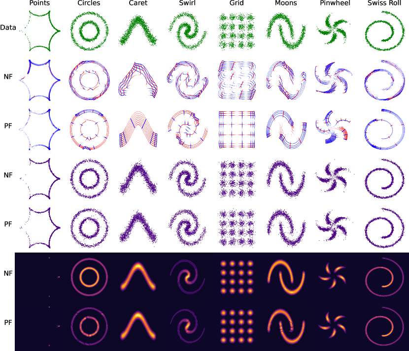
Refer to caption
Figure 7: Extended results for synthetic datasets. Top row has true samples, the next two rows are contours, the next two are samples and the last two are probability densities computed by the models.

See Fig.7 for extended results. Each dataset was generated with 1,000,000 data points and split into 700,000 for training and 300,000 for testing. As mentioned in the main text, the architecture used on all of the datasets consisted of 10 coupling layers with logistic mixture cdf layers that used 8 mixture components and an affine coupling layer that shared the same conditioner network. Each conditioner consisted of 5 residual layers with a hidden layer size of 64. The models were trained using the AdaBelief [Zhuang et al., 2020] optimization algorithm with a learning rate of 1×1031superscript1031\times 10^{-3} and a batch size of 256, and α=10.0𝛼10.0\alpha=10.0. Each model was trained for approximately 4 hours on either a NVIDIA 1080ti or 2080ti.

D.2 Variable dimension manifold

We used a flow with 20 coupling based neural spline [Durkan et al., 2019] layers, each with 8 knot points, followed directly by an affine coupling layer that is parametrized by the same conditioner network as done in [Ho et al., 2019]. The conditioner networks all consisted of a 5 layer residual network with a hidden dimension of 32. We used a unit Gaussian prior. The model was trained for around 4 hours on a NVIDIA 3090 gpu with a learning rate of 1×1041superscript1041\times 10^{-4} with the AdaBelief [Zhuang et al., 2020] optimization algorithm and a batch size of 2048 and α=5.0𝛼5.0\alpha=5.0. We trained on 2,100,000 data points and evaluated on 900,000. As stated in the main text, the data was augmented with Gaussian noise with a standard deviation of 0.01 to ensure that the model did not collapse during training. The true generative model for the data is:

z1subscript𝑧1\displaystyle z_{1} 13(N(2,0.3)+N(0,0.3)+N(2,0.3))similar-toabsent13𝑁20.3𝑁00.3𝑁20.3\displaystyle\sim\frac{1}{3}(N(-2,0.3)+N(0,0.3)+N(2,0.3)) (74)
z2subscript𝑧2\displaystyle z_{2} N(0,1)similar-toabsent𝑁01\displaystyle\sim N(0,1) (75)
x𝑥\displaystyle x =f(z1,z2)=[z1z2max(0,1|1z1|)sin(z1)]absent𝑓subscript𝑧1subscript𝑧2matrixsubscript𝑧1subscript𝑧2max011subscript𝑧1subscript𝑧1\displaystyle=f(z_{1},z_{2})=\begin{bmatrix}z_{1}\\ z_{2}\text{max}(0,1-|\frac{1}{z_{1}}|)\\ \sin(z_{1})\end{bmatrix} (76)

The true density was computed in a piecewise manner. If x1=0subscript𝑥10x_{1}=0, then

p(x)=p(z1)|df(z)dz1Tdf(z)dz1|12𝑝𝑥𝑝subscript𝑧1superscriptsuperscript𝑑𝑓𝑧𝑑subscript𝑧1𝑇𝑑𝑓𝑧𝑑subscript𝑧112\displaystyle p(x)=p(z_{1})|\frac{df(z)}{dz_{1}}^{T}\frac{df(z)}{dz_{1}}|^{\frac{-1}{2}} (77)

Otherwise,

p(x)=p(z1)p(z2)|df(z)dzTdf(z)dz|12𝑝𝑥𝑝subscript𝑧1𝑝subscript𝑧2superscriptsuperscript𝑑𝑓𝑧𝑑𝑧𝑇𝑑𝑓𝑧𝑑𝑧12\displaystyle p(x)=p(z_{1})p(z_{2})|\frac{df(z)}{dz}^{T}\frac{df(z)}{dz}|^{\frac{-1}{2}} (78)

The Jacobian determinants were computed with automatic differentiation.

In Fig. 8 we show a larger version of Fig. 5, in Fig. 9 we showcase samples pulled from the PF and the contours learned by the model. In Fig. 10 we see that the PF does extremely well in predicting the log likelihood of the test set. The final KL divergence between the true data distribution and learned was 0.0146. To choose the rank at test time, we compared the three contour likelihoods provided by the model and filtered out the likelihoods that were negligible compared to the others.
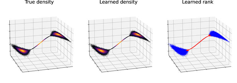
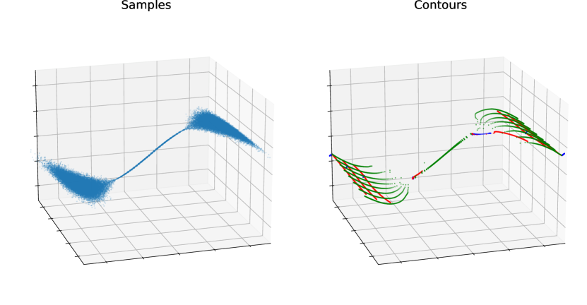
Refer to caption
Figure 8: A larger version of Fig. 5
Refer to caption
Figure 9: Samples and contours from the model trained for Section 5.2
Refer to caption
Figure 10: Histogram of the difference between the true log likelihood and the predicted for the experiment in Section 5.2

D.3 iPF

Preprocessing

For training, we preprocessed incoming batches of data using uniform dequantization and a scaling layer + logit transformation as described in [Dinh et al., 2017]. Then each (28×28×1)28281(28\times 28\times 1) image was flattened into a 784 dimensional vector.

Model architectures

The iPF and iNF architectures were composed of two parts. The first is a flow in the full 784 dimensional ambient space that consisted of 20 layers of GLOW [Kingma and Dhariwal, 2018] with each conditioner network consisting of 3 residual networks with a hidden dimension of 32 and dropout rate of 0.2. After the GLOW layers, the output was sliced so that the resulting dimensionality was 10 and this low dimensional vector was passed to a unit Gaussian prior.

The second part of the architecture, used during fine-tuning, consisted of 10 coupling based neural spline layers with 8 knots and affine coupling layers. Each conditioner contained 4 residual network layers with a hidden dimension of 4. The input to this flow is the 10 dimensional output of the first component and the output is fed into a unit Gaussian prior.

Training

The overall model was trained in two stages. The first stage optimized the objective in section 4 of [Caterini et al., 2021] using only the GLOW layers. The objectives we optimized were:

Objective1iPFsubscriptObjective1iPF\displaystyle\text{Objective1}_{\text{iPF}} =𝐱𝒟logp𝐳(g(𝐱))+dim(𝐳)2log(iJki(g(𝐱))2)+γf(g(𝐱))x2,kUniform(1,,10)formulae-sequenceabsentsubscript𝐱𝒟subscript𝑝𝐳𝑔𝐱dimension𝐳2subscript𝑖subscript𝐽𝑘𝑖superscript𝑔𝐱2𝛾superscriptnorm𝑓𝑔𝐱𝑥2similar-to𝑘Uniform110\displaystyle=\sum_{\mathbf{x}\in\mathcal{D}}-\log p_{\mathbf{z}}(g(\mathbf{x}))+\frac{\dim(\mathbf{z})}{2}\log(\sum_{i}J_{ki}(g(\mathbf{x}))^{2})+\gamma||f(g(\mathbf{x}))-x||^{2},\quad k\sim\text{Uniform}(1,\dots,10) (79)
Objective1iNFsubscriptObjective1iNF\displaystyle\text{Objective1}_{\text{iNF}} =𝐱𝒟logp𝐳(g(𝐱))+12log|J(g(𝐱))TJ(g(𝐱))|+γf(g(𝐱))x2absentsubscript𝐱𝒟subscript𝑝𝐳𝑔𝐱12𝐽superscript𝑔𝐱𝑇𝐽𝑔𝐱𝛾superscriptnorm𝑓𝑔𝐱𝑥2\displaystyle=\sum_{\mathbf{x}\in\mathcal{D}}-\log p_{\mathbf{z}}(g(\mathbf{x}))+\frac{1}{2}\log|J(g(\mathbf{x}))^{T}J(g(\mathbf{x}))|+\gamma||f(g(\mathbf{x}))-x||^{2} (80)

For both models we set γ=10𝛾10\gamma=10, used a batch size of 64, learning rate of 1×1041superscript1041\times 10^{-4} and the AdaBelief [Zhuang et al., 2020] optimization algorithm. We found that it was crucial to use a small learning rate, otherwise training would fail. These models were trained for approximately 36 hours on either a NVIDIA 3090ti or RTX8000 gpu.

After this stage of training, we combined the GLOW layers with the neural spline layers into one normalizing flow. We then froze the parameters for the GLOW layers and trained the parameters of the spline layers using a learning rate of 1×1031superscript1031\times 10^{-3} for another 24 hours on the same objective as before, but without the reconstruction error term:

Objective2iPFsubscriptObjective2iPF\displaystyle\text{Objective2}_{\text{iPF}} =𝐱𝒟logp𝐳(g(𝐱))+dim(𝐳)2log(iJki(g(𝐱))2),kUniform(1,,10)formulae-sequenceabsentsubscript𝐱𝒟subscript𝑝𝐳𝑔𝐱dimension𝐳2subscript𝑖subscript𝐽𝑘𝑖superscript𝑔𝐱2similar-to𝑘Uniform110\displaystyle=\sum_{\mathbf{x}\in\mathcal{D}}-\log p_{\mathbf{z}}(g(\mathbf{x}))+\frac{\dim(\mathbf{z})}{2}\log(\sum_{i}J_{ki}(g(\mathbf{x}))^{2}),\quad k\sim\text{Uniform}(1,\dots,10) (81)
Objective2iNFsubscriptObjective2iNF\displaystyle\text{Objective2}_{\text{iNF}} =𝐱𝒟logp𝐳(g(𝐱))+12log|J(g(𝐱))TJ(g(𝐱))|absentsubscript𝐱𝒟subscript𝑝𝐳𝑔𝐱12𝐽superscript𝑔𝐱𝑇𝐽𝑔𝐱\displaystyle=\sum_{\mathbf{x}\in\mathcal{D}}-\log p_{\mathbf{z}}(g(\mathbf{x}))+\frac{1}{2}\log|J(g(\mathbf{x}))^{T}J(g(\mathbf{x}))| (82)
Refer to caption
Figure 11: Random samples from the iPF and injective normalizing flow trained in Section 5.3

Appendix E Practical considerations

PFs have many nice theoretical properties, but can be difficult to train and interpret in practice. We find that the constraint 𝒫=0subscript𝒫0\mathcal{I}_{\mathcal{P}}=0 can only be satisfied with normalizing flows that are very expressive. We conjecture that the reason is because the constraint 𝒫=0subscript𝒫0\mathcal{I}_{\mathcal{P}}=0 requires that each O(2|𝒫|)𝑂superscript2𝒫O(2^{|\mathcal{P}|}) possible contour that can be constructed are orthogonal to the other contours. As a result, we find it necessary to keep |𝒫|𝒫|\mathcal{P}| small by using iPFs to model high dimensional data, increasing the size of each partition or using a feature extractor flow that can transform data into a simpler form for the PF. Furthermore, the latent space of PFs is not trivial to interpret. While it is true that the latent variables of PFs correspond to different principal manifolds, the index of the dimension corresponding to different principal manifolds can change (see Fig. 4 for clear examples of this). This means that a smooth path through over a principal manifold may require a discontinuous path through the latent space.