Statistical inference for intrinsic wavelet estimators of SPD matrices in a log-Euclidean manifold

Abstract

In this paper we treat statistical inference for an intrinsic wavelet estimator of curves of symmetric positive definite (SPD) matrices in a log-Euclidean manifold. This estimator preserves positive-definiteness and enjoys permutation-equivariance, which is particularly relevant for covariance matrices. Our second-generation wavelet estimator is based on average-interpolation and allows the same powerful properties, including fast algorithms, known from nonparametric curve estimation with wavelets in standard Euclidean set-ups.

The core of our work is the proposition of confidence sets for our high-level wavelet estimator in a non-Euclidean geometry. We derive asymptotic normality of this estimator, including explicit expressions of its asymptotic variance. This opens the door for constructing asymptotic confidence regions which we compare with our proposed bootstrap scheme for inference. Detailed numerical simulations confirm the appropriateness of our suggested inference schemes.

1 Introduction

In this paper we derive statistical inference for an intrinsic wavelet estimator of a curve of positive definite matrices in a log-Euclidean manifold. This estimator preserves, among other interesting properties, the essential property of remaining itself positive-definite (PD). The paradigm of our approach is that this preservation of PD is possible without any pre- or postprocessing step, e.g. finding the PD estimator coming closest to the proposed wavelet estimator. Such a device would be prohibitive for a feasible analysis of its statistical properties (in particular mean-square convergence and asymptotic normality of the final estimator).

Some recent work (e.g. Pennec [2006], Hinkle et al. [2014]) on using differential-geometric tools in nonparametric estimation of matrix-valued curves opened an elegant and mathematically sound way of how to transfer powerful modern non-parametric curve estimation schemes from the classical situation only involving Euclidean distances to the world of non-flat manifolds, i.e. curved spaces. A prominent example is the space of symmetric and positive-definite (SPD) matrices which we will focus upon here. Important applications for curves with such matrix-valued entries are covariance matrices (with arguments changing over time or space, e.g.), but also diffusion tensors (Zhu et al. [2009], Dryden et al. [2009]): Diffusion tensor imaging (DTI) can be used in clinical applications to obtain high-resolution information of internal structures of pathological versus healthy tissues of certain organs (e.g. hearts and brains). For each tissue voxel, there is a 3 x 3 SPD matrix to describe the shape of local diffusion. Other scientific applications of SPD matrices, finally, are numerous, such as in computer vision Caseiro et al. [2012], elasticity Moakher [2006], signal processing Arnaudson et al. [2013], medical imaging (Fillard et al. [2007]), Fletcher and Joshib [2007]) and neuroscience Friston [2011].

In Chau and von Sachs [2021a] the slightly larger class of Hermitian positive-definite (HPD) matrices has been studied, with as prominent examples, spectral density matrices of multivariate time series which are functions of frequency (or even of time and frequency for locally stationary time series with a time-varying correlation structure as in Chau and von Sachs [2021b]). It is merely for reasons of keeping the presentation sufficiently light that we restrict ourselves, in this paper, to the class of SPD matrices.

The essential key to success for the aforementioned transfer to curved spaces hinges on the following idea. Evaluating the performance of usual nonparametric curve estimation builds on measuring the distance, and hence the speed of convergence, of an estimator to the target curve by the standard Euclidean metric. Hence it is important to replace the latter by a suitable metric that takes into account the structure of the underlying manifold.

While the work by Chau and von Sachs [2021a] concentrated on the use of the affine-invariant Riemannian metric, in this paper we consider the log-Euclidean metric to be at the base of our derivations. It provides a different natural distance between two SPD matrices, while still allowing to preserve some interesting invariance properties. In particular, the log-Euclidean metric transforms the space of SPD matrices in a complete metric space, and it is unitary congruence invariant (see also Lemma 11.9 in the Supplement 11). This implies equivariance of our constructed estimators with respect to, e.g., rotations, and has as the following important application in the use of the log-Euclidean metric for estimation of covariance matrices of a multivariate data vector (e.g. a time series): if the coordinates of the entries of the data vector are permuted, the estimator of its covariance matrix follows this permutation - a property lacking for other choices, such as, e.g., the Cholesky and the log-Cholesky metrics (Lin [2019]).

Using the log-Euclidean metric, most importantly, opens the way to derive properly centered asymptotic normality of the proposed curve estimators. We will subsequently use this in order to construct correctly centered confidence regions, due to the simplified geometric structure of the log-Euclidean compared to other Riemannian manifolds. Another advantage is that estimators based on this metric do not suffer from the swelling effect - which means that the determinant of an average of two (or more) SPD matrices in this metric is guaranteed to not exceed the determinant of any of the averaged matrices. This property will guarantee that our constructed confidence regions which are based on estimators that are constructed as intrinsic averages in our space of SPD matrices, will not swell either towards or beyond the borders of our manifold. This is obviously an important advantage for constructing confidence volumes not simply based on the Euclidean metric in order to have them respect the nominal level in practice without becoming incorrectly too large.

The relevant literature from the field of differential geometry on the theory of SPD matrices is vast (e.g. Arsigny et al. [2007], Pennec [2006]), and in this paper we restrict ourselves to review the aspect that are necessary for our approach. Essentially the idea is to relate a non-flat or curved space - which is supposed to contain both the matrix-valued curved to be denoised and the estimator that provides this denoising - with a classical Euclidean geometry that allows the control of distances. Mathematically speaking this is achieved by studying, locally for each element of the curved space, its tangent space. There are many possibilities to do this, most of them are based on differential-geometric tools such as the Exponential mapping - and its inverse - between the manifold and its tangent space. Among these, we decided to choose the log-Euclidean approach, in which the considered distances only depend on the matrix-logarithm of our objects.

As another paradigm of our work we want to benefit from the powerful properties of denoising observed curves by wavelet estimators (see, e.g., Antoniadis et al. [1994]). However, as our observed curves are matrix-valued, classical wavelet algorithms cannot be directly applied. Using the log-Euclidean metric allows us to build our work on a particular second-generation wavelet scheme (for general such schemes we refer, e.g. to Jansen and Oonincx [2005]), similarly to the one developed in Chau and von Sachs [2021a], as an important modification of the approach of Rahman et al. [2005]. This scheme is based on Average-Interpolation (AI), which is known to have powerful properties as developed, e.g. in Daubechies and Lagarias [1991],Daubechies and Lagarias [1992b] and Daubechies and Lagarias [1992a]. Moreover Donoho [1993] showed that wavelet estimators based on AI carry the same desirable properties as first-generation wavelet schemes. Those allow us to control not only rates of convergence of our intrinsic wavelet estimator but go beyond this in the study of its (asymptotic) variance in our newly derived central limit theorem. By construction and, again, use of the log-Euclidean metric which avoids any swelling effects, this enables us to construct appropriate confidence regions for points on the curve with values in the space of SPD matrices.

With our contribution we complete an important gap on statistical inference for wavelet-based curve estimators on non-standard geometries. Related statistical work exists in the context of local polynomial estimation (Yuan et al. [2012], wavelet estimation (Rahman et al. [2005]), and more generally for regression on Riemannian manifolds (Boumal and Absil [2011], Hinkle et al. [2014]), the latter references not providing any convergence rates of a statistical error measure (such as the mean-squared error). However, in this work we focus on providing confidence regions, both based on asymptotic normality and, for comparison and in its own interest, based on a bootstrap scheme. Beyond our detailed theoretical investigations we convince ourselves by extended simulation studies about the appropriateness of our suggested inference methods.

The rest of the paper is organized as follows. The notation and abbreviations are given in Section 2. We lay out conceptual details of differential geometry and intrinsic average interpolation in Section 3. The results for wavelet estimation in our nonparametric regression setup of denoising SPD-matrix valued curves are given in Section 4, i.e. reviewing rates of mean-square convergence, and foremost, deriving asymptotic normality including an explicit calculation of the asymptotic variance of our estimators. Section 5 presents the two different constructions of our confidence sets which live in the considered non-flat space of SPD-matrix valued curves. Here we base ourselves, on the one hand, on the shown asymptotic normality, and on the other hand, on a newly proposed (wild) bootstrap scheme, for which we show its theoretical validity. Finally we provide numerical simulation studies in Section 6, which show the satisfactory empirical coverage and a comparison between bootstrap confidence regions and those based on asymptotic normality. A short conclusion Section 7 sketches some possible extensions for future work.

All technical details are given in a Supplement which is structured as follows: First, in Section 8 we give further insights on the construction of our AI-wavelet scheme of section 3, including some proofs. Then we proceed to proving our statistical results of sections  4 and  5 in Sections 9 and 10, respectively. The Section 11 contains further material regarding the log-Euclidean metric.

2 Preliminaries

As outlined in the introduction this work is concerned with intrinsic curve estimation within the manifold $Sym^{+}(d)$ of $d\times d$ symmetric positive-definite (SPD) matrices. Now there are several ways to equip this differentiable manifold with a Riemannian metric, that is a positive definite inner product $g_{S}$ on the tangent space $T_{S}Sym^{+}(d)$ defined at each point $S\in Sym^{+}(d)$ and depending smoothly on $S$. We remark that $T_{S}Sym^{+}(d)$ can be identified with the ambient vector space $Sym(d)$ of symmetric matrices in the sense that both spaces are isomorphic. The most natural approach to obtain a Riemannian metric on $Sym^{+}(d)$ is then to simply restrict the Frobenius inner product on $Sym(d)$, which leads to the so called affine invariant metric, see Bhatia [2009] for a comprehensive treatment. Although geometrically very convenient, this metric imposes some computational difficulties when it comes to compute quantities such as Fréchet means. This is inherently due to the non-flatness of the resulting Riemannian manifold.
To circumvent some delicate issues that arise in inferential investigations on curved spaces, we instead consider the log-Euclidean metric, which was introduced in Arsigny et al. [2007] and provides a flat geometry on $Sym^{+}(d)$. A detailed exposition of the Riemannian structure induced by the log-Euclidean metric is provided in the Supplement, Section 11, of which we give a short summary in the following.

We start by collecting some notation: Let $M(d)$ denote the space of real $d\times d$ matrices and $GL(d)$ the subspace of invertible matrices. Then for any $A\in M(d)$, its matrix exponential is given by $\exp(A)=\sum_{k=0}^{\infty}A^{k}/k!\in GL(d)$. In particular the restriction $\exp\colon Sym(d)\to Sym^{+}(d)$ is one-to-one and for any $S\in Sym^{+}(d)$, there is a $\log(S)=A\in Sym(d)$ such that $\exp(A)=S$. The mapping $\log\colon Sym^{+}(d)\to Sym(d)$ is called (principal) matrix logarithm.
Then, choosing the Frobenius inner product $\langle A,B\rangle_{\mathrm{Id}}=\langle A,B\rangle_{F}=\mathrm{trace}(AB)$, $A,B\in Sym(d)$ in (11.1), the derivations in Section 11 lead to the following collection of geometric tools regarding the log-Euclidean metric:

$Sym^{+}(d)$	manifold
$T_{S}Sym^{+}(d)=S\times Sym(d)\cong Sym(d)$	tangent space
$g_{S}(U,V)=\mathrm{trace}(d_{S}\log(U)d_{S}\log(V)),\quad U,V\in T_{S}Sym^{+}(d)$	log-Eucl. metric
$d(S_{1},S_{2})=\|\log(S_{2})-\log(S_{1})\|_{F},\quad S_{1},S_{2}\in Sym^{+}(d)$	log-Eucl. distance
$\gamma(t;S_{1},S_{2})=\exp((1-t)\log(S_{1})+t\log(S_{2})),\quad S_{1},S_{2}\in Sym^{+}(d)$	geodesic
$\mathrm{Exp}_{S}(U)=\exp\big{(}\log(S)+d_{S}\log(U)\big{)},\quad S\in Sym^{+}(d),~{}U\in T_{S}Sym^{+}(d)$	exponential map
$\mathrm{Log}_{S_{1}}(S_{2})=d_{\log(S_{1})}\exp\big{(}\log(S_{2})-\log(S_{1})\big{)},\quad S_{1},S_{2}\in Sym^{+}(d)$	logarithmic map
$\Gamma_{S_{1}}^{S_{2}}(U)=d_{\log(S_{2})}\exp\big{(}d_{S_{1}}\log(U)\big{)},\quad S_{1},S_{2}\in Sym^{+}(d),~{}U\in T_{S_{1}}Sym^{+}(d)$	parallel transport
$\Gamma_{S}^{\mathrm{Id}}(U)=d_{S}\log(U),\quad S\in Sym^{+}(d),~{}U\in T_{S}Sym^{+}(d)$

Table 1: Abbreviations for the relevant differential geometric tools

Turning to the probabilistic aspects of our work, we recall, from the Hopf-Rinow theorem (i.e. Pennec [2006]), that $(Sym^{+}(d),\mathrm{d})$ is a complete separable metric space. Denote by $\mathcal{B}(Sym^{+}(d))$ the corresponding Borel $\sigma$-algebra, then we call a measurable function $X\colon(\Omega,\mathcal{A},\mathbb{P})\to(Sym^{+}(d),\mathcal{B}(Sym^{+}(d)))$ a random element on $Sym^{+}(d)$ and the induced probability measure $\mathbb{P}^{X}:=\mathbb{P}\circ X^{-1}$ on $Sym^{+}(d)$ is as usual referred to as the law or distribution of $X$.
Further, let $P(Sym^{+}(d))$ denote the set of all probability measures on $(Sym^{+}(d),$ $\mathcal{B}(Sym^{+}(d)))$ and $P_{m}(Sym^{+}(d))$ the subset of probability measures which have a finite moment of order $m$ with respect to the log-Euclidean distance $d$, i.e.

$$P_{m}(Sym^{+}(d)):=\left\{\nu\in P(Sym^{+}(d))\colon\int_{Sym^{+}(d)}d(S_{0},S)^{m}\,\mathrm{d}\nu(S)<\infty\right\},$$

where $S_{0}\in Sym^{+}(d)$ is arbitrary. We note in passing that we will use $\lambda$ to denote the Lebesgue measure on $\mathbb{R}$.

3 The intrinsic AI wavelet transform

This section is largely inspired by the developments in Chau and von Sachs [2021a], adapted to the particular situation of a log-Euclidean manifold. It addresses the three fundamental aspects of the present curve estimation problem. Due to the non-Euclidean set-up of SPD-matrix valued curves, we need to both develop how average-interpolation (AI) as a particular second generation schemes for wavelet estimation works for non-scalar valued curves, but also how this construction can be adapted to the log-Euclidean manifold. In order to do so, we first outline the geometric aspects of the present setting and provide the reader with some background on the intrinsic, i.e. the Fréchet mean for the log-Euclidean metric and its connection to average interpolation (for classical wavelet AI we refer to Klees and Haagmans [2000] and to Donoho [1993]). AI for wavelets provide multiscale representations and can successfully be implemented via refinement schemes, the basics of which we explain in the second part of this section. Here, in order to implement the predicting step that is inherent to all second generation schemes based on lifting (Jansen and Oonincx [2005]), we rely on predicting the midpoints of the refinement scheme by intrinsic average interpolation. In the third part, we detail the concept of forward and backward average interpolation (which provide the fast wavelet transform), hence our multiscale algorithm for processing observed data and their estimated local averages across different scales. Finally, in the fourth part, we discuss convergence of AI refinement schemes.

3.1 Fréchet means

Let $\mathbb{E}[X]$ or $\mu$ denote the Fréchet (or Karcher) mean of a random element $X$ on $Sym^{+}(d)$, which provides a general notion of location in metric spaces and is in our case defined as the set

$$\mathbb{E}[X]:=\operatorname*{arg\,min}_{R\in Sym^{+}(d)}\mathbb{E}[d^{2}(R,X)]=\operatorname*{arg\,min}_{R\in Sym^{+}(d)}\int_{Sym^{+}(d)}d^{2}(R,S)\,\mathrm{d}\mathbb{P}^{X}(S).$$

If $\mathbb{P}^{X}\in P_{2}(Sym^{+}(d))$, then at least one such point exists. Moreover, the Fréchet mean $\mathbb{E}[X]$ is unique because $Sym^{+}(d)$ is a geodesically complete and flat manifold with respect to the log-Euclidean metric. Since at every point $S\in Sym^{+}(d)$ the exponential map (see table 1) is defined on the entire tangent space $T_{S}Sym^{+}(d)$ the Fréchet mean $\mathbb{E}[X]\in Sym^{+}(d)$ is also uniquely characterized by the condition $\mathbb{E}[\mathrm{Log}_{\mu}(X)]=0$. The simple geometry under the log-Euclidean metric then allows to conclude

$$\mathbb{E}[X]=\exp(\mathbb{E}[\log(X)])\ ,$$

where $\mathbb{E}[\log(X)]$ is just the usual Euclidean expectation of the random matrix $\log(X)$ in the vector space $Sym(d)$. That is, for $\mathbb{P}^{\log(X)}=\mathbb{P}^{X}\circ\exp$, we have

$$\mathbb{E}[\log(X)]=\int_{Sym(d)}A\,\mathrm{d}\mathbb{P}^{\log(X)}(A)=\int_{Sym^{+}(d)}\log(S)\,\mathrm{d}\mathbb{P}^{X}(S).$$

If $X$ has a discrete distribution $\mathbb{P}^{X}=\sum_{i=1}^{n}w_{i}\delta_{S_{i}}$, where $\sum_{i}w_{i}=1$, $w_{i}>0$ and $S_{i}\in Sym^{+}(d)$, then

$$E[X]=\exp\left(\sum_{i=1}^{n}w_{i}\log(S_{i})\right)=:\mathrm{Ave}(\{S_{i}\};\{w_{i}\}),$$

see also Arsigny et al. [2007], Theorem 3.13. In case $w_{i}=1/n$ we may simply write $\mathrm{Ave}(\{S_{i}\})$ (or $\overline{S}_{n}$ resp. $\overline{X}_{n}$) for the average $\mathrm{Ave}(\{S_{i}\};\{1/n\})$.

Furthermore, if we consider a smooth curve $c\colon\mathbb{R}\supset I\to Sym^{+}(d)$ as a mapping from the probability space $(I,\mathcal{B}(I),\lambda/\lambda(I))$ to the 1-dimensional submanifold $c(I)\subset Sym^{+}(d)$ we can also define the intrinsic mean $\mathrm{Ave}_{I}(c)$ of $c$ by

$$\mathrm{Ave}_{I}(c):=\operatorname*{arg\,min}_{R\in c(I)}\int_{c(I)}d^{2}(R,S)\,\mathrm{d}\nu^{c}(S)$$

with $\nu^{c}:=\lambda/\lambda(I)\circ c^{-1}$. Again in case $\nu^{c}\in P_{2}(c(I))$, $\mathrm{Ave}_{I}(c)$ exists and is unique. Restricting the above considerations on the submanifold $c(I)$ we then obtain

$$\mathrm{Ave}_{I}(c)=\exp\left\{\int_{c(I)}\log(S)\,\mathrm{d}\nu^{c}(S)\right\}=\exp\left\{\frac{1}{\lambda(I)}\int_{I}\log(c(t))\,\mathrm{d}t\right\}.$$ (3.1)

3.2 Intrinsic average-interpolation refinement scheme

The data are assumed to stem from a curve $c\colon[0,1]\to Sym^{+}(d)$, which is square integrable in that $\int_{0}^{1}\|c(t)\|_{F}^{2}\,\mathrm{d}t<\infty$. As usual for nonparametric regression, the $n=2^{J}$ data observations $(c(k/2^{J}))_{k=0,\ldots,2^{J}-1}$ result from (noisy versions of) equidistant sampling of the curve $c(t)$ on a (dyadic) resolution scale $J$, i.e. for grid points $t_{k}=k/2^{J},k=0,\ldots,2^{J}-1$. As a common possibility for refinement schemes based on wavelets, those sampled data points are identified with the scaling coefficients $(M_{J,k})_{k}$ of the (wavelet) refinement scheme on the sampling (or finest) scale $J$. That is, the input data of the refinement scheme are the $(M_{J,k})_{k}$, observed on scale $J$, and satisfy the following deterministic relation

$$M_{J,k}=\mathrm{Ave}_{I_{J,k}}(c)=\exp\left\{2^{J}\int_{I_{J,k}}\log(c(t))\,\mathrm{d}t\right\},\quad k=0,\ldots,2^{J}-1,$$

where $I_{J,k}=2^{-J}[k,k+1)$ is a uniform partition of $[0,1)$.
We note that the intrinsic refinement scheme described in the following can also be adapted to a non-dyadic observation grid, see for instance Chau [2018].

In order to later utilize the refinement scheme for regression analysis the requirements for the scheme are two folded. On the one hand, refined or predicted midpoints have to form an average of coarser scale midpoints, so the transformation is suitable for noise-removal. On the other hand, the success of the refinement schemes hinges on the ability to reconstruct what is to be defined an intrinsic polynomial of a given degree without any error of approximation, akin the essential property that is enjoyed by wavelet schemes (of adapted order) in the classical setting. Similarly to the usual definition of a polynomial of degree $k$ to have vanishing derivatives of all orders $\ell\geq k$, here now a smooth curve $c\colon\mathbb{R}\supset[a,b]\to M$ on a manifold $M$ with existing (covariant) derivatives of all orders is said to be a polynomial curve or intrinsic polynomial of degree $k$, if all its derivatives of orders $\ell\geq k$ do vanish. For example a zero-degree polynomial is just a constant curve and a first-degree polynomial corresponds to a geodesic curve. For a more formal definition, we refer to Hinkle et al. [2014], see also Chau and von Sachs [2021a]. Unfortunately intrinsic $n$th-degree polynomials are in general difficult to express in closed form. However, and this will be important for our purposes, the unique interpolation polynomial passing through $S_{0},\ldots,S_{n}\in Sym^{+}(d)$ can be evaluated via an intrinsic version of Neville’s algorithm, see in the supplement, section 8 for details.

Now to derive a suitable refinement scheme that fits those requirements we adapt the average-interpolation (AI) refinement scheme as introduced in Donoho [1993] to the log-euclidean setup. That is, based on $j$-scale midpoints $(M_{j,k})_{k}$ the predicted or refined $(j+1)$-scale midpoints, denoted $(\widetilde{M}_{j+1,k})_{k}$, are computed as the $(j+1)$-scale midpoints of unique intrinsic polynomials with $j$-scale midpoints $(M_{j,k})_{k}$. To elaborate, let $N=2L+1$ for some $L\geq 0$ and fix a location $k\in\{L,\ldots,2^{j}-L\}$. The intrinsic AI-refinement scheme of order or degree $N$ is then formally defined as follows:
Let $\rho=\rho_{j,k}\colon[0,1]\to Sym^{+}(d)$ be the unique intrinsic polynomial (of degree $N-1$) with $j$-scale midpoints $M_{j,k-L},\ldots,M_{j,k+L}$, i.e.

$$\mathrm{Ave}_{I_{j,k^{\prime}}}(\rho)=\exp\left\{2^{j}\int_{k^{\prime}2^{-j}}^{(k^{\prime}+1)2^{-j}}\log(\rho(t))\,\mathrm{d}t\right\}=M_{j,k^{\prime}},\quad k^{\prime}=k-L,\ldots,k+L.$$

Then calculate the two predicted midpoints $\widetilde{M}_{j+1,2k}$ and$\widetilde{M}_{j+1,2k+1}$ on the next finer scale as

$$\widetilde{M}_{j+1,2k}=Ave_{I_{j+1,2k}}(\rho)=\exp\left\{2^{j+1}\int_{k2^{-j}}^{(2k+1)2^{-(j+1)}}\log(\rho(t))\,\mathrm{d}t\right\},$$

$$\widetilde{M}_{j+1,2k+1}=Ave_{I_{j+1,2k}}(\rho)=\exp\left\{2^{j+1}\int_{(2k+1)2^{-(j+1)}}^{(k+1)2^{-j}}\log(\rho(t))\,\mathrm{d}t\right\}.$$

Computing the integrals on the right hand side directly is of course infeasible, but similarly to AI-refinement on the real line, we can take advantage of the fact that the mean (in the sense of (3.1)) of an intrinsic polynomial is again an intrinsic polynomial to obtain tractable formulas for the predicted midpoints. To that end denote the cumulative intrinsic mean of $\rho$ by

$$\mathrm{Mean}(\rho;x):=\mathrm{Ave}_{[(k-L)2^{-j},x]}(\rho),\qquad x\in[(k-L)2^{-j},1].$$

Then, for $l=1,\ldots,2L+1=N$, a simple calculation shows that

$$\overline{M}_{j,l}:=\mathrm{Mean}(\rho;(k-L+l)2^{-j})=\mathrm{Ave}(M_{j,k-L},\ldots,M_{j,k-L+l}).$$

Furthermore we have

$$\mathrm{Mean}(\rho;(2k+1)2^{-(j+1)})= \exp\left\{\frac{2L}{2L+1}\log(\overline{M}_{j,L})+\frac{1}{2L+1}\log(\widetilde{M}_{j+1,2k})\right\}$$

$$= \gamma(\frac{1}{2L+1};\overline{M}_{j,L},\widetilde{M}_{j+1,2k}),$$ (3.2)

that is $\mathrm{Mean}(\rho;(2k+1)2^{-(j+1)})$ lies on the geodesic segment connecting $\overline{M}_{j,L}$ and $\widetilde{M}_{j+1,2k}$. Since $\mathrm{Mean}(\rho;\cdot)$ is by construction again an intrinsic polynomial of degree $N-1$ it can be reconstructed by a suitable polynomial interpolation. To that end let $\pi$ denote the intrinsic interpolation polynomial determined by the constrains

$$\pi((k-L+1)2^{-j})=\overline{M}_{j,l}=\mathrm{Ave}(M_{j,k-L},\ldots,M_{j,k-L+l}),$$

for $l=1,\ldots,N$. Then, due to the uniqueness of the interpolation polynomial, we have $\pi((2k+1)2^{-(j+1)})=\mathrm{Mean}(\rho;(2k+1)2^{-(j+1)})$ and (3.2) yields

$$\widetilde{M}_{j+1,2k}=\gamma(-2L;\pi((2k+1)2^{-(j+1)}),\overline{M}_{j,L}).$$ (3.3)

For the other predicted midpoint note that

$$\mathrm{Ave}(\widetilde{M}_{j+1,2k},\widetilde{M}_{j+1,2k+1})=M_{j,k}$$

and therefore solving for $\widetilde{M}_{j+1,2k+1}$ yields

$$\widetilde{M}_{j+1,2k+1}=\exp\left\{2\log(M_{j,k})-\log(\widetilde{M}_{j,2k})\right\}.$$ (3.4)

Derivations of (3.2) and (3.3) are provided in the supplement, section 8.

Faster midpoint prediction in practice. The AI refinement scheme (3.3) and (3.4) reduces in practice to elementary linear algebra, which is encoded in a vector of prediction coefficients. We show the derivation of these coefficients for $N=1$ and $N=3$. Let $(M_{j,k-L},\ldots,M_{j,k+L})$ be a given input on scale $j$.

(a) $N=1$ (i.e., $L=0$). The prediction scheme simply forwards the values from scale $j$ to scale $j+1$, viz.,

$$\widetilde{M}_{j+1,2k} =\exp\left\{\log(\pi((2k+1)2^{-(j+1)}))\right\}=\overline{M}_{j,k}=\mathrm{Ave}(M_{j,k})=M_{j,k},$$

$$\widetilde{M}_{j+1,2k+1} =\exp\left\{2\log(M_{j,k})-\log(\widetilde{M}_{j,2k})\right\}=M_{j,k}.$$

(b) $N=3$ (i.e, $L=1$) is the first non-trivial case. We show in Section 8.1

$$\widetilde{M}_{j+1,2k} =\exp\left\{\frac{1}{8}\log(M_{j,k-1})+\log(M_{j,k})-\frac{1}{8}\log(M_{j,k+1})\right\},$$ (3.5)

$$\widetilde{M}_{j+1,2k+1} =\exp\left\{-\frac{1}{8}\log(M_{j,k-1})+\log(M_{j,k})+\frac{1}{8}\log(M_{j,k+1})\right\}.$$ (3.6)

Carrying out these steps for general $L\geq 0$, i.e., $N=2L+1$, we obtain

$$\begin{split}\widetilde{M}_{j+1,2k}&=\mathrm{Ave}(\{M_{j,k-L},\ldots,M_{j,k+L}\},\\ &\qquad\qquad\{-c_{L},\ldots,-c_{1},1,c_{1},\ldots,c_{L}\})\\ \widetilde{M}_{j+1,2k+1}&=\mathrm{Ave}(\{M_{j,k-L},\ldots,M_{j,k+L}\},\\ &\qquad\qquad\{c_{L},\ldots,c_{1},1,-c_{1},\ldots,-c_{L}\})\end{split}$$ (3.7)

for suitable weights $(c_{1},\ldots,c_{L})$. In fact these weights are the same as in the average-interpolation transform in the Euclidean case (see Donoho [1993]). If $L=1$, $c_{1}=-1/8$ by the above derivation. If $L=2$, $(c_{1},c_{2})=(22,-3)/128$. If $L=3$, $(c_{1},c_{2},c_{3})=(-201,44,-5)/1024$.

3.3 Intrinsic forward and backward average-interpolation wavelet transform

The intrinsic AI-refinement scheme developed in the previous section naturally leads to a corresponding intrinsic AI wavelet transform that can be used to synthesize a smooth curve in $Sym^{+}(d)$. The first step in constructing a wavelet transform is to build up a redundant midpoint (or scaling coefficient) pyramid. The midpoint pyramid algorithm aggregates information from a finest observation scale $J$ successively to coarser scales. It is at the heart of the wavelet transform.

$$\begin{array}[]{cccccccccc}M_{J,0}&&M_{J,1}&M_{J,2}&&M_{J,3}&\cdots&M_{J,2^{J}-2}&&M_{J,2^{J}-1}\\ \searrow&&\swarrow&\searrow&&\swarrow&&\searrow&&\swarrow\\ &M_{J-1,0}&&&M_{J-1,1}&&\cdots&&M_{J-1,2^{J-1}-1}&\\ &\searrow&&&\swarrow&&&&\swarrow&\\ &&&&&\vdots&&&&\\ &&&&&\vdots&&&&\\ &&M_{2,0}&&M_{2,1}&&M_{2,2}&&M_{2,3}&\\ &&\searrow&&\swarrow&&\searrow&&\swarrow&\\ &&&M_{1,0}&&&&M_{1,1}&&\\ &&&\searrow&&&&\swarrow&&\\ &&&&&&&&&\\ &&&&&M_{0,0}&&&&\end{array}$$

Figure 1: Scheme of the midpoint pyramid algorithm. Each $M_{j,k}$ is obtained from $M_{j+1,2k}$ and $M_{j+1,2k+1}$ by the averaging procedure in (3.8), resulting in a consecutive finer average for a fixed $M_{j,k}$ in the case that the finest scale $J$ increases to $\infty$.

Midpoint pyramid. Consider midpoints $(M_{J,k})_{k=0}^{2^{J}-1}$ at the finest scale $J$ to be given by the sampled data. At the next coarser scale $j=J-1$ set $M_{j,k}$ to be the halfway point or midpoint on the geodesic $\gamma$ passing through $M_{j+1,2k}$ and $M_{j+1,2k+1}$, i.e.

$$\begin{split}M_{j,k}&:=\gamma(1/2;M_{j+1,2k},M_{j+1,2k+1})=\mathrm{Ave}(M_{j+1,2k},M_{j+1,2k+1})\end{split}$$ (3.8)

for $k=0,\ldots,2^{j}-1$. Continue this coarsening operation up to scale $j=0$ to obtain the midpoint pyramid $((M_{j,k})_{j,k}:0\leq j\leq J,0\leq k\leq 2^{j}-1)$, see also the scheme in Figure 1.

Now the above considerations lead to the following forward ($j\leadsto j-1$) and backward ($j-1\leadsto j$) AI-wavelet transform.

Forward wavelet transform. As input take the $j$-scale midpoints $(M_{j,k})_{k}$. The output is the sequence of $(j-1)$-scale midpoints $(M_{j-1,k})_{k}$ and $j$-scale wavelet coefficients $(D_{j,k})_{k}$. In detail, the forward transform works as follows.

1. Coarsen/predict.
   (i) Compute the $(j-1)$-scale midpoints $(M_{j-1,k})_{k}$ according to the midpoint relation (3.8).
   (ii) Select a refinement order $N=2L+1$, $L\geq 0$ and generate the predicted midpoints $(\widetilde{M}_{j,k})_{k}$ based on $(M_{j-1,k})_{k}$ via (3.3) and (3.4) respectively (3.7).

2. Difference. Define the wavelet coefficients $(D_{j,k})_{k}$ as an intrinsic difference according to

   $$D_{j,k}:=2^{-j/2}\mathrm{Log}_{\widetilde{M}_{j,2k+1}}(M_{j,2k+1})\in T_{\widetilde{M}_{j,2k+1}}Sym^{+}(d).$$ (3.9)

Remark 3.1.

By construction the wavelet coefficients live in different tangent spaces. However, in order to be able to compare the wavelet coefficients (e.g., with a given uniform threshold), parallel transporting them to the same tangent space at the identity results in so called whitened wavelet coefficients given by

$$\begin{split}\mathfrak{D}_{j,k}&:=\Gamma_{\widetilde{M}_{j,2k+1}}^{\mathrm{Id}}(D_{j,k})\\ &=2^{-j/2}\big{(}\log(M_{j,2k+1})-\log(\widetilde{M}_{j,2k+1})\big{)}\in T_{\mathrm{Id}}Sym^{+}(d)=Sym(d).\end{split}$$ (3.10)

Of course the ”length” of the vectors does not change, that is

$$g_{\widetilde{M}_{j,2k+1}}(D_{j,k},D_{j,k})=2^{-j}\|\log(M_{j,2k+1})-\log(\widetilde{M}_{j,2k+1})\|_{F}^{2}=\|\mathfrak{D}_{j,k}\|_{F}^{2}.$$

Backward wavelet transform. As input take the $(j-1)$-scale midpoints $(M_{j-1,k})_{k}$ and $j$-scale wavelet coefficients $(D_{j,k})_{k}$. The output is the sequence of $j$-scale midpoints $(M_{j,k})_{k}$. In detail, the backward transform is performed as follows.

1. Refine/predict. (i) Given the refinement order $N=2L+1$, $L\geq 0$, generate the odd predicted midpoints $(\widetilde{M}_{j,2k+1})_{k}$ for $k\in\{0,\ldots,2^{j-1}-1\}$ based on $(M_{j-1,k})_{k}$ via (3.4).
   (ii) Compute the odd $j$-scale midpoints $(M_{j,2k+1})_{k}$ for $k\in\{0,\ldots,2^{j-1}-1\}$ by reversing (3.9), i.e.,

   $$M_{j,2k+1}=\mathrm{Exp}_{\widetilde{M}_{j,2k+1}}(2^{j/2}D_{j,k}).$$ (3.11)

2. Complete. Compute the even $j$-scale midpoints $(M_{j,2k})_{k}$ through the midpoint relation (3.8) for $k\in\{1,\ldots,2^{j-1}-1\}$, i.e.,

   $$M_{j,2k}=\exp\left(2\log(M_{j-1,k})-\log(M_{j,2k+1})\right)$$ (3.12)

Thus, given the coarsest midpoint $M_{0,0}$ and the wavelet coefficient pyramid $(D_{j,k})_{j,k}$ for $j=0,\ldots,J$ and $k=0,\ldots,2^{j-1}-1$, the original input sequence $(M_{J,k})_{k}$ can be retrieved by repeating the reconstruction procedure (3.11) and (3.12) up to scale $J$.

3.4 Convergence of AI refinement schemes

The estimation procedure which we introduce in the subsequent section 4 will require multiple consecutive applications of the AI refinement scheme when lifting the wavelet estimator from a coarse scale $J_{0}$ to a finer scale $J$. To consider such iterative applications it turns out to be convenient to express the transformations (3.7) via suitable transition matrices. In particular this allows us to study the asymptotic behaviour of our wavelet estimator.
To elaborate, let us define for a generic $m\times n$ matrix $A=(a_{i,j})_{i,j}$, the blocked $md\times nd$ matrix $A_{\diagdown d}$ by

$$A_{\diagdown d}=(a_{i,j}I_{d})_{i,j},$$

where $I_{d}\in\mathbb{R}^{d\times d}$ is the identity matrix. This means $A_{\diagdown d}$ consists of block matrices each of these matrices being the $a_{i,j}$ multiple of the identity $I_{d}$. Using the weights $c_{i}$, $i\in\{1,\ldots,L\}$, we define the square matrices $E_{N},O_{N}\in\mathbb{R}^{(2N-1)\times(2N-1)}$, see equations ($E_{N}$) and ($O_{N}$) at the end of this section. (Notice that $E_{N}$ and $O_{N}$ are similar as $O_{N}=ZE_{N}Z$, where $Z=Z^{-1}$ with $Z=[e_{2N-1},\ldots,e_{1}]$ and $e_{i}$ being the $i$th standard basis (column) vector in $\mathbb{R}^{(2N-1)}$.) Then a careful observation shows that the AI refinement (3.7) can be described with $(E_{N})_{\diagdown d}$ resp. $(O_{N})_{\diagdown d}$ by

$$\begin{bmatrix}\log\widetilde{M}_{j+1,2k-2L}\\ \vdots\\ \log\widetilde{M}_{j+1,2k+2L}\end{bmatrix}=(E_{N})_{\diagdown d}\begin{bmatrix}\log M_{j,k-2L}\\ \vdots\\ \log M_{j,k+2L}\end{bmatrix},$$ (3.13)

$$\begin{bmatrix}\log\widetilde{M}_{j+1,2k-2L+1}\\ \vdots\\ \log\widetilde{M}_{j+1,2k+2L+1}\end{bmatrix}=(O_{N})_{\diagdown d}\begin{bmatrix}\log M_{j,k-2L}\\ \vdots\\ \log M_{j,k+2L}\end{bmatrix}.$$ (3.14)

Consequently, we have

Lemma 3.2.

For $m\geq 1$ and $p=0,\ldots,2^{m}-1$ we have

$$\begin{bmatrix}\log\widetilde{M}_{j+m,2^{m}k-2L+p}\\ \vdots\\ \log\widetilde{M}_{j+m,2^{m}k+2L+p}\end{bmatrix}=X_{m}X_{m-1}\ldots X_{1}\begin{bmatrix}\log M_{j,k-2L}\\ \vdots\\ \log M_{j,k+2L}\end{bmatrix}$$

with $X_{i}\in\{(E_{N})_{\diagdown d},(O_{N})_{\diagdown d}\}$, $i=1,\ldots,m$.

So, it is of crucial interest whether the sequences $X_{m}\cdot X_{m-1}\cdot\ldots\cdot X_{1}$ converge as $m$ increases to infinity. The answer is affirmative and follows from results in Daubechies and Lagarias [1991, 1992b] as well as Donoho [1993].
To see this, we have to first define

$$(\widehat{c}_{-2L},\ldots,\widehat{c}_{2L+1}):=(c_{L},-c_{L},\ldots,c_{1},-c_{1},1,1,-c_{1},c_{1},\ldots,-c_{L},c_{L})$$

The unique non-trivial solution of the two-scale difference equation

$$f(x)=\sum_{k}\widehat{c}_{k}f(2x-k),\qquad f\in L^{1}$$ (3.15)

is then given by the limit (that is an application ad infinitum) of the classical AI refinement scheme on the real line to the Kronecker sequence $(\delta_{0,k})_{k}$, see Donoho [1993] Theorem 2.1 and Daubechies and Lagarias [1992b] Theorem 2.2 for a detailed explanation. Let $\varphi_{L}$ denote this fundamental solution of (3.15). For further properties of $\varphi_{L}$, in particular its regularity, we refer to the aforementioned papers. Now the connection between $\varphi_{L}$ and the limit of products of the form $X_{m}\cdot X_{m-1}\cdot\ldots\cdot X_{1}$, is as follows:

For any $x\in[0,1]$ we have the binary expansion

$$x=\sum_{j=1}^{\infty}d_{j}(x)2^{-j},\qquad d_{j}(x)\in\{0,1\}.$$

Adapting the notation in Daubechies and Lagarias [1992b] let us define

$$T_{0}=ZE_{N}^{T}Z,\qquad T_{1}=ZO_{N}^{T}Z.$$

Then as a consequence of Theorem 2.2 in Daubechies and Lagarias [1992b] we have that all infinite products of $T_{0}$ and $T_{1}$ converge to the limit

$$\lim_{m\to\infty}T_{d_{1}(x)}T_{d_{2}(x)}\ldots T_{d_{m}(x)}=\begin{bmatrix}\varphi_{L}(x-2L)&\cdots&\varphi_{L}(x-2L)\\ \vdots&&\vdots\\ \varphi_{L}(x+2L)&\cdots&\varphi_{L}(x+2L)\end{bmatrix},$$

where $(d_{j}(x))_{j}$ are the coefficients of the binary expansion of $x\in[0,1]$. Now let

$$X_{d_{j}(x)}=\mathds{1}\{d_{j}(x)=0\}(E_{N})_{\backslash d}+\mathds{1}\{d_{j}(x)=1\}(O_{N})_{\backslash d}$$

then

$$X_{d_{1}(x)}^{T}X_{d_{2}(x)}^{T}\ldots X_{d_{m}(x)}^{T}=Z_{\backslash d}T_{d_{1}(x)}T_{d_{2}(x)}\ldots T_{d_{m}(x)}Z_{\backslash d}$$

and therefore the above convergence implies for each $x\in[0,1]$

$$\lim_{m\to\infty}X_{d_{m}(x)}\ldots X_{d_{2}(x)}X_{d_{1}(x)}=\begin{bmatrix}\varphi_{L}(x-2L)&\cdots&\varphi_{L}(x+2L)\\ \vdots&&\vdots\\ \varphi_{L}(x-2L)&\cdots&\varphi_{L}(x+2L)\end{bmatrix}_{\backslash d}=:\Phi_{L}(x)_{\backslash d}.$$ (3.16)

$$E_{N} :=\left[\begin{array}[]{ccccccccccccccccc}-c_{L}&-c_{L-1}&\cdots&-c_{1}&1&c_{1}&\cdots&c_{L-1}&c_{L}&0&&&&&&\\ c_{L}&c_{L-1}&\cdots&c_{1}&1&-c_{1}&\cdots&-c_{L-1}&-c_{L}&0&&&&&&\\ 0&-c_{L}&\cdots&-c_{2}&-c_{1}&1&\cdots&c_{L-2}&c_{L-1}&c_{L}&&&&&&\\ 0&c_{L}&\cdots&c_{2}&c_{1}&1&\cdots&-c_{L-2}&-c_{L-1}&-c_{L}&&&&&&\\ &&&\vdots&\vdots&\vdots&&\vdots&\vdots&\vdots&&&&&&\\ &&&0&-c_{L}&-c_{L-1}&\cdots&-c_{1}&1&c_{1}&\cdots&c_{L-1}&c_{L}&0&&\\ &&&0&c_{L}&c_{L-1}&\cdots&c_{1}&1&-c_{1}&\cdots&-c_{L-1}&-c_{L}&0&&\\ &&&&&&&\vdots&\vdots&\vdots&&\vdots&\vdots&&&\\ &&&&&&0&-c_{L}&-c_{L-1}&-c_{L-2}&\cdots&1&c_{1}&\cdots&c_{L}&0\\ &&&&&&0&c_{L}&c_{L-1}&c_{L-2}&\cdots&1&-c_{1}&\cdots&-c_{L}&0\\ &&&&&&&0&-c_{L}&-c_{L-1}&\cdots&-c_{1}&1&\cdots&c_{L-1}&c_{L}\end{array}\right] E_{N}$$ ()

$$O_{N} :=\left[\begin{array}[]{ccccccccccccccccc}c_{L}&c_{L-1}&\cdots&c_{1}&1&-c_{1}&\cdots&-c_{L-1}&-c_{L}&0&&&&&&&\\ 0&-c_{L}&\cdots&-c_{2}&-c_{1}&1&\cdots&c_{L-2}&c_{L-1}&c_{L}&&&&&&&\\ 0&c_{L}&\cdots&c_{2}&c_{1}&1&\cdots&-c_{L-2}&-c_{L-1}&-c_{L}&&&&&&&\\ &&&&\vdots&\vdots&&\vdots&\vdots&\vdots&&&&&&&\\ &&&0&c_{L}&c_{L-1}&\cdots&c_{1}&1&-c_{1}&\cdots&-c_{L-1}&-c_{L}&0&&&\\ &&&0&0&-c_{L}&\cdots&-c_{2}&-c_{1}&1&\cdots&c_{L-2}&c_{L-1}&c_{L}&&&\\ &&&&&&&\vdots&\vdots&\vdots&&\vdots&\vdots&\vdots&&&\\ &&&&&&&-c_{L}&-c_{L-1}&-c_{L-2}&\cdots&c_{1}&c_{2}&c_{3}&\cdots&c_{L}&0\\ &&&&&&&c_{L}&c_{L-1}&c_{L-2}&\cdots&-c_{1}&-c_{2}&-c_{3}&\cdots&-c_{L}&0\\ &&&&&&&0&-c_{L}&-c_{L-1}&\cdots&1&c_{1}&c_{2}&\cdots&c_{L-1}&c_{L}\\ &&&&&&&0&c_{L}&c_{L-1}&\cdots&1&-c_{1}&-c_{2}&\cdots&-c_{L-1}&-c_{L}\end{array}\right] O_{N}$$ ()

4 Wavelet regression for smooth curves in $Sym^{+}(d)$

Having introduced in the previous section the AI-wavelet scheme for SPD-matrix valued data, we can now describe our procedure of how to estimate smooth curves of symmetric PD matrices, observed in the presence of noise. For this we begin by introducing the data generating process given a certain curve $c\colon[0,1]\to Sym^{+}(d)$. Following the usual paradigm of (scalar) wavelet estimation, we set

$$M_{J,k}=\mathrm{Ave}_{I_{J,k}}(c)\ ,\;\;k\in\{0,\ldots,n-1\},$$

for $n=2^{J}$. We study an independent sample $M_{J,0,n},\ldots,M_{J,n-1,n}$ such that $M_{J,k,n}\sim\nu_{J,k}$ with $\nu_{J,k}\in P_{p}(Sym^{+}(d))$ and $\mathbb{E}_{\nu_{J,k}}[M_{J,k,n}]=M_{J,k}$ for a certain $p\geq 2$ given in (4.1). Moreover, to be consistent, we assume that the distributions of $M_{J,k,n}$ and $M_{J^{\prime},k^{\prime},n^{\prime}}$ are equal whenever $k2^{-J}$ and $k^{\prime}2^{-J^{\prime}}$ represent the same dyadic number. As an example consider the Riemannian signal plus noise model.

Example 1 (Riemannian signal plus noise model).

Suppose $c\colon[0,1]\to Sym^{+}(d)$ is an unknown target signal, $c_{k}=c(k/n)$, $k=0,\ldots,n$ and $\xi_{k}\sim\tilde{\nu}$ are i.i.d. mean-zero noise random variables in $Sym(d)$, $\tilde{\nu}\in P^{2}(Sym(d))$. We will consider the intrinsic signal plus noise model as a running example (see also Equation 2.2.17 in Chau [2018]) in the following.

$$X_{k} =\mathrm{Exp}_{c_{k}}(\Gamma_{\mathrm{Id}}^{c_{k}}(\xi_{k}))=\exp(\log(c_{k})+\xi_{k}),\quad k=0,\ldots,n.$$

The estimation procedure. Given input data on a dyadic scale, we obtain a smoothed curve as follows.

• Let $X=(X_{k})_{k=0,\ldots,n-1}$ be a sequence on the dyadic scale $J$ such that $2^{J}=n$.

• Denote $(M_{j,k,n})_{j,k}$ the midpoint pyramid according to (3.8) based on $X$. The empirical wavelet coefficients are $\widehat{D}_{j,k,n}$ for $j\in\{0,\ldots,J\}$ and $k\in\{0,\ldots,2^{j}-1\}$. We obtain these from the (estimated) predicted midpoints via (3.3), (3.4) and (3.9) for some refinement order $N=2L+1,L\geq 0$.

  In particular, on scale $J$, $M_{J,k,n}=X_{k}$ for $k\in\{0,\ldots,n-1\}$.

• The smoothing occurs at scales $j\in\{J_{0},\ldots,J\}$, where $J_{0}\in\{1,\ldots,J\}$ defines the thresholding scale for the empirical wavelet coefficients. We have

  $$\widehat{D}_{j,k,n}^{(t)}=\begin{cases}\widehat{D}_{j,k,n}&,j=0,\ldots,J_{0}-1\\ 0&,j=J_{0},\ldots,J\end{cases}\quad\text{for}~{}k=0,\ldots,2^{j-1}-1.$$

• Starting with $M_{0,0,n}$ and $\widehat{D}_{1,0,n}^{(t)}$ recursively apply the backward wavelet transform to obtain linearly thresholded estimated midpoints $(\widehat{M}_{j,k,n})_{j,k}$. At scale $J$, we obtain from $(\widehat{M}_{J,k,n})_{k}$ the curve $\hat{c}_{n}(t)=\sum_{k}\widehat{M}_{J,k,n}\mathds{1}_{I_{J,k}}(t)$.
  

The covariance operator. In order to study asymptotic normality and confidence regions, we need to model the covariance structure of the sampling scheme. We abbreviate the covariance operator of $\log M_{J,k,n}$ by

$${\cal C}(k2^{-J})\colon Sym(d)\to Sym(d).$$

We assume that $({\cal C}(u):u\in[0,1]\text{ is dyadic})$ can be extended to a càdlàg process $({\cal C}(u):u\in[0,1])\subset{\cal L}$ whose projections are positive definite in that $\langle A,{\cal C}(u)A\rangle_{F}>0$ for all $u\in[0,1]$. Here ${\cal L}={\cal L}(Sym(d))$ denotes the (Banach-) space of bounded linear operators $T\colon Sym(d)\to Sym(d)$ equipped with the usual induced operator norm $\|T\|_{\cal L}=\sup\{\|TA\|_{F}\mid A\in Sym(d),~{}\|A\|_{F}\leq 1\}$.

Furthermore, we assume a uniform bounded moments condition

$$c_{p}=\sup\mathbb{E}[\|\log M_{j,k,n}\|_{F}^{p}]<\infty,$$ (4.1)

for a $p>2$ and where the supremum is taken over $k\in\{0,\ldots,2^{j}-1\}$, $j\in\mathbb{N}$. This makes the process $({\cal C}(u):u\in[0,1])$ Bochner integrable, viz.,

$$\int_{0}^{1}{\cal C}(u)\mathop{}\!\mathrm{d}u\in{\cal L}.$$ (4.2)

Indeed, the Bochner integral exists if and only if $\int_{0}^{1}\|{\cal C}(u)\|_{{\cal L}}\mathop{}\!\mathrm{d}u<\infty$ as Lebesgue integral, this is satisfied in our model by the uniform bounded moments condition from (4.1) (see also Lemma 9.1).

Using that the inner product is bilinear and continuous in each argument, we can exchange the Bochner integral with the Lebesgue integral on any interval $I\subseteq[0,1]$

$$\int_{I}\langle A,{\cal C}(u)B\rangle\mathop{}\!\mathrm{d}{u}=\left\langle A,\int_{I}{\cal C}(u)\mathop{}\!\mathrm{d}{u}\ B\right\rangle$$

for $A,B\in Sym(d)$. This implies for each $A,B\in Sym(d)$ and $j\leq J$

$$\begin{split}&2^{-(J-j)}\sum_{u=0}^{2^{(J-j)}-1}\langle A,{\cal C}(k2^{-j}+u2^{-J})B\rangle\\ &\to\ 2^{j}\int_{k2^{-j}}^{(k+1)2^{-j}}\langle A,{\cal C}(u)B\rangle\mathop{}\!\mathrm{d}u=\left\langle A,2^{j}\int_{k2^{-j}}^{(k+1)2^{-j}}{\cal C}(u)\mathop{}\!\mathrm{d}uB\right\rangle\end{split}$$ (4.3)

as $J\to\infty$ for $j$ constant. In particular, for a small interval size, we can approximate the integral in (LABEL:E:ConvergenceCovOp) by $\langle A,{\cal C}(k2^{-j})B\rangle$ by the càdlàg property.

Example 2 (Continuation of example 1).

Note that in the signal plus noise model we have $\log M_{J,k,n}=\log(c_{k})+\xi_{k}$ and therefore

$$\mathrm{Cov}(\log M_{J,k,n})=\mathrm{Cov}(\xi_{k})=\mathcal{C}(k2^{-J})\equiv\cal C$$

for some $\cal C\in{\cal L}$. Hence the extension of the covariance operators is trivially given by $\mathcal{C}(u):=\mathcal{C},~{}u\in[0,1]$. Suppose the noise matrices $\xi_{k}$ have independent entries, that is

$$\xi_{k}=\sum_{1\leq i\leq j\leq d}z_{ij}^{k}E_{ij},$$

where $(z_{ij}^{k})_{i,j,k}$ are independent with $\mathbb{E}z_{ij}^{k}=0$ and $\mathrm{Var}(z_{ij}^{k})=\sigma_{ij}^{2}$. The matrices $E_{ij}\in Sym(d)$ are defined by

$$(E_{ij})_{k,l}=\begin{cases}1&,\quad i=k,j=l\ ~{}\text{or}\ ~{}i=l,j=k\\ 0&,\quad\text{else}\end{cases}$$

and obviously form a basis for $Sym(d)$.

Now $\mathcal{C}=\mathrm{Cov}(\xi_{k})\colon Sym(d)\to Sym(d)$ is a $4$th order tensor which can be represented (with respect to the standard basis) by an array $(C_{ijnm})_{i,j,n,m}$, i.e. $(\mathcal{C}A)_{i,j}=\sum_{n,m}C_{ijnm}A_{nm}$ for $A\in Sym(d)$. Since the covariance operator is uniquely characterized by $\langle\mathcal{C}A,A\rangle_{F}=\mathrm{Var}\langle\xi_{k},A\rangle_{F}$ for all $A\in Sym(d)$, writing out this equation yields

$$\sum_{i,j}\sum_{n,m}C_{ijnm}A_{nm}A_{ij}=\mathrm{Var}\sum_{i,j}(\xi_{k})_{ij}A_{ij}=\sum_{i,j}\mathrm{Var}(z_{ij}^{k})A_{ij}^{2}=\sum_{i,j}\sigma_{ij}^{2}A_{ij}^{2},$$

which in turn implies for the coefficients

$$C_{ijnm}=\begin{cases}\sigma_{ij}^{2}&,\quad i=n,j=m\ ~{}\text{or}\ ~{}i=m,j=n\\ 0&,\quad\text{else}.\end{cases}$$

A similar consideration shows that in the general case of dependent entries the coefficients of $\cal C$ are given by

$$C_{ijnm}=\mathrm{Cov}((\xi_{k})_{ij},(\xi_{k})_{nm})=:\sigma_{ijnm}.$$

Moreover due to the symmetry constraint $\sigma_{ijnm}=\sigma_{nmij}=\sigma_{mnij}=\sigma_{ijmn}$.

4.1 Asymptotics of the AI wavelet estimator

In order to derive our main result on asymptotic normality for the estimator $\widehat{M}_{J,k,n}$, it might be useful to first recall existing results on mean-square consistency of this estimator which result from the findings in Chau [2018] and Chau and von Sachs [2021a] for a general class of Riemannian metrics, including our considered log-Euclidean metric. We state here the corresponding result without a proof.

Proposition 4.1 (Rate of convergence from Chau and von Sachs [2021a] and Chau [2018] Appendix A).

Consider the wavelet estimator $\widehat{M}_{J,k,n}$, based on a refinement scheme of order $N$ and on (linear) thresholding on scale $J_{0}$. Let further $c(t)$ be a smooth curve of SPD matrices, possessing at least $N$ continuous derivatives. Then there is a $C\in\mathbb{R}_{+}$, which does not depend on $n$ and $k$ such that

$$\mathbb{E}[\|\log\widehat{M}_{J,k,n}-\mathbb{E}[\log\widehat{M}_{J,k,n}]\|_{F}^{2}]\leq C2^{-(J-J_{0})}$$

and

$$\|\mathbb{E}[\log\widehat{M}_{J,k,n}]-\log M_{J,k}\|_{F}\leq C2^{-NJ_{0}}.$$

In particular, the choice $J_{0}=\lfloor J/(2N+1)\rfloor\$ matches the variance and the squared bias, so

$$\mathbb{E}[d(\widehat{M}_{J,k,n},M_{J,k})^{2}]=\mathbb{E}[\|\log\widehat{M}_{J,k,n}-\log M_{J,k}\|_{F}^{2}]\leq 2Cn^{-2N/(2N+1)}\ ,$$

which implies that $\ n^{-1}\sum_{k=0}^{n-1}\mathbb{E}[d(\widehat{M}_{J,k,n},M_{J,k})^{2}]=O(n^{-2N/(2N+1)})$.

Now we turn to deriving asymptotic normality of the wavelet estimator which follows from the above lifting scheme and the following proposition.

Proposition 4.2 (Asymptotic normality of $\log M_{j,k,n}$).

Assume that the uniform bounded moments condition (4.1) is satisfied for a $p>2$.

• Let $j>0$ and let $0\leq k\leq 2^{j}-1$ be arbitrary but fixed. Then

  $$2^{-j/2}n^{1/2}(\log M_{j,k,n}-\mathbb{E}[\log M_{j,k,n}])\Rightarrow{\cal N}(0,\Sigma_{j,k}),\quad n=2^{J}\to\infty,$$

  on the Hilbert space $Sym(d)$ and the covariance operator $\Sigma_{j,k}$ is characterized by the condition

  $$\Sigma_{j,k}=2^{j}\int_{k2^{-j}}^{(k+1)2^{-j}}{\cal C}(u)\mathop{}\!\mathrm{d}u.$$

• Let $(J_{0,n},k_{n})_{n}$ be a sequence such that $J_{0,n}\to\infty$ and $J-J_{0,n}\to\infty$ and $k_{n}2^{-J_{0,n}}\to x\in[0,1]$, which is a point of continuity of ${\cal C}$. Then

  $$2^{-J_{0,n}/2}n^{1/2}(\log M_{J_{0},k,n}-\mathbb{E}[\log M_{J_{0},k,n}])\Rightarrow{\cal N}(0,{\cal C}(x)).$$

In order to quantify the limiting distribution of the wavelet estimator, we need additionally the limit

$$E_{N,\infty}=\lim_{m\to\infty}E_{N}^{m}=\Phi_{L}(0)\in\mathbb{R}^{(2N-1)\times(2N-1)},$$

see (3.16), and the corresponding quantity

$$\kappa_{N}:=\sum_{i=-2L}^{2L}(E_{N,\infty})^{2}_{1,i}=\sum_{i=-2L}^{2L}\varphi^{2}_{L}(i),$$ (4.4)

which enters into the variance of the Gaussian approximation.

Remark 4.3.

A factor of the form $\kappa_{N}$ is quite common to appear in the limit of wavelet estimators. We point out that for example (4.4) coincides with the term $w_{0}^{2}$ which appears in Theorem 3.4 in Antoniadis et al. [1994].

Theorem 4.4 (Asymptotic normality of the wavelet estimator).

Consider the wavelet estimator $\widehat{M}_{J_{n},k_{n},n}$ at a dyadic position $x\in(0,1)$ of the finest (sample) scale $J_{n}$, and let $J_{0,n}\to\infty$, $J_{n}-J_{0,n}\to\infty$, and $k_{n}2^{-J_{0,n}}\to x\in[0,1]$. Assume that $\cal C$ is continuous in $x$. Then for $p>2$

$$2^{-J_{0,n}/2}n^{1/2}(\log\widehat{M}_{J_{n},k_{n},n}-\mathbb{E}[\log\widehat{M}_{J_{n},k_{n},n}])\Rightarrow{\cal N}\Big{(}0,\kappa_{N}\ {\cal C}(x)\Big{)},\quad n\to\infty.$$

As usual with asymptotics ($n\to\infty$) for estimating curves sampled on an asymptotically finer and finer grid, one has to understand the above given expression for the asymptotic variance $\kappa_{N}C(x)$ in the sense that the reference location $x$ has to remain the same fixed dyadic rational in $(0,1)$ for all $n$.
In general, i.e. for $x$ not remaining the same fixed dyadic number, we are still be able to formulate a Central Limit Theorem of the following form:

Proposition 4.5.

Let $x\in(0,1)$ be not necessarily a dyadic number and assume the same regularity conditions as in Theorem 4.4. Then

$$Var(\langle A,\log\widehat{M}_{J_{n},k_{n},n}-\mathbb{E}[\log\widehat{M}_{J_{n},k_{n},n}]\rangle)^{-1/2}$$

$$\qquad\cdot(\langle A,\log\widehat{M}_{J_{n},k_{n},n}-\mathbb{E}[\log\widehat{M}_{J_{n},k_{n},n}]\rangle)\Rightarrow{\cal N}(0,1),\quad n\to\infty,$$

for any $0\neq A\in Sym(d)$.

Remark 4.6.

We shed a bit more light onto the fact that for non-dyadic numbers no stable limiting variance of the wavelet estimator may exist, and that we can only give the limiting behavior of the wavelet estimator in the “standardized” version of Proposition 4.5. This phenomenon has already been observed by Antoniadis et al. [1994], Theorem 3.3 and its discussion, for ordinary scalar-valued wavelet estimators. Essentially it is induced by the fact that for non-dyadic numbers on scale $j$ of the form $t_{j}=2^{j}t-[2^{j}t]\neq 0$, this sequence $t_{j}$ - and hence the asymptotic variance expressed as a function of this $t_{j}$ - fail to converge. In our situation this can be translated to non-convergence of the matrix products of the type $X_{J}\cdot X_{J-1}\cdot\ldots\cdot X_{J_{0}+1}$ with $X_{i}\in\{(E_{N})_{\diagdown d},(O_{N})_{\diagdown d}\}$, a representation occurring in Lemma 3.2 (see also (LABEL:E:NormalityLinEst2) in the Supplement). Recall that these products describe what happens if one lifts the AI wavelet estimator smoothed on scale $J_{0}$ from $J_{0}$ back to the sampling scale $J$. As both scales $J_{0}$ and $J$ need to tend to infinity simultaneously (though on different rates with $n$), convergence to finite limit depends on the fact whether there exists a $n_{0}$ beyond which the sequence $t_{n,0}:=k_{n}2^{-J_{0,n}}=x\in(0,1)$ for all $n>n_{0}$ (case of a dyadic point) or not: The affirmative case amounts to considering $J_{0}=J_{0,n}$ (i.e. the element $X_{J_{0}+1}$ in the matrix product) akin to remain fixed for all $n>n_{0}$, and the considered infinite matrix product possesses a limit (which is given by (3.16)). In the opposite case $X_{J_{0}+1}$ continues to change with $n$, leading to no convergence of the matrix product. By the proof of Proposition 4.5 we can, however, show that the behaviour remains somewhat controlled in this latter case.

With our derived Central Limit Theorem 4.4 we observe strong parallels in the given rates with those from classical nonparametric curve estimation. Choosing a scale $J_{0}<J$ is needed in order to collect enough statistical information for the estimation procedure using the midpoint pyramid algorithm, as the variance of a potential estimator on the initial scale $J$ would not decay. In order to increase the precision of the estimator, we also need the usual nonparametric conditions that $J=J_{0,n}\to\infty$ and $J_{n}-J_{0,n}\to\infty$, for which the precise asymptotic rates can be obtained as usual by matching the (squared) asymptotic bias and variance as in Proposition 4.1. Note, however, that this optimal choice $J_{0}=\lfloor J/(2N+1)\rfloor$ is merely of asymptotic flavour, as in practice, for reasonably small sample sizes $n=2^{J}$, this would lead to far too small scales $J_{0}$.

Remark 4.7.

Clearly, Theorem 4.4 is closely linked to Proposition 4.2 because the convergence to a Gaussian distribution is induced by the midpoint pyramid algorithm, which is applied in both statements. The main difference between both results consists in the final lifting step from the coarse scale $J_{0}$ back to the initial (sampling) scale $J$. This step rescales the limiting covariance operator from ${\cal C}(x)$ to $\kappa_{N}{\cal C}(x)$. Although we have not been able to prove, we conjecture that $\kappa_{N}<1$ if $L=(N-1)/2>1$ which shows a decrease of the value of the asymptotic variance. In the following we give a small discussion of the values of $\kappa_{N}$ for the first $N=1,3,5,7$:

If $L=0$, then the wavelet estimator simply corresponds to the $\log M_{J_{0},k,n}$. If $L=1$, i.e. $N=3$, we obtain for the limit of $\lim_{m\to\infty}E_{3}^{m}=E_{3,\infty}$ the matrix

$$E_{3}^{m} =\begin{pmatrix}\frac{1}{8}&1&-\frac{1}{8}&0&0\\ -\frac{1}{8}&1&\frac{1}{8}&0&0\\ 0&\frac{1}{8}&1&-\frac{1}{8}&0\\ 0&-\frac{1}{8}&1&\frac{1}{8}&0\\ 0&0&\frac{1}{8}&1&-\frac{1}{8}\end{pmatrix}^{m}\rightarrow\frac{1}{12}\begin{pmatrix}-1&7&7&-1&0\\ -1&7&7&-1&0\\ -1&7&7&-1&0\\ -1&7&7&-1&0\\ -1&7&7&-1&0\end{pmatrix}=E_{3,\infty}.$$

With some effort we were able to analytically compute $\kappa_{N}$ for some typical choices of $N$. The results are summarized in Table 2.

	$N=1$	$N=3$	$N=5$	$N=7$
$\kappa_{N}$	$1$	$\frac{25}{36}\approx 0.69$	$\frac{168549}{213160}\approx 0.79$	$\frac{107721892723}{126282847320}\approx 0.85$

Table 2:

5 Confidence sets for the wavelet estimator

In this section we develop confidence sets for our AI-based wavelet estimators of SPD matrix-valued curves, both based on the asymptotics of the previous section as well as on an appropriate form of a wild bootstrap scheme. It is in particular with the latter one that we propose some interesting inference method for non-scalar valued non-parametric curve estimators.

5.1 Asymptotic confidence sets

Our derived asymptotic $(1-\alpha)$-confidence sets are based on Proposition 4.2 and Theorem 4.4. In view of these results we rely on the log-normal distribution which we briefly recall here in the specific context of random matrices in $Sym^{+}(d)$.

Definition 5.1 (Log-normal distribution).

A random matrix $X\in Sym^{+}(d)$ has a log-normal distribution (w.r.t. the log-Euclidean metric) with mean $S\in Sym^{+}(d)$ and covariance operator $\Sigma\in{\cal L}$ if and only if

$$\langle\log X,A\rangle_{F}\sim\mathcal{N}(\langle\log S,A\rangle_{F},\langle\Sigma A,A\rangle_{F})\quad\forall A\in Sym(d).$$

Now a straightforward way to obtain distributional properties for log-normal random matrices is to utilize that $Sym(d)$ and $\mathbb{R}^{q}$, $q=d(d+1)/2$, are isometrically isomorphic. Consider the mapping $\eta\colon Sym(d)\to\mathbb{R}^{q}$ defined by

$$\eta(A):=(A_{11},\ldots,A_{dd},\sqrt{2}A_{12},\ldots,\sqrt{2}A_{1d},\sqrt{2}A_{23},\ldots,\sqrt{2}A_{2d},\ldots,\sqrt{2}A_{d-1,d})^{T}$$

for $\quad A=(A_{ij})_{ij}$. In other words $\eta$ stacks first the diagonal elements and than (row-wise) the above diagonal elements (scaled by $\sqrt{2}$) into a vector. Its easy to see that $\eta$ is one-to-one and $\langle\eta A,\eta B\rangle=\langle A,B\rangle_{F}$, thus, $\eta$ is an isometry. Moreover, a random matrix $X\in Sym^{+}(d)$ has a log-normal distribution in the sense of the definition if and only if

$$\eta(\log X)\sim\mathcal{N}(\eta(\log S),\widetilde{\Sigma})\quad with~{}~{}\widetilde{\Sigma}=\mathrm{Cov}(\eta(\log X))=\eta\Sigma\eta^{-1}.$$

This follows immediately since we have for arbitrary $a\in\mathbb{R}^{q}$ and $A=\eta^{-1}a\in Sym(d)$

$$\langle\eta(\log X),a\rangle=\langle\log X,A\rangle_{F} \sim\mathcal{N}(\langle\log S,A\rangle_{F},\langle\Sigma A,A\rangle_{F})$$

$$\sim\mathcal{N}(\langle\eta(\log S),a\rangle,\langle\eta\Sigma\eta^{-1}a,a\rangle),$$

i.e., $\eta(\log X)\sim\mathcal{N}(\eta(\log S),\tilde{\Sigma})$. Applying this insight to Proposition 4.2 (a) yields

$$2^{-j/2}\sqrt{n}\ \eta(\log M_{j,k,n}-\log M_{j,k})\Rightarrow\mathcal{N}(0,\widetilde{\Sigma}_{j,k}),$$

provided $\mathbb{E}[\log M_{j,k,n}]=\log M_{j,k}$ (which is true under for the Riemannian signal plus noise model from Example 1 and where $\widetilde{\Sigma}_{j,k}=\eta\Sigma_{j,k}\eta^{-1}$).

Now suppose that $\widehat{\widetilde{\Sigma}}_{j,k,n}$ is a consistent estimator for the covariance operator $\widetilde{\Sigma}_{j,k}$. As $\widetilde{\Sigma}_{j,k}^{-1/2}\mathcal{N}(0,\widetilde{\Sigma}_{j,k})$ agrees with $\mathcal{N}(0,I_{q\times q})$, we conclude with Slutsky’s theorem and the continuous mapping theorem

$$2^{-j}n\ \|\widehat{\widetilde{\Sigma}}_{j,k,n}^{-1/2}\eta(\log M_{j,k,n}-\log M_{j,k})\|^{2}$$

$$= 2^{-j}n\ \eta(\log M_{j,k,n}-\log M_{j,k})^{T}\ \widehat{\widetilde{\Sigma}}_{j,k,n}^{-1}\ \eta(\log M_{j,k,n}-\log M_{j,k})\Rightarrow\chi_{q}^{2}.$$

Therefore, if we let $\chi_{q,1-\alpha}^{2}$ denote the $(1-\alpha)$-quantile of the $\chi_{q}^{2}$ distribution, it follows that

$$CS_{n,1-\alpha}(M_{j,k})$$

$$:=\left\{S\in Sym^{+}(d)\mid 2^{-j}n\ \|\widehat{\widetilde{\Sigma}}_{j,k,n}^{-1/2}\ \eta(\log M_{j,k,n}-\log S)\|^{2}\leq\chi_{q,1-\alpha}^{2}\right\}$$

is an asymptotic $(1-\alpha)$-confidence set for $M_{j,k}$.

It is evident that this approach carries over to the wavelet estimator and that an asymptotic confidence set for $M_{J,k}$ at a dyadic point $x=k2^{-J}=k_{n}2^{-J_{n}}$ is in this case given by

$$\begin{split}&CS_{n,1-\alpha}(M_{J,k})\\ &:=\left\{S\in Sym^{+}(d)~{}\Bigg{|}~{}2^{J_{n}-J_{0,n}}\kappa_{N}^{-1}\|\widehat{\widetilde{\mathcal{C}}}(x)^{-1/2}\ \eta(\log\widehat{M}_{J_{n},k_{n},n}-\log S)\|^{2}\leq\chi_{q,1-\alpha}^{2}\right\}\end{split}$$ (5.1)

provided $\widehat{\widetilde{\mathcal{C}}}(x)$ is a consistent estimator for the covariance operator $\widetilde{\mathcal{C}}(x)=\eta\mathcal{C}(x)\eta^{-1}$. However, such an estimator can converge slowly in practice. Moreover, if the difference $J-J_{0}$ is not substantial the asymptotic confidence sets are expected to be rather conservative, which is also confirmed by simulations, see Section 6. These reasons motivate to consider confidence sets based on bootstrapping the wavelet estimator as an alternative.

Example 3 (Continuation of example 2).

Recall that in the signal plus noise model $M_{J,k,n}=\exp\{\log(c_{k})+\xi_{k}\}$ we have $\mathcal{C}(u)=\mathcal{C}=\mathrm{Cov}(\xi_{0}),~{}u\in[0,1]$. Furthermore, in case $\xi_{k}=\sum_{1\leq i\leq j\leq d}z_{ij}^{k}E_{ij}$, where $(z_{ij}^{k})_{i,j,k}$ are independent with $\mathbb{E}[z_{ij}^{k}]=0$ and $\mathrm{Var}(z_{ij}^{k})=\sigma_{ij}^{2}$, the coefficients of $\cal C$ (with respect to the standard basis) are simply

$$C_{ijnm}=\begin{cases}\sigma_{ij}^{2},&i=n,j=m~{}\text{or}~{}i=m,j=n\\ 0,&\text{otherwise}.\end{cases}$$

Thus, a straightforward calculation reveals

$$\widetilde{\mathcal{C}} =\eta\mathcal{C}\eta^{-1}=\mathrm{diag}(\sigma_{11}^{2},\ldots,\sigma_{dd}^{2},2\sigma_{12}^{2},\ldots,2\sigma_{1d}^{2},2\sigma_{23}^{2},\ldots,2\sigma_{2d}^{2},\ldots,2\sigma_{d-1,d}^{2}).$$

Now, let $m_{ij}^{(n)}=(\log M_{J_{n},k_{n},n})_{ij}$ and $a_{ij}=(\log S)_{ij}$. Then writing out the inequality in (LABEL:E:ConfidenceSetLinearEstimator) yields

$$2^{J_{n}-J_{0,n}}\kappa_{N}^{-1}\sum_{1\leq i\leq j\leq d}\frac{(m_{ij}^{(n)}-a_{ij})^{2}}{\sigma_{ij}^{2}}\leq\chi_{q,1-\alpha}^{2}$$

Viewed as an inequality in $(a_{ij})_{i,j}$ this subset of $Sym(d)$ corresponds (via the isometry $\eta$) to an ellipsoid in $\mathbb{R}^{q}$ with center

$$(m_{11}^{(n)},\ldots,m_{dd}^{(n)},\sqrt{2}m_{12}^{(n)},\ldots,\sqrt{2}m_{d-1,d}^{(n)})$$

and half-axis

$$\tau_{ij} =2^{(J_{0,n}-J_{n})/2}\sqrt{\kappa_{N}\sigma_{ij}^{2}\chi_{q,1-\alpha}^{2}},\quad 1\leq i\leq j\leq d.$$

If we denote this ellipsoid by $E((m_{ij}^{(n)},\tau_{ij})_{i,j},N,q,\alpha)$, we arrive at the compact representation

$$CS_{n,1-\alpha}(M_{J,k,n})=\left\{\exp(A)\mid A=\eta^{-1}(x),x\in E((m_{ij}^{(n)},\tau_{ij})_{i,j},N,q,\alpha)\right\}.$$

To illustrate, consider the case $d=2$. Then

$$CS_{n,1-\alpha}(M_{J,k})= \left\{\exp\left\{\begin{bmatrix}a_{11}&a_{12}/\sqrt{2}\\ a_{12}/\sqrt{2}&a_{22}\end{bmatrix}\right\}\Bigg{|}\begin{pmatrix}a_{11}\\ a_{22}\\ a_{12}\end{pmatrix}\in E((m_{ij}^{(n)},\tau_{ij})_{i,j},N,3,\alpha),\right\},$$

where

$$E((m_{ij}^{(n)},\tau_{ij})_{i,j},N,3,\alpha)= \left\{\begin{pmatrix}m_{11}^{(n)}+r_{11}\sin\theta\cos\varphi\\ m_{22}^{(n)}+r_{22}\sin\theta\cos\varphi\\ m_{12}^{(n)}+r_{12}\cos\theta\end{pmatrix}\Bigg{|}r_{ij}\in[0,\tau_{ij}],\theta\in[0,\pi],\varphi\in(-\pi,\pi]\right\}.$$

5.2 Wild bootstrap confidence sets

The resampling procedure works as follows. Let $J_{0}^{*}$ be a base level which is asymptotically coarser than $J$ in the sense that $J-J^{*}_{0}\to\infty$ and $J^{*}_{0}\to\infty$ as $n\to\infty$. Then generate a bootstrap estimator as follows.

• Given the initial observations $M_{J,k,n}$ obtain the sequence of wavelet estimators $\widehat{M}_{J^{*}_{0},J,k,n}$ w.r.t. the base level $J^{*}_{0}$.

• Calculate residuals $\hat{\varepsilon}^{*}_{J,k,n}=\log\widehat{M}_{J^{*}_{0},J,k,n}-\log M_{J,k,n}$, $k\in\{0,\ldots,2^{J}-1\}$.

• Simulate bootstrap residuals $\varepsilon^{boot}_{J,k,n}=\hat{\varepsilon}^{*}_{J,k,n}V_{J,k,n}$, where the $V_{J,k,n}$ are iid, real-valued random variables with mean zero and unit variance for $k\in\{0,\ldots,2^{J}-1\}$ and finite $(2+\delta)$th moment for some $\delta>0$.

• Create bootstrap observations $M^{boot}_{J,k,n}=\exp\Big{(}\log\widehat{M}_{J^{*}_{0},J,k,n}+\varepsilon^{boot}_{J,k,n}\Big{)}$ for each $k\in\{0,\ldots,2^{J}-1\}$.

• Compute $M^{boot}_{J_{0},k,n}$ for $k\in\{0,\ldots,2^{J}-1\}$ with the midpoint pyramid algorithm.

• Compute the wavelet estimator $\widehat{M}^{boot}_{J_{0},J,k,n}$ w.r.t. $J_{0}$ for $k\in\{0,\ldots,2^{J}-1\}$.

When simulating the residuals in (3) apart from a standard normal distribution, one can choose the two point distribution

$$V=\delta_{-\frac{\sqrt{5}-1}{2}}\cdot p+\delta_{\frac{\sqrt{5}+1}{2}}\cdot(1-p),$$

with $p=\frac{\sqrt{5}+1}{2\sqrt{5}}$. Then $V$ is the unique centered two point distribution which does not change the second and third moment, viz., $\mathbb{E}[V]=0$ and $\mathbb{E}[V^{3}]=\mathbb{E}[V^{2}]=1$.

Now, we consider the two processes

$$\mathfrak{M}_{J,k,n} =2^{-J_{0}/2}n^{1/2}(\log\widehat{M}_{J_{0},J,k,n}-\mathbb{E}[\log\widehat{M}_{J_{0},J,k,n}]),\quad n\in\mathbb{N},$$

$$\mathfrak{M}_{J,k,n}^{boot} =2^{-J_{0}/2}n^{1/2}(\log\widehat{M}^{boot}_{J_{0},J,k,n}-\mathbb{E}[\log\widehat{M}^{boot}_{J_{0},J,k,n}]),\quad n\in\mathbb{N}.$$

We have the following fundamental result.

Theorem 5.2 (Validity of the bootstrap).

Let the moment condition from (4.1) be satisfied for a $p>4$ and let $n=2^{J}$ as well as $J_{0},J_{0}^{*}\to\infty$ such that for some $\delta>0$

$$\min\Big{\{}(1-J_{0}^{*}/J)\frac{p}{2}-(1-J_{0}/J),(1-J_{0}/J)\frac{p}{4}\Big{\}}\geq(1+\delta)\text{ for all }n.$$

Let $x\in(0,1)$ be a dyadic rational and let $k/2^{J}=x$ eventually. Then with probability 1

$${\cal L^{*}}(\mathfrak{M}_{J,k,n}^{boot}) \Rightarrow{\cal N}\Big{(}0,\kappa_{N}\ {\cal C}(x)\Big{)},\quad n\to\infty,$$

conditionally on the data $\{M_{J,0,n},\ldots,M_{J,2^{J}-1,n}\}_{n}$. In particular,

$$\sup_{x\in Sym(d)}|\mathbb{P}(\mathfrak{M}_{J,k,n}\leq x)-\mathbb{P}^{*}(\mathfrak{M}_{J,k,n}^{boot}\leq x)|\to 0\quad a.s.,\quad n\to\infty$$

conditionally on the data. Here, for a random matrix $X$ with values in $Sym(d)$, we define the distribution function by $\mathbb{P}(X\leq x)=\mathbb{P}(X_{i,j}\leq x_{i,j},~{}\forall~{}1\leq i,j\leq d)$ for $x\in Sym(d)$.

Note that we need the moment condition from (4.1) to be satisfied for $p$ greater than 4 because this time we need in each setting a law of large numbers to hold for the empirical variance estimate.

Regarding the base level $J_{0}$, we observe that given $p>4(2N+1)/(2N)$, we can choose the optimal $J_{0}=\lfloor J/(2N+1)\rfloor$ as well as $J_{0}^{*}=\lfloor\alpha J\rfloor$ for

$$\alpha\in\Big{(}0,1-\frac{2}{p}\big{(}1+\frac{2N}{2N+1}\big{)}\Big{)}.$$

Note that the choice $\alpha=1/(2N+1)$ is admissible in this case. However, given these choices, we have to correct for the asymptotic bias $2^{(J-J_{0})/2}(\mathbb{E}[\log\widehat{M}_{J_{0},J,k,n}]-\log M_{J,k})$, which does not vanish in the limit given these choices.

Remark 5.3.

Concerning the choice of the base level $J_{0}$ we remark the following. When compared to the optimal choice $\lfloor J/(2N+1)\rfloor$ we distinguish two scenarios which already arise in bootstrap for traditional kernel regression. If $J_{0}-\lfloor J/(2N+1)\rfloor\to-\infty$, we oversmooth the estimator; conversely, if $J_{0}-\lfloor J/(2N+1)\rfloor\to\infty$, we undersmooth. Oversmoothing usually requires implicit or explicit bias correction and has been suggested in many contributions, see for instance the classical papers Härdle and Bowman [1988], Härdle and Marron [1991]. In order to avoid this need for bias correction undersmoothing is recommended (as addressed already in Hall [1992], Neumann [1994], Härdle et al. [2004]). In our present setting, and in particular for the simulated data examples in Section 6, undersmoothing is also favorable as the optimal choice $J_{0}=\lfloor J/(2N+1)\rfloor$ would be far too small even for moderate scales $J$.

Based on the above considerations we propose as bootstrap confidence sets

$$\begin{split}CS_{n,1-\alpha}^{boot}(\widehat{M}_{J,k})&:=\{S\in Sym^{+}(2)\mid d(\widehat{M}_{J,k},S)<r_{k}\}\\ &=\exp\left(\{A\in Sym(2)\mid\|\eta(\log\widehat{M}_{J,k})-\eta(A)\|<r_{k}\}\right)\\ &=\exp\left(\eta^{-1}\left(\{x\in\mathbb{R}^{3}\mid\|\eta(\log\widehat{M}_{J,k})-x\|<r_{k}\}\right)\right),\end{split}$$ (5.2)

i.e. the metric ball with centre $\widehat{M}_{J,k}$ and radius $r_{k}$ with respect to the log-Euclidean metric. The radius $r_{k}$ is taken as the $(1-\alpha)$-quantile of the distances

$$d(\widehat{M}_{J,k},~{}\widehat{M}_{J,k,b}^{boot})=\|\log\widehat{M}_{J,k}-\log\widehat{M}_{J,k,b}^{boot}\|,\qquad b=1,\ldots,B.$$

6 Numerical simulation examples

In this simulation study we test our proposed estimation procedure for the signal plus noise model $M_{J,k,n}=\exp\{\log(c_{k})+\xi_{k}\}$, where the noise matrices $\xi_{k}$ have independent Gaussian entries $z_{ij}^{k}\sim\mathcal{N}(0,\sigma_{ij}^{2})$, cf. example 2 and 3. We consider the following smooth $Sym^{+}(2)$-valued curves

$$c_{1}(t)=\begin{pmatrix}50\sqrt{1-(2t)^{2}}+0.1&2\sin(17\pi t)\\ 2\sin(17\pi t)&50t+1\end{pmatrix},$$

$$c_{2}(t)=\begin{pmatrix}55\cos(5\pi(t+0.1)/11)&50\sqrt{\sin(10\pi(t+0.1)/11)/2}\\ 50\sqrt{\sin(10\pi(t+0.1)/11)/2}&55\sin(5\pi(t+0.1)/11)\end{pmatrix},$$

$$c_{3}(t)=\begin{pmatrix}2(5-10t)^{2}&5-10t\\ 5-10t&1\end{pmatrix}$$

for $t\in[0,1]$ (see Figure 2).

For the different curves we choose the following variance parameters

$c_{1}\colon$	$\sigma_{11}=0.05$,	$\sigma_{22}=0.1$,	$\sigma_{12}=0.01$
$c_{2}\colon$	$\sigma_{11}=0.1$,	$\sigma_{22}=0.05$,	$\sigma_{12}=0.1$
$c_{3}\colon$	$\sigma_{11}=0.1$,	$\sigma_{22}=0.1$,	$\sigma_{12}=0.1$

For the different parameters of our AI-wavelet estimators we choose the order of the scheme to be moderate by taking $N=5$, the sample scale $J=10$ (i.e. a sample size of $n=1024$), and the smoothing scale $J_{0}<J$ to be the only remaining free parameter to be chosen curve by curve. For all simulations being based on $B=100$ bootstrap repetitions (for which we choose $J^{*}_{0}=J_{0}$), we compute first the wavelet estimator $(\widehat{M}_{J,k})_{k}$ and then the corresponding asymptotic (see (LABEL:E:ConfidenceSetLinearEstimator)) and bootstrap (see (5.2)) confidence sets - as derived in the previous section. Note that in (LABEL:E:ConfidenceSetLinearEstimator) we replace the estimated $\widehat{\widetilde{\cal{C}}}$ by the true $\widetilde{\cal{C}}$ (which is known in our simulation set-up) in order to minimize additional variability due to estimation of this variance parameter.

In order to visualize the results we identify positive definite matrices

$$M=\begin{pmatrix}x&z\\ z&y\end{pmatrix}$$

with points $(x,y,z)$ in the cone $C=\{(x,y,z)\in\mathbb{R}^{3}\mid xy>z^{2}\}$. Note that this correspondence is one-to-one. Both confidence sets are compared with respect to their empirical coverage based on $K=100$ samples and, since the confidence sets can be considered as subsets in the cone $C$, we also approximate their respective (Lebesgue-) volumes. To compensate for the dependency of the volumes on the location within the cone $C$ - close to the boundary for example the confidence sets are flattened out, and they generally grow larger with increasing distance from the origin - we also scale them by the volume that corresponds to the matrix exponential of the unit ball at the respective points.
Our simulations show that the wavelet estimator suffers from the classical bias phenomenon of non-parametric curve estimators at the boundaries. We therefore omit the first and last $100$ values in our computations. Moreover, in case of curve $c_{1}$ and $c_{2}$ we observe that our choice of $J_{0}=7$ and $J_{0}=5$, respectively, leads to satisfactory empirical coverages but also to a slightly too variable estimator. For this we refer to the discussion on undersmoothing in Remark 5.3. Finally, for curve $c_{3}$ we also observe a bias to appear around $t=1/2$ (where the curve almost touches the origin) - to be observed in Table 5 and Figure 8. To demonstrate that resulting empirical coverages for this curve are slightly lower only due to this phenomen, we also show another simulation set-up in Table 6 and Figure 9: here we center our confidence sets around the expected value of the wavelet estimator (instead of the true curve), which is approximated - at each considered point in time - by the sample mean over $50$ repetitions.

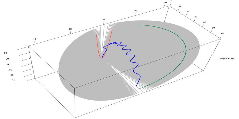
Figure 2: Cone $C$ and curves $c_{1}=$ blue, $c_{2}=$ green, $c_{3}=$ red.

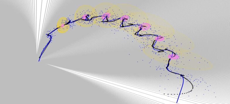
Figure 3: AI-wavelet estimator (black), asymptotic (gold) and bootstrap (pink) $0.9$-confidence sets for curve $c_{1}$ and $J=10$, $J_{0}=7$.

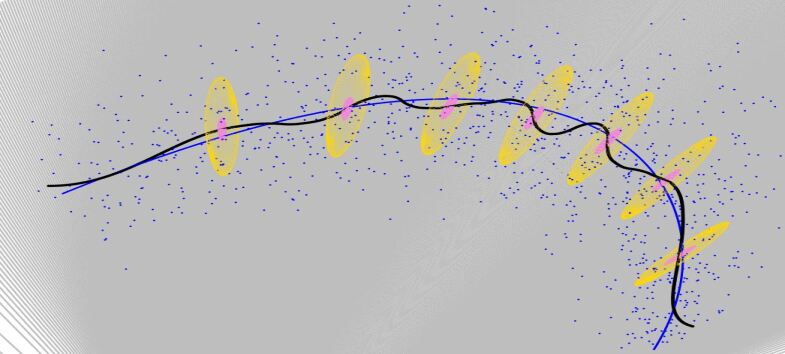
Figure 4: AI-wavelet estimator (black), asymptotic (gold) and bootstrap (pink) $0.9$-confidence sets for curve $c_{2}$ and $J=10$, $J_{0}=5$.

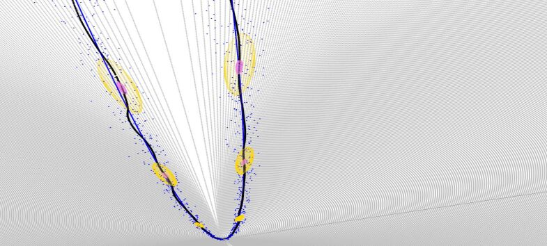
Figure 5: AI-wavelet estimator (black), asymptotic (gold) and bootstrap (pink) $0.9$-confidence sets for curve $c_{3}$ and $J=10$, $J_{0}=6$.

Table 3: Simulation results for curve $c_{1}$ and $J=10$, $J_{0}=7$. The volumes are expressed in the order of magnitude $10^{-4}$.

	$\alpha=0.9$		$\alpha=0.95$		$\alpha=0.975$
	Asym.	Boot.	Asym.	Boot.	Asym.	Boot.
Emp. Cov.	1.0000	0.8809	1.0000	0.9303	1.0000	0.9542
Scaled Ave. Vol.	22.3151	0.6592	31.3509	1.0108	41.2271	1.4380

Table 4: Simulation results for curve $c_{2}$ and $J=10$, $J_{0}=5$. The volumes are expressed in the order of magnitude $10^{-4}$.

	$\alpha=0.9$		$\alpha=0.95$		$\alpha=0.975$
	Asym.	Boot.	Asym.	Boot.	Asym.	Boot.
Emp. Cov.	1.0000	0.8781	1.000	0.9298	1.0000	0.9625
Scaled Ave. Vol.	7.1849	0.2328	10.0577	0.3479	13.1792	0.5007

Table 5: Simulation results for curve $c_{3}$ and $J=10$, $J_{0}=6$. The volumes are expressed in the order of magnitude $10^{-4}$.

	$\alpha=0.9$		$\alpha=0.95$		$\alpha=0.975$
	Asym.	Boot.	Asym.	Boot.	Asym.	Boot.
Emp. Cov.	1.0000	0.8197	1.0000	0.8730	1.0000	0.9055
Scaled Ave. Vol.	33.2901	0.9431	46.7046	1.3011	61.3335	1.6766

Table 6: Simulation results for curve $c_{3}$ and $J=10$, $J_{0}=6$. CS centred around the mean estimator. The volumes are expressed in the order of magnitude $10^{-4}$.

	$\alpha=0.9$		$\alpha=0.95$		$\alpha=0.975$
	Asym.	Boot.	Asym.	Boot.	Asym.	Boot.
Emp. Cov.	1.0000	0.8879	1.0000	0.9434	1.0000	0.9681
Scaled Ave. Vol.	33.2936	1.035167	46.7095	1.5139	61.3399	2.0516

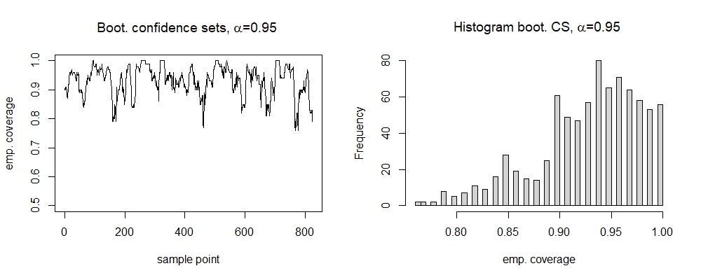
Figure 6: Empirical coverage and corresponding histogram for bootstrap confidence sets for curve $c_{1}$ and $J=10$, $J_{0}=7$

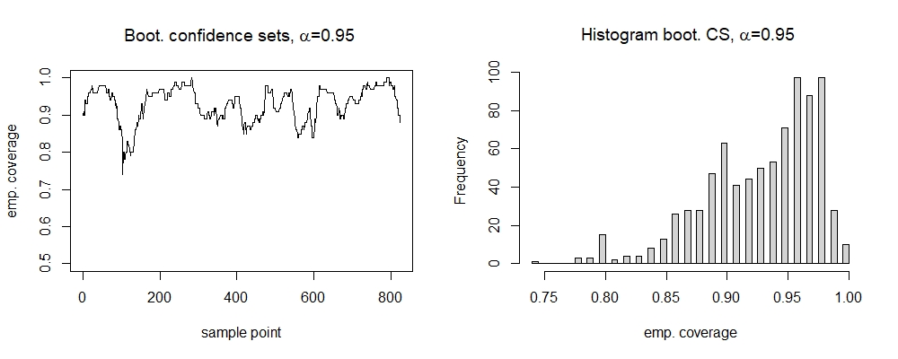
Figure 7: Empirical coverage and corresponding histogram for bootstrap confidence sets for curve $c_{2}$ and $J=10$, $J_{0}=5$

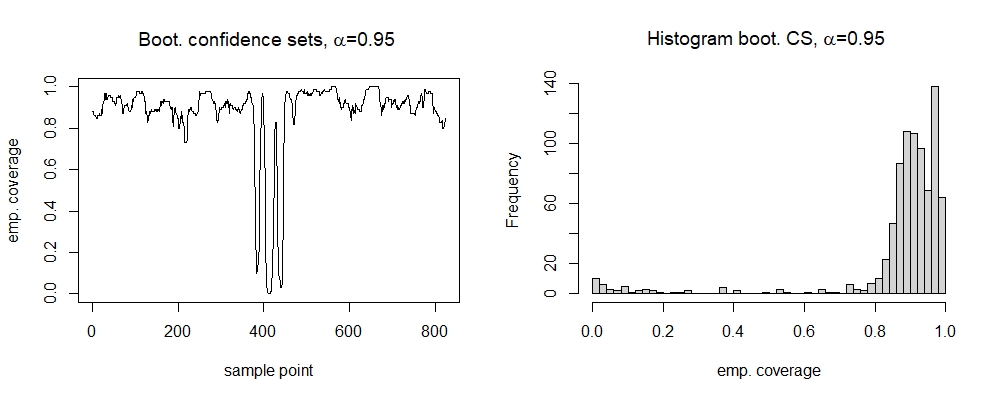
Figure 8: Empirical coverage and corresponding histogram for bootstrap confidence sets for curve $c_{3}$ and $J=10$, $J_{0}=6$

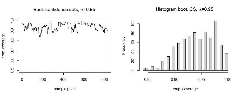
Figure 9: Empirical coverage and corresponding histogram for bootstrap confidence sets centred around the mean estimator for curve $c_{3}$ and $J=10$, $J_{0}=6$

Overall, we observe that for our bootstrap-based confidence sets not only our empirical coverages get close to the nominal ones on average (over all considered time points outside the boundaries) but also do we observe only a small proportion where this is not the case. This is likely to be the case due to the usual potential bias problem (as discussed above) which is inherent to any nonparametric curve estimation procedure - and not specific to our more challenging matrix-valued estimation problem. Quite satisfactorily, we also observe that the volumes of our bootstrap-based confidence sets are (on average) up to two orders of magnitude smaller than those that are given by the asymptotic approach. Recall that asymptotic confidence sets are known to be most often too conservative, which is also the reason for their empirical coverages observed here to be very close to $1$ (as already mentioned previously below equation (LABEL:E:ConfidenceSetLinearEstimator)).

7 Conclusions

In this paper we have been proposing two constructions of (pointwise) confidence sets for the (linear) wavelet estimator of SPD-matrix valued curves. Whereas mean-square consistency of our estimator on a Riemannian manifold, constructed via Average Interpolation wavelet schemes, is known to hold since the work by Chau and von Sachs [2021a], no such result on statistical inference has been existing before. In the first place, we have proven a Central Limit Theorem to hold for our linear wavelet estimator, which enables us to propose asymptotic confidence regions. These turned out to be rather conservative, as it is usually the case in nonparametric curve estimation problems, and in particular for curves living on curved, non-Euclidean manifolds. To circumvent this, we developed (wild) bootstrap confidence schemes which we showed to be theoretically valid, and empirically very satisfying: simulation studies confirmed these second sets to be far less conservative while keeping the nominal level.

Quite naturally, the question arises about inference for the non-linear version of our wavelet estimator, as proposed again by Chau and von Sachs [2021a], based on trace-thresholding of the matrix-valued empirical wavelet coefficients. Constructing confidence sets for this type of non-linear estimator is already a non-trivial task in the classical Euclidean set-up of first-generation wavelets for scalar curves, the related literature is sparse (e.g., Chau and von Sachs [2016], using Robins and Van Der Vaart [2006]). So although we believe that our approach based on the bootstrap sets can be successfully applied to the threshold wavelet estimator, we decided to leave this and further investigations on this question for future work. Note, however, that as a first theoretical step into this direction, we were able to derive a Central Limit Theorem, analogous to our Theorem 4.2, for the (whitened) empirical wavelet coefficients (3.10).

For the construction of our wavelet estimators, we used the log-Euclidean metric, which seems nicely taylored to the problem of denoising curves of SPD-matrix values. The log-Euclidean metric is among the computationally easiest constructions of Riemannian metrics for the space of positive symmetric matrices, replacing Euclidean distances by ones that are appropriate for this curved manifold. Moreover, our used metric enjoys important properties such as invariance with respect to unitarian congruent transformations. This implies in particular permutation-equivariant estimators of covariance matrices of multivariate or time series data (which is not the case for the often used Cholesky approach). Finally, and importantly for the constructions of correct confidence regions, this metric avoids any undesirable swelling effect: any element of the given confidence region remains a positive-definite symmetric matrix. Future work could be interesting in order to study whether our treated programme for inference could be developed for other matrix-valued objects, such as curves of positive semi-definite matrices.

Acknowledgements. Johannes Krebs gratefully acknowledges the support of the Deutsche Forschungsgemeinschaft (grants KR-4977/1-1, KR-4977/2-1) and the hospitality of ISBA/LIDAM (UCLouvain).

Supplement

8 Technical details on Section 3

8.1 Details on the AI refinement scheme of Section 3.2

Intrinsic polynomial interpolation. The fundamental tool for interpolation is Neville’s algorithm (Ma and Fu [2012], chapter 9.2) which can immediately be applied to our setting in the log-Euclidean metric. We only briefly sketch the nature of this interpolation scheme, more illustrations can be found in, again, Chau and von Sachs [2021a]. For given tupels $(x_{0},P_{0}),\ldots,(x_{n},P_{n})\in\mathbb{R}\times Sym^{+}(d)$ with $x_{i}<x_{i+1}$, let $p_{i,i}(x)=P_{i}$ for $x\in\mathbb{R}$ and $i=0,\ldots,n$. Now iteratively define

$$\begin{split}p_{i,j}(x)&=\mathrm{Exp}_{p_{i,j-1}(x)}\left(\frac{x-x_{i}}{x_{j}-x_{i}}\mathrm{Log}_{p_{i,j-1}(x)}(p_{i+1,j(x)})\right)\\ &=\exp\left\{\frac{x_{j}-x}{x_{j}-x_{i}}\log(p_{i,j-1}(x))+\frac{x-x_{i}}{x_{j}-x_{i}}\log(p_{i+1,j}(x))\right\},\end{split}$$ (8.1)

$0\leq i<j\leq n$, $x\in\mathbb{R}$. At the final iteration $p_{0,n}\colon\mathbb{R}\to Sym^{+}(d)$ is the intrinsic polynomial (of degree $n$) interpolating $P_{0},\ldots,P_{n}$ at $x_{0},\ldots,x_{n}$.

Derivation of (3.2):

$$\mathrm{Mean}(\rho;(k-L)2^{-j},(2k+1)2^{-(j+1)})$$

$$= \exp\left\{\frac{1}{(2L+1)2^{-(j+1)}}\left(\int_{(k-L)2^{-j}}^{k2^{-j}}\log(\rho(t))\,\mathrm{d}t+\int_{k2^{-j}}^{(2k+1)2^{-(j+1)}}\log(\rho(t))\,\mathrm{d}t\right)\right\}$$

$$= \exp\Bigg{\{}\frac{L2^{-j}}{(2L+1)2^{-(j+1)}}\log\circ\exp\left\{\frac{1}{L2^{-j}}\int_{(k-L)2^{-j}}^{k2^{-j}}\log(\rho(t))\,\mathrm{d}t\right\}$$

$$+\frac{1}{2L+1}\log\circ\exp\left\{\frac{1}{2^{-(j+1)}}\int_{k2^{-j}}^{(2k+1)2^{-(j+1)}}\log(\rho(t))\,\mathrm{d}t\right\}\Bigg{\}}$$

$$= \exp\left\{\frac{2L}{2L+1}\log(\mathrm{Mean}(\rho;(k-L)2^{-j},k2^{-j}))+\frac{1}{2L+1}\log(\widetilde{M}_{j+1,2k})\right\}$$

$$= \gamma\left(\frac{1}{2L+1};\overline{M}_{j,L},\widetilde{M}_{j+1,2k}\right).$$

Derivation of (3.3): Substituting the intrinsic interpolation polynomial into (3.2) we have

$$\pi((2k+1)2^{-(j+1)})=\exp\left\{\frac{2L}{2L+1}\log(\overline{M}_{j,L})+\frac{1}{2L+1}\log(\widetilde{M}_{j+1,2k})\right\}$$

which can be rearranged as

$$\gamma(-2L;\pi((2k+1)2^{-(j+1)}),\overline{M}_{j,L})$$

$$= \exp\left\{(2L+1)\log(\pi((2k+1)2^{-(j+1)})-2L\log(\overline{M}_{j,L}))\right\}$$

$$= \widetilde{M}_{j+1,2k}.$$

Details on Equations (3.5) and (3.6).

First, using (8.1), we can write out the first few iterations explicitly as follows:

$$p_{i-1,i}(x) =\exp\left\{\log(P_{i-1})+\frac{x-x_{i-1}}{x_{i}-x_{i-1}}\Big{(}\log(P_{i})-\log(P_{i-1})\Big{)}\right\},\quad$$

for $i\in\{1,\ldots,n\}$ and

$$\begin{split}&p_{i-2,i}(x)=\exp\Bigg{\{}\log(P_{i-2})+\Big{(}\frac{x-x_{i-2}}{x_{i-1}-x_{i-2}}-\frac{x-x_{i-2}}{x_{i}-x_{i-2}}\cdot\frac{x-x_{i-2}}{x_{i-1}-x_{i-2}}\\ &\qquad\qquad\qquad\qquad+\frac{x-x_{i-2}}{x_{i}-x_{i-2}}\Big{)}\Big{(}\log(P_{i-1})-\log(P_{i-2})\Big{)}\\ &\qquad\qquad\qquad\qquad+\frac{x-x_{i-2}}{x_{i}-x_{i-2}}\cdot\frac{x-x_{i-1}}{x_{i}-x_{i-1}}\Big{(}\log(P_{i})-\log(P_{i-1})\Big{)}\Bigg{\}},\end{split}$$ (8.2)

for $i\in\{2,\ldots,n\}$.

Next, denote $\widehat{M}((2k+1)2^{j})$ the intrinsic polynomial interpolating the points $(k2^{-(j-1)},\overline{M}_{j-1,1})$, $((k+1)2^{-(j-1)},\overline{M}_{j-1,2})$ and $((k+2)2^{-(j-1)},\overline{M}_{j-1,3})$. Evoking the explicit formula for $p_{0,2}$ in (LABEL:E:IntrinsicPolynomialInterpolationP02), we get

$$\widehat{M}((2k+1)2^{j})$$

$$= \exp\Bigg{\{}\log(\overline{M}_{j-1,1})+\left(\frac{1}{2}-\frac{1}{4}\cdot\frac{1}{2}+\frac{1}{4}\right)\Big{(}\log(\overline{M}_{j-1,2})-\log(\overline{M}_{j-1,1})\Big{)}$$

$$\quad\qquad-\frac{1}{4}\cdot\frac{1}{2}\Big{(}\log(\overline{M}_{j-1,3})-\log(\overline{M}_{j-1,2})\Big{)}\Bigg{\}}$$

$$= \exp\left\{\frac{17}{24}\log(M_{j-1,k-1})+\frac{1}{3}\log(M_{j-1,k})-\frac{1}{24}\log(M_{j-1,k+1})\right\}.$$

Therefore,

$$\widetilde{M}_{j,2k} =\exp\left\{3\log(\widehat{M}((2k+1)2^{j}))-2\log(\overline{M}_{j-1,1})\right\}$$

$$=\exp\left\{\frac{1}{8}\log(M_{j-1,k-1})+\log(M_{j-1,k})-\frac{1}{8}\log(M_{j-1,k+1})\right\}$$

as well as

$$\widetilde{M}_{j,2k+1} =\exp\left\{2\log(M_{j-1,k})-\log(\widetilde{M}_{j,2k})\right\}$$

$$=\exp\left\{-\frac{1}{8}\log(M_{j-1,k-1})+\log(M_{j-1,k})+\frac{1}{8}\log(M_{j-1,k+1})\right\}.$$

∎

8.2 Fast prediction

The operation $(\cdot)_{\diagdown d}$ commutes with multiplication.

Lemma 8.1.

Let $A\in\mathbb{R}^{m\times n}$ and $B\in\mathbb{R}^{n\times p}$ and $d\in\mathbb{N}_{+}$. Then $(AB)_{\diagdown d}=A_{\diagdown d}B_{\diagdown d}$. In addition, if $A$ is non singular, then $(A_{\diagdown d})^{-1}=(A^{-1})_{\diagdown d}$.

Proof.

Using the multiplication rules for block matrices, we have

$$A_{\diagdown d}B_{\diagdown d} =\Big{(}\Big{(}\sum_{k=1}^{m}(a_{i,k}I_{d})(b_{k,j}I_{d})\Big{)}_{i,j}\Big{)}_{i,j}=\Big{(}\Big{(}\sum_{k=1}^{m}a_{i,k}b_{k,j}I_{d}\Big{)}_{i,j}\Big{)}_{i,j}$$

$$=\Big{[}\Big{(}\Big{(}\sum_{k=1}^{m}a_{i,k}b_{k,j}\Big{)}_{i,j}\Big{)}_{i,j}\Big{]}_{\diagdown d}=(AB)_{\diagdown d}.$$

Moreover, if $A^{-1}$ exists, then

$$I_{nd}=(I_{n})_{\diagdown d}=(AA^{-1})_{\diagdown d}=A_{\diagdown d}(A^{-1})_{\diagdown d},$$

i.e., $(A^{-1})_{\diagdown d}$ is the inverse of $A_{\diagdown d}$. ∎

This lemma implies the following structural result regarding the characteristic polynomial of a square matrix.

Corollary 8.2.

Let $A\in\mathbb{R}^{n\times n}$ with Jordan decomposition $A=SJS^{-1}$ and characteristic polynomial $\chi_{A}(\lambda)=det(A-\lambda I_{n})$. Then

$$A_{\diagdown d}=S_{\diagdown d}J_{\diagdown d}(S_{\diagdown d})^{-1}$$

and $\chi_{A_{\diagdown d}}(\lambda)=(\chi_{A}(\lambda))^{d}$.

Proof.

First using Lemma 8.1, we see

$$A_{\diagdown d}=(SJS^{-1})_{\diagdown d}=S_{\diagdown d}J_{\diagdown d}(S^{-1})_{\diagdown d}=S_{\diagdown d}J_{\diagdown d}(S_{\diagdown d})^{-1}.$$

Consequently, using Lemma 8.1 another time, the characteristic polynomial of $A_{\diagdown d}$ satisfies

$$\chi_{A_{\diagdown d}}(\lambda) =\det((SJS^{-1})_{\diagdown d}-\lambda I_{nd})=\det(S_{\diagdown d}(J_{\diagdown d}-\lambda I_{nd})(S_{\diagdown d})^{-1})$$

$$=\det(J_{\diagdown d}-\lambda I_{nd})=\det(J-\lambda I_{n})^{d}=\chi_{A}(\lambda)^{d}.$$

This completes the proof. ∎

Proof of Lemma 3.2.

The assertion obviously holds for $m=1$.
$m\to m+1:$ Let $p\in\{0,\ldots,2^{m+1}-1\}$. Suppose $p$ is even. Then $p=2q$ for a $q\in\{0,\ldots,2^{m}-1\}$. By (3.13) we get

$$\begin{bmatrix}\log\widetilde{M}_{j+m+1,2^{m+1}k-2L+p}\\ \vdots\\ \log\widetilde{M}_{j+m+1,2^{m+1}k+2L+p}\end{bmatrix} =\begin{bmatrix}\log\widetilde{M}_{j+m+1,2(2^{m}k+q)-2L}\\ \vdots\\ \log\widetilde{M}_{j+m+1,2(2^{m}k+q)+2L}\end{bmatrix}$$

$$=(E_{N})_{\diagdown d}\begin{bmatrix}\log\widetilde{M}_{j+m,2^{m}k+q-2L}\\ \vdots\\ \log\widetilde{M}_{j+m,2^{m}k+q+2L}\end{bmatrix}$$

$$=(E_{N})_{\diagdown d}\cdot X_{m}\cdot\ldots\cdot X_{1}\begin{bmatrix}\log M_{j,k-2L}\\ \vdots\\ \log M_{j,k+2L}\end{bmatrix}.$$

Suppose $p$ is odd, than $p=2q+1$ for $q\in\{0,\ldots,2^{m}-1\}$. Using (3.14) a similar calculation yields the assertion. ∎

9 Technical details on wavelet regression in Section 4

Lemma 9.1.

Let $u=k2^{-J}$ be a dyadic rational in $[0,1]$, then

$$\|{\cal C}(u)\|_{\cal L}\leq\mathbb{E}[\|\log M_{J,k,n}\|_{F}^{2}].$$

In particular, $\sup_{u\in[0,1]}\|{\cal C}(u)\|_{\cal L}\leq\sup\mathbb{E}[\|\log M_{J,k,n}\|_{F}^{2}]$, where the supremum on the right-hand side is taken over all dyadic rationals.

Proof.

Let $\varepsilon>0$. For each $u\in[0,1]$, there is an $A_{u}\in Sym(d)$, $\|A_{u}\|_{F}=1$, such that

$$\|{\cal C}(u)\|_{\cal L}-\varepsilon\leq\|{\cal C}(u)A_{u}\|_{F}=\langle{\cal C}(u)A_{u},{\cal C}(u)A_{u}\rangle^{1/2}.$$

Let $u=k2^{-J}$ be a dyadic rational for $n=2^{J}$. The square of the right-hand side of the last inequality equals by definition

$$\mathrm{Cov}(\langle{\cal C}(u)A_{u},\log M_{J,k,n}\rangle,\langle A_{u},\log M_{J,k,n}\rangle)$$

$$\leq\mathrm{Var}(\langle{\cal C}(u)A_{u},\log M_{J,k,n}\rangle)^{1/2}\mathrm{Var}(\langle A_{u},\log M_{J,k,n}\rangle)^{1/2}.$$

Obviously, $\mathrm{Var}(\langle A_{u},\log M_{J,k,n}\rangle)\leq\mathbb{E}[\|\log M_{J,k,n}\|_{F}^{2}]$. Also,

$$\mathrm{Var}(\langle{\cal C}(u)A_{u},\log M_{J,k,n}\rangle)$$

$$\leq\mathbb{E}[\langle{\cal C}(u)A_{u},\log M_{J,k,n}\rangle^{2}]$$

$$=\mathbb{E}[\mathrm{Cov}(\langle A_{u},\log M_{J,k,n}\rangle,\langle B,\log M_{J,k,n}\rangle)^{2}|_{B=\log M_{J,k,n}}]$$

$$\leq\mathbb{E}[\mathrm{Var}(\langle A_{u},\log M_{J,k,n}\rangle)\ \mathrm{Var}(\langle B,\log M_{J,k,n}\rangle)|_{B=\log M_{J,k,n}}]$$

$$\leq\mathrm{Var}(\langle A_{u},\log M_{J,k,n}\rangle)\ \mathbb{E}[\mathbb{E}[\langle B,\log M_{J,k,n}\rangle^{2}]|_{B=\log M_{J,k,n}}]$$

$$\leq\mathbb{E}[\|\log M_{J,k,n}\|_{F}^{2}]\ \mathbb{E}[\mathbb{E}[\|B\|_{F}^{2}\|\log M_{J,k,n}\|_{F}^{2}]|_{B=\log M_{J,k,n}}]$$

$$=\mathbb{E}[\|\log M_{J,k,n}\|_{F}^{2}]^{3}.$$

Thus, $\|{\cal C}(u)A_{u}\|_{F}\leq\mathbb{E}[\|\log M_{J,k,n}\|_{F}^{2}]$.

The amendment follows from the càdlàg property of ${\cal C}$. ∎

In order to prove the asymptotic normality, we rely on Lyapunov’s condition.

Theorem 9.2 (Lyapunov condition).

Let $(\xi_{n,i})_{i=1}^{\ell_{n}}$ be a sequence of independent real-valued random variables for each $n\in\mathbb{N}$ such that $\ell_{n}\leq cn$ for some $c>0$. Assume $\lim_{n\to\infty}n^{-1}\sum_{i=1}^{\ell_{n}}Var(\xi_{n,i})=\sigma^{2}<\infty$ and $\sup_{n}\sup_{i}\mathbb{E}[|\xi_{n,i}|^{2+\delta}]<\infty$ for some $\delta>0$. Then $n^{-1/2}\sum_{i=1}^{\ell_{n}}(\xi_{n,i}-\mathbb{E}[\xi_{n,i}])\Rightarrow{\cal N}(0,\sigma^{2})$ as $n\to\infty$.

Proof of Proposition 4.2.

To keep the notation simple, we omit the dependence of the quantities $J,j,J_{0},k$ on $n$. We split the proof in two parts, the first part covering the statement for the fixed dyadic number $k2^{-j}$, the second the statement for $k2^{-j}\to x$.

(a) We rely on the Cramér-Wold-device. Let $A\in Sym(d)$ be arbitrary but fixed. In the first step, we derive the limiting expression of the covariance operator. A representation of $\log M_{j,k,n}$ in terms of the $\log M_{J,u,n}$ follows from the midpoint pyramid algorithm because

$$\log M_{j,k,n}=2^{-(J-j)}\sum_{u=0}^{2^{(J-j)}-1}\log M_{J,u+k2^{(J-j)},n}.$$ (9.1)

In particular, using the independence of the $(M_{J,k,n})_{k}$, we obtain from (9.1)

$$2^{-j}n\ \mathrm{Var}(\langle A,\log M_{j,k,n}\rangle) =2^{-(J-j)}\sum_{u=0}^{2^{(J-j)}-1}\mathrm{Var}(\langle A,\log M_{J,u+k2^{(J-j)},n}\rangle)$$

$$=2^{-(J-j)}\sum_{u=0}^{2^{(J-j)}-1}\langle A,{\cal C}(u2^{-J}+k2^{-j})A\rangle,$$ (9.2)

where ${\cal C}(u2^{-J}+k2^{-j})$ is the covariance operator of $\log M_{J,u+k2^{(J-j)},n}$. Using the convergence result from (LABEL:E:ConvergenceCovOp), the right-hand side of (9.2) converges to

$$c^{*}=2^{j}\int_{k2^{-j}}^{(k+1)2^{-j}}\langle A,{\cal C}(u)A\rangle\mathop{}\!\mathrm{d}u>0.$$

The Lyapunov condition from Theorem 9.2 can now be established with the help of this last convergence result and the uniform bounded moments condition of the curve from (4.1). The latter implies

$$\begin{split}\mathbb{E}[|\langle A,\log M_{J,u,n}\rangle|^{2+\delta}]&\leq\|A\|_{F}^{2+\delta}\ \sup\mathbb{E}[\|\log M_{J,u,n}\|_{F}^{2+\delta}]<\infty,\end{split}$$ (9.3)

where the last supremum is taken over $u\in\{0,\ldots,2^{J}-1\}$ and $J\in\mathbb{N}_{+}$. So, the requirements of Theorem 9.2 for the array $(\langle A,\log M_{J,u+k2^{J-j},n}\rangle)_{u}$ are satisfied and $2^{-j/2}n^{1/2}(\log M_{j,k,n}-\mathbb{E}[\log M_{j,k,n}])\Rightarrow{\cal N}(0,c^{*})$ as $n\to\infty$. This shows (a).

(b) Let $k2^{-J_{0}}\to x$. We verify the limit of the variance using (9.2). We have

$$|\langle A,{\cal C}(k2^{-J_{0}}+u2^{-J})A\rangle-\langle A,{\cal C}(x)A\rangle|\leq\|A\|_{F}^{2}\ \|{\cal C}(k2^{-J_{0}}+u2^{-J})-{\cal C}(x)\|_{\cal L}.$$

Plainly, $|k2^{-J_{0}}+u2^{-J}-x|\leq|k2^{-J_{0}}-x|+2^{-J_{0}}\rightarrow 0$. Using the continuity of $\cal C$ in the point $x$,

$$\lim_{n\to\infty}2^{-J_{0}}n\ \mathrm{Var}(\langle A,\log M_{J_{0},k,n}\rangle)=\langle A,{\cal C}(x)A\rangle>0.$$

The Lyaponov condition for the sequence $(J_{0,n},k_{n})_{n}$ can be verified in a similar spirit as in (a). This completes the proof. ∎

For proving Theorem 4.4, in order to study the AI wavelet estimator at a specific point $x\in[0,1]$, we introduce some terminology regarding the representation of dyadic numbers in the unit interval. Let $x\in[0,1]$ have the dyadic representation $(d_{0},d_{1},\ldots)$, that is $x=\sum_{i=0}^{\infty}2^{-i}d_{i}.$ We agree to choose the shortened form for dyadic rationals, e.g., we choose the representation $(d_{0},d_{1},\ldots,d_{j},1,0,0,\ldots,)$ for the number $x=\sum_{i=0}^{j}2^{-i}d_{i}+2^{j+1}$. (We could use the representation $(d_{0},d_{1},\ldots,d_{j},0,1,1,\ldots)$ instead, this does not change the arguments much).

Define for a scale $j\in\mathbb{N}_{+}$ the dyadic approximation of $x$ by the first $j$ entries $x^{(j)}=(d_{0},d_{1},\ldots,d_{j})$. This means, the dyadic rational $x^{(j)}$ is a ratio of the form $k^{(j)}2^{-j}$, where

$$k^{(j)} =\sum_{i=0}^{j}2^{i}d_{j-i}=2^{0}d_{j}+2d_{j-1}+\ldots+2^{j-j^{\prime}-1}d_{j^{\prime}+1}+2^{j-j^{\prime}}\sum_{i=0}^{j^{\prime}}2^{i}d_{j^{\prime}-i}$$

$$=2^{0}d_{j}+2d_{j-1}+\ldots+2^{j-j^{\prime}-1}d_{j^{\prime}+1}+2^{j-j^{\prime}}k^{\prime}_{j,j^{\prime}},$$ (9.4)

for a smaller scale $j^{\prime}\leq j$ and the residual integer $k^{\prime}_{j,j^{\prime}}=\sum_{i=0}^{j^{\prime}}2^{i}d_{j^{\prime}-i}$.

Proof of Theorem 4.4.

To keep the notation simple, we omit the dependence of the quantities $J,J_{0},k$ on $n$. Let $N+1\leq k\leq 2^{J}-1-N-1$, so that $(J,k)$ is sufficiently far away from the boundary. Since $(J,k)\to x\in(0,1)$ this is the case if $n$ is large enough. Let $\ell=J-J_{0}\to\infty$ for a base level $J_{0}$ which tends to $\infty$. Substituting $J$ for $j$ and $J_{0}$ for $j^{\prime}$ in (9.4) we have the following representation for the integer $k=k_{n}$

$$k=2^{0}d_{J}+2^{1}d_{J-1}+\ldots+2^{\ell-1}d_{J_{0}+1}+2^{\ell}k_{0},$$ (9.5)

where $k_{0}=k^{\prime}_{J,J^{\prime}}$ is the approximating integer on the scale $J_{0}$.

Using the matrices $E_{N},O_{N}$ from equations ($E_{N}$) and ($O_{N}$) and the corresponding transformation matrices $(E_{N})_{\diagdown d},(O_{N})_{\diagdown d}$, we obtain the representation of the wavelet estimator w.r.t. the base level $J_{0}$

$$\begin{split}&\begin{pmatrix}\log\widehat{M}_{J,k-N-1,n}\\ \vdots\\ \log\widehat{M}_{J,k+N+1,n}\end{pmatrix}=\Big{[}(E_{N}\mathds{1}\{d_{J}=0\}+O_{N}\mathds{1}\{d_{J}=1\})\cdot\ldots\\ &\quad\ldots\cdot(E_{N}\mathds{1}\{d_{J_{0}+1}=0\}+O_{N}\mathds{1}\{d_{J_{0}+1}=1\})\Big{]}_{\diagdown d}\begin{pmatrix}\log M_{J_{0},k_{0}-N-1,n}\\ \vdots\\ \log M_{J_{0},k_{0}+N+1,n}\end{pmatrix}.\end{split}$$ (9.6)

In particular, for $i\in[-(N+1)..(N+1)]$, using the representation from (9.1)

$$\begin{split}\log\widehat{M}_{J,k+i,n}&=\sum_{v=-(N+1)}^{N+1}\alpha_{v}\log M_{J_{0},k_{0}+v,n}\\ &=\sum_{v=-(N+1)}^{N+1}\alpha_{v}2^{-\ell}\sum_{u=0}^{2^{\ell}-1}\log M_{J,u+(k_{0}+v)2^{\ell},n}\end{split}$$ (9.7)

for certain coefficients $\alpha_{v}$, which sum to 1 and depend on $J_{0}$ and $J$. So, for each coefficient $\alpha_{v}$, there is a corresponding finite matrix product consisting of $E_{N}$ and $O_{N}$. Thus, the $\alpha_{v}$ depend on $n$, we omit this dependence in the notation in the following. Note that this implies immediately that $\sum_{v}\alpha_{v}^{2}\geq 1/(2N+3)$ uniformly which follows from minimization problem

$$\min_{w_{1},\ldots,w_{L},\lambda}\ \Big{[}\sum_{v}w_{v}^{2}+\lambda(\sum_{v}w_{v}-1)\Big{]}.$$

Consider the variance of $\log{\widehat{M}}_{J,k,n}$. Then we find for a matrix $0\neq A\in Sym(d)$

$$\begin{split}&Var(2^{\ell/2}\langle A,\log{\widehat{M}}_{J,k,n}\rangle)\\ &=\sum_{v=-(N+1)}^{N+1}\alpha_{v}^{2}\sum_{u=0}^{2^{\ell}-1}2^{-\ell}\langle A,{\cal C}(2^{-J}(u+(k_{0}+v)2^{\ell}))A\rangle.\end{split}$$ (9.8)

We can use the convergence of $x^{(J_{n})}$ to $x$ and continuity of the covariance operator in $x$ to obtain upper and lower bounds on (LABEL:E:NormalityLinEst3).

Once more, $|2^{-J}(u+(k_{0}+v)2^{\ell})-x|\leq|k_{0}2^{-J_{0}}-x|+2^{-J_{0}}+(N+1)2^{-(J-J_{0})}$, which tends to 0 as $n\to\infty$. Hence,

$$\liminf_{n\to\infty}Var(2^{\ell/2}\langle A,\log{\widehat{M}}_{J,k,n}\rangle)=\langle A,{\cal C}(x)A\rangle\ \liminf_{n\to\infty}\ \Big{(}\sum_{v=-(N+1)}^{N+1}\alpha_{v}^{2}\Big{)}$$

$$\geq(2N+3)^{-1}\langle A,{\cal C}(x)A\rangle>0,$$ (9.9)

because $A\neq 0$. With the same reasoning, an upper bound is given by

$$\limsup_{n\to\infty}Var(2^{\ell/2}\langle A,\log{\widehat{M}}_{J,k,n}\rangle)=\langle A,{\cal C}(x)A\rangle\ \limsup_{n\to\infty}\ \Big{(}\sum_{v=-(N+1)}^{N+1}\alpha_{v}^{2}\Big{)}$$

$$\leq\|{\cal C}(x)\|_{\cal L}\|A\|_{F}^{2}\ \limsup_{n\to\infty}\ \Big{(}\sum_{v=-(N+1)d}^{(N+1)d}\alpha_{v}^{2}\Big{)}.$$ (9.10)

So, the left-hand side of (9.9) and (9.10) agree if and only if $\sum_{v=-(N+1)d}^{(N+1)d}\alpha_{v}^{2}$ converges to a number in $\mathbb{R}_{+}$ as $n\to\infty$.

If $x=2^{-j}k$ is a dyadic rational, then the iteration in (LABEL:E:NormalityLinEst2) is ultimately carried out with the matrix $E_{N}$ only because $J\geq J_{0}>j$ if $n$ is sufficiently large and $d_{J}=...=d_{J_{0}+1}=0$ is the representation of $x$. In particular, in this case the limit

$$\lim_{n\to\infty}\sum_{v=-(N+1)}^{N+1}\alpha_{v}^{2}=\sum_{v=-(N+1)}^{N+1}\lim_{n\to\infty}\alpha_{v}^{2}=\sum_{i=1}^{2N-1}(E_{N,\infty})^{2}_{N,i}$$ (9.11)

exists in $\mathbb{R}_{+}$ by the considerations which lead to (3.16). (Note that if we use the infinite representation for dyadic rationals, we multiply with $O_{N}$ instead.) Consequently, in this case

$$\lim_{n\to\infty}Var(2^{\ell/2}\langle A,\log{\widehat{M}}_{J,k,n}\rangle)=\Big{(}\sum_{i=1}^{2N-1}(E_{N,\infty})^{2}_{N,i}\Big{)}\ \langle A,{\cal C}(x)A\rangle\in\mathbb{R}_{+}.$$

This completes the proof. ∎

Proof of Proposition 4.5.

The result follows in a similar spirit as Theorem 4.4. Let $\delta>0$ such that the uniform bounded moments condition in (4.1) is satisfied for $2+\delta$. The Lyapunov condition for the normalized estimator

$$\begin{split}&Var(\langle A,\log\widehat{M}_{J,k,n}-\mathbb{E}[\log\widehat{M}_{J,k,n}]\rangle)^{-1/2}\cdot\langle A,\log\widehat{M}_{J,k,n}-\mathbb{E}[\log\widehat{M}_{J,k,n}]\rangle\end{split}$$ (9.12)

can be established with the representation from (9.7) and reads as follows

$$\frac{\sum_{v=-(N+1)}^{N+1}(|\alpha_{v}|\ 2^{-\ell})^{2+\delta}\sum_{u=0}^{2^{\ell}-1}\mathbb{E}[|\langle A,\log M_{J,u+(k_{0}+v)2^{\ell},n}-\mathbb{E}[\log M_{J,u+(k_{0}+v)2^{\ell},n}]\rangle|^{2+\delta}]}{\Big{(}\sum_{v=-(N+1)}^{N+1}\sum_{u=0}^{2^{\ell}-1}(\alpha_{v}2^{-\ell})^{2}\mathbb{E}[|\langle A,\log M_{J,u+(k_{0}+v)2^{\ell},n}-\mathbb{E}[\log M_{J,u+(k_{0}+v)2^{\ell},n}]\rangle|^{2}]\Big{)}^{(2+\delta)/2}}.$$

In order to give an upper bound on this term, we use the uniform bounded moments condition in (4.1), the lower bound $\sum_{v}\alpha_{v}^{2}\geq 1/(2N+3)$ as well as the upper bound

$$\limsup_{n\to\infty}\max_{-(N+1)\leq v\leq N+1}|\alpha_{v}| =\limsup_{J_{0}\to\infty}\lim_{J\to\infty}\max_{-(N+1)\leq v\leq N+1}|\alpha_{v}|$$

$$\leq\sup_{x\in[0,1]}\max_{i,j}~{}\Phi_{L}(x)_{i,j}<\infty,$$

where $\Phi_{L}(x)$ is the limit matrix in (3.16); notice that the entries of $\Phi_{L}(x)$ are uniformly bounded due to the Hölder continuity of the fundamental solution $\varphi_{L}$, cf. Donoho [1993].

Combining these estimates, the term in question is of order $2^{-\delta\ell/2}$. Hence, the Lyapunov condition is satisfied. ∎

10 Technical results on the wild bootstrap in Section 5

Proof of Theorem 5.2.

The proof is split in three parts. In the first part we study the limiting behavior of the conditional variance of the bootstrap estimator. In the second part, we verify then the Lindeberg condition. In the third part, we show the amendment. To facilitate the notation, we use the following abbreviations. Set $\ell\coloneqq J-J_{0}$. Let $A\in Sym(d)$ and define

$$\widehat{Z}_{u,n}=\langle A,\ \log\widehat{M}_{J^{*}_{0},J,2^{\ell}k+u,n}\rangle,\ Z_{u,n}=\langle A,\log M_{J,2^{\ell}k+u,n}\rangle,Z_{u}=\langle A,\log M_{J,2^{\ell}k+u}\rangle$$

for $u\in\{0,\ldots,2^{\ell}-1\}$. We choose $\delta,\gamma>0$ such that $p=\gamma(2+\delta)$, $\gamma\geq 2$ and such that $\delta$ is sufficiently small; see below for the admissible choices.

Part 1. The conditional variance of $\log M_{J_{0},k,n}^{boot}$ is

$$Var^{*}(2^{-\ell/2}\langle A,\log M_{J_{0},k,n}^{boot}\rangle) =2^{-\ell}\sum_{u=0}^{2^{\ell}-1}(\widehat{Z}_{u,n}-Z_{u,n})^{2}.$$

We split each summand in a main term and remainder terms as follows

$$\widehat{Z}_{u,n}-Z_{u,n}=(\widehat{Z}_{u,n}-\mathbb{E}[\widehat{Z}_{u,n}])+(\mathbb{E}[\widehat{Z}_{u,n}]-Z_{u})+(Z_{u}-Z_{u,n}).$$ (10.1)

We begin with the term $2^{-\ell}\sum_{u=0}^{2^{\ell}-1}(\widehat{Z}_{u,n}-\mathbb{E}[\widehat{Z}_{u,n}])^{2}$ on which we apply the following simple consequence of the Burkholder inequality; we state this consequence as a lemma:

Lemma 10.1.

Let $W_{1},\ldots,W_{n}$ be independent, real-valued, centered random variables such that $\max_{i}\mathbb{E}[|W_{i}|^{q}]^{1/q}\leq m$, for some $q\geq 2$ and an $m\in\mathbb{R}_{+}$. Then $\mathbb{E}[|\sum_{i}W_{i}|^{q}]\leq C_{q}^{q}\ m^{q}\ n^{q/2}$ for a certain $C_{q}\in\mathbb{R}_{+}$.

Proof of Lemma 10.1.

Using the Burkholder inequality, $\mathbb{E}[|W_{i}|^{q}]\leq C_{q}^{q}\mathbb{E}[(\sum_{i}W_{i}^{2})^{q/2}]$ for some $C_{q}\in\mathbb{R}_{+}$. As $q\geq 2$, we apply the Minkowski inequality to obtain the result. ∎

Utilizing (3.16), we find with Lemma 10.1 and the moment condition on $Z_{u,n}$ from (4.1) as well as the representation of the wavelet estimator from (9.7) that for each $\gamma,\varepsilon>0$

$$\mathbb{P}\Big{(}2^{-\ell}\sum_{u=0}^{2^{\ell}-1}(\widehat{Z}_{u,n}-\mathbb{E}[\widehat{Z}_{u,n}])^{2}\geq\varepsilon\Big{)}\leq\sum_{u=0}^{2^{\ell}-1}\mathbb{P}((\widehat{Z}_{u,n}-\mathbb{E}[\widehat{Z}_{u,n}])^{2}\geq\varepsilon)$$

$$\leq\varepsilon^{-\gamma}\ \sum_{u=0}^{2^{\ell}-1}\mathbb{E}[|\widehat{Z}_{u,n}-\mathbb{E}[\widehat{Z}_{u,n}]|^{2\gamma}]\leq C_{1}\varepsilon^{-\gamma}\ 2^{(J-J_{0})-(J-J_{0}^{*})\gamma},$$

for a constant $C_{1}$, which does not depend on $n$. (Note that in the first inequality, we can use this quite rough estimate because the $(\widehat{Z}_{u,n})_{u}$ are dependent.) So, provided $\delta>0$ is sufficiently small, $\sum_{n}2^{(J-J_{0})-(J-J_{0}^{*})p/(2+\delta)}<\infty$ and we can apply the Borel-Cantelli Lemma to conclude that the partial sum

$$2^{-\ell}\sum_{u=0}^{2^{\ell}-1}(\widehat{Z}_{u,n}-\mathbb{E}[\widehat{Z}_{u,n}])^{2}\to 0\quad a.s.,\quad n\to\infty.$$

Moreover, there is a constant $C_{2}\in\mathbb{R}_{+}$ (independent of $n$) such that

$$(\mathbb{E}[\widehat{Z}_{u,n}]-Z_{u})^{2}\leq C_{2}2^{-2NJ^{*}_{0}}$$

uniformly in $u\in\{0,\ldots,2^{\ell}-1\}$ by the approximation result from [Chau, 2018, Appendix A]. Thus, the deterministic sum $2^{-\ell}\sum_{u=0}^{2^{\ell}-1}(\mathbb{E}[\widehat{Z}_{u,n}]-Z_{u})^{2}$ converges to 0 as $n\to\infty$.

Finally, consider $2^{-\ell}\sum_{u=0}^{2^{\ell}-1}(Z_{u,n}-Z_{u})^{2}$, which has expectation

$$2^{-\ell}\sum_{u=0}^{2^{\ell}-1}\langle A,{\cal C}(2^{-J_{0}}k+2^{-J}u)A\rangle.$$

Hence, using Lemma 10.1 a second time, for each $\gamma>0$ there is a $C_{3}\in\mathbb{R}_{+}$ (independent of $n$) such that

$$\mathbb{P}\Big{(}2^{-\ell}\Big{|}\sum_{u=0}^{2^{\ell}-1}(Z_{u,n}-Z_{u})^{2}-\mathbb{E}[(Z_{u,n}-Z_{u})^{2}]\Big{|}\geq\varepsilon\Big{)}$$

$$\leq 2^{-\ell\gamma}\varepsilon^{-\gamma}\ \mathbb{E}\Big{[}\Big{|}\sum_{u=0}^{2^{\ell}-1}(Z_{u,n}-Z_{u})^{2}-\mathbb{E}[(Z_{u,n}-Z_{u})^{2}]\Big{|}^{\gamma}\Big{]}\leq C_{3}\varepsilon^{-\gamma}2^{-(J-J_{0})\gamma/2}.$$

Consequently, provided $\sum_{n}2^{-(J-J_{0})p/(2(2+\delta))}<\infty$, which is satisfied if we choose $\delta$ sufficiently small, we have

$$2^{-\ell}\sum_{u=0}^{2^{\ell}-1}(Z_{u,n}-Z_{u})^{2}-\mathbb{E}[(Z_{u,n}-Z_{u})^{2}]\to 0\quad a.s.\quad(n\to\infty).$$

Thus, using the convergence result of the covariance operator from (9.2)

$$2^{-\ell}\sum_{u=0}^{2^{\ell}-1}(Z_{u,n}-Z_{u})^{2}\to 2^{J_{0}}\int_{k2^{-J_{0}}}^{(k+1)2^{-J_{0}}}\langle A,{\cal C}(u)A\rangle\mathop{}\!\mathrm{d}{u}>0\quad a.s.$$

In particular, $Var^{*}(2^{-\ell/2}\langle A,\log M_{J_{0},k,n}^{boot}\rangle)/Var(2^{-\ell/2}\langle A,\log M_{J_{0},k,n}\rangle)\to 1$ with probability 1 as $n\to\infty$.

Consequently, we have

$$Var^{*}(2^{-\ell/2}\langle A,\log\widehat{M}_{J_{0},J,k,n}^{boot}\rangle)/Var(2^{-\ell/2}\langle A,\log\widehat{M}_{J,k,n}\rangle)\to 1$$

with probability 1 as $n\to\infty$.

Part 2. For simplicity, we verify the Lindeberg condition only for $2^{\ell/2}\log M^{boot}_{J_{0},k,n}=2^{-\ell/2}\sum_{u=0}^{2^{\ell}-1}\log M^{boot}_{J,u+2^{\ell}k,n}$; the actual verification for the wavelet estimator works in the same fashion but involves a little more notation.

Note that $\mathbb{E}^{*}[\log M^{boot}_{J,k,n}]=\log\widehat{M}_{J^{*}_{0},J,k,n}$ and that $\log M^{boot}_{J,k,n}-\log\widehat{M}_{J^{*}_{0},J,k,n}=\varepsilon^{boot}_{J,k,n}$. Moreover, as the conditional variance of this random variable converges $a.s.$ by the previous arguments, it is sufficient to prove the following Lindeberg condition in order to verify the conditional CLT

$$L^{boot}_{n}(\mu) =\sum_{u=0}^{2^{\ell}-1}\mathbb{E}^{*}\Big{[}|2^{-\ell/2}\langle A,\varepsilon^{boot}_{J,u+2^{\ell}k,n}\rangle|^{2}\mathds{1}\{|2^{-\ell/2}\langle A,\varepsilon^{boot}_{J,u+2^{\ell}k,n}\rangle|>\mu\}\Big{]}\to 0$$

for each $\mu>0$ with probability 1. Let $\delta>0$, then we have

$$L^{boot}_{n}(\mu)\leq\mu^{-\delta}\ \mathbb{E}^{*}[|V_{0,0,n}|^{2+\delta}]\ 2^{-\ell(1+\delta/2)}\sum_{u=0}^{2^{\ell}-1}|\langle A,\hat{\varepsilon}^{*}_{J,u+2^{\ell}k,n}\rangle|^{2+\delta}.$$

Since $\langle A,\hat{\varepsilon}^{*}_{J,u+2^{\ell}k,n}\rangle=\widehat{Z}_{u,n}-Z_{u,n}$, we rely on the same decomposition as in (10.1). It is a routine to show similarly as in the first part of the proof but this time with the exponent $2+\delta$ instead of 2 that

$$2^{-\ell}\sum_{u=0}^{2^{\ell}-1}|\widehat{Z}_{u,n}-\mathbb{E}[\widehat{Z}_{u,n}]|^{2+\delta}=o_{a.s.}(1)$$

for the choices of $\delta$ and $\gamma$. Furthermore, for the choices of $\delta$ and $\gamma$,

$$2^{-\ell}\sum_{u=0}^{2^{\ell}-1}|\mathbb{E}[\widehat{Z}_{u,n}]-Z_{u}|^{2+\delta}=o(1)\text{ and }2^{-\ell}\sum_{u=0}^{2^{\ell}-1}|Z_{u,n}-Z_{u}|^{2+\delta}=O_{a.s.}(1).$$

Using the monotonicity of $L^{boot}_{n}(\mu)$ in $\mu$, this shows then that $L^{boot}_{n}(\mu)\to 0$ for $n\to\infty$ for all $\mu>0$ with probability 1.

Part 3. The convergence in the Kolmogorov distance follows from a standard argument as the limiting Gaussian distribution of $\mathfrak{M}_{J,k,n}$ and $\mathfrak{M}_{J,k,n}^{boot}$ has a continuous density on $Sym(d)\cong\mathbb{R}^{(d+1)d/2}$. Let $\cal N$ be a random variable having this Gaussian distribution and let $\mu>0$. Let $\Gamma$ be a finite grid on $Sym(d)$ with minimal element $\underline{x}$ and maximal element $\overline{x}$, i.e., $\underline{x}\leq x\leq\overline{x}$ for all $x\in\Gamma$. (Here $x\leq y$ for $x,y\in Sym(d)$ if for each position $(i,j)$, $x_{i,j}\leq y_{i,j}$.) For $x\in Sym(d)$ with $\underline{x}\leq x\leq\overline{x}$, denote $\lfloor x\rfloor$ (resp. $\lceil x\rceil$) the elements in $\Gamma$ which are closest to $x$ in the maximum-norm and satisfy $\lfloor x\rfloor\leq x$ (resp. $x\leq\lceil x\rceil$). We choose $\Gamma$ sufficiently dense in the sense that $\mathbb{P}({\cal N}\leq\underline{x})\leq\mu$, $1-\mathbb{P}({\cal N}\leq\overline{x})\leq\mu$ and $\mathbb{P}({\cal N}\leq\lceil x\rceil)-\mathbb{P}({\cal N}\leq\lfloor x\rfloor)\leq\mu$ for $\underline{x}\leq x\leq\overline{x}$.

Next, choose $N\in\mathbb{N}$ large enough such that $|\mathbb{P}(\mathfrak{M}_{J,k,n}\leq x)-\mathbb{P}({\cal N}\leq x)|\leq\mu$ and $|\mathbb{P}(\mathfrak{M}_{J,k,n}^{boot}\leq x)-\mathbb{P}({\cal N}\leq x)|\leq\mu$ for all $x\in\Gamma$ for all $n\geq N$.

Then $|\mathbb{P}(\mathfrak{M}_{J,k,n}\leq x)-\mathbb{P}(\mathfrak{M}_{J,k,n}^{boot}\leq x)|\leq 4\mu$ for all $x\in Sym(d)$ for all $n\geq N$. ∎

11 The log-Euclidean Metric

For the readers ease and clarity in notation, we summarize the results of Arsigny et al. [2007] necessary for this work. We also add the formula for parallel transport under the log-Euclidean metric. For generel treatments of modern differential and riemannian geometry we refer to Lee [2013], Lee [1997] as well as Tu [2017].

11.1 Preliminaries

Theorem 11.1 (cf. Arsigny et al. [2007], Theorem 2.2).

The matrix exponential $\exp\colon M(d)\to GL(d)$ is a $C^{\infty}$-mapping and its differential $d\exp\colon TM(d)\cong M(d)\to M(d)\cong TGL(d)$ is given by

$$d_{A}\exp\colon T_{A}M(d)\cong M(d)\to M(d)\cong T_{\exp(A)}GL(d),$$

$$\quad B\mapsto\sum_{k=1}^{\infty}\frac{1}{k!}\sum_{l=0}^{k-1}A^{l}BA^{k-l-1}.$$

Proof.

Smoothness of the matrix exponential follows simply from the uniform absolute convergence of the series. The differential of $\exp$ is given by

$$d_{A}\exp(B) =\frac{d}{dt}\left.\exp(A+tB)\right|_{t=0}=\sum_{k=0}^{\infty}\frac{1}{k!}\frac{d}{dt}\left.(A+tB)^{k}\right|_{t=0}$$

$$=\sum_{k=0}^{\infty}\frac{1}{k!}\left.\sum_{l=0}^{k-1}(A+tB)^{l}B(A+tB)^{k-l-1}\right|_{t=0}$$

$$=\sum_{k=1}^{\infty}\frac{1}{k!}\sum_{l=0}^{k-1}A^{l}BA^{k-l-1}.$$

∎

Corollary 11.2 (cf. Arsigny et al. [2007], Cor. 2.3).

In particular $d_{0}\exp=\mathrm{Id}\colon M(d)\to M(d)$ and

$$\mathrm{trace}(d_{A}\exp(B))=\mathrm{trace}(\exp(A)B),\quad A,B\in M(d).$$

Proof.

A direct computation shows

$$\mathrm{trace}(d_{A}\exp(B)) =\sum_{k=1}^{\infty}\frac{1}{k!}\sum_{l=0}^{k-1}\mathrm{trace}(A^{l}BA^{k-l-1})=\sum_{k=1}^{\infty}\frac{1}{k!}\sum_{l=0}^{k-1}\mathrm{trace}(A^{k-1}B)$$

$$=\mathrm{trace}\left(\sum_{k=1}^{\infty}\frac{A^{k-1}}{(k-1)!}B\right)=\mathrm{trace}(\exp(A)B).$$

For the other assertion notice that $T_{\mathrm{Id}}GL(d)=M(d)$ (Lie algebra of the Lie group $GL(d)$). ∎

Definition 11.3 (matrix logarithm).

A matrix $B\in M(d)$ is called a logarithm of a matrix $A\in GL(d)$ if $\exp(B)=A$.

Remark 11.4 (cf. Arsigny et al. [2007]).

Since the mapping $\exp\colon M(d)\to GL(d)$ is not surjective the logarithm of a matrix may not exist in general. However, if $A\in GL(d)$ has no (complex) eigenvalues on the (closed) negative real line, then $A$ has a unique real logarithm whose (complex) eigenvalues have an imaginary part in $(-\pi,\pi)$. This particular logarithm is called principal logarithm and will be denoted $\log(A)$ whenever it is defined. Especially $\log(A)$ is defined for any $A\in Sym^{+}(d)$ and is symmetric.

11.2 Log-Euclidean Metric(es) on $Sym^{+}(d)$

The following theorem summarizes Arsigny et al. [2007] Theorem 2.6, Proposition 2.7 and Theorem 2.8.

Theorem 11.5.

The mappings $\exp\colon Sym(d)\to Sym^{+}(d)$ and $\log\colon Sym^{+}(d)\to Sym(d)$ are $C^{\infty}$ and one-to-one, i.e., the spaces are diffeomorphic and $\exp^{-1}=\log$. Also

$$d_{A}\exp\colon T_{A}Sym(d)\cong Sym(d)\to Sym(d)\cong T_{exp(A)}Sym^{+}(d)$$

is invertible for all $A\in Sym(d)$. Topologically $Sym^{+}(d)$ is an open convex half-cone of $Sym(d)$ and therefore a submanifold of $Sym(d)$.

The idea for the construction of log-Euclidean metrices is to use the matrix exponential to transport the additive group structure of $Sym(d)$ to $Sym^{+}(d)$. To this end define the logarithmic product $\odot\colon Sym^{+}(d)\times Sym^{+}(d)\to Sym^{+}(d)$ by

$$S_{1}\odot S_{2}:=\exp(\log(S_{1})+\log(S_{2})).$$

Theorem 11.6.

$(Sym^{+}(d),\odot)$ is a commutative Lie group. The neutral element is the identity matrix and the inverse element is simply the matrix inverse. Furthermore the matrix exponential

$$\exp\colon(Sym(d),+)\to(Sym^{+}(d),\odot)$$

is a Lie group isomorphism.

In particular one-parameter subgroups of $(Sym^{+}(d),\odot)$ are of the form $\exp(tV)_{t}$, where $(tV)_{t}$, $V\in Sym(d)$ are simply the one-parameter subgroups of $(Sym(d),+)$. Also the Lie group exponential

$$\exp\colon T_{\mathrm{Id}}Sym^{+}(d)=Sym(d)\to Sym^{+}(d)$$

is just the ordinary matrix exponential.

Proof.

Arsigny et al. [2007] Proposition 3.2, Theorem 3.3 and Proposition 3.4 ∎

Now any metric (inner product) $\langle\cdot,\cdot\rangle_{\mathrm{Id}}$ on $Sym(d)=T_{\mathrm{Id}}Sym^{+}(d)$ can be extended to a Riemannian metric $g$ on $(Sym^{+}(d),\odot)$ by

$$g_{S}(U,V)=\langle U,V\rangle_{S}:= \langle(d_{\mathrm{Id}}l_{S})^{-1}U,(d_{\mathrm{Id}}l_{S})^{-1}V\rangle_{\mathrm{Id}},$$ (11.1)

$$= \langle(d_{\mathrm{Id}}r_{S})^{-1}U,(d_{\mathrm{Id}}r_{S})^{-1}V\rangle_{\mathrm{Id}},$$

because $U,V\in T_{S}Sym^{+}(d)\cong Sym(d),~{}~{}S\in Sym^{+}(d)$ and where

$$l_{S} \colon Sym^{+}(d)\to Sym^{+}(d),~{}~{}W\mapsto S\odot W\quad\text{(\emph{left translation})}$$

$$d_{\mathrm{Id}}l_{S} \colon T_{\mathrm{Id}}Sym^{+}(d)\to T_{S}Sym^{+}(d).$$

Since the logarithmic product $\odot$ is commutative, we have $l_{S}=r_{S}$, where

$$r_{S} \colon Sym^{+}(d)\to Sym^{+}(d),~{}~{}W\mapsto W\odot S$$

denotes the right translation. Therefore we have

Corollary 11.7 (cf. Arsigny et al. [2007], Cor. 3.7 and Cor. 3.10).

Any Riemannian metric obtained by (11.1) is a bi-invariant metric on $(Sym^{+}(d),\odot)$, i.e.

$$\langle U,V\rangle_{\mathrm{Id}} =\langle d_{\mathrm{Id}}l_{S}(U),d_{\mathrm{Id}}l_{S}(V)\rangle_{S}$$ (left-invariant)

$$\big{(}=\langle d_{\mathrm{Id}}r_{S}(U),d_{\mathrm{Id}}r_{S}(V)\rangle_{S}\big{)}.$$ (right-invariant)

Also endowed with such a metric $Sym^{+}(d)$ becomes a flat Riemannian manifold, i.e., the curvature tensor (resp. the sectional curvature) is null.

Definition 11.8 (log-Euclidean metric, cf. Arsigny et al. [2007], Def. 3.8).

Any bi-invariant metric on $(Sym^{+}(d),\odot)$ is called log-Euclidean metric.

11.3 Geometry of $Sym^{+}(d)$ under log-Euclidean Metric(es)

Denote by $g$ a bi-invariant metric on $(Sym^{+}(d),\odot)$ obtained by (11.1). Recall that

$$\frac{d}{dt}\left.\exp(S+tV)\right|_{t=0}=d_{S}\exp(V)\in T_{\exp(S)}Sym^{+}(d),\quad V\in T_{S}Sym(d)$$

Define $\gamma_{S}(\cdot,L)\colon[0,1]\to Sym^{+}(d)$ for $S\in Sym^{+}(d)$ und $L\in T_{S}Sym^{+}(d)$ by

$$\gamma_{S}(t;L)=\exp\big{(}\log(S)+t(d_{\log(S)}\exp)^{-1}L\big{)},$$

then $\gamma_{S}(0;L)=S$ and $\dot{\gamma_{S}}(0;L)=L$. Since $\gamma_{S}(\cdot;L)$ is a one-parameter subgroup of $(Sym^{+}(d),\odot)$ (cf. Theorem 11.6) by Theorem 3.6 in Arsigny et al. [2007] $\gamma_{S}(\cdot;L)$ is a geodesic (with resp. to $g$) starting in $S$ in direction $L$. Therefore the exponential map $\mathrm{Exp}_{S}\colon T_{S}Sym^{+}(d)\to Sym^{+}(d)$ is given by

$$\mathrm{Exp}_{S}(L):=\gamma_{S}(1;L)=\exp\big{(}\log(S)+(d_{\log(S)}\exp)^{-1}L\big{)}.$$

Now consider $\log\circ\exp=\mathrm{Id}\colon Sym^{+}(d)\to Sym^{+}(d)$, then

$$~{}~{}d_{S}(\log\circ\exp)(U)=d_{\exp(S)}\log\circ~{}d_{S}\exp(U)$$

$$\qquad\qquad\qquad\quad\ \ =d_{S}\mathrm{Id}(U)=\frac{d}{dt}\left.(S+tU)\right|_{t=0}=U\quad\forall U\in Sym^{+}(d)$$

$$\Leftrightarrow~{}~{}d_{\exp(S)}\log\circ~{}d_{S}\exp=\mathrm{Id}$$

$$\Leftrightarrow~{}~{}d_{\exp(S)}\log=(d_{S}\exp)^{-1}$$

$$\Leftrightarrow~{}~{}d_{S}\log=(d_{\log(S)}\exp)^{-1},$$

which yields

$$\mathrm{Exp}_{S}(L)=\exp\big{(}\log(S)+d_{S}\log(L)\big{)}.$$ (11.2)

Next put $\mathrm{Exp}_{S_{1}}(L)=S_{2}$ for $S_{1},S_{2}\in Sym^{+}(d)$. Solving (11.2) for $L\in T_{S_{1}}Sym^{+}(d)$ gives

$$\log(S_{1})+d_{S_{1}}\log(L)=\log(S_{2}) \quad\Leftrightarrow\quad d_{S_{1}}\log(L)=\log(S_{2})-\log(S_{1})$$

$$\quad\Leftrightarrow\quad L=d_{\log(S_{1})}\exp\big{(}\log(S_{2})-\log(S_{1})\big{)}.$$

Therefore the logarithmic map $\mathrm{Log}_{S_{1}}\colon Sym^{+}(d)\to T_{S_{1}}Sym^{+}(d)$ is given by

$$\mathrm{Log}_{S_{1}}(S_{2})=d_{\log(S_{1})}\exp\big{(}\log(S_{2})-\log(S_{1})\big{)}.$$

Furthermore for $\gamma(t)=\exp(tU)$, $U\in Sym(d)$ we have $\gamma(0)=\mathrm{Id}$ and $\dot{\gamma}(0)=U$, thus

$$d_{\mathrm{Id}}l_{S}(U)=\frac{d}{dt}\left.l_{S}\circ\gamma(t)\right|_{t=0}$$

$$=\frac{d}{dt}\left.S\odot\exp(tU)\right|_{t=0}=\frac{d}{dt}\left.\exp(\log(S)+tU)\right|_{t=0}=d_{\log(S)}\exp(U)$$

$$\Leftrightarrow ~{}~{}(d_{\mathrm{Id}}l_{S})^{-1}=(d_{\log(S)}\exp)^{-1}=d_{S}\log.$$

The log-Euclidean metric $g$ can consequently be explicitly written as

$$g_{S}(U,V)=\langle d_{S}\log(U),d_{S}\log(V)\rangle_{\mathrm{Id}}.$$ (11.3)

Accordingly for the distance of two points $S_{1},S_{2}\in Sym^{+}(d)$ we obtain

$$d^{2}(S_{1},S_{2}) =g_{S_{1}}^{2}(\mathrm{Log}_{S_{1}}(S_{2}),\mathrm{Log}_{S_{1}}(S_{2}))~{}(=\|\mathrm{Log}_{S_{1}}(S_{2})\|_{S_{1}}^{2})$$

$$=\langle d_{S_{1}}\log(\mathrm{Log}_{S_{1}}(S_{2})),d_{S_{1}}\log(\mathrm{Log}_{S_{1}}(S_{2}))\rangle_{\mathrm{Id}}$$

$$=\|\log(S_{2})-\log(S_{1})\|_{\mathrm{Id}}^{2}.$$

To conclude the discussion we note that Theorem 3.6 in Arsigny et al. [2007] together with Theorem 11.6 immediately imply that the unique geodesic from $S_{1}$ to $S_{2}$ in $(Sym^{+}(d),\odot)$ is

$$\gamma(t;S_{1},S_{2})=\exp((1-t)\log(S_{1})+t\log(S_{2})),\quad t\in[0,1].$$

Also (11.3) shows that $\log:(Sym^{+}(d),g)\to(Sym(d),\langle\cdot,\cdot\rangle_{\mathrm{Id}})$ is an isometry (and likewise $\exp\colon(Sym(d),\langle\cdot,\cdot\rangle_{\mathrm{Id}})\to(Sym^{+}(d),g)$), so the following diagram commutes

$$\begin{array}[]{ccc}T_{S_{1}}Sym^{+}(d)&\xrightarrow{\Gamma_{S_{1}}^{S_{2}}}&T_{S_{2}}Sym^{+}(d)\\ &&\\ \Big{\downarrow}d_{S_{1}}\log&&\Big{\downarrow}d_{S_{2}}\log\\ &&\\ T_{\log(S_{1})}Sym(d)&\xrightarrow{\widetilde{\Gamma}_{\log(S_{1})}^{\log(S_{2})}}&T_{\log(S_{2})}Sym(d)\end{array}$$

where $\Gamma_{S_{1}}^{S_{2}}$ denotes the parallel transport (in $(Sym^{+}(d),g)$) along the geodesic $\gamma(\cdot;S_{1},S_{2})$. The corresponding parallel transport $\widetilde{\Gamma}_{\log(S_{1})}^{\log(S_{2})}$ in $Sym(d)$ (along $\log\circ\gamma$) is just the identity map since $Sym(d)$ is a vector space. Therefore for $U\in T_{S_{1}}Sym^{+}(d)$ we have

$$\Gamma_{S_{1}}^{S_{2}}(U) =(d_{S_{2}}\log)^{-1}\circ d_{S_{1}}\log(U)$$

$$=d_{\log(S_{2})}\exp\big{(}d_{S_{1}}\log(U)\big{)}.$$

In particular the parallel transport of $U\in T_{S}Sym^{+}(d)$ to the tangent space at the identity, $T_{\mathrm{Id}}Sym^{+}(d)=Sym(d)$, is

$$\Gamma_{S}^{\mathrm{Id}}(U)=d_{S}\log(U)$$

since $d_{\log(\mathrm{Id})}\exp=d_{0}\exp=\mathrm{Id}$, cf. Yuan et al. [2012] Equation (14).

Finally, by choosing $\langle U,V\rangle_{\mathrm{Id}}=\langle U,F\rangle_{F}=\mathrm{trace}(UV)$ the corresponding log-Euclidean metric is invariant under orthogonal similarity transformations.

Lemma 11.9.

For $O\in GL(d)$ orthogonal and $S_{1},S_{2}\in Sym^{+}(d)$ we have

$$d(OS_{1}O^{T},OS_{2}O^{T})=d(S_{1},S_{2}).$$

Proof.

Simply observe that $\log(ASA^{-1})=A\log(S)A^{-1}$ for any non-singular matrix $A\in M(d)$ and $S\in Sym^{+}(d)$. Hence

$$d(OS_{1}O^{T},OS_{2}O^{T}) =\|O(\log S_{1}-\log S_{2})O^{T}\|_{F}$$

$$=\|\log S_{1}-\log S_{2}\|_{F}=d(S_{1},S_{2}).$$

∎

References

• Antoniadis et al. [1994] A. Antoniadis, G. Grégoire, and I. McKeague. Wavelet methods for curve estimation. Journal of the American Statistical Association, 89:1340–1353, 1994.
• Arnaudson et al. [2013] M. Arnaudson, F. Barbaresco, and L. Yang. Riemannian medians and means with applications to radar signal processing. IEEE Journal of Selected Topics in Signal Processing, 7:595–604, 2013.
• Arsigny et al. [2007] V. Arsigny, P. Fillard, X. Pennec, and N. Ayache. Geometric means in a novel vector space structure on symmetric positive-definite matrices. SIAM Journal on Matrix Analysis and Applications, 29(1):328–347, 2007.
• Bhatia [2009] R. Bhatia. Positive definite matrices, volume 24. Princeton University Press, 2009.
• Boumal and Absil [2011] N. Boumal and P.-A. Absil. Discrete regression methods on the cone of positive-definite matrices. In 2011 IEEE International Conference on Acoustics, Speech and Signal Processing (ICASSP), pages 4232–4235. IEEE, 2011.
• Caseiro et al. [2012] R. Caseiro, J. Henriques, P. Martins, and J. Batista. A nonparametric Riemannian framework on tensor field with application to foreground segmentation. Pattern Recognition, 45:3997–4017, 2012.
• Chau [2018] J. Chau. Advances in Spectral Analysis for Multivariate, Nonstationary and Replicated Time Series. PhD thesis, Université Catholique de Louvain, 2018.
• Chau and von Sachs [2016] J. Chau and R. von Sachs. Functional mixed effects wavelet estimation for spectra of replicated time series. Electronic Journal of Statistics Journal of Statistics, 10(2):2461–2510, 2016.
• Chau and von Sachs [2021a] J. Chau and R. von Sachs. Intrinsic wavelet regression for curves of Hermitian positive definite matrices. Journal of the American Statistical Association, 116(534):819–832, 2021a.
• Chau and von Sachs [2021b] J. Chau and R. von Sachs. Time-varying spectral matrix estimation via intrinsic wavelet regression for surfaces of Hermitian positive definite matrices. Technical report, submitted and under revision, arXiv:1808.08764, 2021b.
• Daubechies and Lagarias [1991] I. Daubechies and J. C. Lagarias. Two-scale difference equations. i. existence and global regularity of solutions. SIAM Journal on Mathematical Analysis, 22(5):1388–1410, 1991.
• Daubechies and Lagarias [1992a] I. Daubechies and J. C. Lagarias. Sets of matrices all infinite products of which converge. Linear Algebra and Its Applications, 161(C):227–263, 1992a.
• Daubechies and Lagarias [1992b] I. Daubechies and J. C. Lagarias. Two-scale difference equations ii. local regularity, infinite products of matrices and fractals. SIAM Journal on Mathematical Analysis, 23(4):1031–1079, 1992b.
• Donoho [1993] D. L. Donoho. Smooth wavelet decompositions with blocky coefficient kernels. In Recent Advances in Wavelet Analysis, pages 1–43. Academic Press, 1993.
• Dryden et al. [2009] I. L. Dryden, A. Koloydenko, and D. Zhou. Non-Euclidean statistics for covariance matrices, with applications to diffusion tensor imaging. The Annals of Applied Statistics, 3(3):1102–1123, 2009.
• Fillard et al. [2007] P. Fillard, V. Arsigny, X. Pennec, K. Hayasghi, P. Thompson, and N. Ayache. Measuring brain variability by extrapolating sparse tensor fields measured on sulcal lines. NeuroImage, 34:639–650, 2007.
• Fletcher and Joshib [2007] P. Fletcher and S. Joshib. Riemannian geometry for the statistical analysis of diffusion tensor data. Signal Processing, 87:250–262, 2007.
• Friston [2011] K. Friston. Functional and effective connectivity: a review. Brain Connectivity, 1:13–36, 2011.
• Hall [1992] P. Hall. On bootstrap confidence intervals in nonparametric regression. The Annals of Statistics, 20(2):695–711, 1992.
• Härdle and Bowman [1988] W. Härdle and A. W. Bowman. Bootstrapping in nonparametric regression: Local adaptive smoothing and confidence bands. Journal of the American Statistical Association, 83(401):102–110, 1988.
• Härdle and Marron [1991] W. Härdle and J. S. Marron. Bootstrap simultaneous error bars for nonparametric regression. The Annals of Statistics, 19(2):778–796, 1991.
• Härdle et al. [2004] W. Härdle, S. Huet, E. Mammen, and S. Sperlich. Bootstrap inference in semiparametric generalized additive models. Econometric Theory, 20(2):265–300, 2004.
• Hinkle et al. [2014] J. Hinkle, P. T. Fletcher, and S. Joshi. Intrinsic polynomials for regression on Riemannian manifolds. Journal of Mathematical Imaging and Vision, 50(1-2):32–52, 2014.
• Jansen and Oonincx [2005] M. H. Jansen and P. J. Oonincx. Second generation wavelets and applications. Springer Science & Business Media, 2005.
• Klees and Haagmans [2000] R. Klees and R. Haagmans. Wavelets in the Geosciences, volume 90. Springer Science & Business Media, 2000.
• Lee [1997] J. M. Lee. Riemannian Manifolds - An Introduction to Curvature. Graduate Texts in Mathematics, 176. Springer, New York, 1997.
• Lee [2013] J. M. Lee. Introduction to Smooth Manifolds. Graduate Texts in Mathematics, 128. Springer, New York, 2013.
• Lin [2019] Z. Lin. Riemannian geometry of symmetric positive definite matrices via Cholesky decomposition. SIAM Journal on Matrix Analysis and Applications, 40(4):1353–1370, 2019.
• Ma and Fu [2012] Y. Ma and Y. Fu. Manifold Learning Theory and Applications. CRC Press, Taylor & Francis, 2012.
• Moakher [2006] M. Moakher. On the averaging of symmetric positive-definite tensors. Journal of Elasticity, 82:273–296, 2006.
• Neumann [1994] M. H. Neumann. Fully data-driven nonparametric variance estimators. Statistics: A Journal of Theoretical and Applied Statistics, 25(3):189–212, 1994.
• Pennec [2006] X. Pennec. Intrinsic statistics on Riemannian manifolds: Basic tools for geometric measurements. Journal of Mathematical Imaging and Vision, 25(1):127, 2006.
• Rahman et al. [2005] I. U. Rahman, I. Drori, V. C. Stodden, D. L. Donoho, and P. Schröder. Multiscale representations for manifold-valued data. Multiscale Modeling & Simulation, 4(4):1201–1232, 2005.
• Robins and Van Der Vaart [2006] J. Robins and A. Van Der Vaart. Adaptive nonparametric confidence sets. The Annals of Statistics, 34(1):229–253, 2006.
• Tu [2017] L. W. Tu. Differential Geometry. Graduate Texts in Mathematics, 275. Springer, New York, 2017.
• Yuan et al. [2012] Y. Yuan, H. Zhu, W. Lin, and J. Marron. Local polynomial regression for symmetric positive definite matrices. Journal of the Royal Statistical Society: Series B (Statistical Methodology), 74(4):697–719, 2012.
• Zhu et al. [2009] H. Zhu, Y. Chen, J. G. Ibrahim, Y. Li, C. Hall, and W. Lin. Intrinsic regression models for positive-definite matrices with applications to diffusion tensor imaging. Journal of the American Statistical Association, 104(487):1203–1212, 2009.