The Higgs Boson Mass as Fundamental Parameter of the Minimal Supersymmetric Standard Model

Abstract

In the Minimal Supersymmetric Standard Model (MSSM) the mass of the lightest neutral Higgs boson is determined by the supersymmetric parameters. In the $m_{h}$MSSM the precisely measured Higgs boson replaces the trilinear coupling $A_{t}$ as input parameter. Expressions are derived to extract $A_{t}$ in a semi-analytical form as a function of the light Higgs boson (pole) mass. An algorithm is developed and implemented at two–loop precision, generalizable to higher orders, to perform this inversion consistently. The result of the algorithm, implemented in the SuSpect spectrum calculator, is illustrated on a parameter set compatible with LHC measurements.

1 Introduction

In the Minimal Supersymmetric Standard Model (MSSM) the scalar boson discovered by ATLAS and CMS Aad:2012tfa ; Chatrchyan:2012ufa is identified with the lightest neutral Higgs boson of the model. Its mass has been determined to be 125.10 GeV with a precision of 0.14 GeV when combining the measurements of ATLAS and CMS Aaboud:2018wps ; Sirunyan:2017exp ; Aad:2015zhl ; ParticleDataGroup:2020ssz .

Given the precision of the measurement it is tempting to express model parameters of the MSSM as a function of this measurement, as it is customarily done for the fermion masses. This choice is also similar to e.g, the almost universally adopted convention of expressing electroweak BSM model parameters as functions of the Z-boson pole mass input, $m_{Z}$, after its precise determination at LEP1 in the early 1990’s ALEPH:2005ab . This procedure was analytically nontrivial beyond tree-level as it necessarily involved the radiative corrections contributing to the Z-boson pole mass (for the state of the art see Dubovyk:2019szj and references therein). In the MSSM, the relation of the lighest Higgs boson mass $m_{h}$ to the basic model parameters is even more involved when including the radiative corrections.

The inversion of relations between parameters of a model and a physical observable is facilitated by approximations which are more easily amenable to such a procedure. In the MSSM this approach has been studied in the gaugino-Higgsino sector Kneur:1998gy ; Kneur:1999nx ; Kneur:2008ur and in the Higgs sector Kneur:2008ur ; Djouadi:2013uqa . By construction the precision of the approach depends on the precision of the approximation which has to be compared to the precision of the experimental measurement. Thus the development of an algorithm to cope with the highest available precision is developed in this paper.

There is a second motivation for the replacement of the model parameter. If a full exploration of the MSSM parameter space is performed, a large fraction of the parameter sets studied will not predict a lightest neutral Higgs boson mass in agreement with the experimental measurement. Using $m_{h}$ as parameter has the potential to lead to a more efficient exploration of the MSSM.

In the following the MSSM with $m_{h}$ as parameter is referred to as $m_{h}$MSSM to differentiate the model from the standard MSSM. It is well known that $m_{h}$ depends non-trivially and strongly on the trilinear coupling $A_{t}$ as well as on the third generation squark sector soft breaking masses via its leading radiative corrections. Because of the $A_{t}\leftrightarrow m_{h}$ connection, it is natural to choose to develop the inversion with $A_{t}$ replaced by $m_{h}$ as model parameter in the $m_{h}$MSSM. The study is carried out within the CP-conserving version of the MSSM where $A_{t}$ is real-valued, and relies on the fixed-order loop approximations. We will comment on departure from these assumptions towards the end of the paper.

Inverting a relationship between two parameters can be performed in multiple ways. A brute force approach would be to calculate $m_{h}$ as fonction of all MSSM parameters as well as their SM inputs, taking into account the experimental and systematic errors. This is time consuming and inefficient as in most of the parameter space the predicted $m_{h}$ is too light with respect to the experimental measurement. Machine Learning algorithms are more efficient but need extensive training and validation. For each update of the calculations the full procedure of determination and validation has to be performed again. For these reasons an algorithmically simple procedure, the fixed point algorithm, is used. It has the advantage that its preparation is analytical work, i.e., an appropriate function has to be derived and the convergence criteria have to be fulfilled. The guiding principle behind this choice is that the additional calculations should add minimal overhead to the calculation of the spectrum.

The paper is organized as follows. In section 2 the basic generic expressions for the scalar Higgs boson masses in the MSSM, including higher order radiative corrections, are recalled and the notations are defined. The MSSM parameter set to serve as test case for our general approach is defined. In section 3 the inversion $A_{t}(m_{h})$ is first illustrated using an analytical approximation at one–loop level, whose purpose is to serve as first guess within a subsequent more elaborate construction. Then the exact full one–loop expression is given together with a description of the strategy for the inversion algorithm, as well as the consistent implementation of the dominant two–loop contributions. In section 4 the full algorithm is assembled by combining the analytical approximation with the full one–loop and dominant two–loop calculations. The results of its application to the parameter set are discussed, as well as possible extensions. We conclude in section 5 and provide technical material in the appendices.

2 Setting up the MSSM Higgs Mass

In this section we briefly recall the main content of the fixed-order (diagrammatic) calculation of $m_{h}$. Then we define a parameter set to illustrate numerical results.

2.1 Calculation of the Higgs Boson Mass

In the standard ’top-down’ procedure one assumes that all the SM and MSSM parameters are taken as input before determining the light (and heavy) CP-even Higgs boson masses through the diagonalization of the corresponding (momentum dependent) squared mass matrix. The latter has the following generic form:

$${\cal M}^{2}_{s}(p^{2})\!=\!\!\left(\!\!\begin{array}[]{ll}\displaystyle\overline{m}_{11}^{2}-\Pi_{11}(p^{2})+\frac{t_{1}}{v_{1}}&\overline{m}_{12}^{2}-\Pi_{12}(p^{2})\\ \overline{m}_{12}^{2}-\Pi_{12}(p^{2})&\displaystyle\overline{m}_{22}^{2}-\Pi_{22}(p^{2})+\frac{t_{2}}{v_{2}}\end{array}\!\!\right)$$ (3)

where

$$\overline{m}_{11}^{2}=\overline{m}_{Z}^{2}\cos^{2}\beta+\overline{m}_{A}^{2}\sin^{2}\beta,$$ (4)

$$\overline{m}_{22}^{2}=\overline{m}_{Z}^{2}\sin^{2}\beta+\overline{m}_{A}^{2}\cos^{2}\beta,$$ (5)

$$\overline{m}_{12}^{2}=-\frac{1}{2}(\overline{m}_{Z}^{2}+\overline{m}_{A}^{2})\sin 2\beta.$$ (6)

Here $\overline{m}_{Z}^{2}$ and $\overline{m}_{A}^{2}$ denote the running $Z$-boson and CP-odd Higgs boson squared masses, $\beta$ the angle defined by $\tan\beta=v_{2}/v_{1}$ where $v_{1},v_{2}$ are the two Higgs vacuum expectation values, and $\Pi_{ij}(p^{2})$ and $t_{i}$ designate respectively the renormalized self-energy and tadpole loop contributions, formally to arbitrary orders in perturbation theory. In practice we rely on the $\overline{DR}$ renormalization scheme. For reviews on radiative corrections to $m_{h}$ in the MSSM and original references see e.g. Djouadi:2005gj ; Heinemeyer:2004ms , and Slavich:2020zjv for a recent up–to-date review.

In eq. 3 the tree-level contributions involve $\overline{m}_{A}$ evaluated at a given electroweak symmetry breaking (EWSB) scale $Q_{EWSB}$, and the MSSM parameter $\tan\beta$. If we ignore momentarily the complication that the running parameters in the expressions above have actually a non-trivial implicit dependence on the other MSSM parameters, the ”tree-level“ masses of the two CP-even MSSM Higgs states and their mixings are described by only these two unknown MSSM parameters as well as $\overline{m}_{Z}$.

Beyond the tree-level the squared mass matrix depends on the external squared momentum $p^{2}$ through the self-energies, as shown in eq. 3. The actual pole masses, $m_{h}$ and $m_{H}$, are then obtained by determining the two solutions $p^{2}=p_{h}^{2}$ and $p^{2}=p_{H}^{2}$ to the equation

$$\det\left(p^{2}{\mathbf{1}}-{\cal M}^{2}_{s}(p^{2})\right)=0,$$ (7)

and taking $m_{h,H}=\sqrt{\operatorname{Re}(p_{h,H}^{2})}$. Obviously, the loop contributions in ${\cal M}^{2}_{s}(p^{2})$ depend also on the chosen ($\overline{DR}$) renormalization scale.

In this paper we focus on the lighter CP-even Higgs with mass $m_{h}$. The self-energies and tadpoles contained in ${\cal M}^{2}_{s}(p^{2})$ have been known to one–loop order exactly since the 1990’s Chankowski:1991md ; Chankowski:1992er ; Dabelstein:1994hb ; Pierce:1996zz , as well as the QCDHempfling:1993qq ; Heinemeyer:1998jw and other dominant two-loop corrections in the on-shell scheme Heinemeyer:1998np ; Heinemeyer:1998kz ; Heinemeyer:2004xw or in the $\overline{\rm DR}$ scheme Zhang:1998bm ; Espinosa:1999zm ; Espinosa:2000df ; Degrassi:2001yf ; Brignole:2001jy ; Brignole:2002bz ; Dedes:2002dy ; Dedes:2003km ; Degrassi:2002fi . The (almost) complete two–loop contributions are also available Martin:2002wn ; Martin:2004kr ; Borowka:2014wla ; Degrassi:2014pfa , as well as the dominant higher order contributions Martin:2007pg ; Harlander:2008ju ; Kant:2010tf ; Harlander:2017kuc . These have been included in some analyses (see Slavich:2020zjv for details). In practice, the determination of the pole mass $m_{h}$ is achieved by iterating on its implicit expression eq. 7, until a sufficient accuracy is reached.

Let us now recall some important features of the scalar sector parameter relationship that will be relevant for our construction. Depending on the phenomenological context, $\overline{m}_{A}$ may be either an input or a derived quantity. In the first case, typical for low-energy model-independent applications, $\overline{m}_{A}$ can be a direct input at a given EWSB scale $Q_{EWSB}$, or inferred from the pole mass $m_{A}$ taken as input. In the second case, typical for top-down approaches, it is obtained from the Supersymmetry (SUSY) soft–breaking running Higgs mass parameters $\overline{m}_{H_{u}}$ and $\overline{m}_{H_{d}}$, evolved by the renormalization group equations (RGE) down to a scale $Q_{EWSB}$ where the EWSB constraints are imposed:

$$\overline{m}_{A}^{2}(Q_{EWSB}) =\frac{1}{\cos 2\beta}\left(\hat{m}_{H_{u}}^{2}-\hat{m}_{H_{d}}^{2}\right)-\overline{m}_{Z}^{2},$$ (8)

$$\mu^{2}(Q_{EWSB}) =\frac{1}{2}\Big{(}\left(\hat{m}_{H_{u}}^{2}\tan\beta-\hat{m}_{H_{d}}^{2}\cot\beta\right)\tan 2\beta-\overline{m}_{Z}^{2}\Big{)}.$$ (9)

Here $\mu$ denotes the running supersymmetric Higgs mixing parameter, and $\hat{m}_{H_{i}}^{2}\equiv\overline{m}_{H_{i}}^{2}-t_{i}/v_{i}$.

The self-energies and tadpole loop contributions in eq. 3 depend implicitly on all MSSM parameters through their sensitivity to the couplings and masses of (s)particles entering the loops. In particular, the dominant radiative correction originates from the top quark mass $m_{t}$ as well as the stop masses and mixing, $m_{\tilde{t}_{i}}$, $X_{t}\equiv A_{t}-\mu/\tan\beta$. A further implicit dependence on these parameters occurs when Eqs. (8) and (9) are imposed. This will be instrumental for the identification of the functional dependence of $m_{h}$ on the trilinear stop coupling $A_{t}$, in order to set up an efficient inversion algorithm leading to $A_{t}(m_{h})$, i.e. in the $m_{h}$MSSM.

2.2 Stop Cliff

Table 1: The Stop Cliff set of MSSM parameters is given. The scale dependent parameters are defined at the EWSB scale with the exception of $\tan\beta$ which is defined at the Z boson scale. The resulting masses of the Higgs, lightest stop and LSP are listed as well.

EW	2.0 TeV
$m^{2}_{H_{d}}$	3.65740418 TeV2
$m^{2}_{H_{u}}$	-0.213361994 TeV2
sign($\mu$)	$+$
$A_{t}$	3.610 TeV
$m_{\tilde{t}_{R}}$	1.27 TeV
$m_{\tilde{q}3_{L}}$	3 TeV
$M_{1}$	300 GeV
$M_{2}$	2 TeV
$M_{3}$	3 TeV
$A_{b}$, $A_{\tau}$	0 GeV
$\tan\beta$	10
$m_{\tilde{e}_{L}}=m_{\tilde{\mu}_{L}}=m_{\tilde{\tau}_{L}}=m_{\tilde{e}_{R}}=m_{\tilde{\mu}_{R}}=m_{\tilde{\tau}_{R}}$	2 TeV
$m_{\tilde{q}1_{L}}=m_{\tilde{q}2_{L}}=m_{\tilde{u}_{R}}=m_{\tilde{c}_{R}}=m_{\tilde{d}_{R}}=m_{\tilde{s}_{R}}=m_{\tilde{b}_{R}}$	3 TeV
$m_{h}$	125.012 GeV
$m_{{\tilde{t}}_{1}}$	1306 GeV
$m_{{\tilde{\chi}}_{1}^{\circ}}$	294 GeV

In order to illustrate the general procedure with a concrete example, an MSSM benchmark parameter set is used in the study. The parameters are listed in table 1.

The EWSB scale is fixed as suggested in AguilarSaavedra:2005pw . The numerical value chosen is close to the geometric mean of the top squark masses $m_{\tilde{t}_{1}},m_{\tilde{t}_{2}}$. In the following we will use as input parameter either $A_{t}$ in the MSSM or alternatively $m_{h}$ in the $m_{h}$MSSM. Many parameters of the table have little influence on the value of $m_{h}$. They are set to values which are sufficiently large to evade the lower bounds on supersymmetric particle masses determined at the LHC ATLAS:2020syg ; ATLAS:2019lff ; CMS:2019zmd ; CMS:2021cox ; CMS:2020bfa .

The value of $M_{1}$ is chosen to obtain a dominantly Bino LSP $\chi_{1}^{\circ}$. Of the two soft breaking masses $m_{\tilde{q}3_{L}}$ is much greater than $m_{\tilde{t}_{R}}$, therefore the lightest top squark is essentially of type $R$. $m_{\tilde{t}_{R}}$ dominates the determination of its mass as the mixing angle is small. The resulting masses of the lightest top squark and the LSP are shown in table 1 as well. The top squark mass of 1.3 TeV was chosen to be close to the exclusion bounds determined at the LHC by ATLAS ATLAS:2020dsf and CMS CMS:2021beq . We will refer to the benchmark point of table 1 as the Stop Cliff.

In order to accurately compare the $m_{h}$MSSM to the MSSM determination, we have first adjusted $A_{t}$ such that $m_{h}(A_{t})$ is driven to its experimental value. The resulting $m_{h}$ values are rounded to MeV. This is two orders of magnitude more precise than the current experimental precision.

3 From the Higgs Boson Mass to the Trilinear Stop Coupling

The dependence of $m_{h}$ on $A_{t}$ is non-trivial. First a simple well-known approximation will be studied, followed by a full one–loop expression derivation. Finally the two–loop contributions will be included.

The strategy to determine $A_{t}(m_{h})$ relies on identifying first the algebraic dominant dependencies on $A_{t}$ at the given perturbative order or approximation. Then either the approximation is solved for $A_{t}$ or the resulting equation at given order is transformed into a fixed-point problem. The latter, via the intrinsically iterative structure of the determination, will account also for the residual non-algebraic dependencies, leading to the exact determination of $A_{t}(m_{h})$.

3.1 Approximate One–Loop Inversion

Several approximate expressions have been developed in the past for the dominant radiative corrections to $m_{h}$ in the MSSM, ranging from simple to sophisticated Ellis:1990nz ; Haber:1990aw ; Okada:1990gg ,Carena:1995bx ,Carena:1995wu ; Haber:1996fp ; Carena:2000dp ; Heinemeyer:2000nz . While the latter cannot compete with the full one–loop plus two–loop calculations available nowadays, some of the approximations including dominant two–loop contributions can be rather precise, depending on the considered MSSM parameter range. In our construction there is no need to rely on the most elaborate approximations. The specific expression that we will use is the well-known one originally derived in Carena:1995bx ,Carena:1995wu , see also Carena:2000dp , obtained from considering only the dominant top and stop contributions to the one–loop MSSM effective potential, and using renormalization group properties to resum the leading logarithms of decoupled ”heavy” stops (relative to $\sim m_{t}$):

$$m^{2}_{h}=\overline{m}_{h}^{2}+\dfrac{3\overline{g}_{2}^{2}\overline{m}_{t}^{4}}{8\pi^{2}\overline{m}_{W}^{2}}\left[\ln\left(\dfrac{M_{S}^{2}}{\overline{m}_{t}^{2}}\right)+\dfrac{X_{t}^{2}}{M_{S}^{2}}-\dfrac{X_{t}^{4}}{12M_{S}^{4}}\right],$$ (10)

with the noteworthy quartic and quadratic dependencies on the stop mixing parameter,

$$X_{t}\equiv A_{t}-\mu\cot\beta.$$ (11)

In eq. 10, $\overline{m}_{h}$ is the (running) tree-level Higgs mass

$$\overline{m}_{h}^{2}=\dfrac{1}{2}\left[\overline{m}_{Z}^{2}+\overline{m}_{A}^{2}-\sqrt{(\overline{m}_{A}^{2}-\overline{m}_{Z}^{2})^{2}+4\overline{m}_{Z}^{2}\overline{m}_{A}^{2}\sin^{2}(2\beta)}\right],$$ (12)

$\overline{m}_{t}$ the running top mass, $\overline{g}_{2}$ the running SU(2) gauge coupling, and $\tan\beta$ the running vev ratio, and we define

$$M_{S}^{2}= \sqrt{(\overline{m}_{\tilde{q}3_{L}}^{2}+(\frac{1}{2}-\frac{2}{3}s_{W}^{2})\overline{m}_{Z}^{2}\cos{2\beta}+\overline{m}_{t}^{2})}\cdot\sqrt{(\overline{m}_{\tilde{t}_{R}}^{2}+\frac{2}{3}s_{W}^{2}\overline{m}_{Z}^{2}\cos{2\beta}+\overline{m}_{t}^{2})}$$ (13)

where $\overline{m}_{\tilde{q}3_{L}}^{2}$ and $\overline{m}_{\tilde{t}_{R}}^{2}$ are the running soft SUSY-breaking parameters of the third generation associated to the left doublet and the stop singlet.

We choose to evaluate all the running quantities in eq. 10 at the EWSB scale $Q_{EWSB}\simeq(m_{\tilde{t}_{1}}m_{\tilde{t}_{2}})^{1/2}$, including $\overline{m}_{t}$. While this choice for $\overline{m}_{t}$, and the definition of $M_{S}$ in eq. 13, are somewhat at variance with the literature, we emphasize here that we seek a sufficiently accurate but simple expression whose sole purpose is to serve as a first guess for our genuine algorithm, the latter giving consistently a (perturbatively) ”exact“ $A_{t}(m_{h})$. To put things in perspective, let us enumerate some important features related to eq. 10, referring to Carena:1995bx ; Carena:1995wu ; Haber:1996fp ; Carena:2000dp for details:

• Strictly speaking, eq. 10 is valid for large $\tan\beta$, neglecting ${\cal O}(g^{4}_{i})$ terms, and in the limit $M_{S}\gg m_{t}$ as an expansion in $\frac{\lvert m_{t}X_{t}\rvert}{M_{S}^{2}}$. In particular, among other necessary stepsCarena:1995bx in the derivation of eq. 10 from the MSSM effective potential, the $X^{4}_{t}$ term arises only after expanding to second order in $X_{t}^{2}$ the terms with logarithmic dependence in the stop masses, $\ln m^{2}_{\tilde{t}_{i}}\simeq\ln(M_{S}^{2}\pm\overline{m}_{t}X_{t})$ (in the limit $M_{S}\simeq\sqrt{m_{\tilde{q}3_{L}}^{2}+m_{t}^{2}}\simeq\sqrt{m_{\tilde{t}_{R}}^{2}+m_{t}^{2}}$). This approximation was thus a priori expected to be valid only for rather moderate $\lvert X_{t}/M_{S}\rvert$, large $\tan\beta$ and for $m_{A}\gg m_{Z}$, but turned out to be reasonably good in an extended range.

• In Carena:1995bx ,Carena:1995wu ; Haber:1996fp ; Carena:2000dp , the $D$-terms $\propto m_{Z}$ in Eq.(13) were accordingly neglected, moreover, universal soft masses, $m_{\tilde{q}3_{L}}=m_{\tilde{t}_{R}}\simeq M_{susy}$, were also assumed for simplicity. Actually in the effective field theory (EFT) framework appropriate to derive Eq.(10), $M_{S}$ is not very precisely defined as long as it is identified as the scale at which the top squarks are decoupled, and the matching to the EFT is done: $M_{S}$ is assumed in the literature to be of order the average stop masses. In a more refined treatment (or to account for $m_{\tilde{t}_{1}}\ll m_{\tilde{t}_{2}}$) one would need to decouple the two stop masses separately, which is beyond the scope of the approximation eq. 10. Our slightly different definition in eq. 13 makes minor differences, the important practical feature for our purpose being that $M_{S}$ in Eq.(13) does not involve an extra dependence on $X_{t}$.

• The scale $Q_{t}$ at which the running top mass $\overline{m}_{t}(Q_{t})$ is evaluated in eq. 10 is quite relevant due to the $\overline{m}_{t}^{4}$ dependence. While the EFT one–loop calculation in Carena:1995bx ,Carena:1995wu involves $\overline{m}_{t}(m_{t})$, in Haber:1996fp it was shown that the leading (EFT) two–loop contributions are essentially absorbed by the one–loop expression eq. 10, if setting $\overline{m}_{t}(Q_{t}\equiv(\overline{m}_{t}M_{S})^{1/2})$ and $\overline{m}_{t}(Q_{t}\equiv M_{S})$, respectively for the term $\sim\ln M^{2}_{S}/\overline{m}_{t}^{2}$ and mixing terms $\sim\overline{m}_{t}X_{t}$. Given that we do not seek the best possible approximation, the choice of a (unique) EWSB scale $Q_{EWSB}\simeq(m_{\tilde{t}_{1}}m_{\tilde{t}_{2}})^{1/2}\sim M_{S}$ for all running parameters (or any fixed scale sufficiently close to the latter, as often conveniently chosen in Suspect and similar codesSkands:2003cj ) appears to be a reasonable compromise.

• eq. 10 can also be derived from the diagrammatically obtained $\Pi_{ij}(0)$ self-energies and $t_{i}$ tadpoles, provided one carefully identifiesCarena:2000dp approximations at the same level as described above.

There exists several refinements of eq. 10, e.g. including sbottom Haber:1996fp , stau and QCD leading effects Heinemeyer:2000nz . In the following we stick to eq. 10, referring to it as approximate one–loop whose simplicity is important for our construction, as explained next.

In order to determine $A_{t}$ as a function of the “physical” mass $m_{h}$, eq. 10 is solved as being a quadratic equation in $X^{2}_{t}$.

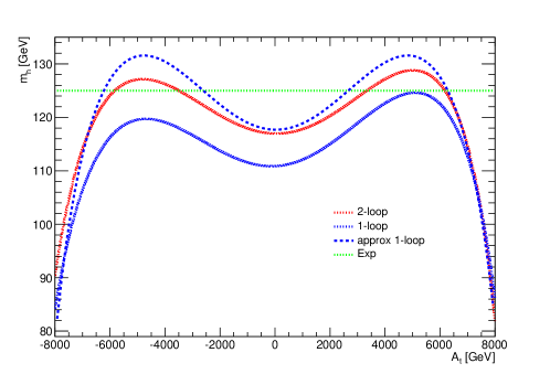
Figure 1: The prediction of $m_{h}$ at one– and two–loop precision as well as for the approximate one–loop is shown as function of $A_{t}$ together with the measured mass.

The procedure captures an essential feature of the inversion for $A_{t}$: in principle there are two $X^{2}_{t}$ solutions which, when real-valued and positive, lead to up to four different $A_{t}$ solutions. This well-known feature is illustrated in fig. 1 where we show the $m_{h}$ prediction for the full one–loop, two–loop and the approximate one–loop calculations. For the $m_{h}(A_{t})$ full one–loop and two–loop results, $A_{t}$ was varied and for each $A_{t}$ the EWSB minimisation was performed to derive the running mass of the CP–odd Higgs boson and the $\mu$ parameter. All other parameters were fixed to their cliff point values. For the approximate one–loop, the coefficients of eq. 10 were calculated for the cliff point, thus fixing $\overline{m}_{A}^{2}$ and $\mu$ and varying only $A_{t}$ in the square root of eq. 10 shown in the figure. For the measured Higgs boson there are four intersections with the prediction. The third intersection (from left to right) with the two-loop prediction is consistent with the $A_{t}$ cliff point value of 3.61 TeV.

Table 2: The result of the $A_{t}$ determination from $m_{h}$ using eq. 10 is shown. s3 corresponds to the nominal solution: the cliff point.

s1	$A_{t}$ [TeV]	-5.44
s2	$A_{t}$ [TeV]	-3.61
s3	$A_{t}$ [TeV]	2.87
s4	$A_{t}$ [TeV]	6.36

We turn now to the inverse approach of determining $A_{t}$ from eq. 10 when the measured $m_{h}$ is taken as input. The $A_{t}$ determination is illustrated in table 2. Four solutions are determined for $A_{t}$ as expected. The third solution s3 corresponds to the nominal solution: the cliff point. In each one of the solutions $\overline{m}_{A}^{2}$ and $\mu$ are those corresponding to the intersection of the two—loop Higgs mass with the measured $m_{h}$.

For the nominal $A_{t}$ in s3 eq. 10 leads to a Higgs mass larger than the two–loop Higgs mass prediction (see Fig.1). This is compensated by an $A_{t}$ value smaller than the nominal one: 2.87 TeV instead of 3.61 TeV. The use of the measured $m_{h}$ in the calculation therefore inevitably leads to a shift in $A_{t}$. Its calculated value is within 25% of the nominal value, a clear improvement compared to a blind guess. At the same time, it clearly illustrates that an accurate $A_{t}(m_{h})$ determination requires a more elaborate construction as compared to eq. 10, which we will describe next.

3.2 Full One–Loop: the HiggsMolar Function

For the full one–loop inversion the starting point is the (formally exact) eq. 7 which we rewrite here as an essentially quadratic equation in the CP-even Higgs squared masses,

$$m_{h,H}^{4}- m_{h,H}^{2}\left(({\cal M}^{2}_{s})_{{}_{11}}(p^{2})+({\cal M}^{2}_{s})_{{}_{22}}(p^{2})\right)$$ (14)

$$+({\cal M}^{2}_{s})_{{}_{11}}(p^{2})({\cal M}^{2}_{s})_{{}_{22}}(p^{2})-\left(({\cal M}^{2}_{s})_{{}_{12}}(p^{2})\right)^{2}|_{p^{2}=m^{2}_{h,H}}=0,$$

of which $m_{h}^{2}$ corresponds to the lighter mass solution. Here $({\cal M}^{2}_{s})_{{}_{ij}}(p^{2})$ denotes the real parts of the matrix element, and the solutions $p^{2}=m_{h,H}^{2}$ are real-valued. The $({\cal M}^{2}_{s})_{{}_{ij}}(p^{2})$’s extracted from eq. 3 include perturbatively complete loop corrections where the full one–loop Higgs boson self-energies, $\Pi_{ij}$, and tadpoles $t_{i}$ are taken from Pierce:1996zz . In the $\overline{\rm DR}$ scheme these expressions include contributions from all (s)particles (running) masses, resulting in a highly nonlinear dependence on $A_{t}$ from the stop sector. In particular the finite part of the one–loop scalar function $A_{0}$, occurring in the tadpoles and self-energies, has a rather involved $A_{t}$ dependence when its argument is the stop mass:

$$A_{0}(m_{\tilde{t}_{i}}) =m_{\tilde{t}_{i}}^{2}\left(1-\ln\left(\frac{m_{\tilde{t}_{i}}^{2}}{Q^{2}}\right)\right)$$ (15)

where $Q$ is the $\overline{\rm DR}$-scheme renormalization scale, and where from the stop sector diagonalization, the $\overline{\rm DR}$-scheme running stop masses can be written as

$$m_{\tilde{t}_{1,2}}^{2}=\frac{1}{2}\left(M^{2}\mp\sqrt{a_{s}A_{t}^{2}+b_{s}A_{t}+c_{s}}\right),$$ (16)

where

$$M^{2}=m_{\tilde{q}3_{L}}^{2}+m_{\tilde{t}_{R}}^{2}+2m_{t}^{2}+\frac{1}{2}m_{Z}^{2}\cos{2\beta},$$ (17)

$$a_{s}=4m_{t}^{2},$$

$$b_{s}=-8m_{t}^{2}\mu\cot\beta,$$

$$c_{s}=\left(m_{\tilde{q}3_{L}}^{2}-m_{\tilde{t}_{R}}^{2}+(\frac{1}{2}-\frac{4}{3}s_{W}^{2})m_{Z}^{2}\cos{2\beta}\right)^{2}+4m_{t}^{2}\mu^{2}\cot^{2}\beta,$$

are $A_{t}$ independent. The strategy is to rewrite eq. 14 as an equation for $A_{t}$ by extracting from eq. 3 the explicit polynomial $A_{t}$ dependencies or ”power counting” within each $\Pi_{ij}$ and $t_{i}$. On close inspection of the various contributions in e.g. Pierce:1996zz we identify:

1. terms depending linearly on $A_{t}$ (with coefficients identified by a superscript ’1’), originating from the $s_{k}$–$\tilde{t}_{i}$–$\tilde{t}_{j}$ couplings, $g_{s_{2}\tilde{t}_{1}\tilde{t}_{1}}$, $g_{s_{2}\tilde{t}_{2}\tilde{t}_{2}}$, $g_{s_{2}\tilde{t}_{1}\tilde{t}_{2}}$ which are given by

   $$g_{s_{2}\tilde{t}_{1}\tilde{t}_{1}} =c_{t}^{2}\,g_{s_{2}{\tilde{t}_{L}}{\tilde{t}_{L}}}+2c_{t}s_{t}\,g_{s_{2}{\tilde{t}_{L}}{\tilde{t}_{R}}}+s_{t}^{2}\,g_{s_{2}{\tilde{t}_{R}}{\tilde{t}_{R}}},$$ (18)

   $$g_{s_{2}\tilde{t}_{2}\tilde{t}_{2}} =s_{t}^{2}\,g_{s_{2}{\tilde{t}_{L}}{\tilde{t}_{L}}}-2c_{t}s_{t}\,g_{s_{2}{\tilde{t}_{L}}{\tilde{t}_{R}}}+c_{t}^{2}\,g_{s_{2}{\tilde{t}_{R}}{\tilde{t}_{R}}},$$

   $$g_{s_{2}\tilde{t}_{1}\tilde{t}_{2}} =s_{t}c_{t}\,(g_{s_{2}{\tilde{t}_{R}}{\tilde{t}_{R}}}-g_{s_{2}{\tilde{t}_{L}}{\tilde{t}_{L}}})+(c_{t}^{2}-s_{t}^{2})\,g_{s_{2}{\tilde{t}_{L}}{\tilde{t}_{R}}},$$

   $$g_{s_{2}{\tilde{t}_{L}}{\tilde{t}_{R}}} =\frac{y_{t}}{\sqrt{2}}A_{t},$$

   with $y_{t}$ the top quark Yukawa coupling, $s_{t}\equiv\sin\tilde{\theta}_{t}$, $c_{t}\equiv\cos\tilde{\theta}_{t}$, where $\tilde{\theta}_{t}$ denotes the stop mixing angle, $\tilde{t}_{1},\tilde{t}_{2}$ are the stop mass eigenstates, $\tilde{t}_{L}$, $\tilde{t}_{R}$ the gauge eigenstates, and $s_{k}$ are the neutral scalar states in the basis corresponding to eq. 3. Note that $g_{s_{2}{\tilde{t}_{R}}{\tilde{t}_{R}}}$, $g_{s_{2}{\tilde{t}_{L}}{\tilde{t}_{L}}}$ do not depend explicitly on $A_{t}$, their expressions can be found e.g. in Pierce:1996zz (denoted by $\lambda_{s_{2}{\tilde{u}_{L,R}}{\tilde{u}_{L,R}}},\lambda_{s_{2}{\tilde{u}_{L}}{\tilde{u}_{R}}}$ therein).

2. terms depending quadratically on $A_{t}$ (with coefficients identified by a superscript ’2’), originating from the $g_{s_{2}t_{i}t_{i}}^{2}$ that appear solely in $\Pi_{22}(p^{2})$;

3. terms depending on $\sqrt{a_{s}A_{t}^{2}+b_{s}A_{t}+c_{s}}$ (with coefficients identified by ’s’) originating from the $m_{\tilde{t}_{i}}^{2}$ in $A_{0}(m_{\tilde{t}_{i}})$;

4. a term containing $A_{t}\cdot\sqrt{a_{s}A_{t}^{2}+b_{s}A_{t}+c_{s}}$ (with coefficient identified by ’1s’) resulting from the occurrence of the product $g_{s_{2}t_{i}t_{i}}\times A_{0}(m_{\tilde{t}_{i}})$ appearing solely in $t_{2}$;

5. finally all remnant contributions with no (explicit) dependence or with logarithmic dependence on $A_{t}$, are identified by a ’0’ superscript. It is an important part of our strategy that in our $A_{t}$-power counting any “logarithmic” dependence $\sim\ln(M^{2}\mp\sqrt{a_{s}A_{t}^{2}+\cdots})$ on $A_{t}$ (such as in the second term of eq. 15, and in the one–loop scalar function $B_{0}$), as well as the other algebraic dependence on $A_{t}$ in $B_{0}$, are incorporated exactly as they stand within the coefficients of the above listed relevant $A_{t}$ powers. In the following we dub these dependencies “residual”. The dependence of the stop mixing angle $\tilde{\theta}_{t}$ on $A_{t}$ is also treated as residual, since it enters in eq. 18 through $c_{t}$ and $s_{t}$ that remain obviously bounded functions of $A_{t}$.

According to the previous $A_{t}$ power counting, within the relevant (one–loop) $\Pi_{ij}$ and $t_{i}$ individual contributions, there are no higher degree monomials in $A_{t}$ than the $A_{t}^{k}$ identified above with $k\leq 2$. This gives the following formal decomposition of the tadpoles and self-energies:

$$\frac{t_{1}}{v_{1}}=t_{1}^{(s)}\sqrt{a_{s}A_{t}^{2}+b_{s}A_{t}+c_{s}}+t_{1}^{(0)}$$

$$\frac{t_{2}}{v_{2}}=t_{2}^{(1s)}A_{t}\sqrt{a_{s}A_{t}^{2}+b_{s}A_{t}+c_{s}}+t_{2}^{(1)}A_{t}+t_{2}^{(s)}\sqrt{a_{s}A_{t}^{2}+b_{s}A_{t}+c_{s}}+t_{2}^{(0)}$$

$$\Pi_{11}=\pi_{11}^{(s)}\sqrt{a_{s}A_{t}^{2}+b_{s}A_{t}+c_{s}}+\pi_{11}^{(0)}$$ (19)

$$\Pi_{12}=\pi_{12}^{(1)}A_{t}+\pi_{12}^{(0)}$$

$$\Pi_{22}=\pi_{22}^{(2)}A_{t}^{2}+\pi_{22}^{(1)}A_{t}+\pi_{22}^{(s)}\sqrt{a_{s}A_{t}^{2}+b_{s}A_{t}+c_{s}}+\pi_{22}^{(0)}$$

Equation 19 is simply a convenient rewriting of already available exact one–loop expressions, no contributions are ignored. Using eq. 19 to display the algebraic dependence on $A_{t}$ in eq. 14, the following molar-shaped function $\mathrm{HiggsMolar}(A_{t})$, which should consistently vanish for any $A_{t}$ solution, is obtained:

$$\mathrm{HiggsMolar}(A_{t})= C_{3}A_{t}^{3}+C_{2}A_{t}^{2}+C_{1}A_{t}+C_{0}$$

$$+(R_{2}A_{t}^{2}+R_{1}A_{t}+R_{0})\sqrt{a_{s}A_{t}^{2}+b_{s}A_{t}+c_{s}}=0.$$ (20)

The $\mathrm{HiggsMolar}$ is shown as function of $A_{t}$ in fig. 2. For each $A_{t}$ the coefficients are recalculated. The four other curves show the behavior of the function if the coefficients determined at the intersections of the $\mathrm{HiggsMolar}$ with the line $\mathrm{HiggsMolar}=0$ are used in the vicinity of the intersections. The curves illustrate the variation of the coefficients.

This equation can in principle be used separately either for the lighter or for the heavier CP-even Higgs masses, as clear from eq. 14. Hereafter we are only considering the lighter Higgs mass at $\sim 125\mathrm{GeV}$ as input. The $C_{i}$ and $R_{i}$ coefficients are easily identified upon use of eqs. 19, 3 and 14. They contain all the residual $A_{t}$ dependencies quoted above, neglecting all imaginary parts as justified in footnote 1.

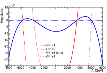
Figure 2: The distribution of the $\mathrm{HiggsMolar}$ is shown as function of $A_{t}$: calculating the coefficients of eq. 20 for each $A_{t}$ (solid blue curve); fixing the coefficients of eq. 20 at the four $A_{t}$ solutions (red curves). For the four solutions, given by the intersections with the dotted blue line, only the $A_{t}$ range around the solution is shown by the red curves.

The cubic term results from the product $(t_{1}-\Pi_{11})\times t_{2}$ present in $({\cal M}^{2}_{s})_{11}({\cal M}^{2}_{s})_{22}$, with a coefficient $C_{3}$ given by

$$C_{3}=4\overline{m}_{t}^{2}(t_{1}^{(s)}-\pi_{11}^{(s)})t_{2}^{(1s)}.$$ (21)

In particular, in contrast with eq. 10 and unless performing in eq. 20 an expansion in $X_{t}$, explicit $X_{t}^{4}\sim A_{t}^{4}$ terms cannot occur within the exact eq. 14 as the equation does not involve squares of terms of the type ’2’ or ’1s’.

The general form of the other $C_{i}$ and $R_{i}$ coefficients is given in appendix A. These coefficients have a more involved dependence on (differences of) the quantities $\pi_{ij}^{(0,s,1,2)}$ and $t_{i}^{(0,s,1,1s)}$ entering eq. 19. The relevant one–loop expressions of the latter are also given in appendix A. They allow to track the residual dependence on $A_{t}$ and the absence of some finite combinations in relation to the expected cancellation of the quadratic divergences in softly-broken SUSY. The full one–loop explicit dependence on $A_{t}$ is thus included in eq. 20. A further implicit dependence on $A_{t}$ will originate from the two EWSB conditions Eqs. (8), (9) when imposed beyond the tree-level, due to the presence of $\overline{m}_{A}^{2}$ as well as $\mu$ in the $C_{i}$ and $R_{i}$ coefficients. In particular, the $t_{2}$-tadpole dependence in $\overline{m}_{A}^{2}$ will induce, through the term $\overline{m}_{11}^{2}\times t_{2}$ appearing in the cross-product $({\cal M}^{2}_{s})_{11}({\cal M}^{2}_{s})_{22}$ in eq. 14, an effectively quartic dependence on $A_{t}$ for large $A_{t}$, not explicit in eq. 20. This entails solving simultaneously eq. 20 and the EWSB constraints Eqs. (8) and (9), which we will perform numerically in a consistent way as described in section 4.1. Other implicit dependencies on $A_{t}$ are discussed in section 3.5. Hereafter we ignore momentarily these issues and focus solely on the resolution of eq. 20.

3.3 Full One-Loop Inversion: the Fixed Point Algorithm

To solve eq. 20 for $A_{t}$, a fixed point iterative method is used. For this purpose we define

$$\mathrm{C_{FP}}(A_{t})=-\frac{1}{C_{3}}\Big{(} C_{2}A_{t}^{2}+C_{1}A_{t}+C_{0}$$ (22)

$$+(R_{2}A_{t}^{2}+R_{1}A_{t}+R_{0})\sqrt{a_{s}A_{t}^{2}+b_{s}A_{t}+c_{s}}\Big{)},$$

and rewrite eq. 20 as

$$A_{t}=\sqrt[3]{\mathrm{C_{FP}}(A_{t})}.$$ (23)

It is then clear that finding all the real-valued solutions of eq. 20 is equivalent to determining all the fixed points $A_{t}=A_{t}^{FP}$, satisfying $\mathrm{L_{FP}}(A_{t}^{FP})=A_{t}^{FP}$, of the function $\mathrm{L_{FP}}$ defined by

$$\mathrm{L_{FP}}(A_{t})\equiv\sqrt[3]{\mathrm{C_{FP}}(A_{t})},$$ (24)

with only real-valued cubic roots allowed.

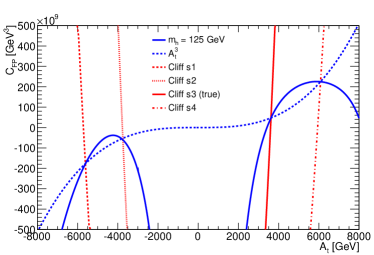
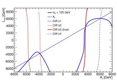
Figure 3: The distributions of the functions $\mathrm{C_{FP}}$ and $\mathrm{L_{FP}}$ are shown as function of $A_{t}$: calculating the coefficients of eq. 20 for each $A_{t}$ (solid blue curve); fixing the coefficients of eq. 20 at the four $A_{t}$ solutions (red curves). For the four solutions, given by the intersections with the dotted blue line, only the $A_{t}$ range around the solution is shown by the red curves.

To determine the fixed points one starts from a guess value $A_{t,0}=A_{t}^{Guess}$ and studies the convergence of the sequence $A_{t,i+1}=\mathrm{L_{FP}}(A_{t_{i}})$. The iterations return unambiguously real-valued $A_{t}$ as a consequence of the definition of $\mathrm{L_{FP}}$, eq. 24. As we will specify in more detail in section 4, appropriate $A_{t}$-guess values, not too far from the exact solutions, are those obtained from our approximate one-loop eq. 10 that already captures the multi-solution structure. However, even if starting relatively close to the exact solutions, the method will catch only the attractive fixed points and can thus miss some, otherwise acceptable, $A_{t}$ solutions.

One expects typically four distinct solutions as illustrated in Figure 3 for the stop cliff benchmark: The functions $\mathrm{C_{FP}}(A_{t})$ and $\mathrm{L_{FP}}(A_{t})$, in blue, intersect the dotted blue lines at the fixed points of these functions, corresponding to the four $A_{t}$ solutions that are consistent with $m_{h}=125\mathrm{GeV}$. For the blue curve the coefficients $C_{i}$ and $R_{i}$ of the two fixed point functions were recalculated at each $A_{t}$. For the four red curves these coefficients are frozen at their values calculated at the intersection of the blue curve with the blue dotted line, for $A_{t}$ varying in the vicinity of the intersection.

The dotted blue line on Figure 3-right being the bisector, it follows that the slope of $\mathrm{L_{FP}}$ at its fixed points is alternatively greater or smaller than one. We label the solutions $s1,s2,s3,s4$ ordered in ascending in $A_{t}$. Given that $\mathrm{L_{FP}}$ takes negative values for very large $\lvert A_{t}\rvert$, the slopes of $\mathrm{L_{FP}}$ at $s1$ and $s3$ are necessarily greater than one and those at $s2$ and $s4$ less than one. $s1$ and $s3$ are thus repulsive fixed points. In contrast, $s2$ and $s4$ will be either attractive if the slope is between $-1$ and $1$, or alternating/repulsive if the slope is less than $-1$. The slope at $s2$ is typically less than zero due to the strong variation of $\mathrm{L_{FP}}$ in the vicinity of $\lvert A_{t}\rvert\sim 0$. It follows that the iterative procedure on $\mathrm{L_{FP}}$ as described above will always miss solutions $s1$ and $s3$ while capturing at best two solutions, namely $s2$ and $s4$, provided furthermore the initial guess values $A_{t}^{Guess}$ close enough to $s2$ and $s4$ to feel their attracting character. If a guess point is chosen anywhere above $s3$ the iterations will repel it from $s3$ and converge to $s4$. If chosen below $s1$ it will be repelled to the left and the procedure will never converge. Finally, if chosen between $s1$ and $s3$ then, depending on the behaviour around $s2$, the convergence to $s4$ (and occasionally to $s2$ if its slope is greater than $-1$) may or may not occur.

In order to ensure convergence and be able to capture all solutions, we consider a generalized family $\mathrm{L_{FP}}_{\tau}$ of functions parametrized by $\tau\neq 0$ as follows:

$$\mathrm{L_{FP}}_{\tau}(A_{t})=\frac{1}{\tau}(\mathrm{L_{FP}}(A_{t})-A_{t})+A_{t}.$$ (25)

Any fixed point of $\mathrm{L_{FP}}$ is also a fixed point of $\mathrm{L_{FP}}_{\tau}$ and vice versa, for any value of $\tau$.

Moreover from

$$\mathrm{L_{FP}}^{\prime}_{\tau}(A_{t})=1+\frac{\mathrm{L_{FP}}^{\prime}(A_{t})-1}{\tau},$$ (26)

follows that one can always choose $\tau$ in such a way that $\mathrm{L_{FP}}^{\prime}_{\tau}(A_{t}^{FP})$ lies in the interval $[-1,1]$ for any given value of $\mathrm{L_{FP}}^{\prime}(A_{t}^{FP})$. Thus the advantage of $\mathrm{L_{FP}}_{\tau}$ is that all fixed points of $\mathrm{L_{FP}}$ can be made attractive with respect to $\mathrm{L_{FP}}_{\tau}$ for appropriately chosen values of $\tau$. In this case an iteration over the sequence $A_{t,i+1}=\mathrm{L_{FP}}_{\tau}(A_{t_{i}})$ is guaranteed to converge on $A_{t}^{FP}$, at least when the initial guess values are not too far from the solution. However, $A_{t}^{FP}$ is not known in advance, even less $\mathrm{L_{FP}}^{\prime}(A_{t}^{FP})$. Without this knowledge, a rough strategy to converge on a given solution could be to choose:

• $\tau\gtrsim 1$ for $s4$

• $\tau\ll-1$ for $s1,s3$

• $\tau\gg 1$ for $s2$.

Actually one can do better by determining optimal values of $\tau$ from the knowledge of the local variation of $\mathrm{L_{FP}}$ during the iterative procedure. A numerical estimate $\Delta\mathrm{L_{FP}}/\Delta A_{t}$ of the first derivative of $\mathrm{L_{FP}}$ with respect to $A_{t}$ can in principle be calculated at any given step during the iterations on $A_{t}$ at moderate computational cost. Then choosing the $\tau$ parameter as follows

$$\frac{\Delta\mathrm{L_{FP}}}{\Delta A_{t}}-1<0:\tau=+\left\lvert\frac{\Delta\mathrm{L_{FP}}}{\Delta A_{t}}-1\right\rvert,$$

$$\frac{\Delta\mathrm{L_{FP}}}{\Delta A_{t}}-1>0:\tau=-\left\lvert\frac{\Delta\mathrm{L_{FP}}}{\Delta A_{t}}-1\right\rvert,$$ (27)

ensures that an estimate of the derivative of $\mathrm{L_{FP}}_{\tau}$ is close to zero, cf. eq. 26. Since this estimate is in practice not at the fixed point, eq. 27 is not sufficient to guarantee convergence. However, it approximates a necessary condition, fulfilling a convergence criterion discussed in appendix B, see eq. 45. This allows to make any fixed point attractive, provided initial guess values are not too far from that fixed point. A simple and efficient algorithm will be implemented along these lines, as described in Section 4.

3.4 Dominant Two–Loop Inversion

The extension of the above exact one–loop method to the two–loop contributions is rather straightforward. The latter corrections depend dominantly on the strong, weak and third generation Yukawa couplings $y_{i}$, leading to terms of $\mathcal{O}$($\alpha_{s,i}$)$\times\mathcal{O}$(One–loop), where $\alpha_{i}\equiv y_{i}^{2}/(4\pi)$. In the standard fixed-order (diagrammatic) $m_{h}$ calculations, $\Pi_{ij}^{(2-loop)}$ and $t_{i}^{(2-loop)}$ contributions are added to the ${\cal M}^{2}_{s}$ matrix elements which enter the squared Higgs boson mass equation shown in eq. 14.

Due to the extra loop suppression factor, at any scale relevant for the MSSM spectrum calculation where either $\alpha_{s}(Q)$ or $\alpha_{i}(Q)$ remain moderate, the two–loop contributions are a moderate correction relative to the one–loop contributions (even if including those is obviously very relevant for a more precise comparison between the MSSM prediction and the measured $m_{h}$ value. For instance typically for the benchmark cliff point, restricting to exact one–loop would give $m_{h}\sim 118$ GeV instead of $\sim 125$ GeV as in Table 1.) Thus, for the $A_{t}(m_{h})$ inversion, rather than trying to extract specific quite involved $A_{t}$ dependencies from the $\Pi_{ij}^{(2-loop)}$ and $t_{i}^{(2-loop)}$ contributions, the latter are incorporated just as they contribute to Eq.(3): more precisely, within the above algorithm the available two–loop contributions are formally treated as if they were independent of $A_{t}$, therefore concretely incorporated as additional contributions to either $t_{i}^{(0)}$ or $\pi_{ij}^{(0)}$ in eq. 19:

$$t_{i}^{(0)}\to t_{i}^{(0)}+t_{i}^{(2-loop)},\;\;\pi_{ij}^{(0)}\to\pi_{ij}^{(0)}+\Pi_{ij}^{(2-loop)}.$$ (28)

This is then corrected iteratively for the true $A_{t}$ dependence. The seven coefficients entering the $\mathrm{HiggsMolar}$($A_{t}$) function of eq. 20 can now be computed incorporating consistently two–loop contributions.

3.5 Including Higher Orders and Refinements

At this stage the inversion is formally ’exact’ at the considered (perturbative) level of theoretical precision taken for the $t_{i}$ tadpoles and self-energy contributions $\Pi_{ij}$, namely full one–loop and only the dominant two–loop contributions. It is a straightforward matter to incorporate either more complete two–loop and/or higher (3–loop) contributions, by considering those contributions similarly $A_{t}$ independent, since their actual $A_{t}$ dependence, independent of its complexity, is screened by tiny perturbative expansion coefficients. As long as higher order corrections are obtained diagrammatically in the form of self-energy or tadpole contributions, these could be included explicitly by adding them to the $t^{(0)}_{i}$ and $\pi^{(0)}_{ij}$ contributions.

It is well known that sizeable theoretical uncertainties in $m_{h}$ determinations (customarily taken as $\sim\pm 2-3$ GeV in phenomenological analyses) are due to presently unknown higher order contributions, discrepancies between different renormalization schemes, etc (see e.g. Degrassi:2002fi ; Allanach:2004rh , or for more recent analyses Allanach:2018fif ; Bahl:2019hmm , as well as the recent updated discussion in Slavich:2020zjv ). Given these uncertainties, one might question the importance of devising a very accurate inversion procedure. The answer is obvious: not to introduce artificially further uncertainties in the determination of $A_{t}(m_{h})$ than there are from a given content of higher order contributions included in the standard $m_{h}$ determination. Related to this, there remains one subtlety to consider: Even at one–loop level, there are extra implicit $A_{t}$ dependencies that would not be accounted for by the previous algorithm, if one relied solely on the procedure leading to eq. 20. Indeed, the self-energies and tadpoles also depend typically on SM-like gauge and Yukawa couplings, as well as other running $\overline{\rm DR}$ parameters ($s_{W}$, $m_{W}$), which are affected by threshold corrections, depending themselves on the MSSM parameters, therefore depending on $A_{t}$ in a highly nontrivial way in this case. While all these threshold corrections give contributions that are formally of higher (at least two–loop) order within the loop self-energy and tadpole expressions, they can induce a numerical inconsistency bias if not incorporated in the inversion, slightly shifting the resulting $A_{t}(m_{h})$ with respect to its actual ’reference’ value in a standard top-down calculation. This, as well as the other residual or implicit dependencies on $A_{t}$ already mentioned in section 3.2, are, however, consistently taken into account in the full algorithm as we explain next.

4 The Full Inversion Algorithm

The algorithm has been implemented in SuSpect3 Djouadi:2002ze ; Brooijmans:2012yi . SuSpect3 is a public spectrum calculator for multiple supersymmetric models that includes, within eq. 3 for $m_{h}$, the $\overline{\rm DR}$ radiative corrections at full one–loop and dominant two-loop orders (involving for the latter the QCD and third family Yukawa contributions, but at vanishing $p^{2}$). Other MSSM spectrum calculators are, non-exhaustively, SOFTSUSY Allanach:2001kg , SPHENO  Porod:2003um ; Porod:2011nf ; Staub:2017jnp , FeynHiggs Heinemeyer:1998yj ; Heinemeyer:1998np ; Heinemeyer:2000nz ; Bahl:2018qog , and FlexibleSUSY Athron:2014yba . Note that on top of fixed-order calculations including some contributions beyond the above mentioned two-loop order, some of these codes (FeynHiggs, SPHENO, FlexibleSUSY) also include resummations of large logarithms in an EFT approach for the Higgs mass calculations, thus with an a priori increased precision for large soft-supersymmetry breaking mass scenarios.

Before describing the full inversion algorithm, let us first briefly recall the procedure to determine the spectrum in the MSSM. This involves solving the RGE to evolve the parameters between the EWSB scale ($Q_{\mathrm{EWSB}}$) and the scale given by the mass of the Z boson ($m_{Z}$), as well as solving the EWSB equations eq. 8, eq. 9 at $Q_{\mathrm{EWSB}}$. Radiative corrections to the supersymmetric particle and Higgs boson masses are calculated at $Q_{\mathrm{EWSB}}$. Supersymmetric radiative corrections to Standard Model parameters, the most important in the present study being the top yukawa coupling, are calculated at $m_{Z}$.

For EWSB three variants have been implemented. If $\overline{m}^{2}_{H_{d}}$, $\overline{m}^{2}_{H_{u}}$ and the sign of $\mu$ are given as input, the running mass squared $\overline{m}_{A}^{2}$ and the Higgs mass parameter $\mu$ are calculated. Alternatively $\mu$ and either the pole mass $m_{A}$ or the tree-level running mass squared $\overline{m}_{A}^{2}$ can be given to calculate $\overline{m}^{2}_{H_{d}}$, $\overline{m}^{2}_{H_{u}}$.

Both the RGE evolution and the EWSB calculations are implemented as iterations. The convergence is tested on the stability of $\overline{m}_{A}^{2}$ or $\overline{m}_{H_{u}}^{2}$ between successive iterations. The choice depends on the input parameter set chosen.

We recall that for a precise calculation of the MSSM spectrum in the standard top-down approach, it is essential that some of the relevant running parameters at a given scale, and consequently the physical (pole) masses, are calculated iteratively, as these parameters are nontrivially modified by radiative corrections, which in turn depend on potentially all MSSM parameters. There is also an iteration between the EWSB and $m_{Z}$ scales, since important radiative corrections, depending themselves on the MSSM spectrum, are incorporated to extract the $\overline{\rm DR}$-scheme gauge and Yukawa couplings upon matching their experimentally measured values. The convergence criterion for the RGE iteration depends on the choice for the EWSB parameters.

4.1 Algorithm

In the $m_{h}$MSSM the $A_{t}(m_{h})$ determination algorithm extends the previously described calculation of the relevant EWSB parameters of the MSSM in SuSpect3. The determination of $A_{t}$ has been added to this already necessarily iterative structure as the determination of an additional parameter. The algorithm to determine $A_{t}$ is independent of the parameter input choice. In the following the numerical examples are given for an input of $\overline{m}^{2}_{H_{d}}$, $\overline{m}^{2}_{H_{u}}$ and the sign of $\mu$. The calculation starts with the RGE evolution from the Z boson scale to a high scale. $A_{t}$ is initialized arbitrarily to a fixed value (10 GeV) as the parameter will be determined after the RGE evolution to $Q_{\mathrm{EWSB}}$. The procedure is similar to the initialization of $\mu$.

First the MSSM EWSB calculations are performed, i.e., $\mu$ and $\overline{m}_{A}^{2}$ are determined, and then $A_{t}$ is determined. This procedure is repeated until convergence is reached according to the MSSM criteria, i.e., $\mu$ is stable and therefore $\overline{m}_{A}^{2}$ is stable as well.

At the first and second RGE iteration the approximate one–loop eq. 10 with the measured $m_{h}$ as input is solved to extract a new $A_{t}$ as explained in section 3.1. Taking into account the newly determined $A_{t}$, the RGE evolution to the Z mass scale is performed. Radiative corrections are calculated, in particular to the top yukawa terms. The parameters are then RGE evolved to the high scale. The second RGE iteration therefore starts at the high scale with the $A_{t}$ value derived from the approximate one-loop algorithm in the first iteration.

For the cliff point, table 2 shows that the correct $A_{t}$ is within 25% of the calculated value. The use of eq. 10 is preferred over the fixed point algorithm as the radiative corrections used depend on $y_{t}\cdot\mu$. This allows to stabilize quickly $y_{t}$ with an approximate $A_{t}$ at low computational cost. Using the full radiative calculations at this stage would lead to longer iterations as the variations of both $\mu$ and $A_{t}$ take longer to stabilize.

For the third and all following RGE iterations the full radiative calculations are used for EWSB, combined with the fixed point algorithm described in sections 3.3 and 3.4 to determine $A_{t}$. For each new $A_{t}$, obtained from $\mathrm{L_{FP}}_{\tau}$, eq. 25, the tree-level stop sector and the Higgs sector including radiative corrections are recalculated. This has the advantage that not only the leading terms of $\mathrm{L_{FP}}$, eq. 24, are taken into account, but also both the residual and implicit $A_{t}$ dependencies in the coefficients $C_{i}$ and $R_{i}$, as explained previously. The recalculation of the stop sector and the Higgs sector for each iteration brings the function from the red curves closer to the blue (nominal) curves in figs. 2 and 3.

The convergence depends on the $\tau$ parameter. When the full radiative corrections are used in the algorithm, an estimate $\Delta\mathrm{L_{FP}}/\Delta A_{t}$ of the first derivative of $\mathrm{L_{FP}}$ with respect to $A_{t}$ is calculated numerically at the end of the iteration on $A_{t}$. The iterations are stopped when the relative change of $A_{t}$ between the last and the current value is smaller than a threshold. Numerical values are given below. The $\tau$ parameter is then adjusted according to eq. 27 which is used in the next determination of $A_{t}$.

4.2 Proof of Concept

Table 3: The result of the Higgs inversion algorithm is shown for the stop cliff. The true point is s3. As a cross check the $m_{h}$ values shown are the result of the standard $m_{h}(A_{t})$ calculation with the $A_{t}$ obtained from the input $m_{h}$ parameter.

stop cliff	s1	s2	s3	s4
$A_{t}$ [GeV]	-5617.3	-3796.1	3609.7	6082.5
$m_{h}$ [GeV]	125.012	125.012	125.012	125.012

As proof of concept the calculation is performed for all four possible solutions using the full algorithm. The $A_{t}$ is first determined via the approximate one-loop calculation for the first two RGE iterations and then the fixed point algorithm is used for all following iterations. $A_{t}$ is refined at each step. To converge on the spectrum calculation the RGE iterations are stopped once $\overline{m}_{A}$ is stabilized to the permil level. The EWSB iterations are stopped when $\mu$ has converged at permil level. The iterations on $A_{t}$ are run with a convergence criterion of permil.

The results of the full algorithm are shown in table 3. Four solutions are obtained as expected. The calculation of $A_{t}$ and the calculated $m_{h}$ are in excellent agreement with the expected values.

In point s3 the deviation of the calculated $A_{t}$ value from the expected value in table 1 is far smaller than convergence criterion on $A_{t}$ suggests. This is the consequence of the hierarchical structure of the iterations. The iteration on $A_{t}$ is at the lowest level, therefore the calculation of $A_{t}$ is also refined for each EWSB and (times) RGE iteration until the running mass of the A boson and the $\mu$ parameter have converged. This leads to a higher precision than naively expected.

4.3 Scan Settings

If the algorithm is used in a multidimensional scan of supersymmetric parameters, an example using SuSpect3 is in Butter:2015fqa , the $m_{h}$MSSM ensures that no spectrum calculation will be performed for parameter sets incompatible with the measured central value of $m_{h}$. This leads to a reduction of the parameter space allowed for $A_{t}$. However such a calculation, due to the iteration on $A_{t}$, has a calculational overhead compared to an MSSM spectrum calculation.

Given that the experimental uncertainty on the $m_{h}$ measurement is of the order of 0.1 GeV and additionally the theoretical uncertainty is about 2 GeV, the following calculations have been performed with reduced precision: the RGE iterations are stopped when percent level convergence on $\overline{m}_{A}$ has been reached. All other convergence definitions remain unchanged. These are the standard settings used in Suspect.

To illustrate the calculational overhead the MSSM calculation is compared to the $m_{h}$MSSM calculation for s3. The number of RGE iterations is increased from four to six. The algorithm typically adds one additional iteration to each EWSB calculation on top of the three for the standard algorithm, i.e., a total of 27 iterations is necessary compared to 13 for the standard settings. The calculation of $A_{t}$ at the first two RGE iterations as a direct calculation of the approximate solution is not computationally intensive. When the fixed point method is used, for the first two RGE iterations, at the first EWSB iteration six and four calculations are necessary to converge on the fixed point to the required accuracy. For the subsequent EWSB iterations typically only one or two iterations on $A_{t}$ are necessary. For the last two RGE iterations for all EWSB iterations only one or two $A_{t}$ calculations are necessary. For half of EWSB iterations, a single calculation of $A_{t}$ is sufficient. The reduction of the number of iterations on $A_{t}$ as the RGE and EWSB iterations progress illustrates the convergence of the algorithm.

Table 4: The result of the Higgs inversion algorithm for the three definitions of EWSB input variables is shown. s3 is the true point. The calculated $A_{t}$ and the resulting $m_{h}$ are listed for all calculations.

EWSB		s1	s2	s3	s4
$m^{2}_{H_{d}}$, $m^{2}_{H_{u}}$, sign($\mu$)	$A_{t}$ [GeV]	-5617.8	-3795.0	3610.5	6085.9
	$m_{h}$ [GeV]	125.012	125.012	125.012	125.012
$m_{A}^{2}(Q)$, $\mu$	$A_{t}$ [GeV]	-5606.9	-3795.1	3610.7	6090.1
	$m_{h}$ [GeV]	125.012	125.012	125.012	125.012
$m_{A}$, $\mu$	$A_{t}$ [GeV]	-5607.2	-3794.7	3610.7	6089.9
	$m_{h}$ [GeV]	125.012	125.012	125.012	125.012

In table 4 the results on $A_{t}$ and the calculated $m_{h}$ are shown for the reduced precision setting of the algorithm. The maximal difference between the calculated Higgs masses is less than 1 MeV, i.e., largely sufficient given the experimental error.

The two EWSB calculations with the $\mu$ parameter as input lead to almost identical results for all $A_{t}$ solutions. The two EWSB calculations with $\mu$ use $\overline{m}_{H_{u}}^{2}$ as variable to test convergence whereas the other EWSB calculation uses $\overline{m}_{A}^{2}$ to stop the RGE iterations. The calculation is performed with a fixed convergence precision. The impact on the $m_{h}$ value for a change of $\overline{m}^{2}_{H_{u}}$ and $\overline{m}_{A}^{2}$ is not identical. Therefore the results for EWSB with the A boson mass, tree level or pole, can be different with respect to the calculation with the Higgs mass parameters. For the true solution s3, the maximal deviation for all EWSB variants is only two tenth of a permil , at 0.7 GeV with respect to the true $A_{t}$ of the cliff point table 1.

4.4 Beyond the Cliff

The cliff point is a favorable situation as four distinct solutions exist. A parameter set can lead to a situation where the local minimum of the Higgs boson mass in the vicinity of $A_{t}=0$ GeV is larger than the $m_{h}$ parameter input. Alternatively the $m_{h}$ parameter could be higher than either one or both of the maxima of fig. 1.

To test the validity of the algorithm beyond the proof of concept in the cliff point, the input $m_{h}$ parameter was varied. The algorithm was slightly extended for $m_{h}$ values close to the maxima and the local minimum by a bisection algorithm. To ensure a logical coherence of the results, the regions of validity for $A_{t}$ are defined for the four solutions:

• s1: $-\infty$ to $A_{t}(m_{h}^{max}(A_{t}<0))$

• s2: $A_{t}(m_{h}^{max}(A_{t}<0))$ to $A_{t}(m_{h}^{min}(A_{t}\sim 0))$

• s3: $A_{t}(m_{h}^{min}(A_{t}\sim 0))$ to $A_{t}(m_{h}^{max}(A_{t}>0))$

• s4: $A_{t}(m_{h}^{max}(A_{t}>0))$ to $\infty$

If the $m_{h}$ parameter is out of reach, the closest $A_{t}$ in the region is used.

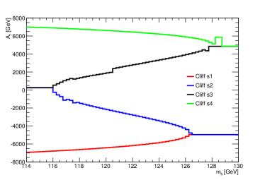
Figure 4: The result of the determination of $A_{t}$ is shown as function of the chosen $m_{h}$. The determination is performed separately for the four solutions. The histograms are stacked from s1 (bottom) to s4 (top), the horizontal lines at constant $A_{t}$ at the transition between the regions show only the top color.

The result of a scan of $m_{h}$ values between 112 GeV and 128 GeV is shown in fig. 4. The four solutions are correctly reconstructed over the full range. For s2 and s3 the lowest parameter values cannot be reached, therefore the $A_{t}$ value of the local minimal mass is determined. A similar feature is observed when the parameter is greater than the maximal $m_{h}$ at 2-loop precision shown in fig. 1. In this case $A_{t}$ corresponding to the maximal mass achievable for the parameters is determined, resulting in a line parallel to the x–axis. The steps correspond to cases where the $\mu$ parameter and the CP-odd scalar Higgs boson mass have converged to a slightly different value which leads to a step in $A_{t}$ and an offset in the predicted $m_{h}$, smaller than the systematic of 2 GeV typically used in scans of the parameter space. In total 256 inversions are shown of which only 3 have not converged correctly. These points are all located in regions where a larger $m_{h}$ than possible was requested (horizontal lines at $A_{t}\approx-4.95$ TeV and $A_{t}\approx 4.85$ TeV) and for two the algorithm returned an error for non convergence. Since the step size of the scan of 0.25 GeV is smaller than the error on the Higgs mass of about 2 GeV, posterior distributions of $A_{t}$ also give an additional handle on the outliers.

fig. 4 shows $A_{t}$ as multi-valued function of $m_{h}$ covering the same parameter space as fig. 1. This shows that the inversion, based on the exact calculation, works, validating the use of the approximate one–loop calculation as a first guess. However, there could be problematic parameter sets for which the guess points are not sufficiently close to the fixed points to ensure convergence. An alternative algorithm relying on the knowledge of $A_{t}(m_{h}^{max}(A_{t}<0)),A_{t}(m_{h}^{min}(A_{t}\sim 0))$ and $A_{t}(m_{h}^{max}(A_{t}>0))$, combined with global rather than local criteria, could then be used.

4.5 Beyond the Fixed-Order Approximation

Our inversion strategy is built upon fixed-order diagrammatic results, in particular upon the knowledge of the analytical form of the exact one–loop contribution to the Higgs mass. In more recent developments of MSSM Higgs mass radiative corrections, there are, however, configurations where an EFT approach is better suited for a reliable estimate of the Higgs mass, like typically when considering an MSSM setup with (very) heavy scalars (see e.g. Slavich:2020zjv for a recent review). In this case, if for instance a heavy stop sector is integrated out from the low-energy EFT, a direct analytical relation between $m_{h}$ and $A_{t}$ will be essentially lost. Nevertheless, an inversion procedure can still be carried out: The needed relation will reside now in the matching condition at the boundary scale between the light and heavy sectors for the quartic Higgs coupling, from which the multi-$A_{t}$ solutions can be retrieved analytically.

4.6 Beyond the CP-conserving Case

If complex phases are allowed for the MSSM parameters, the dependence of $m_{h}$ on $A_{t}$ will be in general significantly modified due to loop induced CP-violating mixings among all the neutral Higgs states. The ensuing $3\times 3$ mass matrix after identifying the Goldstone boson, implies an analytical expression of $m_{h}^{2}$ given by a root of a cubic equation, quite different from that obtained from the diagonalization of eq. 3. Our approach can be easily extended to this case in the (experimentally likely) configuration where the MSSM spectrum, and in particular the charged Higgs mass, are much heavier than the $125\mathrm{GeV}$ state. As well known, in this case the CP-violating mixing is essentially confined to the two heavy neutral states sector, see e.g. Pilaftsis_1999 , and the phenomenology (mass, couplings) of the lightest would-be CP-even state becomes essentially the same as in the CP-conserving MSSM. In this limit, taking $A_{t}$ and $\mu$ complex (which is sufficient to account for the physically relevant phases, denoted $\phi_{A_{t}}$ and $\phi_{\mu}$), the functional dependence of $m_{h}$ on $\lvert A_{t}\rvert$ will be the same as that on $A_{t}$ in the CP-conserving case. The only difference is the reduction of some coefficients by cosine factors, (typically occurrences of $(\mu A_{t})^{n}$ become $(\left\lvert\mu\right\lvert\left\lvert A_{t}\right\lvert)^{n}\cos n(\phi_{\mu}+\phi_{A_{t}})$, otherwise even powers $A_{t}^{2n}$ become $\left\lvert A_{t}\right\lvert^{2n}$, etc.). Modulo these modifications in eqs. 10 and 20, our algorithm will work exactly as before, to determine $\left\lvert A_{t}\right\lvert$ (and/or $-\left\lvert A_{t}\right\lvert$) solutions from $m_{h}$, given $\phi_{A_{t}}$ (and or $\phi_{A_{t}}\pm\pi$), a complex $\mu$, and the other parameters of the MSSM. Beyond this (relative decoupling) limit, the algorithm can still provide an educated guess for $\pm\lvert A_{t}\rvert$ input, within a more general numerical algorithm for the CP-violating MSSM.

5 Conclusion

The discovery and precise measurement of the Higgs boson motivates the redefinition of the MSSM as $m_{h}$MSSM. The algorithm presented in this paper replaces the trilinear coupling of the stop sector $A_{t}$ with the measured $m_{h}$ as input parameter.

The simplified expression of the radiative corrections to $m_{h}$ and the exact full one–loop with the leading two–loop corrections are assembled in an algorithm to calculate $A_{t}$. The algorithm has been applied to a benchmark point showing that the four solutions are determined with the expected precision. A single parameter scan with $m_{h}$ as scan parameter shows that the $A_{t}$ dependence is correctly reconstructed.

The general structure of the algorithm could also be applied to other parameters. Using the $m_{h}$MSSM may speed up the exploration of supersymmetric parameter space by ensuring the compatibility of all calculated spectra with the experimentally measured $m_{h}$. Future work will center on applying the algorithm in multi-parameter scans.

Acknowledgments We would like to thank Steve Muanza for his collaboration and input at an early stage of this study, as well as the PESBLADE working group of the OCEVU Labex for useful discussions. We also acknowledge instructive exchanges with Pietro Slavich. This work benefited from partial support of the OCEVU Labex (ANR-11-LABX-0060) and the A*MIDEX project (ANR-11-IDEX-0001-02) funded by the “Investissements d’Avenir” French government program managed by the ANR.

Appendix A The coefficients of $\mathrm{HiggsMolar}$$(A_{t})$

We give hereafter the explicit dependence of the coefficients appearing in eq. 20 on the various $\pi_{ij}^{(..)}$, tadpoles and running mass parameters, as well as the relevant combinations of the latter in terms of the MSSM parameters of the stop sector.

$$C_{0}[A_{t}]= c_{s}(\pi_{11}^{(s)}-t_{1}^{(s)})(\pi_{22}^{(s)}-t_{2}^{(s)})+(m_{h}^{2}+\pi_{11}^{(0)}-t_{1}^{(0)}-\overline{m}_{11}^{2})$$ (29)

$$\cdot(m_{h}^{2}+\pi_{22}^{(0)}-t_{2}^{(0)}-\overline{m}_{22}^{2})-(\pi_{12}^{(0)}-\overline{m}_{12}^{2})^{2},$$

$$C_{1}[A_{t}]= (\pi_{11}^{(s)}-t_{1}^{(s)})(b_{s}(\pi_{22}^{(s)}-t_{2}^{(s)})-c_{s}t_{2}^{(1s)})+(\pi_{22}^{(1)}-t_{2}^{(1)})$$

$$\cdot(m_{h}^{2}+\pi_{11}^{(0)}-t_{1}^{(0)}-\overline{m}_{11}^{2})+2\pi_{12}^{(1)}(\overline{m}_{12}^{2}-\pi_{12}^{(0)}),$$

$$C_{2}[A_{t}]= (\pi_{11}^{(s)}-t_{1}^{(s)})(a_{s}(\pi_{22}^{(s)}-t_{2}^{(s)})-b_{s}t_{2}^{(1s)})$$

$$+\pi_{22}^{(2)}(m_{h}^{2}+\pi_{11}^{(0)}-t_{1}^{(0)}-\overline{m}_{11}^{2})-(\pi_{12}^{(1)})^{2},$$

$$C_{3}[A_{t}]= a_{s}(t_{1}^{(s)}-\pi_{11}^{(s)})t_{2}^{(1s)},$$

$$R_{0}[A_{t}]= (\pi_{11}^{(s)}-t_{1}^{(s)})(m_{h}^{2}+\pi_{22}^{(0)}-t_{2}^{(0)}-\overline{m}_{22}^{2})$$

$$+(\pi_{22}^{(s)}-t_{2}^{(s)})(m_{h}^{2}+\pi_{11}^{(0)}-t_{1}^{(0)}-\overline{m}_{11}^{2}),$$

$$R_{1}[A_{t}]= (t_{1}^{(s)}-\pi_{11}^{(s)})(t_{2}^{(1)}-\pi_{22}^{(1)})+(t_{1}^{(0)}-\pi_{11}^{(0)}+\overline{m}_{11}^{2}-m_{h}^{2})t_{2}^{(1s)},$$

$$R_{2}[A_{t}]= \pi_{22}^{(2)}(\pi_{11}^{(s)}-t_{1}^{(s)}),$$

where the $\overline{m}_{ij}^{2}$ are given by eqs. 4, 5 and 6.

Relying on the full one–loop results (and partly on the notations) of Pierce:1996zz , we extract the relevant contributions of the self-energies and tadpoles:

$$16\pi^{2}(t_{1}^{(0)}-\pi_{11}^{(0)})= \frac{3}{\sqrt{2}}\frac{g_{2}c_{t}s_{t}y_{t}\mu M^{2}}{c_{\beta}M_{W}}\ln\left(\frac{m_{\tilde{t}_{1}}}{m_{\tilde{t}_{2}}}\right)$$

$$-3\sum_{i,j=1}^{2}g_{s_{1}\tilde{t}_{i}\tilde{t}_{j}}^{2}B_{0}\left(m_{\tilde{t}_{i}},m_{\tilde{t}_{j}}\right)+\cdots,$$ (30)

$$16\pi^{2}(t_{1}^{(s)}-\pi_{11}^{(s)}) =\frac{3}{\sqrt{2}}\frac{g_{2}c_{t}s_{t}y_{t}\mu}{c_{\beta}M_{W}}\left(1-\ln\left(\frac{m_{\tilde{t}_{1}}m_{\tilde{t}_{2}}}{Q^{2}}\right)\right),$$ (31)

$$16\pi^{2}(t_{2}^{(0)}-\pi_{22}^{(0)})=-3\Big{(} \sum_{i=1}^{2}(\Delta g_{i})^{2}B_{0}\left(m_{\tilde{t}_{i}},m_{\tilde{t}_{i}}\right)$$

$$+2(\Delta g_{12})^{2}B_{0}\left(m_{\tilde{t}_{1}},m_{\tilde{t}_{2}}\right)\Big{)}+\cdots,$$ (32)

$$16\pi^{2}(t_{2}^{(s)}-\pi_{22}^{(s)}) =0,$$ (33)

$$16\pi^{2}(t_{2}^{(1)}-\pi_{22}^{(1)})= \frac{3}{\sqrt{2}}\frac{g_{2}y_{t}c_{t}s_{t}M^{2}}{s_{\beta}M_{W}}\ln\left(\frac{m_{\tilde{t}_{2}}}{m_{\tilde{t}_{1}}}\right)$$

$$-6\sqrt{2}y_{t}\Big{(}c_{t}s_{t}\left(\Delta g_{1}B_{0}\left(m_{\tilde{t}_{1}},m_{\tilde{t}_{1}}\right)-\Delta g_{2}B_{0}\left(m_{\tilde{t}_{2}},m_{\tilde{t}_{2}}\right)\right)$$

$$~{}~{}~{}~{}~{}~{}~{}~{}~{}~{}~{}~{}~{}+(c_{t}^{2}-s_{t}^{2})\Delta g_{12}B_{0}\left(m_{\tilde{t}_{1}},m_{\tilde{t}_{2}}\right)\Big{)},$$ (34)

$$16\pi^{2}t_{2}^{(1s)} =\frac{3}{\sqrt{2}}\frac{g_{2}y_{t}c_{t}s_{t}}{s_{\beta}M_{W}}\left(\ln\left(\frac{m_{\tilde{t}_{1}}m_{\tilde{t}_{2}}}{Q^{2}}\right)-1\right),$$ (35)

$$16\pi^{2}\pi_{22}^{(2)}=3y_{t}^{2}\Big{(} 2c_{t}^{2}s_{t}^{2}\left(B_{0}\left(m_{\tilde{t}_{1}},m_{\tilde{t}_{1}}\right)+B_{0}\left(m_{\tilde{t}_{2}},m_{\tilde{t}_{2}}\right)\right)$$

$$+(c_{t}^{2}-s_{t}^{2})^{2}B_{0}\left(m_{\tilde{t}_{1}},m_{\tilde{t}_{2}}\right)\Big{)},$$ (36)

$$16\pi^{2}\pi_{12}^{(0)}=3\Big{(} g_{s_{1}\tilde{t}_{1}\tilde{t}_{1}}\Delta g_{1}B_{0}\left(m_{\tilde{t}_{1}},m_{\tilde{t}_{1}}\right)+g_{s_{1}\tilde{t}_{2}\tilde{t}_{2}}\Delta g_{2}B_{0}\left(m_{\tilde{t}_{2}},m_{\tilde{t}_{2}}\right)$$

$$+g_{s_{1}\tilde{t}_{1}\tilde{t}_{2}}\Delta g_{12}B_{0}\left(m_{\tilde{t}_{1}},m_{\tilde{t}_{2}}\right)\Big{)}+\cdots,~{}~{}~{}~{}~{}~{}~{}~{}~{}~{}~{}~{}~{}~{}~{}~{}~{}~{}~{}~{}~{}$$ (37)

$$16\pi^{2}\pi_{12}^{(1)}=\frac{3}{\sqrt{2}}y_{t}\Big{(} 2c_{t}s_{t}\left(g_{s_{1}\tilde{t}_{1}\tilde{t}_{1}}B_{0}\left(m_{\tilde{t}_{1}},m_{\tilde{t}_{1}}\right)-g_{s_{1}\tilde{t}_{2}\tilde{t}_{2}}B_{0}\left(m_{\tilde{t}_{2}},m_{\tilde{t}_{2}}\right)\right)$$

$$+2(c_{t}^{2}-s_{t}^{2})g_{s_{1}\tilde{t}_{1}\tilde{t}_{2}}B_{0}\left(m_{\tilde{t}_{1}},m_{\tilde{t}_{2}}\right)\Big{)}$$ (38)

where we have defined

$$\Delta g_{1} \equiv c_{t}^{2}g_{s_{2}\tilde{t}_{L}\tilde{t}_{L}}+s_{t}^{2}g_{s_{2}\tilde{t}_{R}\tilde{t}_{R}},$$ (39)

$$\Delta g_{2} \equiv s_{t}^{2}g_{s_{2}\tilde{t}_{L}\tilde{t}_{L}}+c_{t}^{2}g_{s_{2}\tilde{t}_{R}\tilde{t}_{R}},$$

$$\Delta g_{12} \equiv c_{t}s_{t}(g_{s_{2}\tilde{t}_{R}\tilde{t}_{R}}-g_{s_{2}\tilde{t}_{L}\tilde{t}_{L}}).$$

$s_{\beta}$ and $c_{\beta}$ stand for $\sin\beta$ and $\cos\beta$, and all other quantities have been defined previously, see also eqs. 16, LABEL:eq:asetc and 18. The ellipses indicate contributions from the Higgs/Higgsino, gauge/gaugino and other scalar/fermion sectors, that do not have a direct dependence on $A_{t}$. The couplings $g_{s_{1}\tilde{t}_{i}\tilde{t}_{j}}$ are related to $g_{s_{1}{\tilde{t}_{L,R}}{\tilde{t}_{L,R}}},g_{s_{1}{\tilde{t}_{L}}{\tilde{t}_{R}}}$ as in eq. 18, but do not depend explicitly on $A_{t}$. All parameters appearing in the above expressions are understood to be running in the $\overline{\rm DR}$ scheme, and $Q$ is the corresponding renormalization scale. The dependence on $p^{2}$, cf. eq. 3, taken here at $p^{2}=m_{h}^{2}$, is in the $B_{0}$ functions with the shorthand notation $B_{0}(m_{1},m_{2})\equiv B_{0}(m_{h},m_{1},m_{2})$, see also footnote 1.

Note finally that the vanishing of $t_{2}^{(s)}-\pi_{22}^{(s)}$, cf. eq. 33, together with the fact that $M^{2}$ appears exclusively with $\ln\left(\frac{m_{\tilde{t}_{1}}}{m_{\tilde{t}_{2}}}\right)$, eqs. 30 and 34, and $\sqrt{a_{s}A_{t}^{2}+b_{s}A_{t}+c_{s}}$ exclusively with $\ln\left(\frac{m_{\tilde{t}_{1}}m_{\tilde{t}_{2}}}{Q^{2}}\right)$, eqs. 31 and 35, are a direct consequence of the cancellation of the quadratic divergences before renormalization as expected in softly-broken SUSY. Indeed, in this case the stop sector contributions from the $A_{0}$ function can occur only in the combination $A_{0}(m_{\tilde{t}_{1}})-A_{0}(m_{\tilde{t}_{2}})$.

Appendix B Convergence Criterion

A fixed point $x_{\rm FP}$ of a function $F$, satisfying $F(x_{\rm FP})=x_{\rm FP}$, can be determined iteratively as the limit of a sequence defined by ${x}_{i+1}=F(x_{i})$ and an initial guess $x_{0}$, only if the fixed point is attractive, i.e. $-1\leq F^{\prime}(x_{\rm FP})\leq 1$. We sketch here how to proceed in the more general cases of non-attractive fixed points:

Define

$$F_{\tau}(x)=\frac{(\tau-1)x+F(x)}{\tau},\rm{\;with}\,\tau\neq 0,$$ (40)

and

$$F(x)-F(x_{0})=(x-x_{0})K(x,x_{0})$$ (41)

with

$$K(x_{0},x_{0})=F^{\prime}(x)_{\lvert x=x_{0}}.$$ (42)

Let us consider two distinct sequences given by

$${x}_{i+1}=F_{\tau}(x_{i})\text{~{}and~{}}{y}_{i+1}=F_{\tau}(y_{i}),\ (\text{with}\ x_{0}\neq y_{0}),$$ (43)

and study the variation $F_{\tau}(x_{n})-F_{\tau}(y_{n})$ after $n$ iterations. One finds straightforwardly upon repeated use of eqs. 40, 41 and 43:

$$F_{\tau}(x_{n})-F_{\tau}(y_{n}) = (x_{n}-y_{n})\left(1+\frac{K(x_{n},y_{n})-1}{\tau}\right),$$

$$= \left(F_{\tau}(x_{n-1})-F_{\tau}(y_{n-1})\right)\left(1+\frac{K(x_{n},y_{n})-1}{\tau}\right),$$

$$\vdots$$

$$F_{\tau}(x_{n})-F_{\tau}(y_{n}) = (x_{0}-y_{0})\prod_{i=0}^{n}\left(1+\frac{K(x_{i},y_{i})-1}{\tau}\right).$$ (44)

It follows from Eq. (44) that

choosing $$\tau \left|1+\frac{K(x_{i},y_{i})-1}{\tau}\right\rvert 1 i 0 n$$ such that is sufficiently smaller than for a sufficiently large set of ’s between and , (45)

leads to

$$\left\lvert\prod_{i=0}^{n}\left(1+\frac{K(x_{i},y_{i})-1}{\tau}\right)\right\rvert\ll 1,$$ (46)

and the two sequences $x_{i}$ and $y_{i}$ converge towards each other aftern $n$ iterations within a prescribed numerical precision. In particular, choosing $y_{0}=x_{\rm FP}$ yields a constant sequence $\{y_{i}\}=\{x_{\rm FP}\}$, and $x_{i}$ converges to the fixed point $x_{\rm FP}$. This completes the proof that by using the auxiliary function $F_{\tau}$, one can in principle always optimize the choice of $\tau$ depending on the variations of $F$ , so as to converge to $x_{\rm FP}$ for a given initial guess value $x_{0}$, even when dealing with non-attractive fixed points of $F$. It should be stressed that $K(x_{i},y_{i})$ is not always a very good estimate of the local variation of $F$ since the two sequences $\{x_{i}\}$ and $\{y_{i}\}$ do not necessarily start off close to each other. Nonetheless, it will become so after a few iterations if $\tau$ satisfies the criterion (45). In particular, for the constant sequence $\{y_{i}\}\equiv\{x_{\rm FP}\}$, the successive values of $K$ correspond to variations with respect to the same reference point $x_{\rm FP}$ which is of course not yet known. However, if the initial guess point $x_{0}$ is sufficiently close to $x_{\rm FP}$, one can in practice use $K(x_{i},x_{i+1})$ instead of $K(x_{i},x_{\rm FP})$ to optimize $\tau$ piece-wise. With this in mind, we can apply the above procedure to the case of $\mathrm{L_{FP}}$, where the quantity $\left(1+\frac{K(x_{i},x_{i+1})-1}{\tau}\right)$, with $K(x_{i},x_{i+1}))=\Delta\mathrm{L_{FP}}/\Delta x$ being an estimate of $\mathrm{L_{FP}}^{\prime}(x_{\rm FP})$ for $x_{i}$ sufficiently close to $x_{\rm FP}$, is clearly a discretized version of $\mathrm{L_{FP}}^{\prime}_{\tau}(x_{i})$ as given by eq. 26. A simple numerical algorithm can thus be devised, based on eq. 27 as described at the end of Section 3.3.

References

- \bibcommenthead
- (1) Aad, G., et al.: Observation of a new particle in the search for the Standard Model Higgs boson with the ATLAS detector at the LHC. Phys. Lett. B 716, 1–29 (2012) https://arxiv.org/abs/1207.7214 [hep-ex]. https://doi.org/10.1016/j.physletb.2012.08.020
- (2) Chatrchyan, S., et al.: Observation of a New Boson at a Mass of 125 GeV with the CMS Experiment at the LHC. Phys. Lett. B 716, 30–61 (2012) https://arxiv.org/abs/1207.7235 [hep-ex]. https://doi.org/10.1016/j.physletb.2012.08.021
- (3) Aaboud, M., et al.: Measurement of the Higgs boson mass in the and channels with TeV collisions using the ATLAS detector. Phys. Lett. B 784, 345–366 (2018) https://arxiv.org/abs/1806.00242 [hep-ex]. https://doi.org/10.1016/j.physletb.2018.07.050
- (4) Sirunyan, A.M., et al.: Measurements of properties of the Higgs boson decaying into the four-lepton final state in pp collisions at TeV. JHEP 11, 047 (2017) https://arxiv.org/abs/1706.09936 [hep-ex]. https://doi.org/10.1007/JHEP11(2017)047
- (5) Aad, G., et al.: Combined Measurement of the Higgs Boson Mass in Collisions at and 8 TeV with the ATLAS and CMS Experiments. Phys. Rev. Lett. 114, 191803 (2015) https://arxiv.org/abs/1503.07589 [hep-ex]. https://doi.org/10.1103/PhysRevLett.114.191803
- (6) Zyla, P.A., et al.: Review of Particle Physics. PTEP 2020(8), 083C01 (2020). https://doi.org/10.1093/ptep/ptaa104
- (7) Schael, S., et al.: Precision electroweak measurements on the resonance. Phys. Rept. 427, 257–454 (2006) https://arxiv.org/abs/hep-ex/0509008. https://doi.org/10.1016/j.physrep.2005.12.006
- (8) Dubovyk, I., Freitas, A., Gluza, J., Riemann, T., Usovitsch, J.: Electroweak pseudo-observables and Z-boson form factors at two-loop accuracy. JHEP 08, 113 (2019) https://arxiv.org/abs/1906.08815 [hep-ph]. https://doi.org/10.1007/JHEP08(2019)113
- (9) Kneur, J.-L., Moultaka, G.: Inverting the supersymmetric standard model spectrum: From physical to Lagrangian gaugino parameters. Phys. Rev. D 59, 015005 (1999) https://arxiv.org/abs/hep-ph/9807336. https://doi.org/10.1103/PhysRevD.59.015005
- (10) Kneur, J.-L., Moultaka, G.: Phases in the gaugino sector: Direct reconstruction of the basic parameters and impact on the neutralino pair production. Phys. Rev. D 61, 095003 (2000) https://arxiv.org/abs/hep-ph/9907360. https://doi.org/10.1103/PhysRevD.61.095003
- (11) Kneur, J.-L., Sahoury, N.: Bottom-Up Reconstruction Scenarios for (un)constrained MSSM Parameters at the LHC. Phys. Rev. D 79, 075010 (2009) https://arxiv.org/abs/0808.0144 [hep-ph]. https://doi.org/10.1103/PhysRevD.79.075010
- (12) Djouadi, A., Maiani, L., Moreau, G., Polosa, A., Quevillon, J., Riquer, V.: The post-Higgs MSSM scenario: Habemus MSSM? Eur. Phys. J. C 73, 2650 (2013) https://arxiv.org/abs/1307.5205 [hep-ph]. https://doi.org/10.1140/epjc/s10052-013-2650-0
- (13) Djouadi, A.: The Anatomy of electro-weak symmetry breaking. II. The Higgs bosons in the minimal supersymmetric model. Phys. Rept. 459, 1–241 (2008) https://arxiv.org/abs/hep-ph/0503173. https://doi.org/10.1016/j.physrep.2007.10.005
- (14) Heinemeyer, S.: MSSM Higgs physics at higher orders. Int. J. Mod. Phys. A 21, 2659–2772 (2006) https://arxiv.org/abs/hep-ph/0407244. https://doi.org/10.1142/S0217751X06031028
- (15) Slavich, P., et al.: Higgs-mass predictions in the MSSM and beyond. Eur. Phys. J. C 81(5), 450 (2021) https://arxiv.org/abs/2012.15629 [hep-ph]. https://doi.org/10.1140/epjc/s10052-021-09198-2
- (16) Chankowski, P.H., Pokorski, S., Rosiek, J.: Charged and neutral supersymmetric Higgs boson masses: Complete one loop analysis. Phys. Lett. B 274, 191–198 (1992). https://doi.org/%****␣HiggsInversion.bbl␣Line␣300␣****10.1016/0370-2693(92)90522-6
- (17) Chankowski, P.H., Pokorski, S., Rosiek, J.: Complete on-shell renormalization scheme for the minimal supersymmetric Higgs sector. Nucl. Phys. B 423, 437–496 (1994) https://arxiv.org/abs/hep-ph/9303309. https://doi.org/10.1016/0550-3213(94)90141-4
- (18) Dabelstein, A.: The One loop renormalization of the MSSM Higgs sector and its application to the neutral scalar Higgs masses. Z. Phys. C 67, 495–512 (1995) https://arxiv.org/abs/hep-ph/9409375. https://doi.org/10.1007/BF01624592
- (19) Pierce, D.M., Bagger, J.A., Matchev, K.T., Zhang, R.: Precision corrections in the minimal supersymmetric standard model. Nucl. Phys. B 491, 3–67 (1997) https://arxiv.org/abs/hep-ph/9606211. https://doi.org/10.1016/S0550-3213(96)00683-9
- (20) Hempfling, R., Hoang, A.H.: Two loop radiative corrections to the upper limit of the lightest Higgs boson mass in the minimal supersymmetric model. Phys. Lett. B 331, 99–106 (1994) https://arxiv.org/abs/hep-ph/9401219. https://doi.org/10.1016/0370-2693(94)90948-2
- (21) Heinemeyer, S., Hollik, W., Weiglein, G.: QCD corrections to the masses of the neutral CP - even Higgs bosons in the MSSM. Phys. Rev. D 58, 091701 (1998) https://arxiv.org/abs/hep-ph/9803277. https://doi.org/10.1103/PhysRevD.58.091701
- (22) Heinemeyer, S., Hollik, W., Weiglein, G.: The Masses of the neutral CP - even Higgs bosons in the MSSM: Accurate analysis at the two loop level. Eur. Phys. J. C 9, 343–366 (1999) https://arxiv.org/abs/hep-ph/9812472. https://doi.org/10.1007/s100529900006
- (23) Heinemeyer, S., Hollik, W., Weiglein, G.: Precise prediction for the mass of the lightest Higgs boson in the MSSM. Phys. Lett. B 440, 296–304 (1998) https://arxiv.org/abs/hep-ph/9807423. https://doi.org/10.1016/S0370-2693(98)01116-2
- (24) Heinemeyer, S., Hollik, W., Rzehak, H., Weiglein, G.: High-precision predictions for the MSSM Higgs sector at O(alpha(b) alpha(s)). Eur. Phys. J. C 39, 465–481 (2005) https://arxiv.org/abs/hep-ph/0411114. https://doi.org/10.1140/epjc/s2005-02112-6
- (25) Zhang, R.-J.: Two loop effective potential calculation of the lightest CP even Higgs boson mass in the MSSM. Phys. Lett. B 447, 89–97 (1999) https://arxiv.org/abs/hep-ph/9808299. https://doi.org/10.1016/S0370-2693(98)01575-5
- (26) Espinosa, J.R., Zhang, R.-J.: MSSM lightest CP even Higgs boson mass to O(alpha(s) alpha(t)): The Effective potential approach. JHEP 03, 026 (2000) https://arxiv.org/abs/hep-ph/9912236. https://doi.org/10.1088/1126-6708/2000/03/026
- (27) Espinosa, J.R., Zhang, R.-J.: Complete two loop dominant corrections to the mass of the lightest CP even Higgs boson in the minimal supersymmetric standard model. Nucl. Phys. B 586, 3–38 (2000) https://arxiv.org/abs/hep-ph/0003246. https://doi.org/10.1016/S0550-3213(00)00421-1
- (28) Degrassi, G., Slavich, P., Zwirner, F.: On the neutral Higgs boson masses in the MSSM for arbitrary stop mixing. Nucl. Phys. B 611, 403–422 (2001) https://arxiv.org/abs/hep-ph/0105096. https://doi.org/10.1016/S0550-3213(01)00343-1
- (29) Brignole, A., Degrassi, G., Slavich, P., Zwirner, F.: On the O(alpha(t)**2) two loop corrections to the neutral Higgs boson masses in the MSSM. Nucl. Phys. B 631, 195–218 (2002) https://arxiv.org/abs/hep-ph/0112177. https://doi.org/10.1016/S0550-3213(02)00184-0
- (30) Brignole, A., Degrassi, G., Slavich, P., Zwirner, F.: On the two loop sbottom corrections to the neutral Higgs boson masses in the MSSM. Nucl. Phys. B 643, 79–92 (2002) https://arxiv.org/abs/hep-ph/0206101. https://doi.org/10.1016/S0550-3213(02)00748-4
- (31) Dedes, A., Slavich, P.: Two loop corrections to radiative electroweak symmetry breaking in the MSSM. Nucl. Phys. B 657, 333–354 (2003) https://arxiv.org/abs/hep-ph/0212132. https://doi.org/%****␣HiggsInversion.bbl␣Line␣550␣****10.1016/S0550-3213(03)00173-1
- (32) Dedes, A., Degrassi, G., Slavich, P.: On the two loop Yukawa corrections to the MSSM Higgs boson masses at large tan beta. Nucl. Phys. B 672, 144–162 (2003) https://arxiv.org/abs/hep-ph/0305127. https://doi.org/10.1016/j.nuclphysb.2003.08.033
- (33) Degrassi, G., Heinemeyer, S., Hollik, W., Slavich, P., Weiglein, G.: Towards high precision predictions for the MSSM Higgs sector. Eur. Phys. J. C 28, 133–143 (2003) https://arxiv.org/abs/hep-ph/0212020. https://doi.org/10.1140/epjc/s2003-01152-2
- (34) Martin, S.P.: Complete Two Loop Effective Potential Approximation to the Lightest Higgs Scalar Boson Mass in Supersymmetry. Phys. Rev. D 67, 095012 (2003) https://arxiv.org/abs/hep-ph/0211366. https://doi.org/%****␣HiggsInversion.bbl␣Line␣600␣****10.1103/PhysRevD.67.095012
- (35) Martin, S.P.: Strong and Yukawa two-loop contributions to Higgs scalar boson self-energies and pole masses in supersymmetry. Phys. Rev. D 71, 016012 (2005) https://arxiv.org/abs/hep-ph/0405022. https://doi.org/10.1103/PhysRevD.71.016012
- (36) Borowka, S., Hahn, T., Heinemeyer, S., Heinrich, G., Hollik, W.: Momentum-dependent two-loop QCD corrections to the neutral Higgs-boson masses in the MSSM. Eur. Phys. J. C 74(8), 2994 (2014) https://arxiv.org/abs/1404.7074 [hep-ph]. https://doi.org/10.1140/epjc/s10052-014-2994-0
- (37) Degrassi, G., Di Vita, S., Slavich, P.: Two-loop QCD corrections to the MSSM Higgs masses beyond the effective-potential approximation. Eur. Phys. J. C 75(2), 61 (2015) https://arxiv.org/abs/1410.3432 [hep-ph]. https://doi.org/10.1140/epjc/s10052-015-3280-5
- (38) Martin, S.P.: Three-loop corrections to the lightest Higgs scalar boson mass in supersymmetry. Phys. Rev. D 75, 055005 (2007) https://arxiv.org/abs/hep-ph/0701051. https://doi.org/10.1103/PhysRevD.75.055005
- (39) Harlander, R.V., Kant, P., Mihaila, L., Steinhauser, M.: Higgs boson mass in supersymmetry to three loops. Phys. Rev. Lett. 100, 191602 (2008) https://arxiv.org/abs/0803.0672 [hep-ph]. https://doi.org/10.1103/PhysRevLett.101.039901
- (40) Kant, P., Harlander, R.V., Mihaila, L., Steinhauser, M.: Light MSSM Higgs boson mass to three-loop accuracy. JHEP 08, 104 (2010) https://arxiv.org/abs/1005.5709 [hep-ph]. https://doi.org/10.1007/JHEP08(2010)104
- (41) Harlander, R.V., Klappert, J., Voigt, A.: Higgs mass prediction in the MSSM at three-loop level in a pure context. Eur. Phys. J. C 77(12), 814 (2017) https://arxiv.org/abs/1708.05720 [hep-ph]. https://doi.org/10.1140/epjc/s10052-017-5368-6
- (42) Aguilar-Saavedra, J.A., et al.: Supersymmetry parameter analysis: SPA convention and project. Eur. Phys. J. C 46, 43–60 (2006) https://arxiv.org/abs/hep-ph/0511344. https://doi.org/10.1140/epjc/s2005-02460-1
- (43) Aad, G., et al.: Search for squarks and gluinos in final states with jets and missing transverse momentum using 139 fb-1 of =13 TeV collision data with the ATLAS detector. JHEP 02, 143 (2021) https://arxiv.org/abs/2010.14293 [hep-ex]. https://doi.org/10.1007/JHEP02(2021)143
- (44) Aad, G., et al.: Search for electroweak production of charginos and sleptons decaying into final states with two leptons and missing transverse momentum in TeV collisions using the ATLAS detector. Eur. Phys. J. C 80(2), 123 (2020) https://arxiv.org/abs/1908.08215 [hep-ex]. https://doi.org/10.1140/epjc/s10052-019-7594-6
- (45) Sirunyan, A.M., et al.: Search for supersymmetry in proton-proton collisions at 13 TeV in final states with jets and missing transverse momentum. JHEP 10, 244 (2019) https://arxiv.org/abs/1908.04722 [hep-ex]. https://doi.org/10.1007/JHEP10(2019)244
- (46) Tumasyan, A., et al.: Search for electroweak production of charginos and neutralinos in proton-proton collisions at = 13 TeV. JHEP 04, 147 (2022) https://arxiv.org/abs/2106.14246 [hep-ex]. https://doi.org/10.1007/JHEP04(2022)147
- (47) Sirunyan, A.M., et al.: Search for supersymmetry in final states with two oppositely charged same-flavor leptons and missing transverse momentum in proton-proton collisions at 13 TeV. JHEP 04, 123 (2021) https://arxiv.org/abs/2012.08600 [hep-ex]. https://doi.org/10.1007/JHEP04(2021)123
- (48) Aad, G., et al.: Search for a scalar partner of the top quark in the all-hadronic plus missing transverse momentum final state at TeV with the ATLAS detector. Eur. Phys. J. C 80(8), 737 (2020) https://arxiv.org/abs/2004.14060 [hep-ex]. https://doi.org/10.1140/epjc/s10052-020-8102-8
- (49) Sirunyan, A.M., et al.: Search for top squark production in fully-hadronic final states in proton-proton collisions at 13 TeV. Phys. Rev. D 104(5), 052001 (2021) https://arxiv.org/abs/2103.01290 [hep-ex]. https://doi.org/10.1103/PhysRevD.104.052001
- (50) Ellis, J.R., Ridolfi, G., Zwirner, F.: Radiative corrections to the masses of supersymmetric Higgs bosons. Phys. Lett. B 257, 83–91 (1991). https://doi.org/10.1016/0370-2693(91)90863-L
- (51) Haber, H.E., Hempfling, R.: Can the mass of the lightest Higgs boson of the minimal supersymmetric model be larger than m(Z)? Phys. Rev. Lett. 66, 1815–1818 (1991). https://doi.org/10.1103/PhysRevLett.66.1815
- (52) Okada, Y., Yamaguchi, M., Yanagida, T.: Renormalization group analysis on the Higgs mass in the softly broken supersymmetric standard model. Phys. Lett. B 262, 54–58 (1991). https://doi.org/10.1016/0370-2693(91)90642-4
- (53) Carena, M., Espinosa, J.R., Quiros, M., Wagner, C.E.M.: Analytical expressions for radiatively corrected Higgs masses and couplings in the MSSM. Phys. Lett. B 355, 209–221 (1995) https://arxiv.org/abs/hep-ph/9504316. https://doi.org/10.1016/0370-2693(95)00694-G
- (54) Carena, M., Quiros, M., Wagner, C.E.M.: Effective potential methods and the Higgs mass spectrum in the MSSM. Nucl. Phys. B 461, 407–436 (1996) https://arxiv.org/abs/hep-ph/9508343. https://doi.org/10.1016/0550-3213(95)00665-6
- (55) Haber, H.E., Hempfling, R., Hoang, A.H.: Approximating the radiatively corrected Higgs mass in the minimal supersymmetric model. Z. Phys. C 75, 539–554 (1997) https://arxiv.org/abs/hep-ph/9609331. https://doi.org/%****␣HiggsInversion.bbl␣Line␣950␣****10.1007/s002880050498
- (56) Carena, M., Haber, H.E., Heinemeyer, S., Hollik, W., Wagner, C.E.M., Weiglein, G.: Reconciling the two loop diagrammatic and effective field theory computations of the mass of the lightest CP - even Higgs boson in the MSSM. Nucl. Phys. B 580, 29–57 (2000) https://arxiv.org/abs/hep-ph/0001002. https://doi.org/10.1016/S0550-3213(00)00212-1
- (57) Heinemeyer, S., Hollik, W., Weiglein, G.: FeynHiggsFast: A Program for a fast calculation of masses and mixing angles in the Higgs sector of the MSSM (2000) https://arxiv.org/abs/hep-ph/0002213
- (58) Skands, P.Z., et al.: SUSY Les Houches accord: Interfacing SUSY spectrum calculators, decay packages, and event generators. JHEP 07, 036 (2004) https://arxiv.org/abs/hep-ph/0311123. https://doi.org/10.1088/1126-6708/2004/07/036
- (59) Allanach, B.C., Djouadi, A., Kneur, J.L., Porod, W., Slavich, P.: Precise determination of the neutral Higgs boson masses in the MSSM. JHEP 09, 044 (2004) https://arxiv.org/abs/hep-ph/0406166. https://doi.org/10.1088/1126-6708/2004/09/044
- (60) Allanach, B.C., Voigt, A.: Uncertainties in the Lightest Even Higgs Boson Mass Prediction in the Minimal Supersymmetric Standard Model: Fixed Order Versus Effective Field Theory Prediction. Eur. Phys. J. C 78(7), 573 (2018) https://arxiv.org/abs/1804.09410 [hep-ph]. https://doi.org/10.1140/epjc/s10052-018-6046-z
- (61) Bahl, H., Heinemeyer, S., Hollik, W., Weiglein, G.: Theoretical uncertainties in the MSSM Higgs boson mass calculation. Eur. Phys. J. C 80(6), 497 (2020) https://arxiv.org/abs/1912.04199 [hep-ph]. https://doi.org/10.1140/epjc/s10052-020-8079-3
- (62) Djouadi, A., Kneur, J.-L., Moultaka, G.: SuSpect: A Fortran code for the supersymmetric and Higgs particle spectrum in the MSSM. Comput. Phys. Commun. 176, 426–455 (2007) https://arxiv.org/abs/hep-ph/0211331. https://doi.org/10.1016/j.cpc.2006.11.009
- (63) Brooijmans, G., et al.: Les Houches 2011: Physics at TeV Colliders New Physics Working Group Report, 221–463 (2012) https://arxiv.org/abs/1203.1488 [hep-ph]
- (64) Allanach, B.C.: SOFTSUSY: a program for calculating supersymmetric spectra. Comput. Phys. Commun. 143, 305–331 (2002) https://arxiv.org/abs/hep-ph/0104145. https://doi.org/10.1016/S0010-4655(01)00460-X
- (65) Porod, W.: SPheno, a program for calculating supersymmetric spectra, SUSY particle decays and SUSY particle production at e+ e- colliders. Comput. Phys. Commun. 153, 275–315 (2003) https://arxiv.org/abs/hep-ph/0301101. https://doi.org/10.1016/S0010-4655(03)00222-4
- (66) Porod, W., Staub, F.: SPheno 3.1: Extensions including flavour, CP-phases and models beyond the MSSM. Comput. Phys. Commun. 183, 2458–2469 (2012) https://arxiv.org/abs/1104.1573 [hep-ph]. https://doi.org/10.1016/j.cpc.2012.05.021
- (67) Staub, F., Porod, W.: Improved predictions for intermediate and heavy Supersymmetry in the MSSM and beyond. Eur. Phys. J. C 77(5), 338 (2017) https://arxiv.org/abs/1703.03267 [hep-ph]. https://doi.org/10.1140/epjc/s10052-017-4893-7
- (68) Heinemeyer, S., Hollik, W., Weiglein, G.: FeynHiggs: A Program for the calculation of the masses of the neutral CP even Higgs bosons in the MSSM. Comput. Phys. Commun. 124, 76–89 (2000) https://arxiv.org/abs/hep-ph/9812320. https://doi.org/10.1016/S0010-4655(99)00364-1
- (69) Bahl, H., Hahn, T., Heinemeyer, S., Hollik, W., Paßehr, S., Rzehak, H., Weiglein, G.: Precision calculations in the MSSM Higgs-boson sector with FeynHiggs 2.14. Comput. Phys. Commun. 249, 107099 (2020) https://arxiv.org/abs/1811.09073 [hep-ph]. https://doi.org/10.1016/j.cpc.2019.107099
- (70) Athron, P., Park, J.-h., Stöckinger, D., Voigt, A.: FlexibleSUSY—A spectrum generator generator for supersymmetric models. Comput. Phys. Commun. 190, 139–172 (2015) https://arxiv.org/abs/1406.2319 [hep-ph]. https://doi.org/10.1016/j.cpc.2014.12.020
- (71) Butter, A., Plehn, T., Rauch, M., Zerwas, D., Henrot-Versillé, S., Lafaye, R.: Invisible Higgs Decays to Hooperons in the NMSSM. Phys. Rev. D 93, 015011 (2016) https://arxiv.org/abs/1507.02288 [hep-ph]. https://doi.org/10.1103/PhysRevD.93.015011
- (72) Pilaftsis, A., Wagner, C.E.M.: Higgs bosons in the minimal supersymmetric standard model with explicit CP violation. Nuclear Physics B 553(1-2), 3–42 (1999). https://doi.org/10.1016/s0550-3213(99)00261-8