Stochastic Thermodynamics in a Non-Markovian Dynamical System

Abstract

The developing field of stochastic thermodynamics extends concepts of macroscopic thermodynamics such as entropy production and work to the microscopic level of individual trajectories taken by a system through phase space. The scheme involves coupling the system to an environment - typically a source of Markovian noise that affects the dynamics of the system. Here we extend this framework to consider a non-Markovian environment, one whose dynamics have memory and which create additional correlations with the system variables, and illustrate this with a selection of simple examples. Such an environment produces a rich variety of behaviours. In particular, for a case of thermal relaxation, the distributions of entropy produced under the non-Markovian dynamics differ from the equivalent case of Markovian dynamics only by a delay time. When a time-dependent external work protocol is turned on, the system’s correlations with the environment can either assist or hinder its approach to equilibrium, and affect its production of entropy, depending on the coupling strength between the system and environment.

I Introduction

The framework of thermodynamics derives immense power from its universality, though initially this was limited only to macroscopic systems. Naturally there has been much work to extend the framework to smaller systems where fluctuations are non-negligible and where the power of universality would be desirable. Nanoscale thermodynamics is a particularly important area to explore because of the proximity to length scales where reversible dynamical laws might more obviously apply; those from which irreversibility is supposed to emerge. Various issues in this regard were raised by Loschmidt and Zermelo over a century ago and are still discussed today. Significant progress has been made in recent years towards resolving these problems, starting with the work of Evans et al evans93 ; evans95 ; evans02 ; evans04 in deterministic thermostatted dynamics. The culmination of these efforts to describe irreversibility is stochastic thermodynamics or stochastic energetics seifertreview ; sekimoto . The treatment of “fast” environmental variables zwanzignoneq provides Markovian stochastic forces which are the source of irreversibility in stochastic thermodynamics. In this view, the entropy production is a stochastic, path-dependent property, based on the relative probability of path reversal under the imposed stochastic and dissipative dynamics. Stochastic entropy production has statistical properties which match the properties of thermodynamic entropy, in particular that its expectation value monotonically increases with time.

Here we consider a situation where we cannot regard an environment as a set of fast variables in which we aren’t interested. Without this stratification, the environment’s relaxation time can be large enough to generate significant memory effects such that the system’s evolution becomes governed by a generalised Langevin equation (GLE) zwanzignoneq . We investigate this extension using the introduction of an auxiliary system lying between the system of interest and a Markovian bath. The auxiliary system can be interpreted a mathematical device to generate the memory effects arising from environments that do not relax sufficiently quickly. There are numerous advantages to this approach: the memory effects can be encoded into simple evolution equations of the auxiliary system which avoids the complications of analysing or simulating non-Markovian noise, and since the system and auxiliary system combined constitute a single dynamical entity that couples to a Markovian bath, the total entropy production, heat transfer and work all obey the established fluctuation theorems of standard Markovian stochastic thermodynamics. It’s important to note that, so long as it can generate the desired memory effects, this “globally” Markovian set-up is a perfectly valid representation of a non-Markovian environment.

Non-Markovian dynamics and GLEs have received much attention in non-equilibrium molecular dynamics and solid state physics stella14 ; ceriotti09 ; morrone11 ; kantorovich08 , nano-scale quantum thermodynamics kutvonen15 ; strasberg16 ; kato16 ; wang15 ; nicolin11 , biophysics garg85 ; fulinski98 , and from a general theoretical point of view speck07 ; seifert16 ; campisi09 ; jarzynski04 ; kawamoto11 ; ohkuma07 ; anders17 . The usage of auxiliary systems (or reaction coordinates) as an efficient algorithm to generate non-Markovian dynamics has been independently developed and implemented multiple times for both classical and quantum systems stella14 ; strasberg16 ; garg85 ; martinazzo11 ; woods14 ; chin10 . In particular, the work of Strasberg strasberg16 contains similar observations to ours, though in the context of quantum rather than classical systems, and with an emphasis on work and efficiency rather than entropy production and stochastic thermodynamics.

In Section II we introduce the approach using a simple elaboration of the Ornstein-Uhlenbeck process. We discuss the interpretation of the auxiliary system in Section III. We identify how to approach the Markovian limit of a non-Markovian environment in Section IV. Then we present a series of examples, starting in Section V with a harmonically tethered Brownian particle undergoing thermal relaxation when coupled to a non-Markovian environment. We find that non-Markovian environments cause the production of the same amount of entropy, only more spread out in time. The next example in Section VI involves a time-dependent external protocol of work performed on the Brownian particle, and we find there can be either an increase or reduction in the entropy production and heat flows, depending on the relative time scales of change in the protocol and the auxiliary system. Our last example, in Section VII, concerns an untethered particle subjected to periodic driving, while coupled to an environment, to demonstrate further features of thermodynamic response for non-Markovian noise. Our conclusions are given in Section VIII.

Figure 1: Schematic diagram of a system that receives the dissipative and stochastic influence of the Markovian bath via the auxiliary system interposed between them. Note the discrimination between the term environment (generic term for those degrees of freedom of the world that we choose not to perceive) and bath (an entity consisting of a large number of degrees of freedom with an “infinitely fast” relaxation time). $\rho$ is a time-dependent probability density function over the dynamical variables of the system and auxiliary system, and $g$ and $\gamma$ are coupling constants.

II Generation of Coloured Noise from White Noise

The use of white noise makes it simple to derive an expression for the entropy production so we are therefore strongly incentivised to represent non-Markovian dynamics using white noise. To illustrate such a procedure, we consider a one dimensional Ornstein-Uhlenbeck process with unit mass:

$$\derivative{v(t)}{t}=-\gamma v(t)+\sqrt{2\gamma T}\xi(t),$$ (1)

with velocity $v$, friction coefficient $\gamma$ and $\xi(t)$ the usual Gaussian white Markovian noise provided by a heat bath. We have absorbed the Boltzmann constant $k_{B}$ into the heat bath temperature $T$ for convenience. We now introduce revised dynamics featuring a new variable, $s(t)$ (describing the auxiliary system), lying dynamically “between” the system and the bath:

$$\derivative{v(t)}{t}=gs(t),$$ (2)

$$\derivative{s(t)}{t}=-\gamma s(t)-gv(t)+\sqrt{2\gamma T}\xi(t),$$ (3)

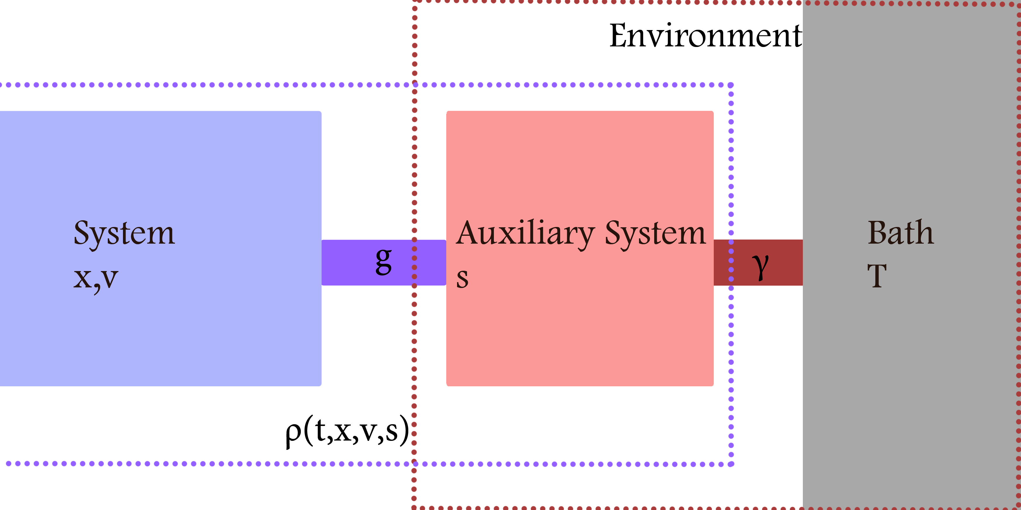
where $g$ is a coupling constant. The situation is illustrated in Fig. 1, for a system with a position coordinate $x$ as well as a velocity. We can solve equation (3) using the integrating factor $\mathrm{e}^{\gamma t}$:

$$s(t)=\int_{-\infty}^{t}\differential t^{\prime}\left(-gv(t^{\prime})+\sqrt{2\gamma T}\xi(t^{\prime})\right)\mathrm{e}^{-\gamma(t-t^{\prime})},$$ (4)

and substitute this into equation (2), giving

$$\begin{split}\derivative{v(t)}{t}=&-g^{2}\int_{-\infty}^{t}\differential t^{\prime}\ v(t^{\prime})\ \mathrm{e}^{-\gamma(t-t^{\prime})}\\ &+g\sqrt{2\gamma T}\int_{-\infty}^{t}\differential t^{\prime}\ \xi(t^{\prime})\ \mathrm{e}^{-\gamma(t-t^{\prime})}.\end{split}$$ (5)

Equation (5) resembles equation (1), except with memory kernels in the friction and noise terms (i.e. it is a generalised Langevin equation). It is a non-Markovian equivalent of the Ornstein-Uhlenbeck process.

The situation is as follows: $v$ is a measurable system parameter (a velocity), and the auxiliary system variable, $s$, is part of the environment, which in this case iscomprised of the auxiliary system and the heat bath which supplies the white noise. We postulate that the variable $s$ has even time-reversal symmetry. The constant $g$ specifies the coupling strength between the particle’s velocity and the environment, and we note that the particle only “sees” the bath indirectly through the auxiliary system. Because $v$ appears in the evolution equation (3) of $s$, the dynamics of the environment are correlated with those of the system. This feature is responsible for the non-Markovian noise and the interesting thermodynamic consequences that this noise causes.

III Interpretation of the Auxiliary System

The degree of freedom $s$ has been designated to be part of the environment, which suggests that it should be considered unmeasurable, much like the huge number of degrees of freedom which make up the heat bath to which it is connected. The utility of baths is that their entropy production can be quantified without needing to measure their microscopic degrees of freedom.

But for a non-Markovian environment this is not true; its correlations with the system mean its behaviour cannot be characterised just by its temperature. This is what makes it more challenging to consider within stochastic thermodynamics, and, of course, all physical environments are to some degree non-Markovian. But we are not obliged to treat the auxiliary system as a physical element of the environment: we can instead simply regard it as a tool that is used in conjunction with the white noise in order to generate a desired memory effect in our system (i.e. equation (5)). By careful use of auxiliary systems, one can imagine the construction of intricate memory kernels while still having a world that, as a whole, is represented by a Markovian bath (or baths) connected to some observable degrees of freedom and thus open to analysis by stochastic thermodynamics.

Some reflection confirms that we are not working at a different level of coarse graining when we introduce an auxiliary system. Varying the level of coarse graining can change the degree of production of entropy in a given process since entropy is dependent on uncertainty, and reduces when we better monitor the evolution of the world. We are merely reformulating the non-Markovian stochastic equations of motion of the system in a fashion that allows standard thermodynamic analysis. The auxiliary system coordinate is a function of system dynamical variables and a noise, as illustrated in equation (4). It is not an unobservable parameter of a physical bath. The entropy production arising from the reformulated dynamics is equivalent to the desired entropy production associated with the non-Markovian stochastic dynamics.

IV The Markovian Limit

The superficial similarities between equations (1) and (5) led us to regard equation (5) as the non-Markovian equivalent of equation (1). We now establish their detailed relationship. We will use the (non-)Markovian case as a shorthand to refer to a system connected to a (non-)Markovian environment.

Setting the coupling constant, $\gamma$, between the auxiliary system and the bath very large allows the integrals in equation (5) to be approximated, but the relationship between the fluctuation and dissipation coefficients in equation (5) doesn’t quite match that in (1). To formulate how the coupling constants should behave in order to maintain this relationship, we consider what must happen to the auxiliary system in order for the environment to be considered Markovian. We assert that in the Markovian limit of our models, $\differential s/\differential t$ must vanish. The best justification for this behaviour is that if $\gamma$ becomes very large, the coupling between the auxiliary system and the bath becomes strong enough that any disturbance in $s$ brought about by the system is immediately dissipated.

However the equivalent Markovian case would not be recovered in the limit $\gamma\rightarrow\infty$ alone, even though this limit offers Markovian dynamics of some sort. The reason for this is as follows. As $\gamma$ increases, the auxiliary system effectively loses its dynamical freedom and never appreciably departs from equilibrium with the bath, no matter the state of the system. However the system is not coupled directly to the bath but just to an auxiliary system that is in a very rigid equilibrium. In a sense the system is attached to a microscopic Markovian bath which consists of one degree of freedom, $s$.

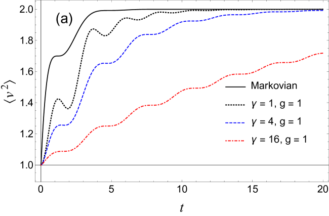
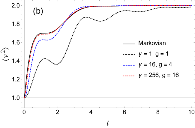
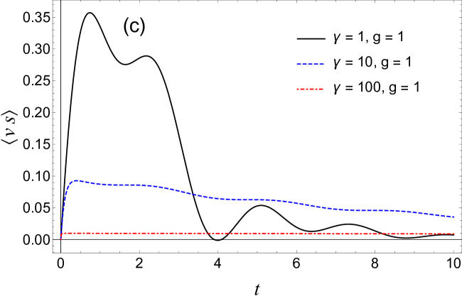
We explore this in Fig. 2 where we study the dynamics of relaxation of the system velocity $v$ in response to an increase of the temperature $T$ of the bath for a variety of coupling strengths $g$ and $\gamma$. A microscopic bath at large $\gamma$ but finite $g$ would not relax the system to equilibrium as quickly as a “genuine” (macroscopic) bath in the absence of an auxiliary system, which is exactly the behaviour seen in Fig. 2 (a). However the dynamics do still become Markovian, as evidenced by the vanishing correlation between $v$ and $s$ in Fig. 2 (c). By increasing the coupling between the system and auxiliary system with the heat bath, $g$, while adopting a large $\gamma$ to preserve the auxiliary system’s equilibrium, we can allow the auxiliary system to transfer enough heat to or from the system to resemble a macroscopic Markovian bath with coupling $\tilde{\gamma}$. The relationship between these parameters turns out to be $g^{2}=\gamma/\tilde{\gamma}$ (see Fig. 2 (b)).

We can motivate this ratio using equation (3). The dissipation from the bath should instantaneously disperse any fluctuations in the auxiliary system coordinate:

$$\derivative{s}{t}=-\gamma s-gv+\sqrt{2\gamma T}\xi\approx 0.$$ (6)

We multiply through by $g/\gamma$ and rearrange:

$$gs=-\frac{g^{2}}{\gamma}v+\sqrt{\frac{2g^{2}T}{\gamma}}\xi,$$ (7)

and substitute into equation (2) to give

$$\derivative{v}{t}=-\tilde{\gamma}v+\sqrt{2\tilde{\gamma}T}\xi,$$ (8)

with $\tilde{\gamma}=g^{2}/\gamma$. A non-Markovian environment can therefore be tuned smoothly to behave like a Markovian bath. We refer to limit of $g,\gamma\rightarrow\infty$ while holding $g^{2}/\gamma$ constant as the Markovian limit of the non-Markovian dynamics We note that since this limit reduces the relaxation time of $s$ to that of the bath, the constants $\gamma$ and $g$ are implicitly a measure of the auxiliary system’s relaxation time.

Figure 2: Evolution of $\langle v^{2}\rangle$ according to equation (5) for an instantaneous change in temperature from $1$ to $2$ at $t=0$, starting at equilibrium, with various auxiliary system-bath coupling strengths with (a): the system-auxiliary system coupling $g$ kept constant, (b): the ratio $g^{2}/\gamma$ maintained at unity; and with the Markovian evolution of $\langle v^{2}\rangle$ according to equation (1) at $\gamma=1$ for reference. (c): Evolution of the system-auxiliary system correlation $\langle vs\rangle$ for a range of auxiliary system-bath coupling strength $\gamma$ with the system-auxiliary system coupling $g$ kept constant. .

V Relaxation of a Tethered Particle

We now consider a tethered harmonic oscillator of unit mass coupled to a non-Markovian environment. The spring constant $\kappa$ is time independent. The Hamiltonian for this system is:

$$\mathscr{H}(x,v)=\frac{1}{2}\kappa x^{2}+\frac{1}{2}v^{2},$$ (9)

where $x$ is the displacement. This allows us to specify the equilibrium statistics of the microscopic variables (irrespective of coupling strengths):

$$\frac{1}{2}\kappa\langle x^{2}\rangle=\frac{1}{2}T,$$ (10)

and similarly for $v$. We postulate that $s$ shares this equilibrium relationship, i.e.

$$\frac{1}{2}\langle s^{2}\rangle=\frac{1}{2}T.$$ (11)

This gives the equilibrium probability density function (pdf) of the system plus auxiliary system a Gaussian form

$$\rho_{{\rm eq}}^{\mathrm{NM}}(x,v,s,T)=\frac{\sqrt{\kappa}}{(2\pi T)^{\frac{3}{2}}}\exp\left(-\frac{\kappa x^{2}}{2T}-\frac{v^{2}}{2T}-\frac{s^{2}}{2T}\right).$$ (12)

We employ the ansatz that the non-equilibrium probability density maintains the Gaussian form, and write:

$$\begin{split}\rho^{\mathrm{NM}}(t,x,v,s)=&\exp\left(N-Ax^{2}-Bv^{2}-Cs^{2}\right.\\ &\left.-Dxv-Exs-Fvs\right).\end{split}$$ (13)

where the coefficients $N$ and $A$ through $F$ are all functions of time $t$.

The stochastic entropy production then has incremental contributions from the system, auxiliary system and the bath seifertreview :

$$\begin{split}\differential\Delta s_{\mathrm{tot}}&=-\differential\ln\rho^{\mathrm{NM}}(t,x,v,s)+\differential\Delta s_{\mathrm{bath}}\\ &=-\differential\ln\rho^{\mathrm{NM}}(t,x,v,s)-\frac{\differential Q}{T},\end{split}$$ (14)

where $\differential Q$ is the incremental heat transferred to the system. We write the equations of motion in Itô form allowing us to use the expression for $\differential\Delta s_{\mathrm{bath}}$ from ref. spinneyfordpre . For simplicity, we set $m=1$ and find

$$\differential x=v\differential t,$$ (15)

$$\differential v=-\kappa x\differential t+gs\differential t,$$ (16)

$$\differential s=-\gamma s\differential t-gv\differential t+\sqrt{2\gamma T}\differential W,$$ (17)

with $\differential W$ an increment of the Wiener process. The total entropy production (see the appendix for derivation) is then

$$\begin{split}\differential\Delta s_{\mathrm{tot}}^{\mathrm{NM}}=&-\differential t\left(2\gamma-4\gamma TC+\gamma TE^{2}x^{2}+\gamma TF^{2}v^{2}+\left(4\gamma TC^{2}-\frac{\gamma}{T}\right)s^{2}+2\gamma TEFxv+4\gamma TCFvs\right)\\ &+\differential W\sqrt{2\gamma T}\left(Ex+Fv+\left(2C-\frac{1}{T}\right)s\right),\end{split}$$ (18)

where $N$ and $A$ to $F$ are found by manipulating the Fokker-Planck equation

$$\begin{split}\partialderivative{\rho^{\mathrm{NM}}}{t}=&-\partialderivative{v\rho^{\mathrm{NM}}}{x}-\partialderivative{(-\kappa x+gs)\rho^{\mathrm{NM}}}{v}-\partialderivative{(-\gamma s-gv)\rho^{\mathrm{NM}}}{s}\\ &+\gamma T\partialderivative[2]{\rho^{\mathrm{NM}}}{s},\end{split}$$ (19)

as shown in the appendix.

Similarly, the pdf for the Markovian dynamics is assumed to take the form

$$\begin{split}\rho^{\mathrm{M}}(t,x,v)=&\exp\left(\tilde{N}-\tilde{A}x^{2}-\tilde{B}v^{2}-\tilde{C}xv\right).\end{split}$$ (20)

The Itô equations of motion in the Markovian case are

$$\differential x=v\differential t,$$ (21)

$$\differential v=-\kappa x\differential t-\tilde{\gamma}v\differential t+\sqrt{2\tilde{\gamma}T}\differential W,$$ (22)

and the increment in total entropy production is

$$\begin{split}\differential\Delta s_{\mathrm{tot}}^{\mathrm{M}}&=-\differential t\left(2\tilde{\gamma}-4\tilde{\gamma}T\tilde{B}+\tilde{\gamma}T\tilde{C}^{2}x^{2}+\left(4\tilde{\gamma}T\tilde{B}^{2}-\frac{\tilde{\gamma}}{T}\right)v^{2}+4\tilde{\gamma}T\tilde{C}xv\right)\\ &+\differential W\sqrt{2\tilde{\gamma}T}\left(\tilde{C}x+\left(2\tilde{B}-\frac{1}{T}\right)v\right),\end{split}$$ (23)

with time dependent functions $\tilde{N}$, $\tilde{A}$, $\tilde{B}$ and $\tilde{C}$ as shown in the appendix.

The total entropy production along a given trajectory for both cases with an isothermal bath is given by integrating equation (14):

$$\Delta s_{\mathrm{tot}}=-\left(\Delta\ln\rho+\frac{Q}{T}\right).$$ (24)

We consider in this case an instantaneous change in the temperature of the environment (i.e. the auxiliary system plus the bath) from $T_{0}$ to $T$. The system in equilibrium at temperature $T_{0}$ is brought into contact with the environment in equilibrium at temperature $T$, for both the Markovian and non-Markovian environments. Because the auxiliary system is part of the environment, the process begins and ends with it in thermal equilibrium at temperature $T$, therefore it contributes nothing to the term $\Delta\ln\rho$ once it has regained equilibrium. The term $Q/T$ therefore determines the difference between the equilibrium to equilibrium entropy productions for the Markovian and non-Markovian cases. The system plus auxiliary system is closed apart from its thermal contact with the bath and therefore the heat transfer exactly equals its energy change. Again, since the auxiliary system starts in thermal equilibrium with the bath, the mean system energy change in the non-Markovian case is the same as that in the Markovian case. Differences inmean entropy production between the Markovian and non-Markovian cases can therefore appear only during non-equilibrium behaviour.

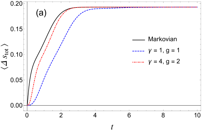
The correlations between the non-Markovian environment and the system mean that the uncertainty in the state of the environment is lower than that of the equivalent Markovian environment; we can salvage some information about it from our knowledge of the system’s evolution. Consequently the mean entropy production in the non-Markovian case will be lower than that of the Markovian case for as long as these non-equilibrium correlations exist. Dynamically speaking, this means the non-Markovian mean entropy production should lag behind the Markovian mean entropy production, reaching the same asymptotic limit but at a later time. Plots of the mean entropy production $\langle\Delta s_{\mathrm{tot}}\rangle$ during the process are shown in Fig. 3 (a). We can quantify this delay by comparing the Markovian mean entropy production, $\langle\Delta s_{\mathrm{tot}}^{\mathrm{M}}\rangle$, with the non-Markovian mean entropy production $\langle\Delta s_{\mathrm{tot}}^{\mathrm{NM}}\rangle$, as follows:

$$\langle\Delta s_{\mathrm{tot}}^{\mathrm{M}}\rangle(t)=\langle\Delta s_{\mathrm{tot}}^{\mathrm{NM}}\rangle(t+\tau(t)).$$ (25)

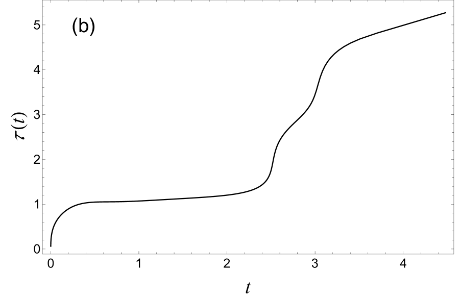
The delay time, $\tau(t)$, illustrated in Fig. 3 (b), describes how much later the non-Markovian case will produce the same amount of entropy, on average, as the Markovian case has produced at time $t$. The utility of this quantity will become clear once we discuss the probability density function (pdf) of the entropy production.

Figure 3: (a): Evolution of $\langle\Delta s_{\mathrm{tot}}\rangle$ (in units such that $k_{\mathrm{B}}=1$) for an instantaneous change in environment temperature from 1 to 2 and various coupling strengths, with the mean entropy production of the Markovian case plotted for reference. (b): The delay time between the Markovian ($\tilde{\gamma}=1$) and non-Markovian ($\gamma=1$, $g=1$) cases that produce a given amount of entropy (see equation (25)).

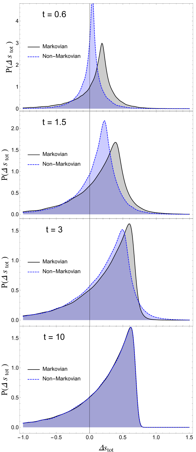
The pdf of entropy production was calculated by simulating 100000 realisations of equations (15) - (17) and constructing histograms of $\Delta s_{\mathrm{tot}}$ as a function of time. This probability density $P(\Delta s_{\mathrm{tot}})$ satisfies a Detailed Fluctuation Theorem fluctuationrelations in the non-Markovian case automatically because the system and auxiliary system combined are attached to a Markovian source of noise. The equilibrium to equilibrium probability density of the entropy production is determined by the change in $\rho$, which is deterministic, and the probability density of the heat transfer (see equation (24)). As discussed, the term $\Delta\ln\rho$ is the same between equilibrium states for both the Markovian and non-Markovian cases. The distribution of heat flow after equilibrium has been reached is also the same because the distributions of the variables $x$ and $v$ in the initial and final equilibrium states are identical. For this reason, the equilibrium to equilibrium probability densities for the entropy production should be identical as well. As can be seen in Fig. 4 this is indeed the case. Notice that the entropy production pdfs have a prominent tail into the negative values. At earlier times, because of the correlations with the auxiliary system (absent in the Markovian case), the pdfs necessarily differ.

Figure 4: Evolution of the pdfs of the entropy production (in units such that $k_{\mathrm{B}}=1$) for an instantaneous change in environment temperature from 1 to 2, for $g=\gamma=1$, with the pdfs of the corresponding entropy production for the Markovian case plotted for reference.

Figure 5: Comparison of the pdfs of the entropy production of the Markovian and non-Markovian cases (from Fig. 4, offset by the delay time shown in Fig. 3 (b).

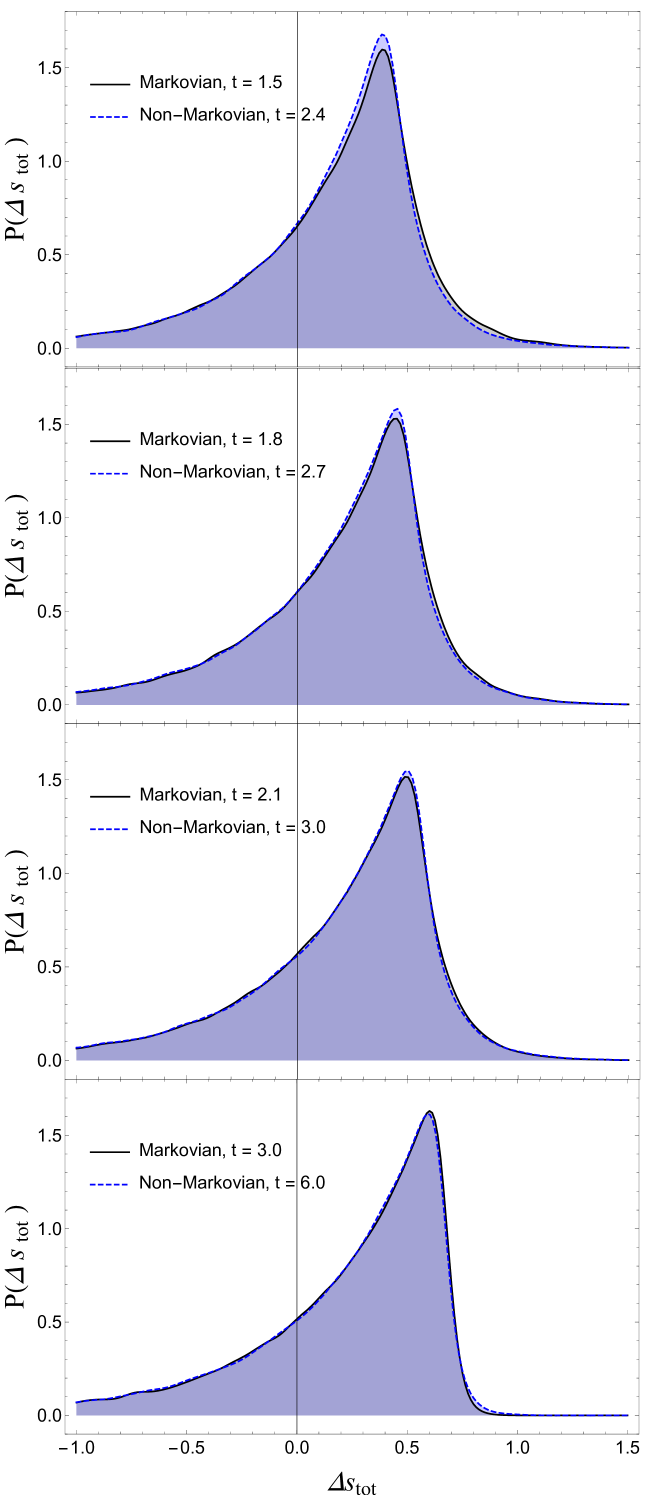
The non-equilibrium pdfs of the dynamical variables of the Markovian and non-Markovian cases are not directly comparable because of the correlation between $s$ and $x$ & $v$. However consideration of Fig. 5 reveals that during relaxation, the pdfs of Markovian and non-Markovian entropy production adopt the same shapes, albeit at different times. The difference between these times is exactly the delay time defined in equation (25) and plotted in Fig. 3 (b). Therefore the Markovian and non-Markovian distributions visit the same sequence of shapes, just at different times.

In summary, the thermodynamics of this type of non-Markovian behaviour suffer a time delay compared to Markovian thermodynamics. We now discuss how non-Markovian environments can affect the thermodynamics when there is a time dependent Hamiltonian.

VI A Dynamically Tethered Particle

The situation we discuss next is a time dependent spring constant $\kappa$ in the tethered system. The Hamiltonian and equations of motion take the same form as before except with time-dependent $\kappa(t)$. The Fokker-Planck equation accommodates $\kappa(t)$ and therefore our generalised Gaussian form for the non-equilibrium pdf of coordinates given by equation (13) remains employable. The work done on the system by changing the spring constant is given by

$$\mathscr{W}=\int_{t_{0}}^{t_{1}}\differential t\ \frac{1}{2}\derivative{\kappa(t)}{t}x(t)^{2}.$$ (26)

We consider a linear change in $\kappa$ between $\kappa_{0}$ and $\kappa_{1}$ over a time period $\Delta t$:

$$\kappa(t)=\begin{cases}\kappa_{0}&t\leq 0\\ \kappa_{0}+(\kappa_{1}-\kappa_{0})\frac{t}{\Delta t}&0\leq t\leq\Delta t\\ \kappa_{1}&t\geq\Delta t\end{cases},$$ (27)

such that the work done becomes

$$\mathscr{W}=\int_{0}^{\Delta t}\differential t\ \frac{1}{2}\frac{(\kappa_{1}-\kappa_{0})}{\Delta t}x(t)^{2}.$$ (28)

In the limiting case $\Delta t\rightarrow 0$ the work done is $\frac{1}{2}(\kappa_{1}-\kappa_{0})x(0)^{2}$ and the Markovian and non-Markovian cases will have identical distributions of work and entropy production for reasons discussed earlier. The asymptotic mean entropy production in this case is fluctuationrelations

$$\langle\Delta s_{\mathrm{tot}}\rangle=\frac{1}{2}\left(\frac{\kappa_{1}}{\kappa_{0}}-1-\ln\left(\frac{\kappa_{1}}{\kappa_{0}}\right)\right).$$ (29)

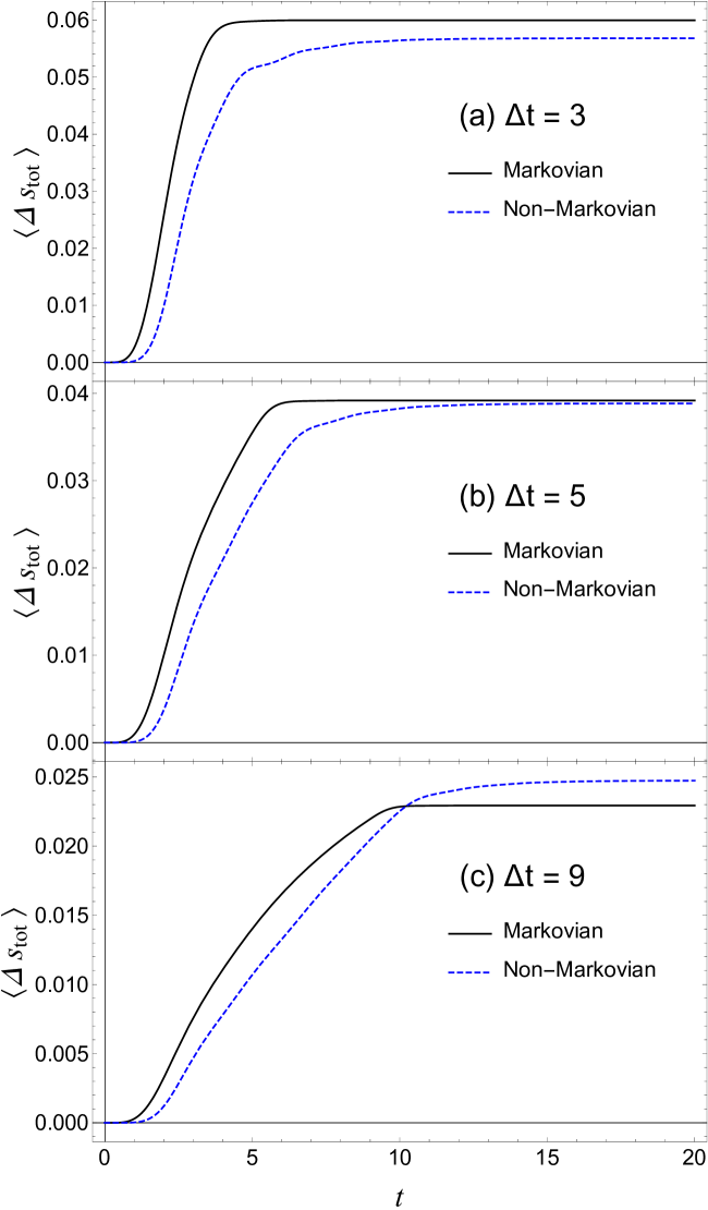
The time evolution of the mean entropy production for this protocol is plotted in Fig. 6. The opposite limit $\Delta t\rightarrow\infty$ is the quasistatic limit. The system and auxiliary system would in this case never depart from equilibrium with the Markovian bath and the entropy production vanishes.

Figure 6: $\langle\Delta s_{\mathrm{tot}}\rangle$ for an instantaneous change in $\kappa$ from 1 to 2 and environmental temperature $T=1$. The non-Markovian case has coupling constants $\gamma=g=1$ and the Markovian case has coupling constant $\tilde{\gamma}=1$. The asymptotic mean entropy production is given by equation (29).

If the spring constant is altered more slowly the mean work done on the system is smaller. The reason for this is as follows: the mean increment in work is given by $\langle\differential\mathscr{W}\rangle=\frac{1}{2}\langle x^{2}\rangle\differential\kappa$. If $\differential\kappa$ is positive the effect of coupling to the environment is for $\langle x^{2}\rangle$ to decrease to match the increased spring constant. Therefore evolving $\kappa$ more slowly will reduce the overall mean work done. The argument for the case when $\differential\kappa$ is negative follows in much the same way. The minimum mean work is therefore performed in the $\Delta t\rightarrow\infty$ limit. Because of this, we expect the non-Markovian case to see more work performed on average than the Markovian case when $\kappa$ is continuously changed since the effects of the bath on the system are delayed (making the integrand in equation (26) larger for longer as a result). A higher mean performance of work implies a greater mean entropy production due to a greater mean transfer of heat into the bath.

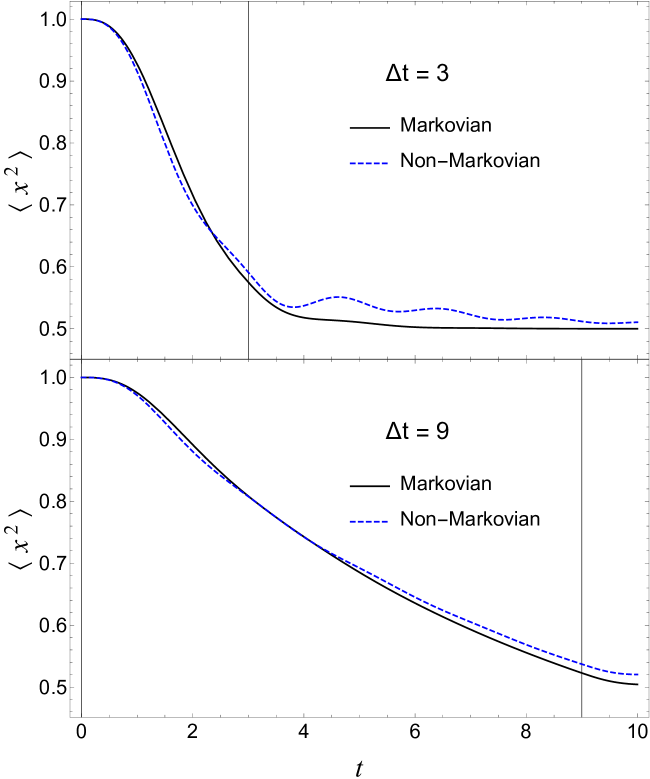
The mean entropy production for Markovian and non-Markovian cases with two protocols of evolution of the spring constant are shown in Fig. 7. Frame (c) is in accord with the prediction just described, but in frame (a) the mean non-Markovian entropy production is lower than that of the Markovian case. Under the logic just proposed this would mean that the variable $x$ evolves more quickly towards equilibrium while the work is being done in the non-Markovian case. Fig. 8 reveals that this is indeed the case: $\langle x^{2}\rangle$ drops more quickly to begin with, though equilibrium is still reached more slowly. A Markovian bath will always behave the same way for a given system - it supplies heat according to its temperature and does not depend on transient correlations with the system - but depending on the nature of the protocol it’s clear that an auxiliary system can either delay or quicken a bath’s influence.

Figure 7: $\langle\Delta s_{\mathrm{tot}}\rangle$ for a uniform rate of change of $\kappa$ from 1 to 2 over different time periods $\Delta t$, with temperature $T=1$. In each case the non-Markovian case has coupling constants $\gamma=g=1$ and the Markovian case has coupling constant $\tilde{\gamma}=1$.

Figure 8: Evolution of $\langle x^{2}\rangle$ for $g=\gamma=1$ in the non-Markovian case and $\tilde{\gamma}=1$ in the Markovian case, $T=1$, and for two different values of $\Delta t$, the duration over which the spring constant $\kappa$ is changed from 1 to 2.

VII A Driven Particle

For our final example we consider an untethered particle subject to a non-conservative oscillatory driving force. With this setup we expect to be able to produce a non-equilibrium oscillatory steady state accompanied by a periodic mean entropy production. The Itô processes defining the dynamics of the non-Markovian case are as follows:

$$\differential v=gs\differential t-\mathscr{F}_{0}\cos(\omega t)\differential t,$$ (30)

$$\differential s=-\gamma s\differential t-gv\differential t+\sqrt{2\gamma T}\differential W.$$ (31)

Here $\mathscr{\mathscr{F}}_{0}$ is a force amplitude, $\omega$ the angular frequency, and the driving force performs work on the system given by

$$\differential\mathscr{W}=-\mathscr{F}_{0}\cos(\omega t)v\differential t.$$ (32)

The Markovian equivalent case has equation of motion:

$$\differential v=-\tilde{\gamma}v\differential t-\mathscr{F}_{0}\cos(\omega t)\differential t+\sqrt{2\tilde{\gamma}T}\differential W.$$ (33)

We assume the following form for the non-Markovian non-equilibrium pdf:

$$\begin{split}\rho^{\mathrm{NM}}(t,v,s)=&\ \mathrm{exp}\left(N(t)-A(t)v^{2}-B(t)vs\right.\\ &\left.-C(t)s^{2}-D(t)v-E(t)s\right),\end{split}$$ (34)

which in contrast to the previous form contains linear terms in the exponent. In the Markovian case we use:

$$\rho^{\mathrm{M}}(t,v)=\mathrm{exp}\left(\tilde{N}(t)-\tilde{A}(t)v^{2}-\tilde{B}(t)v\right).$$ (35)

The increments in total entropy production are:

$$\differential\Delta s_{\mathrm{tot}}^{\mathrm{NM}} =-\differential t\left(2\gamma-4\gamma TC+\gamma TE^{2}+2\gamma TBEv+4\gamma TCEs+\gamma TB^{2}v^{2}+4\gamma TBCvs\right.$$

$$\left.+\left(4\gamma TC^{2}-\frac{\gamma}{T}\right)s^{2}\right)+\differential W\sqrt{2\gamma T}\left(E+Bv+\left(2C-\frac{1}{T}\right)s\right),$$ (36)

and

$$\differential\Delta s_{\mathrm{tot}}^{\mathrm{M}} =-\differential t\left(2\tilde{\gamma}-4\tilde{\gamma}T\tilde{A}+\tilde{\gamma}Tz{\tilde{B}}^{2}+4\tilde{\gamma}T\tilde{A}\tilde{B}v+\left(4\tilde{\gamma}T\tilde{A}^{2}-\frac{\tilde{\gamma}}{T}\right)v^{2}\right)$$

$$+\differential W\sqrt{2\tilde{\gamma}T}\left(\tilde{B}+\left(2\tilde{A}-\frac{v}{T}\right)v\right).$$ (37)

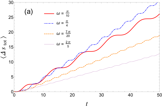
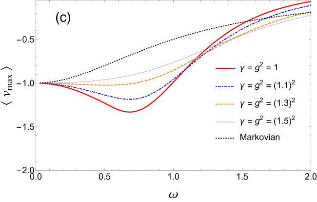
After an initial period a non-equilibrium periodic steady state emerges. Fig. 9 (a) shows that the time derivative of the mean total entropy production goes to zero but never becomes negative, in accordance with the second law of thermodynamics. The mean total entropy production oscillates in the steady state with frequency equal to twice the driving frequency because the dissipative term in equation (31) produces a positive mean entropy production upon both the acceleration and deceleration of $s$. Because this dissipative term $-\gamma s$ (or $-\gamma v$ in the Markovian case) increases as the amplitude $s$ (or $v$) becomes larger in magnitude, increasing the driving frequency without also increasing the force will simply decrease the amplitude and therefore decrease the heat dissipated into the environment.

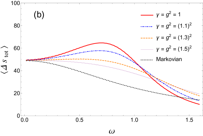
Fig. 9 (b) shows $\langle\Delta s_{\mathrm{tot}}\rangle$ at a given time ($t=100$, which is well within the steady-state regime) as a function of the driving frequency. The Markovian case agrees with the prediction just made. However, in the non-Markovian case the entropy production first increases with frequency before dropping off as expected. As before, this is a consequence of the correlations between the auxiliary system that cause the external protocol (in this case a non-conservative driving force rather than a change of spring constant) to have heightened effects (see the amplitude of oscillation in $\langle v\rangle$ as a function of driving frequency in Fig. 9 (c)).

Figure 9: Evolution of $\langle\Delta s_{\mathrm{tot}}\rangle$ in the periodically driven system (a) as a function of time in the non-Markovian case with $g=\gamma=1$ and $T=1$ for different driving frequencies; (b) as a function of driving frequency at $t=100$ for different coupling constants, $T=1$, and with the Markovian case at $\gamma=1$ for reference. (c) Evolution of $\langle v_{\mathrm{max}}\rangle$, the amplitude of oscillation, as a function of driving frequency at a given time for different coupling constants, with the Markovian case at $\gamma=1$ for reference.

VIII Conclusions

In summary, we have performed an extension of stochastic thermodynamics to environments which can correlate with a system of interest. This was done by interposing an auxiliary system between the system of interest and a heat bath. The system thereby feels the influence of non-Markovian noise while the results of stochastic thermodynamics automatically apply due to the fact that the system plus auxiliary system are still coupled to a Markovian bath.

The presence of memory can heighten or dampen the influence of the environment, depending on the time scales involved. When there is no time-dependent external work protocol and the system merely relaxes, the presence of memory simply serves to delay the equilibration: all distributions of stochastic entropy production lie on the same continuum of distributions exhibited by the equivalent Markovian system. When the external protocol is time-dependent, the combination of non-Markovian thermal coupling and the mechanical coupling can allow the work and entropy production to either exceed or be exceeded by those of the equivalent Markovian system. Because the Markovian approximation is an idealised limit, these observations shed light into how the thermodynamics might differ from this idealisation in systems where time scales aren’t so easily stratified.

The implementation of unphysical degrees of freedom to reproduce the desired memory effects circumvents the difficulty in both the theoretical and computational analysis of memory kernels. The results shown in this work serve as a stimulus for future studies of non-Markovian stochastic thermodynamics using the auxiliary system framework.

Appendix A Solution to Fokker-Planck equations and Derivation of entropy production

The Fokker-Planck equation for the harmonically tethered system coupled to a non-Markovian environment, described in equations (15) - (17), is

$$\begin{split}\partialderivative{\rho^{\mathrm{NM}}}{t}=&-\partialderivative{(v\rho^{\mathrm{NM}})}{x}-\partialderivative{((-\kappa x+gs)\rho^{\mathrm{NM}})}{v}\\ &+\partialderivative{((\gamma s+gv)\rho^{\mathrm{NM}})}{s}+\gamma T\partialderivative[2]{\rho^{\mathrm{NM}}}{t}.\end{split}$$ (38)

Evaluating each of these terms using the trial solution in equation (13) we get:

$$\partialderivative{\rho^{\mathrm{NM}}}{t}=\left(\dot{N}-\dot{A}x^{2}-\dot{B}v^{2}-\dot{C}s^{2}-\dot{D}xv-\dot{E}xs-\dot{F}vs\right)\rho^{\mathrm{NM}},$$ (39)

$$-\partialderivative{(v\rho^{\mathrm{NM}})}{x}=-v(-2Ax-Dv-Es)\rho^{\mathrm{NM}},$$ (40)

$$\partialderivative{(\kappa x\rho^{\mathrm{NM}})}{v}=\kappa x(-2Bv-Dx-Fs)\rho^{\mathrm{NM}},$$ (41)

$$-\partialderivative{(gs\rho^{\mathrm{NM}})}{v}=-gs(-2Bv-Dx-Fs)\rho^{\mathrm{NM}},$$ (42)

$$\partialderivative{(\gamma s\rho^{\mathrm{NM}})}{s}=\gamma\rho^{\mathrm{NM}}+\gamma s(-2Cs-Ex-Fv)\rho^{\mathrm{NM}},$$ (43)

$$\partialderivative{(gv\rho^{\mathrm{NM}})}{s}=gv(-2Cs-Ex-Fv)\rho^{\mathrm{NM}},$$ (44)

$$\gamma T\partialderivative[2]{\rho^{\mathrm{NM}}}{s}=\gamma T(-2Cs-Ex-Fv)^{2}\rho^{\mathrm{NM}}+\gamma T(-2C)\rho^{\mathrm{NM}}.$$ (45)

From here we can read off the coefficients to $\rho^{\mathrm{NM}}$, $x^{2}\rho^{\mathrm{NM}}$, $xv\rho^{\mathrm{NM}}$ etc to write down the evolution equations for $N$ and $A-F$:

$$\dot{N}=\gamma-2\gamma TC,$$ (46)

$$-\dot{A}=-\kappa D+\gamma TE^{2},$$ (47)

$$-\dot{B}=D-gF+\gamma TF^{2},$$ (48)

$$-\dot{C}=gF-2\gamma C+4\gamma TC^{2},$$ (49)

$$-\dot{D}=2A-2\kappa B-gE+2\gamma TEF,$$ (50)

$$-\dot{E}=-\kappa F+gD-\gamma E+4\gamma TCE,$$ (51)

$$-\dot{F}=E+2gB-gE-\gamma F-2gC+4\gamma TCF.$$ (52)

The total entropy production is written $\differential\Delta s_{\mathrm{tot}}^{{\rm{NM}}}=\differential\Delta s_{\mathrm{sys}}^{{\rm{NM}}}+\differential\Delta s_{\mathrm{bath}}^{{\rm{NM}}}$. We compute the first contribution from the pdf over dynamical variables:

$$\begin{split}\differential\Delta s_{\mathrm{sys}}^{{\rm{NM}}}&=-\differential\ln\rho^{\mathrm{NM}}\\ &=-\partialderivative{\ln\rho^{\mathrm{NM}}}{t}\differential t-\partialderivative{\ln\rho^{\mathrm{NM}}}{x}\differential x-\partialderivative{\ln\rho^{\mathrm{NM}}}{v}\differential v\\ &-\partialderivative{\ln\rho^{\mathrm{NM}}}{s}\differential s-\gamma T\partialderivative[2]{\ln\rho^{\mathrm{NM}}}{s}\differential t,\end{split}$$ (53)

where we’ve used Itô’s lemma. Again, we compute each term:

$$-\partialderivative{\ln\rho^{\mathrm{NM}}}{t}\differential t=-\dot{N}+\dot{A}x^{2}+\dot{B}v^{2}+\dot{C}s^{2}+\dot{D}xv+\dot{E}xs+\dot{F}vs,$$ (54)

$$-\partialderivative{\ln\rho^{\mathrm{NM}}}{x}\differential x=(2Ax+Dv+Es)(v\differential t),$$ (55)

$$-\partialderivative{\ln\rho^{\mathrm{NM}}}{v}\differential v=(2Bv+Dx+Fs)(-\kappa x\differential t++gs\differential t),$$ (56)

$$-\partialderivative{\ln\rho^{\mathrm{NM}}}{s}\differential s=(2Cs+Ex+Fs)(-\gamma s\differential t-gv\differential t+\sqrt{2\gamma T}\differential W),$$ (57)

$$-\gamma T\partialderivative[2]{\ln\rho^{\mathrm{NM}}}{s}=2\gamma TC\differential t.$$ (58)

The entropy production in the bath is given by $\differential Q/T$, where $Q$ is the heat flow into the bath from the auxiliary system. The energy of the auxiliary system can change either by this heat flow or by doing work on the system. To identify these components, we examine the energy differential of the auxiliary system (using Itô’s lemma):

$$\begin{split}\frac{1}{2}\differential\left(s^{2}\right)=&\frac{1}{2}\left(2s\differential s+2\gamma T\differential t\right)\\ =&\frac{1}{2}\Big{(}-2\gamma s^{2}\differential t-2gvs\differential t+2s\sqrt{2\gamma T}\differential W\\ &+2\gamma T\differential t\Big{)}\\ =&\left(-\gamma s^{2}-gvs+\gamma T\right)\differential t+s\sqrt{2\gamma T}\differential W.\end{split}$$ (59)

By inspection of the system’s kinetic energy, we can identify the $gvs\differential t$ as the differential of the work done by the coupling between the system and auxiliary system:

$$\begin{split}\frac{1}{2}\differential\left(v^{2}\right)=&2v\differential v\\ =&-\kappa xv\differential t+gvs\differential t.\end{split}$$ (60)

The remaining part of Eq. 59 is therefore the heat flow to the bath, which allows us to identify the entropy production in the bath:

$$\begin{split}\differential\Delta s_{\mathrm{bath}}^{{\rm{NM}}}&=-\frac{\differential Q}{T},\\ &=-\frac{\differential(s^{2})}{T}-\frac{1}{T}gvs\differential t,\\ &=\differential t\left(\frac{\gamma s^{2}}{T}-\gamma\right)+\differential W\left(\frac{s}{T}\sqrt{2\gamma T}\right),\end{split}$$ (61)

again using Itô’s lemma. The same expression can be derived using considerations laid out in spinneyfordpre . Then we substitute equations (54 - 58) into equation (53), add that to (61), and then compare coefficients of terms in $\differential W$, $\differential t$, $x^{2}\differential t$, $xv\differential t$ etc. Most of the terms in equations (46 - 52) cancel, and the final result is equation (18).

The Fokker-Planck equation for the Markovian dynamical system described in equations (21) - (22) is

$$\begin{split}\partialderivative{\rho^{\mathrm{M}}}{t}=&-\partialderivative{(v\rho^{\mathrm{M}})}{x}-\partialderivative{((-\kappa x-\tilde{\gamma}v)\rho^{\mathrm{M}})}{v}\\ &+\tilde{\gamma}T\partialderivative[2]{\rho^{\mathrm{M}}}{t},\end{split}$$ (62)

and as for the non-Markovian case we write:

$$\partialderivative{\rho^{\mathrm{M}}}{t}=\left(\dot{\tilde{N}}-\dot{\tilde{A}}x^{2}-\dot{\tilde{B}}v^{2}-\dot{\tilde{C}}xv\right)\rho^{\mathrm{M}}$$ (63)

$$-\partialderivative{(v\rho^{\mathrm{M}})}{x}=-v(-2\tilde{A}x-\tilde{C}v)\rho^{\mathrm{M}},$$ (64)

$$\partialderivative{(\kappa x\rho^{\mathrm{M}})}{v}=\kappa x(-2\tilde{B}v-\tilde{C}x)\rho^{\mathrm{M}},$$ (65)

$$\partialderivative{(\tilde{\gamma}v\rho^{\mathrm{M}})}{v}=\tilde{\gamma}\rho^{\mathrm{M}}+\tilde{\gamma}v(-2\tilde{B}v-\tilde{C}x)\rho^{\mathrm{M}},$$ (66)

$$\tilde{\gamma}T\partialderivative[2]{\rho^{\mathrm{M}}}{v}=\tilde{\gamma}T(-2\tilde{B}v-\tilde{C}x)^{2}\rho^{\mathrm{M}}+\tilde{\gamma}T(-2\tilde{B})\rho^{\mathrm{M}}.$$ (67)

Again we read off the coefficients to write down the evolution equations:

$$\dot{\tilde{N}}=\tilde{\gamma}-2\tilde{\gamma}T\tilde{B},$$ (68)

$$-\dot{\tilde{A}}=-\kappa\tilde{C}+\tilde{\gamma}T\tilde{C}^{2},$$ (69)

$$-\dot{\tilde{B}}=\tilde{C}-2\tilde{\gamma}\tilde{B}+4\tilde{\gamma}T\tilde{B}^{2},$$ (70)

$$-\dot{\tilde{C}}=2\tilde{A}-2\kappa\tilde{B}-\tilde{\gamma}\tilde{C}+4\tilde{\gamma}T\tilde{B}\tilde{C}.$$ (71)

We substitute these into the system entropy production:

$$\begin{split}\differential\Delta s_{\mathrm{sys}}^{{\rm{M}}}&=-\differential\ln\rho^{\mathrm{M}}\\ &=-\partialderivative{\ln\rho^{\mathrm{M}}}{t}\differential t-\partialderivative{\ln\rho^{\mathrm{M}}}{x}\differential x-\partialderivative{\ln\rho^{\mathrm{M}}}{v}\differential v\\ &-\tilde{\gamma}T\partialderivative[2]{\ln\rho^{\mathrm{M}}}{v}\differential t,\end{split}$$ (72)

where we’ve used Itô’s lemma. Again, we decompose each term.

$$-\partialderivative{\ln\rho^{\mathrm{M}}}{t}\differential t=-\dot{\tilde{N}}+\dot{\tilde{A}}x^{2}+\dot{\tilde{B}}v^{2}+\dot{\tilde{C}}xv,$$ (73)

$$-\partialderivative{\ln\rho^{\mathrm{M}}}{x}\differential x=(2\tilde{A}x+\tilde{C}v)(v\differential t),$$ (74)

$$-\partialderivative{\ln\rho^{\mathrm{M}}}{v}\differential v=(2\tilde{B}v+\tilde{C}x)(-\kappa x\differential t-\tilde{\gamma}v\differential t+\sqrt{2\tilde{\gamma}T}\differential W),$$ (75)

$$-\tilde{\gamma}T\partialderivative[2]{\ln\rho^{\mathrm{M}}}{s}=2\tilde{\gamma}TC\differential t.$$ (76)

The bath term is

$$\begin{split}\differential\Delta s_{\mathrm{bath}}^{{\rm{M}}}&=-\frac{\differential Q}{T},\\ &=-\frac{\differential(v^{2})}{T}-\kappa xv\frac{1}{T}\differential t,\\ &=-\frac{2v\differential v}{T}-\tilde{\gamma}\differential t,\\ &=\differential t\left(\frac{\tilde{\gamma}v^{2}}{T}-\tilde{\gamma}\right)+\differential W\left(\frac{v}{T}\sqrt{2\tilde{\gamma}T}\right).\end{split}$$ (77)

Proceeding in the same way as the non-Markovian case, substitution and cancellation results in equation (23).

Similar procedures are followed to solve the appropriate Fokker-Planck equations and derive entropy productions in the other example cases.

References

- (1) D. J. Evans, E. G. D. Cohen, and G. P. Morriss, Phys. Rev. Lett. 71, 2401 (1993).
- (2) D. J. Evans and D. J. Searles, Phys. Rev. E 52, 5839 (1995).
- (3) D. J. Evans, and D. J. Searles, Adv. Phys. 51, 1529 (2002).
- (4) D. M. Carberry, J. C. Reid, G. M. Wang, E. M. Sevick, D. J. Searles, and D. J Evans, Phys. Rev. Lett. 92, 140601 (2004).
- (5) U. Seifert, Rep. Prog. Phys. 75, 12 (2012).
- (6) K. Sekimoto, Prog. Theor. Phys. Suppl. 130, 17 (1998).
- (7) R. Zwanzig, Nonequilibrium Statistical Mechanics, Oxford University Press (2001).
- (8) L. Stella, C. D. Lorenz, and L. Kantorovich, Phys. Rev. B 89, 134303 (2014).
- (9) M. Ceriotti, G. Bussi, and M. Parrinello, Phys. Rev. Lett. 102, 020601 (2009).
- (10) L. Kantorovich, Phys. Rev. B 78, 094304 (2008).
- (11) J. A. Morrone, T. E. Markland, M. Ceriotti, and B. J. Berne, J. Chem. Phys. 134, 014103 (2011).
- (12) A. Kutvonen, T. Ala-Nissila, and J. Pekola, Phys. Rev. E 92. 012107 (2015).
- (13) P. Strasberg, G. Schaller, N. Lambert, and T. Brandes, New J. Phys. 18, 073007 (2016).
- (14) A. Kato, and Y. Tanimura, J. Chem. Phys. 145, 224105 (2016).
- (15) C. Wang, J. Ren, J. Cao, Sci. Rep. 5, 11787 (2015).
- (16) L. Nicolin and D. Segal, Phys. Rev. B 84, 161414(R) (2011).
- (17) A. Fulinski, Z. Grzywana, I. Mellor, Z. Siwy, and P. N. R. Usherwood, Phys. Rev. E 58, 919 (1998).
- (18) A. Garg, J. N. Onuchic, and V. Ambegaokar, J. Chem. Phys. 83, 4491 (1985).
- (19) T. Speck and U. Seifert, J. Stat. Mech. L009002 (2007).
- (20) U. Seifert, Phys. Rev. Lett. 116, 020601 (2016).
- (21) M. Campisi, P. Talkner, and P. HÀnggi, Phys. Rev. Lett. 102, 210401 (2009).
- (22) C. Jarzynski, J. Stat. Mech. P09005 (2004).
- (23) T. Kawamoto and N. Hanato, Phys. Rev. E 87, 032113 (2013).
- (24) T. Ohkuma and T. Ohta, J. Stat. Mech. 10, P10010 (2007).
- (25) H. Miller and J. Anders, Phys. Rev. E 95,062123 (2017).
- (26) R. Martinazzo, K. H. Hughes, and I. Burghardt, Phys. Rev. E 84, 030102 (2011).
- (27) M. P. Woods, R. Groux, A. W. Chin, S. F. Huelga, and M. B. Plenio, J. Math. Phys. 55, 032101 (2014).
- (28) A. W. Chin, A. Rivas, S. F. Huelga, M. B. Plenio, J. Math. Phys. 51, 092109 (2010).
- (29) R. E. Spinney and I. J. Ford, Phys. Rev. E 85 051113 (2012).
- (30) R. E. Spinney and I. J. Ford, Fluctuation Relations: A Pedagogical Overview, in Klages, R., Just, W., Jarzynski, C. ed. Nonequilibrium Statistical Physics of Small Systems: Fluctuation Relations and Beyond, Wiley-VCH, Weinheim, ISBN 978-3-527-41094-1, (2013).